NBER WORKING PAPER SERIES

MEASURING THE UNEQUAL GAINS FROM TRADE

Pablo D. FajgelbaumAmit K. Khandelwal

Working Paper 20331http://www.nber.org/papers/w20331

NATIONAL BUREAU OF ECONOMIC RESEARCH1050 Massachusetts Avenue

Cambridge, MA 02138July 2014

We thank Andrew Atkeson, Joaquin Blaum, Ariel Burstein, Arnaud Costinot, Robert Feenstra, JuanCarlos Hallak, Esteban Rossi-Hansberg, Nina Pavcnik, Jonathan Vogel and seminar participants atBrown, Chicago, Cowles, ERWIT, Harvard, NBER ITI, Princeton, Stanford, UCLA, USC, and theInternational Growth Centre meeting at Berkeley for helpful comments. We acknowledge fundingfrom the Jerome A. Chazen Institute of International Business at Columbia Business School. The viewsexpressed herein are those of the authors and do not necessarily reflect the views of the National Bureauof Economic Research.

NBER working papers are circulated for discussion and comment purposes. They have not been peer-reviewed or been subject to the review by the NBER Board of Directors that accompanies officialNBER publications.

© 2014 by Pablo D. Fajgelbaum and Amit K. Khandelwal. All rights reserved. Short sections of text,not to exceed two paragraphs, may be quoted without explicit permission provided that full credit,including © notice, is given to the source.

Measuring the Unequal Gains from TradePablo D. Fajgelbaum and Amit K. KhandelwalNBER Working Paper No. 20331July 2014, Revised August 2015JEL No. D63,F10,F60

ABSTRACT

Individuals that consume different baskets of goods are differentially affected by relative price changescaused by international trade. We develop a methodology to measure the unequal gains from tradeacross consumers within countries. The approach requires data on aggregate expenditures and parametersestimated from a non-homothetic gravity equation. We find that trade typically favors the poor, whoconcentrate spending in more traded sectors.

Pablo D. FajgelbaumDepartment of EconomicsUniversity of California, Los Angeles8283 Bunche HallLos Angeles, CA 90095and NBERpfajgelbaum@gmail.com

Amit K. KhandelwalGraduate School of BusinessColumbia UniversityUris Hall 606, 3022 BroadwayNew York, NY 10027and NBERak2796@columbia.edu

1 Introduction

Understanding the distributional impact of international trade is one of the central tasks pursued

by international economists. A vast body of research has examined this question through the effect

of trade on the distribution of earnings across workers (e.g., Stolper and Samuelson 1941). A second

channel operates through the cost of living. It is well known that the consumption baskets of high-

and low-income consumers look very different (e.g., Deaton and Muellbauer 1980b). International

trade therefore has a distributional impact whenever it affects the relative price of goods that are

consumed at different intensities by rich and poor consumers. For example, a trade-induced increase

in the price of food has a stronger negative effect on low-income consumers, who typically have

larger food expenditure shares than richer consumers. How important are the distributional effects

of international trade through this expenditure channel? How do they vary across countries? Do

they typically favor high- or low- income consumers?

In this paper we develop a methodology to answer these questions. The approach is based on

aggregate statistics and model parameters that can be estimated from readily available bilateral

trade and production data. It can therefore be implemented across many countries and over time.

A recent literature in international trade, including Arkolakis et al. (2012), Melitz and Redding

(2014) and Feenstra and Weinstein (2010), measures the aggregate welfare gains from trade by

first estimating model parameters from a gravity equation (typically, the elasticity of imports with

respect to trade costs) and then combining these parameters with aggregate statistics to calculate

the impact of trade on aggregate real income. We estimate model parameters from a non-homothetic

gravity equation (the elasticity of imports with respect to both trade costs and income) to calculate

the impact of trade on the real income of consumers with different expenditures within the economy.

The premise of our analysis is that consumers at different income levels within an economy may

have different expenditure shares in goods from different origins or in different sectors. Studying

the distributional implications of trade in this context requires a non-homothetic demand structure

with good-specific Engel curves, where the elasticity of the expenditure share with respect to

individuals’ total expenditures is allowed to vary across goods. The Almost-Ideal Demand System

(AIDS) is a natural choice. As first pointed out by Deaton and Muellbauer (1980a), it is a first-

order approximation to any demand system; importantly for our purposes, it is flexible enough

to satisfy the key requirement of good-specific income elasticities and has convenient aggregation

properties that allow us to accommodate within-country inequality.

We start with a demand-side result: in the AIDS, the welfare change through the expenditure

channel experienced by consumers at each expenditure level as a result of changes in prices, can

be recovered from demand parameters and aggregate statistics. These aggregate statistics include

the initial levels and changes in aggregate expenditure shares across commodities, and moments

from the distribution of expenditure levels across consumers. The intuition for this result is that,

conditioning on moments of the expenditure distribution, changes in aggregate expenditure shares

across goods can be mapped to changes in the relative prices of high- versus low-income elastic

goods by inverting the aggregate demand. These relative price changes and demand parameters, in

1

turn, suffice to measure the variation in real income of consumers at each expenditure level through

changes in the cost of living.

To study the distributional effects of trade through the expenditure channel we embed this

demand structure into a standard model of international trade, the multi-sector Armington model.

This simple supply side allows us to cleanly highlight the methodological innovation on the demand

side.1 The model allows for cross-country differences in sectoral productivity and bilateral trade

costs, and within each sector goods are differentiated by country of origin. We extend this supply-

side structure with two features. First, the endowment of the single factor of production varies

across consumers, generating within-country inequality. Second, consumer preferences are given

by the AIDS, allowing goods from each sector and country of origin to enter with different income

elasticity into the demand of individual consumers. As a result, aggregate trade patterns are driven

both by standard Ricardian forces (differences in productivities and trade costs across countries

and sectors) and by demand forces (cross-country differences in income distribution and differences

in the income elasticity of exports by sector and country).

In the model, differences between the income elasticities of exported and imported goods shape

the gains from trade-cost reductions of poor relative to rich consumers within each country. We

show how to use demand-side parameters and changes in aggregate expenditure shares to measure

welfare changes experienced by consumers at different income levels in response to foreign shocks.

For example, a tilt in the aggregate import basket towards goods consumed mostly by the rich may

reveal a fall in the import prices of these goods, and a relative welfare improvement for high-income

consumers. In countries where exports are high-income elastic relative to imports, the gains from

trade are relatively biased to poorer consumers because opening to trade decreases the relative

price of low-income elastic goods. Non-homotheticity across sectors also shape the unequal gains

from trade across consumers because sectors vary in their tradeability (e.g., food versus services)

and in the substitutability across goods supplied by different exporters.

To quantify the unequal gains from trade, we need estimates of the elasticity of individual

expenditure shares by sector and country of origin with respect to both prices and income. A

salient feature of the model is that it delivers a sectoral non-homothetic gravity equation to estimate

these key parameters from readily-available data on production and trade flows. The estimation

identifies which countries produce high or low income-elastic goods by projecting budget shares

within each sector on standard gravity forces (e.g., distance, border and common language) and a

summary statistic of the importer’s income distribution whose elasticity can vary across exporters.2

Consistent with the existing empirical literature, such as Hallak and Schott (2011) and Feenstra

and Romalis (2014), we find that richer countries export goods with higher income elasticities

within sectors. The estimation also identifies the sectors whose goods are relatively more valued by

1For example, the model abstracts away from forces that would lead to distributional effects through changes inthe earnings distribution, as well as differentiated exporters within sectors, firm heterogeneity, competitive effects, orinput-output linkages. Future work could consider embedding the AIDS into models with a richer supply side.

2When non-homotheticities are shut down, the gravity equation in our model corresponds to the translog gravityequation estimated by Novy (2012) and Feenstra and Weinstein (2010).

2

rich consumers by projecting sectoral expenditure shares on a summary statistic of the importer’s

income distribution. Consistent with Hallak (2010), our results also suggest non-homotheticities

not only across origin countries but also across sectors.

Using the estimated parameters, we apply the results from the theory to ask: who are the

winners and losers of trade within countries, how large are the distributional effects, and what

country characteristics are important to shape these effects? To answer these questions we perform

the counterfactual exercise of increasing trade costs so that each country is brought from its current

trade shares to autarky, and compute the gains from trade corresponding to each percentile of the

income distribution in each country (i.e., the real income that would be lost by each percentile

because of a shut down of trade).

We find a pro-poor bias of trade in every country. On average, the real income loss from closing

off trade is 63 percent at the 10th percentile of the income distribution and 28 percent for the

90th percentile. This bias in the gains from trade toward poor consumers hinges on the fact that

these consumers spend relatively more on sectors that are more traded, while high-income indi-

viduals consume relatively more services, which are among the least traded sectors. Additionally,

low-income consumers happen to concentrate spending on sectors with a lower elasticity of sub-

stitution across source countries. Larger expenditures in more tradeable sectors and a lower rate

of substitution between imports and domestic goods lead to larger gains from trade for the poor

than the rich. While this pro-poor bias of trade is present in every country, there is heterogeneity

in the difference between the gains from trade of poor and rich consumers across countries. In

countries with a lower income elasticity of exports, the gains from trade tend to be less favorable

for poor consumers because opening to trade causes an increase in the relative price of low-income

elastic goods. Similar results appear in counterfactuals involving smaller changes in trade costs

than a movement to autarky; for example, a small reduction in the cost of importing in the food or

manufacturing sectors also exhibits a pro-poor bias. However, trade-cost reductions affecting only

the service sectors (which are relatively high-income elastic) benefits the rich relatively more.

As we mentioned, our approach to measure welfare gains from trade using aggregate statistics

is close to a recent literature that studies the aggregate welfare gains from trade summarized by

Costinot and Rodriguez-Clare (2014). This literature confronts the challenge that price changes

induced by trade costs are not commonly available by inferring them through the model structure

from changes in trade shares.3 These approaches are designed to measure only aggregate gains

rather than distributional consequences.4 In our setting, we exploit properties of a non-homothetic

demand system that also allows us to infer changes in prices from trade shares and to trace out the

welfare consequences of these price changes across different consumers within countries. We are

motivated by the belief that an approach that is able to quantify the (potentially) unequal gains

3For example, autarky prices are rarely observed in data but under standard assumptions on preferences theautarky expenditure shares are generally known. The difference between autarky and observed trade shares can thenbe used to back out the price changes caused by a counterfactual movement to autarky.

4Two exceptions are Burstein and Vogel (2012) and Galle et al. (2014), which use aggregate trade data to estimatethe effects of trade on the distribution of earnings.

3

from trade through the expenditure channel for many countries is useful in assessing the implications

of trade, particularly because much of the public opposition towards increased openness stems from

the belief that welfare changes are unevenly distributed.

Of course, we are not the first to allow for differences in income elasticities across goods in

an international trade framework. Theoretical contributions to this literature including Markusen

(1986), Flam and Helpman (1987) and Matsuyama (2000) develop models where richer countries

specialize in high-income elastic goods through supply-side forces, while Fajgelbaum et al. (2011)

study cross-country patterns of specialization that result from home market effects in vertically

differentiated products. Recent papers by Hallak (2006), Fieler (2011), Caron et al. (2014) and

Feenstra and Romalis (2014) find that richer countries export goods with higher income elasticity.5

This role of non-homothetic demand and cross-country differences in the income elasticity of exports

in explaining trade data is an important motivation for our focus on explaining the unequal gains

from trade through the expenditure channel.

These theoretical and empirical studies use a variety of demand structures. To our knowledge,

only a few studies have used the AIDS in the international trade literature: Feenstra and Reinsdorf

(2000) show how prices and aggregate expenditures relate to the Divisia index in the AIDS and

suggest that this demand system could be useful for welfare evaluation in a trade context, Feenstra

(2010) works with a symmetric AIDS expenditure function to study the entry of new goods, and

Chaudhuri et al. (2006) use the AIDS to determine the welfare consequences in India of enforcing

the Agreement on Trade-Related Intellectual Property Rights.6 Neary (2004) and Feenstra et al.

(2009) use the AIDS for making aggregate real income comparisons across countries and over time

using data from the International Comparison Project. Aguiar and Bils (2015) estimated an AIDS

in the U.S. to measure inequality in total consumption expenditures from consumption patterns.

A few papers study the effect of trade on inequality through the expenditure channel. Porto

(2006) studies the effect of price changes implied by a tariff reform on the distribution of welfare

using consumer survey data from Argentina, Faber (2013) exploits Mexico’s entry into NAFTA to

study the effect of input tariff reductions on the price changes of final goods of different quality,

and Atkin et al. (2015) studies the effect of foreign retailers on consumer prices in Mexico. While

these papers utilize detailed microdata for specific countries in the context of major reforms, our

approach provides a framework to quantify the unequal gains from trade across consumers over a

large set of countries using aggregate trade and production data. Within our framework we are able

to show theoretically how changes in trade costs map to the welfare changes of individuals in each

point of the expenditure distribution, how to compute these effects using model parameters and

aggregate statistics, and how to estimate the parameters from cross-country trade and production

5See also Schott (2004), Hallak and Schott (2011) and Khandelwal (2010) who provide evidence that richercountries export higher-quality goods, which typically have high income elasticity of demand. In this paper weabstract from quality differentiation within sectors, but note that our methodology could be implemented usingdisaggregated trade data where differences in the income elasticity of demand may be driven by differences in quality.

6If good-specific income elasticities are neutralized, the AIDS collapses to the homothetic translog demand systemstudied in an international trade context by Kee et al. (2008), Feenstra and Weinstein (2010), Arkolakis et al. (2010)and Novy (2012).

4

data.

There is of course a large literature that examines trade and inequality through the earnings

channel. A dominant theme in this literature, as summarized by Goldberg and Pavcnik (2007),

has been the poor performance of Stolper-Samuelson effects, which predict that trade increases

the relative wages of low-skill workers in countries where these workers are relatively abundant, in

rationalizing patterns from low-income countries.7 We complement these and other studies that

focus on the earnings channel by examining the implications of trade through the expenditure

channel.

The remainder of the paper is divided into five sections. Section 2 uses standard consumer

theory to derive generic expressions for the distribution of welfare changes across consumers, and

applies these results to the AIDS. Section 3 embeds these results in a standard trade framework,

derives the non-homothetic gravity equation, and provides the expressions to determine the gains

from trade across consumers. Section 4 estimates the key elasticities from the gravity equation.

Section 5 presents the results of counterfactuals that simulate foreign-trade cost shocks. Section 6

concludes.

2 Consumers

We start by deriving generic expressions for the distribution of welfare changes in response to

price changes across consumers that vary in their total expenditures. We only use properties of

demand implied by standard demand theory. In Section 3, we link these results to a standard

model of trade in general equilibrium.

2.1 Definition of the Expenditure Channel

We study an economy with J goods for final consumption with price vector p = pjJj=1 taken

as given by h = 1, ..,H consumers. Consumer h has indirect utility vh and total expenditures xh.

We denote the indirect utility function by v (xh,p). We let sj,h ≡ sj (xh,p) be the share of good

j in the total expenditures of individual h, and Sj =∑

h

(xh∑h′ xh′

)sj,h be the share of good j in

aggregate expenditures.

Consider the change in the log of indirect utility of consumer h due to infinitesimal changes in

log-prices pjJj=1 and in the log of the expenditure level xh:8

vh =

J∑j=1

∂ ln v (xh,p)

∂ ln pjpj +

∂ ln v (xh,p)

∂ lnxhxh. (1)

The equivalent variation of consumer h associated with pjJj=1 and xh is defined as the change in

7Several recent studies, such as Feenstra and Hanson (1996), Helpman et al. (2012), Brambilla et al. (2012),Frias et al. (2012), and Burstein et al. (2013) study different channels through which trade affects the distribution ofearnings such as outsourcing, labor market frictions, quality upgrading, or capital-skill complementarity.

8Throughout the paper we use z ≡ d ln (z) to denote the infinitesimal change in the log of variable z.

5

log expenditures, ωh, that leads to the indirect utility change vh at constant prices:

vh =∂ ln v (xh,p)

∂ lnxhωh. (2)

Combining (1) and (2) and applying Roy’s identity gives a well-known formula for the equivalent

variation:9

ωh =

J∑j=1

(−pj) sj,h + xh. (3)

The first term on the right-hand side of (3) is an expenditure-share weighted average of price

changes. It represents what we refer to as the expenditure effect. It is the increase in the cost of

living caused by a change in prices applied to the the pre-shock expenditure basket. Henceforth, we

refer to ωh as the welfare change of individual h, acknowledging that by this we mean the equivalent

variation, expressed as share of the initial level of expenditures, associated with a change in prices

or in the expenditure level of individual h.

To organize our discussion it is useful to rewrite (3) as follows:

ωh = W + ψh + xh, (4)

where

W ≡J∑j=1

(−pj)Sj , (5)

is the aggregate expenditure effect, and

ψh ≡J∑j=1

(−pj) (sj,h − Sj) (6)

is the individual expenditure effect of consumer h.

The term W is the welfare change through the expenditure channel that corresponds to every

consumer either in the absence of within-country inequality or under homothetic preferences. It also

corresponds to the welfare change through the cost of expenditures for a hypothetical representative

consumer. In turn, the term ψh captures that consumers may be differentially affected by the same

price changes due to differences in the composition of their expenditure basket. It is different

from zero for some consumers only if there is variation across consumers in how they allocate

expenditure shares across goods. The focus of this paper is to study how international trade

impacts the distributionψh

Hh=1

.

9See Theil (1975).

6

2.2 Almost-Ideal Demand

The Almost-Ideal Demand System (AIDS) introduced by Deaton and Muellbauer (1980a) be-

longs to the family of Log Price-Independent Generalized Preferences defined by Muellbauer (1975).

The latter are defined by the indirect utility function

v (xh,p) = F

[(xha (p)

)1/b(p)], (7)

where a (p) and b (p) are price aggregators and F [·] is a well-behaved increasing function. The

AIDS is the special case that satisfies

a (p) = exp

α+

J∑j=1

αj ln pj +1

2

J∑j=1

J∑k=1

γjk ln pj ln pk

, (8)

b (p) = exp

J∑j=1

βj ln pj

, (9)

where the parameters satisfy the restrictions∑J

j=1 αj = 1,∑J

j=1 βj =∑J

j=1 γjk = 0, and γjk = γkj

for all j, k.10

The first price aggregator, a (p), has the form of a homothetic translog price index. It is

independent from non-homotheticities and can be interpreted as the cost of a subsistence basket of

goods. The second price aggregator, b (p), captures the relative price of high-income elastic goods.

For our purposes, a key feature of these preferences is that the larger is the consumer’s expenditure

level xh relative to a (p), the larger is the welfare gain from a reduction in the cost of high income-

elastic goods, as captured by a reduction in b (p) . We refer to a and b as the homothetic and

non-homothetic components of preferences, respectively.

Applying Shephard’s Lemma to the indirect utility function defined by equations (7) to (9)

generates an expenditure share in good j for individual h equal to:

sj (p, xh) = αj +J∑k=1

γjk ln pk + βj ln

(xha (p)

)(10)

for j = 1, . . . , J . We assume that (10) predicts non-negative expenditure shares for all goods and

consumers, so that the non-negativity restriction is not binding. Since expenditure shares add

up to one, this guarantees that expenditure shares are also smaller than one. We discuss how to

incorporate this restriction in the empirical analysis in Section 4.

These expenditure shares have two features that suit our purposes. First, the elasticity with

10These parameter restrictions correspond to the adding up, homogeneity, and symmetry constraints implied byindividual rationality, and ensure that the AIDS is a well-defined demand system. No direct-utility representation ofthe AIDS exists, but this poses no restriction for our purposes. See Deaton and Muellbauer (1980b).

7

respect to the expenditure level is allowed to be good-specific.11 Goods for which βj > 0 have posi-

tive income elasticity, while goods for which βj < 0 have negative income elasticity.12 Second, they

admit aggregation: market-level behavior can be represented by the behavior of a representative

consumer. The aggregate market share of good j is Sj = sj (p, x), where x is an inequality-adjusted

mean of the distribution of expenditures across consumers, x = xeΣ, where x ≡ E [xh] is the mean

and Σ ≡ E[xhx ln

(xhx

)]is the Theil index of the expenditure distribution.13 We can write the

aggregate shares as

Sj = αj +

J∑k=1

γjk ln pk + βjy, (11)

where y = ln (x/a (p)). Henceforth, we follow Deaton and Muellbauer (1980a) and refer to y as the

adjusted “real” income.

2.3 The Individual Expenditure Effect with Almost-Ideal Demand

From (10) and (11), the difference in the budget shares of good j between a consumer with

expenditure level xh and the representative consumer is

sj,h − Sj = βj ln(xhx

). (12)

Consumers who are richer than the representative consumer have larger expenditure shares than

the representative consumer in positive-βj goods and lower shares in negative-βj goods. Combining

(12) with the individual expenditure effect defined in (6) we obtain

ψh = −

J∑j=1

βj pj

︸ ︷︷ ︸

=b

× ln(xhx

), (13)

where b is the change in the log of the non-homothetic component b (p). Note that b/J equals

the covariance between the good-specific income elasticities and the price changes.14 A positive

(negative) value of b reflects an increase in the relative prices of high- (low-) income elastic goods,

leading to a relative welfare loss for rich (poor) consumers.

11We note that the AIDS restricts these elasticities to be constant, thus ruling out the possibility that demand peaksat intermediate levels of income. Several discrete-choice models of trade with vertically differentiated products, suchFlam and Helpman (1987), Matsuyama (2000), or the multi-quality extension in Section VII of Fajgelbaum et al.(2011), feature non-monotonic income elasticities. Banks et al. (1997) and Lewbel and Pendakur (2009) developextensions of the AIDS that allow for non-constant income elasticities.

12Note that γ’s and β’s are semi-elasticities since they relate expenditure shares to logs of prices and income, butwe refer to them as elasticities to save notation. Note also that although we define xh as the individual expenditurelevel, we follow standard terminology and refer to βj as the income elasticity of the expenditure share in good j.

13The Theil index is a measure of inequality which takes the minimum Σ = 0 if the distribution is concentratedat a single point. In the case of a lognormal expenditure distribution with variance σ2, it is Σ = 1

2σ2.

14I.e., COV (βj , pj) ≡ 1J

∑j

(βj − 1

J

∑j′ βj′

)(pj − 1

J

∑j′ pj′

)=∑Jj=1 pjβj , where the last equality follows

from the fact that the elasticities βj add up to zero.

8

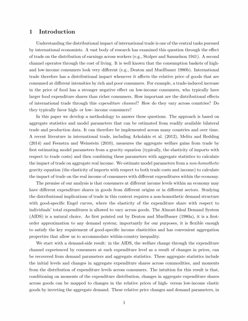
Collecting terms, the welfare change of consumer h is

ωh = W − b× ln(xhx

)+ xh. (14)

Given a distribution of expenditure levels xh across consumers, this expression generates the dis-

tribution of welfare changes in the economy through the expenditure channel.

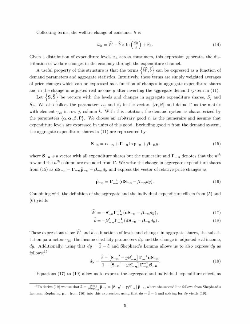
A useful property of this structure is that the termsW , b

can be expressed as a function of

demand parameters and aggregate statistics. Intuitively, these terms are simply weighted averages

of price changes which can be expressed as a function of changes in aggregate expenditure shares

and in the change in adjusted real income y after inverting the aggregate demand system in (11).

Let

S, S

be vectors with the levels and changes in aggregate expenditure shares, Sj and

Sj . We also collect the parameters αj and βj in the vectors α,β and define Γ as the matrix

with element γjk in row j, column k. With this notation, the demand system is characterized by

the parameters α,α,β,Γ. We choose an arbitrary good n as the numeraire and assume that

expenditure levels are expressed in units of this good. Excluding good n from the demand system,

the aggregate expenditure shares in (11) are represented by

S−n = α−n + Γ−n ln p−n + β−ny, (15)

where S−n is a vector with all expenditure shares but the numeraire and Γ−n denotes that the nth

row and the nth column are excluded from Γ. We write the change in aggregate expenditure shares

from (15) as dS−n = Γ−np−n + β−ndy and express the vector of relative price changes as

p−n = Γ−1−n (dS−n − β−ndy) . (16)

Combining with the definition of the aggregate and the individual expenditure effects from (5) and

(6) yields

W = −S′−nΓ−1−n (dS−n − β−ndy) , (17)

b = −β′−nΓ−1−n (dS−n − β−ndy) . (18)

These expressions show W and b as functions of levels and changes in aggregate shares, the substi-

tution parameters γjk, the income-elasticity parameters βj , and the change in adjusted real income,

dy. Additionally, using that dy = x − a and Shephard’s Lemma allows us to also express dy as

follows:15

dy =x− [S−n′ − yβ′−n

]Γ−1−ndS−n

1−[S−n

′ − yβ′−n

]Γ−1−nβ−n

. (19)

Equations (17) to (19) allow us to express the aggregate and individual expenditure effects as

15To derive (19) we use that a ≡ ∂ ln a∂ lnp′−n

p−n =[S−n

′ − yβ′−n

]p−n, where the second line follows from Shephard’s

Lemma. Replacing p−n from (16) into this expression, using that dy = x− a and solving for dy yields (19).

9

function of the level and changes in aggregate expenditure shares, the parameters βj , γjk, the

initial level of adjusted real income, y, and the change in income of the representative consumer, x.

These formulas correspond to infinitesimal welfare changes and can be used to compute a first-order

approximation to the exact welfare change corresponding to a discrete set of price changes.16

In deriving this result, we have not specified the supply-side of the economy, and we have

allowed for arbitrary changes in the distribution of individual expenditure levels, xh. These

demand-side expressions can be embedded in different supply-side structures to study the welfare

changes associated with specific counterfactuals. In the next section, we embed them in a model

of international trade to compute the welfare effects caused by changes in trade costs as function

of observed expenditure shares.

3 International Trade Framework

We embed the results from the previous section in an Armington trade model. Section 3.1

develops a multi-sector Armington model with Almost-Ideal preferences and within-country income

heterogeneity in Section . Section 3.2 derives the non-homothetic gravity equation implied by the

framework. Section 3.3 presents expressions for the welfare changes across households resulting

from foreign shocks.

3.1 Multi-Sector Model

The world economy consists of N countries, indexed by n as importer and i as exporter. Each

country specializes in the production of a different variety within each sector s = 1, .., S, so that

there are J = N×S varieties, each defined by a sector-origin dyad. These varieties are demanded at

different income elasticities. For example, expenditure shares on textiles from India may decrease

with individual income, while shares on U.S. textiles may increase with income. We let psni be the

price in country n of the goods in sector s imported from country i, and pn be the price vector in

country n. The iceberg trade cost of exporting from i to n in sector s is τ sni. Perfect competition

implies that psni = τ snipsii.

Labor is the only factor of production. Country n has constant labor productivity Zsn in sector

s. Assuming that every country has positive production in every sector, the wage per effective unit

of labor in country n is wn = psnnZsn for all s = 1, .., S, and an individual h in country i with zh

effective units of labor receives income of xh = zh×wn. Each country is characterized by a mean zn

and a Theil index Σn of its distribution of effective units of labor across the workforce. Therefore,

the income distribution has mean xn = wnzn and Theil index Σi. Income equals expenditure at

the individual level (and we use these terms interchangeably) and also at the aggregate level due

to balanced trade.

16In assuming that the changes in prices are small, we have not allowed for the possibility that consumers dropvarieties in response to the price changes. When we measure the welfare losses from moving to autarky in theinternational trade setup we account for this possibility.

10

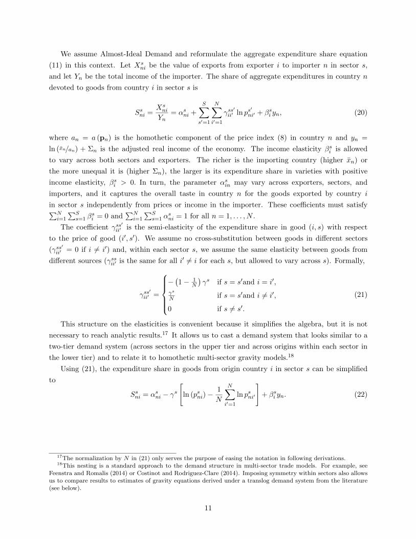
We assume Almost-Ideal Demand and reformulate the aggregate expenditure share equation

(11) in this context. Let Xsni be the value of exports from exporter i to importer n in sector s,

and let Yn be the total income of the importer. The share of aggregate expenditures in country n

devoted to goods from country i in sector s is

Ssni =Xsni

Yn= αsni +

S∑s′=1

N∑i′=1

γss′

ii′ ln ps′ni′ + βsi yn, (20)

where an = a (pn) is the homothetic component of the price index (8) in country n and yn =

ln (xn/an) + Σn is the adjusted real income of the economy. The income elasticity βsi is allowed

to vary across both sectors and exporters. The richer is the importing country (higher xn) or

the more unequal it is (higher Σn), the larger is its expenditure share in varieties with positive

income elasticity, βsi > 0. In turn, the parameter αsin may vary across exporters, sectors, and

importers, and it captures the overall taste in country n for the goods exported by country i

in sector s independently from prices or income in the importer. These coefficients must satisfy∑Ni=1

∑Ss=1 β

si = 0 and

∑Ni=1

∑Ss=1 α

sni = 1 for all n = 1, . . . , N .

The coefficient γss′

ii′ is the semi-elasticity of the expenditure share in good (i, s) with respect

to the price of good (i′, s′). We assume no cross-substitution between goods in different sectors

(γss′

ii′ = 0 if i 6= i′) and, within each sector s, we assume the same elasticity between goods from

different sources (γssii′ is the same for all i′ 6= i for each s, but allowed to vary across s). Formally,

γss′

ii′ =

−(1− 1

N

)γs if s = s′and i = i′,

γs

N if s = s′and i 6= i′,

0 if s 6= s′.

(21)

This structure on the elasticities is convenient because it simplifies the algebra, but it is not

necessary to reach analytic results.17 It allows us to cast a demand system that looks similar to a

two-tier demand system (across sectors in the upper tier and across origins within each sector in

the lower tier) and to relate it to homothetic multi-sector gravity models.18

Using (21), the expenditure share in goods from origin country i in sector s can be simplified

to

Ssni = αsni − γs[

ln (psni)−1

N

N∑i′=1

ln psni′

]+ βsi yn. (22)

17The normalization by N in (21) only serves the purpose of easing the notation in following derivations.18This nesting is a standard approach to the demand structure in multi-sector trade models. For example, see

Feenstra and Romalis (2014) or Costinot and Rodriguez-Clare (2014). Imposing symmetry within sectors also allowsus to compare results to estimates of gravity equations derived under a translog demand system from the literature(see below).

11

The corresponding expenditure share for consumer h in goods from country n in sector s is

ssni,h = αsni − γs[

ln (psni)−1

N

N∑i′=1

ln psni′

]+ βsi

(ln

(xhxn

)+ yn

). (23)

Adding up (22) across exporters, the share of sector s in the total expenditures of country n is:

Ssn =

N∑i=1

Ssni = αsn + βsyn, (24)

where

αsn =N∑i=1

αsni,

βs

=

N∑i=1

βsi .

In turn, the share of sector s in total expenditures of consumer h is

ssn,h =N∑i=1

ssni,h = αsn + βs(yn + ln

(xhxn

)). (25)

Equations (24) and (25) show that the expenditure shares across sectors have an “extended

Cobb-Douglas” form, which allows for non-homotheticities across sectors through βs

on top of the

fixed expenditure share αsn. We refer to βs

in (24) as the “sectoral betas”.19

3.2 Non-Homothetic Gravity Equation

The model yields a sectoral non-homothetic gravity equation that depends on aggregate data

and the demand parameters. These parameters are the elasticity of substitution γs across exporters

in sector s and the income elasticity of the goods supplied by each exporter in each sector, βsn.Combining (22) and the definition of yn gives

Xsni

Yn= αsni − γs ln

(τ snip

sii

τ snps

)+ βsi

[ln

(xn

a (pn)

)+ Σn

], (26)

where

τ sn = exp

(1

N

N∑i=1

ln (τ sni)

)

19If βs

= 0 for all s (so that non-homotheticities across sectors are shut down), sectoral shares by importer areconstant at Ssn = αsn, as it would be the case with Cobb-Douglas demand across sectors.

12

and

ps = exp

(1

N

N∑i=1

ln (psii)

).

Income of each exporter i in sector s equals the sum of sales to every country, Y si =

∑Nn=1X

sni.

Using this condition and (26) we can solve for γs ln (psii/ps). Replacing this term back into (26),

import shares in country n can be expressed in the gravity form:

Xsni

Yn= Asni +

Y si

YW− γsT sni + βsiΩn, (27)

where YW =∑I

i=1 Yi stands for world income, and where

Asni = αsni −N∑

n′=1

(Yn′

YW

)αsn′i, (28)

T sni = ln

(τ sniτ sn

)−

N∑n′=1

(Yn′

YW

)ln

(τ sn′iτ sn′

), (29)

Ωn =

[ln

(xnan

)+ Σn

]−

N∑n′=1

(Yn′

YW

)[ln

(xn′

an′

)+ Σn′

]. (30)

The first term in (27), Asni, captures cross-country differences in tastes across sectors or ex-

porters; this term vanishes if αsni is constant across importers n. The second term, Y si /YW , captures

relative size of the exporter due to, for example, high productivity relative to other countries. The

third term, T sni, measures both bilateral trade costs and multilateral resistance (i.e., the cost of

exporting to third countries).

The last term in (27), βsiΩn, is the non-homothetic component of the gravity equation. It

includes the good-specific Engel curves needed to measure the unequal gains from trade across

consumers. This term captures the “mismatch” between the income elasticity of the exporter

and the income distribution of the importer. The larger Ωn is, either because average income or

inequality in the importing country n are high relative to the rest of the world, the higher is the

share of expenditures devoted to goods in sector s from country i when i sells high income-elastic

goods (βsi > 0). If non-homotheticities are shut down, this last terms disappears and the gravity

equation in (27) becomes the translog gravity equation.

3.3 Distributional Impact of a Foreign-Trade Shock

Using the results from Section 2, we derive the welfare impacts of a foreign-trade shock across

the expenditure distribution. Without loss of generality we normalize the wage in country n to 1,

wn = 1. Consider a foreign shock to this country consisting of an infinitesimal change in foreign

productivities, foreign endowments or trade costs between any country pair. From the perspective

of an individual consumer h in country n, this shock affects welfare through the price changes

13

psnii,s and the income change xh. From (21) and (22), the change in the price of imported relative

to own varieties satisfies:

psni − psnn = −dSsni − dSsnnγs

+1

γs(βsi − βsn) dyn. (31)

Because only foreign shocks are present, the change in income xh is the same for all consumers

and equal to the change in the price of domestic commodities, xh = x = psnn = 0 for all h in country

N and for all s = 1, .., S.20 Imposing these restrictions, we can re-write (17) as

Wn ≡ WH,n + WNH,n, (32)

where

WH,n =S∑s=1

N∑i=1

1

γsSsni (dSsni − dSsnn) , (33)

WNH,n =S∑s=1

N∑i=1

1

γsSsni (βsn − βsi ) dyn. (34)

Using these restrictions, we can also rewrite the slope of the individual effect in (18) as

bn =

S∑s=1

N∑i=1

βsiγs

(dSsnn − dSsni + (βsi − βsn) dyn) , (35)

and the change in the adjusted real income from equation (19) as

dyn =

∑Ss=1

∑Ni=1

1γs (Ssni − βsniyn) (dSsni − dSsnn)

1−∑S

s=1

∑Ni=1

1γs (Ssni − βsi yn) (βsn − βsi )

. (36)

Expressions (32) to (36) provide a closed-form characterization of the welfare effects of a foreign-

trade shock that includes three novel margins. First, preferences are non-homothetic with good-

specific income elasticities. Second, the formulas accommodate within-country inequality through

the Theil index of expenditure distribution Σn, which enters through the level of yn. Third, and

key for our purposes, the expressions characterize the welfare change experienced by individuals at

each income level, so that the entire distribution of welfare changes across consumers h in country

n can be computed from (14) using:

ωh = Wn − bn × ln(xhx

). (37)

The aggregate expenditure effect, Wn, includes a homothetic part WH,n independent from the

βsn’s. When non-homotheticities are shut down, this term corresponds to the aggregate gains under

20Note that because of the Ricardian supply-side specification there is no change in the relative price acrossdomestic goods or in relative incomes across consumers.

14

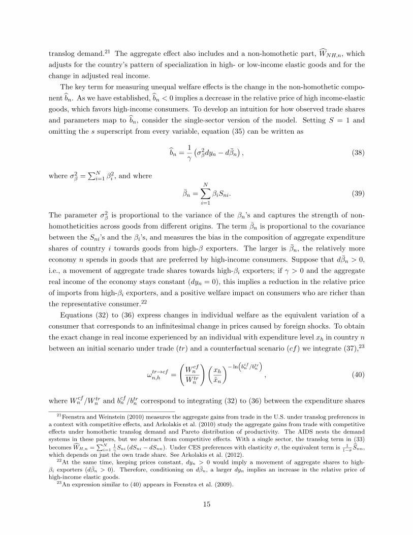
translog demand.21 The aggregate effect also includes and a non-homothetic part, WNH,n, which

adjusts for the country’s pattern of specialization in high- or low-income elastic goods and for the

change in adjusted real income.

The key term for measuring unequal welfare effects is the change in the non-homothetic compo-

nent bn. As we have established, bn < 0 implies a decrease in the relative price of high income-elastic

goods, which favors high-income consumers. To develop an intuition for how observed trade shares

and parameters map to bn, consider the single-sector version of the model. Setting S = 1 and

omitting the s superscript from every variable, equation (35) can be written as

bn =1

γ

(σ2βdyn − dβn

), (38)

where σ2β =

∑Ni=1 β

2i , and where

βn =

N∑i=1

βiSni. (39)

The parameter σ2β is proportional to the variance of the βn’s and captures the strength of non-

homotheticities across goods from different origins. The term βn is proportional to the covariance

between the Sni’s and the βi’s, and measures the bias in the composition of aggregate expenditure

shares of country i towards goods from high-β exporters. The larger is βn, the relatively more

economy n spends in goods that are preferred by high-income consumers. Suppose that dβn > 0,

i.e., a movement of aggregate trade shares towards high-βi exporters; if γ > 0 and the aggregate

real income of the economy stays constant (dyn = 0), this implies a reduction in the relative price

of imports from high-βi exporters, and a positive welfare impact on consumers who are richer than

the representative consumer.22

Equations (32) to (36) express changes in individual welfare as the equivalent variation of a

consumer that corresponds to an infinitesimal change in prices caused by foreign shocks. To obtain

the exact change in real income experienced by an individual with expenditure level xh in country n

between an initial scenario under trade (tr) and a counterfactual scenario (cf) we integrate (37),23

ωtr→cfn,h =

(W cfn

W trn

)(xhxn

)− ln(bcfn /b

trn

), (40)

where W cfn /W tr

n and bcfn /btrn correspond to integrating (32) to (36) between the expenditure shares

21Feenstra and Weinstein (2010) measures the aggregate gains from trade in the U.S. under translog preferences ina context with competitive effects, and Arkolakis et al. (2010) study the aggregate gains from trade with competitiveeffects under homothetic translog demand and Pareto distribution of productivity. The AIDS nests the demandsystems in these papers, but we abstract from competitive effects. With a single sector, the translog term in (33)

becomes WH,n =∑Ni=1

1γSni (dSni − dSnn). Under CES preferences with elasticity σ, the equivalent term is 1

1−σ Snn,which depends on just the own trade share. See Arkolakis et al. (2012).

22At the same time, keeping prices constant, dyn > 0 would imply a movement of aggregate shares to high-βi exporters (dβn > 0). Therefore, conditioning on dβn, a larger dyn implies an increase in the relative price ofhigh-income elastic goods.

23An expression similar to (40) appears in Feenstra et al. (2009).

15

in the initial and counterfactual scenarios. If ωtr→cfn,h < 1, individual h is willing to pay a fraction

1− ωtr→cfn,h of her income in the initial trade scenario to avoid the movement to the counterfactual

scenario.

In Section 5 we perform the counterfactual experiment of bringing each country to autarky, and

also simulate partial changes in the trade costs. In each case, we compute (40) using the changes in

expenditure shares that take place between the observed and counterfactual scenarios. For that, we

need the income elasticities βsn and the substitution parameters γs. The next section explains

the estimation of the gravity equation to obtain these parameters.

4 Estimation of the Gravity Equation

In this section, we estimate the non-homothetic gravity derived in Section 3.24 Section 4.1

describes the data, and Section 4.2 presents the estimation results.

4.1 Data

To estimate the non-homothetic gravity equation we use data compiled by World Input-Output

Database (WIOD). The database records bilateral trade flows and production data by sector for

40 countries (27 European countries and 13 other large countries) across 35 sectors that cover

food, manufacturing and services (we take an average of flows between 2005-2007 to smooth out

annual shocks). The data record total expenditures by sector and country of origin, as well as final

consumption; we use total expenditures as the baseline and report robustness checks that restrict

attention to final consumption. We obtain bilateral distance, common language and border infor-

mation from CEPII’s Gravity database. Price levels, adjusted for cross-country quality variation,

are obtained from Feenstra and Romalis (2014). Income per capita and population are from the

Penn World Tables, and we obtain gini coefficients from the World Income Inequality Database

(Version 2.0c, 2008) published by the World Institute for Development Research.25

The left-hand-side of (27),XsniYi

, can be directly measured using the data from sector s and

exporter i’s share in country n’s expenditures. Similarly, we use country i’s sales in sector s to

constructY siYW

.

The term T sni in (27) captures bilateral trade costs between exporter i and importer n in sector

s relative to the world. Direct measures of bilateral trade costs across countries are unavailable so

we proxy them with bilateral observables. Specifically we assume τ sni = dρs

niΠjg−δsjj,ni ε

sni, where dni

stands for distance, ρs reflects the elasticity between distance and trade costs in sector s, the g’s

24In principle, one could obtain the parameters from other data sources, such as household surveys, that recordconsumption variation across households within countries. We have chosen to use cross-country data because it isinternally consistent within our framework, and it is a common approach taken in the literature. In Section 5.4, weexplore results that use parameters estimated from the U.S. consumption expenditure microdata.

25The World Income Inequality Database provides gini coefficients from both expenditure and income data. Ideally,we would use ginis from only the expenditure data, but this is not always available for some countries during certaintime periods. We construct a country’s average gini using the available data between 2001-2006.

16

are other gravity variables (common border and common language),26 and εsni is an unobserved

component of the trade cost between i and n in sector s.27 This allows us to re-write the gravity

equation as

Xsni

Yn= Asni +

Y si

YW− (γsρs)Dni +

∑j

(γsδsj

)Gj,ni + βsiΩn + εsni, (41)

where, letting dn = 1N

∑Ni=1 ln (dni) ,

Dni = ln

(dnidn

)−

N∑n′=1

(Yn′

YW

)ln

(dn′idn′

). (42)

and where Gj,ni is defined in the same way as 42 but with gj,ni instead of dni.28 As seen from (45),

because we do not directly observe trade costs we cannot separately identify γs and ρs. Following

Novy (2012) we set ρs = ρ = 0.177 for all s.29

The term Ωn in (41) captures importer n’s inequality-adjusted real income relative to the

world. To construct this variable, we assume that the distribution of efficiency units in each

country n is log-normal, ln zh ∼ N(µn, σ

2n

). This implies a log-normal distribution of expenditures

with Theil index equal to σ2n/2 where σ2

n = 2[Φ−1

(ginin+1

2

)]2. We construct xn from total

expenditure and total population of country n. We follow Deaton and Muellbauer (1980a), and

more recently Atkin (2013), to proxy the homothetic component an with a Stone index, for which

we use an =∑

i Sni ln (pnndρni), where pnn are the quality-adjusted prices estimated by Feenstra

and Romalis (2014). The obvious advantage of this approach is that it avoids the estimation of

the αsni, which enter the gravity specification non-linearly and are not required for our welfare

calculations. The measure of real spending per capita divided by the Stone price index, xi/ai, is

strongly correlated with countries’ real income per capita; this suggests that Ωi indeed captures

the relative difference in real income across countries.

To measure Asni, we decompose αsni into an exporter effect αi, a sector-specific effect αs, and an

importer-specific taste for each sector εsn:

αsni = αi (αs + εsn) . (43)

We further impose the restriction∑N

i=1 αi = 1. Under the assumption (43), the sectoral expenditure

26Since bilateral distance is measured between the largest cities in each country using population as weights, it isdefined when i = n; see Mayer and Zignago (2011). Note that we parametrize trade costs such that a positive effectof common language and common border on trade is reflected in δsj > 0.

27Waugh (2010) includes exporter effects in the trade-cost specification. The gravity equation (27) would beunchanged in this case because the exporter effect would wash out from T sni in (29).

28From the structure of trade costs it follows that the error term is εsni = −γs(

ln(εsni

εsn

)−∑Nn′=1

(Yn′YW

)ln

(εsn′iεsn′

))where εsn = exp

(1N

∑Nn′=1 ln (εsn′i)

).

29Below we explore the sensitivity of the results to alternative values of this parameter.

17

shares from the upper-tier equation (24) becomes:

Ssn = αs + βsyn + εsn. (44)

This equation is an Engel curve that projects expenditure shares on the adjusted real income.30

Specifically, it regresses sector expenditure shares on sector dummies and the importer’s ad-

justed real income interacted with sector dummies. The interaction coefficients will have the

structural interpretation as the sectoral betas βs.31 Using (28), (43), and (44) we can write

Asni = αi

(Ssn − SsW − β

sΩn

), where SsW is the share of sector s in world expenditures. Combining

this with the gravity equation in (41), we reach the following estimating equation:

Xsni

Yn=Y si

YW+ αi (Ssn − SsW )− (γsρs)Dni +

∑j

(γsδsj

)Gj,ni +

(βsi − αiβs

)Ωn + εsni, (45)

The gravity equation (45) identifies(βsi − αiβs

)using the variation in Ωn across importers for

each exporter. Using the βs estimated from the sectoral Engel curve in (44) and the αi estimated

from (45) we can recover the βsi (which is needed to perform the counterfactuals). Since the market

shares sum to one for each importer, it is guaranteed that∑

i

∑s β

si = 0 in the estimation, as

the theory requires. We cluster the estimation at the importer level to allow for correlation in the

errors across exporters.

The sectoral gravity equation aggregates to the gravity equation of a single-sector model. Sum-

ming (45) across sectors s gives the total expenditure share dedicated to goods from i in the

importing country n,

Xni

Yn=

YiYW− (γρ)Dni +

∑j

(γδj)Gj,ni + βiΩn + εni, (46)

where γρ ≡∑S

s=1 γsρs, βi ≡

∑Ss=1 β

si , and εni ≡

∑Ss=1 ε

sni. We can readily identify (46) as the

gravity equation that would arise in a single-sector model (S = 1). Thus, summing our estimates on

the gravity terms from (45) will match the gravity coefficients from a single-sector model. Likewise,

the sum of the sector-specific income elasticities by exporter∑

s βsi estimated from (45) matches

the income elasticity βi estimated from (46).

30Note that sectoral shares in value added and efficiency units are allowed to vary independently from expenditureshares depending on the distribution of sectoral productivities Zsn and trade patterns. The sectoral productivities arenot estimated and are not needed to perform the counterfactuals.

31The term εsi captures cross-country differences in tastes across sectors that are not explained by differences inincome or inequality levels. As in Costinot et al. (2012) or Caliendo and Parro (2012), this flexibility is needed forthe model to match sectoral shares by importer. This approach to measuring taste differences is also in the spirit ofAtkin (2013), who attributes regional differences in tastes to variation in demand that is not captured by observables.

18

4.2 Estimation Results

We begin by estimating the single-sector gravity model in equation (46). This regression ag-

gregates across the sectors in the data, and as illustrated in (46), the baseline multi-sector gravity

equation aggregates exactly to this single-sector gravity equation. The results are reported in Table

1. Consistent with the literature, we find that bilateral distance reduces trade flows between coun-

tries, which is captured by the statistically significant coefficient on Dni. Under the assumption

that ρ = 0.177, the estimate implies γ = 0.24 (=.043/.177).32 The additional trade costs–common

language and a contiguous border term–also have the intuitive signs.

The table also reports estimates of the 40 βi parameters, one corresponding to each exporter, in

the subsequent rows. The exporters with the highest β’s are the U.S. and Japan, while Indonesia

and India have the lowest β’s. This means that U.S. and Japan export goods that are preferred by

richer consumers, while the latter export goods that are preferred by poorer consumers. To visualize

the β’s, we plot them against the per capita income in Figure 1. The relationship is strongly positive

and statistically significant. We emphasize that this relationship is not imposed by the estimation.

Rather, these coefficients reflect that richer countries are more likely to spend on products from

richer countries, conditional on trade costs. We also note that the β’s are fully flexible, which is

why the coefficients are often not statistically significant, but the null hypothesis that all income

elasticities are zero is rejected.33 Moreover, the finding that a subset are statistically significant is

sufficient to reject homothetic preferences in the data, and is consistent with the existing literature

who finds that richer countries export goods with higher income elasticities.34

We next report the results for the multi-sector estimation. As noted earlier, the analysis in-

volves estimating the Engel curve in (44), which projects sectoral expenditure shares on adjusted

real income across countries. Table 2 reports the sectoral betas, βs. Compared to food and manu-

facturing sectors (listed in column 1A), service sectors (listed in column 1B) tend to be high-income

elastic.35 This pattern can be visualized by plotting countries’ expenditure shares in these three

broad categories against their income per capita in Figure 2: the Engel curve for services is posi-

tively sloped, while it is negatively sloped for food and manufacturing.36 These sectoral elasticities

32This estimate is close to the translog gravity equation estimate of γ = 0.167 estimated by Novy (2012). Feenstraand Weinstein (2010) report a median γ of 0.19 using a different data, level of aggregation and estimation procedure,so our estimate is in line with the few papers that have run gravity regressions with the translog specification.

33If we reduce the number of estimated parameters by imposing a relationship between income elasticities andexporter income, we find a positive and statistically significant relationship between the two variables. Specifically, wecan impose that βi = B0 +B1yi, which is similar to how Feenstra and Romalis (2014) allow for non-homotheticities.The theoretical restriction

∑i βi = 0 implies that B0 = −B1

1N

∑i yi, transforming this linear relationship to βi =

B1

(yi − 1

N

∑i′ yi′

)and reducing the number of income elasticity parameters to be estimated from 40 to 1. If we

impose this to estimate the gravity equation, we find B1 = 0.0057 (standard error of 0.0026). This estimate is veryclose to regressing our estimated βi’s reported in Table 1 on

(yi − 1

N

∑i′ yi′

), which yields a coefficient of 0.008

(standard error of 0.0035).34See Hallak (2006), Khandelwal (2010), Hallak and Schott (2011), and Feenstra and Romalis (2014).35To see this, we aggregate the βs into three categories: food includes “Agriculture” and “Food, Beverages and

Tobacco”, manufacturing includes the remaining sectors listed in column 1A of Table 2, and services is comprised ofthe 19 sectors in column 1B. The corresponding elasticities for food, manufacturing and services are -0.0343, -0.0410,and 0.0753, respectively. (Again, the sum of these three broad classifications is zero.)

36This is consistent with the literature on structural transformation; see Herrendorf et al. (2014).

19

are highly correlated with sectoral elasticities estimated using a different non-homothetic frame-

work on different data by Caron et al. (2014); see Appendix Figure A.1 which plots the two sets of

elasticities against each other.37

The results of the sectoral gravity equation in (45) is reported in Table 3. Columns 1A and 1B

report the 35 sector-specific distance coefficients, ργs (where ρ = .177 as before). Recall, these these

coefficients sum to coefficient on distance from the single-sector model (See Table 1). Likewise, the

sector-specific language and border coefficients in columns 2 and 3 of Table 3 sum exactly to the

corresponding coefficients in the single-sector estimation.

We suppress the estimates of βsn for readability purposes, but recall that∑

s βsi equals the

exporter income elasticities βi reported in the single-sector gravity equation. Also note that by

construction,∑

n βsn equals the sectoral elasticities β

sdisplayed in Table 2. To see how βsn relate

to exporter income per capita, we aggregate these coefficients to three broad classifications–food,

manufacturing and services–and report the plot in Figure 3. Analogous to the single-sector esti-

mates in Figure 1, we find that the positive relationship between exporter income per capita and

income elasticities holds within sectors as well.

5 The Unequal Gains from Trade

This section conducts counterfactual analyses to measure the distributional consequences of

trade. Section 5.1 explains how we numerically implement the expressions from Section 3.3. Section

5.2 shows the results of autarky counterfactuals in the single-sector version of our model. Section 5.3

presents the main results: the autarky counterfactuals in the baseline multi-sector model. Section

5.4 presents a series of robustness checks. In Section 5.5, we conduct counterfactuals of partial

changes in foreign trade costs.

5.1 Computing Consumer-Specific Welfare Changes

To measure the unequal distribution of the gains from trade across consumers, we perform the

counterfactual experiment of changing trade costs. The main results bring consumers in each coun-

try to autarky, and we also simulate partial changes in trade costs. Because we know the changes

in expenditure shares that take place between the observed trade shares and the counterfactual

scenarios, we can use the results from Section 3.3 to measure the welfare change experienced by

consumers at each income level. But before applying these results, a few considerations are in

order.

First, we highlight that throughout the analysis we take as given the specialization pattern of

countries across goods with different income elasticity. That is, the βsn are not allowed to change

in counterfactual scenarios. These patterns could change as trade costs change, but we note that

37Caron et al. (2014) estimate sectoral income elasticities on GTAP data using constant relative income preferences.We match GTAP sector classifications with WIOD sector classifications to produce the scatter plot.

20

the direction of the change will depend on what forces determine specialization across goods with

different income elasticity.38

Second, the restriction to non-negative individual expenditure shares may bind in some in-

stances. Therefore, to compute expression (40) for the welfare change ωtr→cfn,h of each consumer

h from country n between the initial scenario under trade (tr) and each counterfactual scenario

(cf), we must first compute consumer-specific reservation prices. Following Feenstra (2010), this

amounts to setting the individual expenditure shares of dropped varieties to zero according to (23),

and substituting reservation prices back into the consumed varieties. We then numerically integrate

equations (32) to (36) between the aggregate expenditure shares for country n in (22) evaluated

at those reservation prices. As this procedure is done for each consumer h separately, we add a

subscript h to the terms in (40) to denote that the aggregate expenditure shares used to construct

the welfare change of each consumer are consumer-specific:

ωtr→cfn,h =

(W cfn,h

W trn,h

)(xhxn

)− ln(bcfn,h/b

trn,h

). (47)

We describe these steps formally in Appendix A.

Finally, we assume, as with the gravity estimation, that the expenditure distribution in country

n is lognormal with variance σ2n. This allows mapping the observed gini coefficient to the Theil

index. Henceforth, we index consumers by their percentile in the income distribution, so that

h ∈ (0, 1). Under the log-normal distribution, the expenditure level of a consumer at percentile h

in country i is ezhσi+µi , where zh denotes the value from a standard normal z-table at percentile h,

and xi = eσi+µi . We can therefore re-write (47) as:

ωtr→cfn,h =

(W cfn,h

W trn,h

)(bcfn,hbtrn,h

)σn(1−zh)

. (48)

Consumers at percentile h are willing to pay a fraction 1 − ωtr→cfn,h of their income under trade to

avoid the movement from the trade to the counterfactual scenario when ωtr→cfn,h < 1.

5.2 Single-Sector Analysis

To convey some intuition, we first report results from the single-sector version of the model

using the parameters from Table 1. Figure 4 plots the gains from trade by percentile of the income

distribution for all the countries in our data (i.e., it plots 1− ωtr→cfn,h for ωtr→cfn,h defined in (48) for

all n and h = 0.01, .., 0.99 when each country is moved to autarky). To facilitate the comparisons

across countries, we express the gains from trade of each percentile as difference from the gains

38If specialization is demand-driven by home-market effects, as in Fajgelbaum et al. (2011), poor countries wouldspecialize less in low-income elastic goods as trade costs increase. However, if specialization is demand-driven in aneoclassical environment as in Mitra and Trindade (2005), or determined by relative factor endowments, as in Schott(2004) or Caron et al. (2014), the opposite would happen. To our knowledge, no study has established the relativeimportance of these forces for international specialization patterns in goods with different income elasticity.

21

of the 50th percentile in each country. The solid red line in the figure shows the average for each

percentile across the 40 countries in our sample.

The typical U-shape relationship between the gains from trade and the position in the income

distribution implies that poor and rich consumers within each country tend to reap larger benefits

from trade compared to middle-income consumers. The reason for these patterns is intuitive in the

light of the earlier discussion of equation (38) for the change in the relative price of high-income

elastic goods. In a movement to autarky, the change in the relative price of high income-elastic

goods experienced by the representative agent of country n is:

ln

(bcfnbtrn

)=

1

γ

(σ2β

(ycfn − ytrn

)−(βn − βn

)). (49)

The formula reveals that a key determinant of the bias of trade is the income elasticity of each

country’s exports relative to each country’s imports, captured by βn − βn.39 A positive βn − βnimplies that expenditures move towards higher income elastic goods in a movement to autarky,

potentially implying a reduction in their relative price. Therefore, for low-income (high-income)

countries which tend to be exporters of low (high) income-elastic goods as shown in Figure 1,

trade openness relatively favors rich (poor) individuals.40 In countries that export products with

intermediate income elasticities, middle-income consumers benefit the least from trade because

their home country already supplies these goods; at the same time, opening to trade supplies both

the rich and poor with products that better match their tastes. This creates a U-shaped pattern

of the gains from trade for the typical country in the single-sector model.

5.3 Multi-Sector Analysis

We now present the baseline results from the multi-sector model. We first report the aggregate

gains from trade, defined as the gains for the representative agent in each country. Columns 1A

and 1B of Table 4 report the real income loss for the representative consumer in each country.41

We compare these results to a homothetic case by setting βsn = 0 for all n and s in the gravity

estimation and re-estimating the remaining parameters; this amounts to estimating a translog

multi-sector gravity equation. The translog gravity estimates are reported in Appendix Table A.1;

the results reveal that the estimated gravity coefficients hardly change under the constraint that

preferences are homothetic (compare Table 3 with Appendix Table A.1). As a result, the aggregate

gains under the translog specification, reported in Columns 2A and 2B of Table 4, are very similar

to the aggregate gains under the non-homothetic AIDS. This suggests that, in our context, non-

39A decomposition of (49) reveals that the second term inside the parenthesis accounts for majority of the variation,80.7 percent. The first term accounts for only 13.9 percent, and the covariance for the remaining 5.4 percent.

40When the economy is in autarky, all foreign goods are dropped and demand for the domestic variety correspondsto a single-good AIDS with unitary income elasticity; see Feenstra (2010). However, the parameter βn still enters in(49) because it measures the difference in relative prices between the actual trade scenario and the autarky prices.

41The aggregate gains from trade in the multi-sector setting are higher than the single-sector case. This is consistentwith Ossa (2015) and Costinot and Rodriguez-Clare (2014) who show that allowing for sectoral heterogeneity leadsto larger measurement of the aggregate gains from trade in CES environments.

22

homotheticities do not fundamentally change the estimates of the aggregate gains from trade.42

However, as we discuss next, they have a strong impact on the bias of the gains from trade across

consumers.

Figure 5 reports the unequal gains from trade with multiple sectors across percentiles using the

parameters from Tables 2 and 3. As before, the figure shows the gains from trade for each percentile

in each country as a difference from the median percentile of each country. Table 5 reports the

absolute gains from trade at the 10th, median, and 90th percentile, as well as for the representative

consumer of each country (which is identical to Column 1 of Table 4).

There are two important differences between the results under the single- and under the multi-

sector frameworks. First, the relative effects across percentiles are considerably larger. In the

single-sector case from Figure 4, the gains from trade (relative to the median) lie within the -5

percent to 10 percent band across most countries and percentiles, while in the multi-sector case the

range increases to -40 percent to 60 percent. Second, poor consumers are now predicted to gain

more from trade than rich consumers in every country. Every consumer below the median income

gains more from trade than every consumer above the median. On average across the countries in

our sample, the gains from trade are 63 percent at the 10th percentile of the income distribution

and 28 percent at the 90th percentile.

Why do the results for the multi-sector analysis differ from the single-sector analysis? The

multi-sector model allows for two key additional margins that influence the pro-poor bias of trade:

heterogeneity in the elasticity of substitution γs and in the sectoral betasβs

. By construction,

if we restricted the γs and βsn to be constant across sectors in the multi-sector estimation, we

would recover the same unequal gains from trade as in the single-sector estimation, and Figure 5

would look identical to Figure 4. To gauge the importance of each of these margins in shaping

the unequal gains, Figure 6 shows the average gains from trade by percentile across all countries

for four models: 1) the single-sector model (which is equal to the solid red curve in Figure 4);

2) a multi-sector model with homothetic sectors that imposes βs = 0 for all s but allows for

heterogeneous γ’s; 3) a multi-sector model that imposes symmetric γ’s (γs = 1J γ) but allows for

non-homothetic sectors; and 4) the baseline multi-sector model that allows for non-homothetic

sectors and sector-specific γ′s (which is equal to the solid red curve in Figure 5).

We find that including non-homotheticities across sectors (i.e., comparing models 1 versus 3

or models 2 versus 4) is crucial for the strongly pro-poor bias of trade. The reason is that low-

income consumers spend relatively more on sectors that are more traded, whereas high-income

consumers spend relatively more on services, which are among the least internationally traded

sectors. Recall from Figure 2 that the income elasticities of the service sectors are higher than

non-service sectors; in addition, the average import share among the service sectors is 6.4 percent

compared to 20 percent and 48 percent for food and manufacturing sectors, respectively. We also

42We note that this statement relies on defining the aggregate gains as those of the representative consumer.An alternative, which we do not pursue here, would be to define the aggregate gains as the average change in realincome, 1

H

∑h ω

tr→cfn,h xh. This would correspond to the amount of income per capita needed to leave every consumer

indifferent between trade and autarky.

23

find that including heterogeneity in γs across sectors (i.e., comparing models 1 versus 2, or models

3 versus 4) slightly biases the gains from trade towards poor consumers. The reason is that low-

income consumers concentrate spending on sectors with a lower substitution parameter γs. To see

this, we construct, for each percentile in each country, an expenditure-share weighted average of the

sectoral gammas. Then, we average across all countries and report the results in Appendix Figure

A.2. The figure reveals that higher percentiles concentrate spending in sectors where exporters sell

more substitutable goods. In sum, larger expenditures in more tradeable sectors and a lower rate

of substitution between imports and domestic goods lead to larger gains from trade for the poor

than the rich.

While the gains from trade are larger for the poor in every country, we also observe cross-country

heterogeneity in the difference between the gains from trade of poor and rich consumers. What

determines the strength in the pro-poor bias of trade? As in the single-sector case the answer lies

in part in the income elasticity of each country’s products vis-a-vis its natural trade partners. In

countries that export relatively low income-elastic goods, such as India, the gains from trade are

relatively less biased to poor consumers. In these countries, opening to trade increases the relative

price of low-income elastic goods (which are exported), or decreases that of high-income elastic

goods (which are imported). This can be seen in Figure 7, which plots the difference between

the gains from trade of the 90th and 10th percentiles against each country’s income elasticity

(βn =∑

s βsn). The difference between the gains from trade of the 90th and 10th percentiles is

more negative in countries with higher income elasticity of exports. However, the income elasticity

of the goods exported by each country is not sufficient to determine the bias of trade, which also

depends on the distribution of expenditures across goods with different income elasticity, as implied

by (35).43

5.4 Robustness

This subsection examines the robustness of our baseline results to alternative specifications.

5.4.1 Sectoral Income Elasticities βs

The first set of robustness checks examines the robustness of estimating the βs

using the Engel

curve regression in (44).

An assumption in our framework is that individual preferences are identical across countries.44

This assumption is standard in models of international trade and in quantitative analyses of these

models. A second assumption, that results from the structure of the price elasticities in (21), is that

relative prices do not affect sectoral expenditure shares in (44) other than through the homothetic

component a(p) (and only so if non-homotheticities are present). As a result, equation (44) for

43If the U.S. and India are excluded from the figure, the relationship remains negative but not significant. Thissuggests that although the income elasticity of a country’s products matters, the other terms in (35) also influencethe overall bias of trade.

44Note that we do allow for some heterogeneity in preferences across countries through the parameter αsin, whichis reflected in the term εsn of the Engel curve (44).

24

the aggregate shares has an “extended Cobb-Douglas” form consisting of a constant plus a slope

with respect to income. This property of the model is also similar to the majority of multi-sector

trade models that assume Cobb-Douglas preferences across sectors. Our approach to estimating

the Engel curves using cross-country data is consistent with these assumptions. Under these two

assumptions, the slopes of Engel curves across consumers within a country are the same as the

slopes of the Engel curves that we estimate using aggregate data across countries. This motivates

the following two robustness checks.

First, we re-estimate the Engel curve slopes from equation (44) using variation over time by

including country-sector fixed effects, rather than just sector fixed effects. This specification controls

for time invariant differences in country characteristics, and in principle, may result in very different

estimates of the βs

parameters.45 However, the βs

estimated using the specification with country-

sector fixed effects are positively correlated with the baseline estimates (the correlation between

the estimates is 0.68). Figure 8 compares the welfare gains, averaged across countries, using these

alternative sectoral elasticities with the baseline results, resulting in very similar patterns.

As a second robustness check, we estimate the sectoral elasticities relying on consumer-level

microdata. This check addresses the concern that variation in consumer expenditures within coun-

tries may not be accurately reflected in aggregate expenditures across countries.46 We use the 2013

U.S. Consumer Expenditure Survey (CE) microdata that records expenditures to estimate the βs

from the consumer-level version of (44) implied by the model,47

ssn,h = ζsn + βs

ln (xh) + εsn,

where ζsn ≡ αs − βs

ln (an) and h refers to a household in the CE data. To cleanly map the

categories in the CE with the sectors in the aggregate data, we classify household expenditures

into three broad categories—food, manufacturers and services.48 We find βfood,CE

= −0.057 (s.e.

= 0.00009), βmfg,CE

= 0.0375 (s.e. = 0.0012), and βservice,CE

= 0.0197 (s.e.=0.001). Compared

to baseline Engel curves, the microdata reveal a positive income elasticity for manufactures, and

a somewhat flatter (though still positive) income elasticity for services. We then re-estimate the

remaining parameters of the model from the gravity equation in (27) imposing these sectoral betas,

and recompute the gains from trade using the same aggregate data as in the baseline case.

The results are presented in Figure 8. Consistent with the baseline results, the poorest con-

sumers gain more from trade than the median. The reason is that in both the CE and aggregate

45We use an average of bilateral flows between 1995-1997 as the initial year to smooth out annual shocks.46For example, Bee et al. (2012) discusses inconsistencies between aggregation of consumer expenditure surveys

and national accounts data in the U.S.47If the CE recorded expenditures by country of origin and/or prices, it would be possible to use these data to

estimate obtain estimates of βsn and/or γs.48We use the 2013 quarterly-level summary expenditure files: fmli132.dta, fmli133.dta, fmli134.dta, and

fmli141.dta. We analyze consumption in the current quarter, and construct the categories as follows. Food isthe sum of foodcq alcbevcq, tobacccq. Manufactured goods is the sum of apparcq, cartkncq, cartkucq, othvehcq,gasmocq, tvrdiocq, otheqcq, predrqcq, medsupcq, houseqcq, misccq. Services is the sum of vehfincq, mainrpcq,vehinscq, vrntlocq, pubtracq, feeadmcq, hlthincq, medsrvcq, sheltcq, utilcq, housopcq, perscacq, readcq, educacq,cashcocq, perinscq.

25

data, the Engel curve on food sectors is negative and has low γs. The main difference is revealed

at the top of the expenditure distribution. In the baseline results, we generally find that the rich

gain less than the median-income consumer. But when we estimate the sectoral income elasticities

using the the CE data, the average curve bends upward at higher income levels. This is because

manufacturing sectors have a higher income elasticity in the CE data and are also more tradeable

(relative to services). As a result, using sectoral income elasticities from microdata reveals a slightly

different bias of trade relative to the baseline case.

5.4.2 Price Elasticity of Service Sectors and Non-Tradeability

The second set of robustness checks alter the assumptions on the degree of tradeability of

some of the service sectors in the data. As discussed earlier, the high elasticity parameters γs in

service sectors partly affect the bias of the unequal gains. These parameters were obtained by first

identifying ρsγs from the semi-elasticity of trade with respect to distance in the gravity equation

45, and then setting ρs = 0.177 for all sectors. However, one might expect ρs to be higher for some

service sectors that are essentially non-traded, which would lead us to over-estimate the value of

γs these sectors.49

We perform two robustness checks to address this concern. In a first robustness check, we

increase the value of ρ by 25 percent to 0.221 for the 12 service sectors that have, on average across

countries, expenditures on imports of less than 10 percent.50 By increasing ρ for these sectors, we

lower their corresponding γ’s by 20 percent. In a second robustness check, we treat these 12 service

categories as non-tradeable. Appendix B shows that the equations (32) to (36) for the welfare

effects of a foreign-trade shock carry over exactly in the presence of non-traded sectors, the only

difference being that these sectors must be excluded from the computations.

We re-compute the gains from trade in each of these two cases, and compare the results, averaged

across countries, to the baseline result in Figure 9. The three curves are very similar; this reassures

us that the main results are not sensitive to the value of ρ in sectors that plausibly have higher

price elasticities. The high similarity across these cases is not surprising since the sectors affected

by each robustness check features little trade, so that their inclusion in the baseline model does not

considerably affect the computations.

5.4.3 Additional Checks

Finally, we present additional robustness checks. As noted earlier, the parameter ρ cannot be

separately identified in the data. We therefore re-run the counterfactuals assuming a ρ = 0.221,

or a 25 percent increase from the baseline value. This implies reducing of the estimate of γ, and

as a result, increases the gains from trade according to equation (32). While the welfare estimates

49Anderson et al. (2012) show that geographic barriers are a stronger deterrent of trade of some services tradethan of goods trade.

50These sectors are: electricity, gas and water; construction; motor vehicle sales and maintenance; wholesale trade;retail trade; hotels and restaurants; telecommunications; real estate; public administration and defense; education;health; and other personal services.

26

in levels increase, Figure 10 shows that the relative gains from trade across percentiles are largely

unaffected. The figure also reports the results from setting ρ = 0.133, a 25 percent decrease in the

baseline value, and again the results are qualitatively unchanged. Hence, while ρ affects the level

of the gains from trade predicted by the model, it does not affect the distributional bias.51

Next, we examine the sensitivity of our analysis by using final rather than total expendi-

tures.52As mentioned earlier, the WIOD allow us to separate final expenditures from total ex-

penditures, and we use these data to re-estimate the main results. See Appendix Tables A.2 and

A.3 for the parameter estimation results. Figure 11 reports the welfare gains, averaged across

countries, against the baseline results, and the results are similar.

The last robustness checks implements a more flexible version of the gravity equation in (45)

by replacing Y sn/YW with exporter-sector pair fixed effects. This specification is more flexible in that

it does not rely on the full structure of the model. We report the results of the sectoral gravity

equation in Appendix Table A.4 (the Engel-curve estimates of the βs

are the same as those reported

in Table 2), and find a correlation of the income elasticities with the baseline coefficients of 0.90.

Figure 11 compares the welfare gains with the baseline results, and once again the message remains

unchanged.

5.5 Partial Changes in Trade Costs

The welfare changes implied by the trade-to-autarky counterfactual are special in two ways.

First, the magnitude of the shock is larger than what is typically experienced by countries that

enact trade reforms. Second, trade reforms often target specific sectors rather than all sectors at the

same time; as such, the clear pro-poor bias of trade may not be present when a trade liberalization

only affects specific sectors. In this sub-section, we examine the welfare implications of partial

reductions in trade costs involving specific sectors.

We consider a 5 percent reduction in the cost of importing in specific sectors: ∆ ln τ sni = −5

percent for all i 6= n and for all s in some subset of all sectors, and ∆ ln τ sni = 0 otherwise. We

separately simulate the welfare impact of this shock for each country n at a time treating each

country as a small open economy, so that changes in trade costs have a negligible impact on

wages in foreign countries. The change in the price of goods in sector s imported from i relative

to domestically produced goods is then ∆ ln (psni/psnn) = ∆ ln τ sni for all i, s. Feeding these price

changes to the aggregate demand system (20) we find the aggregate shares in the final scenario,

and then follow the steps in Section 5.1 to measure welfare changes by percentile.

We first compare the welfare change of the representative consumer implied by this shock for

manufacturing sectors with the welfare changes implied by a standard multi-sector Armington trade

51When ρ = 0.133, the aggregate gain from trade, averaged across countries, is 25 percent. When ρ = 0.221, theaverage is 37 percent.

52We work with total expenditures as the baseline because separating final expenditures requires taking a stand onthe end use on products (see Dietzenbacher et al. 2013). The most accurate way to account for intermediate inputswould be to enrich the supply-side structure to account for input-output linkages, but we do not pursue this routehere.

27

model with Cobb-Douglas preferences across sectors and CES preferences across origins within

sectors (e.g, Ossa 2015).53 Appendix Table A.5 shows that the aggregate gains estimates are very

similar between the two models (correlation of 0.98). The 5 percent reduction in the cost of all

manufacturing imports increases welfare of the representative consumer by between 0.2 percent and

1.3 percent across countries.

Figure 12 displays three panels that report the average welfare change across countries corre-

sponding to the 5 percent trade cost decrease in the food sectors, the manufacturing sectors, and

the service sectors. Given the smaller shock to prices, the differences in the gains from trade across

percentiles are, of course, smaller than in the case of moving to autarky. A pro-poor bias of trade

still results when sectors within food or manufacturing, which are typically negative-income elastic,

experience a decline in foreign trade costs. Alternatively, when only the service sectors, which are

typically positive-income elastic, experience a decline in the cost of importing, we see an overall

U-shaped pattern, with the very rich gaining relatively more.

6 Conclusion

This paper develops a methodology to measure the distribution of welfare changes across hetero-

geneous consumers through the expenditure channel for many countries over time. The approach

has broad applicability as it is based on aggregate statistics and model parameters that can be

estimated from readily available bilateral trade and production data. This is possible by using

the AIDS demand structure which allows for non-homotheticities and has convenient aggregation

properties.

We estimate a non-homothetic gravity equation generated by the model to obtain the key

parameters required by the approach, and identify the effect of trade on the distribution of welfare

changes through counterfactual changes in trade costs. The estimated parameters suggest large

differences in how trade affects individuals along the income distribution in different countries.

The multi-sector analysis reveals that the gains from trade are typically biased towards the poor.

This is because the poor tend to concentrate expenditures in sectors that are more traded, and

because these sectors have lower price elasticities. Heterogeneity in the pro-poor bias of trade is

driven, in part, by a country’s pattern of specialization relative to its trading partners.

While our goal in this paper is to demonstrate the importance of demand heterogeneity across

consumers for the distributional effects of trade, we believe that a promising avenue lies in integrat-

ing this approach with a richer supply-side structure to measure jointly the impact of trade through

both the expenditure and income channels across consumers. We leave this for future work.

53In this case, the indirect utility of the representative consumer in country n is wn ∗ΠSs

(∑(psni)

1−σs)−αs

n/(1−σs)

,

where αsn is the expenditure share of country n in sector s and σs > 1 is the elasticity of substitution across originswithin sector s. The change in real income due to the partial change in trade costs in a subset of sectors s ∈ shocked

is∏s∈shocked

(Ss,tradennαsn

+∑i6=n

(e(1−σs)∆ ln τsni

Ss,tradeniαsn

))−αsn/(1−σ

s)

− 1. The case of going to autarky is nested in

this expression when ∆ ln τsni = ∞ for all s and i 6= n. We use the elasticities reported by Ossa (2015) and matchthem to the WIOD sector classification to compute the welfare gains.

28

References

Aguiar, M. A. and M. Bils (2015). Has consumption inequality mirrored income inequality? Amer-ican Economic Review, forthcoming .

Anderson, J., C. Milot, and Y. Yotov (2012). How much does geography deflect services trade?Technical report, LeBow College of Business, Drexel University.

Arkolakis, C., A. Costinot, and A. Rodriguez-Clare (2010). Gains from trade under monopolisticcompetition: A simple example with translog expenditure functions and pareto distributions offirm-level productivity. Manuscript, available at http://economics.mit.edu/files/5876 .

Arkolakis, C., A. Costinot, and A. Rodriguez-Clare (2012). New trade models, same old gains?The American Economic Review 102 (1), 94–130.

Atkin, D. (2013). Trade, tastes and nutrition in india. The American Economic Review 103 (5),1629–1663.

Atkin, D., B. Faber, and M. Gonzalez-Navarro (2015). Retail globalization and household welfare:Evidence from mexico. Technical report, National Bureau of Economic Research.

Banks, J., R. Blundell, and A. Lewbel (1997). Quadratic engel curves and consumer demand.Review of Economics and Statistics 79 (4), 527–539.

Bee, A., B. D. Meyer, and J. X. Sullivan (2012). The validity of consumption data: Are theconsumer expenditure interview and diary surveys informative? NBER Working Paper 18308.

Brambilla, I., D. Lederman, and G. Porto (2012). Exports, export destinations, and skills. AmericanEconomic Review 102 (7), 3406–3438.

Burstein, A., J. Cravino, and J. Vogel (2013). Importing skill-biased technology. American Eco-nomic Journal: Macroeconomics 5 (2), 32–71.

Burstein, A. and J. Vogel (2012). International trade, technology, and the skill premium.Manuscript, Columbia University and UCLA.

Caliendo, L. and F. Parro (2012). Estimates of the trade and welfare effects of NAFTA. NBERWorking Paper 8508.

Caron, J., T. Fally, and J. R. Markusen (2014). International trade puzzles: A solution linkingproduction and preferences. The Quarterly Journal of Economics 129 (3), 1501–1552.

Chaudhuri, S., P. K. Goldberg, and P. Gia (2006). Estimating the effects of global patent protectionin pharmaceuticals: A case study of quinolones in india. American Economic Review 96 (5),1477–1514.

Costinot, A., D. Donaldson, and I. Komunjer (2012). What goods do countries trade? a quantitativeexploration of ricardo’s ideas. The Review of Economic Studies 79 (2), 581–608.

Costinot, A. and A. Rodriguez-Clare (2014). Trade theory with numbers: Quantifying the conse-quences of globalization. In E. H. Gita Gopinath and K. Rogoff (Eds.), Handbook of InternationalEconomics, Volume 4 of Handbook of International Economics, pp. 197 – 261. Elsevier.

29

Deaton, A. and J. Muellbauer (1980a). An almost ideal demand system. The American EconomicReview 70 (3), 312–326.

Deaton, A. and J. Muellbauer (1980b). Economics and consumer behavior. Cambridge, UK:Cambridge University Press.

Dietzenbacher, E., B. Los, R. Stehrer, M. Timmer, and G. de Vries (2013). The construction ofworld input-output tables in the wiod project. Economic Systems Research 25 (1), 71–98.

Faber, B. (2013). Trade liberalization, the price of quality, and inequality: Evidence from mexicanstore prices. Mimeo, University of California at Berkeley .

Fajgelbaum, P., G. M. Grossman, and E. Helpman (2011). Income distribution, product quality,and international trade. Journal of Political Economy 119 (4), 721–765.

Feenstra, R. C. (2010). New products with a symmetric aids expenditure function. EconomicsLetters 106 (2), 108–111.

Feenstra, R. C. and G. Hanson (1996). Globalization, outsourcing, and wage inequality. AmericanEconomic Review 86 (2), 240–245.

Feenstra, R. C., H. Ma, and D. Rao (2009). Consistent comparisons of real incomes across timeand space. Macroeconomic Dynamics 13 (S2), 169–193.

Feenstra, R. C. and M. B. Reinsdorf (2000). An exact price index for the almost ideal demandsystem. Economics Letters 66 (2), 159–162.

Feenstra, R. C. and J. Romalis (2014). International prices and endogenous quality. The QuarterlyJournal of Economics.

Feenstra, R. C. and D. E. Weinstein (2010). Globalization, markups, and the u.s. price level. NBERWorking Paper 15749.

Fieler, A. C. (2011). Nonhomotheticity and bilateral trade: Evidence and a quantitative explana-tion. Econometrica 79 (4), 1069–1101.

Flam, H. and E. Helpman (1987). Vertical product differentiation and north-south trade. TheAmerican Economic Review , 810–822.

Frias, J., D. Kaplan, and E. Verhoogen (2012). Exports and within-plant wage distributions:Evidence from mexico. American Economic Review 102 (3), 435–40.

Galle, S., A. Rodrıguez-Clare, and M. Yi (2014). Slicing the pie: Quantifying the aggregate anddistributional effects of trade. Unpublished manuscript, UC Berkeley .

Goldberg, P. K. and N. Pavcnik (2007). Distributional effects of globalization in developing coun-tries. Journal of Economic Literature 45 (1), 39–82.

Hallak, J. C. (2006). Product quality and the direction of trade. Journal of International Eco-nomics 68 (1), 238–265.

Hallak, J. C. (2010). A product-quality view of the linder hypothesis. Review of Economics andStatistics 92 (3), 453–466.

30

Hallak, J. C. and P. K. Schott (2011). Estimating cross-country differences in product quality. TheQuarterly Journal of Economics 126 (1), 417–474.

Helpman, E., O. Itskhoki, M.-A. Muendler, and S. Redding (2012). Trade and inequality: Fromtheory to estimation. NBER Working Paper No. 17991.

Herrendorf, B., R. Rogerson, and A. Valentinyi (2014). Growth and structural transformation.Handbook of Economic Growth 2, 855–941.

Kee, H. L., A. Nicita, and M. Olarreaga (2008). Import demand elasticities and trade distortions.The Review of Economics and Statistics 90 (4), 666–682.

Khandelwal, A. K. (2010). The long and short (of) quality ladders. Review of Economic Stud-ies 77 (4), 1450–1476.

Lewbel, A. and K. Pendakur (2009). Tricks with hicks: The easi demand system. AmericanEconomic Review 99 (3), 827–63.

Markusen, J. R. (1986). Explaining the volume of trade: an eclectic approach. The AmericanEconomic Review , 1002–1011.

Matsuyama, K. (2000). A ricardian model with a continuum of goods under nonhomothetic pref-erences: Demand complementarities, income distribution, and north-south trade. Journal ofPolitical Economy 108 (6), 1093–1120.

Mayer, T. and S. Zignago (2011, December). Notes on CEPII distances measures: The GeoDistdatabase. Working Papers 2011-25, CEPII Research Center.

Melitz, M. and S. Redding (2014). New trade models, new welfare implications. Mimeo, PrincetonUniversity.

Mitra, D. and V. Trindade (2005). Inequality and trade. Canadian Journal of Economics/Revuecanadienne d’economique 38 (4), 1253–1271.

Muellbauer, J. (1975). Aggregation, income distribution and consumer demand. The Review ofEconomic Studies 42 (4), 525–543.

Neary, J. P. (2004). Rationalizing the penn world table: true multilateral indices for internationalcomparisons of real income. American Economic Review , 1411–1428.

Novy, D. (2012). International trade without ces: Estimating translog gravity. Journal of Interna-tional Economics 89 (2), 271–282.

Ossa, R. (2015). Why trade matters after all. Journal of International Economics.

Porto, G. G. (2006). Using survey data to assess the distributional effects of trade policy. Journalof International Economics 70 (1), 140–160.

Schott, P. K. (2004). Across-product versus within-product specialization in international trade.The Quarterly Journal of Economics 119 (2), 647–678.

Stolper, W. and P. A. Samuelson (1941). Protection and real wages. Review of Economics andStatistics 9 (1), 58–73.

31

Theil, H. (1975). Theory and measurement of consumer demand, Volume 1. Amsterdam, TheNetherlands: North-Holland Publishing Company.

Waugh, M. (2010). International trade and income differences. American Economic Review 100 (5),2093–2124.

A Appendix to Section 5

This appendix provides the details to implement the counterfactuals in Section 5.

A.1 Reservation Prices

The restriction to non-negative individual expenditure shares may bind in the counterfactuals. In these cases,

we find consumer-specific reservation prices that set the individual shares of dropped varieties to zero, and adjust

the remaining individual shares using these reservation prices. Let Ns,jn,h be the number of varieties not consumed by

percentile h from country n in sector s at pricesps,jni

under scenario j, Is,jn,h be the set of such varieties, andps,jni,h

be the reservation prices of consumer h. The notation j may correspond to the initial scenario under trade (j = tr)

or to a counterfactual (j = cf).

For each percentile h in country n, we have that ps,jni,h = ps,jni for all i /∈ Is,jn,h and ss,jni,h = 0 for all i ∈ Is,jn,h. From

(23), the reservation prices ps,jni,h for i ∈ Is,jn,h and the individual shares ss,jni,h for i /∈ Is,jn,h satisfy:

ss,jni,h = αsni − γs ln ps,jni +γs

N

∑i′ /∈Is

n,h

ln(ps,jni′

)+

∑i′∈Is

n,h

ln(ps,jni′,h

)+ βsi

(ln

(xhxn

)+ yjn,h

), i /∈ Is,jn,h, (A.1)

0 = αsni − γs ln ps,jni,h +γs

N

∑i′ /∈Is

n,h

ln(ps,jni′

)+

∑i′∈Is

n,h

ln(ps,jni′,h

)+ βsi

(ln

(xhxn

)+ yjn,h

), i ∈ Is,jn,h (A.2)

for s = 1, .., S, where yjn,h ≡ ln(xn/a

jn,h

)and ajn,h = a

(ps,jni,h

i,s

)is the homothetic component of the price index.

Assuming that not every variety in sector s is dropped, (A.2) implies

∑i′∈Is,j

n,h

γs ln ps,jni′,h =Ns,jn,h

N −Ns,jn,h

γs∑

i′ /∈Isn,h

ln(ps,jni′

)+

N

N −Ns,jn,h

∑i′∈Is,j

n,h

αsni′ +∑

i′∈Is,jn,h

βsi′

(ln

(xhxn

)+ yjn,h

) . (A.3)

Replacing this back into (A.2) gives the reservation prices of the dropped varieties in sector s:

ln ps,jni,h =1

γs

αsni +1

N −Ns,jn,h

∑i′∈Is,j

n,h

αsni′ +

βsi +1

N −Ns,jn,h

∑i′∈Is,j

n,h

βsi′

(ln

(xhxn

)+ yjn,h

)+

1

N −Ns,jn,h

∑i′ /∈Is

n,h

ln(ps,jni′

), i ∈ Is,jn,h. (A.4)

A.2 Aggregate Expenditure Shares Used in the Counterfactuals

LetSs,jni,h

i,s

be the expenditure shares that result from evaluating the aggregate-share equation (23) from

country n at the reservation prices for consumer h under scenario j,ps,jni,h

i,s

.54 In the counterfactuals, to measure

54We note that these are neither the aggregate shares nor the shares chosen by the representative agent at prices

32

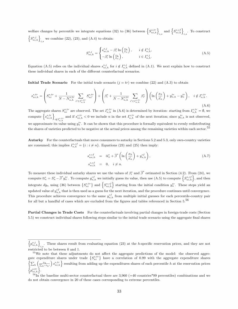
welfare changes by percentile we integrate equations (32) to (36) betweenSs,trni,h

i,s

andSs,cfni,h

i,s

. To constructSs,jni,h

i,s

we combine (22), (23), and (A.4) to obtain:

Ss,jni,h =

ss,jni,h − β

si ln

(xhxn

), i /∈ Is,jn,h,

−βsi ln(xhxn

), i ∈ Is,jn,h.

(A.5)

Equation (A.5) relies on the individual shares ss,jni,h for i /∈ Is,jn,h defined in (A.1). We next explain how to construct

these individual shares in each of the different counterfactual scenarios.

Initial Trade Scenario For the initial trade scenario (j = tr) we combine (22) and (A.3) to obtain

ss,trni,h =

Ss,trni +1

N −Ns,trn,h

∑i′∈Is,tr

n,h

Ss,trni′

+

βsi +1

N −Ns,trn,h

∑i′∈Is,tr

n,h

βsi′

(ln

(xhxn

)+ ytrn,h − ytrn

), i /∈ Is,trn,h .

(A.6)

The aggregate shares Ss,trni are observed. The set Is,trn,h in (A.6) is determined by iteration: starting from Is,trn,h = ∅, we

computess,trni,h

i/∈Is,tr

n,h

and if ss,trni,h < 0 we include n in the set Is,trn,h of the next iteration; since ytrn,h is not observed,

we approximate its value using ytrn . It can be shown that this procedure is formally equivalent to evenly redistributing

the shares of varieties predicted to be negative at the actual prices among the remaining varieties within each sector.55

Autarky For the counterfactuals that move consumers to autarky in Sections 5.2 and 5.3, only own-country varieties

are consumed; this implies Is,cfn,h = i : i 6= n. Equations (23) and (25) then imply:

ss,cfnn,h = αsn + βs(

ln

(xhxn

)+ ycfn,h

), (A.7)

ss,cfni,h = 0, i 6= n.

To measure these individual autarky shares we use the values of βsi and βs

estimated in Section (4.2). From (24), we

compute αsn = Ssn−βsytrn . To compute ycfn,h we initially guess its value, then use (A.5) to compute

Ss,cfni,h

, and then

integrate dyn using (36) betweenSs,trni

and

Ss,cfni,h

starting from the initial condition ytrn . These steps yield an

updated value of ycfn,h that is then used as a guess for the next iteration, and the procedure continues until convergence.

This procedure achieves convergence to the same ycfn,h from multiple initial guesses for each percentile-country pair

for all but a handful of cases which are excluded from the figures and tables referenced in Section 5.56

Partial Changes in Trade Costs For the counterfactuals involving partial changes in foreign-trade costs (Section

5.5) we construct individual shares following steps similar to the initial trade scenario using the aggregate final shares

ps,jni,h

i,s

. These shares result from evaluating equation (23) at the h-specific reservation prices, and they are not

restricted to be between 0 and 1.55We note that these adjustments do not affect the aggregate predictions of the model: the observed aggre-

gate expenditure shares under tradeSs,trni

have a correlation of 0.99 with the aggregate expenditure shares∑

h

(xh∑h′ xh′

)ss,trni,h

resulting from adding up the expenditures shares of each percentile h at the reservation prices

ps,trni,h

.

56In the baseline multi-sector counterfactual there are 3,960 (=40 countries*99 percentiles) combinations and wedo not obtain convergence in 20 of these cases corresponding to extreme percentiles.

33

Ss,cfin = Ss,trin + ∆Ssni. The term ∆Ssni can be computed from (22), which implies

∆Ssni = −γs[

∆ ln τsni −1

N

N∑i′=1

∆ ln τsni′

]+ βsi∆yn. (A.8)

We integrate dyn = −∑s

∑i (Ssni − βsi yn) τsni (which follows from Shepard’s Lemma) and dSsni = −γs

[ˆτsni − 1

N

∑Ni′=1

ˆτsni′]+

βsi dyn (which follows from (A.8)) to obtain ∆yn.

B Computing Welfare Changes with a Non-Traded Sector

We derive the welfare results assuming that a subset of sectors are non-traded. Assume that s = NT is a non-

traded sector. We show that equations (32) to (36) for the welfare effects of a foreign-trade shock remain the same

with the only difference being that the non-traded sector is excluded from the expressions.

In sector s = NT , the preferences of country n are only defined over the variety produced by country n. We

let βNT be the income elasticity corresponding to the non-traded sector. The adding-up constrain then implies

γNT = 0, βNT = −∑s6=NT

∑Ni=1 β

si , and αNTnn = αNTn = 1 −

∑s6=NT α

sn. Letting SNTn be the share of expenditures

in non-traded goods, the aggregate expenditure shares (22) in country n are now defined as follows:

Ssni = αsni − γs[

ln

(psniˆpsnn

)− 1

N

N∑i′=1

ln

(psni′

ˆpsnn

)]+ βsi yn for s 6= NT , (A.9)

SNTn = αNTn + βNT yn. (A.10)

In changes, equation (A.9) can be written as:

psni − psnn = −dSsni − dSsnnγs

+1

γs(βsi − βsn) dyn. (A.11)

Additionally, we have that:

psnn = pNTnn = wn. (A.12)

Since xh = wn, the welfare change of consumer h defined in (4) is:

ωh = Wn − bn × ln(xhx

)+ wn. (A.13)

where, using (5) and (13), we have

Wn =∑s6=NT

∑i

(−psni)Ssni − pNTnn SNTn , (A.14)

bn =∑s6=NT

∑i

psniβsi + pNTnn β

NT . (A.15)

Combining (A.11) to (A.15), and using the normalization of the own wage (wn = 0), leads to:

Wn =∑s6=NT

∑i

(dSsni − dSsnn + (βsn − βsi ) dyn)Ssniγs

,

bn =∑s6=NT

∑i

βsiγs

(dSsnn − dSsni + (βsi − βsn) dyn) ,

which correspond to (32) to (35) when all sectors are traded. To characterize welfare changes it remains to solve for

34

dy. From Shephard’s Lemma,

an ≡∑s6=NT

∑i

∂ ln a

∂ ln psnipsni +

∂ ln a

∂ ln pNTnpNTn ,

=∑s6=NT

∑i

(Ssni − βsniyn) psni +(SNTn − βNTn yn

)pNTn .

Combining this expression with (A.11) to (A.15), using that dyn = wn − an and solving for dyn yields

dyn =

∑s6=NT

∑i

1γs

(Ssni − βsniyn) (dSsni − dSsnn)

1−∑s6=NT

∑i

1γs

(Ssni − βsi yn) (βsn − βsi ),

which corresponds to (36) when all sectors are traded.

35

Tables and FiguresTable 1: Gravity Estimates: Single Sector

Variables (1A) (1B)-­‐Distanceni 0.043 ***

(0.005)

Languageni 0.131 ***(0.021)

Borderni 0.135 ***(0.023)

Ωn X Ωn X

β-­‐USA 0.052 ** β-­‐POL -­‐0.001(0.022) (0.011)

β-­‐JPN 0.028 *** β-­‐IDN -­‐0.023(0.008) (0.032)

β-­‐CHN 0.008 β-­‐AUT -­‐0.001(0.031) (0.009)

β-­‐DEU -­‐0.015 β-­‐DNK 0.003(0.013) (0.009)

β-­‐GBR 0.005 β-­‐GRC 0.018 *(0.013) (0.009)

β-­‐FRA -­‐0.013 β-­‐IRL -­‐0.009(0.011) (0.013)

β-­‐ITA 0.006 β-­‐FIN 0.013(0.006) (0.010)

β-­‐ESP -­‐0.004 β-­‐PRT -­‐0.001(0.006) (0.005)

β-­‐CAN -­‐0.017 β-­‐CZE -­‐0.003(0.015) (0.006)

β-­‐KOR 0.006 β-­‐ROM 0.003(0.012) (0.015)

β-­‐IND -­‐0.048 β-­‐HUN 0.008(0.042) (0.012)

β-­‐BRA -­‐0.010 β-­‐SVK 0.005(0.017) (0.010)

β-­‐RUS -­‐0.003 β-­‐LUX -­‐0.012 *(0.022) (0.007)

β-­‐MEX -­‐0.029 * β-­‐SVN -­‐0.002(0.017) (0.005)

β-­‐AUS 0.011 β-­‐BGR 0.004(0.012) (0.016)

β-­‐NLD -­‐0.008 β-­‐LTU 0.004(0.009) (0.010)

β-­‐TUR 0.006 β-­‐LVA 0.006(0.016) (0.009)

β-­‐BEL -­‐0.025 ** β-­‐EST 0.007(0.011) (0.007)

β-­‐TWN 0.017 β-­‐CYP 0.016 **(0.011) (0.008)

β-­‐SWE 0.006 β-­‐MLT -­‐0.006(0.008) (0.010)

Joint F-­‐test p-­‐value for income elasticities 0.00R2 0.47Observations 1,600Implied γ 0.24Notes: Table reports the estimates of the single-­‐sector gravity equation that aggregates the dataacross the 35 sectors. There are 40 income elasticity parameters βi. We assume that ρ=0.177,

and the implied γ=coefficient on -­‐Distanceni/ρ is noted at the bottom of the table. Standarderrors are clustered by importer. Significance * .10; ** .05; *** .01.

Table 2: Engel Curve Estimation: Baseline

Variables (1A) (1B)Agriculture -­‐0.0218 *** Electricity, Gas and Water Supply -­‐0.0033

(0.002) (0.002)

Mining -­‐0.0080 *** Construction -­‐0.0053(0.002) (0.003)

Food, Beverages and Tobacco -­‐0.0125 *** Sale, Repair of Motor Vehicles 0.0027 ***(0.003) (0.001)

Textiles -­‐0.0063 *** Wholesale Trade and Commission Trade 0.0010(0.001) (0.003)

Leather and Footwear -­‐0.0009 *** Retail Trade -­‐0.0020(0.000) (0.002)

Wood Products -­‐0.0008 Hotels and Restaurants 0.0021(0.001) (0.001)

Printing and Publishing 0.0014 * Inland Transport -­‐0.0089 ***(0.001) (0.003)

Coke, Refined Petroleum, Nuclear Fuel -­‐0.0056 *** Water Transport -­‐0.0007(0.002) (0.001)

Chemicals and Chemical Products -­‐0.0046 *** Air Transport 0.0007 *(0.001) (0.000)

Rubber and Plastics -­‐0.0016 * Other Auxiliary Transport Activities 0.0038 ***(0.001) (0.001)

Other Non-­‐Metallic Minerals -­‐0.0027 *** Post and Telecommunications 0.0012(0.001) (0.001)

Basic Metals and Fabricated Metal -­‐0.0031 Financial Intermediation 0.0280(0.004) (0.018)

Machinery -­‐0.0028 Real Estate Activities 0.0095 ***(0.002) (0.003)

Electrical and Optical Equipment -­‐0.0021 Renting of M&Eq 0.0243 ***(0.003) (0.003)

Transport Equipment -­‐0.0033 * Public Admin and Defence 0.0038(0.002) (0.003)

Manufacturing, nec -­‐0.0005 Education 0.0022 **(0.001) (0.001)

Health and Social Work 0.0128 ***(0.003)

Other Community and Social Services 0.0031(0.003)

Private Households with Employed Persons 0.0003 **(0.000)

Sector FEs yesJoint F-­‐test p-­‐value for sectoral elasticities 0.00R-­‐squared 0.67Observations 1,400Notes: Table reports the sectoral income elasticities from the Engel curve equation. It is a regression of importers' sectoral expendituresshares on the adjusted real income interacted with sector dummies. Sectors "Agriculture" and "Food, Beverages and Tobacco" are thefood sectors, and the remaining sectors in column 1A are the manufacturing sectors; the service sectors are listed in column 1B. Theregression also includes sector fixed effects. Standard errors are clustered by importer. Significance * .10; ** .05; *** .01.

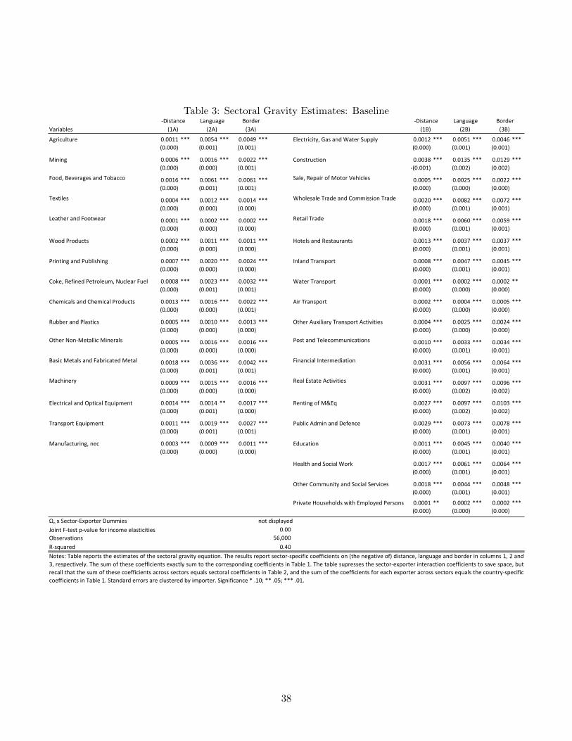
Table 3: Sectoral Gravity Estimates: Baseline

Variables (1A) (2A) (3A) (1B) (2B) (3B)

Agriculture 0.0011 *** 0.0054 *** 0.0049 *** Electricity, Gas and Water Supply 0.0012 *** 0.0051 *** 0.0046 ***(0.000) (0.001) (0.001) (0.000) (0.001) (0.001)

Mining 0.0006 *** 0.0016 *** 0.0022 *** Construction 0.0038 *** 0.0135 *** 0.0129 ***(0.000) (0.000) (0.001) -­‐(0.001) (0.002) (0.002)

Food, Beverages and Tobacco 0.0016 *** 0.0061 *** 0.0061 *** Sale, Repair of Motor Vehicles 0.0005 *** 0.0025 *** 0.0022 ***(0.000) (0.001) (0.001) (0.000) (0.000) (0.000)

Textiles 0.0004 *** 0.0012 *** 0.0014 *** Wholesale Trade and Commission Trade 0.0020 *** 0.0082 *** 0.0072 ***(0.000) (0.000) (0.000) (0.000) (0.001) (0.001)

Leather and Footwear 0.0001 *** 0.0002 *** 0.0002 *** Retail Trade 0.0018 *** 0.0060 *** 0.0059 ***(0.000) (0.000) (0.000) (0.000) (0.001) (0.001)

Wood Products 0.0002 *** 0.0011 *** 0.0011 *** Hotels and Restaurants 0.0013 *** 0.0037 *** 0.0037 ***(0.000) (0.000) (0.000) (0.000) (0.001) (0.001)

Printing and Publishing 0.0007 *** 0.0020 *** 0.0024 *** Inland Transport 0.0008 *** 0.0047 *** 0.0045 ***(0.000) (0.000) (0.000) (0.000) (0.001) (0.001)

Coke, Refined Petroleum, Nuclear Fuel 0.0008 *** 0.0023 *** 0.0032 *** Water Transport 0.0001 *** 0.0002 *** 0.0002 **(0.000) (0.001) (0.001) (0.000) (0.000) (0.000)

Chemicals and Chemical Products 0.0013 *** 0.0016 *** 0.0022 *** Air Transport 0.0002 *** 0.0004 *** 0.0005 ***(0.000) (0.000) (0.001) (0.000) (0.000) (0.000)

Rubber and Plastics 0.0005 *** 0.0010 *** 0.0013 *** Other Auxiliary Transport Activities 0.0004 *** 0.0025 *** 0.0024 ***(0.000) (0.000) (0.000) (0.000) (0.000) (0.000)

Other Non-­‐Metallic Minerals 0.0005 *** 0.0016 *** 0.0016 *** Post and Telecommunications 0.0010 *** 0.0033 *** 0.0034 ***(0.000) (0.000) (0.000) (0.000) (0.001) (0.001)

Basic Metals and Fabricated Metal 0.0018 *** 0.0036 *** 0.0042 *** Financial Intermediation 0.0031 *** 0.0056 *** 0.0064 ***(0.000) (0.001) (0.001) (0.000) (0.001) (0.001)

Machinery 0.0009 *** 0.0015 *** 0.0016 *** Real Estate Activities 0.0031 *** 0.0097 *** 0.0096 ***(0.000) (0.000) (0.000) (0.000) (0.002) (0.002)

Electrical and Optical Equipment 0.0014 *** 0.0014 ** 0.0017 *** Renting of M&Eq 0.0027 *** 0.0097 *** 0.0103 ***(0.000) (0.001) (0.000) (0.000) (0.002) (0.002)

Transport Equipment 0.0011 *** 0.0019 *** 0.0027 *** Public Admin and Defence 0.0029 *** 0.0073 *** 0.0078 ***(0.000) (0.001) (0.001) (0.000) (0.001) (0.001)

Manufacturing, nec 0.0003 *** 0.0009 *** 0.0011 *** Education 0.0011 *** 0.0045 *** 0.0040 ***(0.000) (0.000) (0.000) (0.000) (0.001) (0.001)

Health and Social Work 0.0017 *** 0.0061 *** 0.0064 ***(0.000) (0.001) (0.001)

Other Community and Social Services 0.0018 *** 0.0044 *** 0.0048 ***(0.000) (0.001) (0.001)

Private Households with Employed Persons 0.0001 ** 0.0002 *** 0.0002 ***(0.000) (0.000) (0.000)

Ωn x Sector-­‐Exporter Dummies not displayedJoint F-­‐test p-­‐value for income elasticities 0.00Observations 56,000R-­‐squared 0.40

Language Border

Notes: Table reports the estimates of the sectoral gravity equation. The results report sector-­‐specific coefficients on (the negative of) distance, language and border in columns 1, 2 and3, respectively. The sum of these coefficients exactly sum to the corresponding coefficients in Table 1. The table supresses the sector-­‐exporter interaction coefficients to save space, butrecall that the sum of these coefficients across sectors equals sectoral coefficients in Table 2, and the sum of the coefficients for each exporter across sectors equals the country-­‐specificcoefficients in Table 1. Standard errors are clustered by importer. Significance * .10; ** .05; *** .01.

-­‐Distance Language Border -­‐Distance

38

Table 4: Aggregate Gains from Trade: AIDS vs Translog

CountryAggregate Gains

(AIDS)Aggregate Gains

(Translog)Gains at Median

(AIDS)Country Import

Share CountryAggregate Gains

(AIDS)Aggregate Gains

(Translog)Gains at Median

(AIDS)Country Import

Share(1A) (2A) (3A) (4A) (1B) (2B) (3B) (4B)

AUS 9% 8% 24% 8% IRL 40% 43% 52% 32%AUT 42% 41% 56% 23% ITA 13% 12% 31% 10%BEL 50% 51% 63% 28% JPN 6% 5% 24% 5%BGR 46% 45% 58% 25% KOR 16% 16% 33% 11%BRA 2% 2% 20% 4% LTU 67% 64% 77% 27%CAN 29% 30% 44% 16% LUX 86% 85% 89% 49%CHN 6% 7% 16% 7% LVA 36% 35% 52% 22%CYP 43% 40% 57% 22% MEX 24% 24% 40% 14%CZE 50% 49% 60% 26% MLT 66% 66% 75% 34%DEU 26% 26% 40% 17% NLD 28% 28% 45% 21%DNK 41% 40% 54% 22% POL 27% 26% 42% 18%ESP 17% 16% 34% 12% PRT 27% 26% 46% 17%EST 50% 48% 65% 27% ROM 34% 33% 49% 19%FIN 28% 26% 46% 17% RUS 16% 16% 32% 9%FRA 15% 15% 29% 12% SVK 67% 64% 74% 30%GBR 14% 13% 33% 12% SVN 55% 54% 66% 27%GRC 26% 24% 44% 15% SWE 29% 27% 43% 19%HUN 68% 67% 76% 31% TUR 11% 11% 29% 10%IDN 5% 5% 11% 8% TWN 41% 41% 56% 20%IND 6% 6% 10% 6% USA 8% 6% 37% 6%Average 32% 31% 46% 18%Notes: Table reports gains from trade. The first and third columns repors the gains for the representative agent and median consumer, respectively, using the estimatedparameters from Tables 2 and 3. The second column computes welfare changes using a translog demand system; these parameters are obtained from re-­‐running the

gravity equation imposing βsi=0 (see Appendix Table A.1). The fourth column reports the aggregate import share for each country.

Table 5: Unequal Gains From Trade: Baseline

Country10th

percentile50th

PercentileAggregate Gains

90th Percentile Country

10th percentile

50th Percentile

Aggregate Gains

90th Percentile

(1A) (2A) (3A) (4A) (1B) (2B) (3B) (4B)AUS 45% 24% 9% 5% IRL 67% 52% 40% 38%AUT 68% 56% 42% 38% ITA 52% 31% 13% 8%BEL 75% 63% 50% 46% JPN 46% 24% 6% 2%BGR 72% 58% 46% 43% KOR 53% 33% 16% 12%BRA 57% 20% 2% 3% LTU 87% 77% 67% 63%CAN 60% 44% 29% 25% LUX 91% 89% 86% 85%CHN 38% 16% 6% 6% LVA 70% 52% 36% 32%CYP 71% 57% 43% 39% MEX 65% 40% 24% 21%CZE 71% 60% 50% 47% MLT 83% 75% 66% 64%DEU 56% 40% 26% 21% NLD 61% 45% 28% 24%DNK 67% 54% 41% 37% POL 61% 42% 27% 23%ESP 53% 34% 17% 12% PRT 67% 46% 27% 22%EST 79% 65% 50% 46% ROM 67% 49% 34% 31%FIN 64% 46% 28% 23% RUS 56% 32% 16% 14%FRA 45% 29% 15% 11% SVK 82% 74% 67% 64%GBR 54% 33% 14% 10% SVN 76% 66% 55% 52%GRC 63% 44% 26% 21% SWE 59% 43% 29% 25%HUN 84% 76% 68% 65% TUR 56% 29% 11% 8%IDN 24% 11% 5% 4% TWN 72% 56% 41% 37%IND 19% 10% 6% 6% USA 69% 37% 8% 4%Average 63% 46% 32% 28%Notes: Table reports gains from trade for the baseline multi-­‐sector model and uses the parameters reported in Tables 2 and 3. The columnsreport welfare changes associated at the 10th, 50th, the representative consumer (taken from column 1 of Table 4), and the 90thpercentiles.

39

Figure 1: βi and GDPPC

USA

JPN

CHN

DEU

GBR

FRA

ITA

ESP

CAN

KOR

IND

BRA

RUS

MEX

AUS

NLD

TUR

BEL

TWN

SWE

POL

IDN

AUTDNK

GRC

IRL

FIN

PRTCZE

ROM

HUNSVK

LUX

SVN

BGR LTULVA EST

CYP

MLT

−.0

50

.05

βi

8 9 10 11 12Log GDP per Capita

Figure plots exporter income elasticity against its per capita GDP

Figure 2: Engel Curves, by Broad Sector Groups

0.2

.4.6

.8S

ha

re o

f A

gg

reg

ate

Exp

en

ditu

res

8 9 10 11 12Log GDP per Capita

Food Mfg Services

Figure displays Engel curves of expenditure shares in broad sectors against per capita GDP.See the note in Table 2 for the list of sectors.

40

Figure 3: β by Exporter and Broad Sector Group vs GDPPC

−.0

20

.02

.04

Beta

8 9 10 11 12Log GDP per Capita

Food Mfg Services

Figure plots income elasticities, summed across broad sectors for each country, against per capita GDP.See the note in Table 2 for the list of sectors.

Figure 4: Distribution of Unequal Gains: Single-Sector Case

DEU

FINJPN

SVK

ROM

ESP

IRL

LTU

HUN

USA

IDN

BEL

GBR

ITA

MLT

TWN

SVN

DNK

CAN

CZE

IND

BGR

POL

CYP

TUR

FRA

SWE

GRC

MEX

CHN

PRT

NLD

LUX

AUTKOR

LVA

AUS

EST

RUSBRA

POL

GBR

SWE

TUR

LTU

INDIRL

LVATWN

ESP

AUS

BRA

CAN

ROM

SVN

RUS

LUX

MEX

EST

KORITA

AUT

CYP

PRT

FRAMLT

NLD

GRC

IDN

CHN

SVK

CZE

DEU

JPN

BGR

HUN

DNK

USA

BEL

FIN

−.0

50

.05

.1.1

5G

ain

s fro

m T

rade R

ela

tive to M

edia

n

0 .1 .2 .3 .4 .5 .6 .7 .8 .9 1Income Percentile

The deviations are relative to the median individual. The red line is the average across countries.

41

Figure 5: Distribution of Unequal Gains: Baseline Case

SWE

HUN

BRA

PRT

IRLNLD

AUT

FRA

BEL IND

GBR

CHN

KOR

CZE

CYP

CAN

DNK

MLT

TWN

IDN

MEX

LUX

RUS

SVK

AUS

FIN

EST

GRC

USA

SVN

LVA

ESP

ITA

LTU

DEU

TUR

JPN

ROM

BGR

POL

CYP

IND

EST

IRL

TWN

ESP

FIN

ROM

CHN

NLD

AUS

FRA

AUT

ITA

PRT

HUN

POL

DEU

JPN

BEL

KOR

GRC

LVA

LUX

SVN

SWE

CAN

IDN

CZE

LTU

BGR

SVKMLT

DNK

−.4

−.2

0.2

.4.6

Gain

s fro

m T

rade R

ela

tive to M

edia

n

0 .1 .2 .3 .4 .5 .6 .7 .8 .9 1Income Percentile

The deviations are relative to the median individual. The red line is the average across countries.

Figure 6: Comparison of Distribution of Unequal Gains, Means across Countries

−.4

−.2

0.2

.4G

ain

s f

rom

Tra

de

, R

ela

tive

to

Me

dia

n

0 .1 .2 .3 .4 .5 .6 .7 .8 .9 1Income Percentile

1 Single−Sector 2 Multi−Sector, Homothetic, Asymmetric−γ

3 Multi−Sector, Non−Homothetic, Symmetric−γ 4 Multi−Sector (Baseline)

The deviations are relative to the median individual. Figure shows averages across countries, by percentile.

42

Figure 7: Difference in Gains From Trade Between 90th and 10th Percentiles vs βi

AUS

AUTBEL BGR

BRA

CANCHN CYP

CZE

DEU

DNK

ESP

EST

FIN

FRA

GBRGRC

HUNIDN

IND

IRL

ITA JPN

KOR

LTU

LUX

LVA

MEX

MLT

NLD POL

PRT

ROM

RUS

SVK

SVN

SWE

TUR

TWN

USA

−.6

−.4

−.2

090−

10 W

elfare

Diffe

rence

−.05 0 .05(βi)

Figure plots the difference in gains from trade between 90th and 10th percentiles againstthe country’s income elasticity

Figure 8: Varying Sectoral Income Elasticities

−.4

−.2

0.2

.4G

ain

s fro

m T

rade, R

ela

tive to M

edia

n

0 .1 .2 .3 .4 .5 .6 .7 .8 .9 1Income Percentile

Baseline

Engel Curves from Within Variation

Engel Curves from CE Data

The deviations are relative to the median individual. Figure shows averages across countries, by percentile.

43

Figure 9: Varying Price Elasticity for Less-Traded Services

−.2

0.2

.4G

ain

s fro

m T

rade, R

ela

tive to M

edia

n

0 .1 .2 .3 .4 .5 .6 .7 .8 .9 1Income Percentile

Baseline

Increase ρ for less−traded services sectors

Remove less−traded services sectors

The deviations are relative to the median individual. Figure shows averages across countries, by percentile.

Figure 10: Varying the Value of ρ

−.4

−.2

0.2

.4G

ain

s fro

m T

rade, R

ela

tive to M

edia

n

0 .1 .2 .3 .4 .5 .6 .7 .8 .9 1Income Percentile

Baseline ρ=0.133 ρ=0.221

The deviations are relative to the median individual. Figure shows averages across countries, by percentile.

44

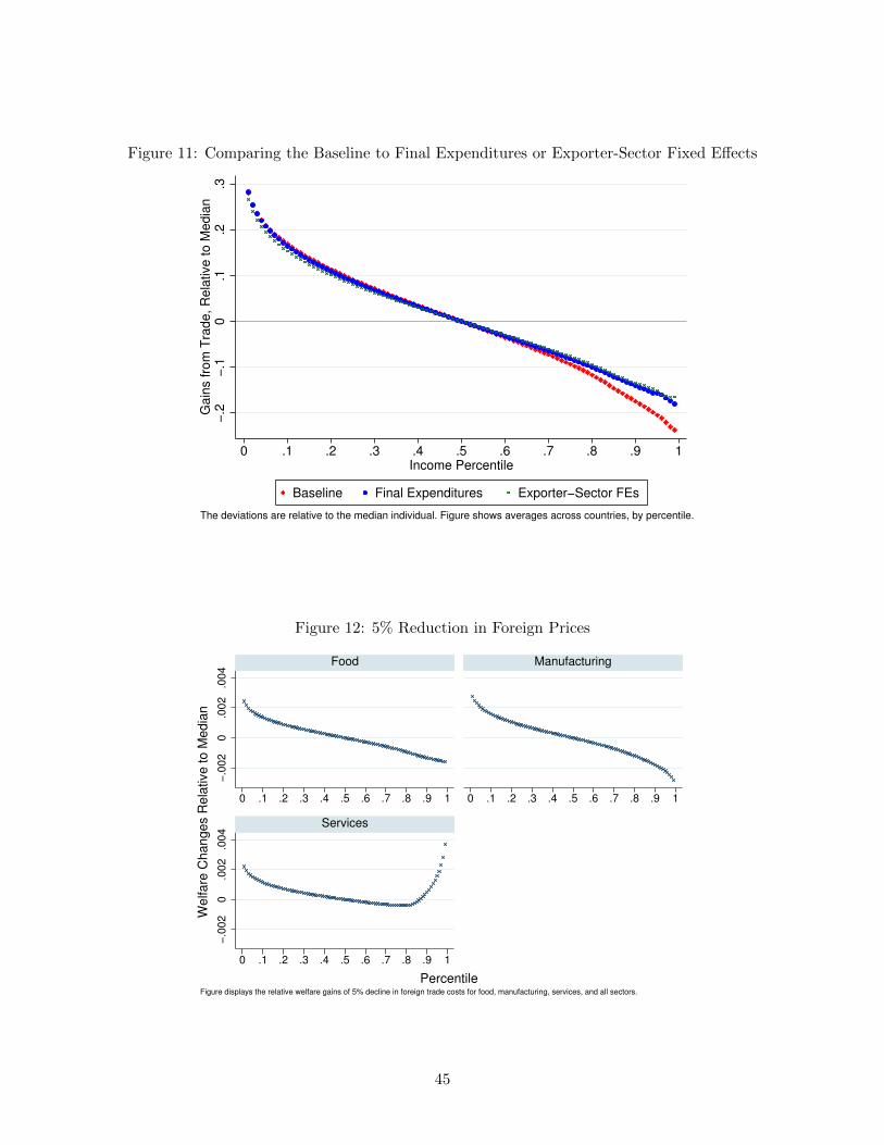
Figure 11: Comparing the Baseline to Final Expenditures or Exporter-Sector Fixed Effects

−.2

−.1

0.1

.2.3

Gain

s fro

m T

rade, R

ela

tive to M

edia

n

0 .1 .2 .3 .4 .5 .6 .7 .8 .9 1Income Percentile

Baseline Final Expenditures Exporter−Sector FEs

The deviations are relative to the median individual. Figure shows averages across countries, by percentile.

Figure 12: 5% Reduction in Foreign Prices

−.0

02

0.0

02

.00

4−

.00

20

.00

2.0

04

0 .1 .2 .3 .4 .5 .6 .7 .8 .9 1 0 .1 .2 .3 .4 .5 .6 .7 .8 .9 1

0 .1 .2 .3 .4 .5 .6 .7 .8 .9 1

Food Manufacturing

Services

Welfare

Changes R

ela

tive to M

edia

n

PercentileFigure displays the relative welfare gains of 5% decline in foreign trade costs for food, manufacturing, services, and all sectors.

45

Appendix Tables and Figures

Table A.1: Multi-Sector Translog Gravity Equation

Variables (1A) (2A) (3A) (1B) (2B) (3B)

Agriculture 0.0013 *** 0.0049 *** 0.0051 *** Electricity, Gas and Water Supply 0.0013 *** 0.0050 *** 0.0046 ***(0.000) (0.001) (0.001) (0.000) (0.001) (0.001)

Mining 0.0006 *** 0.0016 *** 0.0023 *** Construction 0.0039 *** 0.0131 *** 0.0128 ***(0.000) (0.000) (0.001) -­‐(0.001) (0.002) (0.002)

Food, Beverages and Tobacco 0.0017 *** 0.0059 *** 0.0061 *** Sale, Repair of Motor Vehicles 0.0005 *** 0.0024 *** 0.0021 ***(0.000) (0.001) (0.001) (0.000) (0.000) (0.000)

Textiles 0.0004 *** 0.0011 *** 0.0014 *** Wholesale Trade and Commission Trade 0.0020 *** 0.0081 *** 0.0071 ***(0.000) (0.000) (0.000) (0.000) (0.001) (0.001)

Leather and Footwear 0.0001 *** 0.0002 *** 0.0002 *** Retail Trade 0.0018 *** 0.0059 *** 0.0060 ***(0.000) (0.000) (0.000) (0.000) (0.001) (0.001)

Wood Products 0.0002 *** 0.0011 *** 0.0011 *** Hotels and Restaurants 0.0013 *** 0.0037 *** 0.0037 ***(0.000) (0.000) (0.000) (0.000) (0.001) (0.001)

Printing and Publishing 0.0006 *** 0.0020 *** 0.0024 *** Inland Transport 0.0009 *** 0.0044 *** 0.0045 ***(0.000) (0.000) (0.000) (0.000) (0.001) (0.001)

Coke, Refined Petroleum, Nuclear Fuel 0.0008 *** 0.0021 *** 0.0033 *** Water Transport 0.0001 *** 0.0002 *** 0.0002 ***(0.000) (0.001) (0.001) (0.000) (0.000) (0.000)

Chemicals and Chemical Products 0.0013 *** 0.0016 *** 0.0023 *** Air Transport 0.0002 *** 0.0004 *** 0.0005 ***(0.000) (0.000) (0.001) (0.000) (0.000) (0.000)

Rubber and Plastics 0.0005 *** 0.0010 *** 0.0013 *** Other Auxiliary Transport Activities 0.0004 *** 0.0024 *** 0.0023 ***(0.000) (0.000) (0.000) (0.000) (0.000) (0.000)

Other Non-­‐Metallic Minerals 0.0005 *** 0.0015 *** 0.0016 *** Post and Telecommunications 0.0010 *** 0.0033 *** 0.0033 ***(0.000) (0.000) (0.000) (0.000) (0.001) (0.001)

Basic Metals and Fabricated Metal 0.0017 *** 0.0034 *** 0.0045 *** Financial Intermediation 0.0031 *** 0.0056 *** 0.0064 ***(0.000) (0.001) (0.001) -­‐(0.001) (0.001) (0.001)

Machinery 0.0008 *** 0.0014 *** 0.0017 *** Real Estate Activities 0.0029 *** 0.0097 *** 0.0095 ***(0.000) (0.000) (0.000) (0.000) (0.002) (0.002)

Electrical and Optical Equipment 0.0014 *** 0.0013 *** 0.0018 *** Renting of M&Eq 0.0026 *** 0.0097 *** 0.0102 ***(0.000) (0.001) (0.000) (0.000) (0.002) (0.002)

Transport Equipment 0.0011 *** 0.0018 *** 0.0028 *** Public Admin and Defence 0.0027 *** 0.0074 *** 0.0078 ***(0.000) (0.001) (0.001) (0.000) (0.001) (0.001)

Manufacturing, nec 0.0003 *** 0.0009 *** 0.0011 *** Education 0.0012 *** 0.0044 *** 0.0039 ***(0.000) (0.000) (0.000) (0.000) (0.001) (0.001)

Health and Social Work 0.0016 *** 0.0061 *** 0.0063 ***(0.000) (0.001) (0.001)

Other Community and Social Services 0.0017 *** 0.0045 *** 0.0047 ***(0.000) (0.001) (0.001)

Private Households with Employed Persons 0.0001 *** 0.0002 *** 0.0002 ***(0.000) (0.000) (0.000)

R-­‐squared 0.38Observations 56,000

-­‐Distance Language Border -­‐Distance Language Border

Notes: Table reports the estimates of the multi-­‐sector translog gravity equation, which shuts of non-­‐homotheticities. The results report sector-­‐specific coefficients on (thenegative of) distance, language and border in columns 1, 2 and 3, respectively. Standard errors are clustered by importer. Significance * .10; ** .05; *** .01.

46

Table A.2: Engel Curve Estimates: Final ExpendituresVariables (1A) (1B)Agriculture -­‐0.0219 *** Electricity, Gas and Water Supply 0.0005

(0.003) (0.001)

Mining -­‐0.0005 Construction -­‐0.0169 **(0.000) (0.008)

Food, Beverages and Tobacco -­‐0.0169 *** Sale, Repair of Motor Vehicles 0.0037 ***(0.004) (0.001)

Textiles -­‐0.0045 *** Wholesale Trade and Commission Trade 0.0009(0.001) (0.003)

Leather and Footwear -­‐0.0009 *** Retail Trade 0.0012(0.000) (0.002)

Wood Products 0.0002 Hotels and Restaurants 0.0056 **(0.000) (0.002)

Printing and Publishing 0.0021 *** Inland Transport -­‐0.0083 ***(0.000) (0.003)

Coke, Refined Petroleum, Nuclear Fuel -­‐0.0004 Water Transport -­‐0.0010(0.001) (0.001)

Chemicals and Chemical Products -­‐0.0013 Air Transport 0.0005(0.001) (0.000)

Rubber and Plastics -­‐0.0003 Other Auxiliary Transport Activities 0.0017 **(0.000) (0.001)

Other Non-­‐Metallic Minerals -­‐0.0001 Post and Telecommunications 0.0003(0.000) (0.001)

Basic Metals and Fabricated Metal -­‐0.0004 Financial Intermediation 0.0061 ***(0.001) (0.002)

Machinery -­‐0.0051 * Real Estate Activities 0.0160 ***(0.003) (0.004)

Electrical and Optical Equipment -­‐0.0040 *** Renting of M&Eq 0.0039 **(0.001) (0.002)

Transport Equipment -­‐0.0031 Public Admin and Defence 0.0082 **(0.002) (0.003)

Manufacturing, nec 0.0004 Education 0.0044 ***(0.001) (0.002)

Health and Social Work 0.0246 ***(0.004)

Other Community and Social Services 0.0046(0.003)

Private Households with Employed Persons 0.0008 ***(0.000)

Sector FEs yesJoint F-­‐test p-­‐value for sectoral elasticities 0.00R-­‐squared 0.84Observations 1,400Notes: Table reports the sectoral income elasticities from the Engel curve equation using data on final expenditures. It is a regression ofimporters' sectoral expenditures shares on the adjusted real income interacted with sector dummies. The regression also includes sectorfixed effects. Standard errors are clustered by importer. Significance * .10; ** .05; *** .01.

47

Table A.3: Sectoral Gravity Estimates: Final Expenditures

Variables (1A) (2A) (3A) (1B) (2B) (3B)

Agriculture 0.0009 *** 0.0044 *** 0.0037 *** Electricity, Gas and Water Supply 0.0007 *** 0.0032 *** 0.0030 ***(0.000) (0.001) (0.001) (0.000) (0.001) (0.000)

Mining 0.0001 *** 0.0004 ** 0.0005 *** Construction 0.0065 *** 0.0190 *** 0.0182 ***(0.000) (0.000) (0.000) -­‐(0.001) (0.003) (0.004)

Food, Beverages and Tobacco 0.0020 *** 0.0071 *** 0.0077 *** Sale, Repair of Motor Vehicles 0.0005 *** 0.0023 *** 0.0022 ***(0.000) (0.001) (0.001) (0.000) (0.000) (0.000)

Textiles 0.0003 *** 0.0011 *** 0.0015 *** Wholesale Trade and Commission Trade 0.0021 *** 0.0070 *** 0.0062 ***(0.000) (0.000) (0.000) (0.000) (0.001) (0.001)

Leather and Footwear 0.0001 *** 0.0002 *** 0.0003 *** Retail Trade 0.0023 *** 0.0060 *** 0.0059 ***(0.000) (0.000) (0.000) (0.000) (0.001) (0.001)

Wood Products 0.0001 *** 0.0003 *** 0.0003 *** Hotels and Restaurants 0.0019 *** 0.0056 *** 0.0060 ***(0.000) (0.000) (0.000) (0.000) (0.001) (0.001)

Printing and Publishing 0.0003 *** 0.0009 *** 0.0013 *** Inland Transport 0.0007 *** 0.0036 *** 0.0031 ***(0.000) (0.000) (0.000) (0.000) (0.001) (0.001)

Coke, Refined Petroleum, Nuclear Fuel 0.0004 *** 0.0014 *** 0.0023 *** Water Transport 0.0000 *** 0.0002 *** 0.0002 ***(0.000) (0.000) (0.000) (0.000) (0.000) (0.000)

Chemicals and Chemical Products 0.0004 *** 0.0010 *** 0.0014 *** Air Transport 0.0002 *** 0.0004 *** 0.0004 ***(0.000) (0.000) (0.000) (0.000) (0.000) (0.000)

Rubber and Plastics 0.0001 *** 0.0003 *** 0.0004 *** Other Auxiliary Transport Activities 0.0003 *** 0.0014 *** 0.0014 ***(0.000) (0.000) (0.000) (0.000) (0.000) (0.000)

Other Non-­‐Metallic Minerals 0.0001 ** 0.0004 *** 0.0004 *** Post and Telecommunications 0.0009 *** 0.0024 *** 0.0025 ***(0.000) (0.000) (0.000) (0.000) (0.000) (0.000)

Basic Metals and Fabricated Metal 0.0004 *** 0.0013 *** 0.0011 *** Financial Intermediation 0.0018 *** 0.0049 *** 0.0051 ***(0.000) (0.000) (0.000) (0.000) (0.001) (0.001)

Machinery 0.0009 *** 0.0013 *** 0.0017 *** Real Estate Activities 0.0042 *** 0.0132 *** 0.0130 ***(0.000) (0.000) (0.000) -­‐(0.001) (0.002) (0.002)

Electrical and Optical Equipment 0.0008 *** 0.0013 *** 0.0016 *** Renting of M&Eq 0.0010 *** 0.0041 *** 0.0040 ***(0.000) (0.000) (0.000) (0.000) (0.001) (0.001)

Transport Equipment 0.0010 *** 0.0018 *** 0.0031 *** Public Admin and Defence 0.0055 *** 0.0141 *** 0.0137 ***(0.000) (0.001) (0.001) -­‐(0.001) (0.003) (0.003)

Manufacturing, nec 0.0004 *** 0.0008 *** 0.0013 *** Education 0.0023 *** 0.0079 *** 0.0075 ***(0.000) (0.000) (0.000) (0.000) (0.001) (0.001)

Health and Social Work 0.0034 *** 0.0116 *** 0.0116 ***-­‐(0.001) (0.002) (0.002)

Other Community and Social Services 0.0025 *** 0.0056 *** 0.0061 ***-­‐(0.001) (0.001) (0.001)

Private Households with Employed Persons 0.0001 ** 0.0004 *** 0.0003 ***(0.000) (0.000) (0.000)

Ωi x Sector-­‐Exporter Dummies not displayedJoint F-­‐test p-­‐value for income elasticities 0.00R-­‐squared 0.41Observations 56,000

-­‐Distance Language Border -­‐Distance Language Border

Notes: Table reports the estimates of the sectoral gravity equation using data on final expenditures. The results report sector-­‐specific coefficients on (the negative of) distance, languageand border in columns 1, 2 and 3, respectively. The table supresses the sector-­‐exporter interaction coefficients to save space, but recall that the sum of these coefficients across sectorsequals sectoral coefficients in Table A.2. Standard errors are clustered by importer. Significance * .10; ** .05; *** .01.

48

Table A.4: Sectoral Gravity Estimates: Exporter-Sector Fixed Effects

Variables (1A) (2A) (3A) (1B) (2B) (3B)

Agriculture 0.0015 *** 0.0065 *** 0.0044 *** Electricity, Gas and Water Supply 0.0017 *** 0.0062 *** 0.0041 ***(0.000) (0.001) (0.001) (0.000) (0.001) (0.001)

Mining 0.0007 *** 0.0020 *** 0.0019 *** Construction 0.0050 *** 0.0163 *** 0.0112 ***(0.000) (0.001) (0.001) -­‐(0.001) (0.003) (0.003)

Food, Beverages and Tobacco 0.0020 *** 0.0073 *** 0.0054 *** Sale, Repair of Motor Vehicles 0.0007 *** 0.0029 *** 0.0019 ***(0.000) (0.001) (0.001) (0.000) (0.001) (0.000)

Textiles 0.0004 *** 0.0015 *** 0.0012 *** Wholesale Trade and Commission Trade 0.0027 *** 0.0097 *** 0.0062 ***(0.000) (0.000) (0.000) (0.000) (0.002) (0.001)

Leather and Footwear 0.0001 *** 0.0002 *** 0.0002 *** Retail Trade 0.0023 *** 0.0071 *** 0.0049 ***(0.000) (0.000) (0.000) (0.000) (0.001) (0.001)

Wood Products 0.0003 *** 0.0013 *** 0.0010 *** Hotels and Restaurants 0.0016 *** 0.0044 *** 0.0031 ***(0.000) (0.000) (0.000) (0.000) (0.001) (0.001)

Printing and Publishing 0.0008 *** 0.0024 *** 0.0021 *** Inland Transport 0.0011 *** 0.0055 *** 0.0041 ***(0.000) (0.001) (0.000) (0.000) (0.001) (0.001)

Coke, Refined Petroleum, Nuclear Fuel 0.0010 *** 0.0028 *** 0.0027 *** Water Transport 0.0001 *** 0.0003 *** 0.0002 **(0.000) (0.001) (0.001) (0.000) (0.000) (0.000)

Chemicals and Chemical Products 0.0014 *** 0.0023 *** 0.0017 *** Air Transport 0.0003 *** 0.0005 *** 0.0004 ***(0.000) (0.001) (0.001) (0.000) (0.000) (0.000)

Rubber and Plastics 0.0005 *** 0.0013 *** 0.0011 *** Other Auxiliary Transport Activities 0.0006 *** 0.0029 *** 0.0022 ***(0.000) (0.000) (0.000) (0.000) (0.001) (0.000)

Other Non-­‐Metallic Minerals 0.0006 *** 0.0019 *** 0.0014 *** Post and Telecommunications 0.0013 *** 0.0040 *** 0.0029 ***(0.000) (0.000) (0.000) (0.000) (0.001) (0.001)

Basic Metals and Fabricated Metal 0.0021 *** 0.0046 *** 0.0037 *** Financial Intermediation 0.0035 *** 0.0072 *** 0.0049 ***(0.000) (0.001) (0.001) -­‐(0.001) (0.002) (0.002)

Machinery 0.0009 *** 0.0018 *** 0.0014 *** Real Estate Activities 0.0038 *** 0.0115 *** 0.0080 ***(0.000) (0.000) (0.000) -­‐(0.001) (0.002) (0.002)

Electrical and Optical Equipment 0.0016 *** 0.0019 *** 0.0011 ** Renting of M&Eq 0.0031 *** 0.0118 *** 0.0087 ***(0.000) (0.001) (0.000) -­‐(0.001) (0.003) (0.002)

Transport Equipment 0.0012 *** 0.0024 *** 0.0021 *** Public Admin and Defence 0.0033 *** 0.0088 *** 0.0063 ***(0.000) (0.001) (0.001) -­‐(0.001) (0.002) (0.002)

Manufacturing, nec 0.0003 *** 0.0010 *** 0.0009 *** Education 0.0017 *** 0.0054 *** 0.0036 ***(0.000) (0.000) (0.000) (0.000) (0.001) (0.001)

Health and Social Work 0.0021 *** 0.0073 *** 0.0055 ***(0.000) (0.002) (0.001)

Other Community and Social Services 0.0023 *** 0.0055 *** 0.0040 ***-­‐(0.001) (0.001) (0.001)

Private Households with Employed Persons 0.0001 ** 0.0002 *** 0.0001 **(0.000) (0.000) (0.000)

Ωi x Sector-­‐Exporter Dummies not displayedJoint F-­‐test p-­‐value for income elasticities 0.00R-­‐squared 0.45Observations 56,000

-­‐Distance Language Border -­‐Distance Language Border

Notes: Table reports the estimates of the sectoral gravity equation that includes sector-­‐exporter pair fixed effects. The results report sector-­‐specific coefficients on (the negative of)distance, language and border in columns 1, 2 and 3, respectively. The table supresses the sector-­‐exporter linteraction and level coefficients to save space, but recall that the sum of theinteraction coefficients across sectors equals sectoral coefficients in Table 2, and the sum of the coefficients for each exporter across sectors equals the country-­‐specific coefficients inTable 1. Standard errors are clustered by importer. Significance * .10; ** .05; *** .01.

49

Table A.5: Aggregate Gains from a 5% Decline in Manufacturing Trade Costs, AIDS vs CESAIDS CES AIDS CES

Country (1A) (2A) Country (1B) (2B)AUS 0.3% 0.3% IRL 0.6% 0.6%AUT 0.8% 0.8% ITA 0.4% 0.4%BEL 0.9% 0.9% JPN 0.2% 0.2%BGR 1.0% 1.0% KOR 0.4% 0.4%BRA 0.2% 0.1% LTU 1.0% 1.0%CAN 0.6% 0.6% LUX 0.4% 0.6%CHN 0.3% 0.3% LVA 0.8% 0.8%CYP 0.7% 0.7% MEX 0.6% 0.6%CZE 1.0% 1.0% MLT 0.8% 1.1%DEU 0.6% 0.6% NLD 0.6% 0.6%DNK 0.6% 0.6% POL 0.7% 0.7%ESP 0.5% 0.5% PRT 0.6% 0.6%EST 1.0% 1.0% ROM 0.8% 0.7%FIN 0.6% 0.6% RUS 0.4% 0.4%FRA 0.4% 0.4% SVK 1.2% 1.2%GBR 0.4% 0.4% SVN 1.0% 1.1%GRC 0.5% 0.5% SWE 0.6% 0.6%HUN 1.3% 1.2% TUR 0.4% 0.4%IDN 0.3% 0.2% TWN 0.8% 0.8%IND 0.3% 0.2% USA 0.3% 0.2%Notes: Table reports welfare changes in the multi-­‐sector model from a 5% decline inforeign trade costs in the manufacturing sectors. Column 1 reports the results using theAIDS demand system, and column 2 reports results from the CES demand system (e.g.,Ossa 2015). The elasticities for the CES system are taken from Ossa (2015) and matchedthe WIOD industry classification. The correlation between the two models is 0.99.

50

Figure A.1: βs versus Sectoral Income Elasticities from Caron et al. (2014)

.6.8

11.2

1.4

Secto

ral In

com

e E

lasticity, C

aro

n e

t al (2

014)

−.02 −.01 0 .01 .02 .03Baseline β

s Estimates

Food Manufacturing Services

Figure A.2: Average γ, by Percentile

.0095

.01

.0105

.011

Weig

hte

d−

Avera

ge G

am

ma

0 20 40 60 80 100Percentile

Weighted−average gamma calculated for baseline case

The figure reports γavh = 1

N

∑Ni=1

∑Ss′=1

ss′,adjn,h

∗ γs′, where s

s′,adjn,h

is the expenditure share of percentile h in country n on goods in sector s′.

51