IATSS Research 37 (2014) 98–109

Contents lists available at ScienceDirect

IATSS Research

Measuring the impact of urban policies on transportation energy savingusing a land use-transport model

Masanobu Kii a,⁎, Keigo Akimoto b, Kenji Doi c

a Faculty of Engineering, Kagawa University, 2217-20 Hayashi-cho, Takamatsu, Kagawa, Japanb Research Institute of Innovative Technology for the Earth (RITE), 9-2 Kizugawadai, Kizugawa-shi, Kyoto 619-0292, Japanc Department of Global Architecture, Graduate School of Engineering, Osaka University, 2-1 Yamadaoka, Suita, Osaka, Japan

⁎ Corresponding author at: Faculty of Engineering,Hayashi-cho, Takamatsu, Kagawa 761-0396, Japan. Tel.: +

E-mail addresses: kii@eng.kagawa-u.ac.jp (M. Kii), aki@doi@civil.eng.osaka-u.ac.jp (K. Doi).Peer review under responsibility of International Associatio

http://dx.doi.org/10.1016/j.iatssr.2014.03.0020386-1112/© 2014 International Association of Traffic an

a b s t r a c t

a r t i c l e i n f o

Available online 20 March 2014

Keywords:Smart citiesSustainabilityQuality of lifeUrban policiesLand-use transport model

Various projects all over the world are attempting to build smart cities in hopes of achieving energy-efficient andlivable communities, but most of them are aiming to fulfill their goals technologically. However, the energyefficiency and livability of a city are affected by not only these technological factors but also urban structuresthat encompass residential areas, offices, transportation networks, and other facilities. Urban policies intervenein transportation and land-use conditions and thereby change how citizens consume energy and go abouttheir daily lives as the actors in the urban system alter their behavior. This means that energy efficiency andquality of life share close ties. Assessments of urban policies thus need to consider the reactions of actors tothe intervention.This study demonstrates the applicability of a land-use transport model to the assessment of urban policies forbuilding smart communities. First, we outline a model that explicitly formulates the actors' location-relateddecisions and travel behavior. Second, we apply this model to two urban policies – road pricing and land-useregulation – to assess their long-term impact on energy saving and sustainability using the case of a simplifiedsynthetic city. Our study verifies that, under assumed conditions, the model has the capacity to assess urbanpolicies on energy use and sustainability in a consistent fashion.

Kagawa U81 87 864rite.or.jp

n of Traffic

d Safety Sc

© 2014 International Association of Traffic and Safety Sciences. Production and hosting by Elsevier Ltd.All rights reserved.

1. Introduction

Urban policies aimed at compaction and modal shift are consideredimportant measures for saving energy from the transportation sector.Cities can become more compact or public transportation-oriented byprompting the actors in the urban system to modify their behavior;changing household locations, moving company office locations, andexpanding transportation modes for a wider range of travel purposesare three examples of this mode of modified behavior. Urban policies,including the development of public facilities or infrastructure, trans-portation or land-use regulations, and taxes or subsidies, change theconditions of an urban system and induce behavioral changes amongthe actors in the system. As a result, urban policies affect energy use in

niversity, 2217-202140.(K. Akimoto),

and Safety Sciences.

iences. Production and hos

urban activities as well as the happiness or quality of life of people inthe city, which can serve as a representative index of sustainability.

Policies that decrease city residents' quality of life are not sustainablebecause they thwart the satisfaction of the needs of current or futuregenerations. When we evaluate urban policies as energy-savingmeasures, we should recognize not only their impact on energy savingbut also their effects on people's lives as indices of sustainability.

A land-use transport (LUT) model is an analytical tool for assessingthe impact of urban policies on people's activities and quality of life.This approach assumes the behavioral principles of people and firmswith regard to their location choices and travel in the urban system,analyzing the impact of policies on these urban activities. As a result, itis possible to calculate their energy consumption. In addition, it is possi-ble to link the estimated spatial distribution of populations and urbanactivities to the requirements of infrastructure investments thatconsume both energy and public budget funds. With this analyticaltool, one can estimate how policies affect people's happiness or qualityof life and influence transportation-related energy consumption levelsin light of the people's behavior.

The objective of this study is to demonstrate the applicability ofa LUT model to the assessment of energy-saving measures in urbantransportation systems. We have developed a LUT model that explicitlydescribes people's behavior in order to assess the effectiveness of urban

ting by Elsevier Ltd. All rights reserved.

99M. Kii et al. / IATSS Research 37 (2014) 98–109

policies in saving transportation-related energy use and evaluate theimpact of urban policies on urban sustainability. Using this model, weanalyze the repercussions of modal shift among passengers and urbancompaction in an assumed virtual city. In Section 2, we review urbanpolicies as mitigation measures and studies for urban modeling.Section 3 covers our LUT model, and Section 4 discusses the simulationresults for a modal shift policy and an urban compaction policy.

2. Urban policies and analytical models

2.1. Urban policies as transport-related energy-saving measures

Given the inextricable links between CO2 emissions and energyconsumption in urban transportation, policies to reduce CO2 emissionscontribute directly to energy saving in urban transportation. Here, wereview the literature pertaining to energy saving and CO2 emissionreduction in urban policy.

Some studies have shown that urban policies can have a substantialimpact in reducing CO2 emissions. The National Institute for Environ-mental Studies in Japan discussed policy measures to realize its visionof the urban lifestyle of the future and future reductions in CO2 emis-sions [1]. It concluded that by 2050, emissions could be reduced by70% from their 1990 level. Urban policies are responsible for part ofthe emission reductions in its model, which the institute analyzes toargue that it is possible to slash CO2 emissions from building, heating/cooling, and transportation [2]. The Intergovernmental Panel on ClimateChange (IPCC) compiled a wide range of mitigation measures in thefield of land use and transportation policy, including urban compactionand modal shift [3]. In order to promote mitigation through urbanpolicies, the Japanese government selected 13 “eco-model” cities toimplement policies for a low-carbon society [4]. In this program,the government helps the selected local governments achieve theiremission reduction targets through urban policies. The followingsection summarizes the features of urban compaction and modal shiftin passenger transportation from the literature.

2.1.1. Urban compactionUrban compaction is a policy that aims to reduce CO2 emissions and

energy consumption without undermining resident welfare by limitingthe urban sphere and leading to higher population density. Measuresthat support this policy include land-use regulations like zoning anddevelopment controls, strategic investments in urban infrastructure atthe city center, and property/land value tax systems that give prefer-ence to location and development at the city center.

This policy is designed to have the following positive effects:reduced total trip length, a modal shift from private cars to public ornon-motorized transportation, fewer expenses tied to infrastructureand buildings in suburbs, and improved efficiency of area heating/cooling because of higher city-center density. At the same time, thepotential negative effects of the policy include worse traffic congestion,increased land prices, increased construction costs, less residence/officespace per person, a risk of concentrated hazards from air pollution, andincreased energy consumption from building maintenance and opera-tions due to intensive vertical development.

Many studies highlight the effects of urban form on CO2 emissionsand energy consumption in commuting [5–9]. These studies provideempirical evidence of reduced CO2 emissions and energy consumptionin compact cities because of the shorter average commuting length.However, the findings hold only when the distributions of the activitiesare given. Gaigné et al. [10] explained that policies targeting higherdensity affect prices, wages, and land rents, which lead firms andhouseholds to relocate. Using a simple economic model, the authorsdemonstrated that such policies might actually increase emissions andenergy consumption under certain conditions. Their results underlinethe need to consider the indirect effects of compaction policies throughthe relocation of the actors involved.

Some cities are facing the problems of urban shrinkage due to eco-nomic decline, depopulation, and aging. Despite the shrinking environ-ments, these cities rarely develop amore compact urban form naturallyin themarket. Researchers have shown that this urban shrinkage causesproblems in land use and the oversupply and underuse of housingstocks [11–15],making urban compaction a potentially productive solu-tion in these cases. Compact cities require less infrastructure and tend tobe cost-effective [16]. Infrastructure requires a substantial amount ofenergy and monetary input that needs to factor into policy assessment[17].

2.1.2. Modal shift of passenger transportationAmodal shift policy aims to induce amodal shift from private cars to

public transportation or non-motorized transport, which can helpalleviate road congestion and reduce energy consumption and CO2

emissions. The following policy measures are considered effective: thedevelopment of a public transportation infrastructure, subsidies forpublic transportation operations, fare controls, traffic regulations andpricing schemes for private cars, fuel taxes, and parking fee controls[18].

By establishing these policies, cities hope to create social benefitsthrough improved services and reduced public transportation costs,curb CO2 emissions, and cut down on road congestion. However, thesepolicies can also lead to increased fiscal expenditures on public trans-portation and a decline in social welfare due to restrictions on orincreased costs of car usage.

Pigou [19] and Knight [20] took extensive looks at road pricing.Many studies have focused on finding socially optimum prices undervarious situations [21–24] but limited the assessment scope to withinroad networks and given little concern to the impact of policies onland use or competition among cities. Some studies have tried tocapture the impact on land use using the land-use transport modelswhich are described in the next section.

2.2. Urban models and land-use transport models

Although these two policies may reduce energy consumption andCO2 emissions from the transportation sector, they have both positiveand negative effects on social benefit. Assessments of the impact ofthese policies should thus evaluate not only reductions in CO2 emissionsbut also social sustainability. Because the path of the impact of urbanpolicies on social sustainability is too complicated to be readily intuitive,we need an analytical tool to determine the ways in which urbanpolicies might affect society.

There are various studies of urban models based on differenttheoretical frameworks, including the optimizationmodel of residentiallocation [25], the life-cycle assessment model for estimating lifetimeenvironmental burden from buildings and transportation [26], and theurban economics model for assessing the impacts of policies on thespatial patterns of economic activities and on social welfare [27]. Ofthese studies, only the urban economics models explicitly describepeople's behavior in a city and are able to quantify the social sustainabil-ity indices, including benefit based on behavioral principles.

LUTmodels, which integrate urban economicsmodels and transpor-tation behavior theory, provide a comprehensive analytical frameworkfor the assessment of urban policies (see review papers by Wegener[28] and Miyamoto et al. [29]). For example, Anas and Xu [30] devel-oped a general equilibriummodel of the urban activities of householdsand firms in a city, based on discrete choice theory, to assess urbanpolicies such as road pricing and the provision of public housing. Theauthors divided the urban space into discrete zones and used theirmodel to evaluate policy impact through two methods: first, theycompared the equilibrium states with and without the policy. Second,they examined where in each zone the equilibrium state representsthe simultaneous equilibrium of markets, including the commodity,labor, land, and transportation markets.

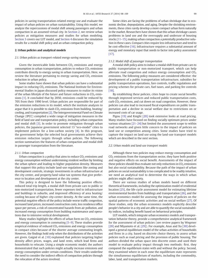
Fig. 1. Concept of vision sharing.

100 M. Kii et al. / IATSS Research 37 (2014) 98–109

2.3. Model developed for this study

The purpose of this study is to develop amethod of assessing the im-pact of urban policies on energy consumption and social sustainabilitywith a model that should be applicable to various cities with differentpopulation and economic levels. Situations and activities naturally differamong cities, especially between those in developed and less developedcountries, at least superficially. However, many cities in emergingnations are taking similar urban growth trajectories and facing thesame urban problems in land use and transportation that developedcountries have experienced. Divergent legal systems and cultures aresurely factors in shaping different urban situations, but democraticcountries can be assumed to share the essential drivers behind theformation of urban structure and activities, which are derived fromthe behavioral principles of the people or companies involved. Follow-ing the literature on LUT models, this study explains urban formationthrough the behavior of actors in the urban system under given popula-tion, technology, and productivity conditions. In our view, people andthe other actors have common behavioral principles in urban activitiesacross the world, especially with regard to the economic aspect. There-fore, we believe that ourmodel framework is applicable to various citieswhen adjusted and calibrated properly.

Technologies for smart cities would affect the urban activitiesthrough the change of costs for buildings and transportation. Buildingenergy management systems or connection of electric vehicles to thelocal power grid which are major components of smart cities is expect-ed to improve the efficiency of electric power generation. Energy ITS isanother component of smart cities which is also expected to make thetransportation more efficient. In this study, these technologies are notrepresented explicitly, but those impacts can be captured by change ofthe costs. The model is able to estimate the long term synergy andrebound effects of these technological progresses as well through thelocational shift of offices and residences. If energy technologies forbuildings reduce its costs at higher district population densities, it willenhance further energy consumption reduction over the city becausehouseholds will move to the energy efficient district reflecting thelower costs. On the other hand, if transport cost is reduced by thetechnologies, the city area is expected to expand as past LUT studiessuggested that may cancel some part of the energy consumption reduc-tion by technological progress.

As we intend to explain the impact path of policy measures, themodel is designed to output some basic indicators related to lifestyle, in-cluding income, floor area of residence, and commuting time, as socialsustainability indices. Originally LUTmodels were developed for assess-ments of the impacts of policies on urban activities, and especially ontravel behaviors. Recent LUT models based on utility theory are alsoable to estimate the policy impact on social welfare under assumptionsabout how travel patterns translate to personal well-being. Public poli-cies in the field of urban planning, transportation, energy, and environ-mental sustainability may require not only forecasts of the physicalimpact of the policies but also perspectives on the social and personalwell-being because they may bring trade-offs among policy targets.Therefore, a comprehensive assessment of wide range of impacts isneeded. Of course, a LUT model only provides partial information ofpolicy impacts on human well-being. However, if it is helpful forpolicymaking, we believe that there is a good reason to apply a LUTmodel to welfare analysis.

Ourmodel is based on past studies of LUTmodels; however, we haveupgraded some sub-models, such asfirm location and developer invest-ment behaviors, to make policy assessments more incisive. In terms ofcontributing to policy practice, we see our model as a tool that makesit easier for policymakers and relevant stakeholders to share visions ofpolicy outcomes. Fig. 1 illustrates the concept of vision sharing using aLUT model. A stakeholder in a given urban policy may have distinctiveinterests that could conflict with the interests of other stakeholders.A LUT model can be designed to analyze those different interests

consistently and visualize the outcomes spatially. The outcomes forma vision of the target urban area, a picture that stakeholders can shareto coordinate policy planning and consensus building. Past modelingstudies have largely passed over this issue and sometimes placed impactpaths in a black box. To make the analysis results accountable, we try tokeep the model as simple as possible.

3. Land-use transport model

Our model is similar in structure to the model of Anas and Xu [30],butwe include agglomeration economies in the choices for firm locationandmake the floor areas of residences and offices endogenous variablesby introducing a model of developer behavior. Some studies have takenthese factors into account [31,32], but we reformulate them within amore simplified framework. We employ the bid-rent theory [33] forthe floor market-clearing condition to reduce the computational costof the model. We also consider only passenger transportation andneglect freight transportation. Furthermore, the study restricts thescope of its transportation mode analysis to cars and trains, but thisdoes not limit its applicability to other modes.

3.1. Formulation of behaviors

We assume five classes of actors in a city: employed households,unemployed households, firms, developers, and landowners. Theprinciples of their behavior are formulated as follows.

3.1.1. The employed householdThe employed household who commutes from residential location i

to work place j determines its consumption of goods x, floor area A, andleisure hours S to maximize its utility uH under the constraints of timeand income. This behavior can be formulated as follows:

uH ¼ XijαX � AαA

ij � SijαS ð1Þ

s:t:wj � Twij þW ¼

Xk

pHik � xijk þ rij � Aij þ cij ð2Þ

T ¼ Twij þ Tc

ij þ Sij ð3Þ

where

Xij ¼X

kbk � x−ρ

ijk Þ−1ρ:

�ð4Þ

Variable k denotes the location of the shopping. Xij is the compositeutility of goods; wj is the wage rate; W is the unearned revenue; pHik is

101M. Kii et al. / IATSS Research 37 (2014) 98–109

the consumer price of goods; rij is the floor rent; cij is the commutingcost; T is the available time; Tijw is the working hours; Tijc is the commut-ing hours; and bk is the attractiveness of the shopping place. Here, theconsumer price of goods is defined as the sum of the original price ofthe goods p and the travel cost for shopping cik (pHik = p + cik). Usingthese variables, xijk, Aij, and Sij are expressed as follows:

xijk ¼ αX � wj T−Tcij

� �þW−cij

n o� bk � p−1

Hik

� � 1ρþ1

,Xk0 bk0 � p

ρHik0

� � 1ρþ1 ð5Þ

Aij ¼ αA � wj T−Tcij

� �þW−cij

n o.rij ð6Þ

Sij ¼ αS � wj T−Tcij

� �þW−cij

n o.wj: ð7Þ

For the sake of simplicity, we assume a constant return to scaleutility function.

Xα ¼ αX þ αA þ αS ¼ 1: ð8Þ

Eqs. (4) and (5) can be used to derive the following composite utilityof goods:

Xij ¼ αX � wj T−Tcij

� �þW−cij

n o.ψi ð9Þ

where ψi is a composite price of unit goods at residence i, expressed asfollows:

ψi ¼X

kbk � pρHik� � 1

ρþ1

n oρþ1ρ: ð10Þ

The indirect utility function is derived as follows:

uHij ¼ α1 � wj T−Tc

ij

� �þW−cij

n o.ψi

αX � rijαA �wjαS

� �ð11Þ

where

α1 ¼ αXαX � αA

αA � αSαS : ð12Þ

Here, under the equilibrium state, the utilities for all employedhousehold are identical, i.e. uijH ≡ uH for ∀i,j, otherwise they will moveto the higher utility pair of residence and work place. The bid rent ofthe employed household is given by following formula:

rij ¼ α1 �wj T−Tc

ij

� �þW−cij

ψiαX �wj

αS � uH

8<:

9=;

1αA

: ð13Þ

Substituting Eq. (7) into Eq. (3), working hours are given as follows:

Twij ¼ 1−αSð Þ � T−Tc

ij

� �−

αS � W−cij� �wj

: ð14Þ

The utility will be calculated endogenously to satisfy the total popu-lation constraints explained in Section 3.2. Unearned revenueW is givenexogenously assuming an outside source such as dividend from capital.

3.1.2. The unemployed householdUnemployed households consist of retired workers, who make up a

significant portion of the population in an aged society. Even thoughthey do not commute to work, they still travel for shopping purposesand thus have a significant influence on urban activities. The unem-ployed household determines its consumption of goods x and floor

area A to maximize its utility uN under the constraints of income. Thisbehavior can be described as follows.

uN ¼ XiαX � Ai

αA ð15Þ

s:t: W ¼X

kpHik � xik þ ri � Ai ð16Þ

where

Xi ¼X

kbk � x−ρ

ik Þ−1ρ:

�ð17Þ

Again we assume a constant return to scale utility function, i.e.αX + αA = 1. Solving this problem, Marshallian demands xik and Ai

are expressed as follows:

xik ¼ αX �W �bk � p−1

Hik

� � 1ρþ1

Xk0 bk0 � p

ρHik0

� � 1ρþ1

ð18Þ

Xi ¼ αX �Wψi

ð19Þ

Aij ¼ αA �Wri

: ð20Þ

The bid rent of the unemployed household is given as follows:

ri ¼α2 �Wψi

αX � uN

� � 1αA ð21Þ

α2 ¼ αXαX � αA

αA : ð22Þ

The utility for unemployed household is also calculated endoge-nously as will be explained in Section 3.2. Unearned revenue W for un-employed household is also given exogenously assuming pension fundoutside the city.

3.1.3. FirmsFirms produce goodswith inputs of labor, floor, capital, and business

meetings to maximize their profit. This is expressed as follows:

Π j ¼ p � qj−c j ð23Þ

where

qj ¼ β0 � LβLj � AβA

j � KβKj �MβM

j ð24Þ

Mj ¼Xj0

ξ � L j0 �mjj0� �−ρ

0@

1A−1

ρ

ð25Þ

c j ¼ wj � Lj þ r j � Aj þXj0

cjj0 �mjj0 þ κ � K j ð26Þ

where j is the firm location;Πj is the profit; p is the producer price; qj isthe production quantity; L, A, K, andM are the inputs of labor, floor, cap-ital, and business meetings, respectively; ξ L j′ is the value of meeting atlocation j′, which is assumed to be proportional to the labor input at j′;mjj′ is the number of meetings at j′; w is the wage rate; r is the floor

102 M. Kii et al. / IATSS Research 37 (2014) 98–109

rent; cjj′ is the travel cost between j and j′; κ is the price of capital; andβL,βA, βK, βM, and ρ are the parameters. Using these variables, Lj, Aj, Kj, andmjj′ are derived as follows:

L j ¼ p � βL � qj=wj ð27Þ

Aj ¼ p � βA � qj=r j ð28Þ

K j ¼ p � βK � qj=κ ð29Þ

mjj0 ¼ p � βM � qj �ξ � Lj0

� �−ρ

cjj0

0@

1A

1ρþ1 X

j0ξ � L j0

.cjj0

� �−ρρþ1

8<:

9=;

−1

: ð30Þ

Substituting Eq. (27)–(30) into Eq. (24) and assuming constantreturns to scale (βL + βA + βK + βM = 1), r can be solved as follows:

r j ¼p � β1ð Þ 1

βA

wj

βLβA � κ

βKβA �

Xj0

cjj0.

ξ � L j0� �� � ρ

ρþ1Þρþ1ρ �βMβA

0@

ð31Þ

where

β1 ¼ β0 � βLβL � βA

βA � βKβK � βM

βM : ð32Þ

3.1.4. DevelopersDevelopers producefloor area Aiwith inputs of landGi and construc-

tion capital Ki and provide it to firms and households to maximize theirprofit Πi. This behavior is expressed as follows:

Πi ¼ ri � Ai−φ � Ki−gi � Gi ð33Þ

Ai ¼ γ0 � G1−γKi � Ki

γK ð34Þ

where ri is the floor rent; ϕ is the price of construction capital; gi is theland rent; and Gi is the given land area. We also assume that 0 b γK

b 1. The input demands are given as follows:

Ki ¼ri � γk � Ai

φð35Þ

Gi ¼rigi

� 1−γKð Þ � Ai: ð36Þ

Using Eqs. (35)–(37), land rent gi and floor supply are given asfollows:

gi ¼ γ0 � rið Þ 11−γK � γK

φ

� γK1−γK � 1−γKð Þ ð37Þ

Ai ¼ Gi �riφ

� γK1−γK � γ0 � γK

γK� � 1

1−γK : ð38Þ

Under these conditions, the developer's profit Πi becomes zero.Here, the bid rents of actors differ from each other. In light of discretechoice theory [34], we assume that the developers evaluate their rentin log scale with an error term, following a Gumbel distribution, andprovide the floor area to an actor in proportion to the actor's probabilityin making the highest evaluation among all actors' bids. In other words,

the error term is assumed to enter on the developer's side. The evaluat-ed value of bid rent by a developer is expressed as follows:

E rð Þ ¼ log rð Þ þ ε θð Þ ð39Þ

where r is an actor's bid rent, ε is an error term following a Gumbeldistribution, and θ is its dispersion parameter. Employed householdshave different bid rents according to their workplaces as commutingcost factor into the value. For simplicity, the proportion of floor supplyto employed household by workplace is calculated first. Putting θ =θH in Eq. (40), the probability that the evaluated bid rent of householdemployed at j takes the highest value is derived as follows:

PrijjH ¼rHij

� �θH

Xj0 rHij0� �θH

ð40Þ

where rijH is the bid rent of employed households. The average bid rent riH

of employed household residing at i is obtained as follows:

rHi ¼Xj

PrijjH � rHij : ð41Þ

Specifying the bid rent of firm riB, and that of unemployed household

riN, the proportion of floor supply provided to each actor is expressed asfollows:

Prki ¼ rki� �θ

,Xk0 rk0i� �θ

k∈ B;H;Nf g ð42Þ

PrHij ¼ PrHi � PrijjH ð43Þ

where B, H, and N denote the firm, employed household, and unem-ployed household respectively. The expected floor rent is expressed asfollows:

ri ¼ PrBi � rBi þ PrNi � rNi þX

jPrHij � rHij : ð44Þ

Using Eqs. (39)–(44), the floor area provided to each actor iscalculated as follows:

AHij ¼ Ai � PrHij ð45Þ

ANi ¼ Ai � PrNi ð46Þ

ABi ¼ Ai � PrBi : ð47Þ

Here, if θ and θH are large enough, the choice probabilities shown inEqs. (40) and (41) become deterministic, and the actor with the highestbid rent occupies all the floor of the corresponding area.

3.1.5. LandownersLandowners rent their own land as building area or agricultural area

to maximize their profit. Following the approach we took with the de-velopers' behavior formulation, we assume that landowners determinethe proportion of land to supply as building and agriculture area

103M. Kii et al. / IATSS Research 37 (2014) 98–109

according to the land rent. Assuming a building land rent of gi and anagricultural land rent of gai, the building land area is calculated by thefollowing equation:

Gi ¼gið ÞθG

gaið ÞθG þ gið ÞθG � G0i ð48Þ

where G0i is the land area owned by the landowner.

3.2. Equilibrium conditions

3.2.1. Equilibrium conditions for floor area and labor marketsFirst, when floor area demand from firms equals floor area supply,

the production volume qj can be calculated as follows:

qj ¼rBj � AB

j

p � βAð49Þ

where rjB is the bid rent of the firm given by Eq. (33). Under these con-

ditions, labor demand in zone j can be given by the following equation:

LBj ¼βL

βA� r

Bj

wj� AB

j : ð50Þ

Dividing thefloor supply AijSH= AijH in Eq. (45) by the residential floor

demand per employed household AijDH = Aij in Eq. (6), it is possible to

solve for the number of employed households nijH.

nHij ¼ ASH

ij

.ADHij : ð51Þ

Eqs. (14) and (51) derive labor supply at j as follows:

LHj ¼X

inHij �Tw

ij for ∀ j: ð52Þ

Using Eqs. (50) and (52), the equilibrium condition of the labormar-ket is expressed as follows:

LHj ¼ LBj for ∀ j: ð53Þ

The number of unemployed households niN is calculated in the sameway as the number of employed households by using Eqs. (20) and (46).

nNi ¼ ASN

i

.ADNi : ð54Þ

If the total numbers of employed and unemployed households in theurban sphere are NH and NN, respectively, the zonal numbers of house-holds must satisfy the following conditions:

Xi; jnHij ¼ NH ð55Þ

XinNi ¼ NN

: ð56Þ

Equilibrium conditions, expressed by Eqs. (53), (55), and (56), aresolved by the utilities of households uH and uN, and the wage rate wj

for each zone. In general, utilities of employed and unemployed house-holds are different.

3.2.2. Traffic network equilibriumThe origin–destination (OD) traffic volume between zones i and j is

expressed as the sum of travel for commuting, shopping, and meeting.The OD volume is given by the following equation:

Qij ¼ 2� nHij þ

XknHik � xHikj þ nN

i � xNij� �

: ð57Þ

The firstmultiplier on the right side of the equation signifies that thetravelermakes a round trip, going from the origin to the destination andthen back to the origin.We denote the set of routes between zones i andj as Yij, the minimum generalized cost as μij, the generalized cost to useroute y as μyij, and the traffic volume on the route as fy

ij. Assumingthe Wardrop equilibrium [35], which satisfies the equal travel timeprinciple, the following equation is satisfied:

f ijy � μ ijy−μ ij

� �¼ 0 and μ ij

y−μ ij� �

≥0 for ∀y∈Yij;∀ij∈Ω :ð58Þ

where Ω is the set of all OD pairs in the urban sphere. Denoting thetraffic volume at link a as za and the generalized cost as μa(za), a functionof traffic volume, the following equations can be derived:

μ ijy ¼

Xaδijay � μa zað Þ for ∀y∈Yij;∀ij∈Ω ð59Þ

za ¼Xy∈Yij

Xij∈Ω

δijay � f ijy for ∀a ð60Þ

Qij ¼Xy

f ijy ð61Þ

where δayij is a variable that equals one if link a is included on the route yin OD − ij and zero if not. If the vector of link traffic za satisfiesEqs. (58)–(61), the traffic pattern satisfies the Wardrop equilibriumcondition. This problem can be solved using the Frank–Wolfe algo-rithm [36]. In this paper, we use the following US Bureau of PublicRoads (BPR) function [37] for the link cost function:

μa zað Þ ¼ ηa0 � 1þ λ1 � za=χað Þλ2n o

þ ηa1 ð62Þ

where ηa0 is the time cost at zero traffic, ηa1 is the monetary cost, χa isthe daily traffic capacity, and λ1 and λ2 are the parameters. Here, ηa0 isgiven as the product of average wage rate and travel time of the linkat zero traffic. ηa1 is given as the fuel cost which depends on fuel econ-omy. We assume the cost of the rail network to be constant; in otherwords, it is not a variable of rail travel demand. In our model, thereare roads connecting all livable places but the rail network is availableonly in a limited number of places. Detailed assumptions are to beexplained in Section 4. We also assume that households just choosethe mode that gives them the lowest total transport cost. In otherwords, road and rail are represented by different links and the modalshare is calculated on the network assignment problem. Solving thisproblem provides the travel time at each road link. By summing thetravel times and costs of the links on the shortest path at equilibriumstate, one can derive travel cost cij and time Tijc. These are used for travelcost in the urban economics model. In addition, total traffic volume canbe calculated by adding together the products of traffic volume and link-length for all network links.

3.3. Benefit

Benefit B is themonetary change in household utility precipitated bypolicies. In this model, we assume that it is measured by the change ofunearned revenue under the definition of equivalent variation. Thebenefit of employed household can be approximated as follows:

BH ¼ ζHw þ ζH

o

2� uw−uoð Þ ð63Þ

ζHz ¼ 1

α1

Xi; j

ψi;zαX � rij;zαA �wj;z

αS � nHij;z for z∈ w; of g ð64Þ

Fig. 2. Linkage among actors and markets.

104 M. Kii et al. / IATSS Research 37 (2014) 98–109

where subscriptsw and o in Eqs. (63) and (64) mean “with policy” and“without policy,” respectively. In Eq. (64), ζzH is thepartial differentiationof income over utility. The benefit of unemployed household can becalculated by substituting ζzH with ζzN which was defined as follows.

ζNz ¼ 1

α2

Xi

ψi;zαX � ri;zαA � nN

i;z for z∈ w; of g ð65Þ

3.4. Linkage among actors and markets

Fig. 2 is a summarized chart of linkage among actors and markets inthe above formulation. The arrow direction indicates the flow of goods/services and the counter flow of price/cost among major variables,thereby representing the interaction among actors. The urban econom-ics model and network equilibriummodel have a somewhat cyclic rela-tionship: the former model outputs OD travel demand, which is aninput for the latter model, and the latter model estimates OD trip timeand cost, which are inputs for the former model. In this analysis, systemequilibrium is reached when the differences in travel demand and costfrom the preceding calculation are sufficiently small.

3.5. Sub-models for energy use and cost estimation for infrastructures

The abovemodel is a partial equilibriummodel that estimates policyimpact on energy consumption by car and indirect impact on housing

Table 1Regression model parameters for road and water pipe length estimation.

Road length(m/km2)

Water pipelength (m/km2)

Parameters t-Value Parameters t-Value

Intercept 45,541 16.48 21,127 6.47Population density (person/km2) 1.41 3.36 3.53 7.11Number of samples 118 118R-squared 0.09 0.304

andwages through floor area and labormarkets. In addition, the energyand cost of infrastructure development, road/railway maintenance, orrailway operations should be considered in the analysis; these energyconsumption levels and costs are also susceptible to the effects ofurban policy. We assume that no energy or cost is consumed for infra-structure purposes in zones where development is regulated: in otherwords, those infrastructures are not to be invested or maintained inthe regulated zones. Water supply and sewage pipes figure into thecost estimation for infrastructure maintenance, but their energy con-sumption levels are not included. Railway length is given by scenario.Road and water pipe lengths are projected based on a regressionmodel with an independent variable of population density, whoseparameters are estimated using the data of city of Takamatsu, Japan.Energy efficiency parameters for infrastructure maintenance and rail-way operation are determined based on Chester and Horvath [17] andChester [38]. The parameters are summarized in Tables 1 and 2.

4. Policy analysis

This study examines two examples of urban policy: road pricing atthe city center and regulation of suburban building development. Weassume a square area that consists of 7 × 7 zones, each of which mea-sures 2 km × 2 km.We also assume that 200,000 employed householdsand 100,000 unemployed households exist in the area. Four railwaysrun from the center to the north, south, east, and west. Arterial roadlinks connect all adjacent zones, with the links that are nearer to the

Table 2Energy consumption and cost for construction/production/maintenance.

Energy consumption Road GJ/km/year 654Railway GJ/km/year 23Train vehicle GJ/vehicle/year 156

Cost Road Yen/m/year 1988Water pipe Yen/m/year 6241Rail and train Yen/vehicle-km/year 698

Table 3Model parameters.

Actor Parameters Value

Employed household Household size 1.9Available time (hours/year) T 7538Unearned revenue (thousand yen/year) W 125Parameters of utility function αX 0.20

αA 0.10αS 0.70

Unemployed household Household size 1Unearned revenue (thousand yen/year) W 911Parameters of utility function αX 0.73

αA 0.27Shopping place substitution parameter (both for employed andunemployed)

ρ −0.56

Firm Parameters of production function β0 1.50βL 0.50βA 0.20βK 0.20βM 0.10

Meeting place substitution parameter ρ −0.30Rent for capital (thousand yen/year) κ 90

Developer Parameters of floor production function γ0 1.69γk 0.73

Rent for capital (thousand yen/year) κb 76Variance parameters θH 1.00

θ 3.00Landowner Agricultural land rent (thousand

yen/m2/year)ra 5.00

Variance parameters θG 3.00Road link cost function λ1 0.48

λ 2 2.82

Note: These parameter values are estimated based on statistics published by the Japanesegovernment [40–44].

105M. Kii et al. / IATSS Research 37 (2014) 98–109

city center having higher capacity. Each link on the transportationnetwork has same length (2 km). The model parameters are set basedon various statistics, as shown in Table 3.

The road network is assumed to be used only by passenger cars thatrefuel with gasoline. The fuel economy of a car is given as a function ofits driving speed and vehicle weight [39], where the speed is calculatedfor each link in the model and the vehicle weight is assumed to be1.2 tons. We assume the occupancy rate of each car to be one; inother words, passenger distance traveled (km) and vehicle distancetraveled (km) are identical. The energy consumption on a road link isthe product of traffic volume, length of link, and fuel economy. Inregulated development areas, we assume that there is no train serviceor infrastructure maintenance, leading to a reduction in the energyconsumption and costs tied to these activities. On the other hand, theenergy consumption and costs of train service and infrastructure main-tenance in unregulated zones remain in the formulation.

Given these assumptions, Fig. 3 shows the estimated locationpattern for an employed household's residence and link traffic on the

Fig. 3. Residential pattern of employed households (left) a

road and railway in an equilibrium state. This figure indicates thathousehold density is higher when the zone is nearer to the center. Italso shows that the zones along the railway are relatively attractivefor residents as well. The pattern of location for a firm is similar tothat for household location. Reflecting the location patterns for house-holds and firms, links that are nearer to the center experience heaviertraffic.

Using this equilibrium state as the defining benchmark, one canassess the impact of the two policymeasures. Because a policymeasurealters the conditions of location and travel, it brings about another equi-librium state. The impact of a given policy is calculated as the differencebetween the equilibrium state with the policy and the equilibrium statewithout the policy. When analyzing the dynamics of policy impact, it isimportant to note that travel patterns can be changed in the short term,but changing location patterns may take more time; for a resident orfirm, after all, changing one's location requires a higher cost thana travelroute/mode change does. The lifetime of a house in Japan is around30–40 years, and it would ostensibly take the same number of yearsfor a policy intervention to achieve a new equilibrium state for location.

In this analysis, only road links connecting city center are assumed tobe priced. This assumption is far from the concept of the first-best orsecond-best pricing [45]. This means that much better social welfarecould be realized by road pricing policy than that estimated in thisanalysis. It should be noted that our implementation of road pricing isjust an example and our results do not provide a full picture of the pos-sibilities afforded by road pricing. Even though there are more optimalways of pricing roads, our ad hoc pricing might be politically easier toimplement. Application of the second best pricing in this model willbe examined in future study.

4.1. Impact of road pricing

Road pricing affects actors' mode/route choices in the short termand, depending on the charges associated with the road pricing policyin question, may affect residence/office location in the long term.Here, we analyze the long-term impact of road pricing.

In this analysis, road pricing is instituted on the road links connectedto the center zone. If we set a certain value (e.g., 200 yen) as the tollcharge, we can calculate the toll's effect on energy consumption andtraffic. In this model, the road charge is added to ηa1 in Eq. (62). Theeffect is calculated as the differences in fuel consumption and traffic be-tween the case with the toll in effect and the case with a zero-yen toll.We set eight values (200, 400, 600, and up to 1600 in 200-yen incre-ments) as the toll charges and calculate the effect for each. When thecharge exceeds 1600 yen, themodel estimates no traffic on the chargedroad links. Fuel consumption by road transportation slightly declines asthe charge increases, although the sensitivity is quite small (Fig. 4). Thispolicy affects the energy consumption levels of infrastructure construc-tion, infrastructure management, and railway operation to a negligible

nd link traffic on railways (middle) and roads (right).

Fig. 4. Changes in energy consumption by road pricing scheme. Fig. 6. Changes in benefit, revenues from charges, and land rent by road pricing scheme.

106 M. Kii et al. / IATSS Research 37 (2014) 98–109

degree. In total, the road pricing policy assumed here is estimated to re-duce energy consumption by a maximum of 1.6%. Total traffic volumedeclines and the share of railway traffic grows as the charge increases(Fig. 5). At charges of over 1000 yen, the traffic volume on links subjectto road pricing is already so small that the traffic and modal sharesensitivities over the 1000-yen threshold are minimal.

Looking at Figs. 4 and 5, the energy saving in car seems to be toosmall in comparison with a road traffic reduction. In this study, thefuel economy of cars is estimated as a function of travel speed. The pric-ing has increased traffic volumes on unpriced roads and worsened thecongestion, leading to a maximum of a 6% decrease in fuel economy inaverage. It affects the insensitivity of energy consumption to the price.

In addition, benefit, which is calculated by Eq. (63), declines as thecharge increases (Fig. 6). In this study, benefit comprises income, floorarea of residence, and leisure time but does not incorporate the returnof revenue from the road pricing policy to households, income increasesfor landowners, or the profits of railway operators. The revenue fromroad pricing reaches its maximum value when the toll is 400 yen, andthe resulting revenue is larger than the negative impact on benefit.This means that if the cost for road pricing is sufficiently inexpensiveand the revenue is adequately returned to households, the road pricingpolicy could possibly improve overall benefit. This is consistentwith thefindings of transport economics, which suggests that enacting transpor-tation charge schemes in the presence of traffic congestion externalitiesimproves the social welfare [19]. When the charge exceeds 600 yen, itsnegative impact on benefit is larger than the revenue from the charge.This means that excessive charging decreases the total benefit.

The revenue of landowners from land rent is positive. The rent at thecity center zone increases at first because some households and firmsshift their locations to the center to avoid road pricing. But when theprice exceeds 600 yen, the location of households and firms has shiftfrom center to unpriced zones. The profits of railway operators increaseas price increases because of the modal shift drawing more passengersto the railway system.

Fig. 5. Traffic volume and modal share by road pricing scheme.

Regarding the definition of benefit, economic models usually try toinclude toll revenues and rents for landowners in it. In this study, we as-sume that those monetary flows arrive at different actors and we try tomeasure them separately to discuss the differences of policy impactsamong actors. Returning the profit or toll revenues to householdwill af-fect their income, so it would change the results. In addition, we do notconsider the cost for collecting tolls that would change the result above.Separation of monetary flowwould possibly make it easy to discuss theunconsidered cost.

4.2. Impact of regulation on suburb development

In this analysis, we assume that households and firms cannot belocated in the outer area of the city shown in Fig. 3. The usable area isset to 196 km2 without regulation, 100 km2 with the outermost zonesregulated, and 36 km2 with the two outermost zones regulated.

Energy consumption levels decline as the size of the developmentarea decreases (Fig. 7). The rate of energy consumption reduction ishigher under the regulation of the two outermost zones. This regulationscheme also reduces energy consumption from construction andmain-tenance of the road and rail infrastructure, as well as that from railoperations, while the absolute values of consumption from railwayoperations and infrastructure are small. The total energy consumptionis reduced by 34% at a development area of 100 km2 and by 73% at adevelopment area of 36 km2.

Regarding the change in transportation conditions (Fig. 8), decreas-ing development area produces reductions in total traffic volume andincreases in the railway's share of traffic. Regulation leads to a smallerurban area, which thus reduces trip length. As shown in the figure,road traffic drops significantly, but railway traffic volume increases. As-sumed regulation increases access to the railway from the origin of atrip; the proportion of zones where railways run is 27% without regula-tion but 36% and 56%, respectively, when the outmost and two outmost

Fig. 7. Changes in energy consumption by development area.

Fig. 8. Traffic volume and modal share by development area.

107M. Kii et al. / IATSS Research 37 (2014) 98–109

zones are regulated. This would be applicable to actual cities. The spatialconcentration of urban development also increases the probability ofroad congestion. Considering that the level of railway service stays con-stant, road congestion thus induces a modal shift. These changes intransportation correlatively affect the increase of the railway shareand the consequent reductions in energy consumption.

Benefit demonstrates a particularly sharp decline when land regula-tion is in effect on the two zones (Fig. 9). In this analysis, a reduction indevelopment area makes land scarcer, thereby inducing a rise in floorrent. As a result, it reduces the floor area of houses and offices. Therise in floor rent also increases production costs for firms and, by exten-sion, lowers wage rates for households and leads to longer workinghours. The estimated benefit in this study reflects this mechanism ofurban economic activity.

On the other hand, an increase in land rent raises landowner's in-come. Provided that the landowners and households in a city are notidentical sets, this result can be interpreted to mean that the policyprompts income transfer from households to landowners. Part of thedisbenefit to households comes from this income transfer. Zone regula-tion reduces overall infrastructure costs, as well as, eliminating road,rail, water, and sewage in the regulated zones. In the figure, the costreduction in railway slightly increases the railway profit. The road andwater cost reductions, meanwhile, benefit the local government. Asour model does not take tax collection into consideration, one wouldneed to incorporate this cost saving separately. The sum of the changesin benefit, landowner income, railway profit, road and water construc-tion, and maintenance costs, which cancel out the income transfer, is anegative value. This suggests the possibility that land-use regulationpolicies might impair social welfare.

4.3. Comparison of urban policy impact

Based on our evaluation, road pricing is capable of increasing eco-nomic benefit but has a very limited potential impact on energy saving.

Fig. 9. Changes in benefit and land rent by development area.

On the other hand, regulation of suburban developmentmakes a drasticimpact on energy saving but has a negative effect on the economy.

In terms of energy saving, road pricing reduces consumption fromcar use, but its impact is small compared to the land-use regulation.While the pricing policy triggers a modal shift to railway for trips tothe city center in the short term, it also drives the relocation of house-holds and firms from the city center to zones with no road pricing inthe long term. Therefore, this policy engenders a dispersed urban struc-ture, which is a negative factor in energy saving. Land-use regulationgives the city a compact urban form that makes trip length shorterand access to railway easier, consequently spurring a decline in energyconsumption from car use. Moreover, consumption from infrastructureconstruction andmaintenance drops in regulated zones under the land-use regulation policy but remains unchanged under the road pricingpolicy. Putting all these factors together, land-use regulation has amuch larger impact on energy saving than road pricing does.

Meanwhile, as described above, land-use regulation brings a sub-stantial negative economic impact. The regulation allows householdsto shorten their trip lengths and commuting times, which is certainlya positive factor in overall benefit, but the decrease in the amount of liv-able land forces households to live in smaller houses and pay more ex-pensive rent. This is the primary driver behind the decline in householdbenefit. Average floor area declines 11% and 25%, respectively, when theoutmost and two outmost zones are regulated. Floor rent also increasesfor firms, thereby shifting the input from floor area to labor. At the sametime, the reduction in average commuting time alleviates time con-straints, leading to a broader labor supply at lower wage rates. As aresult, this policy effects a reduced wage rate and extended workinghours. Reflexively, the floor rent increase benefits landowners. Thesum of these factors is a negative figure of approximately −117 to−381 billion yen annually. As explained earlier, the road pricing has anon-monotonic figure. If half of the road pricing revenue goes to thepricing system cost, the sum of the benefit, revenue, land rent, and rail-way profit has a maximum value of +0.9 billion yen at a charge of200 yen but declines to −28 billion yen at a charge of 1600 yen.

Considering the total monetary impact as the cost of energy saving,it is possible to obtain the unit cost to save energy through the policy(Table 4). When the toll is 200 yen, the cost is estimated to be−110 yen/MJ; this means that the policy can reduce energy consump-tion and still produce a social monetary benefit. However, the energysaving potential under this scheme is a reduction of just 0.4%. If thetoll is 1600 yen, the reduction potential is 1.3%, but the reduction costis 108 yen/MJ. If the energy is converted into gasoline, it costs3540 yen to save the energy equivalent to 1 L of gasoline. Land-use reg-ulation cuts energy consumption by 34% and 73% at 560 yen/L and840 yen/L in gasoline for regulation on the outmost and two outmostzones, respectively. Compared to road pricing, land-use regulationboasts a much larger energy-saving potential with cheaper costs.

Are these costs comparable to those of other energy-saving mea-sures? One example of an alternative measure would be replacing ordi-nary cars with hybrid cars. It is assumed that ordinary cars and hybridcars driven for 10 years and 10,000 km per year differ by 8 km/L interms of fuel economy and 500,000 yen in terms of price. The additionalvehicle cost per unit of fuel saved is 150 yen/L. Assuming that gasolineprices exclude tax (90 yen as of June 17, 2013 in Japan) and representsocial cost, the society would pay a net cost of 60 yen/L for vehicles tosave on fuel consumption. As the LUTmodel already incorporates the di-rect benefit of energy saving, the costs need to be compared in net costterms. This result suggests that, under the assumed conditions, land-useregulation is sociallymore expensive than the introduction of hybrid ve-hicles. However, different population- and economy-related conditionsmay generate different energy-saving costs for urban policies.

Energy policy may require the integration of existing policy fields toachieve a secured and resilient society. Researchers have traditionallyevaluate the impact of urban policies on energy as a matter of technicalor technological issues, but other existing policies, including those

Table 4Efficiency of energy saving.

Net surplus Energy saving Unit cost

Billion yen TJ/year Yen/MJ Yen/L

Road pricing Toll (yen) 200 0.9 83 −110 −36271600 −27.8 258 108 3540

Land-use regulation Livable area (km2) 100 −117 6881 17 56036 −381 14,953 26 840

108 M. Kii et al. / IATSS Research 37 (2014) 98–109

governing land use and transportation, will play a substantial role in thedesign of smart communities; analyzing the comprehensive impact of apolicy on society will thus require a unified framework. Technologicaldevelopment in transportation and building/construction should be in-corporated because they represent essential factors in saving energywithout hindering social activity. The model can reflect these forms oftechnological progress by modifying the costs of housing and transpor-tation. Population, income level, and other urban conditions may affectthe policy impact substantially. In addition, some policies may be effec-tive for one city but ineffective for another. These conditions can beincorporated into analysis using our model, and further parameterstudies may give shape to effective policies for specific conditions. LUTmodels such as the oneproposedhere can be tools for citywide integrat-ed policy analysis, but further study is needed.

5. Conclusion

In this study, we developed a land-use transportation model thatexplicitly represents the behavior of urban actors, such as householdsand firms, and applied it to assess the impact of two policy measures –road pricing and suburban land-use regulation – under virtual urbanconditions. In this application of the model, we attempted to evaluatethe long-term impact of urban policies in energy saving and on the indi-ces of sustainability.

We found that the two policies save energy consumption from roadtransportation because they change the locations and travel behaviorpatterns of households and firms. In addition, regulation of suburbandevelopment works to reduce the energy consumption form and costsof infrastructure construction and maintenance. By changing locationsand travel behavior patterns, thepolicies are estimated to reduce house-hold benefit. These results can be interpreted to imply that the energy-saving performance and decline in overall benefit created by thesepolicies have a trade-off relationship in this analysis. The case studiespresented here have demonstrated the applicability of the LUT modelto the integrated and quantitative impact assessment of urban policieson energy saving and sustainability, which past policies have analyzedonly partially or qualitatively.

However, we focused only on policy measures that involve chargesand regulations, which increase the costs of urban activities such astravel and location choice. Our analysis of road charging also calculatedrevenue separately from benefit. These assumptions naturally inducenegative benefits. For the discussion to balance energy saving and socialwelfare, it would be best to assess combinations of these policy typeswith subsidies or development policies that enhance urban functions,such as investment in public transportation. In addition, energyconsumption and housing costs, which may have a significant impacton society but were not part of our study, should also be taken intoaccount.

Acknowledgments

We cordially thank the editor and anonymous reviewers for theirdetailed, useful, constructive comments and suggestions, which helpedus to improve the manuscript significantly.

References

[1] National Institute for Environmental Studies (NIES), LCS research booklet no. 3: de-velopment of Japan low-carbon society scenarios, available from: http://2050.nies.go.jp/report/file/lcs_booklet/LCS_BOOKLET_No3.pdf 2006.

[2] K. Hanaki, Teitanso toshi no jitsugen he mukete no kaiseki, (in Japanese), availablefrom: http://2050.nies.go.jp/report/file/lcs_japan/2050_LCS_urbanleaflet_20090208.pdf 2009.

[3] IPCC, Climate Change 2007, Mitigation of Climate Change, Cambridge UniversityPress, 2007.

[4] Prime minister of Japan and his cabinet, Eco-model city for the low carbon society,available from: http://www.kantei.go.jp/jp/singi/tiiki/kankyo/ 2009.

[5] A. Bento, S. Franco, D. Kaffine, The efficiency and distributional impacts of alterna-tive anti-sprawl policies, J. Urban Econ. 59 (2006) 121–141.

[6] M.E. Kahn, Green Cities: Urban Growth and the Environment, Brookings InstitutionPress, Washington, DC, 2006.

[7] D. Brownstone, T. Golob, The impact of residential density on vehicle usage andenergy consumption, J. Urban Econ. 65 (2009) 91–98.

[8] E.L. Glaeser, M.E. Kahn, Sprawl and urban growth, in: J.V. Henderson, J.-F. Thisse(Eds.), Handbook of Regional and Urban Economics, vol. 4, North Holland,Amsterdam, 2004, pp. 2481–2527.

[9] I. Muniz, A. Galindo, Urban form and the ecological footprint of commuting. The caseof Barcelona, Ecol. Econ. 55 (2005) 499–514.

[10] C. Gaigné, S. Riou, J.F. Thisse, Are compact cities environmentally friendly? J. UrbanEcon. 72 (2012) 123–136.

[11] D. Haase, R. Seppelt, A. Haase, Land use impacts of demographic change lessonsfrom eastern German urban regions, in: I. Petrosillo, F. Müller, K.B. Jones, G.Zurlini, K. Krauze, S. Victorov, B.-L. Li, W.G. Kepner (Eds.), Use of Landscape Sciencesfor the Assessment of Environmental Security, Springer, Dordrecht, 2007, pp.329–344.

[12] M. Bernt, Partnerships for demolition: the governance of urban renewal in EastGermany's shrinking cities, Int. J. Urban Reg. Res. 33 (3) (2009) 754–769.

[13] C. Couch, J. Karecha, H. Nuissl, D. Rink, Decline and sprawl: an evolving type of urbandevelopment observed in Liverpool and Leipzig, Eur. Plan. Stud. 13 (1) (2005) 117–136.

[14] H. Nuissl, D. Rink, The ‘production’ of urban sprawl in eastern Germany as aphenomenon of post-socialist transformation, Cities 22 (2005) 123–134.

[15] K. Großmann, A. Haase, D. Rink, A. Steinführer, Urban shrinkage in east centralEurope? Benefits and limits of a cross-national transfer of research approaches, in:M. Nowak, M. Nowosielski (Eds.), Declining Cities/Developing Cities: Polish andGerman Perspectives, Instytut Zachodni, Poznan, 2008, pp. 77–99.

[16] M. Jenks, E. Burton, K.Williams, The Compact City: A Sustainable Urban Form? E&FNSpon, London, 1996.

[17] M.V. Chester, A. Horvath, Environmental assessment of passenger transportationshould include infrastructure and supply chains, Environ. Res. Lett. 4 (2009)(024008 (8 pp.)).

[18] IEA, Transport, Energy and CO2: Moving Towards Sustainability, OECD Publishing,Paris, 2009.

[19] A.C. Pigou, Wealth and Welfare, MacMillan, London, 1920.[20] F. Knight, Some fallacies in the interpretation of social cost, Q. J. Econ. 38 (1924)

582–606.[21] K.A. Small, Urban Transportation Economics, Harwood Academis, Switzerland, 1992.[22] C.R. Lindsey, E.T. Verhoef, Traffic congestion and congestion pricing, in: D.A.

Hensher, K.J. Button (Eds.), Handbook of Transport Systems and Traffic Control,Handbooks in Transport 3, Elsevier, Amsterdam, 2001, pp. 77–105.

[23] J. Rouwendal, E.T. Verhoef, Basic economic principles of road pricing: from theory toapplications, Transp. Policy 13 (2006) 106–114.

[24] A. Sumalee, W. Xu, First-best marginal cost toll for a traffic network with stochasticdemand, Transp. Res. B 45 (2011) 41–59.

[25] T. Kobayashi, A. Taguchi, A model for urban space allocation to transportation areaand residential area, J. Oper. Res. Soc. Jpn. 44 (2001) 281–296 (in Japanese).

[26] Urban Transport Planning Office, City Planning Division, City and RegionalDevelopment Bureau, Ministry of Land, Infrastructure and Transport, T. Oka, N.Torisu, Effects on energy load by compact urban structure, Traffic Eng. 37 (2002)35–42 (in Japanese).

[27] E.A. Safirova, S. Houde, D.A. Lipman, W. Harrington, A.D. Bagliano, CongestionPricing: Long-term Economic and Land-Use Effects, Discussion Papers dp-06-37,Resources for the Future, 2006.

[28] M. Wegener, Overview of land-use transportation models, Proceedings of the 8thInternational Conference on Computers in Urban Planning and Urban Management,2003, pp. 20–40.

109M. Kii et al. / IATSS Research 37 (2014) 98–109

[29] K. Miyamoto, V. Vichiensan, N. Sugiki, K. Kitazume, Applications of operationalurban models in the world with emphasis on land-use models, Proc. Infrastruct.Plan. 33 (2006) (CD-ROM).

[30] A. Anas, R. Xu, Congestion, land use, and job dispersion: a general equilibriummodel, J. Urban Econ. 45 (1999) 451–473.

[31] A. Anas, Y. Liu, A regional economy, land use, and transportation model (RELU-TRAN): formulation, algorithm design, and testing, J. Reg. Sci. 47 (2007) 415–455.

[32] P. Waddell, UrbanSim: modeling urban development for land use, transportationand environmental planning, J. Am. Plan. Assoc. 68 (2002) 297–314.

[33] W.A. Alonso, Location and Land Use: Toward a General Theory of Land Rent, HarvardUniversity Press, Cambridge, 1964.

[34] M. Ben-Akiva, S. Lerman, Discrete Choice Analysis: Theory and Application to TravelDemand, MIT press, 1985.

[35] J.G. Wardrop, Some theoretical aspects of road traffic research, Proc. Inst. Civ. Eng.Part II 325–378 (1952).

[36] M. Frank, P. Wolf, An algorithm for quadratic programming, Nav. Res. Logist. Q. 3(1956) 95–110.

[37] Bureau of Public Roads (BPR), Traffic Assignment Manual, U.S. Dept. of Commerce,Urban Planning Division, Washington D.C., 1946

[38] M.V. Chester, Life-cycle Environmental Inventory of Passenger TransportationModes in the United States, PhD dissertation University of California, Berkeley,CA, 2008. (available online at http://repositories.cdlib.org/its/ds/UCB-ITS-DS-2008-1/ ).

[39] K. Hosoi, Driving cycles and emission factors necessary for calculation total CO2, J.Jpn. Automob. Res. Inst. 20 (1998) 395–399 (in Japanese).

[40] Statistics Bureau, Housing and Land Survey, Ministry of Internal Affairs and Commu-nication, 2003.

[41] Land and Water Bureau, Basic Survey on Land, Ministry of Land, Infrastructure andTransport, 2003.

[42] Statistics Bureau, Survey on Time Use and Leisure Activities, Ministry of InternalAffairs and Communication, 2006.

[43] Statistics Bureau, Family Income and Expenditure Survey,Ministry of Internal Affairsand Communication, 2007.

[44] Research Institute of Economy, Trade and Industry, IAA, Japan Industrial Productiv-ity Database, Ministry of Economy, Trade and Industry, 2008.

[45] K.A. Small, E.T. Verhoef, The Economics of Urban Transportation, Routledge, 2007.