Measuring Multivariate Selection

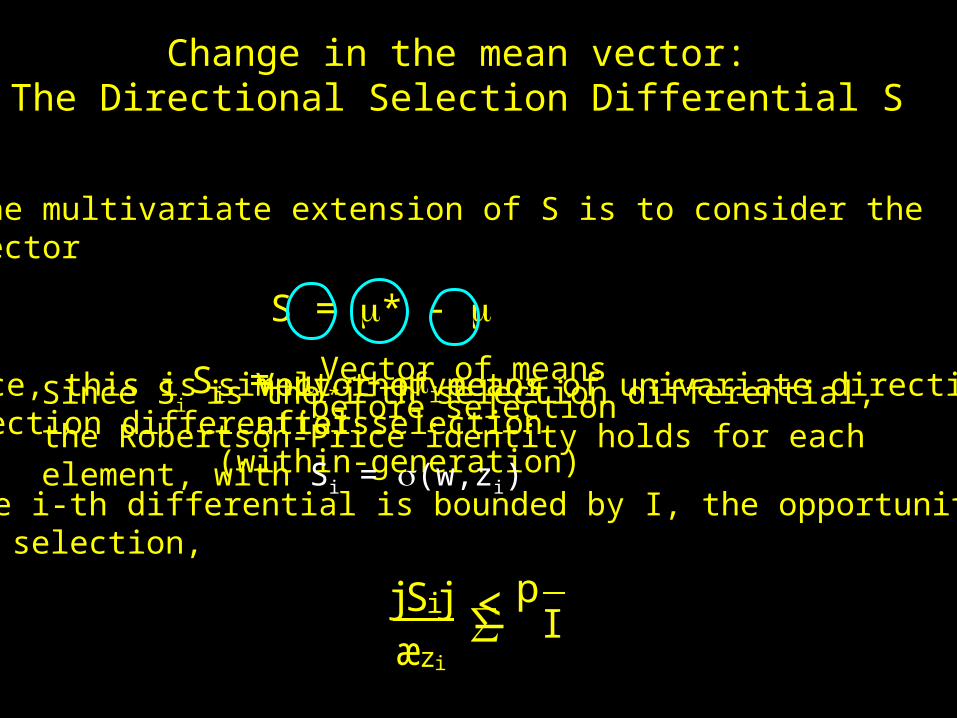
Change in the mean vector:The Directional Selection Differential S

The multivariate extension of S is to consider thevector

S = * -

Vector of meansbefore selection

Vector of meansafter selection

(within-generation)

Si = i* - iHence, this is simply the vector of univariate directionalSelection differentials

The i-th differential is bounded by I, the opportunityof selection,

jSi jæz i

∑p

I<

Since Si is the i-th selection differential, the Robertson-Price identity holds for each element, with Si = (w,zi)

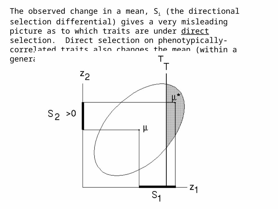
The observed change in a mean, Si (the directional selection differential) gives a very misleading picture as to which traits are under direct selection. Direct selection on phenotypically-correlated traits also changes the mean (within a generation).

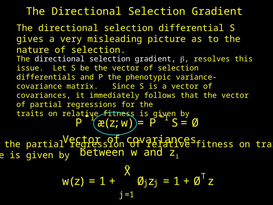
The Directional Selection Gradient

The directional selection differential S gives a very misleading picture as to the nature of selection.

The directional selection gradient, , resolves this issue. Let S be the vector of selection differentials and P the phenotypic variance-covariance matrix. Since S is a vector of covariances, it immediately follows that the vector of partial regressions for thetraits on relative fitness is given by

P °1æ(z;w) = P ° 1 S= Ø- -

Vector of covariancesbetween w and zi

Thus the partial regression of relative fitness on traitvalue is given by

w(z) = 1+nX

j=1

Øjzj = 1+ØT z

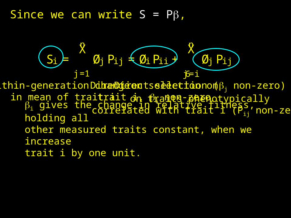
Since we can write S = P,

Si =nX

j=1

Øj P ij =Øi P ii +nX

j6=i

Øj P ij

Within-generation change in mean of trait i

Direction selection ontrait i, i non-zero

Direct selection (j non-zero)on traits phenotypically

correlated with trait i (Pij non-zero)i gives the change in relative fitness, holding allother measured traits constant, when we increasetrait i by one unit.

is a gradient vector on the meanfitness surface

Recall from vector calculus that the gradient operatoris given by

r xf (x) =

0

BB@

@f=@x1

@f=@x2...

@f=@xn

1

CCA

Ø = r π[lnW(π)] = W° 1

¢r π[W(π)]-

is the gradient (wrt the population mean) of themean fitness surface,

Hence, gives the direction the current mean shouldchange in to maximize the local change in mean fitness

is also the average gradient of the individual fitnesssurface over the phenotypic distribution,

Ø =Z

r z[w(z)] ¡(z)dz

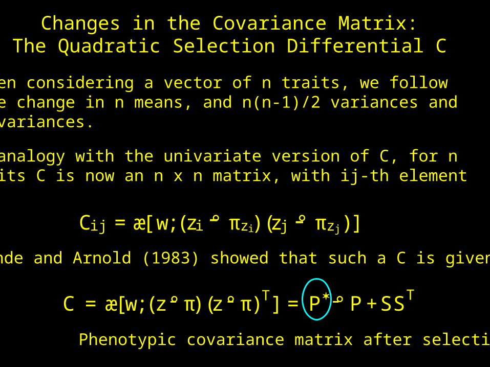
Changes in the Covariance Matrix:The Quadratic Selection Differential C

When considering a vector of n traits, we followthe change in n means, and n(n-1)/2 variances andcovariances.

By analogy with the univariate version of C, for ntraits C is now an n x n matrix, with ij-th element

C ij =æ[w;(zi ° πz i )(zj ° πz j )]- -Lande and Arnold (1983) showed that such a C is given by

C =æ[w;(z° π)(z° π)T ] = P ° P+SST-- -

Phenotypic covariance matrix after selection

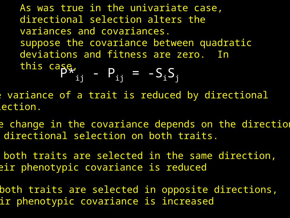
As was true in the univariate case, directional selection alters the variances and covariances.suppose the covariance between quadratic deviations and fitness are zero. In this case,

P*ij - Pij = -SiSj

The variance of a trait is reduced by directionalselection.

The change in the covariance depends on the directionof directional selection on both traits.

If both traits are selected in the same direction,their phenotypic covariance is reduced

If both traits are selected in opposite directions,their phenotypic covariance is increased

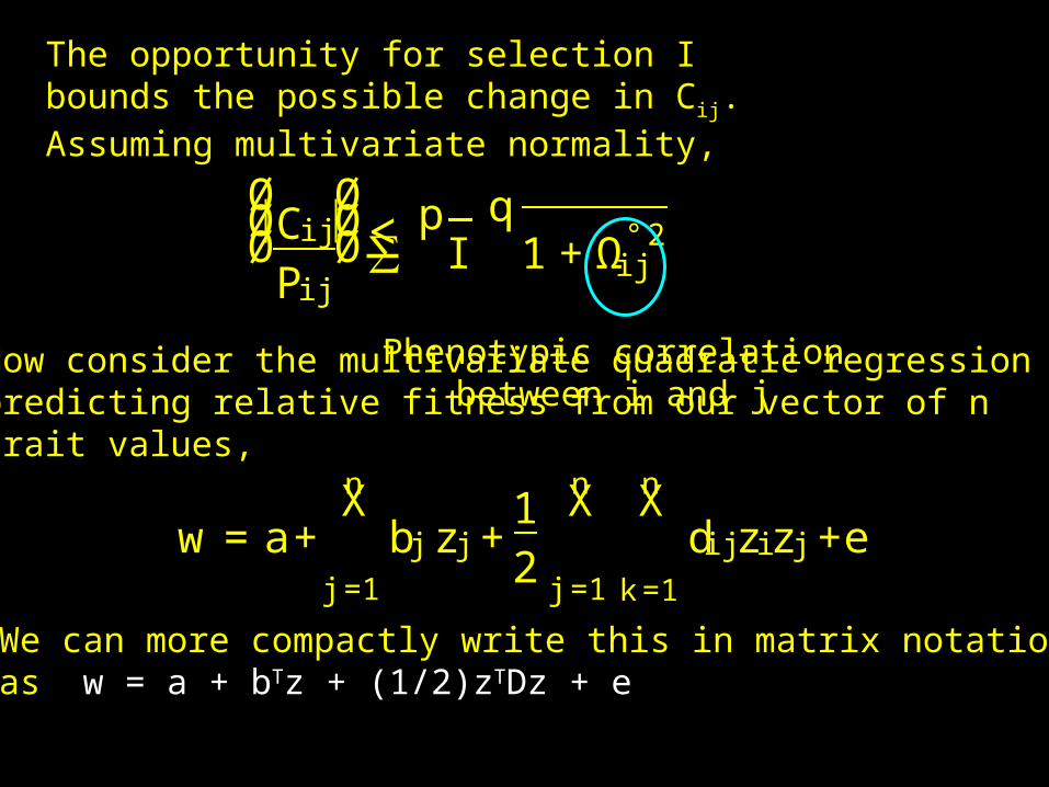
The opportunity for selection I bounds the possible change in Cij. Assuming multivariate normality,

ØØØC ij

P ij

ØØØ∑

pI

q1+Ω° 2

ij<

Phenotypic correlationbetween i and j

Now consider the multivariate quadratic regressionpredicting relative fitness from our vector of ntrait values,

w = a+nX

j=1

bj zj+12

nX

j=1

nX

k=1

dij zizj+e

We can more compactly write this in matrix notationas w = a + bTz + (1/2)zTDz + e

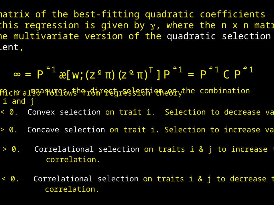
The matrix of the best-fitting quadratic coefficients in this regression is given by , where the n x n matrix is the multivariate version of the quadratic selectiongradient,

∞= P °1æ[w;(z° π)(z° π)T ] P ° 1 = P ° 1 C P ° 1-- - - - -

Which also follows from regression theory Here, ij measures the direct selection on the combinationof i and j• ii < 0. Convex selection on trait i. Selection to decrease variance

• ii > 0. Concave selection on trait i. Selection to increase variance

• ij > 0. Correlational selection on traits i & j to increase their correlation.

• ij < 0. Correlational selection on traits i & j to decrease their correlation.

While it has been very popular to infer the natureof quadratic selection directly from the individualij values, as we will shortly see, this can be verymisleading!

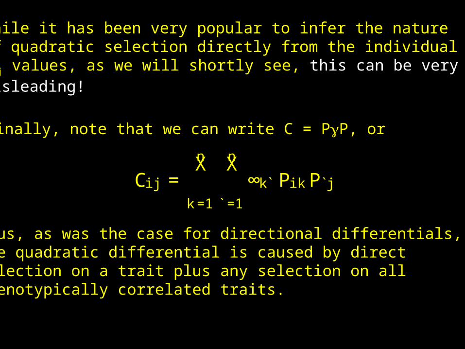
Finally, note that we can write C = PP, or

Thus, as was the case for directional differentials,the quadratic differential is caused by directselection on a trait plus any selection on all phenotypically correlated traits.

C ij =nX

k=1

nX

`=1

∞k` P ik P`j

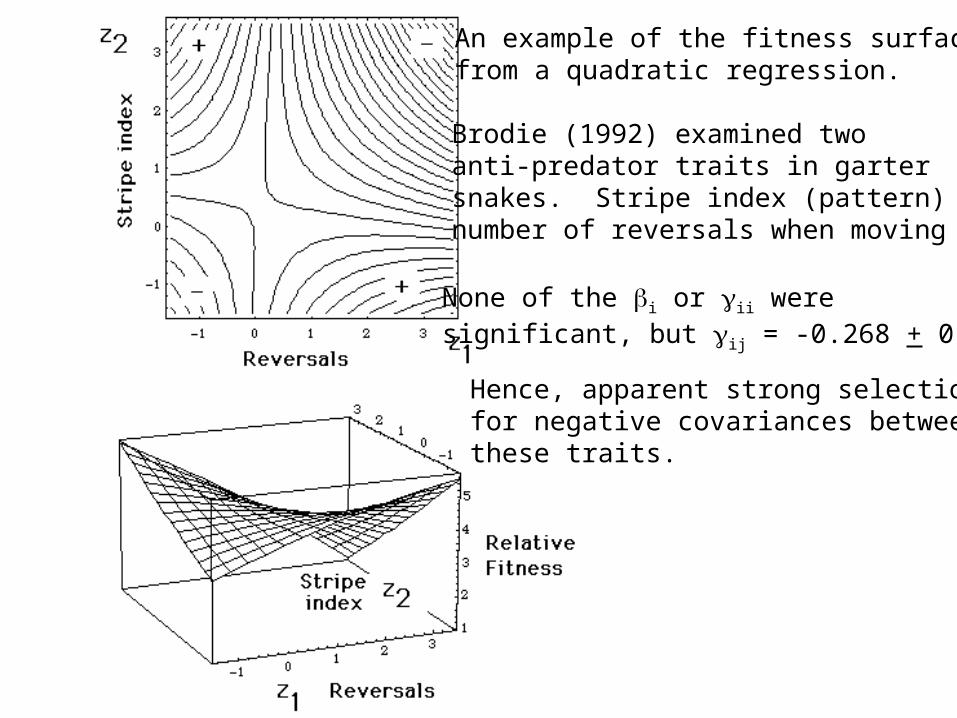
An example of the fitness surfacefrom a quadratic regression.

Brodie (1992) examined twoanti-predator traits in gartersnakes. Stripe index (pattern) andnumber of reversals when moving

Hence, apparent strong selection for negative covariances between these traits.

None of the i or ii weresignificant, but ij = -0.268 + 0.097

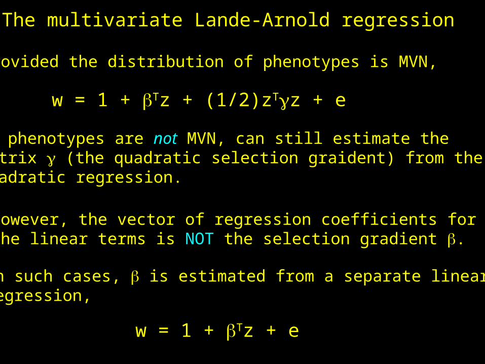
The multivariate Lande-Arnold regression

Provided the distribution of phenotypes is MVN,

w = 1 + Tz + (1/2)zTz + e

If phenotypes are not MVN, can still estimate thematrix (the quadratic selection graident) from the quadratic regression.

However, the vector of regression coefficients forthe linear terms is NOT the selection gradient .

In such cases, is estimated from a separate linearregression,

w = 1 + Tz + e

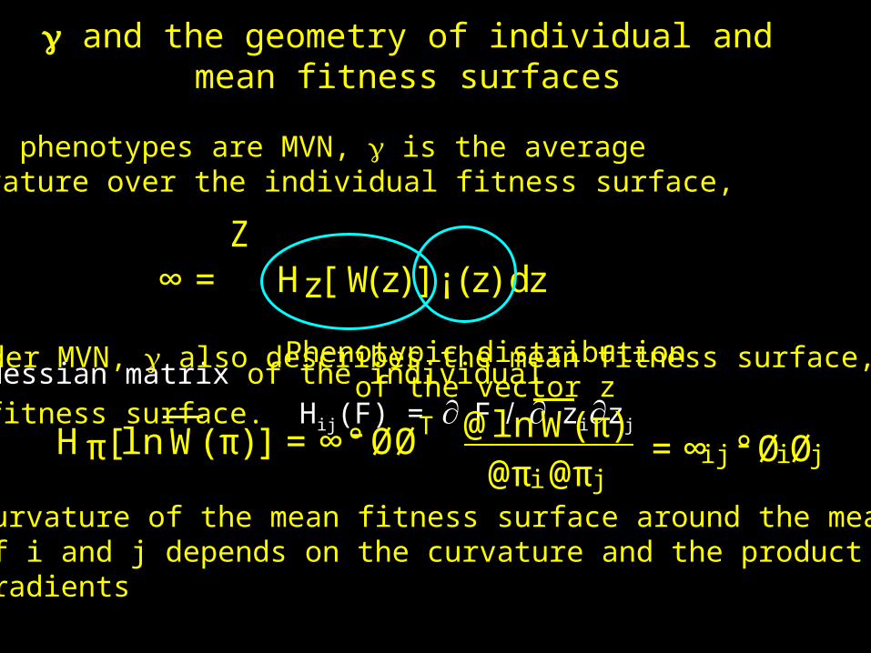
and the geometry of individual and mean fitness surfaces

When phenotypes are MVN, is the averagecurvature over the individual fitness surface,

∞=Z

Hz[W(z)] ¡(z)dz

Phenotypic distributionof the vector zHessian matrix of the individual

fitness surface. Hij(F) = Fzizj

Under MVN, also describes the mean fitness surface,

@lnW(π)@πi@π j

=∞ij °ØiØj-Hπ[lnW(π)] =∞°ØØT-

Curvature of the mean fitness surface around the meansof i and j depends on the curvature and the product ofgradients

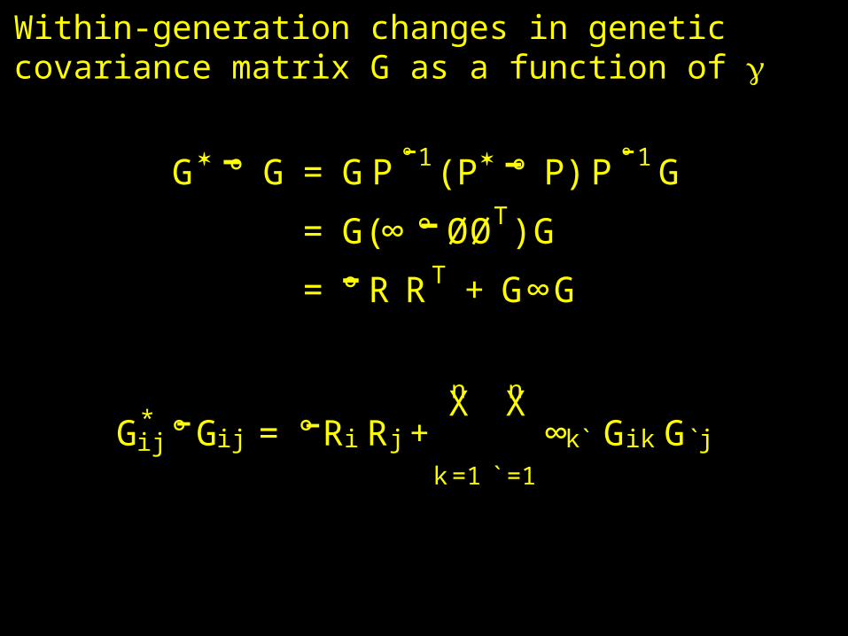
Within-generation changes in geneticcovariance matrix G as a function of

G ° G = GP ° 1 (P ° P) P ° 1G

= G(∞ ° ØØT )G

= ° R RT + G∞G

--

-

-

--

G*ij °G ij = ° R i R j+

nX

k=1

nX

`=1

∞k` Gik G`j- -

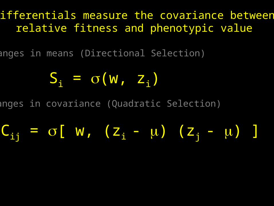
Changes in means (Directional Selection)

Changes in covariance (Quadratic Selection)

Differentials measure the covariance betweenrelative fitness and phenotypic value

Si = (w, zi)

Cij = [ w, (zi - ) (zj - ) ]

Changes in means (Directional Selection)

Changes in covariance (Quadratic Selection)

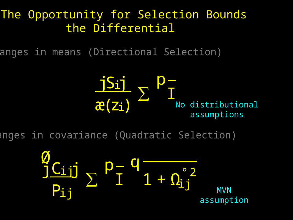
The Opportunity for Selection Boundsthe Differential

C ]qij =æ[w;(zi ° πi)(zj ° π j )ØC ij

P ij∑

pI 1+Ω° 2

ijj j

i =æ[w;zi ]jSi j

æ(zi)∑

pI

MVNassumption

No distributionalassumptions

Changes in means (Directional Selection)

Changes in covariance (Quadratic Selection)

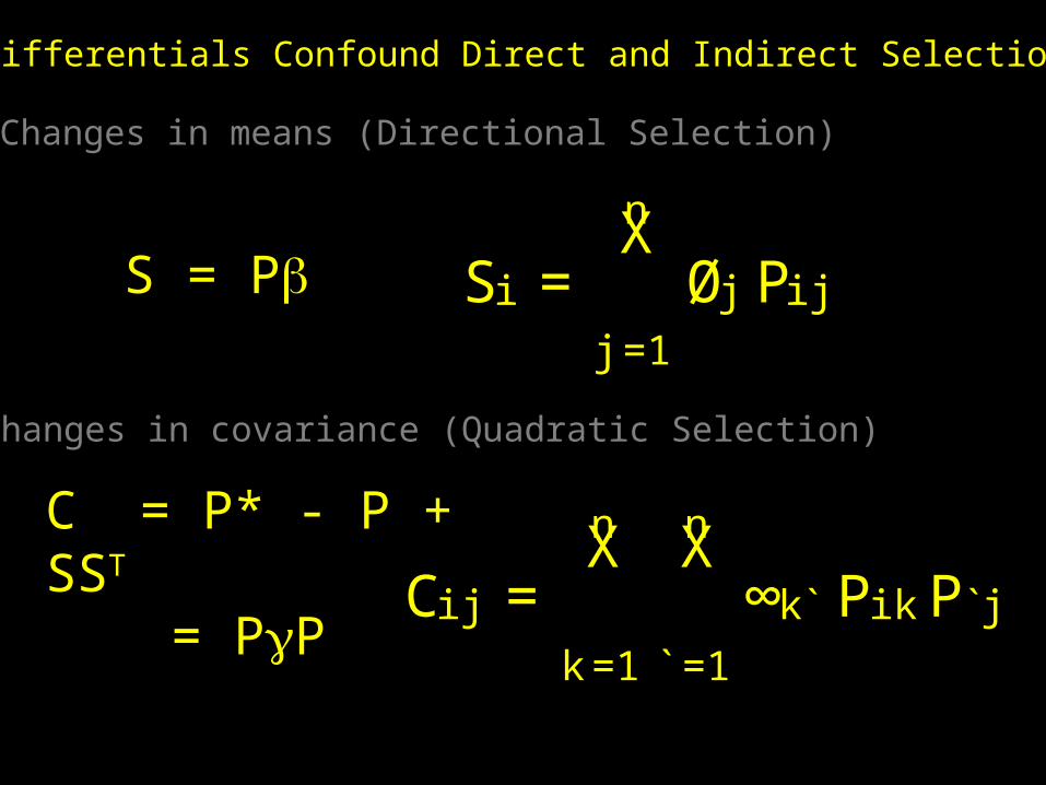
Differentials Confound Direct and Indirect Selection

C ij =nX

k=1

nX

`=1

∞k` P ik P`j

Si =nX

j=1

Øj P ijS = P

C = P* - P + SST

= PP

Changes in means (Directional Selection)

Changes in covariance (Quadratic Selection)

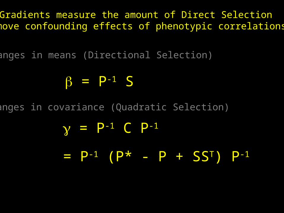
Gradients measure the amount of Direct Selection(remove confounding effects of phenotypic correlations)

= P-1 S

= P-1 C P-1

= P-1 (P* - P + SST) P-1

Changes in means (Directional Selection)

Changes in covariance (Quadratic Selection)

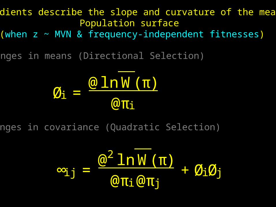
Gradients describe the slope and curvature of the meanPopulation surface

(when z ~ MVN & frequency-independent fitnesses)

Øi =@lnW(π)

@πi

∞ij =@2 lnW(π)

@πi@π j+ØiØj

Changes in means (Directional Selection)

Changes in covariance (Quadratic Selection)

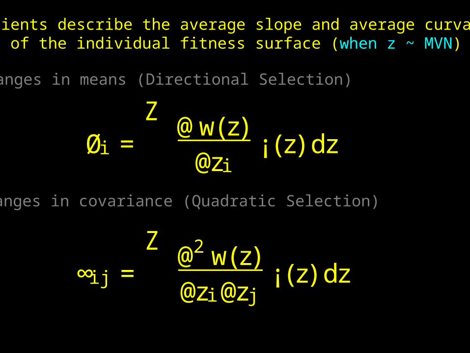
Gradients describe the average slope and average curvatureof the individual fitness surface (when z ~ MVN)

∞ij =Z

@2 w(z)@zi@zj

¡(z)dz

Øi =Z

@w(z)@zi

¡(z)dz

Changes in means (Directional Selection)

Changes in covariance (Quadratic Selection)

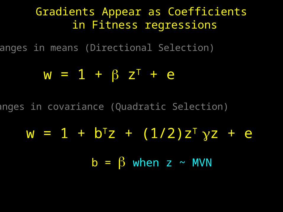
Gradients Appear as Coefficients in Fitness regressions

w = 1 + zT + e

w = 1 + bTz + (1/2)zT z + e

b = when z ~ MVN

Changes in means (Directional Selection)

Changes in covariance (Quadratic Selection)

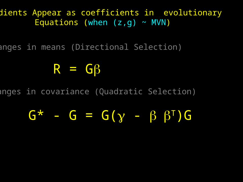
Gradients Appear as coefficients in evolutionaryEquations (when (z,g) ~ MVN)

R = G

G* - G = G( - T)G

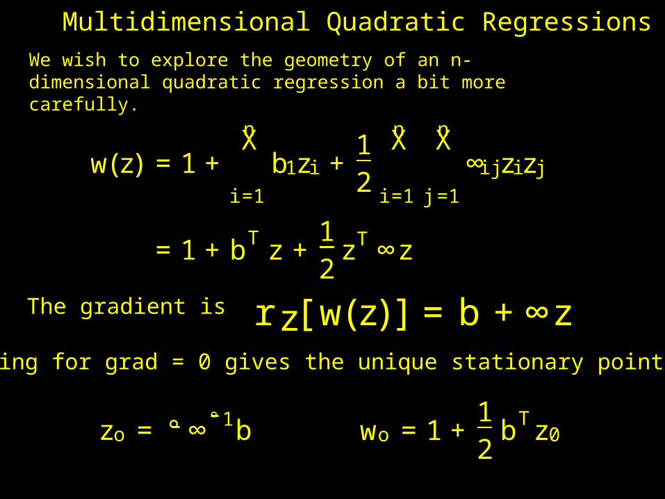
Multidimensional Quadratic RegressionsWe wish to explore the geometry of an n- dimensional quadratic regression a bit more carefully.

w(z) = 1+nX

i=1

b1zi +12

nX

i=1

nX

j=1

∞ij zizj

= 1+ bT z +12

zT ∞z

The gradient is r z[w(z)] = b +∞zSolving for grad = 0 gives the unique stationary point zo

wo = 1+12

bT z0zo = ° ∞° 1b- -

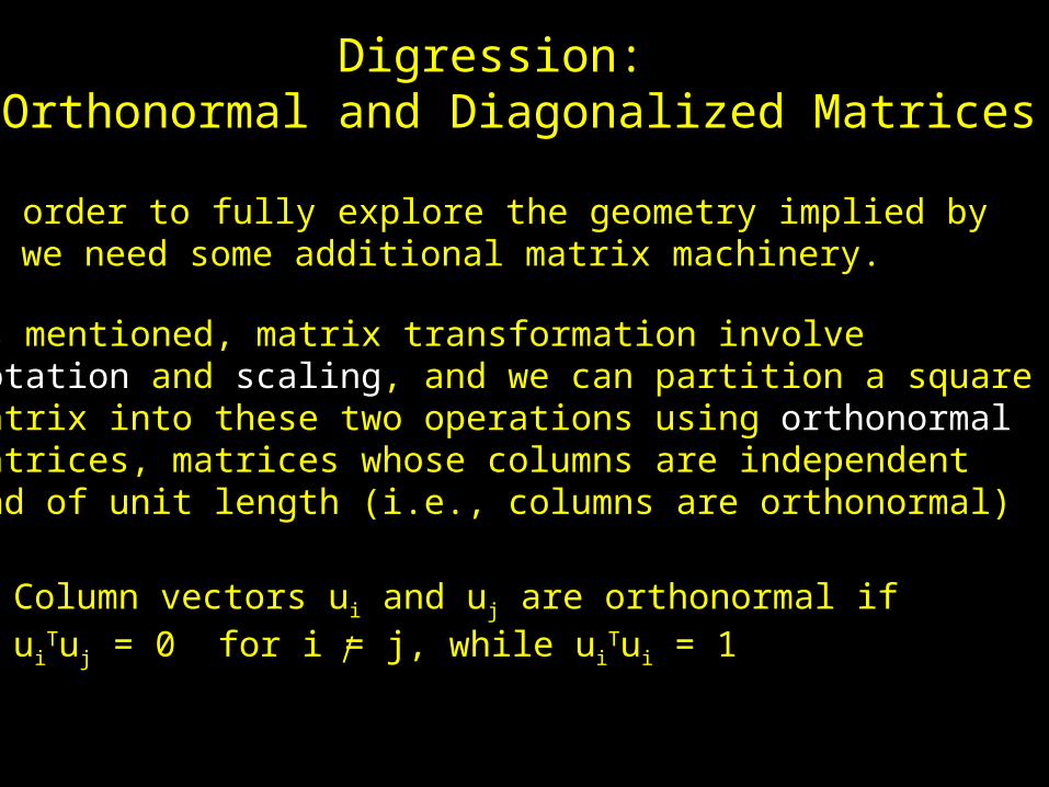
Digression: Orthonormal and Diagonalized Matrices

In order to fully explore the geometry implied by, we need some additional matrix machinery.

As mentioned, matrix transformation involverotation and scaling, and we can partition a squarematrix into these two operations using orthonormalmatrices, matrices whose columns are independentand of unit length (i.e., columns are orthonormal)

Column vectors ui and uj are orthonormal ifui

Tuj = 0 for i = j, while uiTui = 1

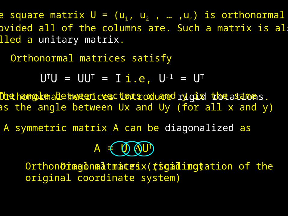
The square matrix U = (u1, u2 , … ,un) is orthonormalprovided all of the columns are. Such a matrix is alsocalled a unitary matrix.

Orthonormal matrices satisfy

UTU = UUT = I i.e, U-1 = UT

Orthonormal matrices introduce rigid rotations.The angle between vectors x and y is the sameas the angle between Ux and Uy (for all x and y)

A symmetric matrix A can be diagonalized as

A = U UT

Orthonormal matrices (rigid rotation of theoriginal coordinate system)

Diagonal matrix (scaling)

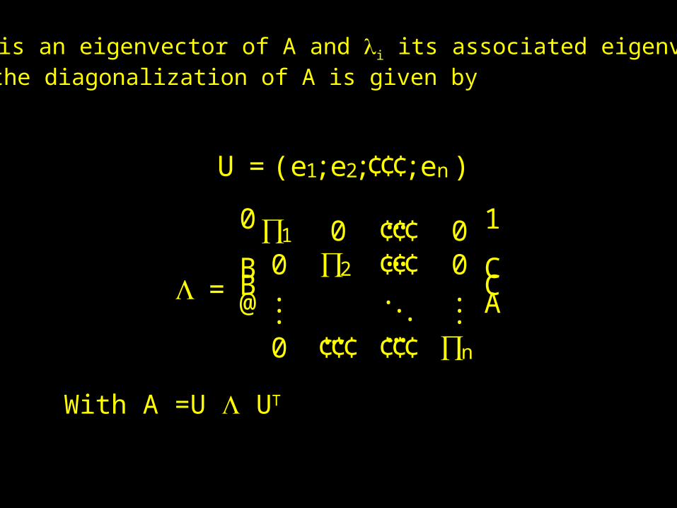
If ei is an eigenvector of A and i its associated eigenvalue,then the diagonalization of A is given by

U = (e1;e2;¢¢¢;en )

=

0

BB@

∏1 0 ¢¢¢ 00 ∏2 ¢¢¢ 0...

......

0 ¢¢¢ ¢¢¢ ∏n

1

CCA

… …

……

With A =U UT

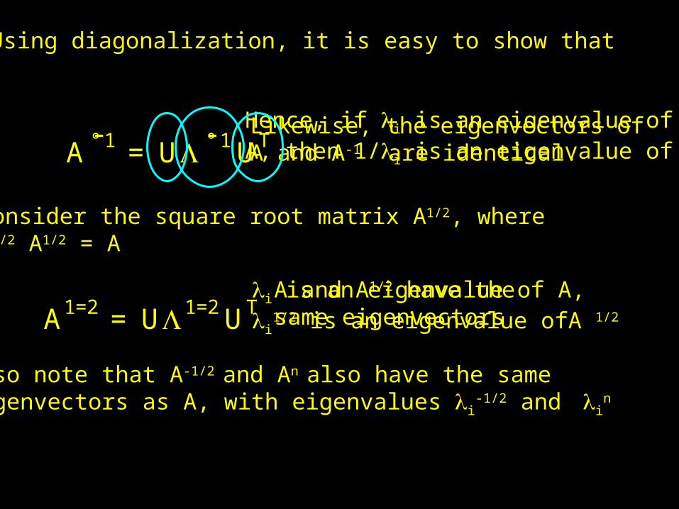
Using diagonalization, it is easy to show that

A1=2 = U1=2UT

A °1 = U ° 1UT- - Hence, if i is an eigenvalue ofA, then 1/i is an eigenvalue of A-1Likewise, the eigenvectors of A and A-1 are identical.

Consider the square root matrix A1/2, whereA1/2 A1/2 = A

i is an eigenvalue of A, i

1/2 is an eigenvalue ofA 1/2 A and A1/2 have the same eigenvectors

Also note that A-1/2 and An also have the same eigenvectors as A, with eigenvalues i

-1/2 and in

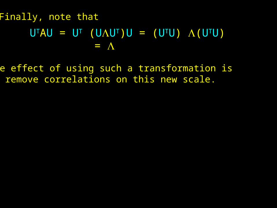
Finally, note that

UTAU = UT (UUT)U = (UTU) (UTU) =

The effect of using such a transformation isto remove correlations on this new scale.

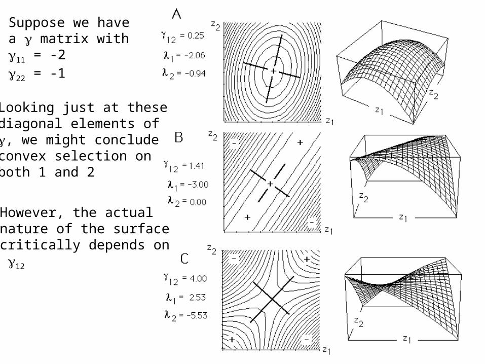
Suppose we havea matrix with 11 = -222 = -1

Looking just at thesediagonal elements of, we might concludeconvex selection onboth 1 and 2

However, the actualnature of the surfacecritically depends on 12

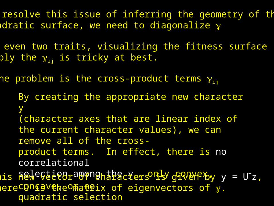
To resolve this issue of inferring the geometry of thequadratic surface, we need to diagonalize

For even two traits, visualizing the fitness surfacesimply the ij is tricky at best.

The problem is the cross-product terms ij

By creating the appropriate new character y(character axes that are linear index of the current character values), we can remove all of the cross-product terms. In effect, there is no correlationalselection among the yi, only convex, concave, or noquadratic selectionThis new vector of characters is given by y = UTz,

where U is the matrix of eigenvectors of .

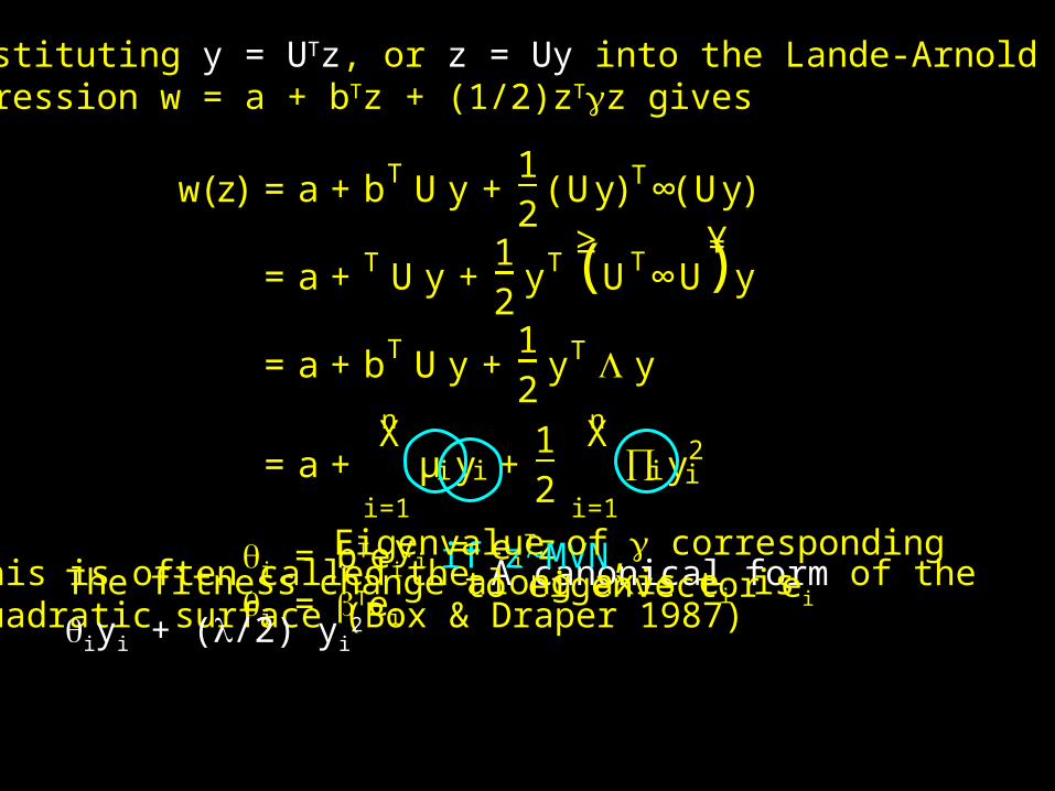
w(z) = a+ bT U y +12

(Uy)T∞(Uy)

= a+ T U y +12

yT≥

UT∞U¥

y

= a+ bT U y +12

yT y

= a+nX

i=1

µi yi +12

nX

i=1

∏i y2i

( )

Substituting y = UTz, or z = Uy into the Lande-Arnoldregression w = a + bTz + (1/2)zTz gives

This is often called the A canonical form of thequadratic surface (Box & Draper 1987)

yi = eiTzi = bTei

. if z~MVN, i = Tei

Eigenvalue of correspondingto eigenvector eiThe fitness change along axis ei is

iyi + (/2) yi2

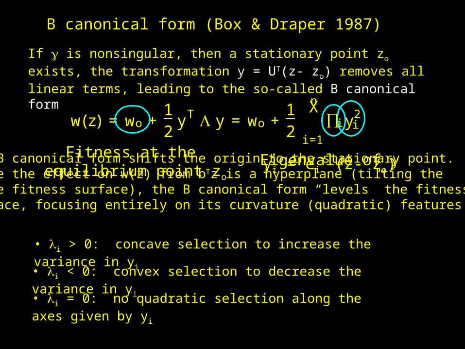
B canonical form (Box & Draper 1987)

If is nonsingular, then a stationary point zo exists, the transformation y = UT(z- zo) removes all linear terms, leading to the so-called B canonical form

w(z) = wo +12

yT y = wo +12

nX

i=1

∏i y2i

Fitness at the equilibrium point zo

yi = eiT (z- zo) Eigenvalue of The B canonical form shifts the origin to the stationary point.

Since the effect on w(z) from bTz is a hyperplane (tilting thewhole fitness surface), the B canonical form “levels” the fitnesssurface, focusing entirely on its curvature (quadratic) features.

• i > 0: concave selection to increase the variance in yi• i < 0: convex selection to decrease the variance in yi• i = 0: no quadratic selection along the axes given by yi

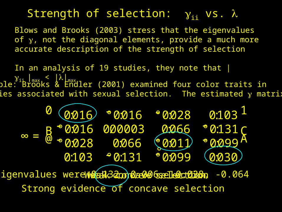
Strength of selection: ii vs. Blows and Brooks (2003) stress that the eigenvalues of , not the diagonal elements, provide a much more accurate description of the strength of selection

In an analysis of 19 studies, they note that | ii |max < ||max

Example: Brooks & Endler (2001) examined four color traits inguppies associated with sexual selection. The estimated matrix was

@

° °

A∞=

0

B0:016 °0:016 °0:028 0:103

°0:016 0:00003 0:066 °0:131°0:028 0:066 °0:011 °0:0990:103 0:131 0:099 0:030

1

C--

-

-

-

-°-

--

Weak concave selectionWeak convex selectionEigenvalues were 0.132, 0.006, -0.038, -0.064

Strong evidence of concave selection

Subspaces of

Blows & Brooks (2003) note that there are severaladvantages to focusing on estimation of the i vs.the entire matrix of ij.

First, there are n eigenvalues vs. n(n-1) elements of .

Further, many of the eigenvalues are likely close to 0,so that a subspace of (much like a subspace of G)describes most of the variation.

Blow & Brooks suggest obtaining the eigenvalues of ,and using these to generate transformed variablesy = UTz for those eigenvalues accounting for mostof the variation.

Note that the quadratic terms in the transformedregression on the y correspond to the eigenvalues,and hence GLM machinery can estimate theirstandard errors and confidence intervals.

Finally, Blows et al. (2004) suggest that one shouldconsider the projection of into G, just like weexamined the projection of into subspaces of G.

Here we are projecting a matrix instead of a vector,but the basic ideal holds.

First, construct a matrix B formed by a subset of ,namely the eigenvectors corresponding to k (< n/2)leading eigenvalues, B =(e1, …, ek)

Form a similar matrix with k eigenvectors of G

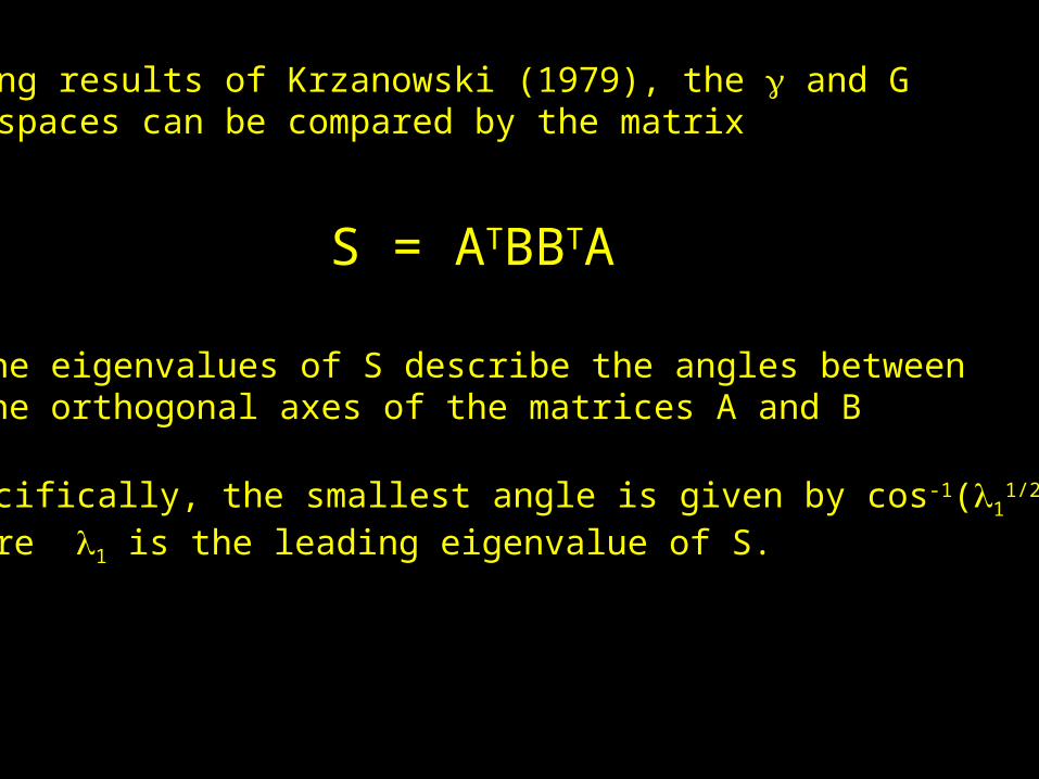
S = ATBBTA

Using results of Krzanowski (1979), the and G subspaces can be compared by the matrix

The eigenvalues of S describe the angles betweenthe orthogonal axes of the matrices A and B

Specifically, the smallest angle is given by cos-1(11/2 ),

where 1 is the leading eigenvalue of S.