measuring & modeling musical expressionpift6080/h08/documents/papers/eck... · 2008-12-04 ·...

1a

1b

International Laboratory forBrain, Music and Sound Research

International Laboratory forBrain, Music and Sound Research

PMS 7536 U

Measuring & Modeling Musical Expression

Douglas EckUniversity of Montreal

Department of Computer ScienceBRAMS Brain Music and Sound

Douglas Eck [email protected] / NIPS 2007 MBC Workshop

Overview

• Why care about timing and dynamics in music?

• Previous approaches to measuring timing and dynamics

• Models which predict something about expression

• Working without musical scores

• A correlation-based approach for constructing metrical trees

2

mailto:[email protected]



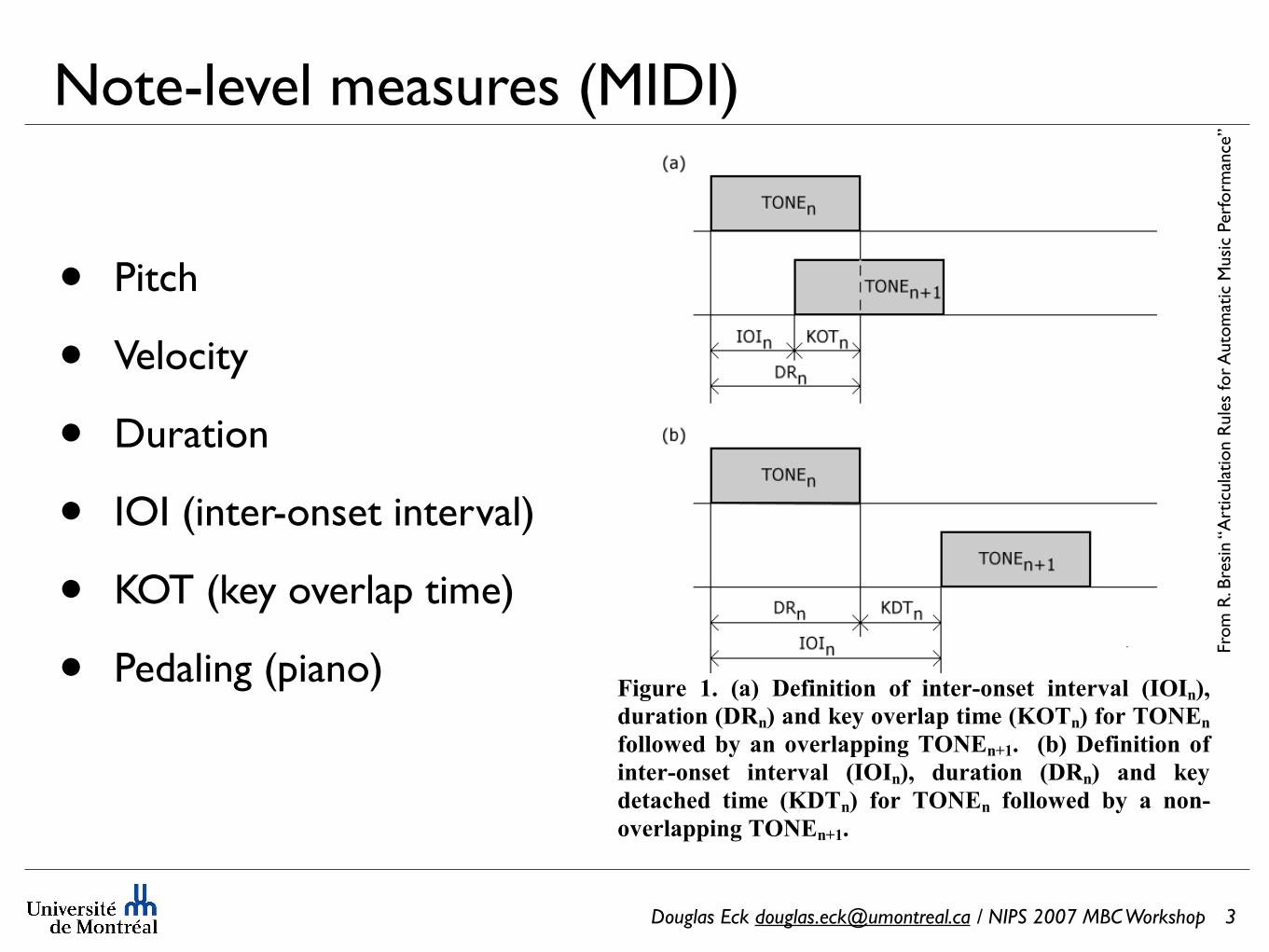
Note-level measures (MIDI)

• Pitch

• Velocity

• Duration

• IOI (inter-onset interval)

• KOT (key overlap time)

• Pedaling (piano)

3

!

!

!!"#$%&' ()' *+,' -&."/"0"1/' 1.' "/0&%21/3&0' "/0&%4+5' *676/,8'

9$%+0"1/'*-:/,'+/9';&<'14&%5+='0">&'*?7@/,'.1%'@7AB/'

.1551C&9'D<'+/'14&%5+=="/#'@7AB/E()' ' *D,'-&."/"0"1/'1.'

"/0&%21/3&0' "/0&%4+5' *676/,8' 9$%+0"1/' *-:/,' +/9' ;&<'

9&0+FG&9' 0">&' *?-@/,' .1%' @7AB/' .1551C&9' D<' +' /1/2

14&%5+=="/#'@7AB/E()'

H' I%0"F$5+0"1/':$5&3'"#! $%&'()*+! %&+&,%-.! /0! 1%&+(#! ,#2! 1,33&4! 567778! ,#2!

1%&+(#! ,#2! 9(2:&%! 567778;! :&,+*%&:&#3+! )<! 3.&!

$&%<)%:,#-&+!+3)%&2!(#!3.&!,/)'&=:&#3()#&2!2,3,/,+&+!>&%&!

+3,3(+3(-,440! ,#,40?&2@! A%):! 3.&+&! ,#,40+&+! 3.&! <)44)>(#B!

:,(#!%&+*43+!&:&%B&2C!5D8!EFG!(#!!"#$%&!#)3&+!(+!2&$&#2&#3!

<%):!"F"!)<! 3.&! <(%+3!)<! 3>)!)'&%4,$$(#B!#)3&+;! 568!EHG!(#!

'%$(($%&) #)3&+! (+! (#2&$&#2&#3! <%):! "F";! ,#2! 5I8! EHG! (#!

%&$&,3&2! #)3&+! (+! B&#&%,440! 2&$&#2&#3! <%):! "F"@! G.&+&!

%&+*43+! 4&2! 3)! 3.&! 2&<(#(3()#! )<! ,! #&>! +&3! )<! %*4&+! <)%!

,*3):,3(-! ,%3(-*4,3()#! (#! &J$%&++('&! $(,#)!:*+(-@! G.&! #&>!

%*4&+!,%&!<)*%@!G.&0!,%&!(#-4*2&2!(#!H(%&-3)%!K*+(-&+!5HK8;!

,! %*4&! +0+3&:! <)%! :*+(-! $&%<)%:,#-&! >%(33&#! (#! L)::)#!

M(+$! 4,#B*,B&! 5A%(/&%B;) "%) $!*! 67778@! N44! 3.&! ,%3(-*4,3()#!

%*4&+! -)#3%(/*3&! >(3.! 2(<<&%&#3! &<<&-3+! ,--)%2(#B! 3)!

&J$%&++('&! (#2(-,3()#+! 5<(%+3! 2,3,/,+&8;! 3&:$)! (#2(-,3()#+!

5+&-)#2! 2,3,/,+&C! $+$#,&;! $-+$-%";! $!!"#.&;! /."'%&0) ,#2!

1"-2"%%&8;! ,#2!,%3(-*4,3()#!:,%O+!>%(33&#! (#! 3.&! +-)%&@!G.&!

P3(&.")!"#$%&)$.%,(2!$%,&-4)%*4&!(+!,$$4(&2!3)!#)3&+!:,%O&2!

!"#$%&@!G.&!P3(&.")'%$(($%&)$.%,(2!$%,&-Q!%*4&!(+!,$$4(&2!3)!

#)3&+!:,%O&2!'%$(($%&@!G.&!P5.%,(2!$%,&-)&6)."/"%,%,&-Q!%*4&!

(#+&%3+! ,! :(-%)$,*+&! /&3>&&#! 3>)! -)#+&-*3('&! 3)#&+! >(3.!

3.&! +,:&! $(3-.@! G.&! P72.$%,&-) (&-%.$'%) $.%,(2!$%,&-4! %*4&!

-,#!/&!*+&2!3)!-)#3%)4!3.&!30$&!)<!,%3(-*4,3()#;!%,#B(#B!<%):!

'%$(($%&) 3)! !"#$%&0! )<! #)3&+! 3.,3! ,%&!:,%O&2! #&(3.&%! !"#$%&!

#)%! '%$(($%&@! "#! 3.&! #&J3! $,%,B%,$.+! ,! 2&+-%($3()#! )<! 3.&+&!

%*4&+! (+! $%)'(2&2@! "3! <)44)>+! 3.&! <)%:,3! *+&2! (#! 3.&! HK!

2)-*:&#3,3()#!5<)%!:)%&!(#<)%:,3()#!+&&!3.&!4(+3!)<!4(#O+!,3!

$,%,B%,$.!R8@!

H)(' JF1%&'5&#+01'+%0"F$5+0"1/'%$5&'

78)9,'/)62-(%,&-)-$1"S!T-)%&=4&B,3)=,%3@!

7"'(.,/%,&-S! 3.(+! %*4&! $%)2*-&+! ,#! )'&%4,$! )<! 3)#&+;! )%!

!"#$%&@!G.&!$+&*2)-)2&!)<!3.&!%*4&!(+!$%&+&#3&2!/&4)>@!

566"(%"+)'&2-+)/$.$1"%".S!O&0!)'&%4,$!3(:&;!EFG)U:+V@!

:'$#") $-+) !,1,%$%,&-';! 3.&! %*4&! -,#! /&! *+&2! 3)! -)#3%)4! 3.&!

W*,#3(30!)<! !"#$%&),%3(-*4,3()#@! "3! (+! ,$$4(&2! 3)!#)3&+! 3.,3!

,%&!:,%O&2!!"#$%&)(#!3.&!+-)%&;!,+!+*BB&+3&2!/0!3.&!#,:&!

)<!3.&!%*4&@!X%)*$+!)<!!"#$%&)#)3&+!,%&!:,%O&2!(#!3.&!+-)%&!

<(4&!>(3.!3.&!M(+$!-)::,#2+!(LEGATO-START T)!,#2!(LEGATO-END T)@! 5T&&! 3.&! HK! 2)-*:&#3,3()#! <)%!(#<)%:,3()#! ,/)*3! 3.&! +-)%&! <)%:,3! ,#2! 3.&! M(+$!

-)::,#2+!,',(4,/4&8@!

Y+&*2)-)2&!<)%!3.&!3(&.")9"#$%&)5.%,(2!$%,&-)%*4&S!

".''D!P!<!PZ!R!

0G&/''<=>)!!557@R[D7=\[<)=!7@DDD7

=I8[?=?]!7@7DD7R[<)]!

]!7@D\7\I8[?=?!

&53&''".''7!P!<!PZ!D!

0G&/''<=>)!!55=^@I[D7=\[<)=!\@\[D7

=\8[?=?)@)

]!R_@RII[D7=I[<)]!DDI@DR[D7

=I8[?=?!

>.&%&! E! (+! ,! >&(B.3(#B! $,%,:&3&%! 2&3&%:(#(#B! 3.&!

:,B#(3*2&!)<!EFG@!!

G.&! E! ',4*&+! -,#! /&! ,++)-(,3&2! >(3.! 3.&! 2(<<&%&#3!

$4,0(#B! +304&+! -)%%&+$)#2(#B! 3)! 3.&! ,2`&-3('&+! *+&2! <)%! 3.&!

&J$&%(:&#3!2&+-%(/&2!(#!,!%&-&#3!>)%O!/0!1%&+(#!,#2!1,33&4!

567778S!

<!Z!R! ZZQ! $,++()#,3&!!"#$%&!!

<!Z!D! ZZQ! #,3*%,4!!"#$%&)!

<!Z!7@D! ZZQ! <4,3!!"#$%&))

"3!:&,#+!3.,3!/0!',%0(#B!3.&!&:$.,+(+!$,%,:&3&%!E!<%):!

7@D! 3)! R! (3! >(44! /&! $)++(/4&! 3)! +>&&$! 3.%)*B.! ,! ',%(&30! )<!

!"#$%&)+304&+@!

H)K' JF1%&'30+FF+01'+%0"F$5+0"1/'%$5&'

78)9,'/)62-(%,&-)-$1"S!T-)%&=+3,--,3)=,%3@!

7"'(.,/%,&-S! 3.(+! %*4&! (#3%)2*-&+! ,! :(-%)$,*+&! ,<3&%! ,!

'%$(($%&) 3)#&@! G.&! $+&*2)-)2&! )<! 3.&! %*4&! (+! $%&+&#3&2!

/&4)>@!

566"(%"+)'&2-+)/$.$1"%".S!O&0!2&3,-.&2!3(:&;!EHG)U:+V@!

:'$#") $-+) !,1,%$%,&-';! 3.&! %*4&! -,#! /&! *+&2! 3)! -)#3%)4! 3.&!

W*,#3(30! )<! '%$(($%&) ,%3(-*4,3()#@! "3! (+! ,$$4(&2! 3)! #)3&+!

:,%O&2!'%$(($%&)(#!3.&!+-)%&;!,+!+*BB&+3&2!/0!3.&!#,:&!)<!

3.&! %*4&@! 3%$(($%&! (+! :,%O&2! (#! 3.&! +-)%&! >(3.! 3.&! M(+$!

-)::,#2!(STACCATO T)@!N#!&J3%,!$,%,:&3&%;!>"1/&A,-+,($%,&-;! -,#!/&!*+&2! 3)! ,-.(&'&!2(<<&%&#3! W*,#3(3(&+! )<!

'%$(($%&! <)%! 2(<<&%&#3! %"1/&) (#2(-,3()#+@! G.&! HK!

-)::,#2! 4(#&! <)%! 3.&!3(&.")3%$(($%&)5.%,(2!$%,&-)%*4&! (+!

3.&%&<)%&S!

T-)%&=+3,--,3)=,%3!P<Q!SG&:$)=(#2(-,3()#!B%"1/&4!

>.&%&! %"1/&) (+! 3.&! *+&%! (#$*3! ',4*&! <)%! 3.&! G&:$)=

(#2(-,3()#!',%(,/4&@!

From

R. B

resi

n “A

rtic

ulat

ion

Rul

es fo

r Aut

omat

ic M

usic

Per

form

ance

”



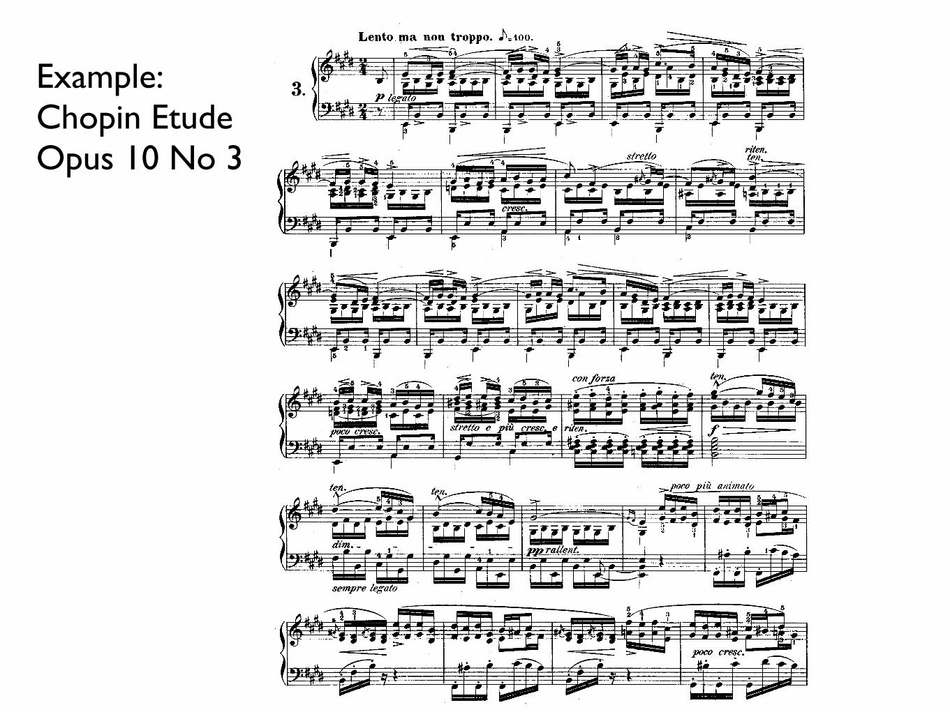
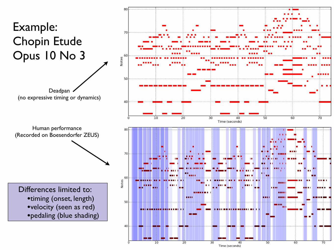
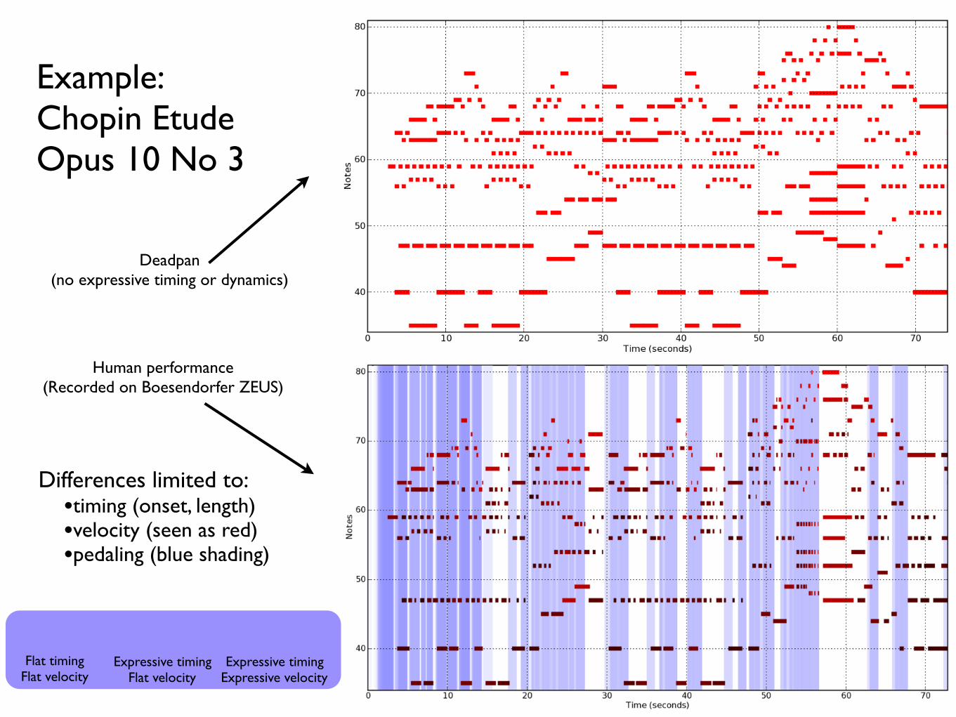
Example: Chopin Etude Opus 10 No 3


Deadpan (no expressive timing or dynamics)

Human performance (Recorded on Boesendorfer ZEUS)

Differences limited to:•timing (onset, length)•velocity (seen as red)•pedaling (blue shading)


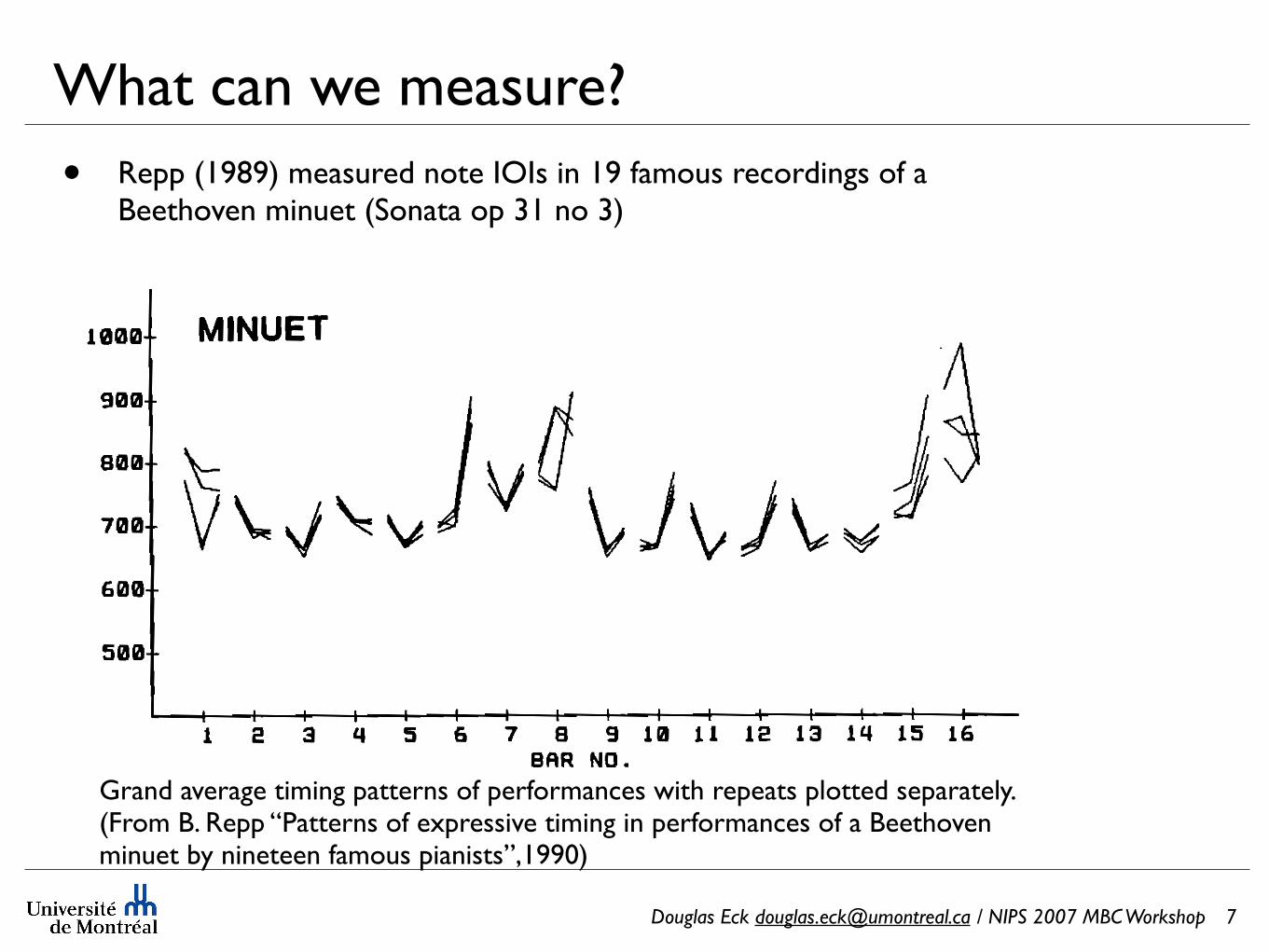
What can we measure?• Repp (1989) measured note IOIs in 19 famous recordings of a

Beethoven minuet (Sonata op 31 no 3)

7

o

u

R

T

!

0

N

!

N

1ooo

?00

600

500.

9cq•-

880-

70•-

600.

100•*

900.

800-

7•.

600.

MINUET

! I I I [ I I [ I I I I I • I I I E: 3 q 5 6 7 8 9 18 t! 1• 13 ,tq t5 16 BRR NO.

TRIO

I I I I I I I I I I I I I t7 18 19 aO Et EE E3 Eq •5 g6 •7 a8 •9 30 31 3E 33 3q 35 36 37 38

BRR NO.

CODA

I I I I I I I 39 qa qt qE q3 qq q5

BRR ND.

FIG. 3. Grandaveragetimingpatternof15human •fformances, withre•atsplott• separately. Thel•ton•t-on•tintervalintheCoda(arrow)is1538 ms.

I. Repeats

It is evident, first, that repeats of the same material had extremely similar timing patterns. This consistency of pro- fessional keyboard players with respect to detailed timing patterns has been noted many times in the literature, beginning with Seashore ( 1938, p. 244). The only systematic deviations occurred in bar 1 and at phrase endings (bars 8, 15- 16, and 23/37-24/38), where the music was, in fact, not identical across repeats (see Fig. 1): In bar 1, Beethoven added an ornament (a turn on E-flat) in the repeat (bar 1B), which was slightly drawn out by most pianists. In bar 8A,

which led back to the beginning of the Minuet, the upbeat was prolonged, but in bar 8B, which led into the second section of the Minuet, an additional ritard occurred on the phrase-final (second) beat. Similarly, a uniform ritard was produced in bar 16A, which led back to the beginning of the second Minuet section, and an even stronger ritard occurred on the phrase-final (first and second) notes of bar 16B, which constituted the end of the Minuet, whereas the third note constituted the upbeat to the Trio and was taken shorter. Bar 15 anticipated these changes, which were more pronounced in the second playing of the Minuet, following the Trio. Similarly, bar 37 anticipated the large ritard in bar

628 J. Acoust. Sec. Am., Vol. 88, No. 2, August 1990 Bruno H. Repp: Expressive timing in a Beethoven minuet 628

Grand average timing patterns of performances with repeats plotted separately. (From B. Repp “Patterns of expressive timing in performances of a Beethoven minuet by nineteen famous pianists”,1990)




What can we measure?

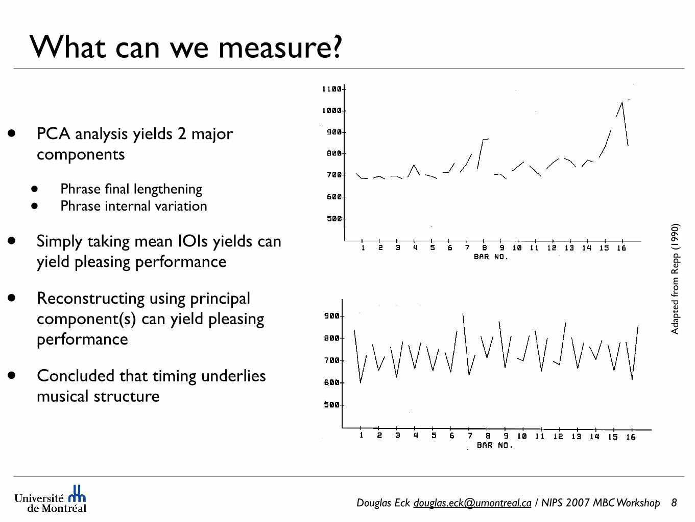
• PCA analysis yields 2 major components

• Phrase final lengthening• Phrase internal variation

• Simply taking mean IOIs yields can yield pleasing performance

• Reconstructing using principal component(s) can yield pleasing performance

• Concluded that timing underlies musical structure

8

Ada

pted

from

Rep

p (1

990)

•L00-

•000-

600-

B00-

700-

600-

500-

FACTOR I

I I I I I I I I

I E 3 q 5 6 7 8

BRR

I I I I I I I

9 10 11 1E 13 lq 15 16

NO.

D

U

R

T

I

O

N

I

N

800

788-

608-

580-

900-

088-

708-

608-

500-

FACTOR 2

./

I I I I I I I I I I I I I I I I

I E :3 q 5 6 7 8 El 18 11 1E 13 lq 15

BRR NO,

FACTOR 3

I [ I I I I I I I I I I I I I I I E 3 q 5 6 7 8 9 10 11 IE 13 tq 15 16

BRR NO,

were quite rare in the present composition. Eighth-notes were common but provided less information, since they re-

duced the four-beat pulse to a two-beat pulse. Some measurement problems were also encountered. Nevertheless,

some data were obtained about the temporal microstructure at this level.

A. Sixteenth-notes

1. Measurement procedures

Sequences of two sixteenth-notes occur in several places (bars 7, 20, and 34), but proved very difficult to measure; the

onset of the second note could usually not be found in the acoustic waveform. Therefore, the measurements were re-

stricted to single sixteenth-notes following a dotted eighth- note. Such notes occur in bars 0/8A, 1, 4, and 8B/16A of the

Minuet, in bar 23/37 of the Trio, and throughout the Coda. With four repeats of the Minuet and two of the Trio in most

performances, there were generally four independent measures available for each of the four sixteenth-note occur-

rences in the Minuet and for the single occurrence in the Trio

(the latter really being two similar occurrences, each repeated twice). For the Coda, of course, only a single set of measurements was available for each artist, but there were 11


•L00-

•000-

600-

B00-

700-

600-

500-

FACTOR I

I I I I I I I I

I E 3 q 5 6 7 8

BRR

I I I I I I I

9 10 11 1E 13 lq 15 16

NO.

D

U

R

T

I

O

N

I

N

800

788-

608-

580-

900-

088-

708-

608-

500-

FACTOR 2

./

I I I I I I I I I I I I I I I I

I E :3 q 5 6 7 8 El 18 11 1E 13 lq 15

BRR NO,

FACTOR 3

I [ I I I I I I I I I I I I I I I E 3 q 5 6 7 8 9 10 11 IE 13 tq 15 16

BRR NO,

were quite rare in the present composition. Eighth-notes were common but provided less information, since they re-

duced the four-beat pulse to a two-beat pulse. Some measurement problems were also encountered. Nevertheless,

some data were obtained about the temporal microstructure at this level.

A. Sixteenth-notes

1. Measurement procedures

Sequences of two sixteenth-notes occur in several places (bars 7, 20, and 34), but proved very difficult to measure; the

onset of the second note could usually not be found in the acoustic waveform. Therefore, the measurements were re-

stricted to single sixteenth-notes following a dotted eighth- note. Such notes occur in bars 0/8A, 1, 4, and 8B/16A of the

Minuet, in bar 23/37 of the Trio, and throughout the Coda. With four repeats of the Minuet and two of the Trio in most

performances, there were generally four independent measures available for each of the four sixteenth-note occur-

rences in the Minuet and for the single occurrence in the Trio

(the latter really being two similar occurrences, each repeated twice). For the Coda, of course, only a single set of measurements was available for each artist, but there were 11





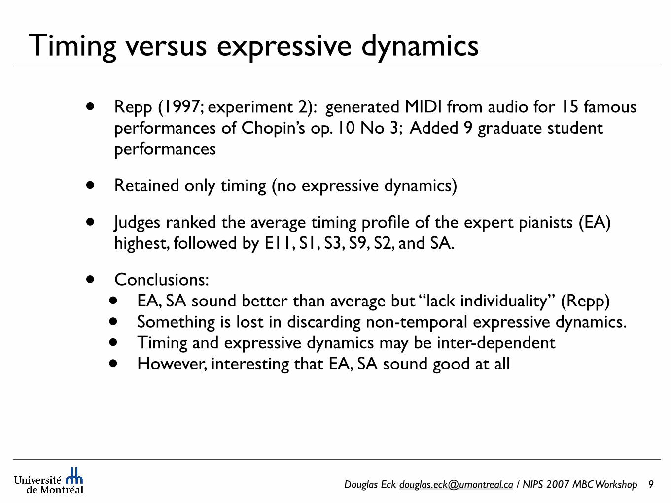
Timing versus expressive dynamics

• Repp (1997; experiment 2): generated MIDI from audio for 15 famous performances of Chopin’s op. 10 No 3; Added 9 graduate student performances

• Retained only timing (no expressive dynamics)

• Judges ranked the average timing profile of the expert pianists (EA) highest, followed by E11, S1, S3, S9, S2, and SA.

• Conclusions:• EA, SA sound better than average but “lack individuality” (Repp)• Something is lost in discarding non-temporal expressive dynamics. • Timing and expressive dynamics may be inter-dependent• However, interesting that EA, SA sound good at all

9




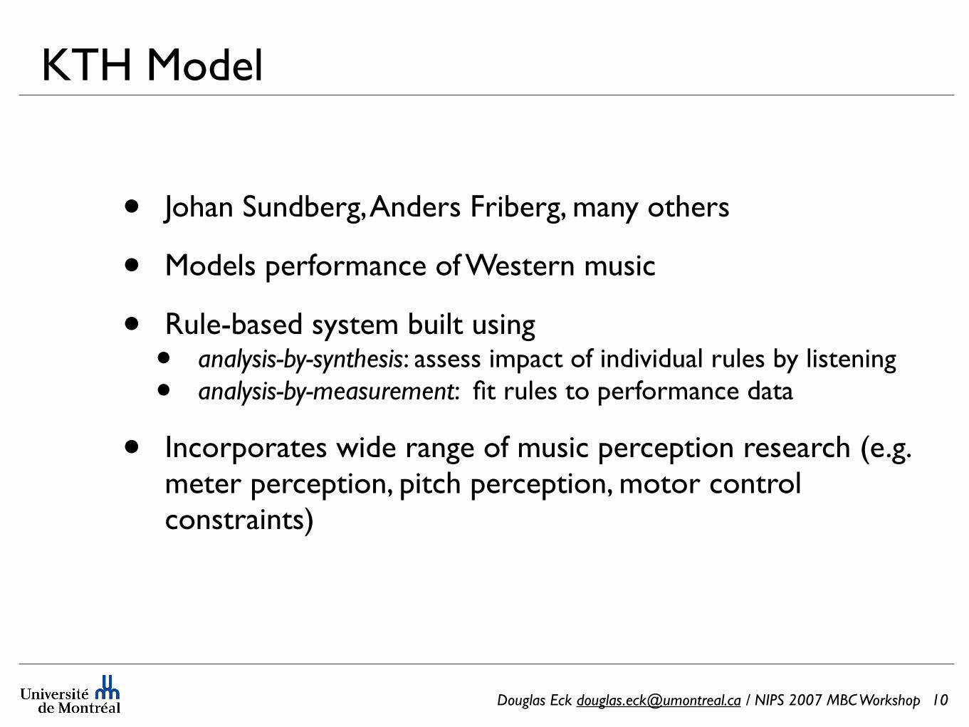
KTH Model

• Johan Sundberg, Anders Friberg, many others

• Models performance of Western music

• Rule-based system built using • analysis-by-synthesis: assess impact of individual rules by listening• analysis-by-measurement: fit rules to performance data

• Incorporates wide range of music perception research (e.g. meter perception, pitch perception, motor control constraints)

10



148

http://www.ac-psych.org

Anders Friberg, Roberto Bresin, and Johan Sundberg

1994; Desain & Honing, 1994; Honing, 2005a). For most

of the rules, our starting point has been to implement

expressive deviations relative to the tempo, i.e. analo-

gous to Weber’s law2. This approach works well within a

tempo range when note durations are not too short3. The

most notable exceptions are the rules Duration contrast

and Swing ensemble, described below.

The role of performance marks such as accents or

phrase marks in the score may also be considered.

These marks are often treated more as a guideline for

the performance than mandatory ways of performing

the piece. Furthermore, these marks are often inserted

by the editor rather than the composer. Therefore, we

have in general avoided incorporating such marks in

the score, thus, mainly trying to model the perform-

ance from the “raw” score. One exception is the set of

rules for notated staccato/legato.

Certain aspects of musical structure must be pro-

vided manually by the user because they are not

readily evident from surface properties. For example,

automatic extraction of phrase structure and harmonic

structure is a difficult process (Temperley, 2001;

Ahlbäck, 2004), but these analyses are essential for

the phrasing and tonal tension rules respectively. Thus,

these structural characteristics must be added to the

score manually by the user so that they can trigger the

phrasing and tonal tension rules. One exception is the

rule for musical punctuation, which automatically finds

the melodic grouping structure on a lower level.

Because the rules act upon a range of structural

characteristics of music, they provide an expressive

interpretation of musical structure. An analogous func-

tion is observed in speech prosody, which introduces

variation in a range of acoustic features (intensity,

Phrasing

Phrase arch Create arch-like tempo and sound level changes over phrases

Final ritardando Apply a ritardando in the end of the piece

High loud Increase sound level in proportion to pitch height

Micro-level timing

Duration contrast Shorten relatively short notes and lengthen relatively long notes

Faster uphill Increase tempo in rising pitch sequences

Metrical patterns and grooves

Double duration Decrease duration ratio for two notes with a nominal value of 2:1

Inégales Introduce long-short patterns for equal note values (swing)

Articulation

Punctuation Find short melodic fragments and mark them with a final micropause

Score legato/staccato Articulate legato/staccato when marked in the score

Repetition articulation Add articulation for repeated notes.

Overall articulation Add articulation for all notes except very short ones

Tonal tension

Melodic charge Emphasize the melodic tension of notes relatively the current chord

Harmonic charge Emphasize the harmonic tension of chords relatively the key

Chromatic charge Emphasize regions of small pitch changes

Intonation

High sharp Stretch all intervals in proportion to size

Melodic intonation Intonate according to melodic context

Harmonic intonation Intonate according to harmonic context

Mixed intonation Intonate using a combination of melodic and harmonic intonation

Ensemble timing

Melodic sync Synchronize using a new voice containing all relevant onsets

Ensemble swing Introduce metrical timing patterns for the instruments in a jazz ensemble

Performance noise

Noise control Simulate inaccuracies in motor

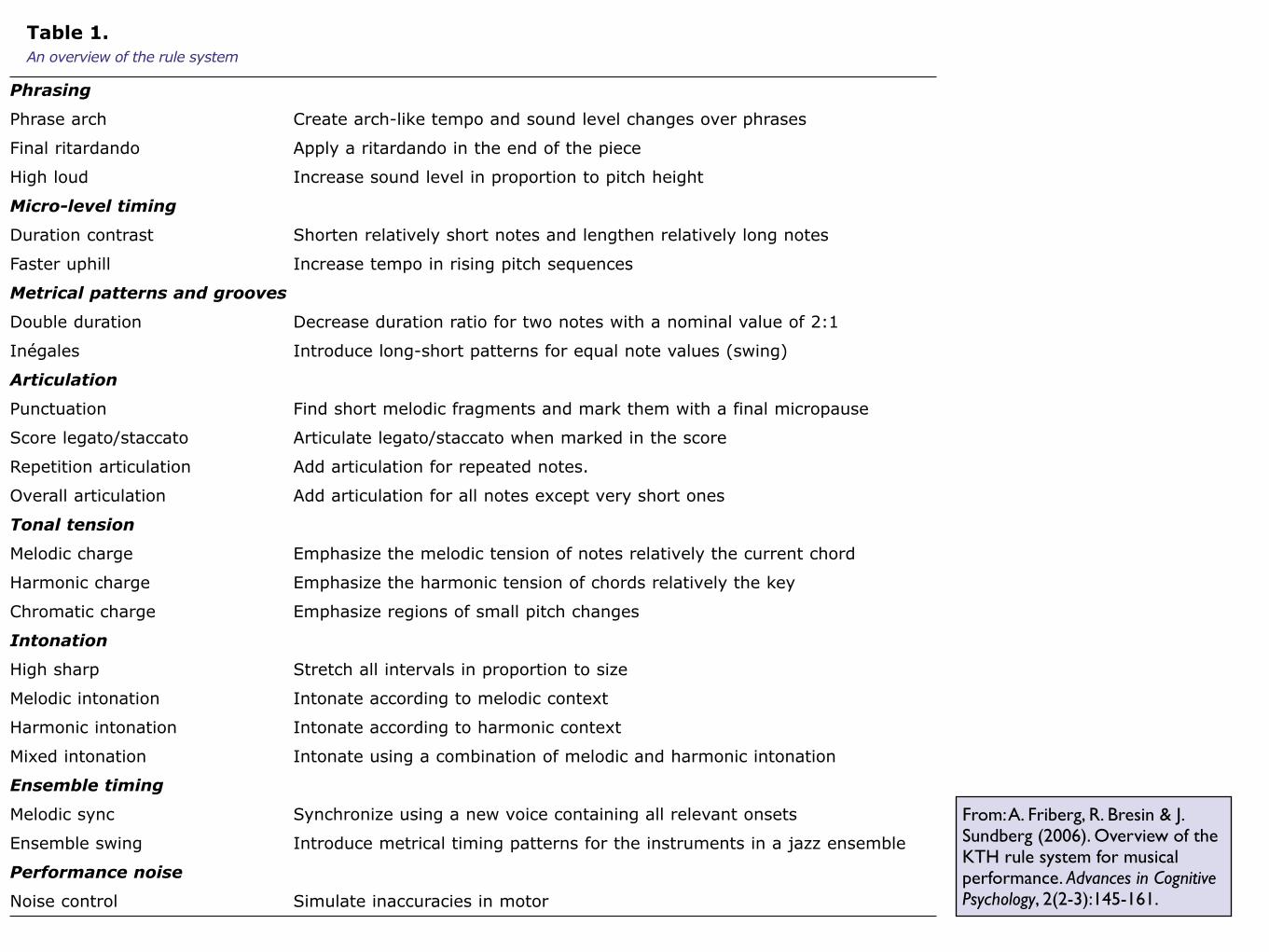
Table 1.

An overview of the rule system

From: A. Friberg, R. Bresin & J. Sundberg (2006). Overview of the KTH rule system for musical performance. Advances in Cognitive Psychology, 2(2-3):145-161.

From: A. Friberg, R. Bresin & J. Sundberg (2006). Overview of the KTH rule system for musical performance. Advances in Cognitive Psychology, 2(2-3):145-161.

Overview of the KTH rule system for musical performance

153

http://www.ac-psych.org

fects. For example, when several rules that act upon

note durations are combined, a note might be length-

ened too much. Some of these possible rule conflicts

have been solved in the rule context definitions. A mi-

cro-timing rule and a phrasing rule, although acting on

the same notes, work on different time scales and will

not interfere with each other. Figure 2 illustrates the

effect of IOI variations resulting from six rules applied

to a melody.

How to shape a performance: Using the rules for modeling semantic performance descriptions.

It can be rather difficult to generate a specific perform-

ance with the rule system, given the many degrees-

of-freedom of the whole rule system with a total of

about 30-40 parameters to change. This procedure is

greatly simplified if mappings are used that translate

descriptions of specific expressive musical characters

to corresponding rule parameters. Overall descriptions

of the desired expressive character are often found at

the top of the score. They may refer to direct tempo

indications (lento, veloce, adagio) but also to mo-

tional aspects (andante, corrente, danzando, fermo,

con moto) or emotional aspects (furioso, con fuoco,

giocoso, vivace, tenero). These semantic descriptions

of the expressive character can be modeled by select-

ing an appropriate set of rules and rule parameters

in a rule palette. Research on emotional expression in

music performance has shown that there tends to be

agreement among Western listeners and performers

about how to express certain emotions in terms of

performance parameters (Juslin, 2000). Using these

results as a starting point, we modeled seven differ-

ent emotional expressions using the KTH rule system

(Bresin & Friberg, 2000; Bresin, 2000). In addition

to the basic rule system, we also manipulated overall

tempo, sound level and articulation. A listener test

confirmed the emotional expression resulting from

the defined set of rule parameters (rule palettes) for

two different music examples. Table 2 suggests some

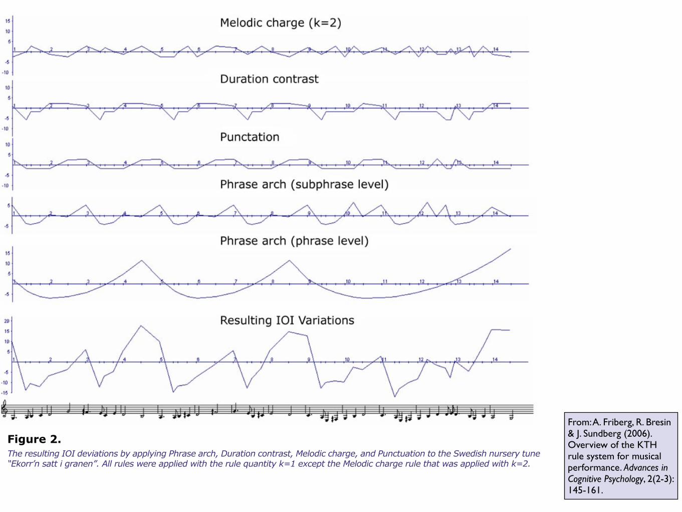
Figure 2.

The resulting IOI deviations by applying Phrase arch, Duration contrast, Melodic charge, and Punctuation to the Swedish nursery tune “Ekorr’n satt i granen”. All rules were applied with the rule quantity k=1 except the Melodic charge rule that was applied with k=2.


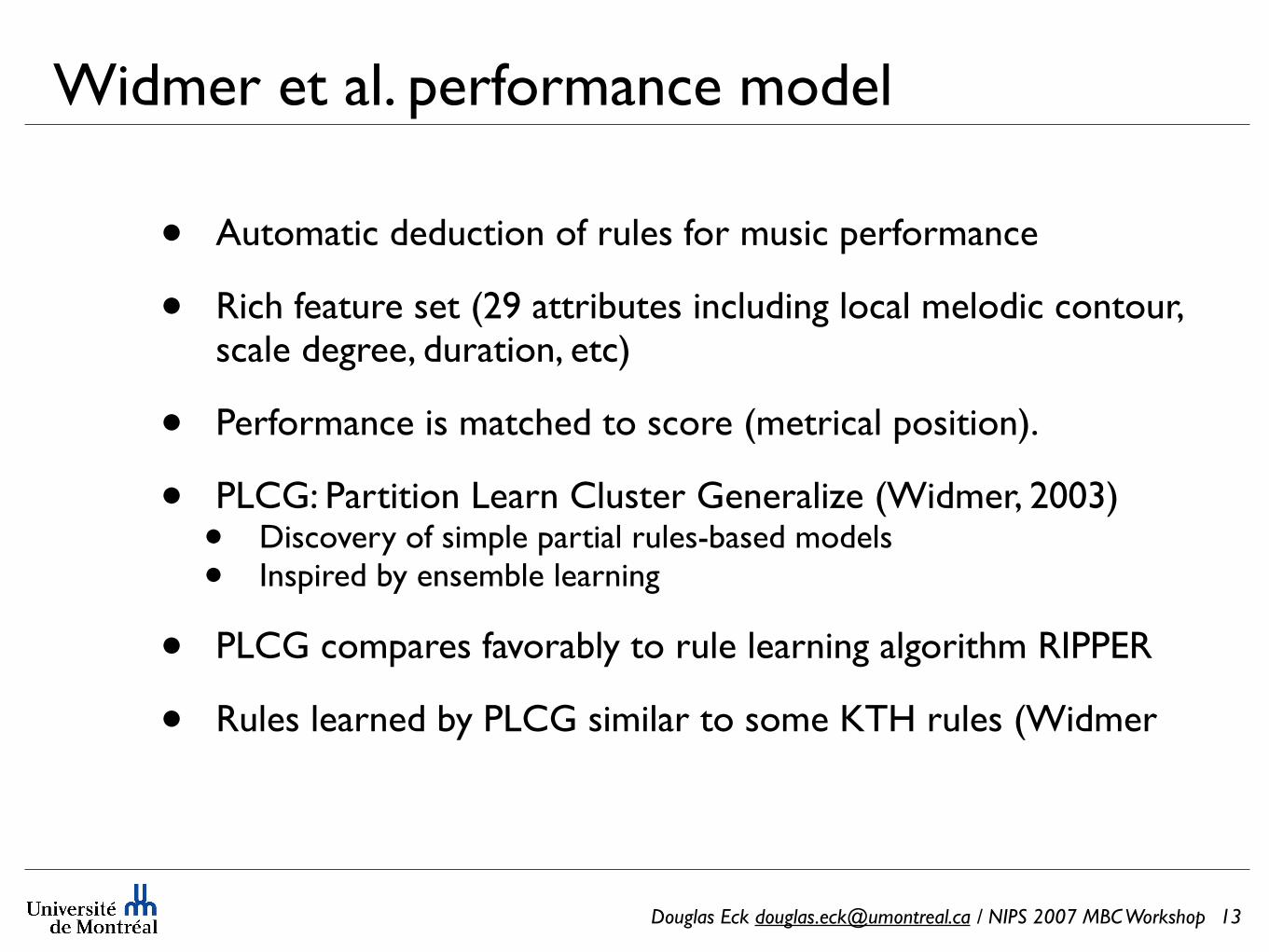
Widmer et al. performance model

• Automatic deduction of rules for music performance

• Rich feature set (29 attributes including local melodic contour, scale degree, duration, etc)

• Performance is matched to score (metrical position).

• PLCG: Partition Learn Cluster Generalize (Widmer, 2003)• Discovery of simple partial rules-based models• Inspired by ensemble learning

• PLCG compares favorably to rule learning algorithm RIPPER

• Rules learned by PLCG similar to some KTH rules (Widmer

13



140 G. Widmer / Artificial Intelligence 146 (2003) 129–148

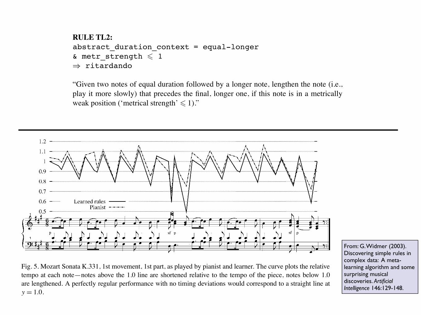
Fig. 5. Mozart Sonata K.331, 1st movement, 1st part, as played by pianist and learner. The curve plots the relative

tempo at each note—notes above the 1.0 line are shortened relative to the tempo of the piece, notes below 1.0

are lengthened. A perfectly regular performance with no timing deviations would correspond to a straight line at

y = 1.0.

simple rules (one for note lengthening (ritardando), one for shortening (accelerando)) that

produce the system’s timing curve.4

The next question concerns the generality of the discovered rules. How well do they

transfer to other pieces and other performers? To assess the degree of performer-specificity

of the rules, they were tested on performances of the same pieces, but by a different

artist. The test pieces in this case were the Mozart sonatas K.282, K283 (complete) and

K.279, K.280, K.281, K.284, and K.333 (second movements), performed by the renowned

conductor and pianist Philippe Entremont, again on a Bösendorfer SE290. The results are

given in Table 3.

Comparing this to Table 2, we find no significant degradation in coverage and precision

(except in category diminuendo). On the contrary, for some categories (ritardando,

crescendo, staccato) the coverage is higher than on the original training set. The

discriminative power of the rules —the precision—remains roughly at the same level. This

(surprising?) result testifies to the generality of the discovered principles; PLCG seems to

have successfully avoided overfitting the training data.

Another experiment tested the generality of the discovered rules with respect to musical

style. They were applied to pieces of a very different style (Romantic pianomusic), namely,

the Etude Op.10, No.3 in E major (first 20 bars) and the Ballade Op.38, F major (first 45

bars) by Frédéric Chopin, and the results were compared to performances of these pieces

by 22 Viennese pianists. The melodies of these 44 performances amount to 6,088 notes.

Table 4 gives the results.

This result is even more surprising. Diminuendo and legato turn out to be basically

unpredictable, and the rules for crescendo are rather imprecise. But the results for the

other classes are extremely good, better in fact than on the original (Mozart) data which

4 To be more precise: the rules predict whether a note should be lengthened or shortened; the precise numeric

amount of lengthening/shortening is predicted by a k-nearest-neighbor algorithm (with k = 3) that uses only

instances for prediction that are covered by the matching rule, as proposed in [26] and [27].

138 G. Widmer / Artificial Intelligence 146 (2003) 129–148

4. Musical discoveries made by PLCG

Let us first look at some of PLCG’s discoveries from a musical perspective. Section 5

below we will then take a more systematic experimental look at PLCG’s behaviour relative

to more ‘direct’ rule learning.

4.1. Performance principles discovered

When run on the complete Mozart performance data set (41,116 notes) for each of

the six target concepts defined above,3 PLCG (with parameter settings MPPLCG = .7,

MCPLCG = .02,MPRL = .9,MCRL = .01) selected a final set of 17 performance rules (from

a total of 383 specialized rules)—6 rules for tempo changes, 6 rules for local dynamics, and

5 rules for articulation. (Two rules were selected manually for musical interest, although

they did not quite reach the required coverage and precision, respectively.) Some of these

rules turn out to be discoveries of significant musicological interest. We lack the space to

list all of them here (see [32]). Let us illustrate the types of patterns found by looking at

just one of the learned rules:

RULE TL2:

abstract_duration_context = equal-longer

& metr_strength ! 1

! ritardando

“Given two notes of equal duration followed by a longer note, lengthen the note (i.e.,

play it more slowly) that precedes the final, longer one, if this note is in a metrically

weak position (‘metrical strength’ ! 1).”

This is an extremely simple principle that turns out to be surprisingly general and

precise: rule TL2 correctly predicts 1,894 cases of local note lengthening, which is 14.12%

of all the instances of significant lengthening observed in the training data. The number of

incorrect predictions is 588 (2.86% of all the counterexamples). Together with a second,

similar rule relating to the same type of phenomenon, TL2 covers 2,964 of the positive

examples of note lengthening in our performance data set, which is more than one fifth

(22.11%)! It is highly remarkable that one simple principle like this is sufficient to predict

such a large proportion of observed note lengthenings in a complex corpus such as Mozart

sonatas. This is a truly novel (and surprising) discovery; none of the existing theories of

expressive performance were aware of this simple pattern.

3 In this experiment, the data were not split into subsets randomly; rather, 10 subsets were created according

to global tempo (fast or slow) and time signature (3/4, 4/4, etc.) of the sonata sections the notes belonged to. We

chose these two dimensions for splitting because it is known (and has been shown experimentally [28]) that global

tempo and time signature strongly affect expressive performance patterns. As a result, we can expect models that

tightly fit (overfit?) these data partitions to be quite different, and diversity should be beneficial to an ensemble

method like PLCG.

From: G. Widmer (2003). Discovering simple rules in complex data: A meta-learning algorithm and some surprising musical discoveries. Artificial Intelligence 146:129-148.


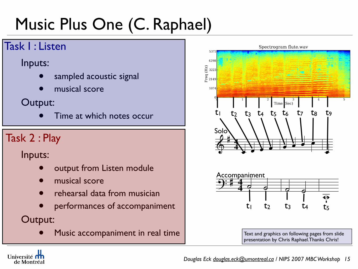
Music Plus One (C. Raphael)

Inputs:

• sampled acoustic signal

• musical score

Output:

• Time at which notes occur

Inputs:

• output from Listen module

• musical score

• rehearsal data from musician

• performances of accompaniment

Output:

• Music accompaniment in real time

15

Task I : Listen

Task 2 : Play

t1 t2 t3 t4 t5 t6 t7 t8 t9

44

Text and graphics on following pages from slide presentation by Chris Raphael.Thanks Chris!

44

t1 t2 t3 t4 t5

Solo

Accompaniment



0

5

10

15

20

25

30

35

0 1 2 3 4 5 6 7 8

seconds

measures

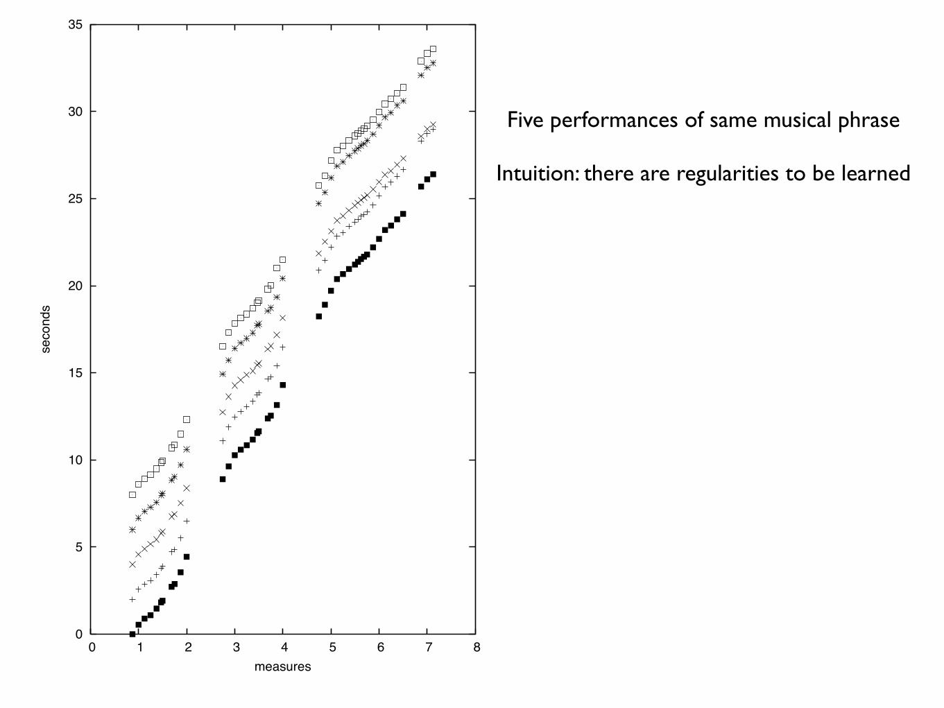
Five performances of same musical phrase

Intuition: there are regularities to be learned


Composite

Accomp

Listen

Update

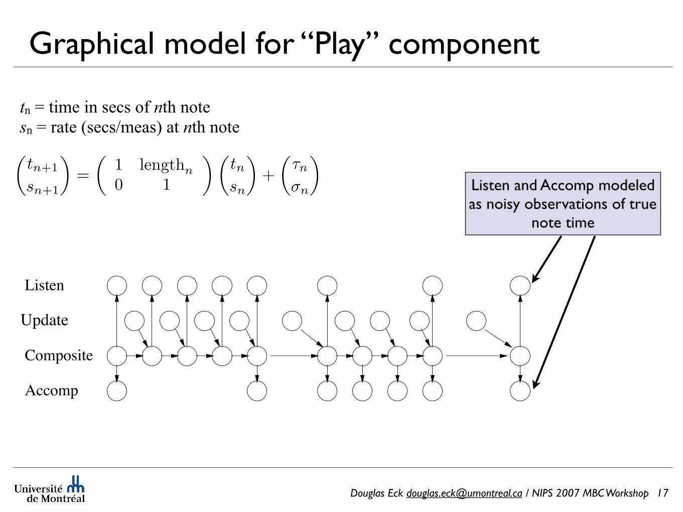
tn = time in secs of nth notesn = rate (secs/meas) at nth note

!tn+1

sn+1

"=

!1 lengthn

0 1

" !tnsn

"+

!!n

"n

"

Listen and Accomp modeled as noisy observations of true

note time

Graphical model for “Play” component

17




Composite

Accomp

Listen

Update

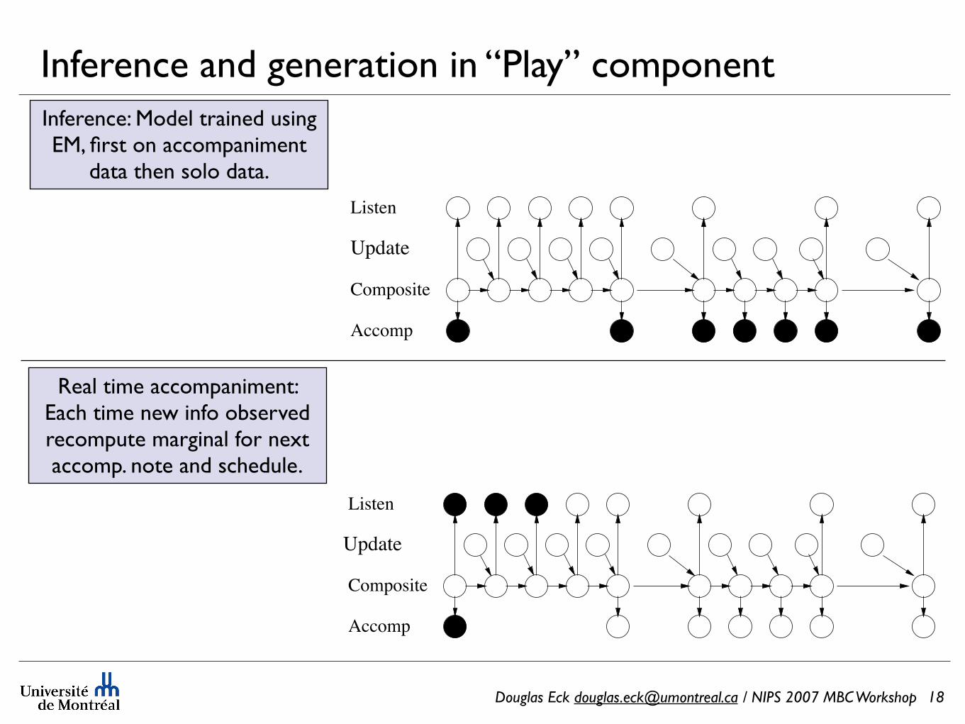
Inference: Model trained using EM, first on accompaniment

data then solo data.

Inference and generation in “Play” component

18

Real time accompaniment: Each time new info observed recompute marginal for next accomp. note and schedule.

Composite

Accomp

Listen

Update

Process frame Play pending note

Signal handler

reschedule next unplayed noteIf solo note detected, Schedule next unplayed note




KCCA (Dorard, Hardoon & Shawe-Taylor)

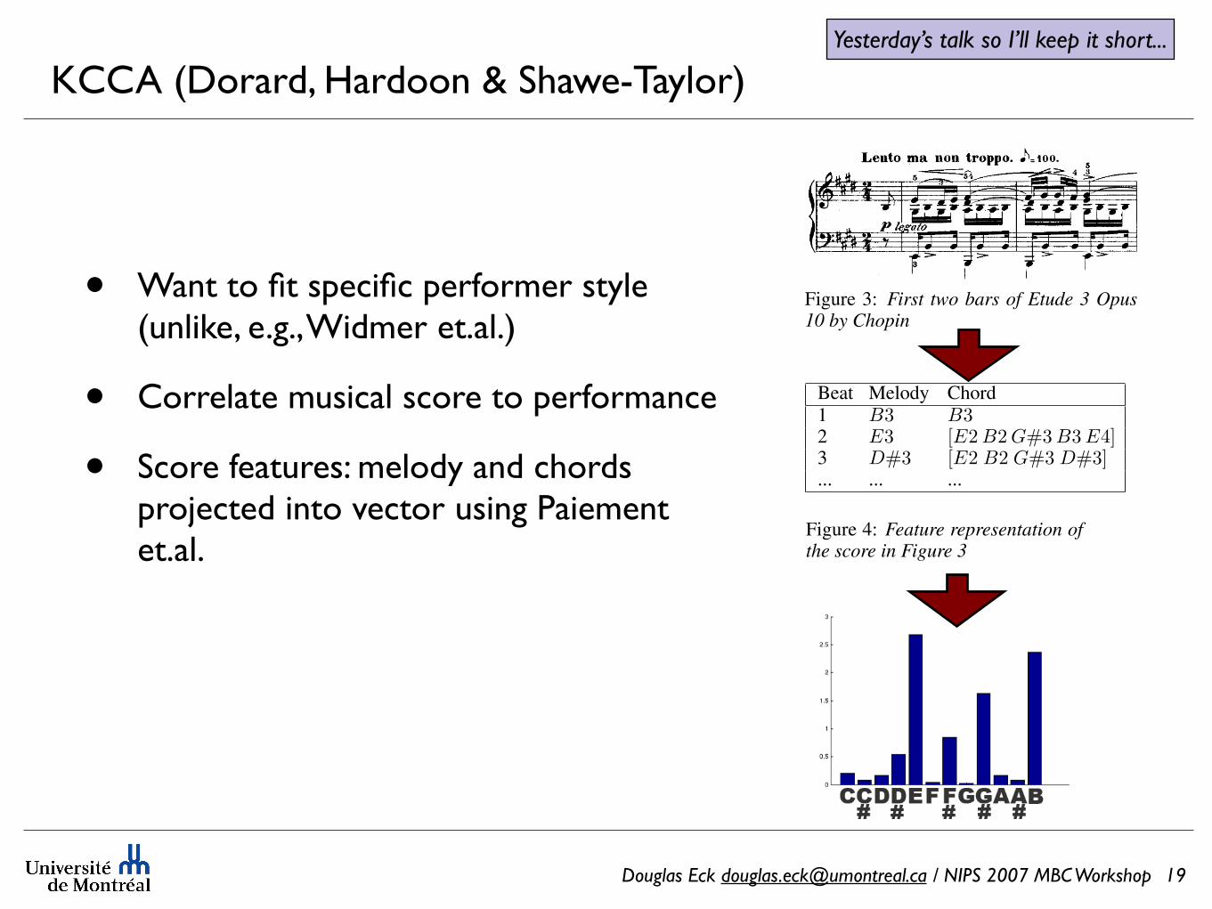
• Want to fit specific performer style (unlike, e.g., Widmer et.al.)

• Correlate musical score to performance

• Score features: melody and chordsprojected into vector using Paiement et.al.

19

Yesterday’s talk so I’ll keep it short...

In our approach we confine ourselves to expressive music with continuous upper partmelody and accompaniment2, as we believe this type of music to be simpler to analysefor the purpose of performance. It may be interesting to consider scores that make use ofrubato as this implies important variations in tempo, at the discretion of the performer. Itwould make it easier to see whether our technique yields good results. ‘Etude 3 Opus 10’by Chopin (Figure 3) is a prime example of the kind of music we consider as it has all thecharacteristics mentioned above.

For such music we can easily extract the melody, and then the harmonies: we assign to eachnote of the melody the chord made up of the notes played in the accompaniment while thenote of the melody stays on. Thus we create a sequence of (note, chord) pairs occurringone after another, which we call ‘feature representation’.This is musically relevant as it captures both the ’vertical’ and the ’horizontal’ dimensionsof music. Figure 4 shows an example of the extracted feature representation of a musicalscore. We will use our learning algorithms with these feature representations instead ofscores in the note matrix format. The principal advantage of the feature representation isthat, unlike the score, no event can occur while another event is already on.

Figure 3: First two bars of Etude 3 Opus10 by Chopin

Beat Melody Chord1 B3 B32 E3 [E2 B2 G#3 B3 E4]3 D#3 [E2 B2 G#3 D#3]... ... ...

Figure 4: Feature representation ofthe score in Figure 3

The audio recordings used initially are all chosen from the same performer, which style wetry to learn, and there is only one recording per score. Hence, the data used in our systemis a paired data-set containing first, score feature representations and second, performanceworms. The system learns how a famous pianist performs by relating the worm to the struc-ture of the music as it is written on the score, and then perform new pieces of music usingthe learned style. We use KCCA to correlate the two views and to learn the common “se-mantic space” in which they are to be projected. When dealing with a new score, we seekto generate a worm sequence that maximises the similarity with the score in the commonsemantic space (i.e. the inner product in that space). The worm coordinates are then usedto set the timing of notes and their velocity, thus generating a performance – limited, sincethe attack of a key on the piano cannot be summarised with just one value for the velocity.

In order to apply KCCA to our data, we first need to design a kernel that applies to sec-tions of worm and a kernel that applies to sections of musical score, which we call ’MusicKernel’ and we present in this paper.

2 Music Kernel

We begin by introducing some notations that will be used throughout the paper. Let s1

denote a sequence of events in time (s1,j)j such that(j1 < j2)! (s1,j1 happens before s1,j2). (1)

Each event e is characterised by its position in time – also called “onset time” – and itsattributes that we assume to be vectors of real numbers. Events occur one after another,

2Continuous: no rests; Upper part: at any given time, the note with the highest pitch that can beheard is a note of the melody; Accompaniment: the notes which are not part of the melody and whichare used to create harmonies.

In our approach we confine ourselves to expressive music with continuous upper partmelody and accompaniment2, as we believe this type of music to be simpler to analysefor the purpose of performance. It may be interesting to consider scores that make use ofrubato as this implies important variations in tempo, at the discretion of the performer. Itwould make it easier to see whether our technique yields good results. ‘Etude 3 Opus 10’by Chopin (Figure 3) is a prime example of the kind of music we consider as it has all thecharacteristics mentioned above.

For such music we can easily extract the melody, and then the harmonies: we assign to eachnote of the melody the chord made up of the notes played in the accompaniment while thenote of the melody stays on. Thus we create a sequence of (note, chord) pairs occurringone after another, which we call ‘feature representation’.This is musically relevant as it captures both the ’vertical’ and the ’horizontal’ dimensionsof music. Figure 4 shows an example of the extracted feature representation of a musicalscore. We will use our learning algorithms with these feature representations instead ofscores in the note matrix format. The principal advantage of the feature representation isthat, unlike the score, no event can occur while another event is already on.

Figure 3: First two bars of Etude 3 Opus10 by Chopin

Beat Melody Chord1 B3 B32 E3 [E2 B2 G#3 B3 E4]3 D#3 [E2 B2 G#3 D#3]... ... ...

Figure 4: Feature representation ofthe score in Figure 3

The audio recordings used initially are all chosen from the same performer, which style wetry to learn, and there is only one recording per score. Hence, the data used in our systemis a paired data-set containing first, score feature representations and second, performanceworms. The system learns how a famous pianist performs by relating the worm to the struc-ture of the music as it is written on the score, and then perform new pieces of music usingthe learned style. We use KCCA to correlate the two views and to learn the common “se-mantic space” in which they are to be projected. When dealing with a new score, we seekto generate a worm sequence that maximises the similarity with the score in the commonsemantic space (i.e. the inner product in that space). The worm coordinates are then usedto set the timing of notes and their velocity, thus generating a performance – limited, sincethe attack of a key on the piano cannot be summarised with just one value for the velocity.

In order to apply KCCA to our data, we first need to design a kernel that applies to sec-tions of worm and a kernel that applies to sections of musical score, which we call ’MusicKernel’ and we present in this paper.

2 Music Kernel

We begin by introducing some notations that will be used throughout the paper. Let s1

denote a sequence of events in time (s1,j)j such that(j1 < j2)! (s1,j1 happens before s1,j2). (1)

Each event e is characterised by its position in time – also called “onset time” – and itsattributes that we assume to be vectors of real numbers. Events occur one after another,

2Continuous: no rests; Upper part: at any given time, the note with the highest pitch that can beheard is a note of the melody; Accompaniment: the notes which are not part of the melody and whichare used to create harmonies.

2.2 Events of different durations

It does not make much sense to compare events from s1 and s2 when they do not havethe same durations, because events will not happen at the same times within the sequence.For this reason, we transform one of the two sequences to be compared, say s1, so that itsevents happen at the exact same times in the sequence as those of s2, i.e. they have samedurations. We call such an operation a ‘projection’ and denote the resulting sequence bys(1!2).Figure 5 shows the behaviour of the projection algorithm on two examples. Each event isa rectangle, time is represented on a horizontal axis, and the attributes of the events arerepresented with the brightness of the rectangles’ colours.

Figure 5: Illustration of the projection algorithm

The sequence s(1!2) can be used instead of s1 in Equation 7 to compute a distance withs2. However, we may lose events of the original sequence when projecting it, as shown inFigure 5. In order not to lose the specificities of s1 and s2 when extending our distance tosequences of events of different durations, we define our new distance to be

dj0(s1, s2) =!

dj0(s1, s(2!1))2 + dj0(s(1!2), s2)2 (8)

Note that projection also makes a certain error since the durations pattern of s(1!2) is thesame as the one of s2, which is likely to be different from the durations pattern of s1.A measure of that error, e1!2, can be given by comparing the duration of each events(1!2),j with the duration of the event e chosen in s1 it originates from. Errors e1!2

and e2!1 can then both be incorporated into the new distance dj0 defined in Equation 8.

2.3 Application to scores

A score’s feature representation (Figure 4) is a time sequence in which events are (note,chord) pairs. The performance of the Music Kernel is dependent on the attributes of theseevents as the kernel is based on the distance between events which is based on a distancebetween the attributes. It is quite natural to consider the pitch, which is an integer, asthe attribute for a note. However it is not obvious which numerical attribute should beconsidered for a chord and could account its harmonic characteristics.

[2] developed a 12 dimensional representation of chordsbased on psycho-acoustic considerations. When a chordis played, not only the notes that make up the chord can beheard but also the harmonics of these notes. For instance,when a C3 is played, a G4 can be heard as a harmonic,with a lesser loudness. We first determine the loudnessesof all audible notes when the chord is sounded. Then,for each pitch-class (C, C#, D, ...) the loudnesses ofthe notes that belong to it are summed, this resulting in avector of 12 real values that we consider as the attribute

for the chord. It appears then that if two chords correspond to two different inversions ofthe same harmony, their attributes will be similar even though the chords could be made ofdifferent notes (e.g.: [E2 G#3 B3 E4] and [B2 E3 D2 G#2] for E major). The figureabove shows the attribute of the chord [E2 B2 G#3 B3 E4] as a histogram.




KCCA (Dorard, Hardoon & Shawe-Taylor)

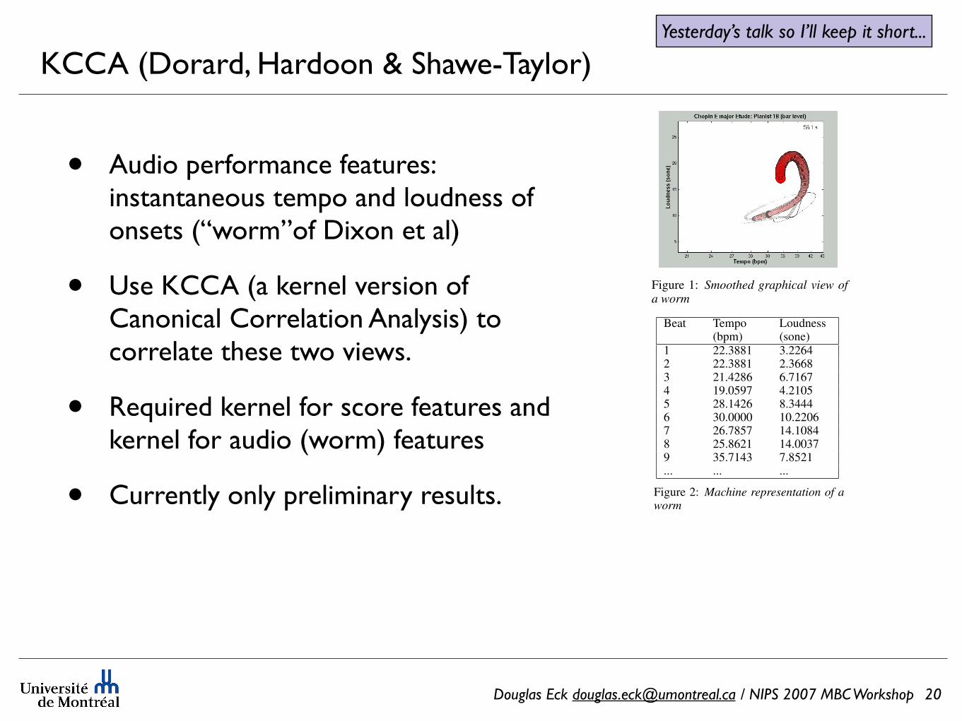
• Audio performance features: instantaneous tempo and loudness of onsets (“worm”of Dixon et al)

• Use KCCA (a kernel version of Canonical Correlation Analysis) to correlate these two views.

• Required kernel for score features and kernel for audio (worm) features

• Currently only preliminary results.

20

Yesterday’s talk so I’ll keep it short...

and then the machine would just know which notes to play and at which times. The restof the parameters of the performance would have to be initialised to default values andwouldn’t change. This would result in a mechanical and flat performance, allowing nodynamic nor time delay, and consequently lacking any emotion.One could argue that the musical score actually gives information on how to perform thepiece, but this information is only qualitative in nature (e.g. p, f, cresc., ral., acc.) andtherefore it cannot be readily implemented in the computer representation of the score.

The purpose of the present work is to use machine learning techniques in order to enablethe computer to perform a piece of music in the way a human would, and preferably in thestyle of one particular performer.Previous work such as [6] presented a technique for machine performance based on aninductive rule-learning algorithm. Thus, they were able to predict the dynamics of perfor-mances, as well as the changes of tempo. However their technique was restricted as they didnot consider the specificities of individual performers. They sought commonalities acrossall performers in the change in loudness and in tempo, to establish general rules. Besides,their method did not consider combined changes in loudness and tempo, and harmonieswere not considered in the analysis of scores.We seek here to achieve machine performance by correlating musical scores with perfor-mances of these scores. We assume that these two objects are two views of the samemusical semantic content S. Note that there is only one view of S in the form of a symbolicrepresentation (score) but there can be several views of S in the form of a performancetranscription (MIDI or audio recording for instance), as two different pianists will performdifferently the same piece of music or the same pianist could perform differently at differentmoments.

Although it should also be possible to use MIDI recordings as performance transcriptions(made by the Computer Grand Piano for example), we choose to work with audiorecordings which are more common especially when we look for recordings from famouspianists. From these audio recordings we extract performance worms as introduced by [3].Thereafter, a performance will be associated to its worm and we won’t have to consideraudio recordings again.Worms are sequences of 2 real values that give the evolution of tempo and loudness in timein the performance. Each (tempo, loudness) pair in the worm corresponds to a beat on thescore. Figure 1 shows a graphical view of a worm as a 2D trajectory on a graph. Pianists’specificity’s show with characteristic worm shapes, whereas a machine’s performanceworm would be immobile.

Figure 1: Smoothed graphical view ofa worm

Beat Tempo(bpm)

Loudness(sone)

1 22.3881 3.22642 22.3881 2.36683 21.4286 6.71674 19.0597 4.21055 28.1426 8.34446 30.0000 10.22067 26.7857 14.10848 25.8621 14.00379 35.7143 7.8521... ... ...

Figure 2: Machine representation of aworm

and then the machine would just know which notes to play and at which times. The restof the parameters of the performance would have to be initialised to default values andwouldn’t change. This would result in a mechanical and flat performance, allowing nodynamic nor time delay, and consequently lacking any emotion.One could argue that the musical score actually gives information on how to perform thepiece, but this information is only qualitative in nature (e.g. p, f, cresc., ral., acc.) andtherefore it cannot be readily implemented in the computer representation of the score.

The purpose of the present work is to use machine learning techniques in order to enablethe computer to perform a piece of music in the way a human would, and preferably in thestyle of one particular performer.Previous work such as [6] presented a technique for machine performance based on aninductive rule-learning algorithm. Thus, they were able to predict the dynamics of perfor-mances, as well as the changes of tempo. However their technique was restricted as they didnot consider the specificities of individual performers. They sought commonalities acrossall performers in the change in loudness and in tempo, to establish general rules. Besides,their method did not consider combined changes in loudness and tempo, and harmonieswere not considered in the analysis of scores.We seek here to achieve machine performance by correlating musical scores with perfor-mances of these scores. We assume that these two objects are two views of the samemusical semantic content S. Note that there is only one view of S in the form of a symbolicrepresentation (score) but there can be several views of S in the form of a performancetranscription (MIDI or audio recording for instance), as two different pianists will performdifferently the same piece of music or the same pianist could perform differently at differentmoments.

Although it should also be possible to use MIDI recordings as performance transcriptions(made by the Computer Grand Piano for example), we choose to work with audiorecordings which are more common especially when we look for recordings from famouspianists. From these audio recordings we extract performance worms as introduced by [3].Thereafter, a performance will be associated to its worm and we won’t have to consideraudio recordings again.Worms are sequences of 2 real values that give the evolution of tempo and loudness in timein the performance. Each (tempo, loudness) pair in the worm corresponds to a beat on thescore. Figure 1 shows a graphical view of a worm as a 2D trajectory on a graph. Pianists’specificity’s show with characteristic worm shapes, whereas a machine’s performanceworm would be immobile.

Figure 1: Smoothed graphical view ofa worm

Beat Tempo(bpm)

Loudness(sone)

1 22.3881 3.22642 22.3881 2.36683 21.4286 6.71674 19.0597 4.21055 28.1426 8.34446 30.0000 10.22067 26.7857 14.10848 25.8621 14.00379 35.7143 7.8521... ... ...

Figure 2: Machine representation of aworm




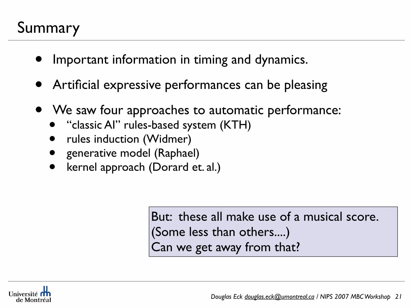
Summary

• Important information in timing and dynamics.

• Artificial expressive performances can be pleasing

• We saw four approaches to automatic performance:• “classic AI” rules-based system (KTH)• rules induction (Widmer)• generative model (Raphael)• kernel approach (Dorard et. al.)

21

But: these all make use of a musical score. (Some less than others....)Can we get away from that?




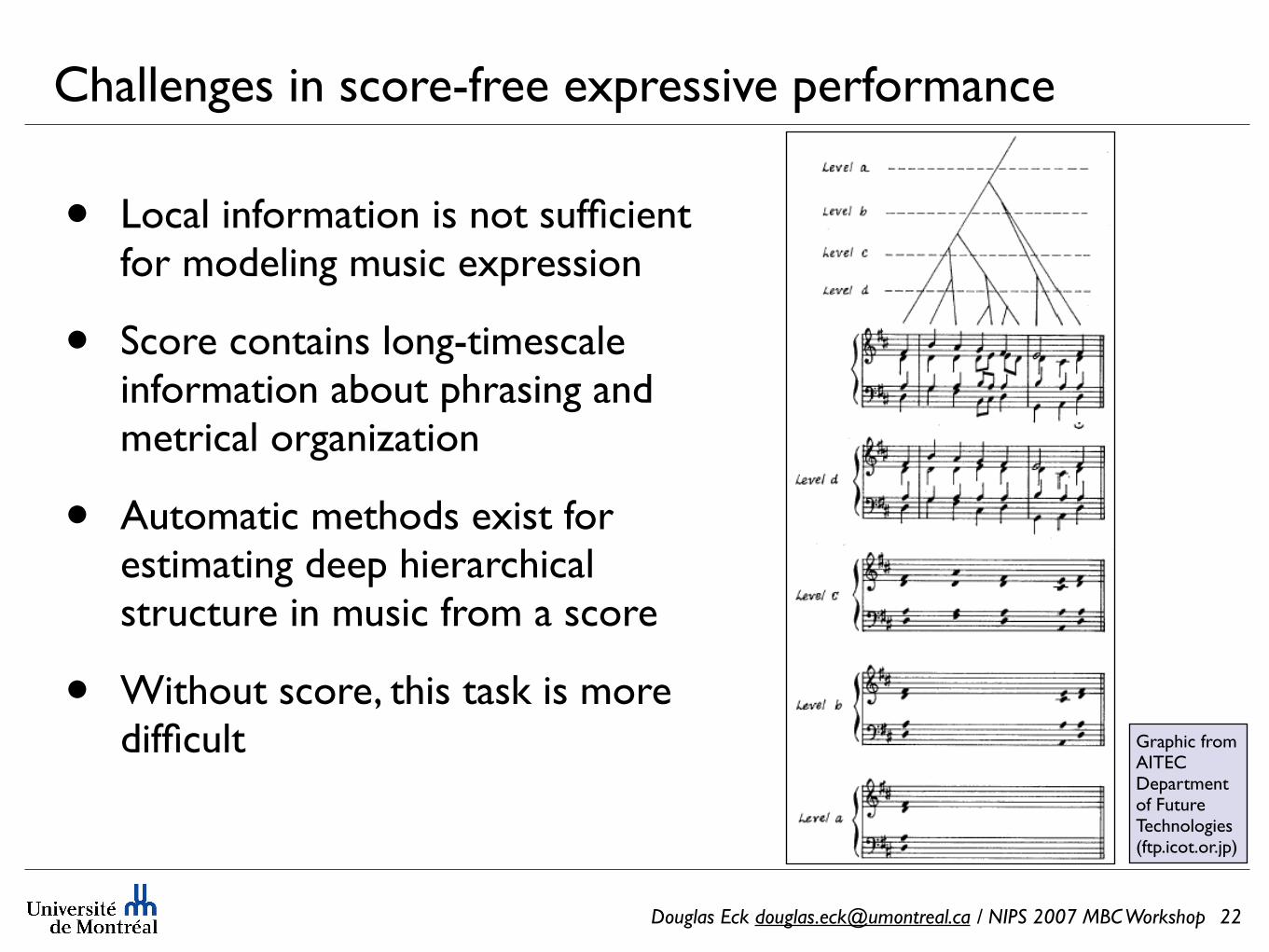
Challenges in score-free expressive performance

• Local information is not sufficient for modeling music expression

• Score contains long-timescale information about phrasing and metrical organization

• Automatic methods exist for estimating deep hierarchical structure in music from a score

• Without score, this task is more difficult

22

Graphic from AITEC Department of Future Technologies (ftp.icot.or.jp)




Incremental planning in sequence production 101

Event

Strength

Sx * Mx(i)

Metrically Strong

Current Event

Event

Strength

Sx* Mx(i)

Metrically Strong

Current Event

Metrically Weak

Current Event

Fast tempo

Metrically Weak

Current Event

Slow tempo*

*

Figure 7.

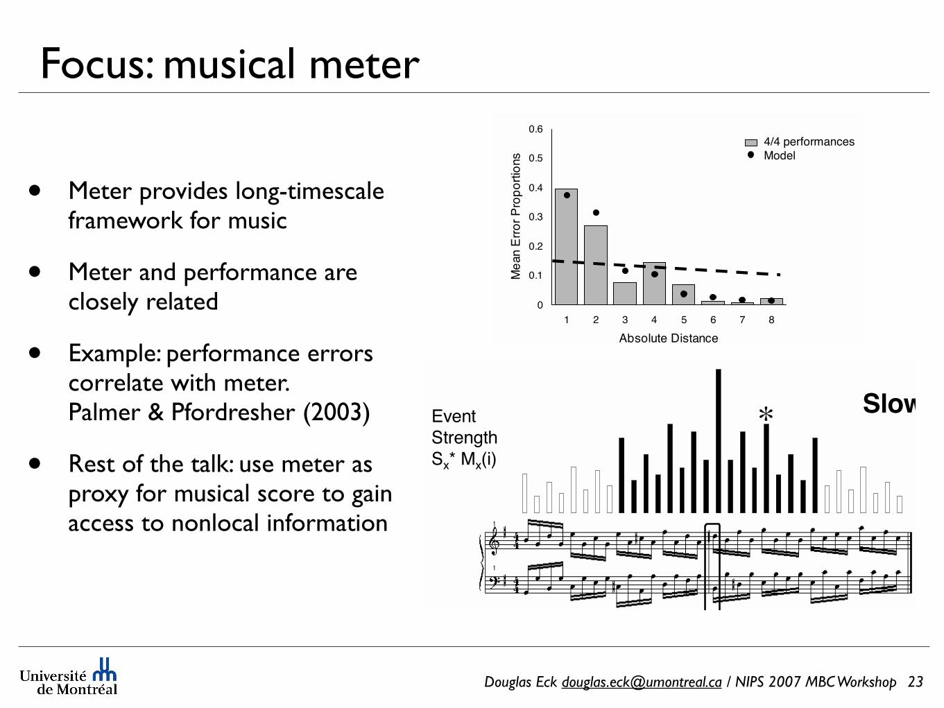
Focus: musical meter

• Meter provides long-timescale framework for music

• Meter and performance are closely related

• Example: performance errors correlate with meter. Palmer & Pfordresher (2003)

• Rest of the talk: use meter as proxy for musical score to gain access to nonlocal information

23

Incremental planning in sequence production 109

0

0.1

0.2

0.3

0.4

0.5

0.6

1 2 3 4 5 6 7 8

Absolute Distance

Me

an E

rro

r P

rop

ort

ions

0

0.1

0.2

0.3

0.4

0.5

0.6

1 2 3 4 5 6

Absolute Distance

Me

an E

rro

r P

rop

ort

ions

X X

X X X X

X X X X X X X

4/4 performances

Model

3/8 performances

Model

3

2

1

1

2

3

Figure 15.


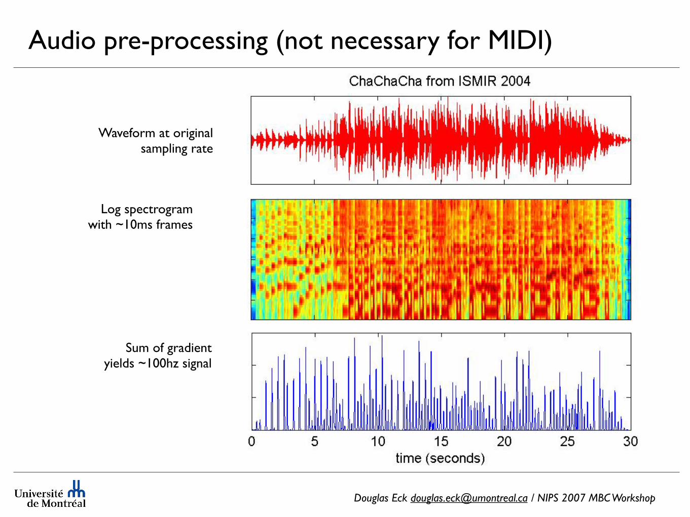
Waveform at original sampling rate

Log spectrogram with ~10ms frames

Sum of gradient yields ~100hz signal

Audio pre-processing (not necessary for MIDI)




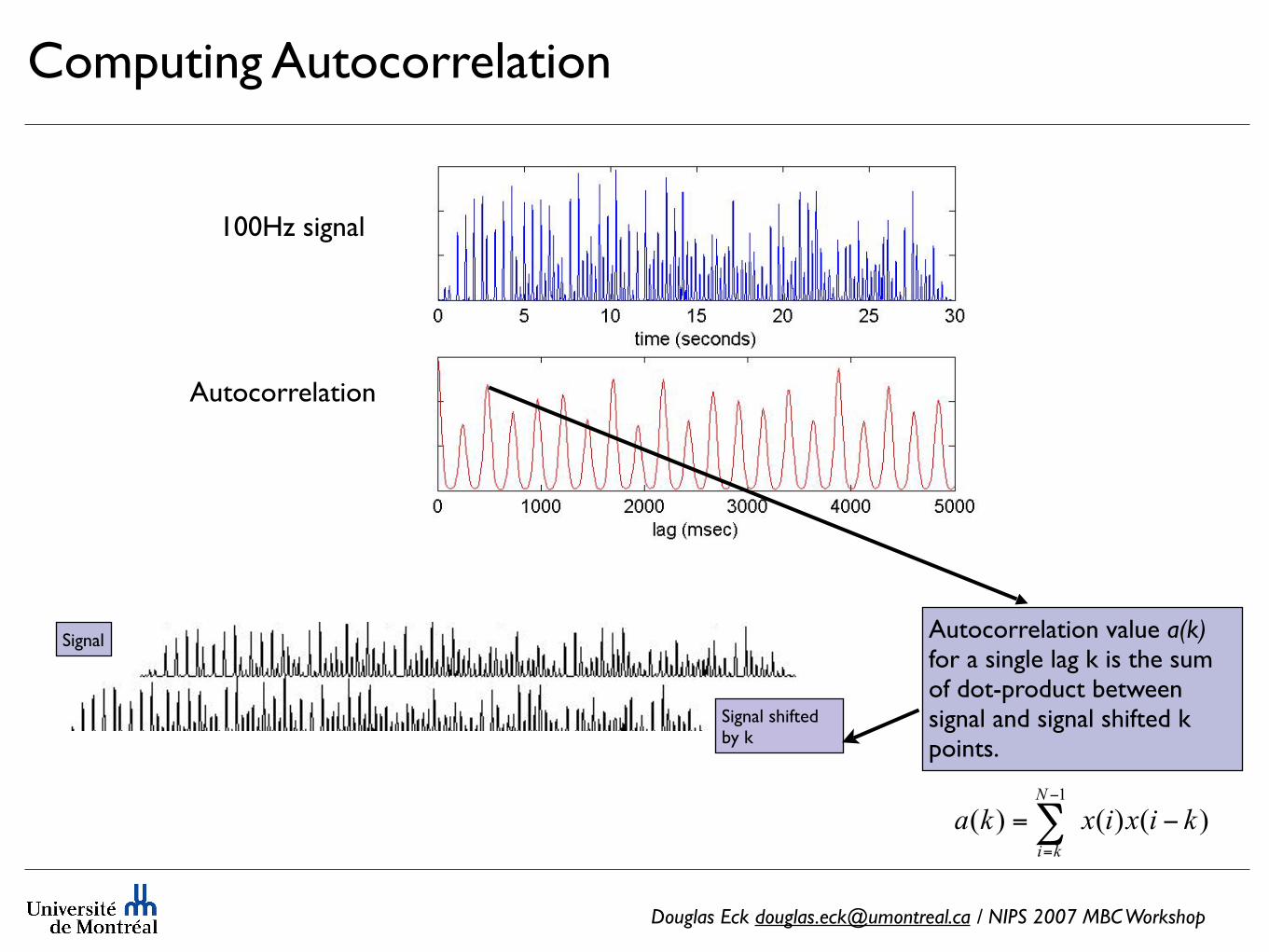
Autocorrelation value a(k)for a single lag k is the sum of dot-product between signal and signal shifted k points.

Signal

Signal shifted by k

Autocorrelation

100Hz signal

Computing Autocorrelation




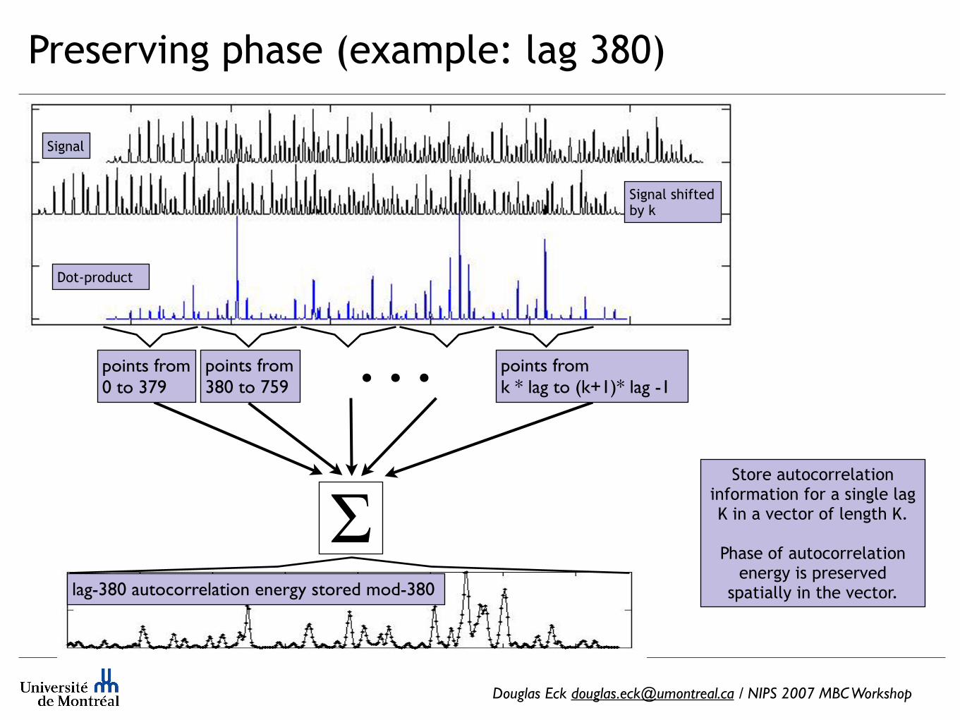
Store autocorrelation information for a single lag K in a vector of length K.

Phase of autocorrelation energy is preserved

spatially in the vector.

points from 0 to 379

points from 380 to 759

Preserving phase (example: lag 380)

points from k * lag to (k+1)* lag -1

. . .

Signal

Signal shifted by k

Dot-product

Σlag-380 autocorrelation energy stored mod-380




lag

(ms)

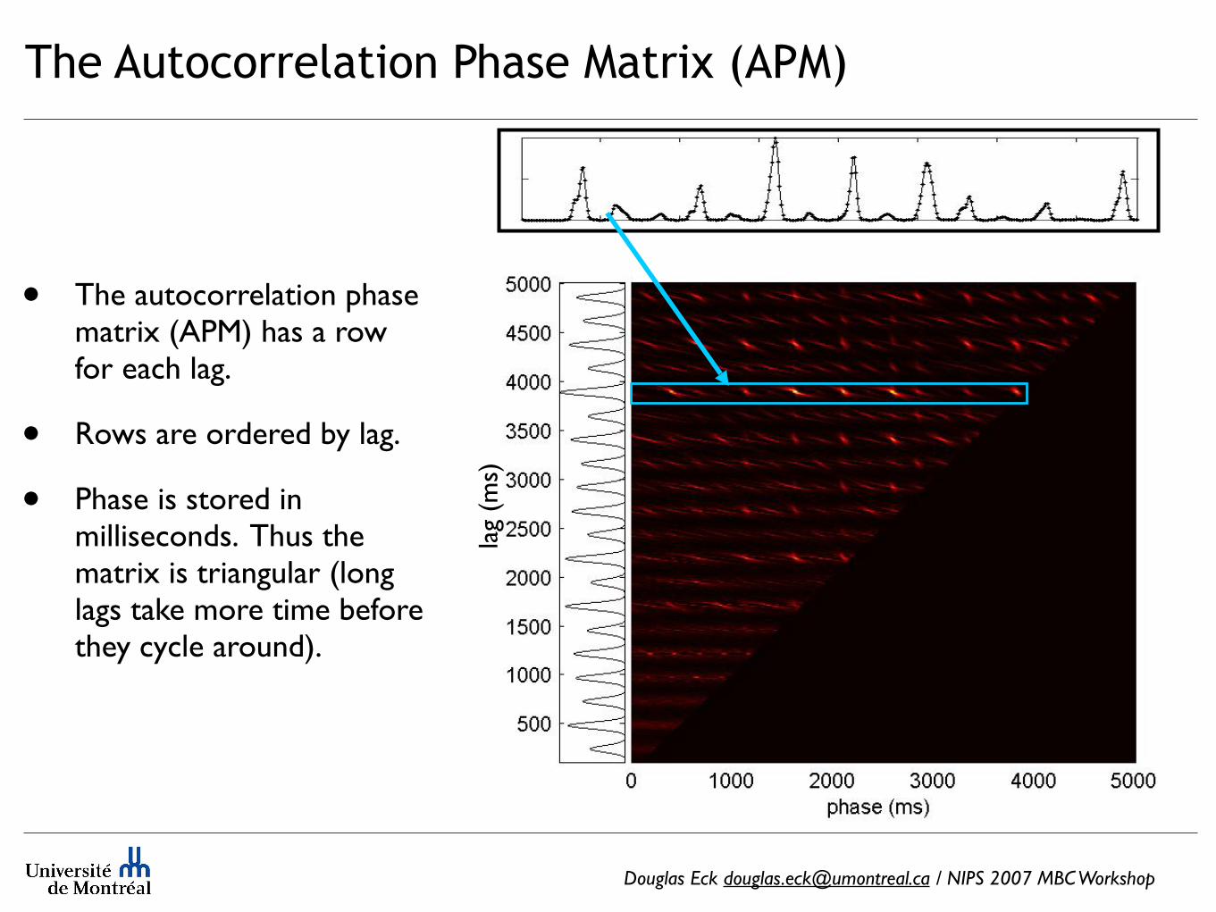
The Autocorrelation Phase Matrix (APM)

• The autocorrelation phase matrix (APM) has a row for each lag.

• Rows are ordered by lag.

• Phase is stored in milliseconds. Thus the matrix is triangular (long lags take more time before they cycle around).




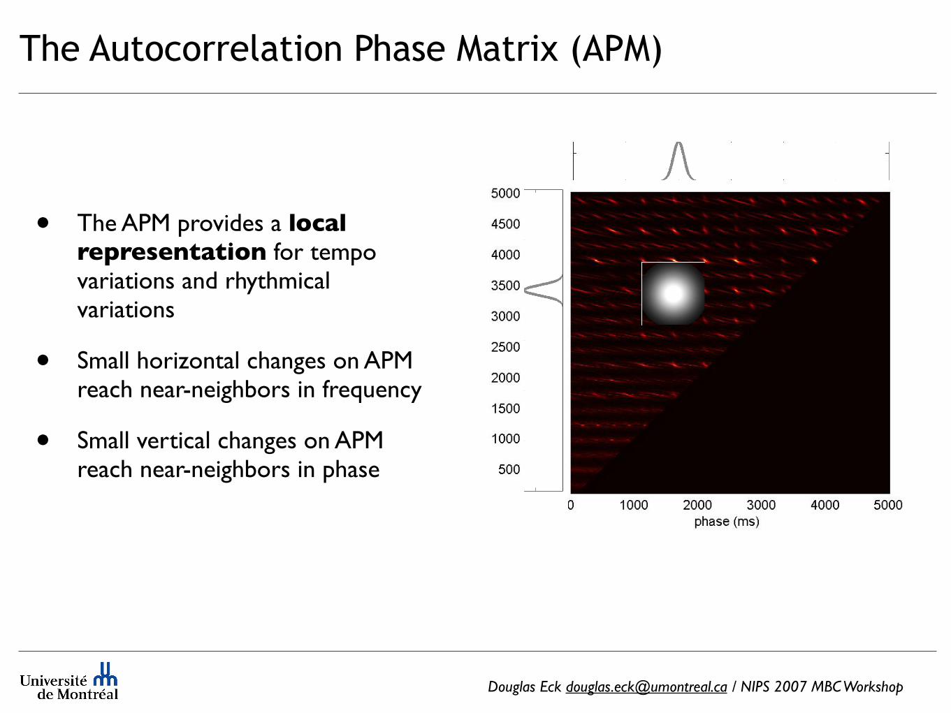
The Autocorrelation Phase Matrix (APM)

• The APM provides a local representation for tempo variations and rhythmical variations

• Small horizontal changes on APM reach near-neighbors in frequency

• Small vertical changes on APM reach near-neighbors in phase


lag

(ms)

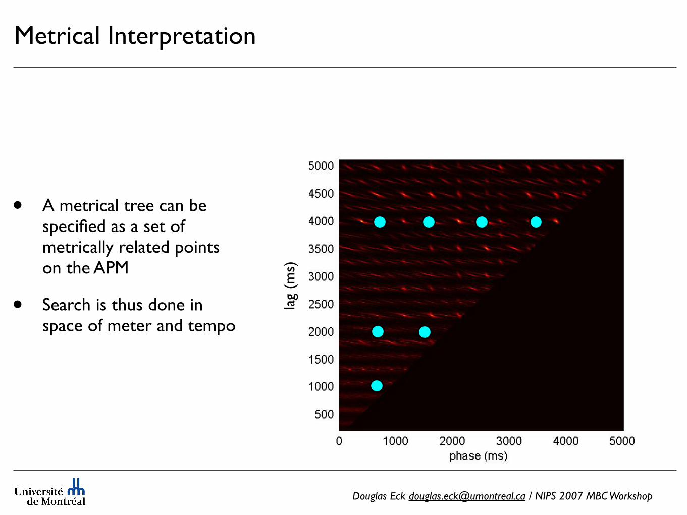
Metrical Interpretation

• A metrical tree can be specified as a set of metrically related points on the APM

• Search is thus done in space of meter and tempo




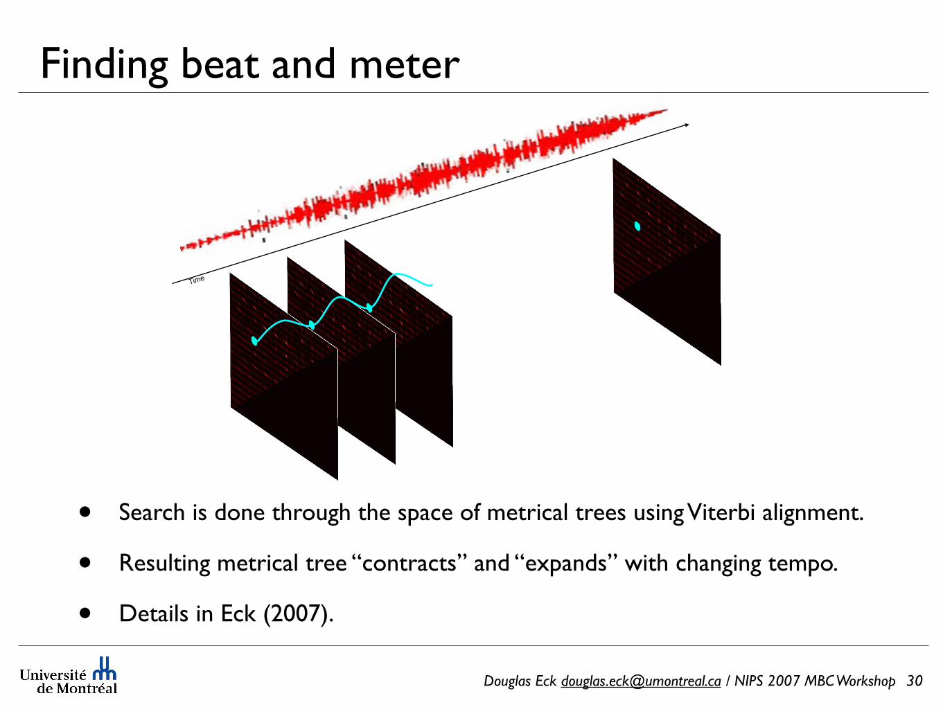
Finding beat and meter

• Search is done through the space of metrical trees using Viterbi alignment.

• Resulting metrical tree “contracts” and “expands” with changing tempo.

• Details in Eck (2007).

30

Time




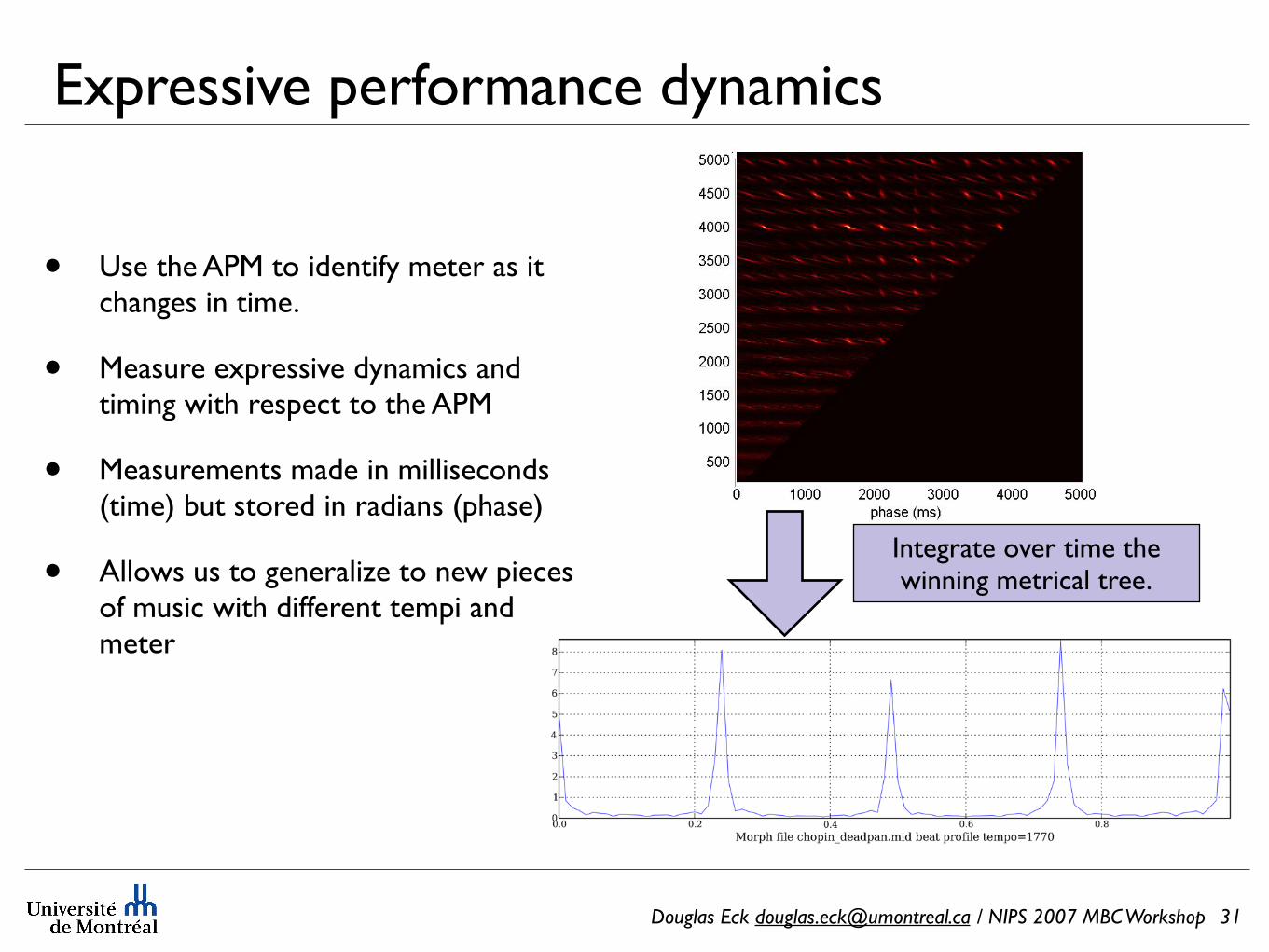
Expressive performance dynamics

• Use the APM to identify meter as it changes in time.

• Measure expressive dynamics and timing with respect to the APM

• Measurements made in milliseconds (time) but stored in radians (phase)

• Allows us to generalize to new pieces of music with different tempi and meter

31

Integrate over time the winning metrical tree.




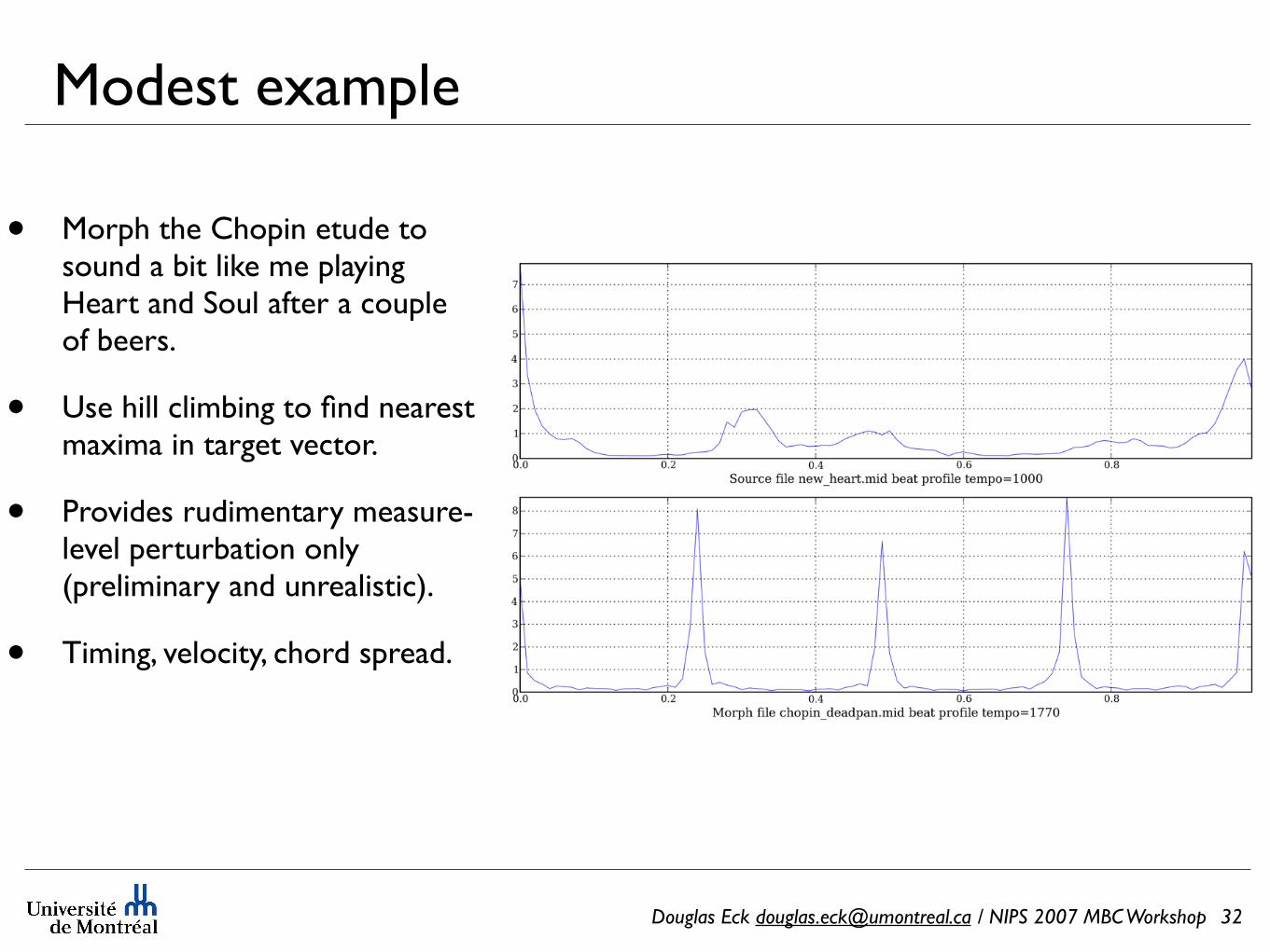
Modest example

• Morph the Chopin etude to sound a bit like me playing Heart and Soul after a couple of beers.

• Use hill climbing to find nearest maxima in target vector.

• Provides rudimentary measure-level perturbation only (preliminary and unrealistic).

• Timing, velocity, chord spread.

32




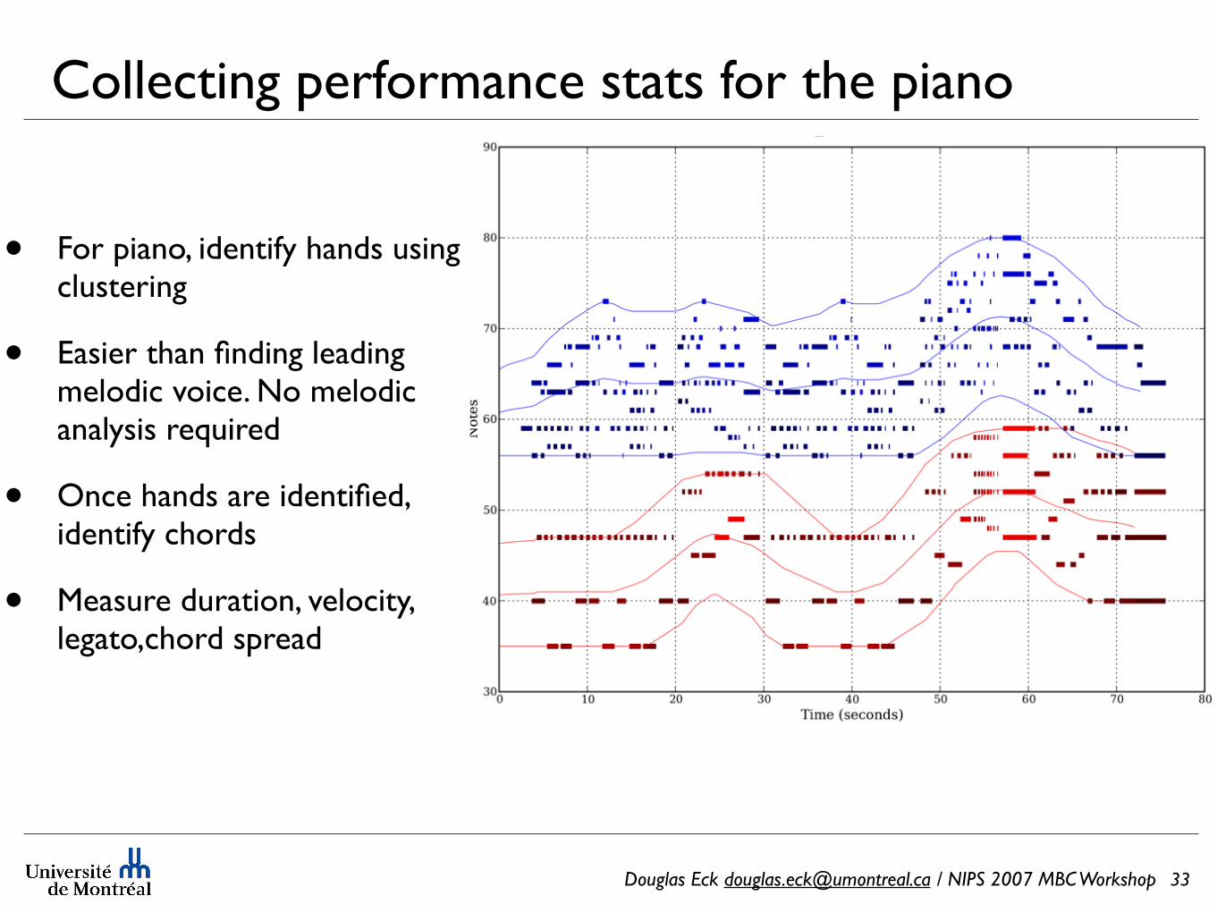
Collecting performance stats for the piano

• For piano, identify hands using clustering

• Easier than finding leading melodic voice. No melodic analysis required

• Once hands are identified, identify chords

• Measure duration, velocity, legato,chord spread

33




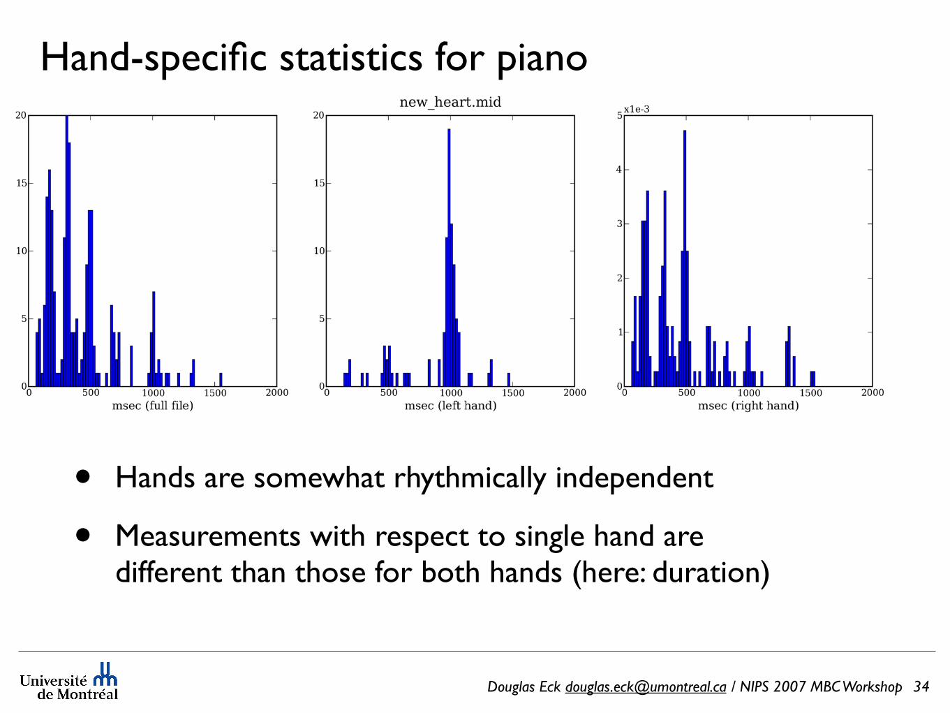
Hand-specific statistics for piano

• Hands are somewhat rhythmically independent

• Measurements with respect to single hand are different than those for both hands (here: duration)

34




Conclusions

• Expressive timing and dynamics are important part of music

• Short overview of approaches

• Discussed task of score-free expressive performance

• Suggest using metrical structure as proxy for musical score

• Related this to APM model

• Future work:

• There remains more future work than completed work!• So this list would be too long....• Thank you for your patience.

35




Bibliography

• B. Repp. (1990). Patterns of expressive timing in performances of a Beethoven minuet by nineteen famous pianists. Journal of the Acoustical Society of America, 88: 622-641.

• B. Repp. (1997). The aesthetic quality of a quantitatively average music performance: Two preliminary experiments. Music Perception, 14: 419-444.

• A. Friberg, R. Bresin & J. Sundberg (2006). Overview of the KTH rule system for musical performance. Advances in Cognitive Psychology, 2(2-3):145-161.

• G. Widmer (2003). Discovering simple rules in complex data: A meta-learning algorithm and some surprising musical discoveries. Artificial Intelligence 146:129-148.

• C. Raphael (2004). A Bayesian Network for Real-Time Musical Accompaniment, Neural Information Processing Systems (NIPS) 14.

• L. Dorard, D. Hardoon & J. Shawe-Taylor (2007). Can Style be Learned? A Machine Learning Approach Towards ‘Performing’ as Famous Pianists. NIPS Music Brain Cognition Workshop, Whistler.

• J.F. Paiement, D. Eck, S. Bengio & D. Barber (2005). A graphical model for chord progressions embedded in a psychoacoustic space. In Proceedings of the 22nd International Conference on Machine Learning (ICML), Bonn, Germany.

• S. Dixon, W. Goebl & G. Widmer (2002). The performance worm: Real time visualisation of expression based on Langner’s tempo-loudness animation. In Proceedings of the International Computer Music Conference (ICMC).

• C. Palmer & P. Pfordresher (2003). Incremental planning in sequence production. Psychological Review 110:683-712.

• D. Eck. (2007). Beat tracking using an autocorrelation phase matrix. In Proceedings of the 2007 International Conference on Acoustics, Speech and Signal Processing (ICASSP), 1313-1316.

36




Following are deleted slides

37




Deadpan (no expressive timing or dynamics)

Human performance (Recorded on Boesendorfer ZEUS)

Differences limited to:•timing (onset, length)•velocity (seen as red)•pedaling (blue shading)

Flat timingFlat velocity

Expressive timingFlat velocity

Expressive timingExpressive velocity


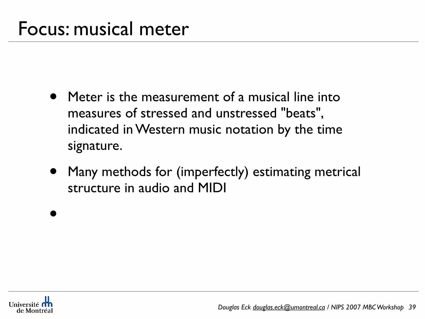
Focus: musical meter

• Meter is the measurement of a musical line into measures of stressed and unstressed "beats", indicated in Western music notation by the time signature.

• Many methods for (imperfectly) estimating metrical structure in audio and MIDI

•

39



measuring & modeling musical expressionpift6080/h08/documents/papers/eck... · 2008-12-04 ·...

Documents