measuring climatic impacts on energy consumption: a review...
TRANSCRIPT
Measuring Climatic Impacts on Energy Consumption:A Review of the Empirical Literature
Maximilian Auffhammer and Erin T. Mansur∗
April 25, 2014
Abstract
This paper reviews the literature on the relationship between climate and the energysector. In particular, we primarily discuss empirical papers published in peer-reviewedeconomics journals focusing on how climate affects energy expenditures and consump-tion. Climate will affect energy consumption by changing how consumers respond toshort run weather shocks (the intensive margin) as well has how people will adapt inthe long run (the extensive margin). Along the intensive margin, further research thatuses household and firm-level panel data of energy consumption may help identify howenergy consumers around the world respond to weather shocks. Research on technol-ogy adoption, e.g. air conditioners, will further our understanding of the extensivemargin adjustments and their costs. We also note that most of the literature focuseson the residential sector. Similar studies are urgently needed for the industrial andcommercial sectors.
JEL Codes: Q41, Q54
∗Auffhammer : UC Berkeley and NBER. 207 Giannini Hall, Berkeley, CA 94720, [email protected]; Mansur : Dartmouth College and NBER. Department of Economics, 6106 RockefellerHall, Hanover, NH 03755, [email protected]. We thank Dave Rapson for comments. Auffhammerthanks the Environmental Protection Agency for support under subcontract Q000-1C-1697. All remainingerrors are ours.
1 Introduction
This paper reviews the literature on the relationship between climate and the energy sector.
The energy climate relationship is interesting as it is a great example of a feedback effect. The
causal link from emissions due to the combustion of fossil fuels to deliver energy services to
climate change is well established. However, hotter summers and warmer winters will change
energy consumption and production patterns. A similar feedback mechanism is hypothesized
in land use (Pielke et al., 2002). There are several ways in which climate may affect energy
consumption. In the residential, commercial and industrial sectors one would, in a warmer
world, expect higher cooling demand, which would lead to increased electricity consumption.
On the other hand, fewer cold winter days would result in decreased heating demand, which
would drive down natural gas, oil and electricity demand. These are all demand side effects.
On the supply side, one would expect increased use of natural gas on hot days, as some
power plants become less efficient as well as higher natural gas consumption for generation
due to higher electricity demand. During the winter, there might be a decrease in natural
gas demand for generation due to lower electricity demand.
In this paper we survey the literature containing empirical papers published in peer-
reviewed economics journals focusing on how climate, which is generally defined as a long
run average of weather, affects energy expenditures and consumption. Most of the studies
we found focus on electricity consumption in the residential sector. The coverage of the
commercial and industrial sectors as well as studies on other fuels is most sparse. For
example, we could not locate any empirical peer-reviewed economics papers on the effect of
climate on energy supply.
The empirical estimates of climate sensitivity of the energy sector are typically used to
predict the cost of climate change adaptation. Climate models predict a range of changes to
temperature, precipitation, and other climate measures. Most models predict a significant
increase in global average temperatures by the end of the current century for scenarios
close to a business as usual emissions path (IPCC SRES Scenario A1fi) or a slightly more
optimistic emissions path (A2). Auffhammer et al. (2013) provide a detailed discussion of
1
climate models and their use in the social sciences. Overall one expects that people heat less
and cool more. This change in behavior will have both an intensive and extensive margin
component.
With regards to the intensive margin, several papers examine the short run response to
weather shocks. A common finding in this literature is that usage patterns of existing capital,
such as air conditioners, changes in response to climate change. Over time, however, we
posit that people will respond to climatic change along extensive margins. They may change
purchasing decisions of appliances, switch fuel sources, and even building characteristics. In
general, economists know less about these extensive margin adjustments than the intensive
ones. While research shows that future generations will likely own more air conditioners, this
is due to both price and income effects (Wolfram et al., 2012). There is a nascent literature
examining the weather and climate response of air conditioner adoption (e.g. Auffhammer,
2012, 2014).
The questions that researchers will continue to face include: How will climate change
affect peoples’ energy expenditures, choice of fuel sources, and buildings? How will people
adapt to a new and continuously changing climate? What will be the transitional costs of
adapting? Much of the uncertainty over the energy costs associated with climate change
will inevitably depend on the future income distribution and technologies. Nonetheless,
economists have made some progress in studying two complementary issues: first, how energy
choices differ among households and firms located in different climates; and second, how
a given consumer responds to weather shocks. From a policy perspective, studies of the
intensive margin and extensive margin adjustments speak to different, yet relates, policy
measures. If one is interested in short run reductions of weather driven energy demand (e.g.
peak load) information campaigns, peak pricing and direct load control may be effective
ways to achieve reductions in consumption. If one is interested in controlling the extensive
margin adjustment, efficiency standards, rebates for efficient appliances and insulation may
be more effective. While we do not speak to policy in this paper directly, this is an interesting
dichotomy. Below, we review this literature, discuss where the literature could head, and
2
outline the policy implications.
To address this question, the ideal data set would provide information on how a given
household consumes energy in randomly assigned climates, all else equal. Unfortunately,
this perfect experiment is not feasible as people sort into their preferred climate. One could
imagine trying to identify how consumers adapt to climate three different ways. One is to
look at how a given household’s consumption changes when it relocates to a new climate.
For example, how do military families’ energy expenditures change when they are relocated
to a new climate? This approach raises identification concerns regarding the reason why
people move, and why they chose a new housing type. No paper has attempted to explicitly
deal with the sorting approach to our knowledge.
A second approach that some economists use is to look at the cross-sectional variation in
climate. Namely, if there are two seemingly identical households that are located in different
climatic zones, one can then look at how their energy choices differ and ask whether these
differences are correlated with climate differences. The main concern with this approach is
that estimates are subject to omitted variables bias: unobservable differences in households
may be correlated with climate. For example, Albouy et al. (2012) find northern households
to be less heat-tolerant than southern households. Another issue with looking at cross-
sectional data is that we do not get an appreciation of the transition costs of fully adapting
to a new climate.
The third approach uses panel (or simply time series) variation to examine how energy
consumption responds to weather shocks. Recent studies of this reduced-form, short run
response include Deschenes and Greenstone (2011) and Auffhammer and Aroonruengsawat
(2011, 2012b). These estimates could overstate the damages of climatic change since house-
holds can adapt to a gradually changing environment in ways that they would not adapt to
short-run weather shocks (Deschenes and Greenstone, 2011). On the other hand, these esti-
mates may understate the damages, as individuals may adapt along the extensive margins
by purchasing additional capital equipment in the long run, which they might not have done
in the time frame of the data.
3
The paper is structured as follows. Section 2 lays a theoretical foundation to understand
the aim of this literature. Section 3 reviews the literature on cross-sectional climatic evidence
and panel (or time series) evidence of weather shocks. In Section 4, we discuss the gaps in
the literature and where the literature may head. In particular, we examine the need to
incorporate the literature on technology adoption in the estimation of the energy effects of
climate adaptation. Finally, Section 5 offers concluding remarks on the state of the literature
and its policy implications.
2 Theory
Before examining specific papers in this literature, we provide a theoretical foundation to
understand why households may change energy expenditures in response to climate change.
Define the utility function for a household as follows:
U = U( ~E, ~D, Y ;F0(t)), (1)
where ~E is a vector of energy sources like electricity, oil, and natural gas. ~D is a vector of
durable goods that affect the marginal utility of energy use like refrigerators, air conditioners,
and insulation. The other variables are a composite good Y , or numeraire, and the current
distribution of (outdoor) temperature F0(t), or simply F0. We could broaden the definition
of F0 to include other climate variables that would affect households’ purchasing decisions.
For example, humidity may affect a household’s choice of air conditioning (part of ~D), which
has implications for its choices of energy sources and other durables.
A household will maximize utility by choosing ~E, ~D, and Y , subject to income (I), energy
prices (~PE), durables prices (~PD), the price of the composite good (normalized to one), and
its expectation of distribution of temperatures, F0:
max~E, ~D,Y
U(.;F0) s.t. ~P ′E ~E + ~P ′D~D + Y ≤ I, (2)
where we denote the choices that maximize utility given the current climate as ~E∗(F0),
~D∗(F0), and Y ∗(F0).
4
A household derives utility from ~E∗(F0) and ~D∗(F0), in part, because the household
can control the interior temperature, tin. The energy needed to attain tin depends on the
absolute difference between tin and the exterior temperature t, given the set of durables:
~E = ~E(|tin − t|; ~D).
Climate change, by definition, alters the probability f(t) of experiencing temperature t
on a given day. As a result, the distribution will change (gradually) from F0(t) to Fτ (t), or
Fτ . In response, a household may choose to allow the interior temperature to vary with t.
However, if it does maintain a constant interior temperature, then the change in expenditures
measures the welfare effects of climate change (∆W ):
∆W = ~P ′E ·(~E∗(Fτ )− ~E∗(F0)
)+ ~P ′D
(~D∗(Fτ )− ~D∗(F0)
). (3)
There are several caveats to consider. First, energy and durables prices may respond to
climate change. Second, the transition may be costly, especially if unexpected climate change
results in suboptimal reversible investments. Third, the transition will occur over time
requiring discounting of future costs. Fourth, this measure excludes how climate directly
enters the utility function and therefore is only a part of the overall costs. Finally, households
may relocate in response to climate change.
We can now compare this measure to what the literature estimates. Papers that use
either time series or panel data measure how energy expenditures change with temperature.
This measure is conditional on the household’s choice of durable goods and the numeraire
for the current climate F0:∂W
∂t= ~P ′E ·
∂ ~E(F0)
∂t. (4)
This measures the intensive margin. While both time series and panel data are used to
estimate this effect, panel data estimates can control for unobserved shocks that are common
to all households at a point in time. These unobserved shocks may be correlated with
temperature in the time series analysis, thus making the panel estimates preferable. We can
use these estimates to measure the welfare effects from climate change (∆Wpanel) as follows:
∆Wpanel =
∫ [~P ′E ·
(∂ ~E(F0)
∂t· (fτ (t)− f0(t))
)]dt, (5)
5
where we integrate over the probabilities of observing a given temperature in differing cli-
mates.
In contrast, papers that use cross sectional data allow all consumption choices (like over
durables) to differ with climate. The welfare estimates (∆Wcross) typically are as follows:
∆Wcross = ~P ′E ·(~E∗(Fτ )− ~E∗(F0)
). (6)
This measures both the extensive and intensive margins. However, these studies do not
account for the cost of changing durables, nor do they include the cost of the transition. In
addition, these estimates are subject to the omitted variable bias concerns discussed below.
3 Literature
This section discusses notable papers used to measure energy expenditures from climate
change. We organize the literature by the type of data used (cross section, time series,
and panel), rather than by estimation method. This is because the variation in the data
inform what the authors could learn regarding the intensive and extensive margins. They
also differ in the type of omitted variables that may bias each approach. After reviewing the
existing literature, we discuss how we view the literature moving forward. In the appendix,
we discuss two other bodies of literature that could be used to predict changes in energy
expenditures from climate change: one estimates electricity demand, while the other uses
engineering methods. Here we focus on the direct econometric papers.1
3.1 Cross-Sectional Data
One approach to measuring the impact of climate change on energy consumption uses cross-
sectional variation in energy expenditures from survey data. One advantage of this approach
is that one could argue that each household is in its long run equilibrium. Namely, people’s
expectation F (t) is consistent with the actual distribution.
1For the interested reader, we suggest two additional reviews of energy expenditures and climate change.Mideksa and Kallbekken (2010) discuss papers on electricity use and Schaeffer et al. (2012) look at all energysectors.
6
Vaage (2000) examines Norwegian residential heating using a discrete-continuous ap-
proach developed by Dubin and McFadden (1984). In spring 1980, the Norwegian Central
Bureau of Statistics surveyed 2289 households’ energy consumption. First, Vaage models
households fuel choice–electricity only, wood, oil, or all fuels–as a function of an indicator of
warm climate (average historic temperatures above a threshold), as well as fuel price, house-
hold demographics, and building characteristics. The continuous fuel choice equations also
depend on these variables, in addition to a selection correction calculated from the discrete
model. Warmer households are less likely to choose all fuels, and spend 30 percent less on
fuel (based on the coefficient from the conditional energy expenditures estimate).
Similarly, Mansur et al. (2008) use cross-sectional data and a similar discrete-continuous
choice model, where fuel choice is endogenous to climate change. In contrast to Vaage,
detailed climate data (i.e., 30-year average monthly temperature and precipitation) from the
National Climate Data Center data are matched to household (and firm) Energy Information
Administration survey data.2 These climate variables enter into both the fuel choice and
conditional consumption equations. The first step estimates a multinomial logit model where
this selection model is identified by the prices of each fuel available to a given consumer.
The second equation is of conditional demand, Cif , for household i choosing fuel f :
Cif = xfβf + σff(θif ) + εif , (7)
where θif is the predicted probability of choosing a fuel and xf is a vector of demand shifters
including regional fuel price, household characteristics and climate variables.
In the first stage, Mansur et al. (2008) find that global warming will result in fuel
switching in the United States: more homes will heat with electricity. Overall, they find
that warmer summers result in more electricity and oil consumption, while warmer winters
will result in less natural gas consumption for households. Commercial firms are expected
to increase electricity consumption and decrease oil consumption as temperatures increase.
Overall, American energy expenditures will likely increase.
2Several book chapters use these data to address similar questions (Morrison and Mendelsohn, 1999;Mendelsohn, 2001; Mendelsohn, 2006).
7
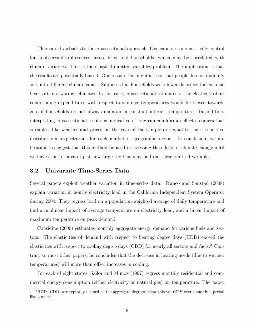
There are drawbacks to the cross-sectional approach. One cannot econometrically control
for unobservable differences across firms and households, which may be correlated with
climate variables. This is the classical omitted variables problem. The implication is that
the results are potentially biased. One reason this might arise is that people do not randomly
sort into different climate zones. Suppose that households with lower disutility for extreme
heat sort into warmer climates. In this case, cross-sectional estimates of the elasticity of air
conditioning expenditures with respect to summer temperatures would be biased towards
zero if households do not always maintain a constant interior temperature. In addition,
interpreting cross-sectional results as indicative of long run equilibrium effects requires that
variables, like weather and prices, in the year of the sample are equal to their respective
distributional expectations for each market or geographic region. In conclusion, we are
hesitant to suggest that this method be used in assessing the effects of climate change until
we have a better idea of just how large the bias may be from these omitted variables.
3.2 Univariate Time-Series Data
Several papers exploit weather variation in time-series data. Franco and Sanstad (2008)
explain variation in hourly electricity load in the California Independent System Operator
during 2004. They regress load on a population-weighted average of daily temperature and
find a nonlinear impact of average temperature on electricity load, and a linear impact of
maximum temperature on peak demand.
Considine (2000) estimates monthly aggregate energy demand for various fuels and sec-
tors. The elasticities of demand with respect to heating degree days (HDD) exceed the
elasticities with respect to cooling degree days (CDD) for nearly all sectors and fuels.3 Con-
trary to most other papers, he concludes that the decrease in heating needs (due to warmer
temperatures) will more than offset increases in cooling.
For each of eight states, Sailor and Munoz (1997) regress monthly residential and com-
mercial energy consumption (either electricity or natural gas) on temperature. The paper
3HDD (CDD) are typically defined as the aggregate degrees below (above) 65◦F over some time periodlike a month.
8
tests whether season-specific linear functions of temperature or functions of HDD and CDD
better fit the data. Lam (1998) also uses time-series data for Hong Kong and finds an elas-
ticity of annual electricity demand with respect to cooling degree days of 0.22, though prices
are assumed exogenous.
There are a few general concerns with using time series data. First, they only address the
short run response to changes in weather and cannot address long run adaptation. Second,
aggregate data cannot control for unobserved factors also changing over time. If the income
distribution or business composition change over time, data may be used as control variables.
However, unobservable factors cannot be taken into account. These omitted variables may
cause bias, just like in the case of the cross sectional analysis. In contrast to that literature,
time series data cannot only measure the intensive margin. We conclude that this literature
is the least likely to be informative on climate damages.
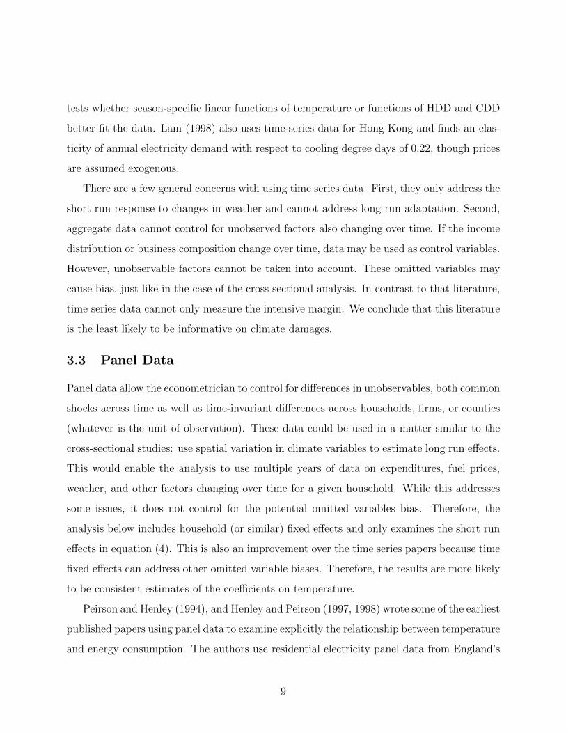
3.3 Panel Data
Panel data allow the econometrician to control for differences in unobservables, both common
shocks across time as well as time-invariant differences across households, firms, or counties
(whatever is the unit of observation). These data could be used in a matter similar to the
cross-sectional studies: use spatial variation in climate variables to estimate long run effects.
This would enable the analysis to use multiple years of data on expenditures, fuel prices,
weather, and other factors changing over time for a given household. While this addresses
some issues, it does not control for the potential omitted variables bias. Therefore, the
analysis below includes household (or similar) fixed effects and only examines the short run
effects in equation (4). This is also an improvement over the time series papers because time
fixed effects can address other omitted variable biases. Therefore, the results are more likely
to be consistent estimates of the coefficients on temperature.
Peirson and Henley (1994), and Henley and Peirson (1997, 1998) wrote some of the earliest
published papers using panel data to examine explicitly the relationship between temperature
and energy consumption. The authors use residential electricity panel data from England’s
9
Electricity Management Unit Demonstration Project pricing experiment from April 1989
to March 1990. Not only do extreme temperatures increase consumption, they also note
that price elasticities change with temperature: moving away from 50◦F results in less own-
and cross-price elastic demand. The reverse is also the case: higher prices reduce consumers’
temperature elasticities. Both effects are important for climate change and are not frequently
mentioned.
In addition to these micro data studies, there have been some studies using panel data
where demand is aggregated across consumers by Chinese province (Asadoorian et al., 2008)
or nation (Eskeland and Mideksa, 2010, and De Cian et al., 2007). Asadoorian et al. (2008)
model both the extensive margin (appliance choice for AC, fans, refrigerators, and TVs),
as well as the intensive margin (electricity consumption) in the short run.4 Eskeland and
Mideksa (2010) study European countries’ annual electricity demand. With aggregate data
they recognize that electricity prices and income are endogenous and use the per-kWh value
added tax rate and the total value added taxes in the economy as instruments. They find
extremely small effects of temperature on consumption.5 De Cian et al. (2007) use the
Arellano-Bond (1991) estimator to study European countries’ annual energy use. Studies
using aggregate data introduce a similar critique as the literature of the two previous sub-
sections: omitted variables may be correlated with changes over time within a province or
country. Without fixed effects at the level of the consumer, we cannot be confident that
these results are unbiased even with instrumental variables.
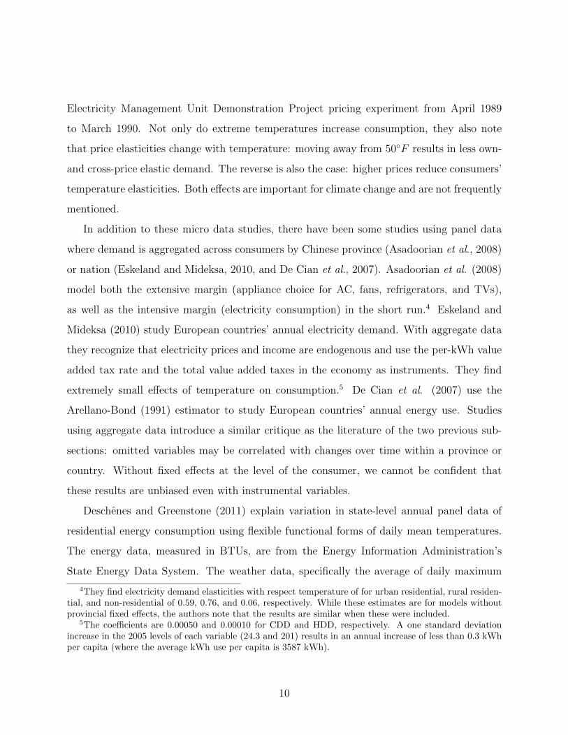
Deschenes and Greenstone (2011) explain variation in state-level annual panel data of
residential energy consumption using flexible functional forms of daily mean temperatures.
The energy data, measured in BTUs, are from the Energy Information Administration’s
State Energy Data System. The weather data, specifically the average of daily maximum
4They find electricity demand elasticities with respect temperature of for urban residential, rural residen-tial, and non-residential of 0.59, 0.76, and 0.06, respectively. While these estimates are for models withoutprovincial fixed effects, the authors note that the results are similar when these were included.
5The coefficients are 0.00050 and 0.00010 for CDD and HDD, respectively. A one standard deviationincrease in the 2005 levels of each variable (24.3 and 201) results in an annual increase of less than 0.3 kWhper capita (where the average kWh use per capita is 3587 kWh).
10
and minimum temperature, are from the National Climatic Data Center Summary of the
Day Data (File TD-3200). The identification strategy behind their paper relies on random
fluctuations in weather to identify climate effects on residential energy consumption (Cst).
The model includes state fixed effects (αs), census division by year fixed effects (γdt), and
flexible functions of precipitation, population and income, f(Xst; β). The mean daily tem-
perature data (TMEANstj) enter the model as the number of days in bin j for state s and
year t, where j is one of several pre-determined temperature intervals. For idiosyncratic
shock εst, they model log consumption as:
ln(Cst) =∑j
θTMEANj TMEANstj + f(Xst; β) + αs + γdt + εst. (8)
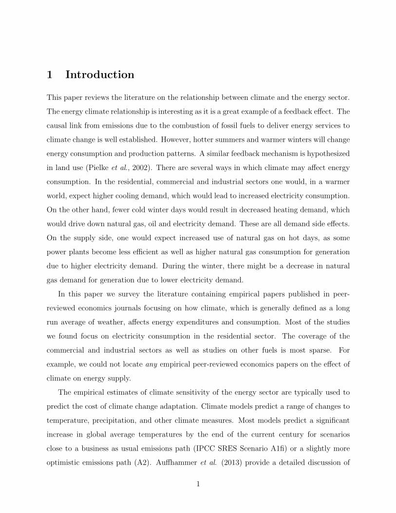
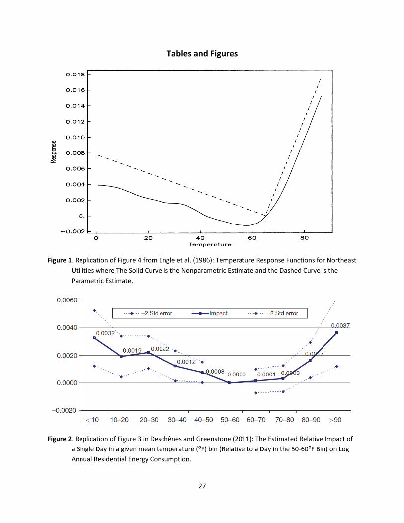
The authors find a U-shaped response function where electricity consumption is higher on
very cold and hot days (see Figure 2). They conclude that “business-as-usual” climatic
predictions for 2099 will increase residential energy consumption by 11 percent. Their are
two concerns with this study that were also mentioned for several other papers above. First,
responses to weather shocks only estimate the intensive margin. Second, aggregate data
mask changes in composition of households and industry that more detailed-level data could
address.
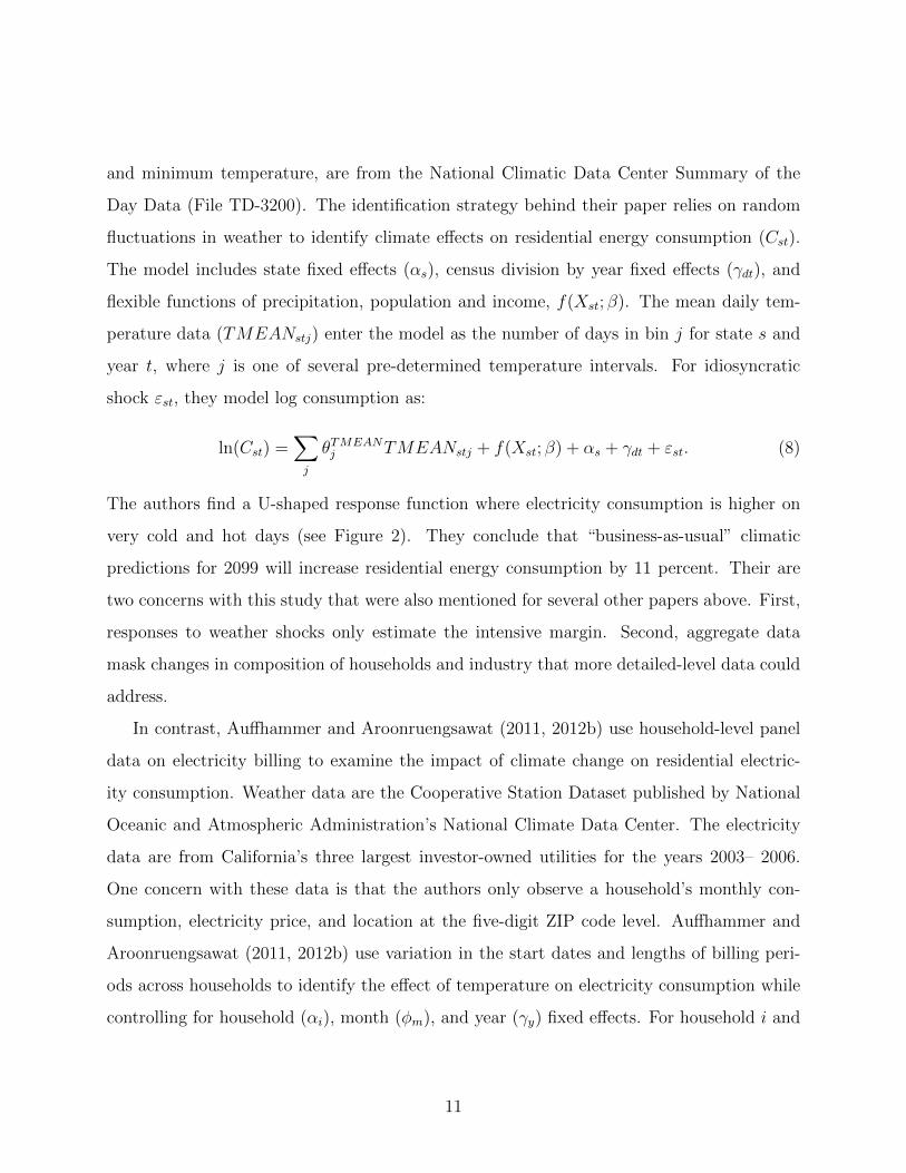
In contrast, Auffhammer and Aroonruengsawat (2011, 2012b) use household-level panel
data on electricity billing to examine the impact of climate change on residential electric-
ity consumption. Weather data are the Cooperative Station Dataset published by National
Oceanic and Atmospheric Administration’s National Climate Data Center. The electricity
data are from California’s three largest investor-owned utilities for the years 2003– 2006.
One concern with these data is that the authors only observe a household’s monthly con-
sumption, electricity price, and location at the five-digit ZIP code level. Auffhammer and
Aroonruengsawat (2011, 2012b) use variation in the start dates and lengths of billing peri-
ods across households to identify the effect of temperature on electricity consumption while
controlling for household (αi), month (φm), and year (γy) fixed effects. For household i and
11
billing period t, they estimate the following equation:
lnCit =∑j
θTMEANj TMEANitj + f(Xit; β) + αi + φm + γy + εit, (9)
where f(Xit; β) is a flexible function of precipitation and (in some specifications) household
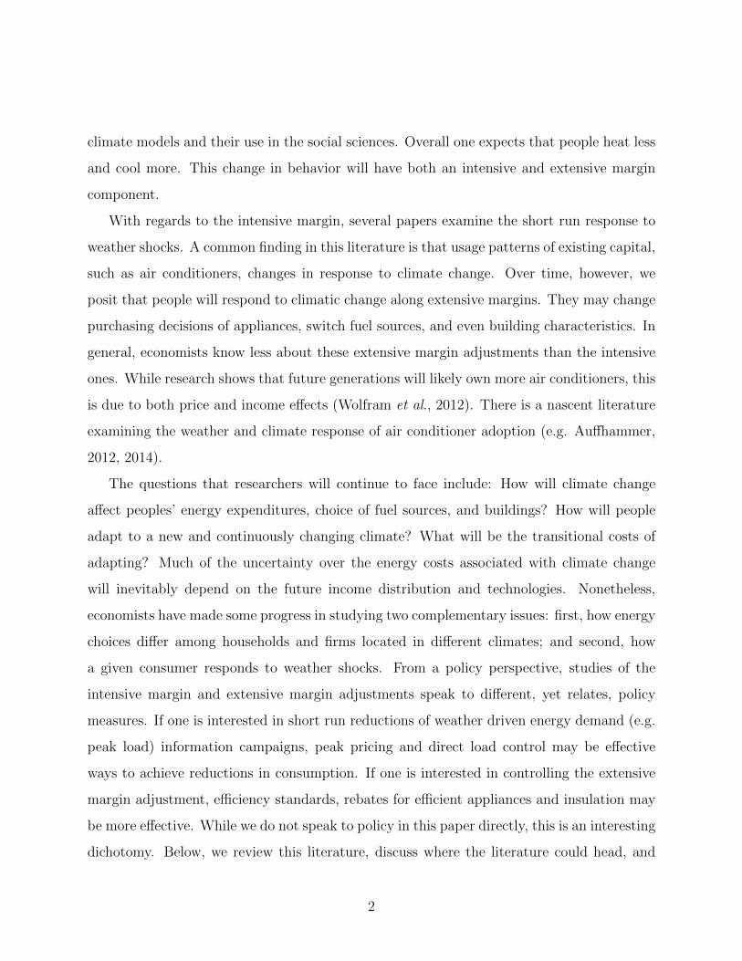
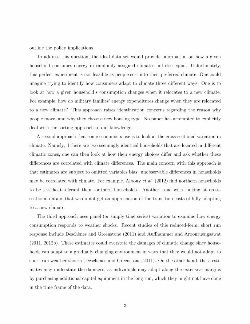
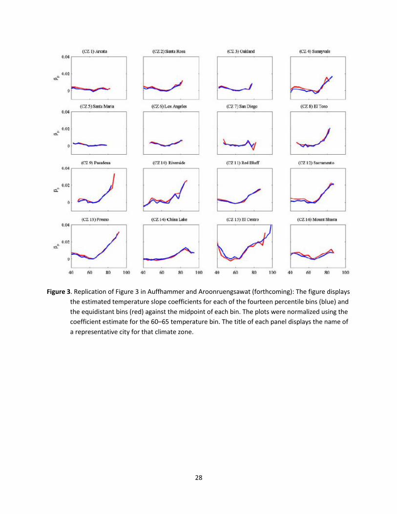
average monthly prices. Importantly, they estimate this model separately for each climate
zone (see Figure 3). Unfortunately, these data are only for California and may not be
representative of other US regions or other industrialized countries.
We conclude that using panel data is the most promising method for estimating the effect
of weather on energy expenditures. The first caveat raised with temperature still remains:
the papers only address the short run response to changes in weather and cannot address
long run adaptation. Nonetheless, the omitted variables issue that was raised for both the
cross section and time series data is less likely to be an issue in this work.
4 Moving the Literature Forward
We see this literature progressing on two related fronts. On the intensive margin, economists
can continue to refine the panel data estimates of how consumption and expenditures re-
spond to weather shocks. In particular, building on Auffhammer and Aroonruengsawat
(2011, 2012b), the literature could ask how these response functions differ by climate zone.
Detailed, high-frequency micro data on households’ and firms’ energy expenditures over large
geographic areas would provide substantial variation that would allow for the greatest un-
derstanding of how people respond to weather. Furthermore, understanding the likelihood
of relevant weather events in a given climate zone is important in thinking about how these
estimates apply to scenarios with climatic change. On the extensive margin, there is much to
be learned. In particular, economists can work to improve our understanding of how building
characteristics - like air conditioning, fuel choice, and insulation and other energy-efficiency
technologies - vary with climate. The only well-developed literature on the extensive margin
responses looks at the adoption of air conditioners. There is a significant opening for studies
looking at investments in other building characteristics. Due to this literature constraint,
12
we now turn to describing what has been written on air conditioning adoption as we see this
as a significant part of how research on climate adaptation and energy use can proceed.
4.1 Air Conditioner Adoption and the Extensive Margin
Most empirical papers on air conditioner adoption–largely due to data availability concerns–
estimate models based on cross sections or repeated cross sections. Data collection efforts
enabling panel data methods will add a meaningful dimension to this literature. The litera-
ture examining the adoption of air conditioners in response to changes in climate is essentially
non-existent. There is a much longer literature looking at empirical models of durable goods
adoption as a function of incomes, fixed and variable costs. Surveying these approaches
taken to better understand the impact of income and prices on adoption provides a useful
overview of the methods employed in this literature nonetheless. We review the literature
for the United States, Europe, and in developing countries.
4.2 Air Conditioning Adoption in the United States
In the early 1950s in the United States, air conditioners were mainly found in movie theaters,
supermarkets, and other public spaces (Biddle, 2008). Less than two percent of households
owned air conditioners in 1955. By 1980, the residential penetration rate rose to 50 percent,
with half of these households having installed central air conditioning units. There was
significant heterogeneity in the penetration, where half of the residences in the Northeast were
air-conditioned and some urban areas in Texas and Florida had penetration rates in excess
of 90 percent. What is relevant to the discussion in this paper is the relative importance
of weather/climate over changes in policy, population movements, income, prices or air
conditioners and electricity in the adoption decision.
There was much movement in all of these confounders since the 1950s. On the policy front
in 1957 “the Federal Housing Authority announced that the cost of air conditioning could be
rolled into approved mortgage packages, which led to a jump in installations.” Biddle (2008)
also addresses the concern raised above about the importance of sorting and population
13
movements. He provides an interesting back-of-the-envelope calculation suggesting that the
extensive population shifts during this period can only account for a fraction of the changes
in penetration over time. He also documents significant changes in prices, by showing that
after adjusting for efficiency gains and inflation, the price of air conditioners dropped by 25
percent during the 1970s and another 20 percent during the 1980s. While AC prices fell,
electricity prices were volatile: they dropped significantly during the 1950s and 1960s and
then rose again during the 1970s. During this entire period incomes rose substantially, which
suggests that the falling costs of installation and operation combined with rising incomes
drove the adoption of air conditioners during this period.
In order to determine the relative importance of these factors, Biddle (2008) matches
the air conditioning indicators with the corresponding socioeconomic characteristics from
three Census cross sections for 1960, 1970 and 1980 to electricity rates in the Standard
Metropolitan Statistical Area (SMSA), incomes and detailed climate variables (e.g. Cooling
and Heating Degree Days, wind speed, relative humidity). He uses a reduced form econo-
metric model, which accounts for changes in incomes, prices and weather in order to explain
the heterogeneity in penetration.
Biddle shows that differences in climate across SMSAs explain 75-95 percent as much of
the variation in penetration in the cross section relative to the models, which also control
for prices and socioeconomic factors. He also shows that the home characteristics relevant
to retrofitting played a significant role.
Sailor and Pavlova (2003) use data on air conditioning penetration for 39 US cities to
parameterize a relationship between cooling degree days and market saturation. They take
issue with existing estimates that electricity consumption rises by two to four percent for each
degree Celsius in warming as these estimates only account for intensive margin adjustments
(more frequent operation of existing air conditioning equipment). A hotter future will result
in extensive margin adjustments, namely higher saturation levels. They use penetration
data from the American housing survey for 39 cities for the year 1994-1996 for both central
and window units. They show that a significant number of cities have air conditioning
14
penetration below 80 percent suggesting that there is room for two temperature driven
margins of adjustment under climate change: Increased adoption of air conditioners and
increased usage. Ignoring the adoption decision would lead to an underestimation of future
electricity consumption. They estimate a relationship between saturation and cooling degree
days for the combined saturation plot. They estimate an equation between what they call
saturation (which is the recent penetration from the 1994-1996 American Housing Survey)
and cooling degree days of the form:
So = 0.944− 1.17 exp(−0.00298 · CDD) (10)
This simple relationship does not control for any other observables (such as income) or
other climate factors. Further, no standard errors are provided so it is not clear whether the
relationship is statistically significant. To model consumption, the authors explain variation
in state per capita electricity consumption as a proxy for city level per capita consumption
using CDDs, HDDs and wind speed. It is shown that higher CDDs lead to increased adop-
tion of air conditioners and higher use. Adding the extensive margin adjustment results in
increases that are significant and matter when making forecasts. Sailor and Pavlova (2003)
note that “Based on these results, Los Angeles’ per capita residential electricity consumption
is projected to increase by eight percent in July for a 20 percent increase in CDD. If the
market saturation were assumed to remain constant, however, the projection would be for
only a five percent increase.”
Rapson (2011) estimates a state of the art discrete-time, infinite horizon dynamic con-
sumer optimization problem. In his structural model, consumers in each period decide
between buying a maximum of one unit of a durable good and the amount of household
production. An interesting and important feature of his model is that households operate in
an environment of uncertainty, where they do not know the efficiency of a durable bought
in a future period and may therefore wait to purchase until technological progress has hap-
pened. In a “first stage”, he estimates derived demand for electricity from central and room
air conditioners. He uses five cross sections of the Energy Information Administration’s Res-
15
idential Electricity Consumer Survey (RECS), which he matches to air conditioner prices
and efficiencies. His first stage derived demand elasticities are consistent with more general
estimated of electricity demand. For central air conditioners the estimates price elasticity of
derived demand is -0.170 for the whole sample and drops to -0.068 if one drops California.
The income elasticities for both samples are 0.21. The cooling degree elasticities are near
unity (0.989 for the whole sample and 0.961 once he drops California from the sample). For
room air conditioners, the price elasticity for both samples is higher (-0.34 for both samples)
The cooling degree elasticities are also higher at 1.07 for all states and 1.092 for the sample
dropping California. The income elasticities are 0.114 and 0.126 respectively. These estima-
tion results for derived electricity demand are precisely estimated and consistent with the
prior literature.
Rapson (2011) then goes on to estimate unit demand elasticities with respect to electric-
ity price, unit efficiency and purchase price of the units. His estimates suggest significant
responsiveness in the adoption of room and central air conditioners with respect to efficiency.
The elasticities for central AC range from 0.7 to 1 and for room AC range from 0.2 to 0.3.
The estimated elasticities with respect to purchase price are lower. For central air condi-
tioning they are clustered around -0.241 and for room units they range from -0.12 to -0.13.
The elasticities with respect to electricity prices are small for and not statistically significant
for central unit adoption (-0.024) and bigger and significant for room unit adoption (-0.220;
-0.35). This is an innovative structural paper, which exploits the time dimension of the
repeated cross sections and arrives at credible and precisely estimated coefficients for both
intensive and extensive margin adjustments.
While the data for the 2011 RECS survey have not been fully released at the writing of
this paper, the Energy Information Administration (EIA, 2011) shows a preview of the data
which displays further growth in air conditioner penetration on the US. Time series show
little slowdown in the growth of air conditioner penetration. 87 percent of US households had
air conditioning in 2009, which is the latest year of data. The EIA (2011) notes that “wider
use has coincided with much improved energy efficiency standards for AC equipment, a
16
population shift to hotter and more humid regions, and a housing boom during which average
housing sizes increased.” However, the continued growth of air conditioner penetration puts
in question using a cross section of current penetration levels as “saturation” proxies for other
regions with similar climate characteristics based on the equation by Sailor and Perova (2003)
above. As we will see in the next sections, cross sectional US data are used to parameterize
relationships which determine climate dependent saturation levels in other countries.
EIA (2011) also shows that there is little variation in usage over the summer. This
is when the percentage of households using AC during the summer is between 30 and 40
percent, except in the South, where 67 percent of households run their air conditioners all
summer. Further, newer homes are most likely to have central AC, whereas older homes are
more likely to have no air conditioning or window units as retrofitting with central AC has
non-trivial transactions costs. EIA (2011) further notes that there is significant heterogeneity
in the penetration and type of AC units installed across the income spectrum, which is not
surprising given the high cost of installing central air.
4.3 Air Conditioning Adoption in Europe
In Europe, data on air conditioner usage and adoption are scarce and the literature we
could gain access to is thin as a result. Much of the literature on changing energy demand in
Europe as a consequence of climate change focuses on decreasing demand for heating instead
of the increased demand for cooling. What is even more surprising was the apparent lack of
publicly available data and studies at member country level. Given the predicted shifts in
climate for EU member countries and the relatively high incomes, a better understanding
of intra-European adoption patterns is very important to better project future electricity
demand in the European Union.
The maybe most informative report is a study by the Directorate-General for Mobility
and Transport (European Commission) published in 2003, which provides an overview of
the penetration of central air conditioners (CACs) and their efficiencies across EU member
states. Central air conditioners here are defined as air conditioning systems with more than
17
12 kW of cooling capacity, which does not include smaller room type air conditioners. The
report indicates that the area cooled per inhabitant is expected to rise rapidly from 3m2 per
inhabitant in 2000 to 5m2 per inhabitant by 2010. Recent data indicate almost a quintupling
in CAC area in the EU over the past 20 year period. The rapid growth is driven by expansion
of cooled floor area in Italy and Spain, which now are responsible for more than 50 percent of
the cooled floor area. If one normalizes cooled area by population, the distribution of cooled
square meters per person is highly correlated with summer temperatures. This report only
discusses the cross sectional variation, when in fact how these measures have developed over
time would enable us to better understand the drivers of these series–especially the relative
roles of rising incomes versus changing temperatures.
Aebischer et al. (2007) provide another study predicting energy demand for Europe under
climate change. The paper is not very clear on how predictions are calculated and focuses
much on the trade-off between heating and cooling demand thereafter. Given the climate
heterogeneity in Europe and predicted warming throughout the continent combined with the
member countries relatively high incomes, further studies of changing air conditioner pene-
tration and collection of data could provide important insights into the future of European
energy demand.
A concerted effort, if not already underway, to collect and analyze data for Europe
similar to what Rapson (2011) or Biddle (2008) did for the US would be insightful, given
the tremendous degree of heterogeneity in weather, electricity prices and incomes across the
European Union member states. While the penetration of air conditioners in central and
northern Europe is very small, under climate change these rates can potentially grow rapidly
with significant impacts on electricity consumption and the load profile. Given a shift away
from nuclear power for base load in e.g. Germany, these shifts could have significant impacts
on load profiles and the ability of generators to meet peak demand.
18

4.4 Air Conditioning Adoption in Developing Countries
McNeil and Letschert (2010) provide a model of adoption of air conditioners and appliances
using cross-country data. They incorporate the fact that saturation levels are climate depen-
dent, which is the idea raised in Sailor and Pavlova (2003). They have collected appliance
penetration levels across countries from a number of micro level surveys–most of which are in
the LSMS database of the WorldBank for various years (mostly late 1990s and early 2000s).
McNeil and Letschert (2008) discuss these data in more detail. In a first step, they estimate
a relationship between saturation (which they call “Climate Maximum”) and cooling degree
days for 39 US cities. They then use this estimated relationship to estimate a predicted
saturation level based on cooling degree days for a given location. For developing country
locations in their sample air conditioner saturation is assumed to approach this frontier,
but never exceed it. They then model diffusion of air conditioners as a function of income,
conditional on a location’s Climate Maximum, which is a function of CDD. The diffusion
equation for air conditioners is given by:
log
(Climate Maximumi
Diffi− 1
)= log γ + βincInci (11)
What is different in this equation is that Climate Maximum is the cooling degree de-
pendent saturation level based on the cross section of US cities discussed above. For other
appliances, such as refrigerators, a common value (e.g. 1 per household) is used. If the cli-
mate maximum for a given country is one and the saturation is one, penetration is therefore
100 percent. If the climate maximum is 0.1 and the saturation is 0.1, penetration is also 100
percent. Their regression is based on 24 observations.
They explain 70 percent of the variation in the transformed dependent variable, which
means that their model fits the cross sectional data fairly well. What is noteworthy about
the estimated adoption curve is that the penetration rates are very low and clustered around
zero for a number of countries. At income levels of $25,000 the adoption rates seem to rise
drastically. While the modeling approach here is appealing and the data collection effort is
impressive, this is essentially a cross sectional regression which cannot meaningfully control
19
for confounding factors. Using repeated cross sections or panel data on this model would
allow one to separate out unobservables via a two-way fixed or random effects strategy.
Isaac and van Vuuren (2009) build on the model by McNeil and Letschert (2010) but
in addition endogenize the unit energy consumption (UEC) as a function of income, which
allows for income dependent energy efficiency of air conditioners. They then predict pene-
tration rates based on CDD and income, which allows them to build regional predictions.
They show that their model can predict US penetration very well, but is off by 30 percent
for Japan.
Akpinar-Ferrand and Singh (2010) look at air conditioning demand for India. The authors
used a combination of AC ownership data from the NSS 55 survey (2001) and obtained sales
data from industry sources. They follow the same approach as Isaac and van Vuuren (2009)
described above. The combination of rapidly rising incomes and a hot and in many cases
humid climate has led to very fast growth in sales in urban areas with a relatively reliable
electricity supply. Rural area adoption has lagged as only 44 percent of rural households
have access to electricity. The authors predict a rapid rise in the penetration rates of air
conditioners over the next century.
What would be of great interest are studies, which project future air conditioner penetra-
tion by country by 2100 under different climate, income and price scenarios. Unfortunately
our understanding of air conditioner penetration by country is very limited, which makes
issuing these projections a challenging yet important task.
5 Conclusion
This paper reviews the literature on the relationship between climate and the energy sector.
In particular, we primarily discuss empirical papers published in peer-reviewed economics
journals focusing on how climate affects energy expenditures. Climate will affect energy
consumption by changing how consumers respond to short run weather shocks (the intensive
margin) as well has how people will adapt in the long run by changing durable goods (the
extensive margins).
20
Along the intensive margin, we conclude that much of the existing literature has been
limited to time series variation or aggregated panel data. Both raise concerns of omitted
variables bias. Until recently, few studies used household-level panel data and even those
are informative of only a small part of the world. Further research that uses household-
level panel data of energy consumption may help identify how consumers around the world
respond to weather shocks. Research on technology adoption, like air conditioning use, will
further our understanding of the extensive margin.
The current literature has made some progress in these dimensions. The coefficient
estimates from papers like Deschenes and Greenstone (2011) and Auffhammer and Aroon-
ruengsawat (2011, 2012b) offer some of the best evidence we have on the intensive margin.
We have not identified any paper that identify the extensive margin using panel data. As
such, the implications for policy makers are muted. What we would like to be able to identify
for policy makers and integrated assessment modelers is a reduced-form, long run response
coefficient. It is not clear to us how this can be credibly estimated.
Finally, we recognize that there is great uncertainty about the future. If we are to learn
about the extensive margin, it is important to keep in mind that these capital investments are
being made in the context of a continuously changing and uncertain climate. One factor that
we are uncertain over is technology. We do know, however, that changing the climate will
induce technological change. Some technologies that are not economic today may become
so in the future. For example, at some price even hydrogen fuel cells, which could end the
positive feedback loop between climate and energy use, would become viable. These futures
possibilities are not measured in the empirical literature we discussed in this paper, but are
important to consider in a broader context.
21

Appendix on Related Literatures
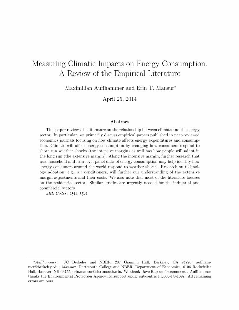
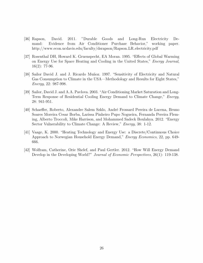
Economists have written extensively on the estimation of electricity demand. In estimatingprice elasticity, many papers recognize the importance of controlling for weather shocks (e.g.,Lee and Chiu 2011). Some early studies even focused explicitly on the relationship betweenweather and electricity sales: Engle et al. (1986) estimate electricity demand response totemperature for four US utilities. Rather than imposing linearity in HDD and CDD, theauthors allow for flexible temperature responses using cubic and piecewise linear splines (seeFigure 1). In contrast to current papers focusing on climate change, their motivation forunderstanding this relationship was because weather-adjusted sales are used in regulatoryrate hearings. For this reason we do not include them in the body of the paper. Nonetheless,the findings from these types of studies could be used in evaluating the impacts climate onenergy demand.
An alternative to the econometric methods discussed in Section 3 would be to use en-gineering methods to map temperature into expenditures. For example, Rosenthal andGruenspecht (1995) take climate model predictions of changes in heating and cooling degreedays and calculate the resulting changes in US energy expenditures. In contrast to the ma-jority of studies mentioned, they predict a reduction in expenditures due to a temperatureincrease. This approach, however, is based on technology, not on human behavior.
22
References
[1] Aebischer, Bernard, Giacomo Catenazzi, and Martin Jakob. 2007. “Impactof Climate Change on Thermal Comfort, Heating and Cooling Energy De-mand in Europe,” Proceedings ECEEE 2007 Summer Study “Saving En-ergy – Just do it!” La Colle sur Loup, France. ISBN: 978-91-633-0899-4.http://www.cepe.ethz.ch/publications/Aebischer 5 110.pdf
[2] Akpinar, Ferrand, E., and A. Singh. 2010. “Modeling Increased Demand of Energyfor Air Conditioners and Consequent CO2 Emissions to Minimize Health Risks Due toClimate Change in India,” Journal of Environmental Science and Policy, 13(8): 702-712.
[3] Albouy, D., Graf, W. F., Kellogg, R., & Wolff, H. (2013). Climate amenities, climatechange, and American quality of life (No. w18925). National Bureau of Economic Re-search.
[4] Arellano, M. and S. Bond. 1991. “Some Tests of Specification for Panel Data: MonteCarlo Evidence and an Application to Employment Equations,” The Review of Eco-nomic Studies, 58(2): 227-297.
[5] Asadoorian, Malcolm O., Richard S. Eckaus, C. Adam Schlosser. 2008. “Modeling Cli-mate feedbacks to Energy Demand: The Case of China,” Energy Economics, 30(4):1577-1602.
[6] Auffhammer, Maximilian. 2012. “Hotspots of climate driven increases in residentialelectricity demand: A simulation exercise based on household level billing data forCalifornia,” California Energy Commission White Paper CEC5002012021.
[7] . 2014. “Cooling China: The Weather Dependence of Air Conditioner Adop-tion,” Frontiers of Economics in China.
[8] Auffhammer, Maximilian and Anin Aroonruengsawat. 2011. “Simulating the Impactsof Climate Change, Prices and Population on California’s Residential Electricity Con-sumption,” Climatic Change, 109(S1): 191-210.
[9] . 2012b. “Erratum to: Simulating the Impacts of Climate Change, Pricesand Population on California’s Residential Electricity Consumption,” Climatic Change,113(3-4), pp 1101-1104.
[10] Auffhammer, Maximilian, Solomon M. Hsiang, Wolfram Schlenker, and Adam Sobel.2013. “Using weather data and climate model output in economic analyses of climatechange,” Review of Environmental Economics and Policy, 7(2), 181-198.
[11] Biddle, Jeff. 2008. “Explaining the Spread of Residential Air Conditioning, 1955-1980,”Explorations in Economic History, 45: 402-423.
23
[12] Considine, Timothy. 2000. “The Impacts of Weather Variations on Energy Demand andCarbon Emissions,” Resource and Energy Economics, 22: 295–314.
[13] De Cian, Enrica, Elisa Lanzi, and Roberto Roson. 2007. “The Impact of TemperatureChange on Energy Demand: A Dynamic Panel Analysis,” Fondazione Enrico MatteiWP 2007-46. http://www.feem.it/userfiles/attach/Publication/NDL2007/NDL2007-046.pdf
[14] Deschenes, Olivier and Michael Greenstone. 2011. “Climate Change, Mortality, andAdaptation: Evidence from Annual Fluctuations in Weather in the US,” AmericanEconomic Journal: Applied Economics, 3(4): 152–185.
[15] Directorate General Transportation Energy of the Commission of the European Union.2003. Energy Efficiency and Certification of Central Air Conditioners. Final ReportApril 2003. Volume 1.
[16] Dubin, Jeffrey A. and Daniel L. McFadden. 1984. “An Econometric Analysis of Resi-dential Electric Appliance Holdings and Consumption,” Econometrica. 52(2): 345-362.
[17] Energy Information Administration. 2011. “Air Con-ditioning in Nearly 100 Million U.S. Homes,” seehttp://www.eia.gov/consumption/residential/reports/air conditioning09.cfm
[18] Engle, Robert F., C. W. J. Granger, John Rice, and Andrew Weiss. 1986. “Semipara-metric Estimates of the Relation between Weather and Electricity Sales,” Journal ofthe American Statistical Association, 81(394): 310–320.
[19] Eskeland, Gunnar S. and Torben K. Mideksa. 2010. “Electricity Demand in a ChangingClimate,” Mitig Adapt Strateg Glob Change. 15: 877–897.
[20] Franco, Guido and Alan Sanstad. 2008. “Climate Change and Electricity Demand inCalifornia,” Climatic Change, 87(Suppl 1): S139–S151.
[21] Henley, Andrew and John Peirson. 1997. “Non-Linearities in Electricity Demand andTemperature: Parametric vs. Non-parametric Methods,” Oxford Bulletin of Economicsand Statistics, 59(1): 149-162.
[22] . 1998. Residential Energy Demand and the Interaction of Price Temperature:British Experimental Evidence, Energy Economics, 20: 157-171.
[23] Isaac, Morna and Detlef P. Van Vuuren. 2009. “Modeling Global Residential SectorEnergy Use for Heating and Air Conditioning in the Context of Climate Change,”Energy Policy, 37: 507-521.
[24] Lam, Joseph C. 1998. “Climatic and Economic Influences on Residential ElectricityConsumption,” Energy Conversion and Management, 39(7): 623-629.
24
[25] Lee, Chien-Chiang and Yi-Bin Chiu. 2011. “Electricity Demand Elasticities and Temper-ature: Evidence from Panel Smooth Transition Regression with Instrumental VariableApproach,” Energy Economics, 33(5): 896-902.
[26] Mansur, Erin T., Robert Mendelsohn, and Wendy Morrison. 2008. “Climate ChangeAdaptation: A Study of Fuel choice and Consumption in the US Energy Sector,” Journalof Environmental Economics and Management, 55(2): 175–193.
[27] McNeil, Michael A. and Virginie E. Letschert. 2010. “Model-ing Diffusion of Electrical Appliances in the Residential Sector,”http://www.osti.gov/bridge/servlets/purl/985912-HSB5Kt/985912.pdf
[28] . 2008. “Future Air Conditioning Energy Consumption in Developing Coun-tries and what can be done about it: The Potential of Efficiency in the ResidentialSector,” ECEEE Summer Study, Cote d’Azur, France.
[29] Mendelsohn, Robert. 2001. “Energy: Cross-Sectional Analysis,” Global Warming andthe American Economy: A Regional Analysis. Robert Mendelsohn (ed.) Edward ElgarPublishing, England.
[30] Mendelsohn, Robert. 2006. “Energy Impacts,” The Impact of Climate Change on Re-gional Systems: A Comprehensive Analysis of California. Joel Smith and RobertMendelsohn (eds.) Edward Elgar Publishing, Northampton, MA.
[31] Mideksa, Torben and Steffen Kallbekken. 2010. “The Impact of Climate Change on theElectricity Market: A Review,” Energy Policy, 38: 3579-3585.
[32] Morrison, Wendy and Robert Mendelsohn. 1999. “The Impact of Global Warming onUS Energy Expenditures,” The Impact of Climate Change on the United States Econ-omy. Robert Mendelsohn and James Neumann (eds.) Cambridge University Press, Cam-bridge, UK.
[33] Nakicenovic, Nebojsa, and Robert Swart. ”Special report on emissions scenarios.” Spe-cial Report on Emissions Scenarios, Edited by Nebojsa Nakicenovic and Robert Swart,pp. 612. ISBN 0521804930. Cambridge, UK: Cambridge University Press, July 2000. 1(2000).
[34] Peirson, John and Andrew Henley. 1994. “Electricity Load and Temperature: Issues inDynamic Specification,” Energy Economics, 16: 235-243.
[35] Pielke, R. A., Marland, G., Betts, R. A., Chase, T. N., Eastman, J. L., Niles, J. O., &Running, S. W. (2002). The influence of land-use change and landscape dynamics onthe climate system: relevance to climate-change policy beyond the radiative effect ofgreenhouse gases. Philosophical Transactions of the Royal Society of London. Series A:Mathematical, Physical and Engineering Sciences, 360(1797), 1705-1719.
25
[36] Rapson, David. 2011. ”Durable Goods and Long-Run Electricity De-mand: Evidence from Air Conditioner Purchase Behavior,” working paper.http://www.econ.ucdavis.edu/faculty/dsrapson/Rapson LR electricity.pdf
[37] Rosenthal DH, Howard K. Gruenspecht, EA Moran. 1995. “Effects of Global Warmingon Energy Use for Space Heating and Cooling in the United States,” Energy Journal,16(2): 77-96.
[38] Sailor David J. and J. Ricardo Munoz. 1997. “Sensitivity of Electricity and NaturalGas Consumption to Climate in the USA—Methodology and Results for Eight States,”Energy, 22: 987-998.
[39] Sailor, David J. and A.A. Pavlova. 2003. “Air Conditioning Market Saturation and Long-Term Response of Residential Cooling Energy Demand to Climate Change,” Energy,28: 941-951.
[40] Schaeffer, Roberto, Alexandre Salem Szklo, Andre Frossard Pereira de Lucena, BrunoSoares Moreira Cesar Borba, Larissa Pinheiro Pupo Nogueira, Fernanda Pereira Flem-ing, Alberto Troccoli, Mike Harrison, and Mohammed Sadeck Boulahya. 2012. “EnergySector Vulnerability to Climate Change: A Review,” Energy, 38: 1-12.
[41] Vaage, K. 2000. “Heating Technology and Energy Use: a Discrete/Continuous ChoiceApproach to Norwegian Household Energy Demand,” Energy Economics, 22, pp. 649-666.
[42] Wolfram, Catherine, Orie Shelef, and Paul Gertler. 2012. “How Will Energy DemandDevelop in the Developing World?” Journal of Economic Perspectives, 26(1): 119-138.
26
27
Tables and Figures
Figure 1. Replication of Figure 4 from Engle et al. (1986): Temperature Response Functions for Northeast Utilities where The Solid Curve is the Nonparametric Estimate and the Dashed Curve is the Parametric Estimate.
Figure 2. Replication of Figure 3 in Deschênes and Greenstone (2011): The Estimated Relative Impact of a Single Day in a given mean temperature (⁰F) bin (Relative to a Day in the 50-60⁰F Bin) on Log Annual Residential Energy Consumption.
28
Figure 3. Replication of Figure 3 in Auffhammer and Aroonruengsawat (forthcoming): The figure displays the estimated temperature slope coefficients for each of the fourteen percentile bins (blue) and the equidistant bins (red) against the midpoint of each bin. The plots were normalized using the coefficient estimate for the 60–65 temperature bin. The title of each panel displays the name of a representative city for that climate zone.