measures, trends and determinants of economic … · measures, trends and determinants of economic...
TRANSCRIPT
IARIW-Bank of Korea Conference “Beyond GDP: Experiences and Challenges in the
Measurement of Economic Well-being,” Seoul, Korea, April 26-28, 2017
MEASURES, TRENDS AND DETERMINANTS OF
ECONOMIC WELL-BEING IN INDIA
Protap Mukherjee (Young Lives India)
Paper prepared for the IARIW-Bank of Korea Conference
Seoul, Korea, April 26-28, 2017
Session 3B: Well-being in Asia
Time: Wednesday, April 26, 2017 [Afternoon]
1
Draft copy: please do not quote
MEASURES, TRENDS AND DETERMINANTS OF ECONOMIC WELL-BEING
IN INDIA
BY PROTAP MUKHRJEE*
This paper argues for three measures of economic well-being that includes other economic, health and
subjective dimensions besides households’ conventional wealth index and by using both pooled OLS
and random-effects regression estimates, this paper examines the levels of three measures of economic
well-being by time-invariant non-economic demographic, social and regional predictors. These
composite measures of economic well-being have shown that there are needs of serious policy
formulation must be aiming at particular groups who are being deprived of education, leisure, better
health and better subjective well-being over the years.
JEL Classification: I30, I32, P36, C33,
Keywords: well-being, economic, determinants, India, random-effects
1. Introduction
As GDP has major limitations which restrict its use as a measure of well-being, economists
and social scientists in recent times have become more interested in other measures of
economic well-being. GDP says nothing about the distribution of income between groups at a
point in time or about the distribution of income over time and it would be misleading to assess
the progress of a country or group of countries by looking by looking at only GDP (Atkinson
1969). Interestingly, economists and statisticians have always acknowledged the fact that it is
not a very good determinant of society’s wellbeing (Allin 2014).
Instead of attempting to evaluate economic well-being on the basis of only objective
indicators, subjective variables are often been considered in creating index of economic well-
being. This is especially helpful when one aims to study well-being by different background
variables like gender where utility based models of well-being are hard to apply. But if well-
being is judged by functionings, the contrast between position of men and women, can be
drawn and empirically studied (Sen 1999).
The widely used and but rather narrow measure of well-being is the United Nations
Development Programme (UNDP)’s annual Human Development Index (HDI) computed on
the basis of the levels of life expectancy, education and GDP and available for most of the
countries in the world. Of course the creation of such composite index from fundamentally
different indicators is a “bit like apple and oranges”, but its advantage lies in its simplicity and
its political power (Ray 2012). He further argued that there is a need to include indicators of
differential educational attainment, anthropometric indicators for nourishment, or indicators of
mortality or morbidity.
___________________ * Correspondence to: Protap Mukherjee, Research Coordinator, Young lives India, 47 Community
Centre, New Friends Colony, New Delhi: 110 065, India ([email protected])
2
Recent arguments on the topic are in support to use also subjective measures to enhance
the concept of economic well-being. Some of the subjective indicators discussed in literature
are happiness and its components, reduced unemployment rate, active civil society
participation and better health, among others.
Stiglitz, Sen and Fitoussi (2009) argues for a multidimensional definition of wellbeing
and states that among many, material living standards (as measured by income, consumption
and wealth), health status, education; and personal activities including work should be
considered simultaneously while examining well-being. As a result, this multi-dimensional
approach can give us a broader, more comprehensive understanding of the complex subject of
human living conditions (Cohen 2000, White 2010).
In fact, considering that well-being is multi-dimensional in nature, there is a scope to
include both objective and a subjective dimensions (Hallerod and Selden 2013, Schimmack et
al 2008). As a different approach for defining well-being, Hawkins (2014) argued that there is
a scope to utilize people’s feelings of wellbeing or satisfaction with their life directly in the
measurement. Subjective dimension like individual’s cognitive perception is equally relevant
because such a perception is able to reveal the subjective evaluation of quality of life (Haq and
Zia 2013) and clearly, the level of wellbeing of an individual or of a group may vary from one
area of life to another - and within areas of life (Levy and Guttman 1975). Obviously estimation
of the well-being remains a difficult task because of its multifaceted dimensions (Murias et. al.
2006).
. From the above perspectives, this paper aims to study economic well-being by
examining the following objectives:
1) To examine economic well-being by constructing three different measures or indices
and thereby to study these measures by different demographic, social and regional
background and also overtime.
2) To explore the non-economic determinants of the three measures of economic well-
being and thereby to compare the roles of the determinants across measures.
2. Data and Methods
2.1. Data
I use data from the Young Lives longitudinal survey in India which is a part of an international
study of childhood poverty following the lives of 12,000 children in Ethiopia, India (in the
states of Andhra Pradesh and Telangana), Peru and Vietnam over 15 years and coordinated out
of the Department of the International Development at the University of Oxford. The panel
survey follows two cohorts1 of children in each country. The first round was conducted in 2002,
followed by Round 2 in 2006, Round 3 in 2009 and Round 4 in 2013.
For this paper, I am using data relating to the Older Cohort households and children,
which consists of approximately 1,008 children who were first surveyed when they were
around the age of eight in Round 1. In Round 2 children were around 12 years old, in Round 3
the children were approximately 15 years old and in Round 4 children were around 19 years
old. For the present study, data from three rounds of quantitative Young Lives survey have
1 All Older Cohort children were born in 1994-95 and so at the time of Round 1 survey (2002) they were approximately 8 years old. On the other hand, Younger Cohort children who are not included in this paper were born in 2002-01 and were approximately 1 year old during Round 1 survey.
3
been utilized. The data collected in each round include both children and household
information on various topics; like assets in the households, education history, health status,
subjective wellbeing, time-use, occupation status, shocks etc. From all three rounds a total
sample of 2,853 households2 are examined.
For studying measure of economic well-being at household level, I focus on data related
to households’ assets, children’s time-use information on paid and unpaid work3, education,
health as measured by Body Mass Index (BMI)4 and subjective well-being5. The composite
measures of economic well-being are examined by seven socio-demographic and regional
characteristics variables or time-invariant predictors. They are gender of the household head,
place of residence, caste6 of the household head, religion of the household head, educational
level of the household head, base level household size7 and region8. The summary statistics for
these predictors are given in the Appendix (see Table A1).
2.2. Analytical strategy
2.2.1. Measures of economic well-being
First I use three different measures to study the magnitude of economic well-being at the
household level.
(1) The first measure I consider is wealth index which is a composite index that reflects
the welfare of household members in terms of the quality of the dwelling (for example, the
materials of the walls, roof etc.), use of durable goods (whether the household owns a radio,
TV, bicycle etc.), and access to basic services (whether the household has drinking water,
electricity, etc.). This index is already available in each round, so I use it as original as given
in the datasets and denoted by ew1.
(2) Then I build the second measure which is a composite index of previously used
wealth index (ew1) and newly added educational enrolment, labour force participation status
(separately for paid and unpaid work) and denoted by ew2.
(3) The third measure of economic well-being is constructed by adding two more
variable to ew2. These two variables cover health status (BMI) and subjective well-being scores
and denoted by ew3.
2 In Round 4 (2013), 951 households or children are surveyed and the responses are recorded. For a balanced panel, I consider only those households or children that were present in all three rounds and thus gives a panel of 2,853 (951*3) households or children. 3 Hours spent in domestic chores in a typical day is considered as the unpaid work. In Indian scenario, members of the households, especially women are usually engaged in unpaid domestic chores. In a pro-poor setting, this engagement is a proxy for poor economic prosperity as this limits children and adolescents’ opportunities for better educational and occupational achievements later. 4 Body Mass Index (BMI) is defined as ‘the weight in kilograms divided by the square of the height in metres (kg/m2)’ that is commonly used to classify underweight, overweight and obesity in adults (WHO 2016). Children whose BMI range from 18.50 to 24.99 are considered to have normal BMI. 5 Subjective well-being is calculated from the ‘ladder’ question that is asked in each round. This ladder is a scale that ranges from 1 to 9 where 1 represents the worst possible life and 9 is the best possible life. 6 There are four official caste groups in India as recognised by Constitution of India: Scheduled Caste (SC), Scheduled Tribes (ST), Backward Class (BC) and Other Castes (OC). 7 Household size in the Round 2 (2006) are considered as the base-level household size and treated as one time invariant variable. 8 Young Lives survey identified three regions in Undivided Andhra Pradesh: Coastal Andhra, Rayalaseema and Telangana. In July, 2014, Undivided Andhra Pradesh has been divided into two states: Andhra Pradesh and Telangana.
4
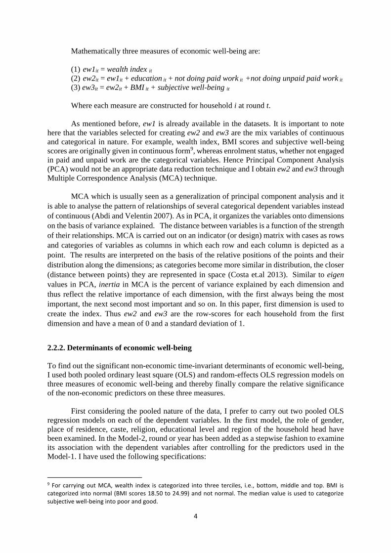
Mathematically three measures of economic well-being are:
(1) ew1it = wealth index it
(2) ew2it = ew1it + education it + not doing paid work it +not doing unpaid paid work it
(3) ew3it = ew2it + BMI it + subjective well-being it
Where each measure are constructed for household i at round t.
As mentioned before, ew1 is already available in the datasets. It is important to note
here that the variables selected for creating ew2 and ew3 are the mix variables of continuous
and categorical in nature. For example, wealth index, BMI scores and subjective well-being
scores are originally given in continuous form9, whereas enrolment status, whether not engaged
in paid and unpaid work are the categorical variables. Hence Principal Component Analysis
(PCA) would not be an appropriate data reduction technique and I obtain ew2 and ew3 through
Multiple Correspondence Analysis (MCA) technique.
MCA which is usually seen as a generalization of principal component analysis and it
is able to analyse the pattern of relationships of several categorical dependent variables instead
of continuous (Abdi and Velentin 2007). As in PCA, it organizes the variables onto dimensions
on the basis of variance explained. The distance between variables is a function of the strength
of their relationships. MCA is carried out on an indicator (or design) matrix with cases as rows
and categories of variables as columns in which each row and each column is depicted as a
point. The results are interpreted on the basis of the relative positions of the points and their
distribution along the dimensions; as categories become more similar in distribution, the closer
(distance between points) they are represented in space (Costa et.al 2013). Similar to eigen
values in PCA, inertia in MCA is the percent of variance explained by each dimension and
thus reflect the relative importance of each dimension, with the first always being the most
important, the next second most important and so on. In this paper, first dimension is used to
create the index. Thus ew2 and ew3 are the row-scores for each household from the first
dimension and have a mean of 0 and a standard deviation of 1.
2.2.2. Determinants of economic well-being
To find out the significant non-economic time-invariant determinants of economic well-being,
I used both pooled ordinary least square (OLS) and random-effects OLS regression models on
three measures of economic well-being and thereby finally compare the relative significance
of the non-economic predictors on these three measures.
First considering the pooled nature of the data, I prefer to carry out two pooled OLS
regression models on each of the dependent variables. In the first model, the role of gender,
place of residence, caste, religion, educational level and region of the household head have
been examined. In the Model-2, round or year has been added as a stepwise fashion to examine
its association with the dependent variables after controlling for the predictors used in the
Model-1. I have used the following specifications:
9 For carrying out MCA, wealth index is categorized into three terciles, i.e., bottom, middle and top. BMI is categorized into normal (BMI scores 18.50 to 24.99) and not normal. The median value is used to categorize subjective well-being into poor and good.

5
ew1 / ew2 / ew3 = b0 + b1*gender + b2*place of residence + b3*caste + b4*religion +
b6*educational level + b7*household size + b8*region (Model 1)
+ b9*round + e (Model 2)
But as the estimates form pooled OLS ignore the hierarchical structure of the panel data, in the
next stage, I further estimate the importance of the predictors using random-effects regression
model to 1) get a valid estimates for the predictors considering the panel nature of the data and
2) check the consistency of the OLS models by comparing OLS estimates with results obtained
from random-effects regression models.
As the main focus of the paper is to estimate coefficients for selected time-invariant
variables, the random-effects model appears to be the most appropriate. Fixed-effect model,
the alternative regression model for panel data bears a shortcoming when one is particularly
interested in estimating the strength of time-invariant variables like gender or caste on the
dependent variable. As fixed-effects model is designed to examine the causes of changes within
a person (or entity), this model cannot be used for time-invariant variables as a time-invariant
characteristic remains constant for each person or entity over the years (Torres-Reyna 2007).
On the other hand, random-effects model with the appropriate specification can
estimate both time-variant and time-invariant effects (Bell and Jones 2014) where differences
across entities are believed to have some influence on the dependent variable as it assumes that
“the entity’s error term is not correlated with the predictors which allows for time-invariant
variables to play a role as explanatory variables” (Torres-Reyna 2007).
Considering the time-invariant variables as predictors of the economic well-being of
the household i at time j, I estimate the following specifications:
𝑒𝑤1𝑖𝑗 /𝑒𝑤2𝑖𝑗 /𝑒𝑤3𝑖𝑗 = 𝜇 + 𝐺𝑒𝑛𝑑𝑒𝑟𝑖𝑗 + 𝛽1𝑅𝑒𝑠𝑖𝑑𝑒𝑛𝑐𝑒𝑖𝑗 + 𝛽2𝐶𝑎𝑠𝑡𝑒𝑖𝑗 + 𝛽3𝑅𝑒𝑙𝑖𝑔𝑖𝑜𝑛𝑖𝑗 +
𝛽4𝐸𝑑𝑢𝑐𝑎𝑡𝑖𝑜𝑛𝑎𝑙 𝑙𝑒𝑣𝑒𝑙𝑖𝑗 + 𝛽5𝐻𝑜𝑢𝑠𝑒ℎ𝑜𝑙𝑑 𝑠𝑖𝑧𝑒𝑖𝑗 + 𝛽6𝑅𝑒𝑔𝑖𝑜𝑛𝑖𝑗 + 𝑢𝑖 + 𝑒𝑖𝑗 (Model 1)
+ 𝛽7𝑅𝑜𝑢𝑛𝑑𝑖𝑗 + 𝑢𝑖 + 𝑒𝑖𝑗 (Model 2)
where μ is the average economic well-being scores for the entire sample, ui is the
random heterogeneity specific to the i-th household and is constant through time and eij is the
error term.
After obtaining estimates from random-effects model, Lagrange multiplier (LM) test is
carried out to examine the validity of random-effects model over pooled OLS regression. The
null hypothesis in the LM test is that there is no variance across entities or no panel effect
whereas the alternative hypothesis is there is variance across entities indicating the panel effect.
Additionally, pairwise comparisons of marginal means across the levels of predictor variables
from Model-2 have also been carried out for each dependent variables. This has been done as
a post-estimation method after random-effects models.
6
.3. Results
3.1. Levels of economic well-being
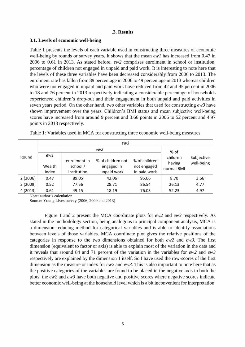
Table 1 presents the levels of each variable used in constructing three measures of economic
well-being by rounds or survey years. It shows that the mean ew1 has increased from 0.47 in
2006 to 0.61 in 2013. As stated before, ew2 comprises enrolment in school or institution,
percentage of children not engaged in unpaid and paid work. It is interesting to note here that
the levels of these three variables have been decreased considerably from 2006 to 2013. The
enrolment rate has fallen from 89 percentage in 2006 to 49 percentage in 2013 whereas children
who were not engaged in unpaid and paid work have reduced from 42 and 95 percent in 2006
to 18 and 76 percent in 2013 respectively indicating a considerable percentage of households
experienced children’s drop-out and their engagement in both unpaid and paid activities in
seven years period. On the other hand, two other variables that used for constructing ew3 have
shown improvement over the years. Children’s BMI status and mean subjective well-being
scores have increased from around 9 percent and 3.66 points in 2006 to 52 percent and 4.97
points in 2013 respectively.
Table 1: Variables used in MCA for constructing three economic well-being measures
Round
ew3
ew2 % of
children having
normal BMI
Subjective well-being
ew1
Wealth Index
enrolment in school /
institution
% of children not engaged in
unpaid work
% of children not engaged in paid work
2 (2006) 0.47 89.05 42.06 95.06 8.70 3.66
3 (2009) 0.52 77.56 28.71 86.54 26.13 4.77
4 (2013) 0.61 49.15 18.19 76.03 52.23 4.97 Note: author’s calculation
Source: Young Lives survey (2006, 2009 and 2013)
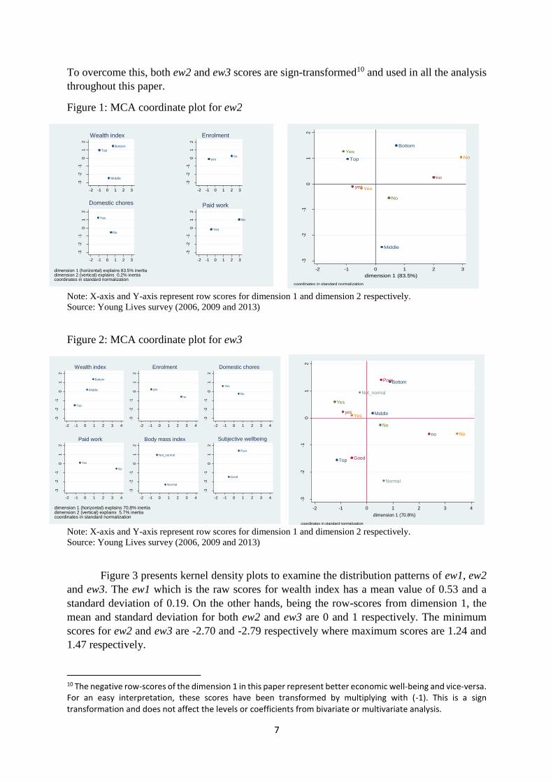
Figure 1 and 2 present the MCA coordinate plots for ew2 and ew3 respectively. As
stated in the methodology section, being analogous to principal component analysis, MCA is
a dimension reducing method for categorical variables and is able to identify associations
between levels of those variables. MCA coordinate plot gives the relative positions of the
categories in response to the two dimensions obtained for both ew2 and ew3. The first
dimension (equivalent to factor or axis) is able to explain most of the variation in the data and
it reveals that around 84 and 71 percent of the variation in the variables for ew2 and ew3
respectively are explained by the dimension 1 itself. So I have used the row-scores of the first
dimension as the measure or index for ew2 and ew3. This is also important to note here that as
the positive categories of the variables are found to be placed in the negative axis in both the
plots, the ew2 and ew3 have both negative and positive scores where negative scores indicate
better economic well-being at the household level which is a bit inconvenient for interpretation.
7
To overcome this, both ew2 and ew3 scores are sign-transformed10 and used in all the analysis
throughout this paper.
Figure 1: MCA coordinate plot for ew2
Note: X-axis and Y-axis represent row scores for dimension 1 and dimension 2 respectively.
Source: Young Lives survey (2006, 2009 and 2013)
Figure 2: MCA coordinate plot for ew3
Note: X-axis and Y-axis represent row scores for dimension 1 and dimension 2 respectively.
Source: Young Lives survey (2006, 2009 and 2013)
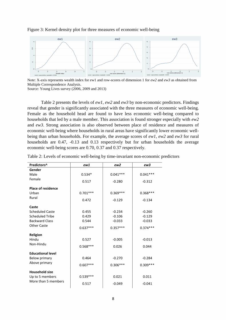
Figure 3 presents kernel density plots to examine the distribution patterns of ew1, ew2
and ew3. The ew1 which is the raw scores for wealth index has a mean value of 0.53 and a
standard deviation of 0.19. On the other hands, being the row-scores from dimension 1, the
mean and standard deviation for both ew2 and ew3 are 0 and 1 respectively. The minimum
scores for ew2 and ew3 are -2.70 and -2.79 respectively where maximum scores are 1.24 and
1.47 respectively.
10 The negative row-scores of the dimension 1 in this paper represent better economic well-being and vice-versa. For an easy interpretation, these scores have been transformed by multiplying with (-1). This is a sign transformation and does not affect the levels or coefficients from bivariate or multivariate analysis.
Bottom
Middle
Top
-3-2
-10
12
-2 -1 0 1 2 3
Wealth index
noyes
-3-2
-10
12
-2 -1 0 1 2 3
Enrolment
No
Yes
-3-2
-10
12
-2 -1 0 1 2 3
Domestic chores
No
Yes
-3-2
-10
12
-2 -1 0 1 2 3
Paid work
dimension 1 (horizontal) explains 83.5% inertiadimension 2 (vertical) explains 0.2% inertiacoordinates in standard normalization
Bottom
Middle
Top
no
yes
No
Yes
No
Yes
-3-2
-10
12
dim
ensi
on
2 (
0.2
%)
-2 -1 0 1 2 3
dimension 1 (83.5%)
coordinates in standard normalization
Bottom
Middle
Top
-3-2
-10
12
-2 -1 0 1 2 3 4
Wealth index
no
yes
-3-2
-10
12
-2 -1 0 1 2 3 4
Enrolment
No
Yes
-3-2
-10
12
-2 -1 0 1 2 3 4
Domestic chores
No
Yes
-3-2
-10
12
-2 -1 0 1 2 3 4
Paid work
Not_normal
Normal
-3-2
-10
12
-2 -1 0 1 2 3 4
Body mass index
Poor
Good
-3-2
-10
12
-2 -1 0 1 2 3 4
Subjective wellbeing
dimension 1 (horizontal) explains 70.8% inertiadimension 2 (vertical) explains 5.7% inertiacoordinates in standard normalization
Bottom
Middle
Top
no
yes
No
Yes
No
Yes
Not_normal
Normal
Poor
Good
-3-2
-10
12
dim
ensio
n 2
( 5
.7%
)
-2 -1 0 1 2 3 4
dimension 1 (70.8%)
coordinates in standard normalization
8
Figure 3: Kernel density plot for three measures of economic well-being
Note: X-axis represents wealth index for ew1 and row-scores of dimension 1 for ew2 and ew3 as obtained from
Multiple Correspondence Analysis.
Source: Young Lives survey (2006, 2009 and 2013)
Table 2 presents the levels of ew1, ew2 and ew3 by non-economic predictors. Findings
reveal that gender is significantly associated with the three measures of economic well-being.
Female as the household head are found to have less economic well-being compared to
households that led by a male member. This association is found stronger especially with ew2
and ew3. Strong association is also observed between place of residence and measures of
economic well-being where households in rural areas have significantly lower economic well-
being than urban households. For example, the average scores of ew1, ew2 and ew3 for rural
households are 0.47, -0.13 and 0.13 respectively but for urban households the average
economic well-being scores are 0.70, 0.37 and 0.37 respectively.
Table 2: Levels of economic well-being by time-invariant non-economic predictors
Predictors^ ew1 ew2 ew3
Gender
Male 0.534* 0.041*** 0.041*** Female
0.517 -0.280 -0.312
Place of residence Urban 0.701*** 0.369*** 0.368*** Rural
0.472 -0.129 -0.134
Caste Scheduled Caste 0.455 -0.234 -0.260 Scheduled Tribe 0.429 -0.106 -0.129 Backward Class 0.544 -0.033 -0.033 Other Caste
0.637*** 0.357*** 0.374***
Religion Hindu 0.527 -0.005 -0.013 Non-Hindu
0.568*** 0.026 0.044
Educational level Below primary 0.464 -0.270 -0.284 Above primary
0.607*** 0.306*** 0.309***
Household size Up to 5 members 0.539*** 0.021 0.011 More than 5 members
0.517 -0.049 -0.041
0.5
11.5
2
De
nsity
0 .2 .4 .6 .8 1
Wealth indexkernel = epanechnikov, bandwidth = 0.0500
ew1
0.1
.2.3
.4
De
nsity
-3 -2 -1 0 1 2
row score (dimension 1)kernel = epanechnikov, bandwidth = 0.6000
ew2
0.1
.2.3
.4.5
De
nsity
-3 -2 -1 0 1 2row scores (dimenson 1)
kernel = epanechnikov, bandwidth = 0.4000
ew3
9
Region Coastal Andhra 0.549*** 0.171*** 0.158*** Ryalaseema 0.530 -0.071 -0.096 Telangana 0.515 -0.087 -0.066
Note: author’s calculation
Source: Young Lives survey (2006, 2009 and 2013)
Significance level: *p < 0.1, **p < 0.05, ***p < 0.01.
^ One-way ANOVA has been carried out for caste and region to test the significant association with dependent
variables. For other predictors, t-test has been carried out.
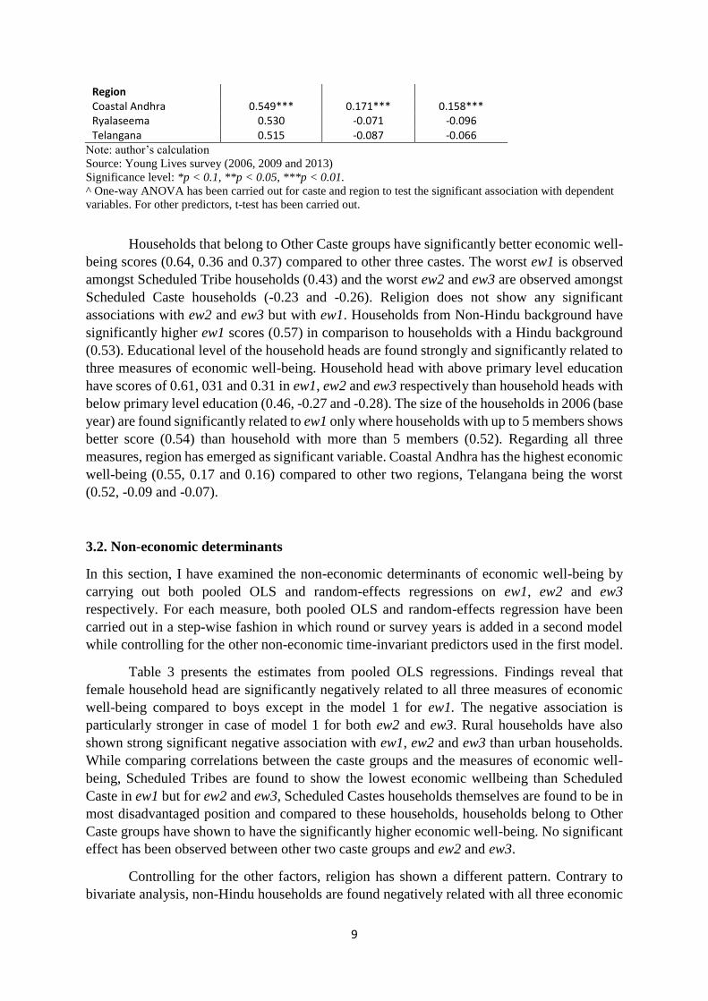
Households that belong to Other Caste groups have significantly better economic well-
being scores (0.64, 0.36 and 0.37) compared to other three castes. The worst ew1 is observed
amongst Scheduled Tribe households (0.43) and the worst ew2 and ew3 are observed amongst
Scheduled Caste households (-0.23 and -0.26). Religion does not show any significant
associations with ew2 and ew3 but with ew1. Households from Non-Hindu background have
significantly higher ew1 scores (0.57) in comparison to households with a Hindu background
(0.53). Educational level of the household heads are found strongly and significantly related to
three measures of economic well-being. Household head with above primary level education
have scores of 0.61, 031 and 0.31 in ew1, ew2 and ew3 respectively than household heads with
below primary level education (0.46, -0.27 and -0.28). The size of the households in 2006 (base
year) are found significantly related to ew1 only where households with up to 5 members shows
better score (0.54) than household with more than 5 members (0.52). Regarding all three
measures, region has emerged as significant variable. Coastal Andhra has the highest economic
well-being (0.55, 0.17 and 0.16) compared to other two regions, Telangana being the worst
(0.52, -0.09 and -0.07).
3.2. Non-economic determinants
In this section, I have examined the non-economic determinants of economic well-being by
carrying out both pooled OLS and random-effects regressions on ew1, ew2 and ew3
respectively. For each measure, both pooled OLS and random-effects regression have been
carried out in a step-wise fashion in which round or survey years is added in a second model
while controlling for the other non-economic time-invariant predictors used in the first model.
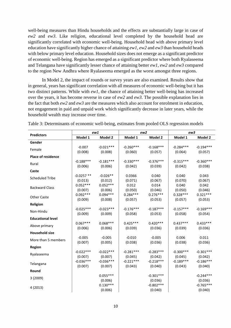
Table 3 presents the estimates from pooled OLS regressions. Findings reveal that
female household head are significantly negatively related to all three measures of economic
well-being compared to boys except in the model 1 for ew1. The negative association is
particularly stronger in case of model 1 for both ew2 and ew3. Rural households have also
shown strong significant negative association with ew1, ew2 and ew3 than urban households.
While comparing correlations between the caste groups and the measures of economic well-
being, Scheduled Tribes are found to show the lowest economic wellbeing than Scheduled
Caste in ew1 but for ew2 and ew3, Scheduled Castes households themselves are found to be in
most disadvantaged position and compared to these households, households belong to Other
Caste groups have shown to have the significantly higher economic well-being. No significant
effect has been observed between other two caste groups and ew2 and ew3.
Controlling for the other factors, religion has shown a different pattern. Contrary to
bivariate analysis, non-Hindu households are found negatively related with all three economic
10
well-being measures than Hindu households and the effects are substantially large in case of
ew2 and ew3. Like religion, educational level completed by the household head are
significantly correlated with economic well-being. Household head with above primary level
education have significantly higher chance of attaining ew1, ew2 and ew3 than household heads
with below primary level education. Household sizes does not emerge as a significant predictor
of economic well-being. Region has emerged as a significant predictor where both Ryalaseema
and Telangana have significantly lesser chance of attaining better ew1, ew2 and ew3 compared
to the region New Andhra where Ryalaseema emerged as the worst amongst three regions.
In Model 2, the impact of rounds or survey years are also examined. Results show that
in general, years has significant correlation with all measures of economic well-being but it has
two distinct patterns. While with ew1, the chance of attaining better well-being has increased
over the years, it has become reverse in case of ew2 and ew3. The possible explanation lies in
the fact that both ew2 and ew3 are the measures which also account for enrolment in education,
not engagement in paid and unpaid work which significantly decrease in later years, while the
household wealth may increase over time.
Table 3: Determinants of economic well-being, estimates from pooled OLS regression models
Predictors ew1 ew2 ew3
Model 1 Model 2 Model 1 Model 2 Model 1 Model 2
Gender
Female -0.007 (0.008)
-0.021*** (0.008)
-0.260*** (0.060)
-0.168*** (0.057)
-0.284*** (0.064)
-0.194*** (0.057)
Place of residence
Rural -0.188***
(0.006) -0.181***
(0.006) -0.330***
(0.042) -0.376***
(0.039) -0.315***
(0.042) -0.360***
(0.038) Caste
Scheduled Tribe -0.0257 **
(0.013) -0.026** (0.012)
0.0366 (0.071)
0.040 (0.067)
0.040 (0.070)
0.043 (0.067)
Backward Class 0.052*** (0.007)
0.052*** (0.006)
0.012 (0.050)
0.014 (0.046)
0.040 (0.050)
0.042 (0.046)
Other Caste 0.092*** (0.009)
0.094*** (0.008)
0.284*** (0.057)
0.276*** (0.053)
0.328*** (0.057)
0.321*** (0.053)
Religion
Non-Hindu -0.025***
(0.009) -0.023***
(0.009) -0.176***
(0.058) -0.187***
(0.053) -0.157***
(0.058) -0.169***
(0.054) Educational level
Above primary 0.067*** (0.006)
0.068*** (0.006)
0.425*** (0.039)
0.420*** (0.036)
0.437*** (0.039)
0.433*** (0.036)
Household size
More than 5 members -0.005 (0.007)
-0.005 (0.005)
-0.010 (0.038)
-0.005 (0.036)
0.006 (0.038)
0.011 (0.036)
Region
Ryalaseema -0.022***
(0.007) -0.022***
(0.007) -0.281***
(0.045) -0.283***
(0.042) -0.300***
(0.045) -0.301***
(0.042)
Telangana -0.036***
(0.007) -0.036***
(0.007) -0.221***
(0.043) -0.218***
(0.040) -0.189***
(0.043) -0.186***
(0.040) Round
3 (2009) 0.055*** (0.006)
-0.301***
(0.036)
-0.244*** (0.036)
4 (2013) 0.130*** (0.006)
-0.802***
(0.040)
-0.765*** (0.040)
11
Constant 0.623
(0.010) 0.557
(0.010) 0.206
(0.068) 0.595
(0.064) 0.152
(0.068) 0.510
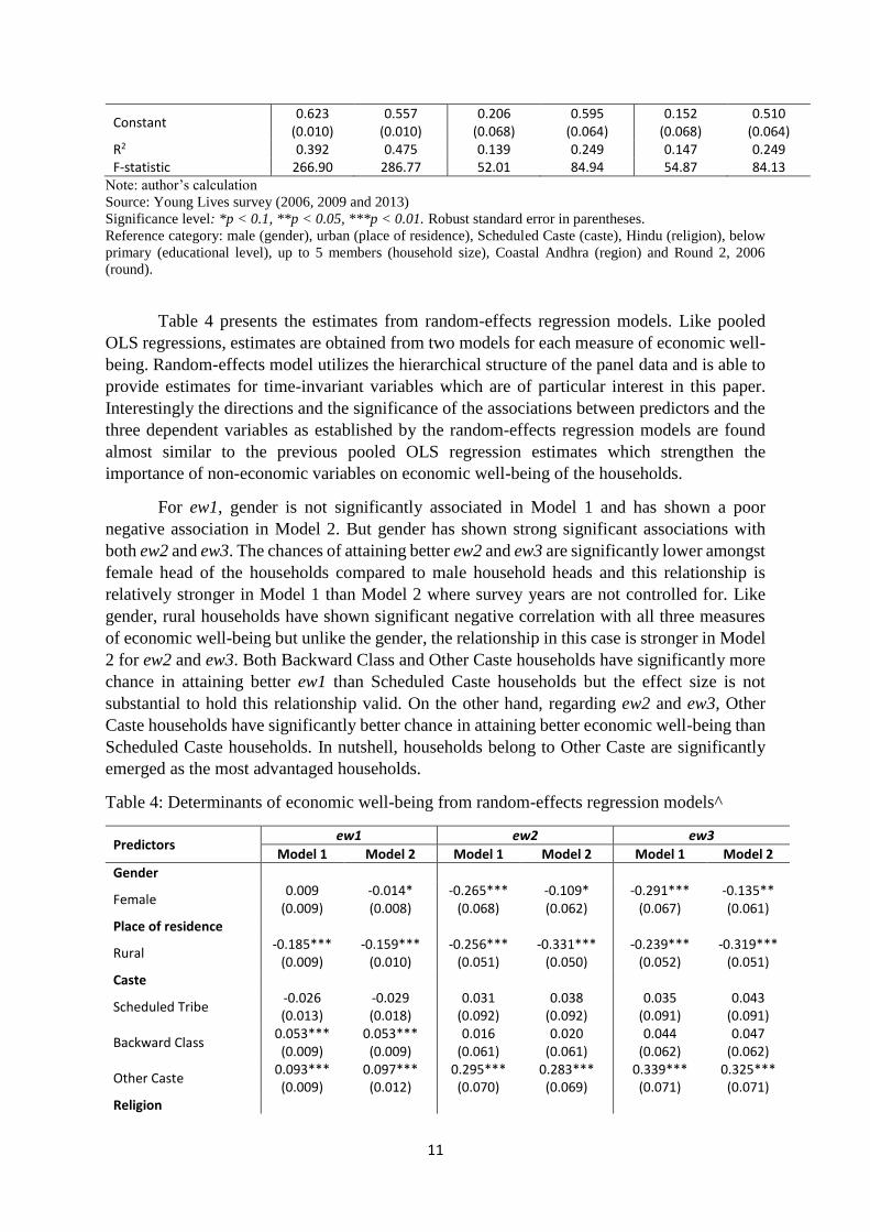
(0.064) R2 0.392 0.475 0.139 0.249 0.147 0.249 F-statistic 266.90 286.77 52.01 84.94 54.87 84.13
Note: author’s calculation
Source: Young Lives survey (2006, 2009 and 2013)
Significance level: *p < 0.1, **p < 0.05, ***p < 0.01. Robust standard error in parentheses.
Reference category: male (gender), urban (place of residence), Scheduled Caste (caste), Hindu (religion), below
primary (educational level), up to 5 members (household size), Coastal Andhra (region) and Round 2, 2006
(round).
Table 4 presents the estimates from random-effects regression models. Like pooled
OLS regressions, estimates are obtained from two models for each measure of economic well-
being. Random-effects model utilizes the hierarchical structure of the panel data and is able to
provide estimates for time-invariant variables which are of particular interest in this paper.
Interestingly the directions and the significance of the associations between predictors and the
three dependent variables as established by the random-effects regression models are found
almost similar to the previous pooled OLS regression estimates which strengthen the
importance of non-economic variables on economic well-being of the households.
For ew1, gender is not significantly associated in Model 1 and has shown a poor
negative association in Model 2. But gender has shown strong significant associations with
both ew2 and ew3. The chances of attaining better ew2 and ew3 are significantly lower amongst
female head of the households compared to male household heads and this relationship is
relatively stronger in Model 1 than Model 2 where survey years are not controlled for. Like
gender, rural households have shown significant negative correlation with all three measures
of economic well-being but unlike the gender, the relationship in this case is stronger in Model
2 for ew2 and ew3. Both Backward Class and Other Caste households have significantly more
chance in attaining better ew1 than Scheduled Caste households but the effect size is not
substantial to hold this relationship valid. On the other hand, regarding ew2 and ew3, Other
Caste households have significantly better chance in attaining better economic well-being than
Scheduled Caste households. In nutshell, households belong to Other Caste are significantly
emerged as the most advantaged households.
Table 4: Determinants of economic well-being from random-effects regression models^
Predictors ew1 ew2 ew3
Model 1 Model 2 Model 1 Model 2 Model 1 Model 2
Gender
Female 0.009
(0.009) -0.014* (0.008)
-0.265*** (0.068)
-0.109* (0.062)
-0.291*** (0.067)
-0.135** (0.061)
Place of residence
Rural -0.185***
(0.009) -0.159***
(0.010) -0.256***
(0.051) -0.331***
(0.050) -0.239***
(0.052) -0.319***
(0.051) Caste
Scheduled Tribe -0.026 (0.013)
-0.029 (0.018)
0.031 (0.092)
0.038 (0.092)
0.035 (0.091)
0.043 (0.091)
Backward Class 0.053*** (0.009)
0.053*** (0.009)
0.016 (0.061)
0.020 (0.061)
0.044 (0.062)
0.047 (0.062)
Other Caste 0.093*** (0.009)
0.097*** (0.012)
0.295*** (0.070)
0.283*** (0.069)
0.339*** (0.071)
0.325*** (0.071)
Religion
12
Non-Hindu -0.025** (0.013)
-0.019 (0.013)
-0.160** (0.070)
-0.179** (0.071)
-0.139** (0.071)
-0.159** (0.072)
Educational level
Above primary 0.069*** (0.009)
0.073*** (0.009)
0.440*** (0.048)
0.434*** (0.048)
0.452*** (0.049)
0.446*** (0.049)
Household size
More than 5 members -0.004 (0.008)
-0.005 (0.008)
-0.010 (0.048)
-0.001 (0.048)
0.005 (0.049)
0.014 (0.048)
Region
Ryalaseema -0.024** (0.009)
-0.026*** (0.009)
-0.282*** (0.055)
-0.279*** (0.054)
-0.298*** (0.055)
-0.294*** (0.055)
Telangana -0.034***
(0.009) -0.036***
(0.009) -0.223***
(0.054) -0.214***
(0.054) -0.193***
(0.054) -0.183***
(0.054) Round
3 (2009) 0.055*** (0.004)
-0.303***
(0.026)
-0.246*** (0.026)
4 (2013) 0.130*** (0.005)
-0.806***
(0.034)
-0.770*** (0.034)
Constant 0.616
(0.013) 0.537
(0.014) 0.139
(0.081) 0.539
(0.080) 0.083
(0.083) 0.456
(0.081) R2 - Within 0.057 0.371 0.001 0.262 0.003 0.255 R2- Between 0.502 0.508 0.238 0.239 0.242 0.244 R2- Overall 0.392 0.473 0.139 0.248 0.146 0.248
Note: author’s calculation
Source: Young Lives survey (2006, 2009 and 2013)
Significance level: *p < 0.1, **p < 0.05, ***p < 0.01. Robust standard error in parentheses.
Reference category: male (gender), urban (place of residence), Scheduled Caste (caste), Hindu (religion), below
primary (educational level), up to 5 members (household size), Coastal Andhra (region) and Round 2, 2006
(round).
^Lagrange multiplier (LM) test is carried out for each model to examine the validity of random-effects model over
pooled OLS regression and the significance level from each test validates the random-effects regression estimates
in this table.
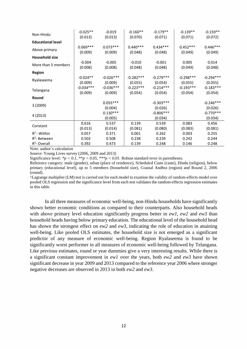
In all three measures of economic well-being, non-Hindu households have significantly
shown better economic conditions as compared to their counterparts. Also household heads
with above primary level education significantly progress better in ew1, ew2 and ew3 than
household heads having below primary education. The educational level of the household head
has shown the strongest effect on ew2 and ew3, indicating the role of education in attaining
well-being. Like pooled OLS estimates, the household size is not emerged as a significant
predictor of any measure of economic well-being. Region Ryalaseema is found to be
significantly worst performer in all measures of economic well-being followed by Telangana.
Like previous estimates, round or year dummies give a very interesting results. While there is
a significant constant improvement in ew1 over the years, both ew2 and ew3 have shown
significant decrease in year 2009 and 2013 compared to the reference year 2006 where stronger
negative decreases are observed in 2013 in both ew2 and ew3.
13
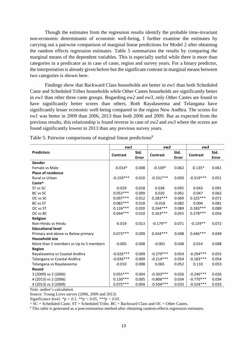
Though the estimates from the regression results identify the probable time-invariant
non-economic determinants of economic well-being, I further examine the estimates by
carrying out a pairwise comparison of marginal linear predictions for Model 2 after obtaining
the random effects regression estimates. Table 5 summarizes the results by comparing the
marginal means of the dependent variables. This is especially useful while there is more than
categories in a predicator as in case of caste, region and survey years. For a binary predictor,
the interpretation is already given before but the significant contrast in marginal means between
two categories is shown here.
Findings show that Backward Class households are better in ew1 than both Scheduled
Caste and Scheduled Tribes households while Other Castes households are significantly better
in ew1 than other three caste groups. Regarding ew2 and ew3, only Other Castes are found to
have significantly better scores than others. Both Rayalaseema and Telangana have
significantly lesser economic well-being compared to the region New Andhra. The scores for
ew1 was better in 2009 than 2006, 2013 than both 2006 and 2009. But as expected from the
previous results, this relationship is found reverse in case of ew2 and ew3 where the scores are
found significantly lowest in 2013 than any previous survey years.
Table 5: Pairwise comparisons of marginal linear predictions#
Predictors
ew1 ew2 ew3
Contrast Std. Error
Contrast Std. Error
Contrast Std. Error
Gender Female vs Male -0.014* 0.008 -0.109* 0.062 -0.135* 0.061 Place of residence Rural vs Urban -0.159*** 0.010 -0.331*** 0.050 -0.319*** 0.051 Caste^ ST vs SC -0.029 0.018 0.038 0.092 0.043 0.091 BC vs SC 0.053*** 0.009 0.020 0.061 0.047 0.062 OC vs SC 0.097*** 0.012 0.283*** 0.069 0.325*** 0.071 BC vs ST 0.082*** 0.018 -0.018 0.082 0.004 0.081 OC vs ST 0.126*** 0.020 0.244*** 0.089 0.283*** 0.089 OC vs BC 0.044*** 0.010 0.263*** 0.055 0.278*** 0.056 Religion Non-Hindu vs Hindu -0.019 0.013 -0.179** 0.071 -0.159** 0.072 Educational level Primary and above vs Below primary 0.073*** 0.009 0.434*** 0.048 0.446*** 0.049 Household size More than 5 members vs Up to 5 members -0.005 0.008 -0.001 0.048 0.014 0.048 Region Rayalaseema vs Coastal Andhra -0.026*** 0.009 -0.279*** 0.054 -0.294*** 0.055 Telangana vs Coastal Andhra -0.036*** 0.009 -0.214*** 0.054 -0.183*** 0.054 Telangana vs Rayalaseema -0.010 0.008 0.065 0.052 0.110 0.053 Round 3 (2009) vs 2 (2006) 0.055*** 0.004 -0.303*** 0.026 -0.246*** 0.026 4 (2013) vs 2 (2006) 0.130*** 0.005 -0.806*** 0.034 -0.770*** 0.034 4 (2013) vs 3 (2009) 0.075*** 0.004 -0.504*** 0.033 -0.524*** 0.033
Note: author’s calculation
Source: Young Lives survey (2006, 2009 and 2013)
Significance level: *p < 0.1, **p < 0.05, ***p < 0.01.
^ SC = Scheduled Caste, ST = Scheduled Tribe, BC = Backward Class and OC = Other Castes. # This table is generated as a post-estimation method after obtaining random-effects regression estimates.
14
4. Conclusion
Drawing on the experience of Young Lives, a longitudinal study of childhood poverty, this
paper makes an attempt to contribute to the study of economic well-being by analysing three
different measures. Along with the conventional wealth index; this paper also added other
economic and subjective variables in constructing the measures which are also dynamic and
sensitive to culture and time. As a result, the two constructed measures give a very different
picture of well-being from that of wealth index for some predictors.
First this paper argues for including non-conventional indicators of well-being in the
composite index building process that can represent overall economic conditions or well-being
at household level. This paper also shows the use of Multiple Correspondence Analysis to
construct the index while the indicator variables are categorical. This is particularly helpful as
many sample surveys collect categorical responses for some variables which may be relevant
in the context of economic well-being. For example, current enrolment status of a child at a
household gives hint on household’s economic situation, especially when collected from a
same household over the years. Illustratively, if no drop-out has been observed from a
household over the years, it would not be very unwise to consider that the household’s
economic status is relatively stable, at least regarding this particular child, given other factors
remain constant.
Using this logic, considering wealth index is the first measure of economic well-being,
this paper considers variables like enrolment status, and not engagement in unpaid and paid
activities along with wealth index to build a second measure that depicts a broader notion of
economic well-being. Further, health status and subjective well-being are added to the previous
measure to make the concept of economic well-being more realistic and holistic. Secondly
these measures are examined by time-invariant non-economic predictors which is very relevant
in case of India. The results thus obtained are very practical and hence proved useful.
Findings in general reveal that there are significant changes of economic well-being
over time and by predictors. Educational level (above primary), caste (Other Castes), religious
background (Hindu), place of residence (urban) and gender (male) of the household head are
found to be in significantly better position than their counterparts in terms of all three measures
of well-being but this association is especially stronger for other two composite measures when
other economic, health and subjective dimensions are taken into consideration. But when
considering with wealth alone the relationship is not that noticeable. These measures highlight
that economic development have a socio-demographic dimension in India which is still
persisting. Also the regional differentiations in economic well-being are clearly marked where
New Andhra is found to be in better position than other regions.
Considering the subjective and other economic dimensions in two measures of
economic well-being shows that over the years overall economic well-being have actually
decreased while the first measure, i.e., wealth index has shown significant increase over the
years. If we consider wealth alone for economic well-being, then it may appear that there is a
steady economic progress but a composite measures of economic well-being have shown that
there are needs of serious policy formulation must aimed at particular groups who are being
deprived of education, leisure, better health and sound subjective well-being over the years.
15
References
Abdi, H. and D. Valentin, “Multiple Correspondence Analysis,” In N. Salkind (Eds),
Encyclopaedia of Measurement and Statistics, Sage Knowledge, 2007.
Allin, P, “Measuring Wellbeing in Modern Societies,” in Peter Y. Chen and Cary L. Cooper
(eds), Work and Wellbeing: Wellbeing: A Complete Reference Guide, Volume III,
Imperial College London, United Kingdom, 2014.
Atkinson, A. B., E.H., “On the measurement of inequality”, Journal of Economic Theory, 2,
244-263, 1970.
Bell, A. and K. Jones, “Explaining fixed effects: random effects modelling of time-series cross-
sectional and panel data,” Political Science Research and Methods, 3, 133–153, 2014.
Cohen, E. H., “Multi-dimensional analysis of international social indicators – education,
economy, media and demography”, Social Indicators Research, 50, 83–106, 2000.
Costa, P.S., N. C. Santos, P. Cunha, J. Cotter, and N. Sousa, “The use of multiple
correspondence analysis to explore associations between categories of qualitative
variables in healthy ageing”, Journal of Aging Research, Article ID 302163, 2013.
Hallerod, B. and D. Selden, “The Multi-dimensional characteristics of wellbeing: how different
aspects of wellbeing interact and do not interact with each other” Social Indicator
Research, 113, 807–825, 2013.
Haq, R. and U. Zia, “Multidimensional wellbeing: an index of quality of life in a developing
economy”, Social Indicators Research, 114, 997-1012, 2013.
Hawkins, J., “The four approaches to measuring wellbeing, In A. Podger and D. Trewin (Eds),
Measuring and Promoting Wellbeing: How Important is Economic Growth?, ANU
Press, 2014.
http://library.bsl.org.au/jspui/bitstream/1/1267/1/Measurement_of_economic_perform
ance_and_social_progress.pdf
Levy. S. and L. Guttman, L., “On the multivariate structure of wellbeing”, Social Indicators
Research, 2, 361-388, 1975.
Murias, P. F. Martinez and C. Miguel, “An economic wellbeing index for the Spanish
provinces: a data envelopment analysis approach,” Social Indicator Research, 77, 395–
417, 2006.
Ray, D., Development Economics, Oxford University Press, New Delhi, 2012.
Schimmack, U., J. Schupp, J., and G. G. Wagner, “The influence of environment and
personality on the affective and cognitive component of subjective wellbeing,” Social
Indicators Research, 89, 41–60, 2008.
16
Sen, A., Commodities and Capabilities, Oxford University Press, New Delhi, 1999.
Stiglitz, J. E., A. Sen, and J. Fitoussi, Report of the Commission on the Measurement of
Economic Performance and Social Progress, 2009.
Torres-Reyna, O., Panel Data Analysis Fixed and Random Effects using Stata (v. 4.2),
Princeton University, 2007. http://dss.princeton.edu/training/Panel101.pdf
White, S. C., “Analysing wellbeing: a framework for development practice,” Development in
Practice, 20, 158-172, 2010.
World Health Organisation (WHO), BMI Classification, 2016.
http://apps.who.int/bmi/index.jsp?introPage=intro_3.html