measures of significance jim linnemann michigan state university u. toronto dec 4, 2003
TRANSCRIPT
Measures of Significance
Jim Linnemann
Michigan State University
U. Toronto
Dec 4, 2003
A Prickly Problemnot to everyone’s taste…
• What is Significance?• Li and Ma Equations• Frequentist Methods• Bayesian Methods• Is Significance well-defined?• To Do• Help Wanted• Summary
A simple problemwith lots of answers…
• Two Poisson measurements– 1) “background region”– 2) “signal region” – Poisson assumptions usually well satisfied
• Is the 2nd measurement predicted by the first?1) Measure significance of failure of prediction:
Did I see something potentially interesting? I.e., not background
2) If “significant enough”proceed to estimation of size of new effect
I’ll describe practice in High Energy Physics and Gamma Ray Astronomy (Behavioral Statistics)
Crossed Disciplines…
To physicists, this may sound like a statistics talkOr both HEP and Astrophysics (or neither…)
To statisticians…a physics talk
Apologies, but I’m try trying to cross boundaries
What a sabbatical is for, no?
From HEP (D0 experiment) Working on Gamma Ray Astronomy (Milagro experiment)
Help?
• To my statistical colleagues:– Better understand Fraser-Reid with nuisance parameters
prime motive for visit• Geometrical intuition for nuisance parameters
– Is the indeterminacy of Z well understood?
– Binomial-Bayes identity interesting?
– Is Binomial test really best?
My Original GoalWhat Can HEP and Astrophysics Practice
Teach Each Other?Astrophysics (especially ray)
aims at simple formulae (very fast)calculates σ’s directly (Asymptotic Normal)hope it’s a good formula
HEP (especially Fermilab practice)
calculates probabilities by MC (general; slow)translates into σ’s for communication
loses track of analytic structureStatistics: what can I learn
This is a progress report…
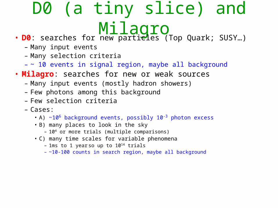
D0 (a tiny slice) and Milagro • D0: searches for new particles (Top Quark; SUSY…)
– Many input events– Many selection criteria– ~ 10 events in signal region, maybe all background
• Milagro: searches for new or weak sources– Many input events (mostly hadron showers)– Few photons among this background– Few selection criteria– Cases:
• A) ~106 background events, possibly 10-3 photon excess• B) many places to look in the sky
– 104 or more trials (multiple comparisons)
• C) many time scales for variable phenomena– 1ms to 1 year so up to 1014 trials– ~10-100 counts in search region, maybe all background
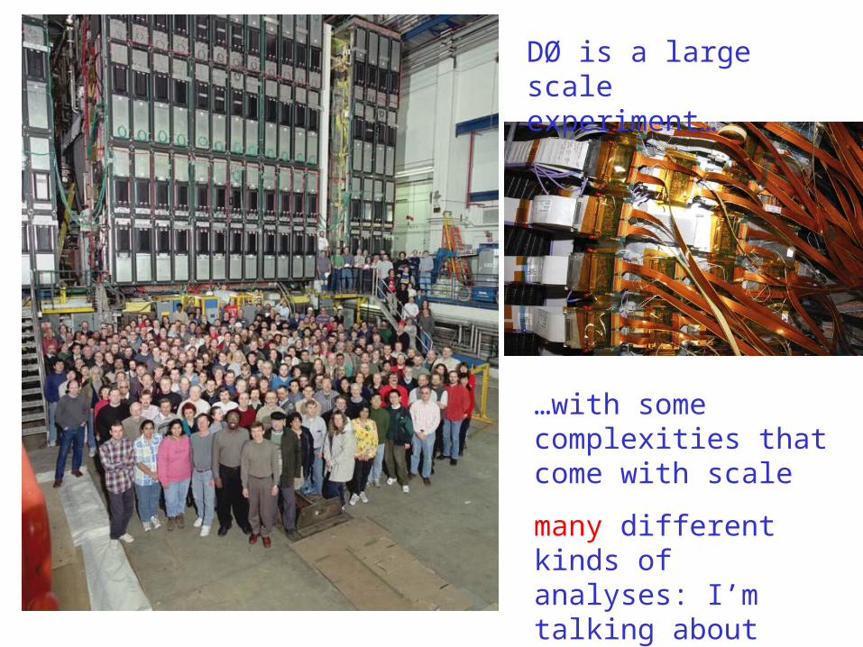
DØ is a large scale experiment…
…with some complexities that come with scale
many different kinds of analyses: I’m talking about searches only!
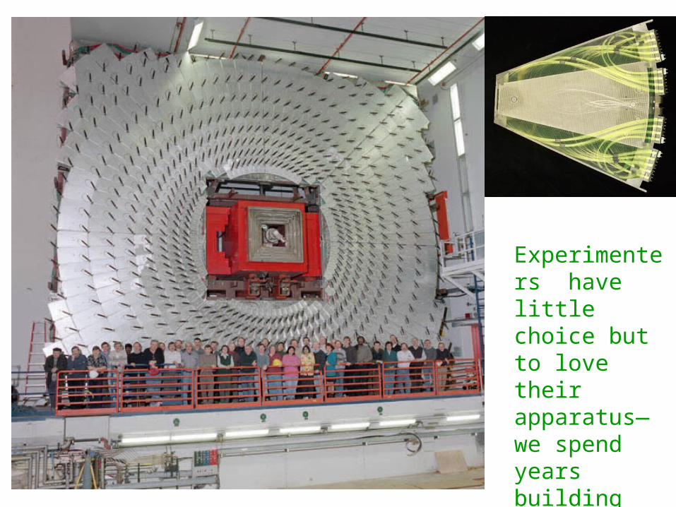
Experimenters have little choice but to love their apparatus—we spend years building it!
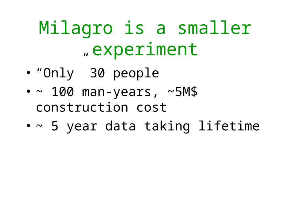
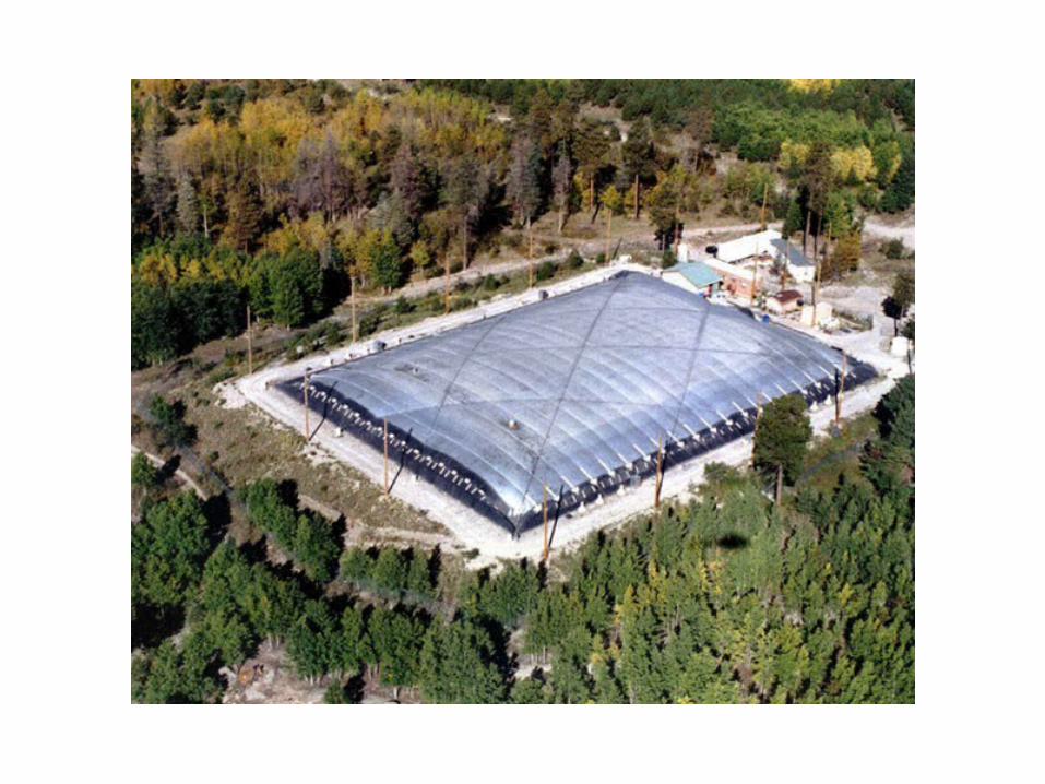
Milagro is a smaller experiment
• “Only” 30 people
• ~ 100 man-years, ~5M$ construction cost
• ~ 5 year data taking lifetime
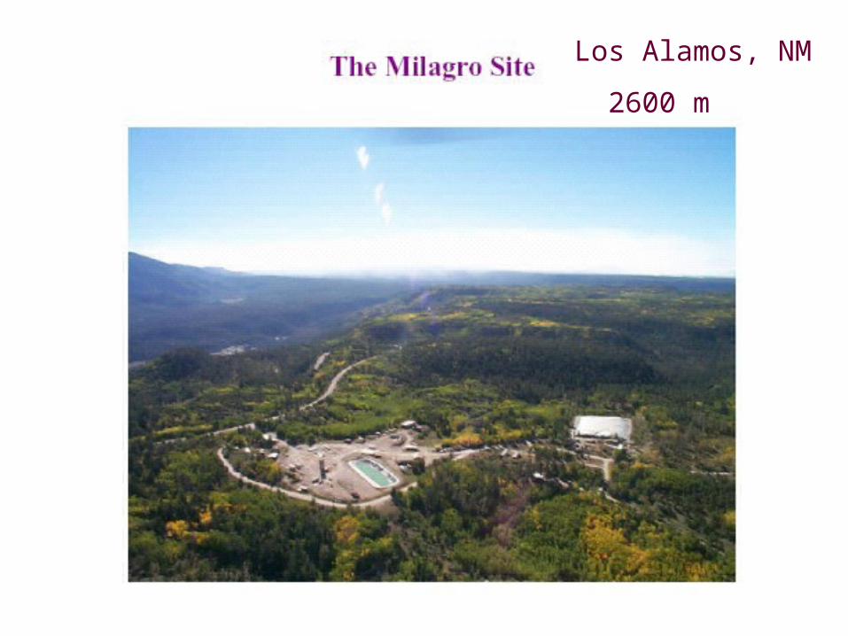
Los Alamos, NM
2600 m
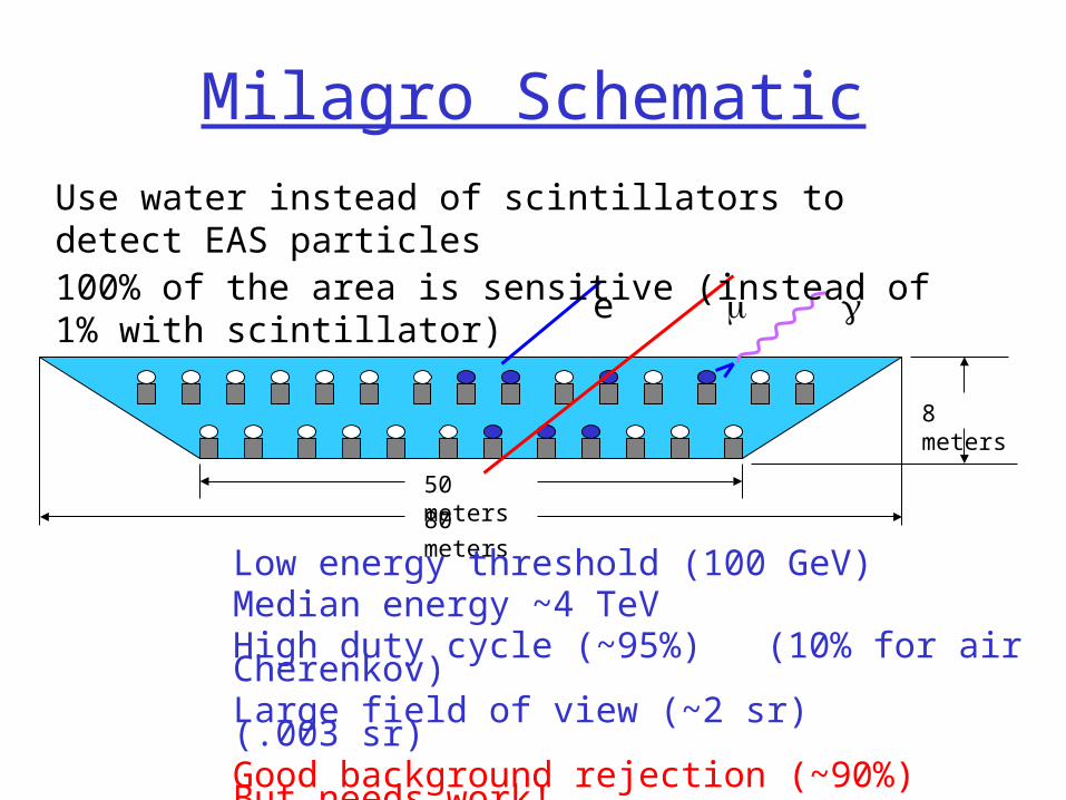
Milagro Schematic
8 meters
e
80 meters
50 meters
Use water instead of scintillators to detect EAS particles100% of the area is sensitive (instead of 1% with scintillator)
Low energy threshold (100 GeV)Median energy ~4 TeVHigh duty cycle (~95%) (10% for air Cherenkov)Large field of view (~2 sr) (.003 sr)Good background rejection (~90%) But needs work!Trigger Rate 1.7 kHz
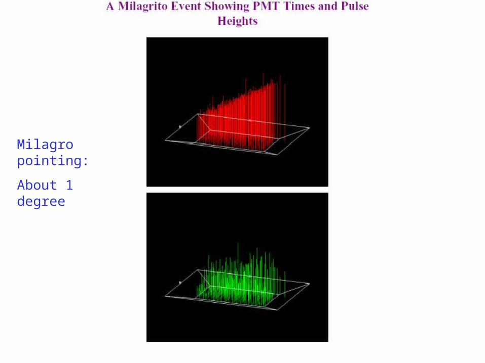
Milagro pointing:
About 1 degree
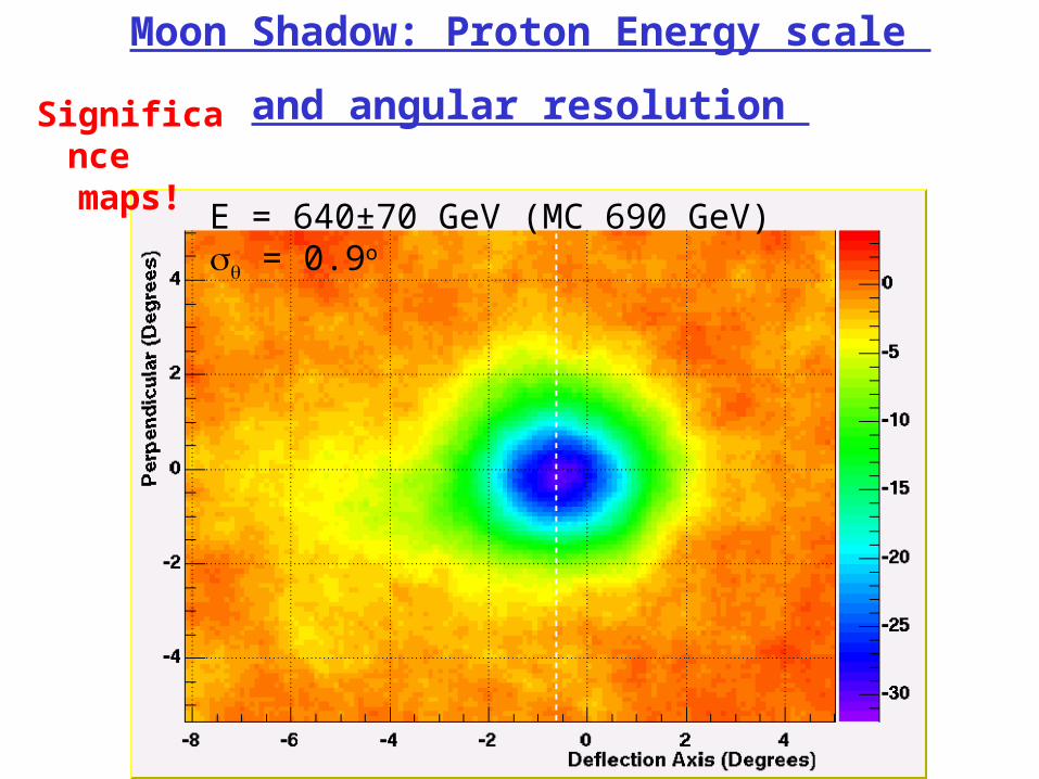
Moon Shadow: Proton Energy scale
and angular resolution
E = 640±70 GeV (MC 690 GeV) = 0.9o
Significance
maps!
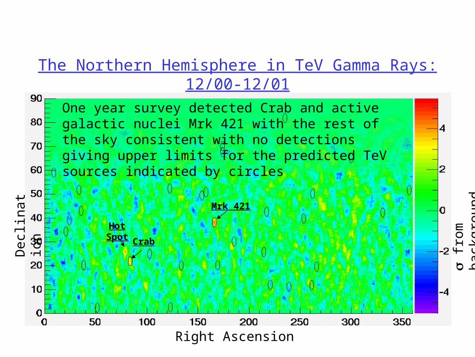
The Northern Hemisphere in TeV Gamma Rays: 12/00-12/01
Mrk 421
Crab
Hot Spot
De
clin
atio
n
Right Ascension
fr
om
b
ackg
rou
nd
One year survey detected Crab and active galactic nuclei Mrk 421 with the rest of the sky consistent with no detections giving upper limits for the predicted TeV sources indicated by circles
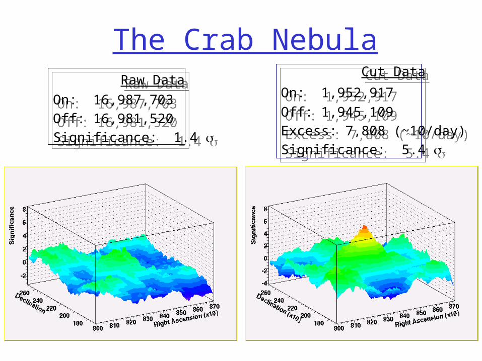
The Crab Nebula Raw Data
On: 16,987,703
Off: 16,981,520
Significance: 1.4
Raw Data
On: 16,987,703
Off: 16,981,520
Significance: 1.4
Cut Data
On: 1,952,917
Off: 1,945,109
Excess: 7,808 (~10/day)
Significance: 5.4
Cut Data
On: 1,952,917
Off: 1,945,109
Excess: 7,808 (~10/day)
Significance: 5.4
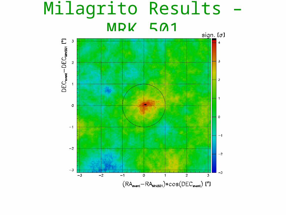
Milagrito Results – MRK 501
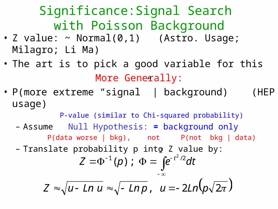
Significance:Signal Search with Poisson Background
• Z value: ~ Normal(0,1) (Astro. Usage; Milagro; Li Ma)• The art is to pick a good variable for this
More Generally:• P(more extreme “signal” | background) (HEP usage)
P-value (similar to Chi-squared probability)
– Assume Null Hypothesis: = background onlyP(data worse | bkg), not P(not bkg | data)
– Translate probability p into Z value by:
22,
);( 2/1 2
pLnupLnuLnuZ
dtepZZ
t
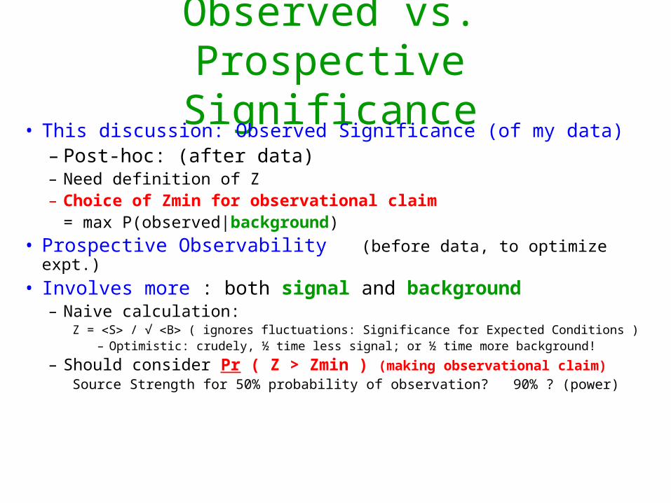
Observed vs. Prospective Significance
• This discussion: Observed Significance (of my data)– Post-hoc: (after data)– Need definition of Z– Choice of Zmin for observational claim
= max P(observed|background)
• Prospective Observability (before data, to optimize expt.)
• Involves more : both signal and background– Naive calculation:
Z = S / √ B ( ignores fluctuations: Significance for Expected Conditions )– Optimistic: crudely, ½ time less signal; or ½ time more background!
– Should consider Pr ( Z > Zmin ) (making observational claim)Source Strength for 50% probability of observation? 90% ? (power)
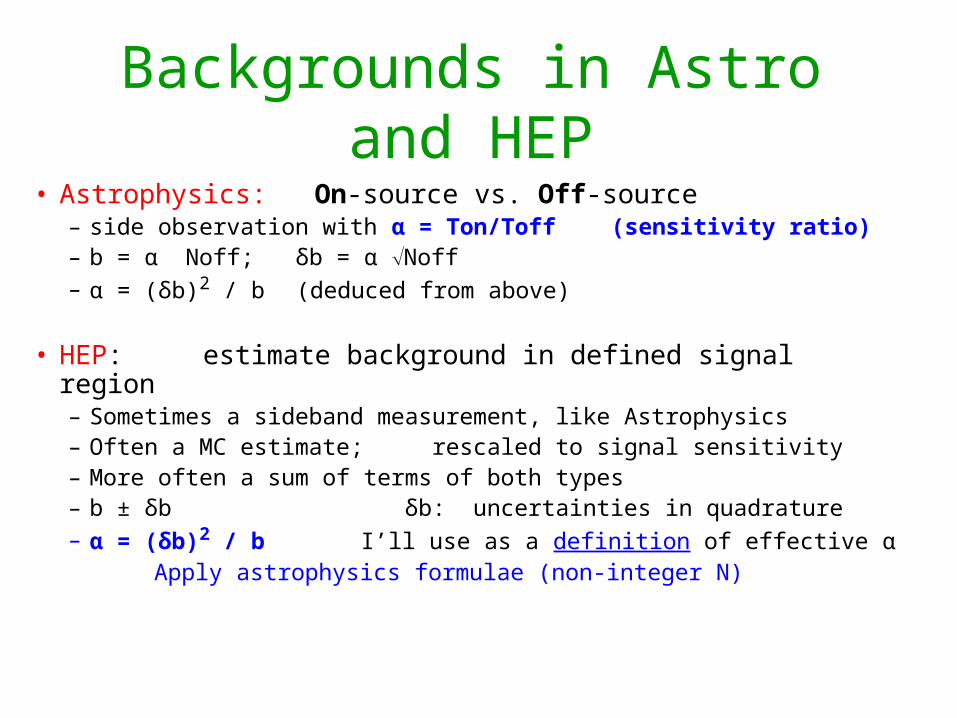
Backgrounds in Astro and HEP
• Astrophysics: On-source vs. Off-source– side observation with α = Ton/Toff (sensitivity ratio)– b = α Noff; δb = α Noff – α = (δb)2 / b (deduced from above)
• HEP: estimate background in defined signal region– Sometimes a sideband measurement, like Astrophysics– Often a MC estimate; rescaled to signal sensitivity– More often a sum of terms of both types– b ± δb δb: uncertainties in quadrature– α = (δb)2 / b I’ll use as a definition of effective α
Apply astrophysics formulae (non-integer N)
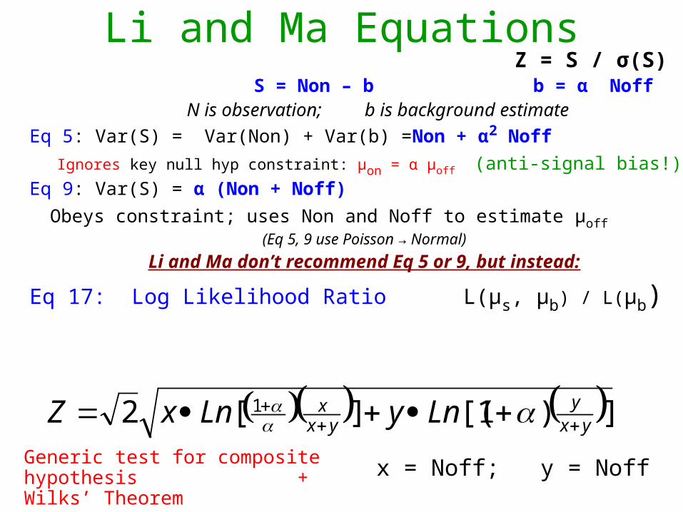
Li and Ma Equations Z = S / σ(S)
S = Non – b b = α NoffN is observation; b is background estimate
Eq 5: Var(S) = Var(Non) + Var(b) =Non + α2 Noff
Ignores key null hyp constraint: μon = α μoff (anti-signal bias!)
Eq 9: Var(S) = α (Non + Noff)
Obeys constraint; uses Non and Noff to estimate μoff(Eq 5, 9 use Poisson → Normal)
Li and Ma don’t recommend Eq 5 or 9, but instead:
Eq 17: Log Likelihood Ratio L(μs, μb) / L(μb)
])1[(][2 1yx
yyx
x LnyLnxZ
x = Noff; y = NoffGeneric test for composite hypothesis + Wilks’ Theorem
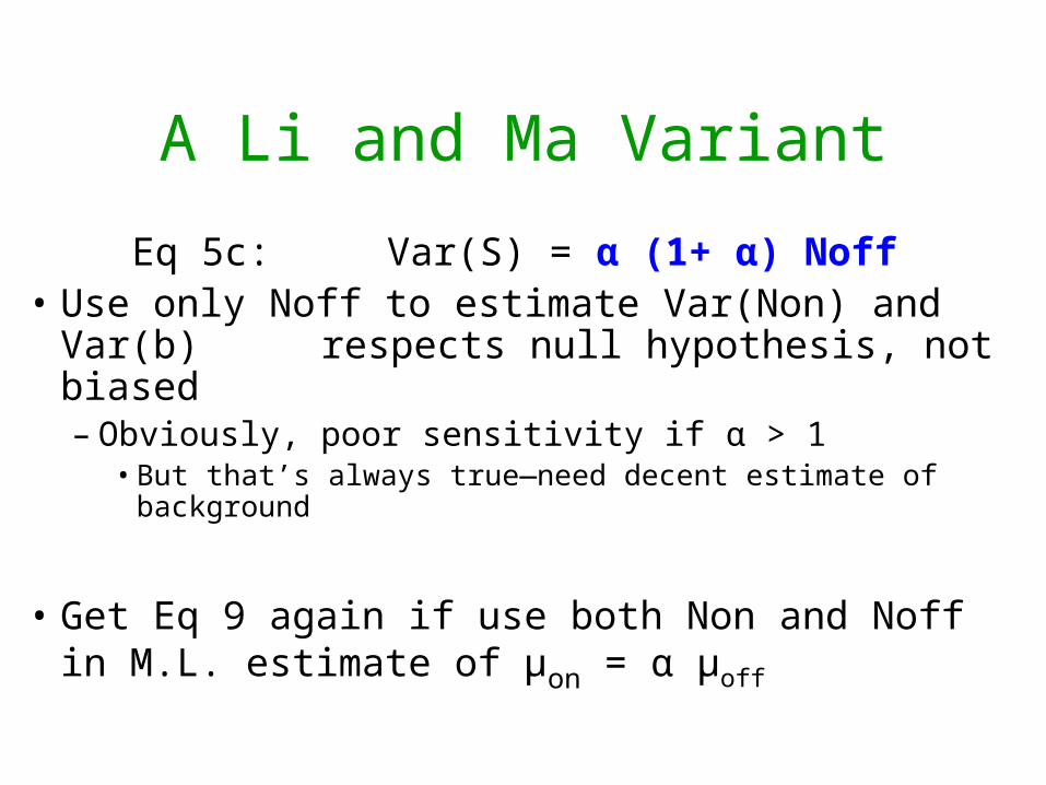
A Li and Ma Variant
Eq 5c: Var(S) = α (1+ α) Noff• Use only Noff to estimate Var(Non) and Var(b)
respects null hypothesis, not biased– Obviously, poor sensitivity if α > 1
• But that’s always true—need decent estimate of background
• Get Eq 9 again if use both Non and Noff in M.L. estimate of μon = α μoff
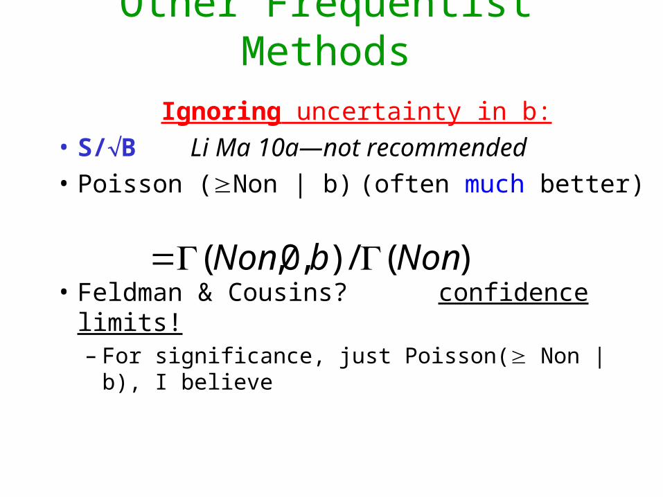
Other Frequentist Methods
Ignoring uncertainty in b:
• S/B Li Ma 10a—not recommended
• Poisson (Non | b) (often much better)
• Feldman & Cousins? confidence limits!– For significance, just Poisson( Non | b), I believe
)(/),0,( NonbNon
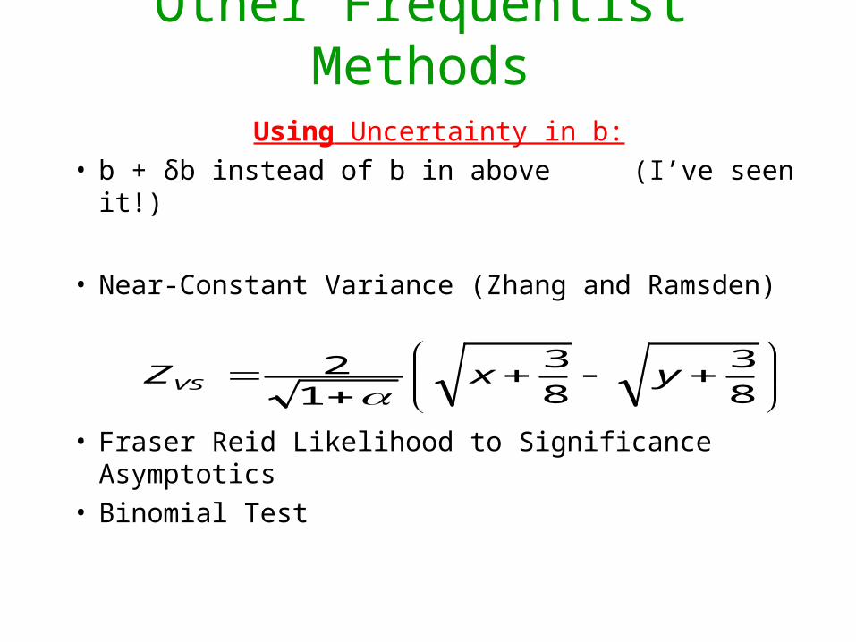
Other Frequentist Methods
Using Uncertainty in b:• b + δb instead of b in above (I’ve seen it!)
• Near-Constant Variance (Zhang and Ramsden)
• Fraser Reid Likelihood to Significance Asymptotics• Binomial Test
8
3
8
3
12 yxZVS
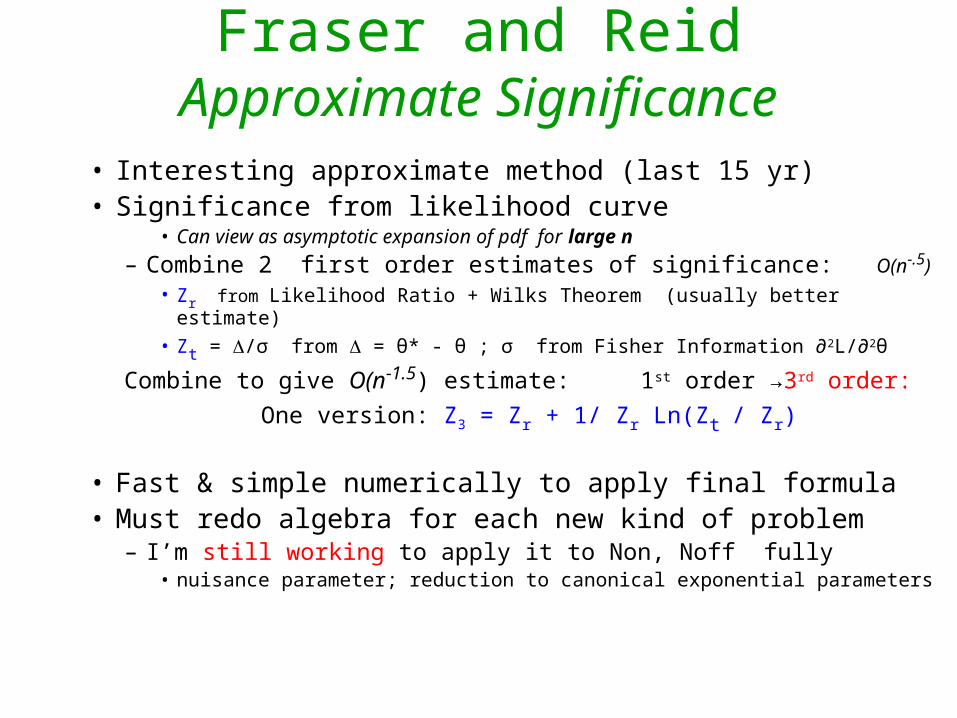
Fraser and ReidApproximate Significance
• Interesting approximate method (last 15 yr)• Significance from likelihood curve
• Can view as asymptotic expansion of pdf for large n
– Combine 2 first order estimates of significance: O(n-.5)
• Zr from Likelihood Ratio + Wilks Theorem (usually better estimate)
• Zt = /σ from = θ* - θ ; σ from Fisher Information ∂2L/∂2θ
Combine to give O(n-1.5) estimate: 1st order →3rd order:
One version: Z3 = Zr + 1/ Zr Ln(Zt / Zr)
• Fast & simple numerically to apply final formula • Must redo algebra for each new kind of problem
– I’m still working to apply it to Non, Noff fully • nuisance parameter; reduction to canonical exponential parameters
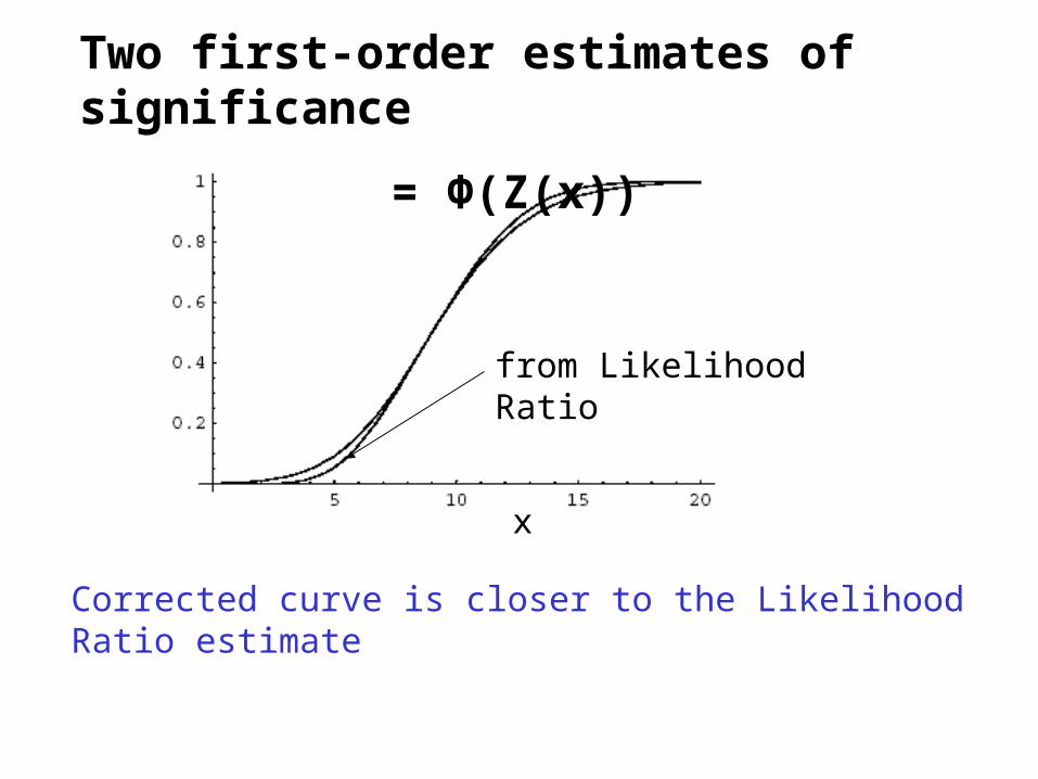
Two first-order estimates of significance
= Φ(Z(x))
from Likelihood Ratio
Corrected curve is closer to the Likelihood Ratio estimate
x
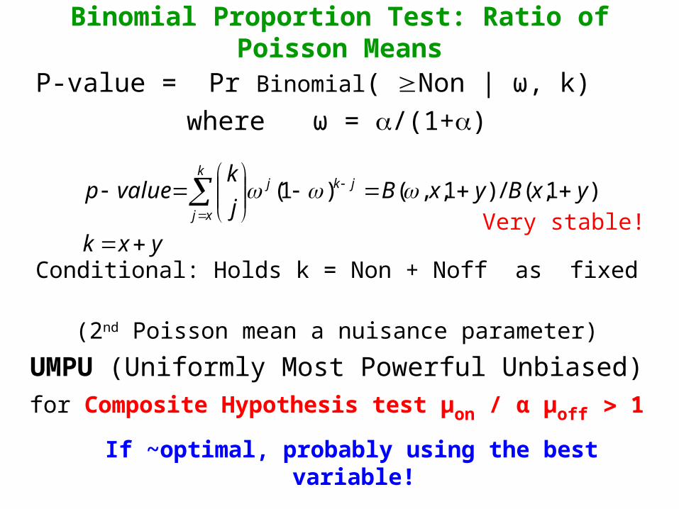
Binomial Proportion Test: Ratio of Poisson Means
P-value = Pr Binomial( Non | ω, k)
where ω = /(1+)
Conditional: Holds k = Non + Noff as fixed
(2nd Poisson mean a nuisance parameter)
UMPU (Uniformly Most Powerful Unbiased)
for Composite Hypothesis test μon / α μoff 1
If ~optimal, probably using the best variable!
yxk
yxByxBj
kvaluep jkj
k
xj
)1,(/)1,,()1(
Very stable!
Binomial Proportion Test: Ratio of Poisson Means
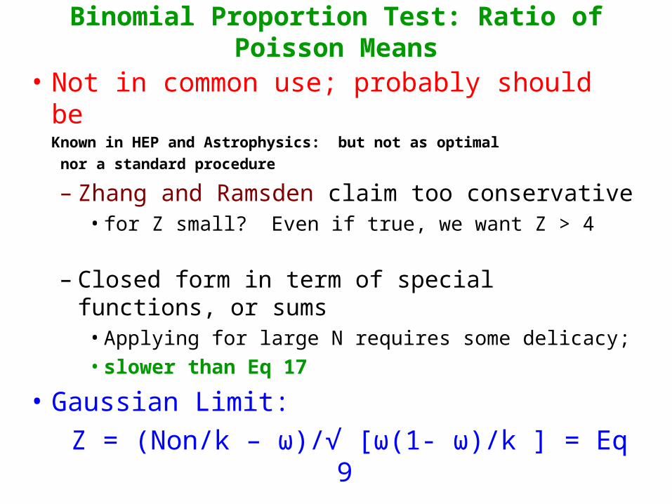
• Not in common use; probably should beKnown in HEP and Astrophysics: but not as optimal
nor a standard procedure
– Zhang and Ramsden claim too conservative • for Z small? Even if true, we want Z > 4
– Closed form in term of special functions, or sums• Applying for large N requires some delicacy;
• slower than Eq 17
• Gaussian Limit:
Z = (Non/k – ω)/√ [ω(1- ω)/k ] = Eq 9
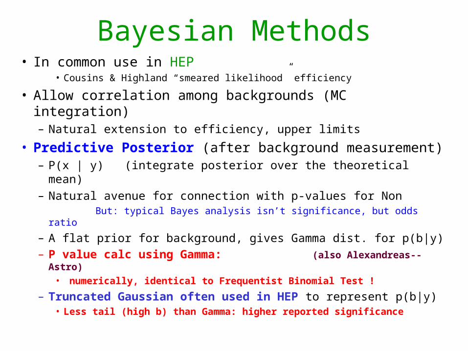
Bayesian Methods• In common use in HEP
• Cousins & Highland “smeared likelihood” efficiency
• Allow correlation among backgrounds (MC integration)– Natural extension to efficiency, upper limits
• Predictive Posterior (after background measurement)– P(x | y) (integrate posterior over the theoretical mean)
– Natural avenue for connection with p-values for Non But: typical Bayes analysis isn’t significance, but odds
ratio
– A flat prior for background, gives Gamma dist. for p(b|y)– P value calc using Gamma: (also Alexandreas--Astro)
• numerically, identical to Frequentist Binomial Test !
– Truncated Gaussian often used in HEP to represent p(b|y)• Less tail (high b) than Gamma: higher reported significance
Predictive Posterior Bayes P-value (HEP)
)|(),(
],/)([)|(
/,!
)|(
!)|(
)|()|()|(
yjpyxvalueP
ybbbNormalyp
y
eyp
j
ejp
dypjpyjp
xj
N
y
j
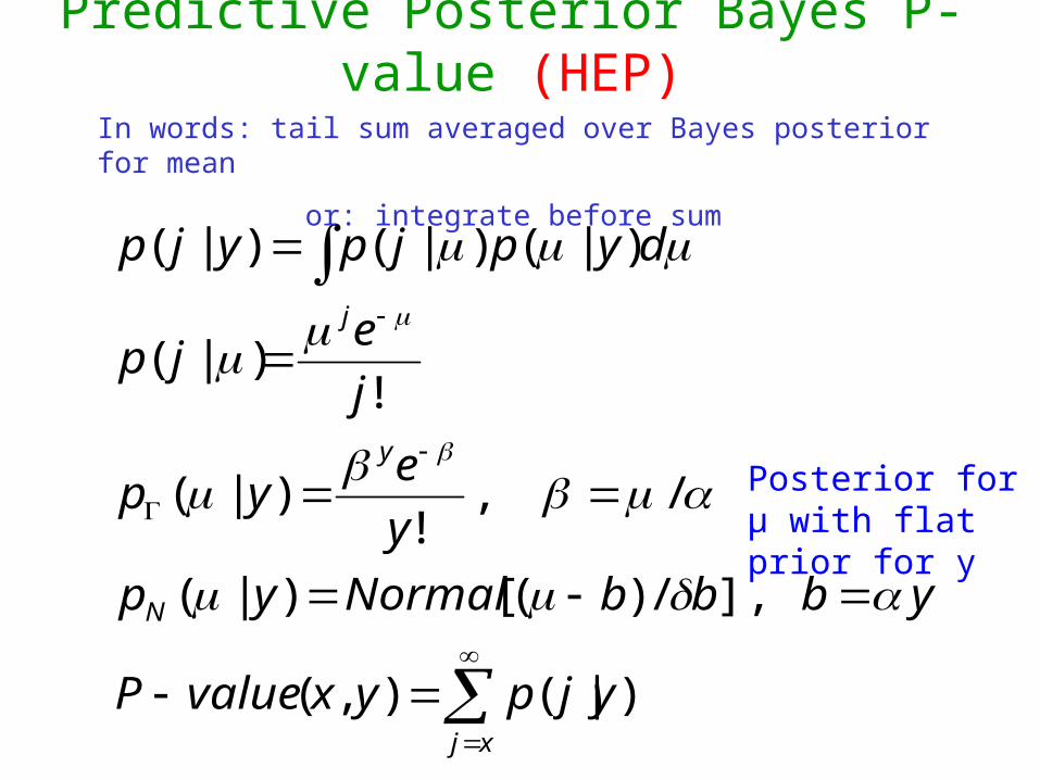
In words: tail sum averaged over Bayes posterior for mean
or: integrate before sum
Posterior for μ with flat prior for y
Two ways to write Bayesian p-value:
)|()|(
)|()|()|(),(
)|()|()|(
xjvaluepPoissonxjpwhere
dypxjpyjpyxvalueP
dypjpyjp
xj
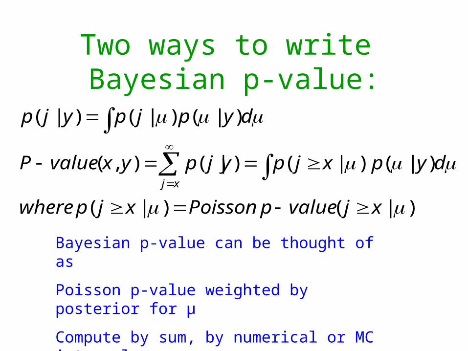
Bayesian p-value can be thought of as
Poisson p-value weighted by posterior for μ
Compute by sum, by numerical or MC integral
or, as it turns out, by an equivalent formula…
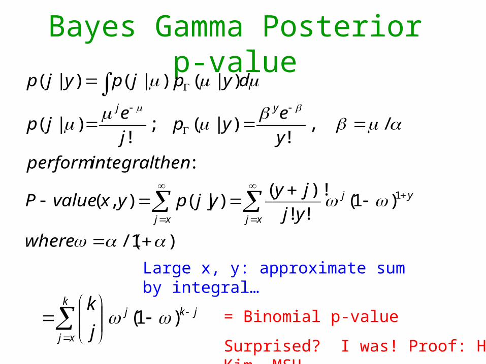
Bayes Gamma Posterior p-value
)1/(
)1(!!
)!()|(),(
:
/,!
)|(;!
)|(
)|()|()|(
1
where
yj
jyyjpyxvalueP
thenintegralperform
y
eyp
j
ejp
dypjpyjp
yj
xjxj
yj
Large x, y: approximate sum by integral…
jkjk
xj j
k
)1( = Binomial p-value
Surprised? I was! Proof: H. Kim, MSU
Comparing the Methods
• Some test cases from published literature• And a few artificial cases
– Range of Non, Noff values– Different α values (mostly < 1)– Interest: Z > 3, but sometimes >> 3 (many trials…)
• Color Code Accuracy – Assume Frequentist Binomial as Gold Standard
• Zhang and Ramsden found best supported by MCAt least when calculating Z > 3 or so
At worst, ZMC 3% higher

N increasing →
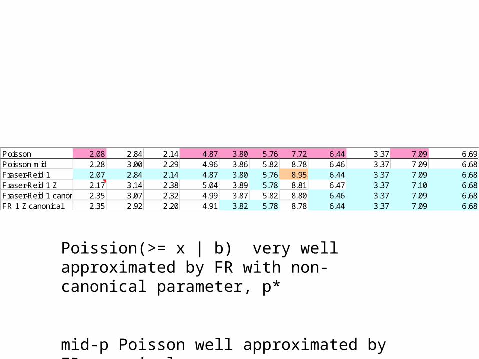
Poisson 2.08 2.84 2.14 4.87 3.80 5.76 7.72 6.44 3.37 7.09 6.69Poisson mid 2.28 3.00 2.29 4.96 3.86 5.82 8.78 6.46 3.37 7.09 6.68Fraser-Reid 1 2.07 2.84 2.14 4.87 3.80 5.76 8.95 6.44 3.37 7.09 6.68Fraser-Reid 1 Z 2.17 3.14 2.38 5.04 3.89 5.78 8.81 6.47 3.37 7.10 6.68Fraser-Reid 1 canonical 2.35 3.07 2.32 4.99 3.87 5.82 8.80 6.46 3.37 7.09 6.68FR 1 Z canonical 2.35 2.92 2.20 4.91 3.82 5.78 8.78 6.44 3.37 7.09 6.68
Poission(>= x | b) very well approximated by FR with non-canonical parameter, p*
mid-p Poisson well approximated by FR canonical,
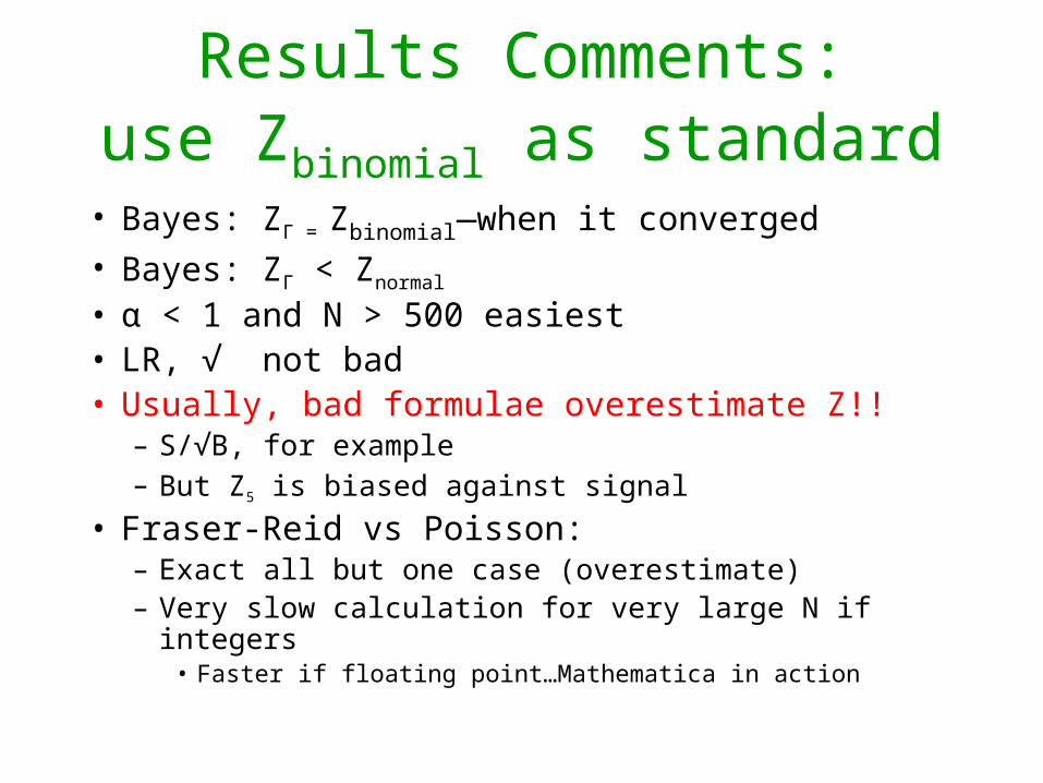
Results Comments:use Zbinomial as standard
• Bayes: ZΓ = Zbinomial—when it converged
• Bayes: ZΓ < Znormal
• α < 1 and N > 500 easiest• LR, √ not bad• Usually, bad formulae overestimate Z!!
– S/√B, for example– But Z5 is biased against signal
• Fraser-Reid vs Poisson:– Exact all but one case (overestimate)– Very slow calculation for very large N if integers
• Faster if floating point…Mathematica in action
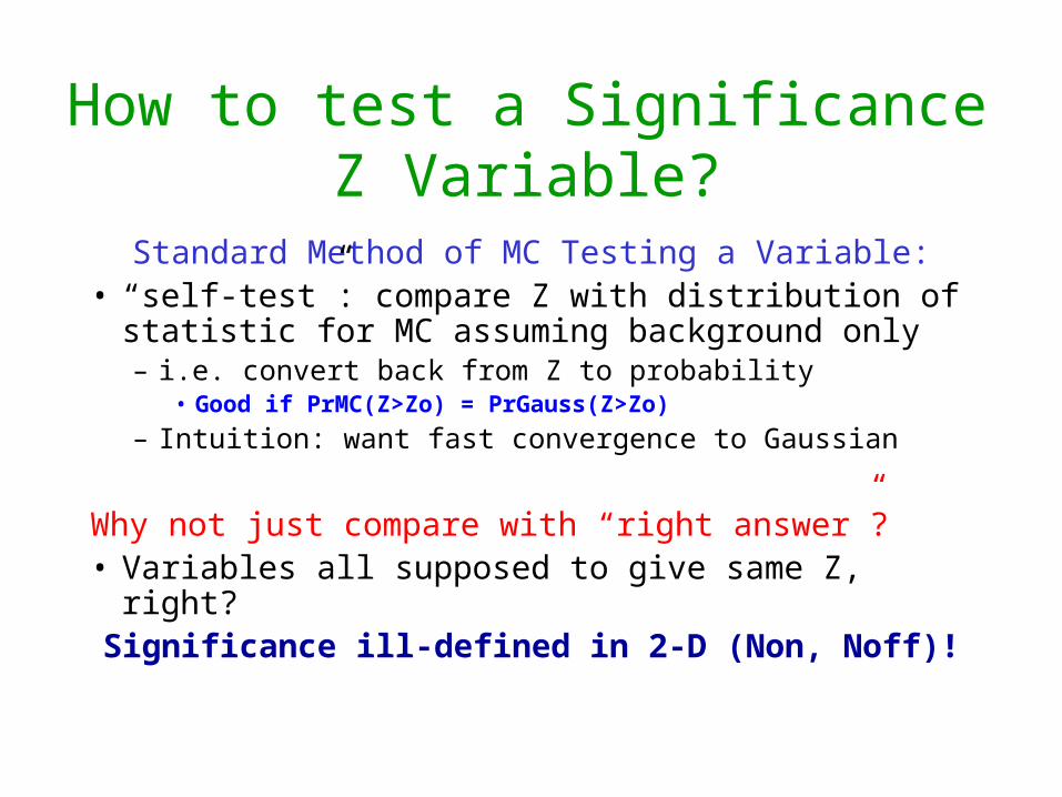
How to test a Significance Z Variable?
Standard Method of MC Testing a Variable:• “self-test”: compare Z with distribution of statistic for
MC assuming background only– i.e. convert back from Z to probability
• Good if PrMC(Z>Zo) = PrGauss(Z>Zo)
– Intuition: want fast convergence to Gaussian
Why not just compare with “right answer”?• Variables all supposed to give same Z, right?
Significance ill-defined in 2-D (Non, Noff)!
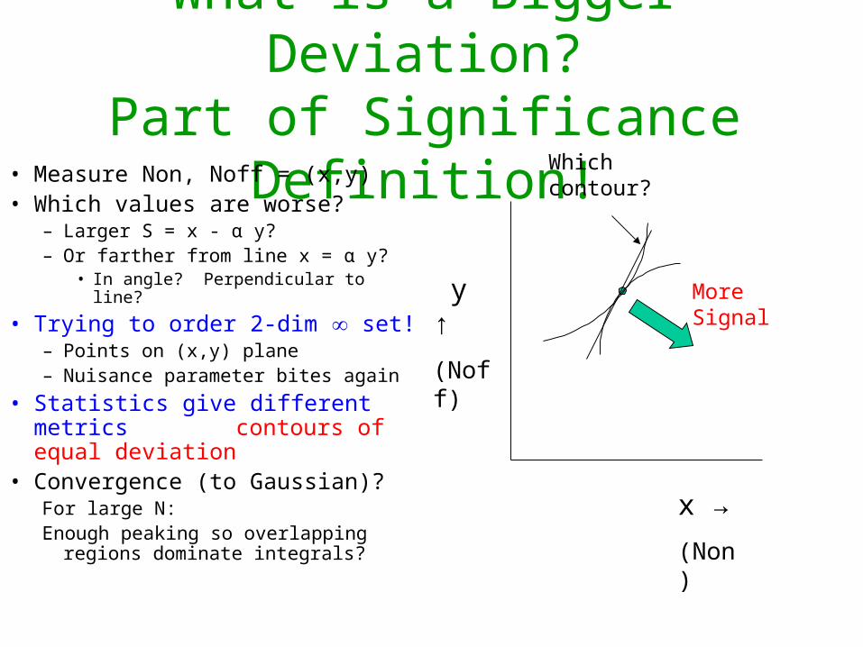
What is a Bigger Deviation?Part of Significance Definition!
• Measure Non, Noff = (x,y)• Which values are worse?
– Larger S = x - α y?– Or farther from line x = α y?
• In angle? Perpendicular to line?
• Trying to order 2-dim set!– Points on (x,y) plane– Nuisance parameter bites again
• Statistics give different metrics contours of equal deviation
• Convergence (to Gaussian)? For large N:Enough peaking so overlapping regions
dominate integrals?
y ↑
(Noff)
x →
(Non)
More Signal
Which contour?
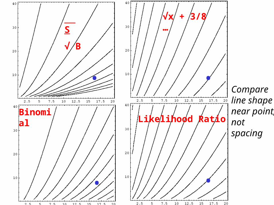
S
√ B
9
Likelihood RatioBinomial
√x + 3/8 …
Compare line shape near point, not spacing
• •
••
To Do
• Monte Carlo Tests
• Fraser-Reid for full problem• Nuisance parameter treatment, geometry
• Canonical parameter?
– Simpler numerics, if it works!• But: problems for large Z ?
• And for large N?
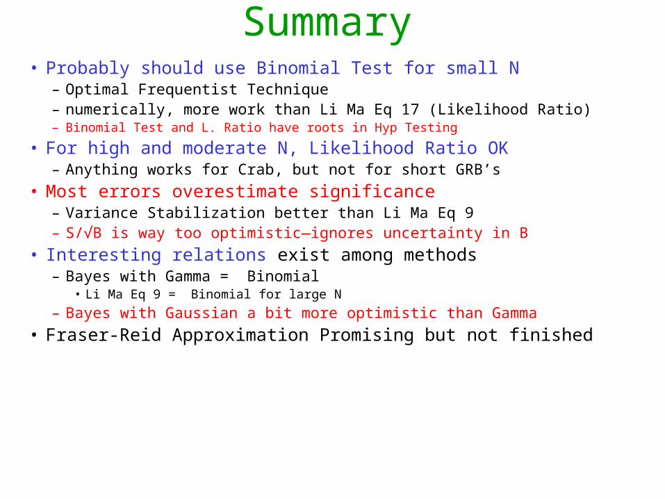
Summary• Probably should use Binomial Test for small N
– Optimal Frequentist Technique– numerically, more work than Li Ma Eq 17 (Likelihood Ratio)– Binomial Test and L. Ratio have roots in Hyp Testing
• For high and moderate N, Likelihood Ratio OK – Anything works for Crab, but not for short GRB’s
• Most errors overestimate significance– Variance Stabilization better than Li Ma Eq 9– S/√B is way too optimistic—ignores uncertainty in B
• Interesting relations exist among methods– Bayes with Gamma = Binomial
• Li Ma Eq 9 = Binomial for large N
– Bayes with Gaussian a bit more optimistic than Gamma
• Fraser-Reid Approximation Promising but not finished
References
Li & Ma Astroph. Journ. 272 (1983) 314-324Zhang & Ramsden Experimental Astronomy 1 (1990)
145-163Fraser Journ. Am. Stat. Soc. 86 (1990) 258-265Alexandreas et. al. Nuc. Inst. & Meth. A328 (1993) 570-
577
Gelman et. al., Bayesian Data Analysis, Chapman & Hall (1998)(predictive p-value terminology)
Talks: http://www-conf.slac.stanford.edu/phystat2003/
Controlling theFalse Discovery Rate: From Astrophysics to
Bioinformatics
The Problem:• I: You have a really good idea. You find a
positive effect at the .05 significance level.
• II: While you are in Stockholm, your students work very hard. They follow up on 100 of your ideas, but have somehow misinterpreted your brilliant notes. Still, they report 5 of them gave significant results. Do you book a return flight?
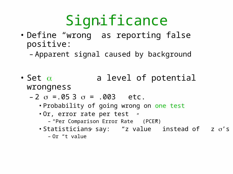
Significance• Define “wrong” as reporting false positive:
– Apparent signal caused by background
• Set a level of potential wrongness– 2 =.05 3 = .003 etc.
• Probability of going wrong on one test• Or, error rate per test
– “Per Comparison Error Rate” (PCER)
• Statisticians say: “z value” instead of z ’s– Or “t value”
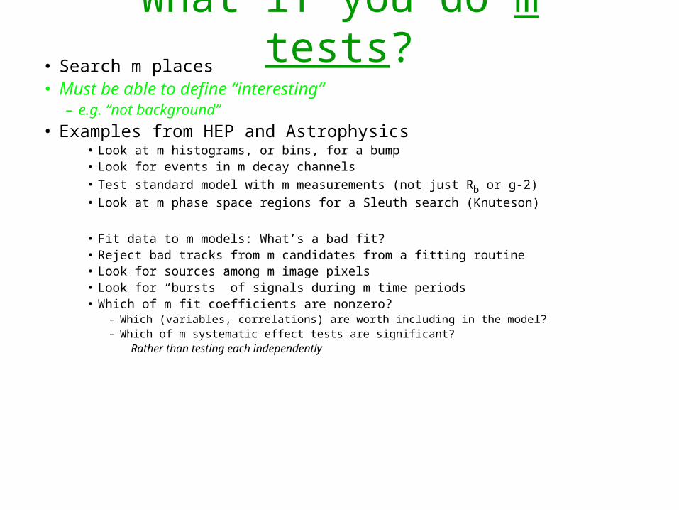
What if you do m tests?• Search m places• Must be able to define “interesting”
– e.g. “not background”
• Examples from HEP and Astrophysics• Look at m histograms, or bins, for a bump• Look for events in m decay channels
• Test standard model with m measurements (not just Rb or g-2)
• Look at m phase space regions for a Sleuth search (Knuteson)
• Fit data to m models: What’s a bad fit?• Reject bad tracks from m candidates from a fitting routine• Look for sources among m image pixels• Look for “bursts” of signals during m time periods• Which of m fit coefficients are nonzero?
– Which (variables, correlations) are worth including in the model?– Which of m systematic effect tests are significant?
Rather than testing each independently
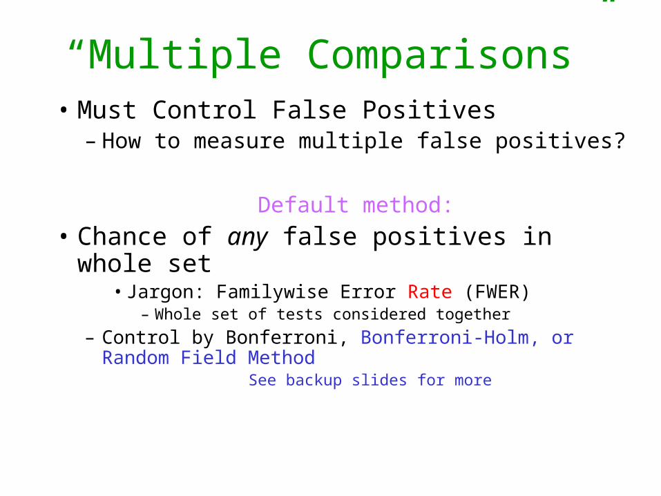
“Multiple Comparisons”• Must Control False Positives
– How to measure multiple false positives?
Default method:
• Chance of any false positives in whole set• Jargon: Familywise Error Rate (FWER)
– Whole set of tests considered together
– Control by Bonferroni, Bonferroni-Holm, or Random Field Method
See backup slides for more
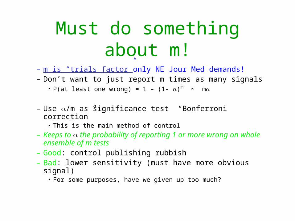
Must do something about m!
– m is “trials factor” only NE Jour Med demands!– Don’t want to just report m times as many signals
• P(at least one wrong) = 1 – (1- )m ~ m
– Use /m as significance test “Bonferroni correction”• This is the main method of control
– Keeps to the probability of reporting 1 or more wrong on whole ensemble of m tests
– Good: control publishing rubbish– Bad: lower sensitivity (must have more obvious signal)
• For some purposes, have we given up too much?
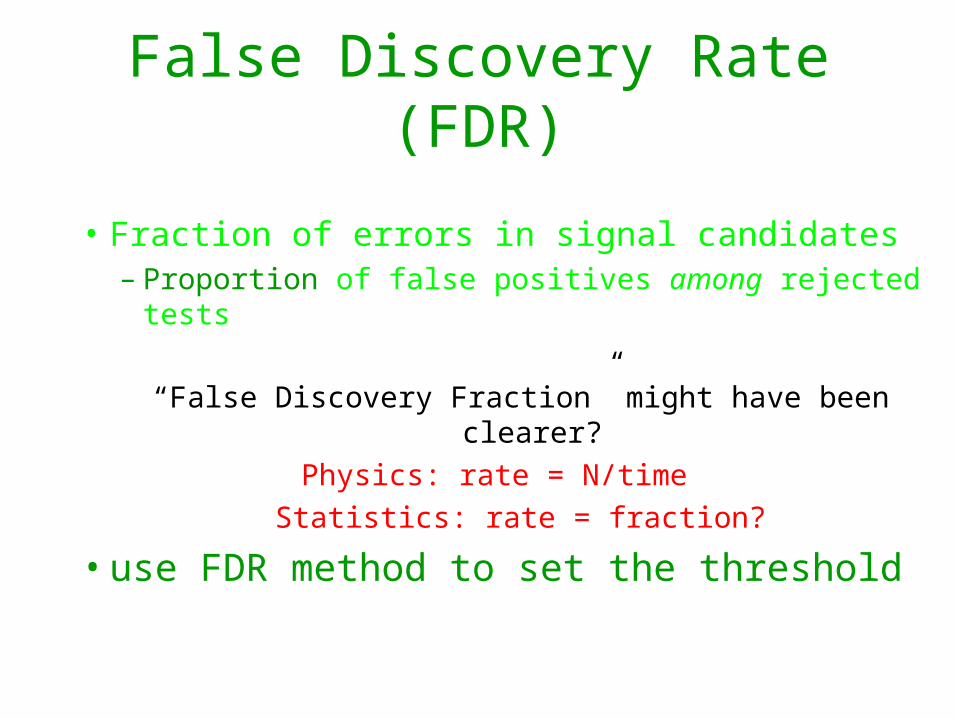
False Discovery Rate (FDR)
• Fraction of errors in signal candidates– Proportion of false positives among rejected tests
“False Discovery Fraction” might have been clearer?
Physics: rate = N/time Statistics: rate = fraction?
• use FDR method to set the threshold
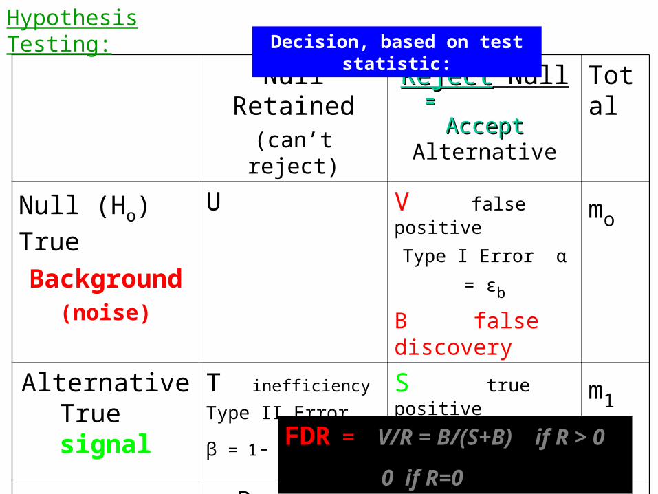
Null Retained(can’t reject)
RejectReject Null ==
AcceptAccept AlternativeTotal
Null (Ho) True
Background(noise)
U V false positive
Type I Error α = εb
B false discovery
mo
Alternative True signal
T inefficiency
Type II Error β = 1- εs
S true positive
true detectionm1
m-R R reported signal
= S+B rejections
m
FDR = V/R = B/(S+B) if R > 0
0 if R=0
Decision, based on test statistic:Hypothesis Testing:
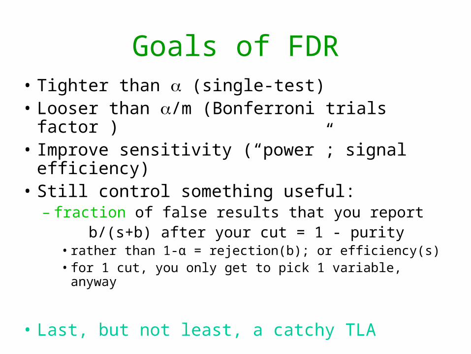
Goals of FDR• Tighter than (single-test)• Looser than /m (Bonferroni trials factor )• Improve sensitivity (“power”; signal efficiency)• Still control something useful:
– fraction of false results that you reportb/(s+b) after your cut = 1 - purity
• rather than 1-α = rejection(b); or efficiency(s)• for 1 cut, you only get to pick 1 variable, anyway
• Last, but not least, a catchy TLA
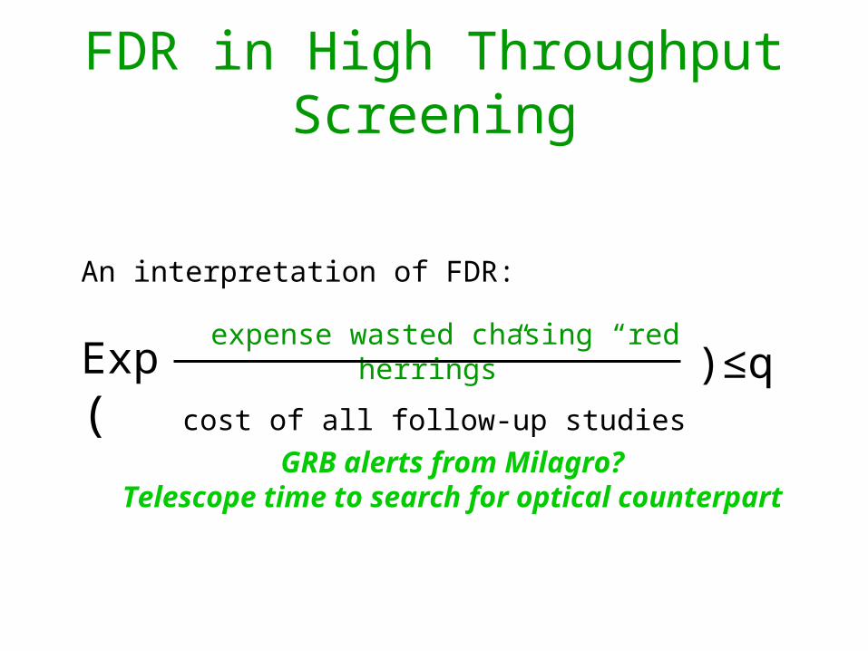
FDR in High Throughput Screening
An interpretation of FDR:
expense wasted chasing “red herrings”
cost of all follow-up studies Exp( )≤q
GRB alerts from Milagro?Telescope time to search for optical counterpart
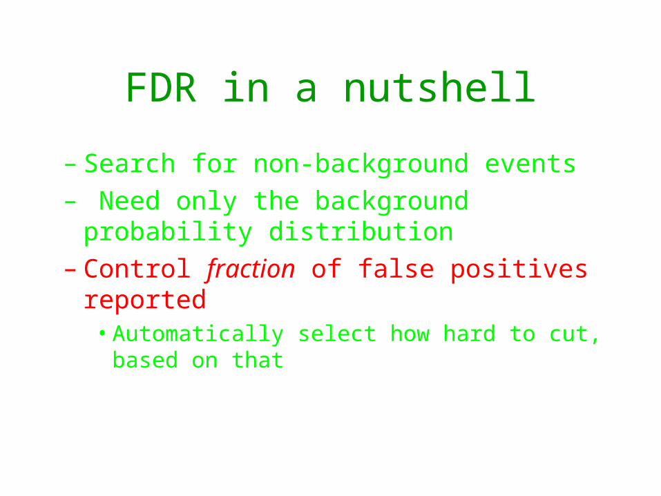
FDR in a nutshell
– Search for non-background events– Need only the background probability distribution– Control fraction of false positives reported
• Automatically select how hard to cut, based on that
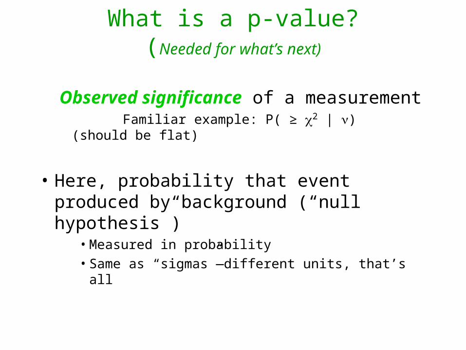
What is a p-value?(Needed for what’s next)
Observed significance of a measurement Familiar example: P( ≥ 2 | ) (should be flat)
• Here, probability that event produced by background (“null hypothesis”)
• Measured in probability
• Same as “sigmas”—different units, that’s all
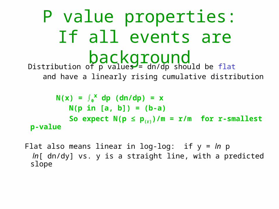
P value properties: If all events are background
Distribution of p values = dn/dp should be flat and have a linearly rising cumulative distribution
N(x) = ∫0x dp (dn/dp) = x
N(p in [a, b]) = (b-a)
So expect N(p ≤ p(r))/m = r/m for r-smallest p-value
Flat also means linear in log-log: if y = ln p ln[ dn/dy] vs. y is a straight line, with a predicted slope
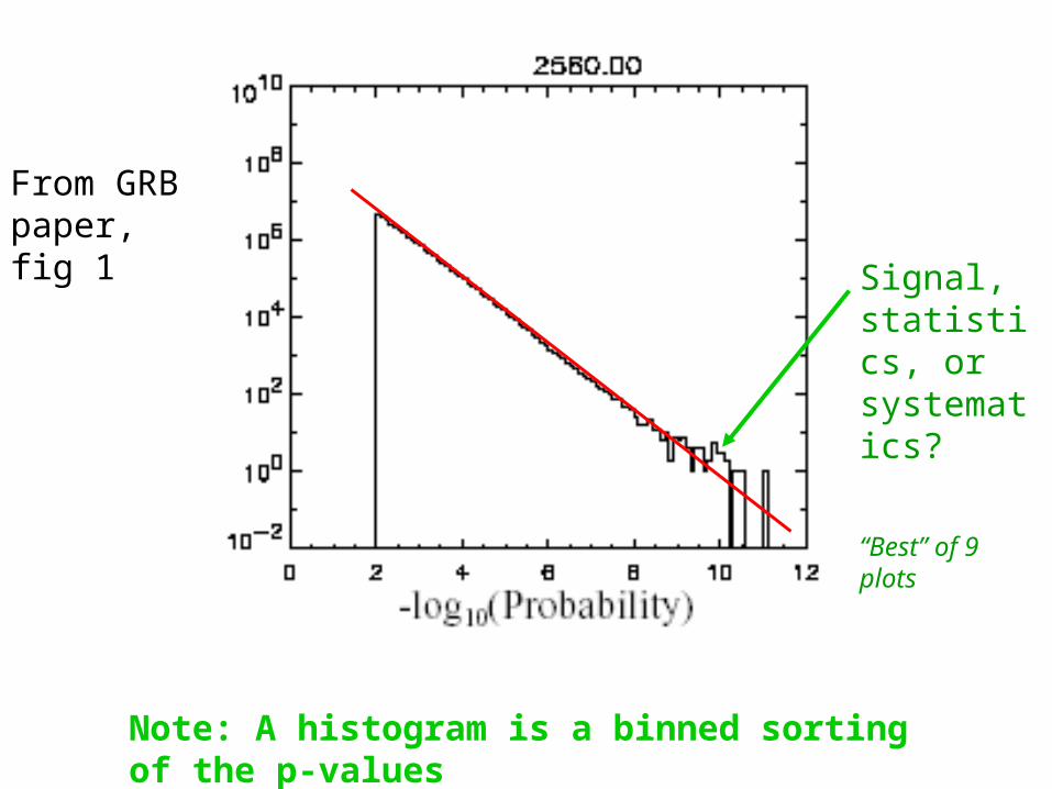
Note: A histogram is a binned sorting of the p-values
From GRB paper, fig 1
Signal, statistics, or systematics?
“Best” of 9 plots
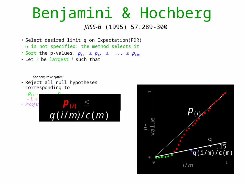
Benjamini & Hochberg
• Select desired limit q on Expectation(FDR) is not specified: the method selects it
• Sort the p-values, p(1) p(2) ... p(m)
• Let r be largest i such that
For now, take c(m)=1
• Reject all null hypotheses corresponding to p(1), ... , p(r).– i.e. Accept as signalAccept as signal
• Proof this works is not obvious!p(i) q(i/m)/c(m)
p(i)
i/m
q(i/m)/c(m)p-
valu
e
0 1
01
JRSS-B (1995) 57:289-300
q ~ .15
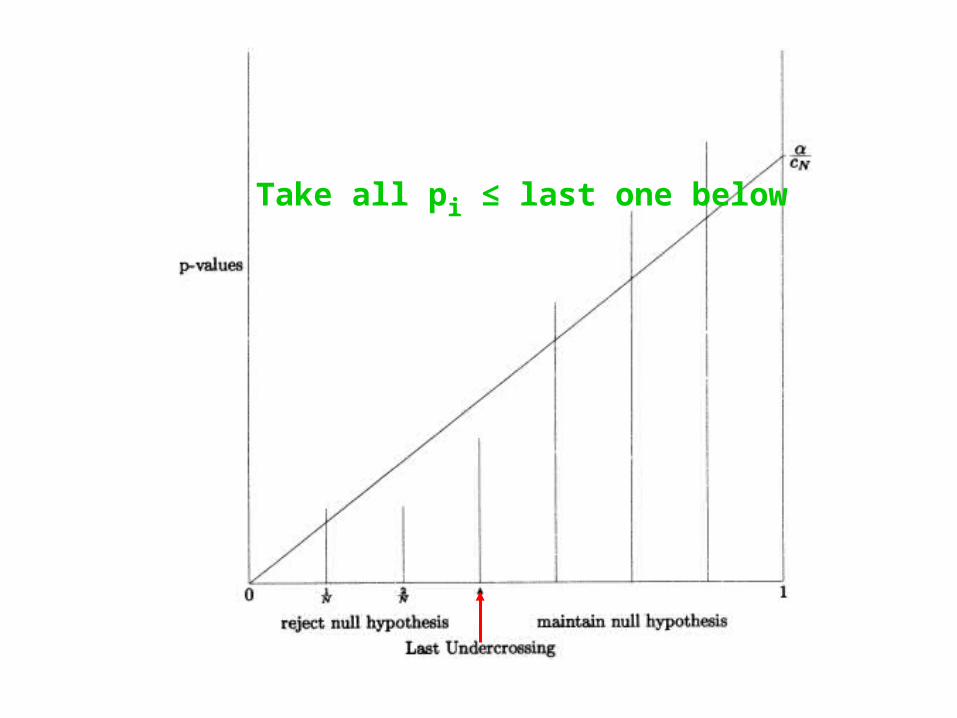
Take all pi ≤ last one below
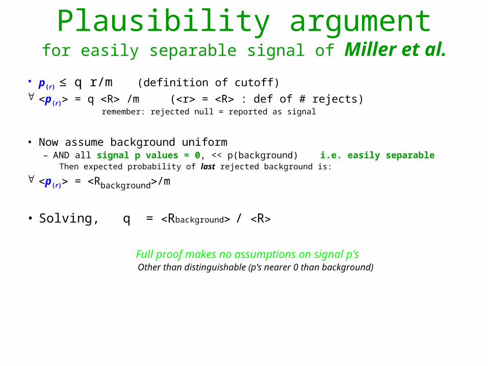
Plausibility argumentfor easily separable signal of Miller et al.
• p(r) ≤ q r/m (definition of cutoff) p(r) = q R /m (r = R : def of # rejects)
remember: rejected null = reported as signal
• Now assume background uniform– AND all signal p values ≈ 0, << p(background) i.e. easily separable
Then expected probability of last rejected background is:
p(r) = Rbackground/m
• Solving, q = Rbackground / R
Full proof makes no assumptions on signal p’sOther than distinguishable (p’s nearer 0 than background)
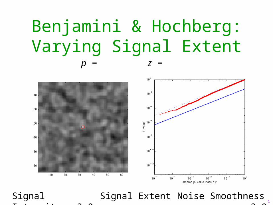
Benjamini & Hochberg:Varying Signal Extent
Signal Intensity 3.0 Signal Extent 1.0 Noise Smoothness 3.0
p = z =
1
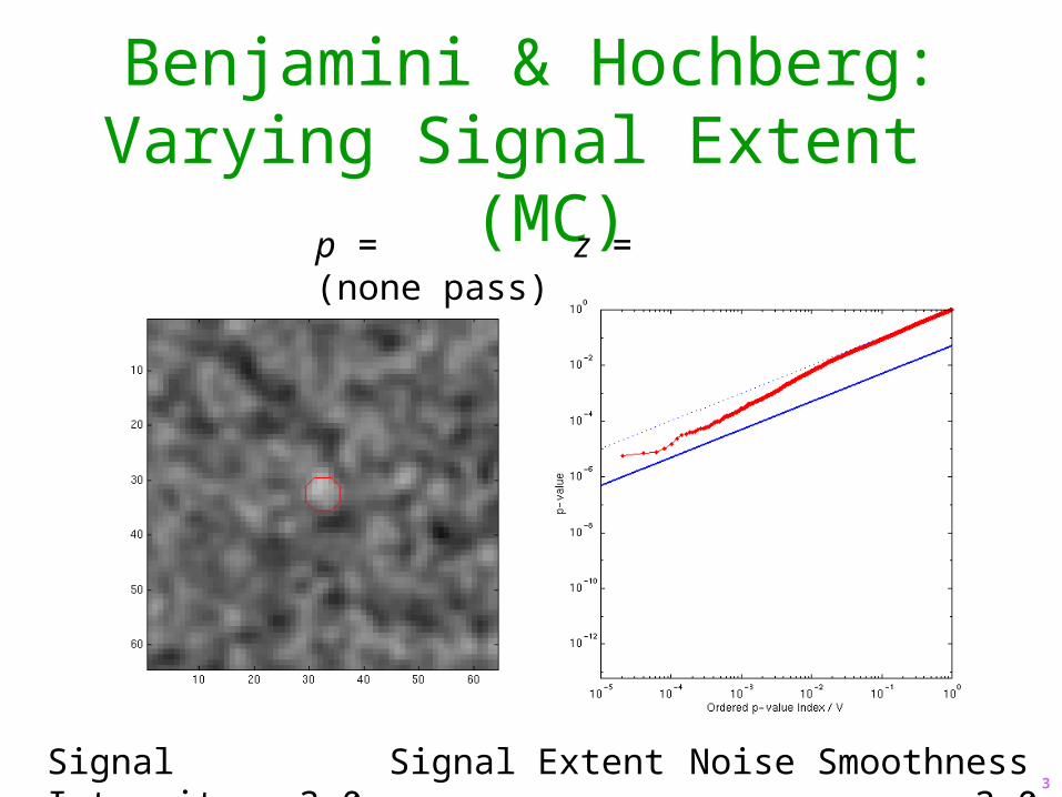
Benjamini & Hochberg:Varying Signal Extent (MC)
Signal Intensity 3.0 Signal Extent 3.0 Noise Smoothness 3.0
p = z = (none pass)
3
Flat
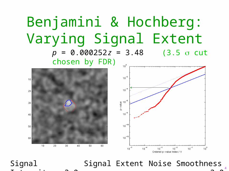
Benjamini & Hochberg:Varying Signal Extent
Signal Intensity 3.0 Signal Extent 5.0 Noise Smoothness 3.0
p = 0.000252 z = 3.48 (3.5 cut chosen by FDR)
4
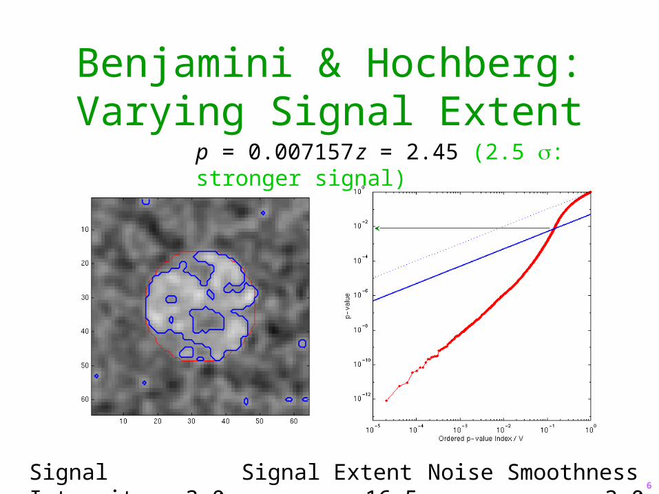
Benjamini & Hochberg:Varying Signal Extent
Signal Intensity 3.0 Signal Extent 16.5 Noise Smoothness 3.0
p = 0.007157 z = 2.45 (2.5 : stronger signal)
6
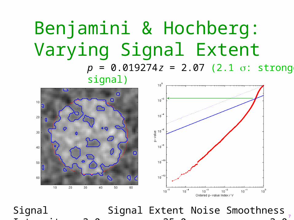
Benjamini & Hochberg:Varying Signal Extent
Signal Intensity 3.0 Signal Extent 25.0 Noise Smoothness 3.0
p = 0.019274 z = 2.07 (2.1 : stronger signal)
7
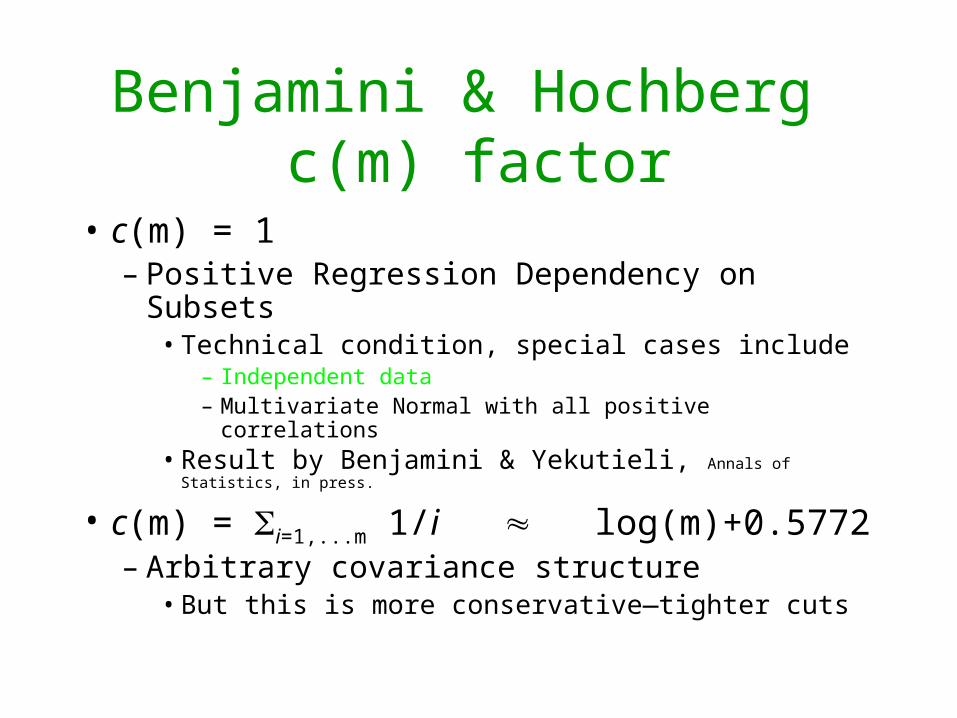
Benjamini & Hochberg c(m) factor
• c(m) = 1– Positive Regression Dependency on Subsets
• Technical condition, special cases include– Independent data– Multivariate Normal with all positive correlations
• Result by Benjamini & Yekutieli, Annals of Statistics, in press.
• c(m) = i=1,...m 1/i log(m)+0.5772– Arbitrary covariance structure
• But this is more conservative—tighter cuts
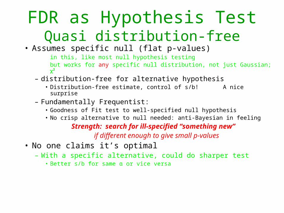
FDR as Hypothesis TestQuasi distribution-free
• Assumes specific null (flat p-values) in this, like most null hypothesis testingbut works for any specific null distribution, not just Gaussian; 2
– distribution-free for alternative hypothesis• Distribution-free estimate, control of s/b! A nice surprise
– Fundamentally Frequentist: • Goodness of Fit test to well-specified null hypothesis• No crisp alternative to null needed: anti-Bayesian in feeling
Strength: search for ill-specified “something new”if different enough to give small p-values
• No one claims it’s optimal– With a specific alternative, could do sharper test
• Better s/b for same α or vice versa
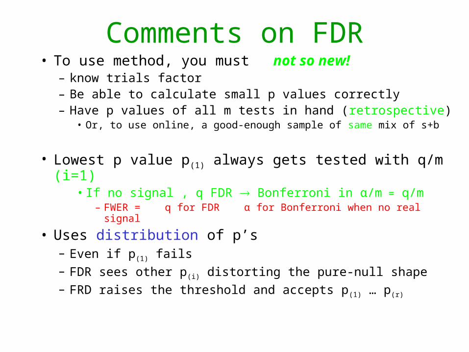
Comments on FDR• To use method, you must not so new!
– know trials factor– Be able to calculate small p values correctly– Have p values of all m tests in hand (retrospective)
• Or, to use online, a good-enough sample of same mix of s+b
• Lowest p value p(1) always gets tested with q/m (i=1)• If no signal , q FDR Bonferroni in α/m = q/m
– FWER = q for FDR α for Bonferroni when no real signal
• Uses distribution of p’s– Even if p(1) fails– FDR sees other p(i) distorting the pure-null shape – FRD raises the threshold and accepts p(1) … p(r)
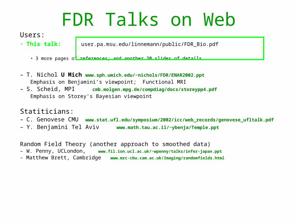
FDR Talks on WebUsers:– This talk: user.pa.msu.edu/linnemann/public/FDR_Bio.pdf
• 3 more pages of references; and another 30 slides of details
– T. Nichol U Mich www.sph.umich.edu/~nichols/FDR/ENAR2002.ppt Emphasis on Benjamini’s viewpoint; Functional MRI
– S. Scheid, MPI cmb.molgen.mpg.de/compdiag/docs/storeypp4.pdf
Emphasis on Storey’s Bayesian viewpoint
Statiticians:– C. Genovese CMU www.stat.ufl.edu/symposium/2002/icc/web_records/genovese_ufltalk.pdf
– Y. Benjamini Tel Aviv www.math.tau.ac.il/~ybenja/Temple.ppt
Random Field Theory (another approach to smoothed data)– W. Penny, UCLondon, www.fil.ion.ucl.ac.uk/~wpenny/talks/infer-japan.ppt
- Matthew Brett, Cambridge www.mrc-cbu.cam.ac.uk/Imaging/randomfields.html
Some other web pages
• http://medir.ohsu.edu/~geneview/education/Multiple test corrections.pdf
Brief summary of the main methods
• www.unt.edu/benchmarks/archives/2002/april02/rss.htm
Gentle introduction to FDR
www.sph.umich.edu/~nichols/FDR/FDR resources and references—imaging
http://www.math.tau.ac.il/~roee/index.htmFDR resource page by discoverer
Some FDR Papers on WebAstrophysicsarxiv.org/abs/astro-ph/0107034 Miller et. al. ApJ 122: 3492-3505 Dec 2001
FDR explained very clearly; heuristic proof for well-separated signal
arxiv.org/abs/astro-ph/0110570 Hopkins et. Al. ApJ 123: 1086-1094 Dec 2002
2d pixel images; compare FDR to other methodstaos.asiaa.sinica.edu.tw/document/chyng_taos_paper.pdf FDR comet search (by occultations)
will set tiny FDR limit 10-12 ~ 1/year
Statisticshttp://www.math.tau.ac.il/~ybenja/depApr27.pdf Benjamini et al: (invented FDR)
clarifies c(m) for different dependences of data
Benjamani, Hochberg: JRoyalStatSoc-B (1995) 57:289-300 paper not on the web defined FDR, and Bonferroni-Holm procedure
http://www-stat.stanford.edu/~donoho/Reports/2000/AUSCFDR.pdf Benjamani et alstudy small signal fraction (sparsity), relate to minimax loss
http://www.stat.cmu.edu/www/cmu-stats/tr/tr762/tr762.pdf Genovese, Wasserman conf limits for FDR; study for large m; another view of FDR as data-estimated method on mixtures
http://stat-www.berkeley.edu/~storey/ Storey view in terms of mixtures, Bayes; sharpen with data; some intuition for proof
http://www-stat.stanford.edu/~tibs/research.html Efron, Storey, Tibshirani show Empirical Bayes equivalent to BH FDR