measurement systems analysis manual is an introduction to measurement system analysis. it is not...
TRANSCRIPT

i
MEASUREMENT SYSTEMS ANALYSIS
Reference Manual Fourth Edition
First Edition, October 1990 • Second Edition, February 1995; Second Printing, June 1998 Third Edition, March 2002; Second Printing, May 2003; Fourth Edition, June 2010
Copyright © 1990, © 1995, © 2002, © 2010 Chrysler Group LLC, Ford Motor Company, General Motors Corporation ISBN#: 978-1-60-534211-5

ii

iii
FOREWORD
This Reference Manual was developed by a Measurement Systems Analysis (MSA) Work Group, sanctioned by the Chrysler Group LLC, Ford Motor Company, and General Motors Corporation Supplier Quality Requirements Task Force, and under the auspices of the Automotive Industry Action Group (AIAG). The Work Group responsible for this Fourth Edition were Michael Down (General Motors Corporation), Frederick Czubak (Chrysler Group LLC), Gregory Gruska (Omnex), Steve Stahley (Cummins, Inc.) and David Benham. The manual is an introduction to measurement system analysis. It is not intended to limit evolution of analysis methods suited to particular processes or commodities. While these guidelines are intended to cover normally occurring measurement system situations, there will be questions that arise. These questions should be directed to your authorized customer representative. This Manual is copyrighted by Chrysler Group LLC, Ford Motor Company, and General Motors Corporation, with all rights reserved, 2010. Additional manuals can be ordered from AIAG at Uwww.aiag.org T. Permission to reproduce portions of this manual for use within supplier organizations may be obtained from AIAG at Uwww.aiag.org T
June 2010

iv
MSA 4th Edition Quick Guide
Type of
Measurement System MSA Methods Chapter
Basic Variable Range, Average & Range, ANOVA,
Bias, Linearity, Control Charts III
Basic Attribute Signal Detection,
Hypothesis Test Analyses III
Non-Replicable (e.g., Destructive Tests)
Alternate Approaches IV
Complex Variable Range, Average & Range, ANOVA,
Bias Linearity Control Charts III, IV
Multiple Systems, Gages or Test Stands
Control Charts ANOVA Regression Analysis III, IV
Miscellaneous Alternate Approaches IV
Other White Papers – available at
AIAG website (www.aiag.org)
NOTE: Regarding the use of the GRR standard deviation Historically, by convention, a 99% spread has been used to represent the “full” spread of measurement error, represented by a 5.15 multiplying factor (where GRR is multiplied by 5.15
to represent a total spread of 99%). A 99.73% spread is represented by a multiplier of 6.0, which is 3 and represents the full spread of a “normal” curve. If the reader chooses to increase the coverage level, or spread, of the total measurement variation to 99.73%, use 6.0 as a multiplier in place of 5.15 in the calculations. Note: The approach used in the 4th Edition is to compare standard deviations. This is equivalent to using the multiplier of 6 in the historical approach. Awareness of which multiplying factor is used is crucial to the integrity of the equations and resultant calculations. This is especially important if a comparison is to be made between measurement system variability and the tolerance. Consequently, if an approach other than that described in this manual is used, a statement of such must be stated clearly in any results or summaries (particularly those provided to the customer).

v
TABLE OF CONTENTS
MSA 4th Edition Quick Guide .....................................................................................................................................iv TABLE OF CONTENTS ............................................................................................................................................v List of Tables............................................................................................................................................................. vii List of Figures .......................................................................................................................................................... viii CHAPTER I General Measurement System Guidelines.........................................................................................1
Section A Introduction, Purpose and Terminology ...................................................................................................3 Introduction ...........................................................................................................................................................3 Purpose ..................................................................................................................................................................4 Terminology ..........................................................................................................................................................4
Section B The Measurement Process P.....................................................................................................................13 Measurement Systems .........................................................................................................................................13 The Effects of Measurement System Variability.................................................................................................18
Section C Measurement Strategy and Planning.......................................................................................................25 Section D Measurement Source Development .......................................................................................................29
Gage Source Selection Process............................................................................................................................31 Section E Measurement Issues ................................................................................................................................41 Section F Measurement Uncertainty........................................................................................................................63 Section G Measurement Problem Analysis .............................................................................................................65
CHAPTER II General Concepts for Assessing Measurement Systems ...............................................................67 Section A Background.............................................................................................................................................69 Section B Selecting/Developing Test Procedures....................................................................................................71 Section C Preparation for a Measurement System Study ........................................................................................73 Section D Analysis of the Results............................................................................................................................77
CHAPTER III Recommended Practices for Replicable Measurement Systems ................................................81 Section A Example Test Procedures........................................................................................................................83 Section B Variable Measurement System Study Guidelines ...................................................................................85
Guidelines for Determining Stability...................................................................................................................85 Guidelines for Determining Bias PF – Independent Sample Method ...................................................................87 Guidelines for Determining Bias – Control Chart Method..................................................................................92 Guidelines for Determining Linearity P................................................................................................................96 Guidelines for Determining Repeatability and Reproducibility P ......................................................................101 Range Method....................................................................................................................................................102 Average and Range Method ..............................................................................................................................103 Analysis of Variance (ANOVA) Method ..........................................................................................................123
Section C Attribute Measurement Systems Study .................................................................................................131 Risk Analysis Methods ......................................................................................................................................131 Signal Detection Approach................................................................................................................................143 Analytic Method P ..............................................................................................................................................145
CHAPTER IV Other Measurement Concepts and Practices .............................................................................151 Section A Practices for Non-Replicable Measurement Systems ...........................................................................153
Destructive measurement systems .....................................................................................................................153 Systems where the part changes on use/test ......................................................................................................153
Section B Stability Studies ....................................................................................................................................155 Section C Variability Studies.................................................................................................................................161 Section D Recognizing the Effect of Excessive Within-Part Variation................................................................167 Section E Average and Range Method – Additional Treatment............................................................................169 Section F Gage Performance Curve P.....................................................................................................................177 Section G Reducing Variation Through Multiple Readings ..................................................................................183 Section H Pooled Standard Deviation Approach to GRR P ....................................................................................185
APPENDICES..........................................................................................................................................................193
vi
Appendix A...............................................................................................................................................................195 Analysis of Variance Concepts..............................................................................................................................195
Appendix B...............................................................................................................................................................199 Impact of GRR on the Capability Index Cp ...........................................................................................................199 Formulas:...............................................................................................................................................................199 Analysis: ................................................................................................................................................................199 Graphical Analysis ................................................................................................................................................201
Appendix C...............................................................................................................................................................203 Appendix D...............................................................................................................................................................205
Gage R Study.........................................................................................................................................................205 Appendix E...............................................................................................................................................................207
Alternate PV Calculation Using Error Correction Term........................................................................................207 Appendix F ...............................................................................................................................................................209
P.I.S.M.O.E.A. Error Model..................................................................................................................................209 Glossary....................................................................................................................................................................213 Reference List ..........................................................................................................................................................219 Sample Forms ..........................................................................................................................................................223 Index .........................................................................................................................................................................227

vii
List of Tables Table I-B1: Control Philosophy and Driving Interest..................................................................................18 Table II-D 1: GRR Criteria...........................................................................................................................78 Table III-B 1: Bias Study Data....................................................................................................................90 Table III-B 2: Bias Study – Analysis of Bias Study P..................................................................................92 Table III-B 3: Bias Study – Analysis of Stability Study for Bias..................................................................95 Table III-B 4: Linearity Study Data .............................................................................................................99 Table III-B 5: Linearity Study – Intermediate Results ................................................................................99 Table III-B 6: Gage Study (Range Method) .............................................................................................103 Table III-B 6a: Gage Repeatability and Reproducibility Data Collection Sheet .......................................105 Table III-B 7: ANOVA Table .....................................................................................................................127 Table III-B 8: ANOVA Analysis % Variation & Contribution ......................................................................127 Table III-B 9: Comparison of ANOVA and Average and Range Methods ...............................................129 Table III-B 10: GRR ANOVA Method Report ..........................................................................................129 Table III-C 1: Attribute Study Data Set......................................................................................................134 Table III-C 2: Cross tabulation Study Results ...........................................................................................136 Table III-C 3: Kappa Summary .................................................................................................................137 Table III-C 4: Comparisons of Appraisers to Reference ...........................................................................138 Table III-C 5: Study Effectiveness Table...................................................................................................139 Table III-C 6: Example Effectiveness Criteria Guidelines .........................................................................140 Table III-C 7: Study Effectiveness Summary ............................................................................................140 Table III-C 8: Table III-C 1 sorted by Ref Value........................................................................................143 Table IV-A 1: Methods Based on Type of Measurement System............................................................154 Table IV-H 1: Pooled Standard Deviation Analysis Data Set ...................................................................189 Table A 1: Estimate of Variance Components .........................................................................................195 Table A 2: 6 Sigma Spread......................................................................................................................196 Table A 3: Analysis of Variance (ANOVA) ...............................................................................................197 Table A 4: Tabulated ANOVA Results .....................................................................................................198 Table A 5: Tabulated ANOVA Results .....................................................................................................198 Table B 1: Comparison of Observed to Actual Cp ...................................................................................201
Table C 1: *2d Table ..............................................................................................................................203
Table F 1: Examples of the PISMOEA Model..........................................................................................211

viii
List of Figures UFigure I-A 1: Example of a Traceability Chain for a Length MeasurementT ................................................10 UFigure I-B 1: Measurement System Variability Cause and Effect DiagramT ................................................17 UFigure I-E 2: DiscriminationT........................................................................................................................46 UFigure I-E 3: Impact of Number of Distinct Categories (ndc) of the Process Distribution on Control and
Analysis Activities T ................................................................................................................................47 UFigure I-E 4: Process Control ChartsT .........................................................................................................49 UFigure I-E 5: Characteristics of the Measurement Process VariationT .........................................................50 UFigure I-E 6: Relationships between Bias and Repeatability T .....................................................................62 UFigure III-B 1: Control Chart Analysis for Stability T .....................................................................................86 UFigure III-B 2: Bias Study – Histogram of Bias StudyT ................................................................................91 UFigure III-B 3: Linearity Study – Graphical Analysis T ................................................................................100 UFigure III-B 4: Average Chart – “Stacked” T................................................................................................107 UFigure III-B 5: Average Chart – “Unstacked”T............................................................................................107 UFigure III-B 6: Range Chart – “Stacked” T ..................................................................................................108 UFigure III-B 7: Range Chart – “Unstacked”T ..............................................................................................109 UFigure III-B 8: Run Chart by Part T .............................................................................................................109 UFigure III-B 9: Scatter PlotT........................................................................................................................110 UFigure III-B 10: Whiskers Chart T................................................................................................................111 UFigure III-B 11: Error Charts T.....................................................................................................................112 UFigure III-B 12: Normalized Histogram T.....................................................................................................113 UFigure III-B 13: X–Y Plot of Averages by Size T .........................................................................................114 UFigure III-B 14: Comparison X–Y Plots T ....................................................................................................115 UFigure III-B 15: Completed GR&R Data Collection SheetT .......................................................................118 UFigure III-B 16: Gage Repeatability and Reproducibility Report T ..............................................................119 UFigure III-B 18: Residual Plot T ...................................................................................................................126 UFigure III-C 1: Example Process with Pp = Ppk = 0.50T.............................................................................132 UFigure III-C 2: The “Gray” Areas Associated with the Measurement SystemT ...........................................132 UFigure III-C 3: Example Process with Pp = Ppk = 1.33T.............................................................................141 UFigure III-C 4: Attribute Gage Performance Curve Plotted on Normal Probability PaperT ........................149 UFigure III-C 5. Attribute Gage Performance CurveT ..................................................................................150 UFigure IV-E 1: Measurement Evaluation Control Chart ( T &X R U) - 1T......................................................172 UFigure IV-E 2: Measurement Evaluation Control Chart ( T &X R U) - 2T......................................................173 UFigure IV-E 3: Alternate Computations for Evaluating a Measurement Process (Part 1 of 2).T................174 UFigure IV-E 4: Alternate Computations for Evaluating a Measurement Process (Part 2 of 2).T................175 UFigure IV-F 1: Gage Performance Curve Without Error T...........................................................................180 UFigure IV-F 2: Gage Performance Curve –ExampleT ................................................................................181 UFigure IV-F 3: Gage Performance Curve Plotted on Normal Probability Paper T ......................................182 UFigure IV-H 1: Pooled Standard Deviation Study Graphical Analysis T .....................................................188 UFigure IV-H 2: Dot diagram of h values.T...................................................................................................191 UFigure IV-H 3: Dot diagram of k values.T ...................................................................................................192 UFigure B 1: Observed vs. Actual Cp (process based) T..............................................................................201 UFigure B 2: Observed vs. Actual Cp (tolerance based) T ...........................................................................202
Chapter I General Measurement System Guidelines
1
CHAPTER I
General Measurement System Guidelines

Chapter I – Section A Introduction, Purpose and Terminology
2
Chapter I – Section A Introduction, Purpose and Terminology
3
Quality of Measurement Data
Section A Introduction, Purpose and Terminology Introduction
Measurement data are used more often and in more ways than ever before. For instance, the decision to adjust a manufacturing process is now commonly based on measurement data. The data, or some statistic calculated from them, are compared with statistical control limits for the process, and if the comparison indicates that the process is out of statistical control, then an adjustment of some kind is made. Otherwise, the process is allowed to run without adjustment. Another use of measurement data is to determine if a significant relationship exists between two or more variables. For example, it may be suspected that a critical dimension on a molded plastic part is related to the temperature of the feed material. That possible relationship could be studied by using a statistical procedure called regression analysis to compare measurements of the critical dimension with measurements of the temperature of the feed material.
Studies that explore such relationships are examples of what Dr. W. E. Deming called analytic studies. In general, an analytic study is one that increases knowledge about the system of causes that affect the process. Analytic studies are among the most important uses of measurement data because they lead ultimately to better understanding of processes.
The benefit of using a data-based procedure is largely determined by the quality of the measurement data used. If the data quality is low, the benefit of the procedure is likely to be low. Similarly, if the quality of the data is high, the benefit is likely to be high also.
To ensure that the benefit derived from using measurement data is great enough to warrant the cost of obtaining it, attention needs to be focused on the quality of the data.
The quality of measurement data is defined by the statistical properties of multiple measurements obtained from a measurement system operating under stable conditions. For instance, suppose that a measurement system, operating under stable conditions, is used to obtain several measurements of a certain characteristic. If the measurements are all “close” to the master value for the characteristic, then the quality of the data is said to be “high”. Similarly, if some, or all, of the measurements are “far away” from the master value, then the quality of the data is said to be “low”.
The statistical properties most commonly used to characterize the quality of data are the bias and variance of the measurement system. The property called bias refers to the location of the data relative to a reference (master) value, and the property called variance refers to the spread of the data.
One of the most common reasons for low-quality data is too much variation. Much of the variation in a set of measurements may be due to the interaction between the measurement system and its environment. For instance, a
Chapter I – Section A Introduction, Purpose and Terminology
4
measurement system used to measure the volume of liquid in a tank may be sensitive to the ambient temperature of the environment in which it is used. In that case, variation in the data may be due either to changes in the volume or to changes in the ambient temperature. That makes interpreting the data more difficult and the measurement system, therefore, less desirable.
If the interaction generates too much variation, then the quality of the data may be so low that the data are not useful. For example, a measurement system with a large amount of variation may not be appropriate for use in analyzing a manufacturing process because the measurement system’s variation may mask the variation in the manufacturing process. Much of the work of managing a measurement system is directed at monitoring and controlling variation. Among other things, this means that emphasis needs to be placed on learning how the measurement system interacts with its environment so that only data of acceptable quality are generated.
Purpose
The purpose of this document is to present guidelines for assessing the quality of a measurement system. Although the guidelines are general enough to be used for any measurement system, they are intended primarily for the measurement systems used in the industrial world. This document is not intended to be a compendium of analyses for all measurement systems. Its primary focus is measurement systems where the readings can be replicated on each part. Many of the analyses are useful with other types of measurement systems and the manual does contain references and suggestions. It is recommended that competent statistical resources be consulted for more complex or unusual situations not discussed here. Customer approval is required for measurement systems analysis methods not covered in this manual.
Terminology
The discussion of the analysis of measurement system can become confusing and misleading without an established set of terms to refer to the common statistical properties and related elements of the measurement system. This section provides a summary of such terms which are used in this manual. In this document, the following terms are used:
Measurement is defined as “the assignment of numbers [or values] to material things to represent the relations among them with respect to particular properties.” This definition was first given by C. Eisenhart (1963). The process of assigning the numbers is defined as the measurement process, and the value assigned is defined as the measurement value.
Chapter I – Section A Introduction, Purpose and Terminology
5
Gage is any device used to obtain measurements; frequently used to refer specifically to the devices used on the shop floor; includes go/no-go devices (also, see Reference List: ASTM E456-96).
Measurement System is the collection of instruments or gages, standards, operations, methods, fixtures, software, personnel, environment and assumptions used to quantify a unit of measure or fix assessment to the feature characteristic being measured; the complete process used to obtain measurements.
From these definitions it follows that a measurement process may be viewed as a manufacturing process that produces numbers (data) for its output. Viewing a measurement system this way is useful because it allows us to bring to bear all the concepts, philosophy, and tools that have already demonstrated their usefulness in the area of statistical process control.
Summary of Terms P
1
Standard
Accepted basis for comparison
Criteria for acceptance
Known value, within stated limits of uncertainty, accepted as a true value
Reference value
A standard should be an operational definition: a definition which will yield the same results when applied by the supplier or customer, with the same meaning yesterday, today, and tomorrow.
Basic equipment
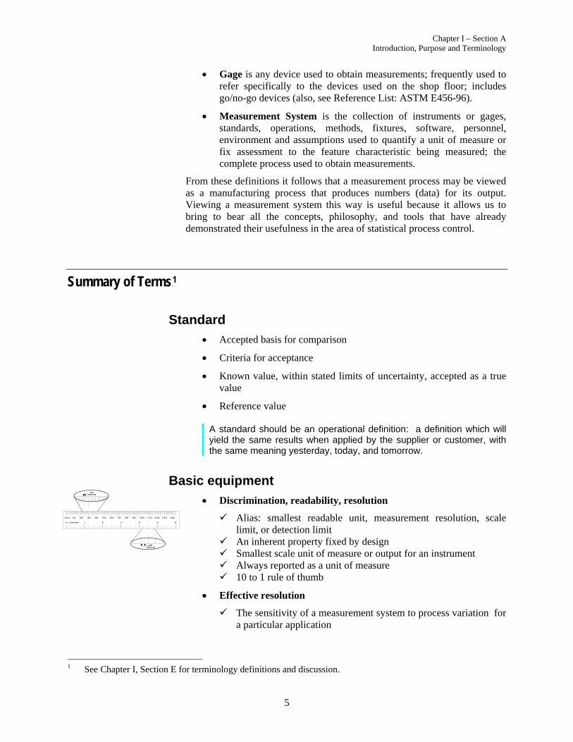
Discrimination, readability, resolution
Alias: smallest readable unit, measurement resolution, scale limit, or detection limit
An inherent property fixed by design Smallest scale unit of measure or output for an instrument Always reported as a unit of measure 10 to 1 rule of thumb
Effective resolution
The sensitivity of a measurement system to process variation for a particular application
1 See Chapter I, Section E for terminology definitions and discussion.

Chapter I – Section A Introduction, Purpose and Terminology
6
Smallest input that results in a usable output signal of measurement
Always reported as a unit of measure
Reference value
Accepted value of an artifact Requires an operational definition Used as the surrogate for the true value
True value
Actual value of an artifact Unknown and unknowable
Location variation
Accuracy
“Closeness” to the true value, or to an accepted reference value ASTM includes the effect of location and width errors
Bias
Difference between the observed average of measurements and the reference value
A systematic error component of the measurement system
Stability
The change in bias over time A stable measurement process is in statistical control with
respect to location Alias: Drift
Linearity
The change in bias over the normal operating range The correlation of multiple and independent bias errors over the
operating range A systematic error component of the measurement system
Chapter I – Section A Introduction, Purpose and Terminology
7
Width variation
Precision P
2
“Closeness” of repeated readings to each other A random error component of the measurement system
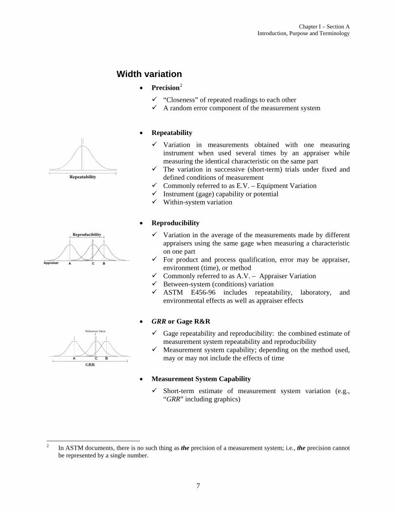
Repeatability
Variation in measurements obtained with one measuring instrument when used several times by an appraiser while measuring the identical characteristic on the same part
The variation in successive (short-term) trials under fixed and defined conditions of measurement
Commonly referred to as E.V. – Equipment Variation Instrument (gage) capability or potential Within-system variation
Reproducibility
Variation in the average of the measurements made by different appraisers using the same gage when measuring a characteristic on one part
For product and process qualification, error may be appraiser, environment (time), or method
Commonly referred to as A.V. – Appraiser Variation Between-system (conditions) variation ASTM E456-96 includes repeatability, laboratory, and
environmental effects as well as appraiser effects
GRR or Gage R&R
Gage repeatability and reproducibility: the combined estimate of measurement system repeatability and reproducibility
Measurement system capability; depending on the method used, may or may not include the effects of time
Measurement System Capability
Short-term estimate of measurement system variation (e.g., “GRR” including graphics)
2 In ASTM documents, there is no such thing as the precision of a measurement system; i.e., the precision cannot
be represented by a single number.
GRR
A C B
Reference Value
Chapter I – Section A Introduction, Purpose and Terminology
8
Measurement System Performance
Long-term estimate of measurement system variation (e.g., long-term Control Chart Method)
Sensitivity
Smallest input that results in a detectable output signal Responsiveness of the measurement system to changes in
measured feature Determined by gage design (discrimination), inherent quality
(Original Equipment Manufacturer), in-service maintenance, and operating condition of the instrument and standard
Always reported as a unit of measure
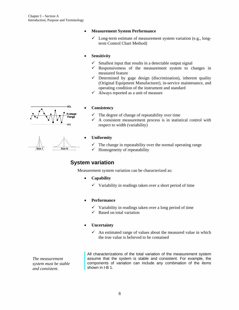
Consistency
The degree of change of repeatability over time A consistent measurement process is in statistical control with
respect to width (variability)
Uniformity
The change in repeatability over the normal operating range Homogeneity of repeatability
System variation Measurement system variation can be characterized as:
Capability
Variability in readings taken over a short period of time
Performance
Variability in readings taken over a long period of time Based on total variation
Uncertainty
An estimated range of values about the measured value in which the true value is believed to be contained
All characterizations of the total variation of the measurement system assume that the system is stable and consistent. For example, the components of variation can include any combination of the items shown in I-B 1.
The measurement system must be stable and consistent.

Chapter I – Section A Introduction, Purpose and Terminology
9
National Measurement Institutes
Traceability
Standards and Traceability
The National Institute of Standards and Technology (NIST) is the principal National Measurements Institute (NMI) in the United States serving under the U.S. Department of Commerce. NIST, formerly the National Bureau of Standards (NBS), serves as the highest level authority for metrology in the U.S. NIST’s primary responsibility is to provide measurement services and maintain measurement standards that assist U.S. industry in making traceable measurements which ultimately assist in trade of products and services. NIST provides these services directly to many types of industries, but primarily to those industries that require the highest level of accuracy for their products and that incorporate state-of-the-art measurements in their processes.
Most of the industrialized countries throughout the world maintain their own NMIs and similar to NIST, they also provide a high level of metrology standards or measurement services for their respective countries. NIST works collaboratively with these other NMIs to assure measurements made in one country do not differ from those made in another. This is accomplished through Mutual Recognition Arrangements (MRAs) and by performing interlaboratory comparisons between the NMIs. One thing to note is that the capabilities of these NMIs will vary from country to country and not all types of measurements are compared on a regular basis, so differences can exist. This is why it is important to understand to whom measurements are traceable and how traceable they are.
Traceability is an important concept in the trade of goods and services. Measurements that are traceable to the same or similar standards will agree more closely than those that are not traceable. This helps reduce the need for re-test, rejection of good product, and acceptance of bad product.
Traceability is defined by the ISO International Vocabulary of Basic and General Terms in Metrology (VIM) as:
“The property of a measurement or the value of a standard whereby it can be related to stated references, usually national or international standards, through an unbroken chain of comparisons all having stated uncertainties.”
The traceability of a measurement will typically be established through a chain of comparisons back to the NMI. However, in many instances in industry, the traceability of a measurement may be linked back to an agreed upon reference value or “consensus standard” between a customer and a supplier. The traceability linkage of these consensus standards to the NMI may not always be clearly understood, so ultimately it is critical that the measurements are traceable to the extent that satisfies customer needs. With the advancement in measurement technologies and the usage of state-of-the-art measurement systems in industry, the definition as to where and how a measurement is traceable is an ever-evolving concept.
Chapter I – Section A Introduction, Purpose and Terminology
10
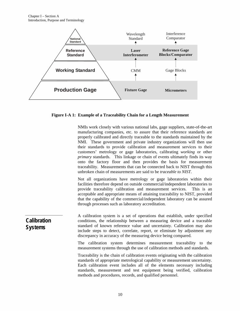
Figure I-A 1: Example of a Traceability Chain for a Length Measurement
NMIs work closely with various national labs, gage suppliers, state-of-the-art manufacturing companies, etc. to assure that their reference standards are properly calibrated and directly traceable to the standards maintained by the NMI. These government and private industry organizations will then use their standards to provide calibration and measurement services to their customers’ metrology or gage laboratories, calibrating working or other primary standards. This linkage or chain of events ultimately finds its way onto the factory floor and then provides the basis for measurement traceability. Measurements that can be connected back to NIST through this unbroken chain of measurements are said to be traceable to NIST.
Not all organizations have metrology or gage laboratories within their facilities therefore depend on outside commercial/independent laboratories to provide traceability calibration and measurement services. This is an acceptable and appropriate means of attaining traceability to NIST, provided that the capability of the commercial/independent laboratory can be assured through processes such as laboratory accreditation.
A calibration system is a set of operations that establish, under specified conditions, the relationship between a measuring device and a traceable standard of known reference value and uncertainty. Calibration may also include steps to detect, correlate, report, or eliminate by adjustment any discrepancy in accuracy of the measuring device being compared.
The calibration system determines measurement traceability to the measurement systems through the use of calibration methods and standards.
Traceability is the chain of calibration events originating with the calibration standards of appropriate metrological capability or measurement uncertainty. Each calibration event includes all of the elements necessary including standards, measurement and test equipment being verified, calibration methods and procedures, records, and qualified personnel.
Wavelength Standard
LaserInterferometer
Reference GageBlocks/Comparator
CMM Gage Blocks
Micrometers
InterferenceComparator
Fixture Gage
Working Standard
Reference Standard
NationalStandard
Production Gage
Calibration Systems
Chapter I – Section A Introduction, Purpose and Terminology
11
True Value
An organization may have an internal calibration laboratory or organization which controls and maintains the elements of the calibration events. These internal laboratories will maintain a laboratory scope which lists the specific calibrations they are capable of performing as well as the equipment and methods/procedures used to perform the calibrations.
The calibration system is part of an organization’s quality management system and therefore should be included in any internal audit requirements.
Measurement Assurance Programs (MAPs) can be used to verify the acceptability of the measurement processes used throughout the calibration system. Generally MAPs will include verification of a measurement system’s results through a secondary independent measurement of the same feature or parameter. Independent measurements imply that the traceability of the secondary measurement process is derived from a separate chain of calibration events from those used for the initial measurement. MAPs may also include the use of statistical process control (SPC) to track the long-term stability of a measurement process.
Note: ANSI/NCSL Z540.3 and ISO 10012 each provide models for many of the elements of a calibration system.
When the calibration event is performed by an external, commercial, or independent calibration service supplier, the service supplier’s calibration system can (or may) be verified through accreditation to ISO/IEC 17025. When a qualified laboratory is not available for a given piece of equipment, calibration services may be performed by the equipment manufacturer.
The measurement process TARGET is the “true” value of the part. It is desired that any individual reading be as close to this value as (economically) possible. Unfortunately, the true value can never be known with certainty. However, uncertainty can be minimized by using a reference value based on a well defined operational definition of the characteristic, and using the results of a measurement system that has higher order discrimination and traceable to NIST. Because the reference value is used as a surrogate for the true value, these terms are commonly used interchangeably. This usage is not recommended.

Chapter I – Section A Introduction, Purpose and Terminology
12
Chapter I – Section B The Measurement Process
13
Section B The Measurement Process P
3
Measurement Systems
In order to effectively manage variation of any process, there needs to be knowledge of:
What the process should be doing
What can go wrong
What the process is doing
Specifications and engineering requirements define what the process should be doing.
The purpose of a Process Failure Mode Effects Analysis P
4F (PFMEA) is to
define the risk associated with potential process failures and to propose corrective action before these failures can occur. The outcome of the PFMEA is transferred to the control plan.
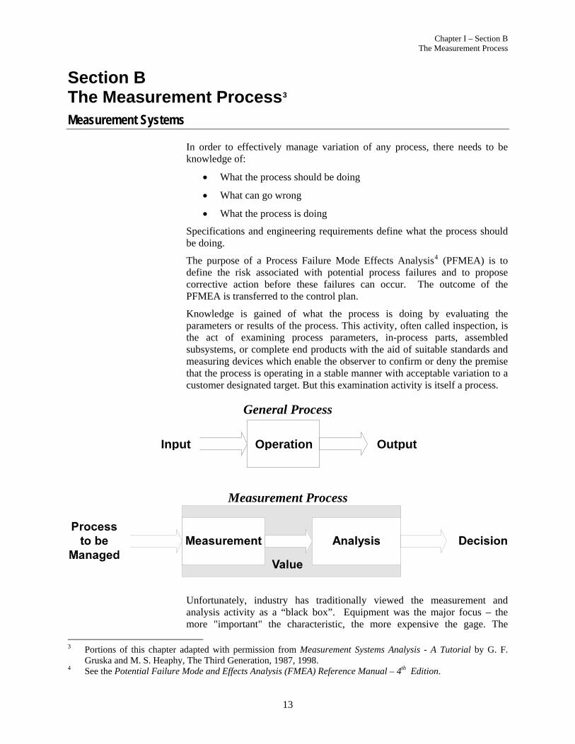
Knowledge is gained of what the process is doing by evaluating the parameters or results of the process. This activity, often called inspection, is the act of examining process parameters, in-process parts, assembled subsystems, or complete end products with the aid of suitable standards and measuring devices which enable the observer to confirm or deny the premise that the process is operating in a stable manner with acceptable variation to a customer designated target. But this examination activity is itself a process.
General Process
Measurement Process
Unfortunately, industry has traditionally viewed the measurement and analysis activity as a “black box”. Equipment was the major focus – the more "important" the characteristic, the more expensive the gage. The
3 Portions of this chapter adapted with permission from Measurement Systems Analysis - A Tutorial by G. F.
Gruska and M. S. Heaphy, The Third Generation, 1987, 1998. 4 See the Potential Failure Mode and Effects Analysis (FMEA) Reference Manual – 4th Edition.
OperationInput Output
Chapter I – Section B The Measurement Process
14
usefulness of the instrument, its compatibility with the process and environment, and its usability was rarely questioned. Consequently these gages were often not used properly or simply not used.
The measurement and analysis activity is a process – a measurement process. Any and all of the management, statistical, and logical techniques of process control can be applied to it.
This means that the customers and their needs must first be identified. The customer, the owner of the process, wants to make a correct decision with minimum effort. Management must provide the resources to purchase equipment which is necessary and sufficient to do this. But purchasing the best or the latest measurement technology will not necessarily guarantee correct production process control decisions.
Equipment is only one part of the measurement process. The owner of the process must know how to correctly use this equipment and how to analyze and interpret the results. Management must therefore also provide clear operational definitions and standards as well as training and support. The owner of the process has, in turn, the obligation to monitor and control the measurement process to assure stable and correct results which includes a total measurement systems analysis perspective – the study of the gage, procedure, user, and environment; i.e., normal operating conditions.
An ideal measurement system would produce only “correct” measurements each time it is used. Each measurement would always agree with a standard. P
5F
A measurement system that could produce measurements like that would be said to have the statistical properties of zero variance, zero bias, and zero probability of misclassifying any product it measured. Unfortunately, measurement systems with such desirable statistical properties seldom exist, and so process managers are typically forced to use measurement systems that have less desirable statistical properties. The quality of a measurement system is usually determined solely by the statistical properties of the data it produces over time. Other properties, such as cost, ease of use, etc., are also important in that they contribute to the overall desirability of a measurement system. But it is the statistical properties of the data produced that determine the quality of the measurement system.
Statistical properties that are most important for one use are not necessarily the most important properties for another use. For instance, for some uses of a coordinate measuring machine (CMM), the most important statistical properties are “small” bias and variance. A CMM with those properties will generate measurements that are “close” to the certified values of standards that are traceable. Data obtained from such a machine can be very useful for analyzing a manufacturing process. But, no matter how “small” the bias and variance of the CMM may be, the measurement system which uses the CMM may be unable to do an acceptable job of discriminating between good and bad product because of the additional sources of variation introduced by the other elements of the measurement system.
5 For a fuller discussion on the matter of standards see Out of the Crisis, W. Edwards Deming, 1982, 1986, p.
279-281.
Statistical Properties of Measurement Systems
Chapter I – Section B The Measurement Process
15
Management has the responsibility for identifying the statistical properties that are the most important for the ultimate use of the data. Management is also responsible for ensuring that those properties are used as the basis for selecting a measurement system. To accomplish this, operational definitions of the statistical properties, as well as acceptable methods of measuring them, are required. Although each measurement system may be required to have different statistical properties, there are certain fundamental properties that define a “good” measurement system. These include:
1) Adequate discrimination and sensitivity. The increments of measure
should be small relative to the process variation or specification limits for the purpose of measurement. The commonly known Rule of Tens, or 10-to-1 Rule, states that instrument discrimination should divide the tolerance (or process variation) into ten parts or more. This rule of thumb was intended as a practical minimum starting point for gage selection.
2) The measurement system ought to be in statistical control.FP6PF This means that under repeatable conditions, the variation in the measurement system is due to common causes only and not due to special causes. This can be referred to as statistical stability and is best evaluated by graphical methods.
3) For product control, variability of the measurement system must be small compared to the specification limits. Assess the measurement system to the feature tolerance.
4) For process control, the variability of the measurement system ought to demonstrate effective resolution and be small compared to manufacturing process variation. Assess the measurement system to the 6-sigma process variation and/or Total Variation from the MSA study.
The statistical properties of the measurement system may change as the items being measured vary. If so, then the largest (worst) variation of the measurement system is small relative to the smaller of either the process variation or the specification limits.
Similar to all processes, the measurement system is impacted by both random and systematic sources of variation. These sources of variation are due to common and special causes. In order to control the measurement system variation:
1) Identify the potential sources of variation.
2) Eliminate (whenever possible) or monitor these sources of variation.
Although the specific causes will depend on the situation, some typical sources of variation can be identified. There are various methods of
6 The measurement analyst must always consider practical and statistical significance.
Sources of Variation
Chapter I – Section B The Measurement Process
16
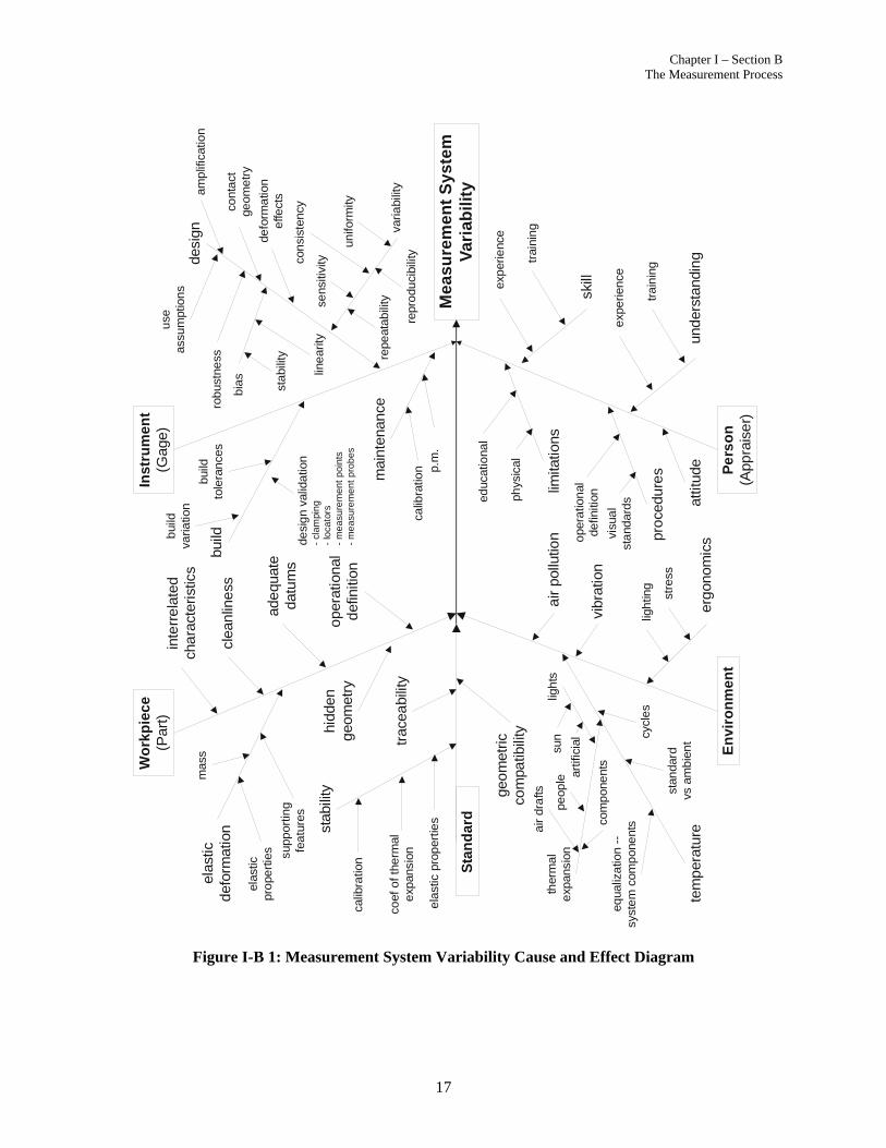
presenting and categorizing these sources of variation such as cause-effect diagrams, fault tree diagrams, etc., but the guidelines presented here will focus on the major elements of a measuring system.
The acronym S.W.I.P.E. P
7F is used to represent the six essential elements of a
generalized measuring system to assure attainment of required objectives. S.W.I.P.E. stands for Standard, Workpiece, Instrument, Person and Procedure, and Environment. This may be thought of as an error model for a complete measurement system. P
8
Factors affecting those six areas need to be understood so they can be controlled or eliminated.
Figure I-B 1 displays a cause and effect diagram showing some of the potential sources of variation. Since the actual sources of variation affecting a specific measurement system will be unique to that system, this figure is presented as a thought starter for developing a measurement system’s sources of variation.
7 TThis acronym was originally developed by Ms. Mary Hoskins, a metrologist associated with Honeywell, Eli Whitney Metrology Lab and the Bendix Corporation.T 8 See Appendix F for an alternate error model, P.I.S.M.O.E.A.
S Standard W Workpiece (i.e., part) I Instrument P Person / Procedure E Environment
Chapter I – Section B The Measurement Process
17
Figure I-B 1: Measurement System Variability Cause and Effect Diagram
Mea
sure
men
t S
yst
emV
aria
bil
ity
Sta
nd
ard
Wo
rkp
iece
(Par
t)In
stru
men
t(G
age)
En
viro
nm
ent
Pe
rso
n(A
ppra
iser)
geom
etric
com
patib
ility
coef
of t
herm
ale
xpan
sion
ela
stic
pro
per
ties
calib
ratio
n
stab
ility
elas
ticdef
orm
atio
n
supp
ortin
gfe
atu
res
elas
ticpr
ope
rtie
s
mas
s
clea
nlin
ess
inte
rrela
ted
cha
ract
eris
tics
hidd
engeo
met
ryope
ratio
nal
def
initi
on
ade
quat
eda
tum
s
skill
limita
tions
exp
erie
nce
trai
nin
g
under
stan
ding
train
ing
exp
erie
nce
attit
ude
phys
ical
educ
atio
nal
vibr
atio
n
tem
per
atur
e
stan
dard
vs a
mb
ien
t
equa
liza
tion
--
syst
em
com
pon
ent
s
trac
eabi
lity
air
pollu
tion
ergon
omic
s
ligh
ting
stre
ss
cycl
es
ther
ma
le
xpan
sion
sun
com
pon
ent
s
air
dra
fts
peop
lelig
hts
artif
icia
l
desi
gnam
plif
icat
ion
cont
act
geom
etr
y
defo
rma
tion
effe
cts
build
mai
nte
nance
bia
s
varia
bilit
y
stabi
lity
line
arity
repe
atab
ility
repr
odu
cibi
lity
sens
itivi
tycon
sist
ency
unifo
rmity
calib
ratio
n p.m
.
proce
dure
s
visu
al
sta
ndar
ds
ope
ratio
nal
defin
ition
bui
ldva
riatio
n
build
tole
ran
ces
desi
gn
valid
atio
n-
clam
pin
g-
loca
tors
- m
eas
ure
men
t poi
nts
- m
eas
ure
men
t pro
bes
rob
ustn
ess
use
assu
mpt
ion
s
Chapter I – Section B The Measurement Process
18
The Effects of Measurement System Variability
Because the measurement system can be affected by various sources of variation, repeated readings on the same part do not yield the same, identical result. Readings vary from each other due to common and special causes.
The effects of the various sources of variation on the measurement system should be evaluated over a short and long period of time. The measurement system capability is the measurement system (random) error over a short period of time. It is the combination of errors quantified by linearity, uniformity, repeatability and reproducibility. The measurement system performance, as with process performance, is the effect of all sources of variation over time. This is accomplished by determining whether our process is in statistical control (i.e., stable and consistent; variation is due only to common causes), on target (no bias), and has acceptable variation (gage repeatability and reproducibility (GRR)) over the range of expected results. This adds stability and consistency to the measurement system capability.
Because the output of the measurement system is used in making a decision about the product and the process, the cumulative effect of all the sources of variation is often called measurement system error, or sometimes just “error.”
After measuring a part, one of the actions that can be taken is to determine the status of that part. Historically, it would be determined if the part were acceptable (within specification) or unacceptable (outside specification). Another common scenario is the classification of parts into specific categories (e.g., piston sizes).
For the rest of the discussion, as an example, the two category situation will be used: out of specification (“bad”) and in specification (“good”). This does not restrict the application of the discussion to other categorization activities.
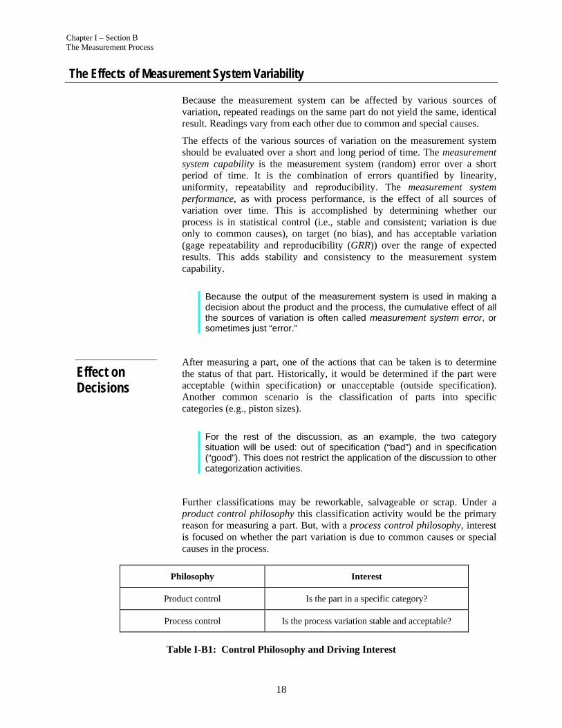
Further classifications may be reworkable, salvageable or scrap. Under a product control philosophy this classification activity would be the primary reason for measuring a part. But, with a process control philosophy, interest is focused on whether the part variation is due to common causes or special causes in the process.
Philosophy Interest
Product control Is the part in a specific category?
Process control Is the process variation stable and acceptable?
Table I-B1: Control Philosophy and Driving Interest
Effect on Decisions

Chapter I – Section B The Measurement Process
19
The next section deals with the effect of the measurement error on the product decision. Following that is a section which addresses its impact on the process decision.
In order to better understand the effect of measurement system error on product decisions, consider the case where all of the variability in multiple readings of a single part is due to the gage repeatability and reproducibility. That is, the measurement process is in statistical control and has zero bias.
A wrong decision will sometimes be made whenever any part of the above measurement distribution overlaps a specification limit. For example, a good part will sometimes be called “bad” (type I error, producer's risk or false alarm) if:
And, a bad part will sometimes be called “good” (type II error, consumer’s risk or miss rate) if:
NOTE: False Alarm Rate + Miss Rate = Error Rate.
RISK is the chance of making a decision which will be detrimental to an individual or process
That is, with respect to the specification limits, the potential to make the wrong decision about the part exists only when the measurement system error intersects the specification limits. This gives three distinct areas:
Effect on Product Decisions
Chapter I – Section B The Measurement Process
20
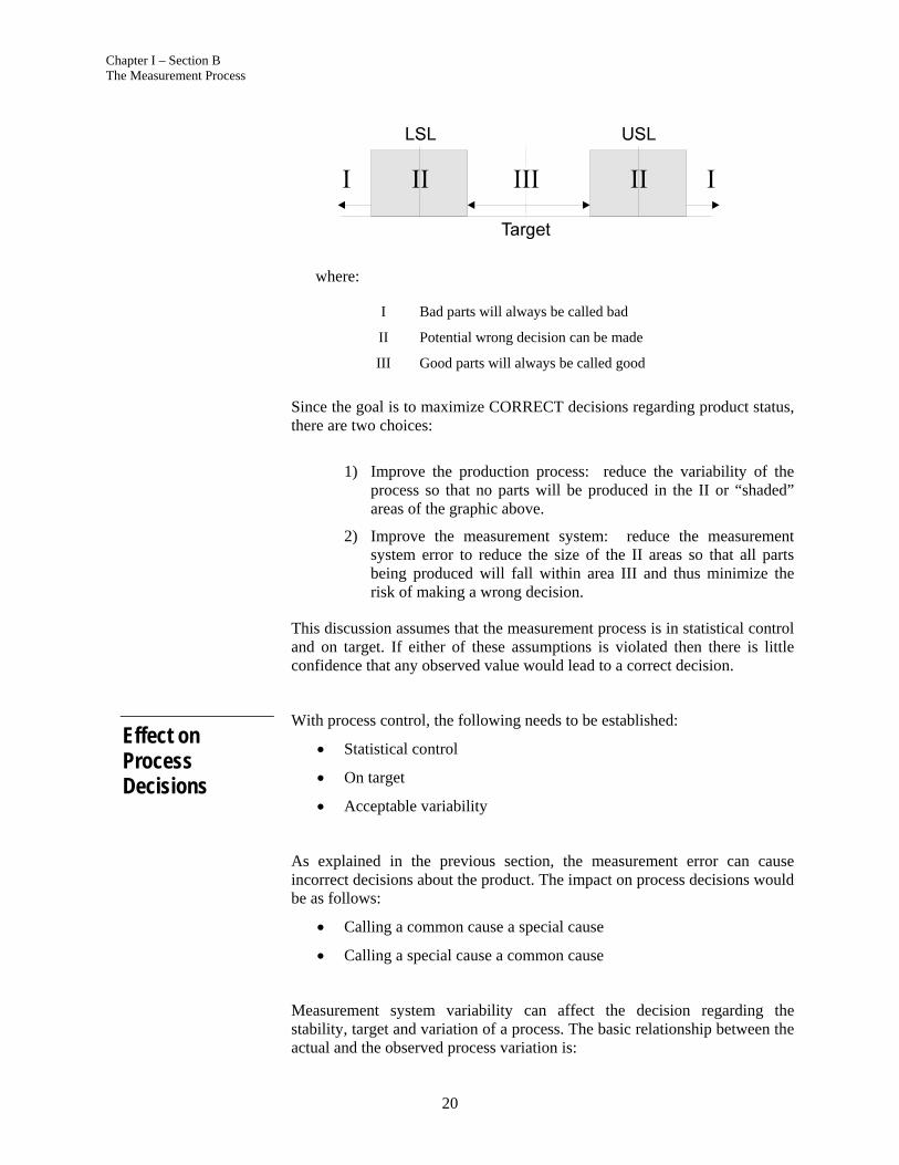
where:
I Bad parts will always be called bad
II Potential wrong decision can be made
III Good parts will always be called good
Since the goal is to maximize CORRECT decisions regarding product status, there are two choices:
1) Improve the production process: reduce the variability of the
process so that no parts will be produced in the II or “shaded” areas of the graphic above.
2) Improve the measurement system: reduce the measurement system error to reduce the size of the II areas so that all parts being produced will fall within area III and thus minimize the risk of making a wrong decision.
This discussion assumes that the measurement process is in statistical control and on target. If either of these assumptions is violated then there is little confidence that any observed value would lead to a correct decision.
With process control, the following needs to be established:
Statistical control
On target
Acceptable variability
As explained in the previous section, the measurement error can cause incorrect decisions about the product. The impact on process decisions would be as follows:
Calling a common cause a special cause
Calling a special cause a common cause
Measurement system variability can affect the decision regarding the stability, target and variation of a process. The basic relationship between the actual and the observed process variation is:
Effect on Process Decisions
Chapter I – Section B The Measurement Process
21
2 2 2obs actual msa
where
2obs = observed process variance
2actual = actual process variance
2msa = variance of the measurement system
The capability index P
9F Cp is defined as
6
ToleranceRangeCp
The relationship between the Cp index of the observed process and the Cp indices of the actual process and the measurement system is derived by substituting the equation for Cp into the observed variance equation above:
2 2 2
obs actual msaCp Cp Cp
Assuming the measurement system is in statistical control and on target, the actual process Cp can be compared graphically to the observed Cp. P
10F
Therefore the observed process capability is a combination of the actual process capability plus the variation due to the measurement process. To reach a specific process capability goal would require factoring in the measurement variation.
For example, if the measurement system Cp index were 2, the actual process would require a Cp index greater than or equal to 1.79 in order for the calculated (observed) index to be 1.33. If the measurement system Cp index were itself 1.33, the process would require no variation at all if the final result were to be 1.33 – clearly an impossible situation.
9 Although this discussion is using Cp, the results hold also for the performance index Pp. 10 See Appendix B for formulas and graphs.
Chapter I – Section B The Measurement Process
22
When a new process such as machining, manufacturing, stamping, material handling, heat treating, or assembly is purchased, there often is a series of steps that are completed as part of the buy-off activity. Oftentimes this involves some studies done on the equipment at the supplier's location and then at the customer's location.
If the measurement system used at either location is not consistent with the measurement system that will be used under normal circumstances then confusion may ensue. The most common situation involving the use of different instruments is the case where the instrument used at the supplier has higher order discrimination than the production instrument (gage). For example, parts measured with a coordinate measuring machine during buy-off and then with a height gage during production; samples measured (weighed) on an electronic scale or laboratory mechanical scale during buy-off and then on a simple mechanical scale during production.
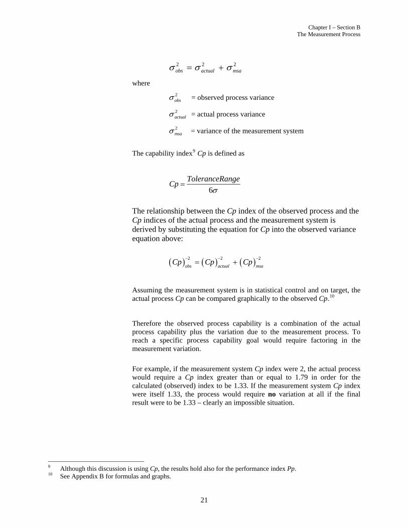
In the case where the (higher order) measurement system used during buy-off has a GRR of 10% and the actual process Cp is 2.0 the observed process Cp during buy-off will be 1.96. P
11F
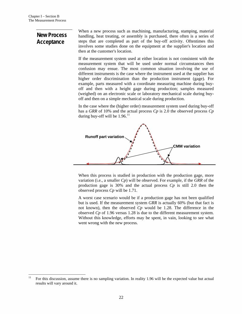
When this process is studied in production with the production gage, more variation (i.e., a smaller Cp) will be observed. For example, if the GRR of the production gage is 30% and the actual process Cp is still 2.0 then the observed process Cp will be 1.71.
A worst case scenario would be if a production gage has not been qualified but is used. If the measurement system GRR is actually 60% (but that fact is not known), then the observed Cp would be 1.28. The difference in the observed Cp of 1.96 versus 1.28 is due to the different measurement system. Without this knowledge, efforts may be spent, in vain, looking to see what went wrong with the new process.
11 For this discussion, assume there is no sampling variation. In reality 1.96 will be the expected value but actual
results will vary around it.
Runoff part variation
CMM variation
New Process Acceptance
Chapter I – Section B The Measurement Process
23
Often manufacturing operations use a single part at the beginning of the day to verify that the process is targeted. If the part measured is off target, the process is then adjusted. Later, in some cases another part is measured and again the process may be adjusted. Dr. Deming referred to this type of measurement and decision-making as tampering.
Consider a situation where the weight of a precious metal coating on a part is being controlled to a target of 5.00 grams. Suppose that the results from the scale used to determine the weight vary 0.20 grams but this is not known since the measurement system analysis was never done. The operating instructions require the operator to verify the weight at setup and every hour based on one sample. If the results are beyond the interval 4.90 to 5.10 grams then the operator is to setup the process again.
At setup, suppose the process is operating at 4.95 grams but due to measurement error the operator observes 4.85 grams. According to instructions the operator attempts to adjust the process up by .15 grams. Now the process is running at 5.10 grams for a target. When the operator checks the setup this time, 5.08 grams is observed so the process is allowed to run. Over-adjustment of the process has added variation and will continue to do so.
This is one example of the funnel experiment that Dr. Deming used to describe the effects of tampering. P
12F The measurement error just compounds
the problem.
Four rules of the funnel experiment are:
Rule 1: Make no adjustment or take no action unless the process is unstable.
Rule 2: Adjust the process in an equal amount and in an opposite direction from where the process was last measured to be.
Rule 3: Reset the process to the target. Then adjust the process in an equal amount and in an opposite direction from the target.
Rule 4: Adjust the process to the point of the last measurement.
The setup instruction for the precious metal process is an example of Rule 3. Rules 2, 3 and 4 add progressively more variation. Rule 1 is the best choice to produce minimum variation.
12 Deming, W. Edwards, Out of the Crisis, Massachusetts Institute of Technology, 1982, 1986.
Actual process variation
Production gage variationObserved process variation
Process Setup/ Control (Funnel Experiment)
Chapter I – Section B The Measurement Process
24
Other examples of the funnel experiment are:
Recalibration of gages based on arbitrary limits – i.e., limits not reflecting the measurement system’s variability. (Rule 3)
(Re)mastering the process control measurement system after an arbitrary number of uses without any indication or history of a change (special cause). (Rule 3)
Autocompensation adjusts the process based on the last part produced. (Rule 2)
On the job training (OJT) where worker A trains worker B who later trains worker C... without standard training material. Similar to the “post office” game. (Rule 4)
Parts are measured, found to be off target, but when plotted on a control chart the process is shown to be stable – therefore, no action is taken. (Rule 1)

Chapter I – Section C Measurement Strategy and Planning
25
Section C Measurement Strategy and Planning
Planning is key before designing and purchase of measurement equipment or systems. Many decisions made during the planning stage could affect the direction and selection of measurement equipment. What is the purpose and how will the measurement result be used? The planning stage will set the course and have a significant effect on how well the measurement process operates and can reduce possible problems and measurement error in the future.
In some cases due to the risk involved in the component being measured or because of the cost and complexity of the measurement device, the OEM customer may use the APQP process and committee to decide on the measurement strategy at the supplier.
Not all product and process characteristics require measurement systems whose development falls under this type of scrutiny. Simple standard measurement tools like micrometers or calipers may not require this in-depth strategy and planning. A basic rule of thumb is whether the characteristic being measured on the component or sub-system has been identified in the control plan or is important in determining the acceptance of the product or process. Another guide would be the level of tolerance assigned to a specific dimension. Common sense is the guide in any case.
The type, complexity, and purpose of a measurement system may drive various levels of program management, strategic planning, measurement systems analysis, or other special consideration for measurement selection, assessment and control. Simple measuring tools and devices (i.e., scales, measuring tapes, fixed-limit or attribute gages) may not require the level of management, planning, or analysis that more complex or critical measuring systems demand (i.e., master or reference, CMM, test stand, automated on-line gaging, etc.). Any measurement system may require more or less strategic planning and scrutiny depending on a given product or process situation. The decision as to the appropriate level shall be left to the APQP team assigned to the measurement process and customer. The actual degree of involvement or implementation in many of the activities below should be driven by the particular measurement system, consideration of the supporting gage control and calibration system, profound process knowledge, and common sense.
Complexity

Chapter I – Section C Measurement Strategy and Planning
26
The first step is to establish the purpose for the measurement and how the measurement will be utilized. A cross-functional team organized early in the development of the measurement process is critical in accomplishing this task. Specific considerations are made in relation to audit, process control, product and process development and analysis of the “Measurement Life Cycle”.
The Measurement Life Cycle concept expresses the belief that the measurement methods may change over time as one learns and improves the process. For example, measurement may start on a product characteristic to establish stability and capability of the process. This may lead to an understanding of critical process control characteristics that directly affect the part characteristics. Dependency on part characteristic information becomes less and the sampling plan may be reduced to signify this understanding (five parts per hour sample reduced to one part per shift). Also, the method of measurement may change from a CMM measurement, to some form of attribute gaging. Eventually it may be found that very little part monitoring may be required as long as the process is maintained or measuring and monitoring the maintenance and tooling may be all that is needed. The level of measurement follows the level of process understanding.
Most of the measuring and monitoring could eventually end up at suppliers of incoming material. The same measurement, on the same characteristic, at the same area of the process, over an extensive period of time is evidence of a lack of learning or a stagnant measurement process.
Before a measurement system can be purchased, a detailed engineering concept of the measurement process is developed. Using the purpose developed above, a cross-functional team of individuals will develop a plan and concept for the measurement system required by the design. Here are some guidelines:
The team needs to evaluate the design of the subsystem or component and identify important characteristics. These are based on customer requirements and the functionality of the subsystem or component to the total system. If the important dimensions have been identified already, evaluate the ability to measure the characteristics. For example, if the important characteristic of a plastic injection molded component was on the mold parting line, the dimensional check would be difficult and measurement variation would be high.
One method to capture issues similar to these would be to use a FMEA process to analyze areas of risk in gage design both from an ability to measure to the part to the functionality gage (Design and Process FMEA). This would aid in the development of the maintenance and calibration plan.
Develop a flow chart showing critical process steps in the manufacturing or assembly of the part or subsystem. Identify key inputs and outputs to each step in the process. This will aid in the development of the measurement equipment criteria and requirements affected by the location in the process.
Identify the Purpose of the Measurement Process
Criteria for a Measurement Process Design Selection
Measurement Life Cycle

Chapter I – Section C Measurement Strategy and Planning
27
A measurement plan, a list of measurement types, comes out of this investigation. P
13
For complex measurement systems, a flow chart is made of the measurement process. This would include delivery of the part or sub-system being measured, the measurement itself, and the return of the part or sub-system to the process.
Next use some method of brainstorming with the group to develop general criteria for each measurement required. One of the simple methods to use is a cause and effect diagram. P
14F See the example in Figure I-B 1 as a thought
starter.
A few additional questions to consider in relation to measurement planning:
Who ought to be involved in the “needs” analysis? The flow chart and initial discussion will facilitate the identification of the key individuals.
Why will measurement be taken and how will it be used? Will the data be used for control, sorting, qualification, etc? The way the measurement will be used can change the sensitivity level of the measurement system.
What level of sensitivity will be required? What is the product specification? What is the expected process variability? How much of a difference between parts will the gage need to detect?
What type of information will be provided with the gage (e.g., manuals – operating, maintenance, etc.) and what basic operator skills are required? Who will do the training?
How are measurements taken? Will it be done manually, on a moving conveyor, off-line, automatically, etc? Are the part location and fixturing possible sources of variation? Contact or non-contact?
How will the measurement be calibrated and will it be compared with other measurement processes? Who will be responsible for the calibration masters?
When and where will the measurement be taken? Will the part be clean, oily, hot, etc.?
Remember to use data to substantiate common assumptions about the measurement process. It is better to be safe and collect data on the environment, rather than to make decisions based on the wrong information and having a system developed that is not robust to environmental issues.
13 This can be considered as a preliminary control plan. 14 See Guide to Quality Control, Kaoru Ishikawa, published by Asian Productivity Organization, 1986.
Chapter I – Section C Measurement Strategy and Planning
28
Current measurement methods should be researched prior to investing in new equipment. Proven measurement methods may provide more reliable operation. Where possible, use measurement equipment that has a proven track record.
Refer to “Suggested Elements for a Measurement System Development Checklist” at the end of Chapter I, Section D, when developing and designing concepts and proposals.
During and after the fabrication of the measurement equipment and development of the measurement process (methods, training, documentation, etc.), experimental studies and data collection activities will be performed. These studies and data will be used to understand this measurement process so that this process and future processes may be improved.
Research Various Measurement Process Methods
Develop and Design Concepts and Proposals

Chapter I – Section D Measurement Source Development
29
Section D Measurement Source Development
This section addresses the quotation/procurement timeframe of the life of a measurement process. It has been constructed to be a self-contained discussion about the process of developing a measurement process quotation package, obtaining responses to that package, awarding the project, completing final design, developing the measurement process, and, finally, marrying that measurement process to the production process for which it was created. It is strongly encouraged that this chapter not be used without reading and understanding the entire discussion about a measurement process. To obtain the most benefit from the measurement process, study and address it as a process with inputs and outputs. P
15
This chapter was written with the team philosophy in mind. It is not a job description for the buyer or purchasing agent. The activities described here will require team involvement to be completed successfully and it should be administered within the overall framework of an Advanced Product Quality Planning (APQP) team. This can result in healthy interplay between various team functions – concepts arising out of the planning process may be modified before the gage supplier arrives at a final design that satisfies the measurement system requirements.
Generally, the “acquisition process” begins with formal communication between the customer and supplier for a given project. Up-front communication is crucial to the success of the project, since the groundwork necessary for an effective future customer/supplier relationship will be done at this stage. The acquisition process begins with the customer’s formal presentation of the intent of the project in the form of a Request For Quote (RFQ) followed by the supplier’s formal explanation of their proposal to meet this intent (the Quotation). The customer and supplier(s) need to thoroughly understand the project requirements, what the deliverables will be and the methods by which both are to be achieved. This understanding is derived from accurate timely communication between the two parties.
Once a concept has been agreed upon and a customer/supplier relationship has been established for the project at hand, the detailed design, fabrication of the measurement process, and development activities can commence. Communication between the customer and the supplier at this time is especially important. Since there may be several levels of concept approvals to be carried out, and possible environmental changes and the potential of team members changing, the measurement process project could falter or even fail. This risk will be reduced if frequent, detailed communication is maintained and documented between the customer and supplier and formal responsibility (an individual) for maintaining communication is designated
15 See Chapter I, Section B
OUTPUT INPUT
MEASUREMENT PROCESS
Chapter I – Section D Measurement Source Development
30
Datum Coordination
by both parties. The ideal forum and format for this activity is the Advanced Product Quality Planning (APQP) process.
After the measurement process has been conceptually designed, the activities surrounding the acquisition of the process/system can begin.
Ideally, with the current prevalence in the use of Geometric Dimensioning & Tolerancing (GD&T), datums need to be coordinated (i.e., made identical) throughout the manufacturing process and the measurement system and this needs to be established very early in the APQP process. Initial responsibility for this may lie with the product design engineer, dimensional control, etc. depending on the specific organization. When datum schemes do not match throughout a manufacturing process, particularly in the measurement systems, this leads to a situation where the wrong things may be measured, and there may be fit problems, etc., leading to ineffective control of the manufacturing process.
There may be times when a datum scheme used in a final assembly cannot possibly match that used in a sub-component manufacturing process. When such is the case, it can be established as early as possible in the APQP process so that all team members understand possible difficulties and conflicts that may lie ahead and have every opportunity to do something about it. During this process, different datum schemes may need to be explored in order to understand the impact of these differences.
Certain commodities present features which can yield more problems than others, such as camshaft centering, or other round, cylindrical or tubular characteristics. For example, a camshaft must be manufactured on centers but the important product features are in its lobes. One method or datum scheme may be required for manufacturing whereas another scheme is required for measurement of the final product measurement.

Chapter I – Section D Measurement Source Development
31
Detailed Engineering Concept
Prerequisites and Assumptions
Before discussing the development of a gage supplier, it will be assumed that issues such as “correct” engineering product design (GD&T) and “correct” process design (one which allows for measurement at the proper time and location in the process) have been resolved. However this should not detract from consideration of these issues with appropriate team members early in the APQP process.
It is assumed that the gage supplier will be involved with the APQP process, a team approach. The gage supplier will develop a clear appreciation of the overall production process and product usage so that his role is understood not only by him but by others on the team (manufacturing, quality, engineering, etc.).
There may be slight overlap in some activities or the order of those activities depending on the particular program/project or other constraints. For instance, the APQP team without much input from a gage source may develop certain gage concepts. Other concepts may require the expertise of the gage source. This may be driven by the complexity of the measurement system and a team decision as to what makes sense.
Gage Source Selection Process
Develop the Quotation Package
Before a measurement process request for quotation package can be supplied to a potential supplier for formal proposals, a detailed engineering concept of the measurement process needs to be developed. The team of individuals that will employ and be responsible for the maintenance and continual improvement of the measurement process have direct responsibility for developing the detailed concept. This can be part of the APQP team. To better develop this concept, several questions need to be answered.
The team may research various issues to help decide which direction or path will be followed for designing the measurement process. Some may be dictated or heavily implied by the product design. Examples of the multitude of possible issues that need to be addressed by the team when developing this detailed concept may be found in the “Suggested Elements for a Measurement System Development Checklist” at the end of this section.

Chapter I – Section D Measurement Source Development
32
Preventive Maintenance Considerations
All too often, customers rely too heavily on suppliers for solutions. Before a customer asks a supplier to suggest solutions to process problems, the foundation and intent of the process needs to be thoroughly understood and anticipated by the team that owns that process. Then and only then will the process be properly used, supported and improved upon.
What activities should be scheduled for preventive maintenance (e.g., lubrication, vibration analysis, probe integrity, parts replacement, etc.)? Much of these activities will depend on the complexity of the measurement system, device or apparatus. Simpler gages may require only an inspection at regular intervals, whereas more complex systems may require ongoing detailed statistical analyses and a team of engineers to maintain in a predictive fashion.
Planning preventive maintenance activities should coincide with the initiation of the measurement process planning. Many activities, such as draining air filters daily, lubricating bearings after the designated number of operating hours, etc., can be planned before the measurement system is completely built, developed and implemented. In fact this is preferable and improves advanced measurement planning and costs. Data collection methods and maintenance recommendations related to these activities can be obtained from the original manufacturer, or developed by plant engineering, manufacturing and quality personnel. After the measurement process is implemented and in use, data pertaining to the function of the measurement process need to be collected and plotted over time. Simple analytical methods (run charts, trend analysis) can be conducted to determine the stability of the system. Eventually, as the judgment of system stability dictates, preventive maintenance routines can be scheduled accordingly. Conducting preventive maintenance on a stable system, based on time series information, will be less wasteful than conducting preventive maintenance on a system with traditional techniques.
Specifications serve as guidelines for both the customer and supplier in the design and build process. These guidelines serve to communicate acceptable standards. Acceptable standards may be considered in two categories:
Design Standards Build Standards
Format of the design standards may be different depending on who is paying for the project. Cost issues may affect the format. Generally, it is a good idea to have sufficient documented design detail that the design may be built or repaired to original intent by any qualified builder – however, this decision
Specifications
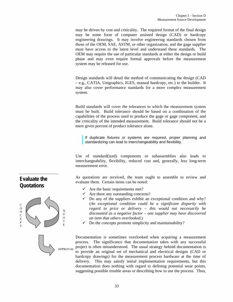
Chapter I – Section D Measurement Source Development
33
Q U O T E
C O N C E P T
APPROVAL
Evaluate the Quotations
may be driven by cost and criticality. The required format of the final design may be some form of computer assisted design (CAD) or hardcopy engineering drawings. It may involve engineering standards chosen from those of the OEM, SAE, ASTM, or other organization, and the gage supplier must have access to the latest level and understand these standards. The OEM may require the use of particular standards at either the design or build phase and may even require formal approvals before the measurement system may be released for use.
Design standards will detail the method of communicating the design (CAD – e.g., CATIA, Unigraphics, IGES, manual hardcopy, etc.) to the builder. It may also cover performance standards for a more complex measurement system.
Build standards will cover the tolerances to which the measurement system must be built. Build tolerance should be based on a combination of the capabilities of the process used to produce the gage or gage component, and the criticality of the intended measurement. Build tolerance should not be a mere given percent of product tolerance alone.
If duplicate fixtures or systems are required, proper planning and standardizing can lead to interchangeability and flexibility.
Use of standard(ized) components or subassemblies also leads to interchangeability, flexibility, reduced cost and, generally, less long-term measurement error.
As quotations are received, the team ought to assemble to review and evaluate them. Certain items can be noted:
Are the basic requirements met? Are there any outstanding concerns? Do any of the suppliers exhibit an exceptional condition and why?
(An exceptional condition could be a significant disparity with regard to price or delivery – this would not necessarily be discounted as a negative factor – one supplier may have discovered an item that others overlooked.)
Do the concepts promote simplicity and maintainability?
Documentation is sometimes overlooked when acquiring a measurement process. The significance that documentation takes with any successful project is often misunderstood. The usual strategy behind documentation is to provide an original set of mechanical and electrical designs (CAD or hardcopy drawings) for the measurement process hardware at the time of delivery. This may satisfy initial implementation requirements, but this documentation does nothing with regard to defining potential wear points, suggesting possible trouble areas or describing how to use the process. Thus,
Chapter I – Section D Measurement Source Development
34
the required documentation for any process ought to include more than assembly and detailed drawings of the measurement equipment.
Effective documentation for any system serves the same purpose as a good map on a trip. For example, it will suggest to the user how to get from one point to another (user instructions or gage instructions). It provides the user with possible alternative routes to reach the desired destinations (troubleshooting guides or diagnostic trees) if the main route is blocked or closed.
A complete documentation package may include:
Reproducible set of assembly and detailed mechanical drawings
(CAD or hardcopy) (including any required masters)
Reproducible set of electrical hard-wiring, logic and software
Suggested spare parts list of heavy use or wear items/details. This list should include items that may require considerable lead-time to acquire
Maintenance manuals with machine drawing cutaways and steps
to properly assemble and disassemble machine components
Manuals defining utility requirements for setup and operation and machine transport requirements (e.g., load bearing members)
Diagnostic trees and a troubleshooting guide
Certification reports (traceable to NIST where applicable)
Calibration instructions
User manuals that can be used by the technical support
personnel, the system operator and maintenance personnel
The above list can be used as a checklist when organizing the quotation package; however it is not necessarily all-inclusive.
The central theme here is communication. Since documentation is a form of communication, the team and others ought to be involved at every level of the development of the measurement process documentation package.
Chapter I – Section D Measurement Source Development
35
Shipment
Qualification at the Supplier
The gage or measurement system should be given a full dimensional layout and functional test, where applicable, at the measurement system supplier before shipment. Obviously, the chosen supplier must have qualified measurement equipment and personnel on site in order to accomplish this. If not, pre-arrangements should have been made to have this work done at an outside independent qualified laboratory. Results of such dimensional layout and/or testing should be done in accordance with customer design and build standards and be fully documented and available for customer review.
After successful dimensional layout, the supplier should perform a preliminary but formal measurement systems analysis. This again pre-requires that the supplier have the personnel, knowledge and experience to accomplish the appropriate analysis. The customer should predetermine with the supplier (and perhaps the OEM) exactly what sort of analysis is required at this point and should be aware of any guidance the supplier might need. Some issues that may need discussion, negotiation or common agreement are:
Objective of the preliminary MSA study :
Gage repeatability (GR P
16F) versus gage repeatability and
reproducibility (GRR) Assessment of bias and/or linearity Assessment of the customer purpose for measurement
Quantity of pieces, trials and operators in study
Acceptance criteria
Use of supplier personnel vs. customer supplied personnel
Necessary training for personnel
Are they qualified? Do they understand intent? What software might be used?Whatever results are
achieved at this point in time, it should be realized that these are merely preliminary and judgment may be needed as to the acceptability of the results.
CHECKLIST
When should the equipment be shipped?
How should it be shipped?
Who removes equipment from the truck or rail car?
Is insurance required?
Should documentation be shipped with the hardware?
Does the customer have the proper equipment to unload the hardware?
Where will the system be stored until shipment? 16 See Appendix D.
Chapter I – Section D Measurement Source Development
36
Documentation Delivery
Qualification at the Customer
Where will the system be stored until implementation?
Is the shipping documentation complete and easily understandable for the loader, transporter, unloader and installation crew?
Generally, what was done to qualify the measurement system above at the supplier before shipment should be repeated in some manner at the customer once delivery is completed. Since this becomes the first real opportunity to study the measurement system in its intended environment, acceptance standards and analysis methods used here should be considered seriously. Attention to detail on the part of all parties involved is paramount to the eventual success of this measurement system and the use of the data it generates.
Before any measurement analysis is begun after receipt, the measurement system should undergo a full dimensional layout to confirm it meets build requirements/standards. The extent of this layout may be balanced against layout work done previously at the measurement system supplier before shipment and confidence in the quality of the layout results done at the supplier as well as the lack of potential shipping damage. When comparing results before and after shipment, be aware that there will likely be some differences in these measurements because of differences in these measurement systems.
The information that is required, at a minimum, to aid implementation and startup of any system is the following: (This information ought to be delivered to the customer prior to delivery.)
CAD or hardcopy drawings, if required by team
Process flow diagram of the system, where applicable
User manuals
Maintenance/service manual Spare parts list Troubleshooting guide
Calibration instructions
Any special considerations
At the outset, the delivered documentation needs to be noted as preliminary. Original or reproducible documentation does not need to be delivered at this time because potential revision may be necessary after implementation. In fact, it is a wise idea to not have the original documentation package delivered until after the entire system is implemented – suppliers are generally more efficient with updating documentation than customers.
Chapter I – Section D Measurement Source Development
37
Suggested Elements for a Measurement System Development Checklist
This list should be modified based on the situation and type of measurement system. The development of the final checklist should be the result of collaboration between the customer and supplier.
Measurement System Design and Development Issues: What is to be measured? What type of characteristic is it? Is it a mechanical property? Is it dynamic or
stationary? Is it an electrical property? Is there significant within-part variation? For what purpose will the results (output) of the measurement process be used? Production improvement,
production monitoring, laboratory studies, process audits, shipping inspection, receiving inspection, responses to a D.O.E.?
Who will use the process? Operators, engineers, technicians, inspectors, auditors? Training required: Operator, maintenance personnel, engineers; classroom, practical application, OJT,
apprenticeship period. Have the sources of variation been identified? Build an error model (S.W.I.P.E. or P.I.S.M.O.E.A.) using
teams, brainstorming, profound process knowledge, cause & effect diagram or matrix. Has a FMEA been developed for the measurement system? Flexible vs. dedicated measurement systems: Measurement systems can either be permanent and dedicated
or they can be flexible and have the ability to measure different types of parts; e.g., doghouse gages, fixture gaging, coordinate measurement machine, etc. Flexible gaging will be more expensive, but can save money in the long run.
Contact vs. non-contact: Reliability, type of feature, sample plan, cost, maintenance, calibration, personnel
skill required, compatibility, environment, pace, probe types, part deflection, image processing . This may be determined by the control plan requirements and the frequency of the measurement ( Full contact gaging may get excessive wear during continuous sampling). Full surface contact probes, probe type, air feedback jets, image processing, CMM vs. optical comparator, etc.
Environment: Dirt, moisture, humidity, temperature, vibration, noise, electro-magnetic interference (EMI),
ambient air movement, air contaminants, etc. Laboratory, shop floor, office, etc? Environment becomes a key issue with low, tight tolerances in the micron level. Also, in cases that CMM, vision systems, ultrasonic, etc. This could be a factor in auto-feedback in-process type measurements. Cutting oils, cutting debris, and extreme temperatures could also become issues. Is a clean room required?
Measurement and location points: Clearly define, using GD&T, the location of fixturing and clamping points
and where on the part the measurements will be taken. Fixturing method: Free state versus clamped part holding. Part orientation: Body position versus other. Part preparation: Should the part be clean, non-oily, temperature stabilized, etc. before measurement? Transducer location: Angular orientation, distance from primary locators or nets.
Chapter I – Section D Measurement Source Development
38
Correlation issue #1 – duplicate gaging: Are duplicate (or more) gages required within or between plants to
support requirements? Building considerations, measurement error considerations, maintenance considerations. Which is considered the standard? How will each be qualified?
Correlations issue #2 – methods divergence: Measurement variation resulting from different measurement
system designs performing on the same product/process within accepted practice and operation limits (e.g., CMM versus manual or open-setup measurement results).
Automated vs. manual: on-line, off-line, operator dependencies. Destructive versus nondestructive measurement (NDT): Examples: tensile test, salt spray testing,
plating/paint coating thickness, hardness, dimensional measurement, image processing, chemical analysis, stress, durability, impact, torsion, torque, weld strength, electrical properties, etc.
Potential measurement range: size and expected range of conceivable measurements. Effective resolution: Is measurement sensitive to physical change (ability to detect process or product
variation) for a particular application acceptable for the application? Sensitivity: Is the size of the smallest input signal that results in a detectable (discernable) output signal for this
measurement device acceptable for the application? Sensitivity is determined by inherent gage design and quality (OEM), in-service maintenance, and operating condition.
Measurement System Build Issues (equipment, standard, instrument): Have the sources of variation identified in the system design been addressed? Design review; verify and
validate. Calibration and control system: Recommended calibration schedule and audit of equipment and
documentation. Frequency, internal or external, parameters, in-process verification checks. Input requirements: Mechanical, electrical, hydraulic, pneumatic, surge suppressors, dryers, filters, setup and
operation issues, isolation, discrimination and sensitivity. Output requirements: Analog or digital, documentation and records, file, storage, retrieval, backup. Cost: Budget factors for development, purchase, installation, operation and training. Preventive maintenance: Type, schedule, cost, personnel, training, documentation. Serviceability: Internal and external, location, support level, response time, availability of service parts,
standard parts list. Ergonomics: Ability to load and operate the machine without injuries over time. Measurement device
discussions need to focus on issues of how the measurement system is interdependent with the operator. Safety considerations: Personnel, operation, environmental, lock-out. Storage and location: Establish the requirements around the storage and location of the measurement
equipment. Enclosures, environment, security, availability (proximity) issues. Measurement cycle time: How long will it take to measure one part or characteristic? Measurement cycle
integrated to process and product control. Will there be any disruption to process flow, lot integrity, to capture, measure and return the part?
Chapter I – Section D Measurement Source Development
39
Material handling: Are special racks, holding fixtures, transport equipment or other material handling
equipment needed to deal with parts to be measured or the measurement system itself? Environmental issues: Are there any special environmental requirements, conditions, limitations, either
affecting this measurement process or neighboring processes? Is special exhausting required? Is temperature or humidity control necessary? Humidity, vibration, noise, EMI, cleanliness.
Are there any special reliability requirements or considerations? Will the equipment hold up over time?
Does this need to be verified ahead of production use? Spare parts: Common list, adequate supply and ordering system in place, availability, lead-times understood
and accounted for. Is adequate and secure storage available? (bearings, hoses, belts, switches, solenoids, valves, etc.)
User instructions: Clamping sequence, cleaning procedures, data interpretation, graphics, visual aids,
comprehensive. Available, appropriately displayed. Documentation: Engineering drawings, diagnostic trees, user manuals, language, etc. Calibration: Comparison to acceptable standards. Availability and cost of acceptable standards.
Recommended frequency, training requirements. Down-time required? Storage: Are there any special requirements or considerations regarding the storage of the measurement
device? Enclosures, environment, security from damage/theft, etc. Error/Mistake proofing: Can known measurement procedure mistakes be corrected easily (too easily?) by the
user? Data entry, misuse of equipment, error proofing, mistake proofing. Measurement System Implementation Issues (process):
Support: Who will support the measurement process? Lab technicians, engineers, production, maintenance, outside contracted service?
Training: What training will be needed for operators/inspectors/technicians/engineers to use and maintain this
measurement process? Timing, resource and cost issues. Who will train? Where will training be held? Lead-time requirements? Coordinated with actual use of measurement process.
Data management: How will data output from this measurement process be managed? Manual,
computerized, summary methods, summary frequency, review methods, review frequency, customer requirements, internal requirements. Availability, storage, retrieval, backup, security. Data interpretation.
Personnel: Will personnel need to be hired to support this measurement process? Cost, timing, availability
issues. Current or new. Improvement methods: Who will improve the measurement process over time? Engineers, production,
maintenance, quality personnel? What evaluation methods will be used? Is there a system to identify needed improvements?
Long-term stability: Assessment methods, format, frequency, and need for long-term studies. Drift, wear,
contamination, operational integrity. Can this long-term error be measured, controlled, understood, predicted? Special considerations: Inspector attributes, physical limitations or health issues: colorblindness, vision,
strength, fatigue, stamina, ergonomics.

Chapter I – Section D Measurement Source Development
40
Chapter I – Section E Measurement Issues
41
Section E Measurement Issues
Three fundamental issues must be addressed when evaluating a measurement system:
1) The measurement system must demonstrate adequate sensitivity.
First, does the instrument (and standard) have adequate discrimination? Discrimination (or class) is fixed by design and serves as the basic starting point for selecting a measurement system. Typically, the Rule of Tens has been applied, which states that instrument discrimination should divide the tolerance (or process variation) into ten parts or more.
Second, does the measurement system demonstrate effective resolution? Related to discrimination, determine if the measurement system has the sensitivity to detect changes in product or process variation for the application and conditions.
2) The measurement system must be stable.
Under repeatability conditions, the measurement system variation is due to common causes only and not special (chaotic) causes.
The measurement analyst must always consider practical and statistical significance.
3) The statistical properties (errors) are consistent over the expected
range and adequate for the purpose of measurement (product control or process control).
The long-standing tradition of reporting measurement error only as a percent of tolerance is inadequate for the challenges of the marketplace that emphasize strategic and continuous process improvement. As processes change and improve, a measurement system must be re-evaluated for its intended purpose. It is essential for the organization (management, measurement planner, production operator, and quality analyst) to understand the purpose of measurement and apply the appropriate evaluation.
Chapter I – Section E Measurement Issues
42
It is often assumed that measurements are exact, and frequently the analysis and conclusions are based upon this assumption. An individual may fail to realize there is variation in the measurement system which affects the individual measurements, and subsequently, the decisions based upon the data. Measurement system error can be classified into five categories: bias, repeatability, reproducibility, stability and linearity.
One of the objectives of a measurement system study is to obtain information relative to the amount and types of measurement variation associated with a measurement system when it interacts with its environment. This information is valuable, since for the average production process, it is far more practical to recognize repeatability and calibration bias and establish reasonable limits for these, than to provide extremely accurate gages with very high repeatability. Applications of such a study provide the following:
A criterion to accept new measuring equipment
A comparison of one measuring device against another
A basis for evaluating a gage suspected of being deficient
A comparison for measuring equipment before and after repair
A required component for calculating process variation, and the acceptability level for a production process
Information necessary to develop a Gage Performance Curve (GPC), P
17F which indicates the probability of accepting a part of some
true value
The following definitions help describe the types of error or variation associated with a measurement system, so that each term is clearly understood for subsequent discussion. An illustration is given for each definition which graphically displays the meaning of each term.
17 See Chapter V, Section C.
Types of Measurement System Variation
Chapter I – Section E Measurement Issues
43
Operational Definition
“An operational definition is one that people can do business with. An operational definition of safe, round, reliable, or any other quality [characteristic] must be communicable, with the same meaning to vendor as to the purchaser, same meaning yesterday and today to the production worker. Example:
1) A specific test of a piece of material or an assembly
2) A criterion (or criteria) for judgment
3) Decision: yes or no, the object or the material did or did not meet the criterion (or criteria)” FP18
Standard
A standard is anything taken by general consent as a basis for comparison; an accepted model. It can be an artifact or ensemble (instruments, procedures, etc.) set up and established by an authority as a rule for the measure of quantity, weight, extent, value or quality.
The concept of ensemble was formalized in ANSI/ASQC Standard M1-1996. P
19F This term was used to stress the fact that all of the influences
affecting the measurement uncertainty need to be taken into account; e.g., environment, procedures, personnel, etc. “An example of a simple ensemble would be an ensemble for the calibration of gage blocks consisting of a standard gage block, a comparator, an operator, environment, and the calibration procedure.”
Reference Standards
A standard, generally of the highest metrological quality available at a given location, from which measurements made at that location are derived.
Measurement and Test Equipment (M&TE)
All of the measurement instruments, measurement standards, reference materials, and auxiliary apparatus that are necessary to perform a measurement.
Calibration Standard
A standard that serves as a reference in the performance of routine calibrations. Intended to act as a buffer between the calibration workload and the laboratory’s reference standard(s).
18 W. E. Deming, Out of the Crisis (1982, 1986), p. 277. 19 This definition was later updated as Measurement and Test Equipment or M&TE by subsequent military
standards.
Definitions and Potential Sources of Variation
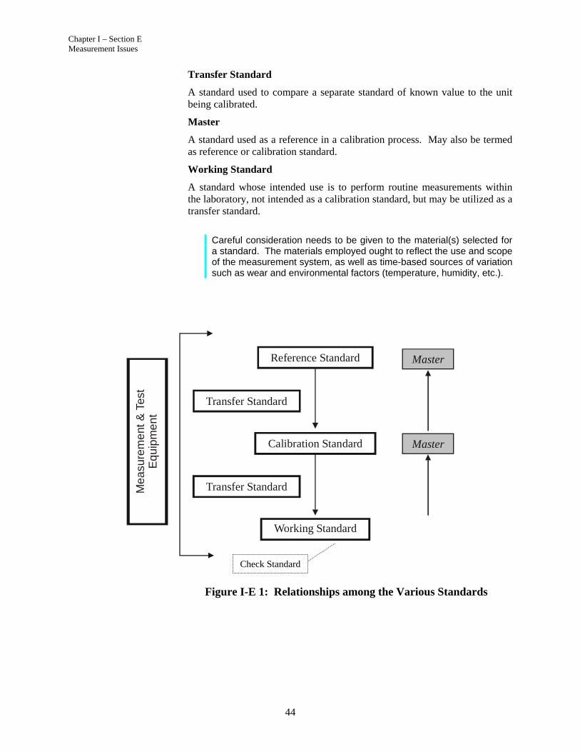
Chapter I – Section E Measurement Issues
44
Transfer Standard
A standard used to compare a separate standard of known value to the unit being calibrated.
Master
A standard used as a reference in a calibration process. May also be termed as reference or calibration standard.
Working Standard
A standard whose intended use is to perform routine measurements within the laboratory, not intended as a calibration standard, but may be utilized as a transfer standard.
Careful consideration needs to be given to the material(s) selected for a standard. The materials employed ought to reflect the use and scope of the measurement system, as well as time-based sources of variation such as wear and environmental factors (temperature, humidity, etc.).
Figure I-E 1: Relationships among the Various Standards
Reference Standard
Calibration Standard
Working Standard
Transfer Standard
Transfer Standard
Master
Master
Me
asu
rem
ent
& T
est
Eq
uip
me
nt
Check Standard

Chapter I – Section E Measurement Issues
45
Check Standard
A measurement artifact that closely resembles what the process is designed to measure, but is inherently more stable than the measurement process being evaluated.
Reference Value
A reference value, also known as the accepted reference value or master value, is a value of an artifact or ensemble that serves as an agreed upon reference for comparison. Accepted reference values are based upon the following:
Determined by averaging several measurements with a higher level (e.g., metrology lab or layout equipment) of measuring equipment
Legal values: defined and mandated by law
Theoretical values: based on scientific principles
Assigned values: based on experimental work (supported by sound theory) of some national or international organization
Consensus values: based on collaborative experimental work under the auspices of a scientific or engineering group; defined by a consensus of users such as professional and trade organizations
Agreement values: values expressly agreed upon by the affected parties
In all cases, the reference value needs to be based upon an operational definition and the results of an acceptable measurement system. To achieve this, the measuring system used to determine the reference value should include:
Instrument(s) with a higher order discrimination and a lower measurement system error than the systems used for normal evaluation
Be calibrated with standards traceable to the NIST or other NMI
True Value
The true value is the “actual” measure of the part. Although this value is unknown and unknowable, it is the target of the measurement process. Any individual reading ought to be as close to this value as (economically) possible. Unfortunately, the true value can never be known with certainty. The reference value is used as the best approximation of the true value in all analyses. Because the reference value is used as a surrogate for the true value, these terms are commonly used interchangeably. This usage is not recommended. P
20F
20 See also ASTM E177-90a.
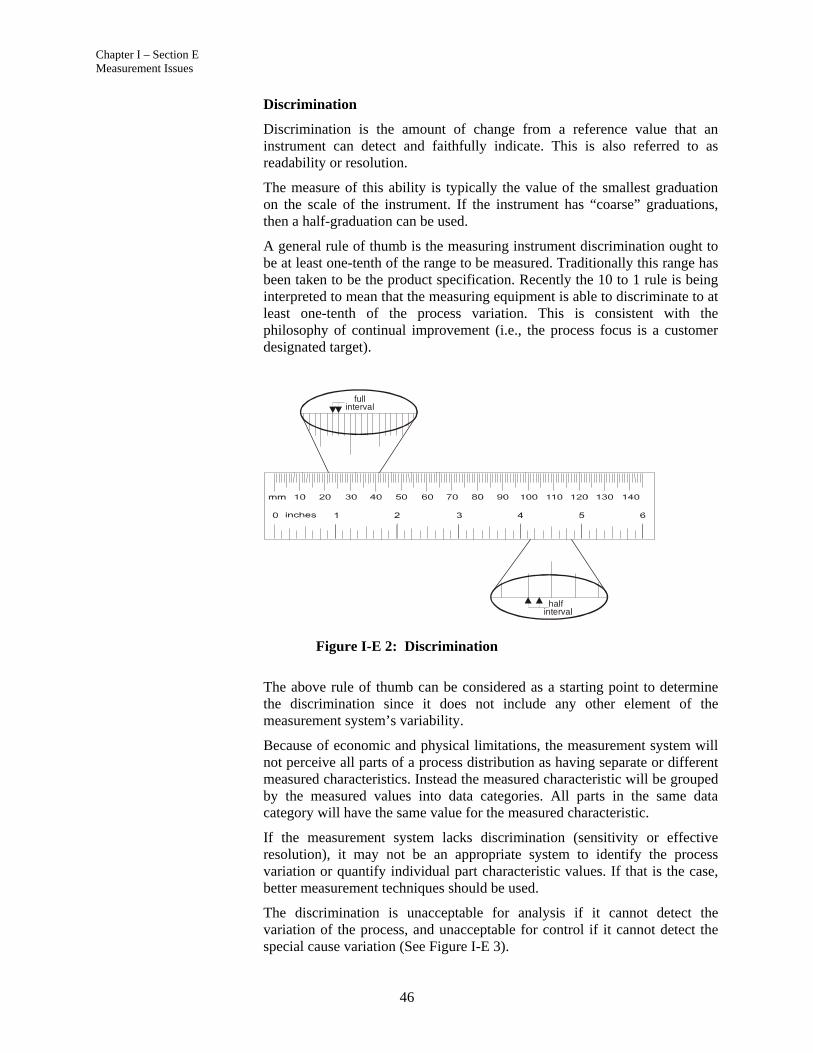
Chapter I – Section E Measurement Issues
46
Discrimination
Discrimination is the amount of change from a reference value that an instrument can detect and faithfully indicate. This is also referred to as readability or resolution.
The measure of this ability is typically the value of the smallest graduation on the scale of the instrument. If the instrument has “coarse” graduations, then a half-graduation can be used.
A general rule of thumb is the measuring instrument discrimination ought to be at least one-tenth of the range to be measured. Traditionally this range has been taken to be the product specification. Recently the 10 to 1 rule is being interpreted to mean that the measuring equipment is able to discriminate to at least one-tenth of the process variation. This is consistent with the philosophy of continual improvement (i.e., the process focus is a customer designated target).
Figure I-E 2: Discrimination
The above rule of thumb can be considered as a starting point to determine the discrimination since it does not include any other element of the measurement system’s variability.
Because of economic and physical limitations, the measurement system will not perceive all parts of a process distribution as having separate or different measured characteristics. Instead the measured characteristic will be grouped by the measured values into data categories. All parts in the same data category will have the same value for the measured characteristic.
If the measurement system lacks discrimination (sensitivity or effective resolution), it may not be an appropriate system to identify the process variation or quantify individual part characteristic values. If that is the case, better measurement techniques should be used.
The discrimination is unacceptable for analysis if it cannot detect the variation of the process, and unacceptable for control if it cannot detect the special cause variation (See Figure I-E 3).
halfinterval
fullinterval

Chapter I – Section E Measurement Issues
47
Number of Categories Control Analysis
Can be used for control only if: The process variation is small
when compared to the specifications
The loss function is flat over the expected process variation
The main source of variation causes a mean shift
Unacceptable for estimating
process parameters and indices Only indicates whether the
process is producing conforming or nonconforming parts
Can be used with semi-
variable control techniques based on the process distribution
Can produce insensitive variables control charts
Generally unacceptable for
estimating process parameters and indices since it only provides coarse estimates
Can be used with variables
control charts
Recommended
Figure I-E 3: Impact of Number of Distinct Categories (ndc) of the Process Distribution on Control and Analysis Activities
Symptoms of inadequate discrimination may appear in the range chart. Figure I-E 4 contains two sets of control charts derived from the same data. Control Chart (a) shows the original measurement to the nearest thousandth of an inch. Control Chart (b) shows these data rounded off to the nearest hundredth of an inch. Control Chart (b) appears to be out of control due to the artificially tight limits. The zero ranges are more a product of the rounding off than they are an indication of the subgroup variation.
A good indication of inadequate discrimination can be seen on the SPC range chart for process variation. In particular, when the range chart shows only one, two, or three possible values for the range within the control limits, the measurements are being made with inadequate discrimination. Also, if the range chart shows four possible values for the range within control limits and more than one-fourth of the ranges are zero, then the measurements are being made with inadequate discrimination. Another good indication of inadequate discrimination is on a normal probability plot where the data will be stacked into buckets instead of flowing along the 45 degree line.
5 or more Data Categories
2 - 4 Data Categories
1 Data Category
Chapter I – Section E Measurement Issues
48
Returning to Figure I-E 4, Control Chart (b), there are only two possible values for the range within the control limits (values of 0.00 and 0.01). Therefore, the rule correctly identifies the reason for the lack of control as inadequate discrimination (sensitivity or effective resolution).
This problem can be remedied, of course, by changing the ability to detect the variation within the subgroups by increasing the discrimination of the measurements. A measurement system will have adequate discrimination if its apparent resolution is small relative to the process variation. Thus a recommendation for adequate discrimination would be for the apparent resolution to be at most one-tenth of total process six sigma standard deviation instead of the traditional rule which is the apparent resolution be at most one-tenth of the tolerance spread.
Eventually, there are situations that reach a stable, highly capable process using a stable, “best-in-class” measurement system at the practical limits of technology. Effective resolution may be inadequate and further improvement of the measurement system becomes impractical. In these special cases, measurement planning may require alternative process monitoring techniques. Customer approval will typically be required for the alternative process monitoring technique.

Chapter I – Section E Measurement Issues
49
Figure I-E 4: Process Control Charts P
21
21 Figure I-E 4 was developed using data from Evaluating The Measurement Process, by Wheeler and Lyday,
Copyright 1989, SPC Press, Inc., Knoxville, Tennessee.
252015105Subgroup 0
0.145
0.140
0.135
Sa
mpl
eM
ea
n
Mean=0.1397
UCL=0.1444
LCL=0.1350
0.02
0.01
0.00
Sa
mpl
eR
ang
e
R=0.00812
UCL=0.01717
LCL=0
Xbar/R ChartDiscrimination = .001
252015105Subgroup 0
0.145
0.140
0.135Sa
mpl
eM
ea
n
Mean=0.1398
UCL=0.1438
LCL=0.1359
0.02
0.01
0.00
Sa
mpl
eR
ang
e
R=0.0068
UCL=0.01438
LCL=0
Xbar/R ChartDiscrimination = .01
B
A

Chapter I – Section E Measurement Issues
50
For most measurement processes, the total measurement variation is usually described as a normal distribution. Normal probability is an assumption of the standard methods of measurement systems analysis. In fact, there are measurement systems that are not normally distributed. When this happens, and normality is assumed, the MSA method may overestimate the measurement system error. The measurement analyst must recognize and correct evaluations for non-normal measurement systems.
Figure I-E 5: Characteristics of the Measurement Process Variation
Accuracy
Accuracy is a generic concept of exactness related to the closeness of agreement between the average of one or more measured results and a reference value. The measurement process must be in a state of statistical control, otherwise the accuracy of the process has no meaning.
In some organizations accuracy is used interchangeably with bias. The ISO (International Organization for Standardization) and the ASTM (American Society for Testing and Materials) use the term accuracy to embrace both bias and repeatability. In order to avoid confusion which could result from using the word accuracy, ASTM recommends that only the term bias be used as the descriptor of location error. This policy will be followed in this text.
Bias
Bias is often referred to as “accuracy.” Because “accuracy” has several meanings in literature, its use as an alternate for “bias” is not recommended.
Location Variation
Measurement Process Variation
Location
Width
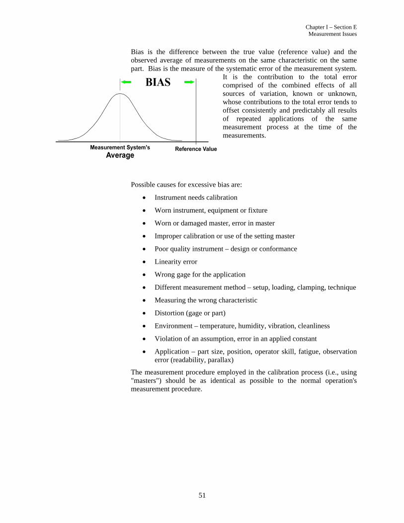
Chapter I – Section E Measurement Issues
51
Bias is the difference between the true value (reference value) and the observed average of measurements on the same characteristic on the same part. Bias is the measure of the systematic error of the measurement system.
It is the contribution to the total error comprised of the combined effects of all sources of variation, known or unknown, whose contributions to the total error tends to offset consistently and predictably all results of repeated applications of the same measurement process at the time of the measurements.
Possible causes for excessive bias are:
Instrument needs calibration
Worn instrument, equipment or fixture
Worn or damaged master, error in master
Improper calibration or use of the setting master
Poor quality instrument – design or conformance
Linearity error
Wrong gage for the application
Different measurement method – setup, loading, clamping, technique
Measuring the wrong characteristic
Distortion (gage or part)
Environment – temperature, humidity, vibration, cleanliness
Violation of an assumption, error in an applied constant
Application – part size, position, operator skill, fatigue, observation error (readability, parallax)
The measurement procedure employed in the calibration process (i.e., using "masters") should be as identical as possible to the normal operation's measurement procedure.
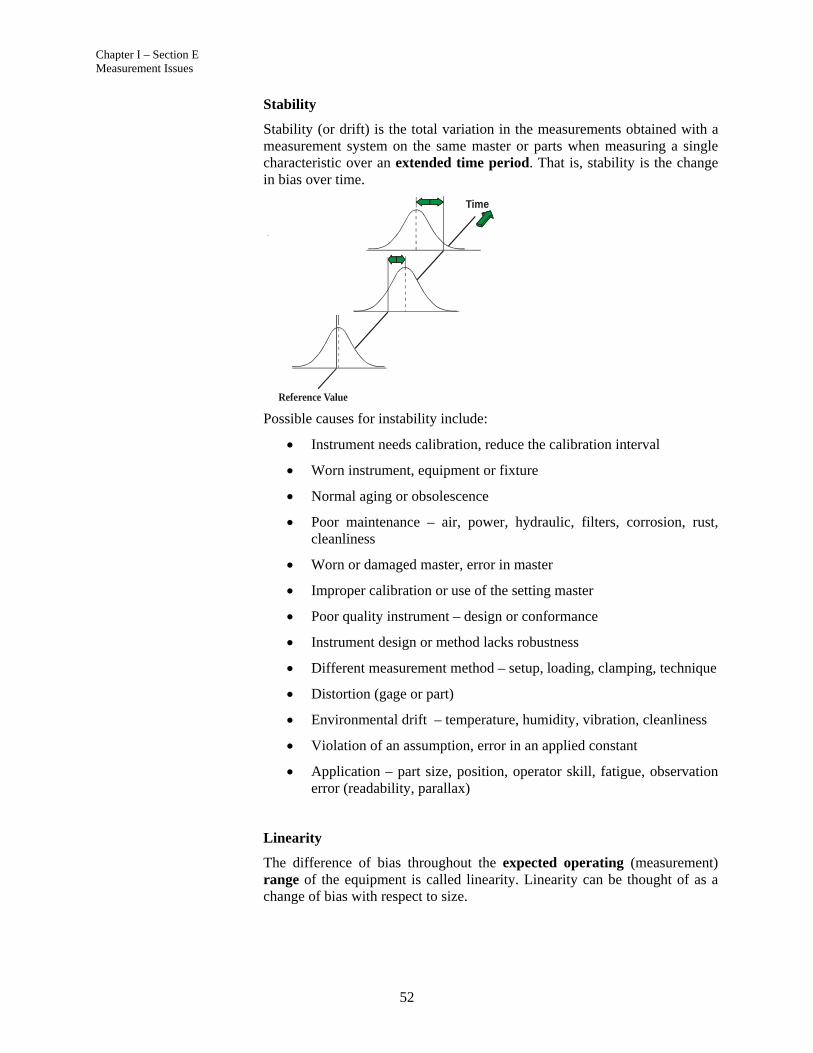
Chapter I – Section E Measurement Issues
52
Stability
Stability (or drift) is the total variation in the measurements obtained with a measurement system on the same master or parts when measuring a single characteristic over an extended time period. That is, stability is the change in bias over time.
Reference Value
Time
Possible causes for instability include:
Instrument needs calibration, reduce the calibration interval
Worn instrument, equipment or fixture
Normal aging or obsolescence
Poor maintenance – air, power, hydraulic, filters, corrosion, rust, cleanliness
Worn or damaged master, error in master
Improper calibration or use of the setting master
Poor quality instrument – design or conformance
Instrument design or method lacks robustness
Different measurement method – setup, loading, clamping, technique
Distortion (gage or part)
Environmental drift – temperature, humidity, vibration, cleanliness
Violation of an assumption, error in an applied constant
Application – part size, position, operator skill, fatigue, observation error (readability, parallax)
Linearity
The difference of bias throughout the expected operating (measurement) range of the equipment is called linearity. Linearity can be thought of as a change of bias with respect to size.

Chapter I – Section E Measurement Issues
53
Note that unacceptable linearity can come in a variety of flavors. Do not assume a constant bias.
Possible causes for linearity error include:
Instrument needs calibration, reduce the calibration interval
Worn instrument, equipment or fixture
Poor maintenance – air, power, hydraulic, filters, corrosion, rust, cleanliness
Worn or damaged master(s), error in master(s) – minimum/ maximum
BIAS BIAS
Value N Value 1

Chapter I – Section E Measurement Issues
54
Repeatability
Reference Value
Improper calibration (not covering the operating range) or use of the setting master(s)
Poor quality instrument – design or conformance
Instrument design or method lacks robustness
Wrong gage for the application
Different measurement method – setup, loading, clamping, technique
Distortion (gage or part) changes with part size
Environment – temperature, humidity, vibration, cleanliness
Violation of an assumption, error in an applied constant
Application – part size, position, operator skill, fatigue, observation error (readability, parallax)
Precision
Traditionally, precision describes the net effect of discrimination, sensitivity and repeatability over the operating range (size, range and time) of the measurement system. In some organizations precision is used interchangeably with repeatability. In fact, precision is most often used to describe the expected variation of repeated measurements over the range of measurement; that range may be size or time (i.e., “a device is as precise at the low range as high range of measurement”, or “as precise today as yesterday”). One could say precision is to repeatability what linearity is to bias (although the first is random and the other systematic errors). The ASTM defines precision in a broader sense to include the variation from different readings, gages, people, labs or conditions.
Repeatability
This is traditionally referred to as the "within appraiser" variability. Repeatability is the variation in measurements obtained with one measurement instrument when used several times by one appraiser while measuring the identical characteristic on the same part. This is the inherent variation or capability of the equipment itself. Repeatability is commonly referred to as equipment variation (EV), although this is misleading. In fact, repeatability is the common cause (random error) variation from successive trials under defined conditions of measurement. The best term for repeatability is within-system variation when the conditions of measurement are fixed and defined – fixed part, instrument, standard, method, operator, environment, and assumptions. In addition to within-equipment variation, repeatability will include all within variation (see below) from any condition in the error model.
Width Variation

Chapter I – Section E Measurement Issues
55
Possible causes for poor repeatability include:
Within-part (sample): form, position, surface finish, taper, sample consistency
Within-instrument: repair; wear, equipment or fixture failure, poor quality or maintenance
Within-standard: quality, class, wear
Within-method: variation in setup, technique, zeroing, holding, clamping
Within-appraiser: technique, position, lack of experience, manipulation skill or training, feel, fatigue
Within-environment: short-cycle fluctuations in temperature, humidity, vibration, lighting, cleanliness
Violation of an assumption – stable, proper operation
Instrument design or method lacks robustness, poor uniformity
Wrong gage for the application
Distortion (gage or part), lack of rigidity
Application – part size, position, observation error (readability, parallax)
Reproducibility
This is traditionally referred to as the "between appraisers" variability. Reproducibility is typically defined as the variation in the average of the measurements made by different appraisers using the same measuring instrument when measuring the identical characteristic on the same part. This is often true for manual instruments influenced by the skill of the operator. It is not true, however, for measurement processes (i.e., automated systems) where the operator is not a major source of variation. For this reason, reproducibility is referred to as the average variation between-systems or between-conditions of measurement.
The ASTM definition goes beyond this to potentially include not only different appraisers but also different: gages, labs and environment (temperature, humidity) as well as including repeatability in the calculation of reproducibility.
Reproducibility
Appraiser A C B
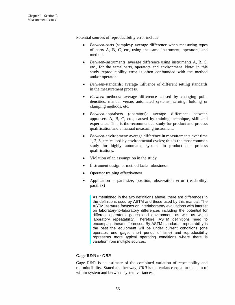
Chapter I – Section E Measurement Issues
56
Potential sources of reproducibility error include:
Between-parts (samples): average difference when measuring types of parts A, B, C, etc, using the same instrument, operators, and method.
Between-instruments: average difference using instruments A, B, C, etc., for the same parts, operators and environment. Note: in this study reproducibility error is often confounded with the method and/or operator.
Between-standards: average influence of different setting standards in the measurement process.
Between-methods: average difference caused by changing point densities, manual versus automated systems, zeroing, holding or clamping methods, etc.
Between-appraisers (operators): average difference between appraisers A, B, C, etc., caused by training, technique, skill and experience. This is the recommended study for product and process qualification and a manual measuring instrument.
Between-environment: average difference in measurements over time 1, 2, 3, etc. caused by environmental cycles; this is the most common study for highly automated systems in product and process qualifications.
Violation of an assumption in the study
Instrument design or method lacks robustness
Operator training effectiveness
Application – part size, position, observation error (readability, parallax)
As mentioned in the two definitions above, there are differences in the definitions used by ASTM and those used by this manual. The ASTM literature focuses on interlaboratory evaluations with interest on laboratory-to-laboratory differences including the potential for different operators, gages and environment as well as within laboratory repeatability. Therefore, ASTM definitions need to encompass these differences. By ASTM standards, repeatability is the best the equipment will be under current conditions (one operator, one gage, short period of time) and reproducibility represents more typical operating conditions where there is variation from multiple sources.
Gage R&R or GRR
Gage R&R is an estimate of the combined variation of repeatability and reproducibility. Stated another way, GRR is the variance equal to the sum of within-system and between-system variances.
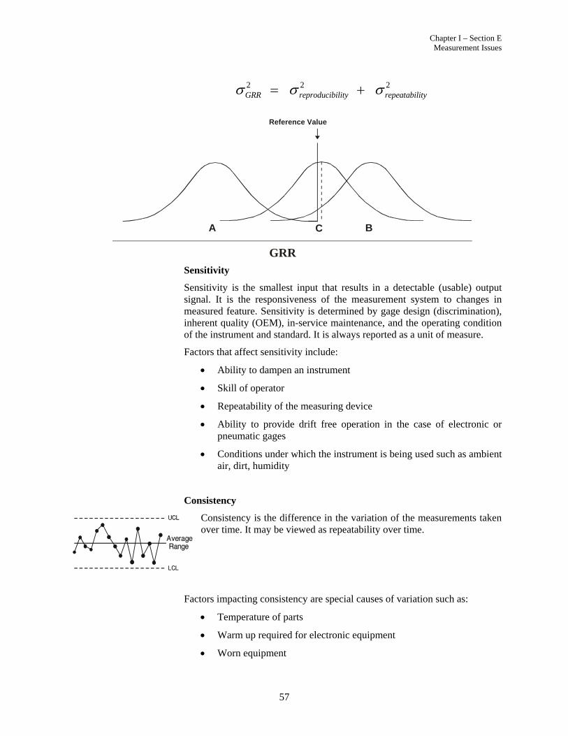
Chapter I – Section E Measurement Issues
57
2 2 2 GRR reproducibility repeatability
Sensitivity
Sensitivity is the smallest input that results in a detectable (usable) output signal. It is the responsiveness of the measurement system to changes in measured feature. Sensitivity is determined by gage design (discrimination), inherent quality (OEM), in-service maintenance, and the operating condition of the instrument and standard. It is always reported as a unit of measure.
Factors that affect sensitivity include:
Ability to dampen an instrument
Skill of operator
Repeatability of the measuring device
Ability to provide drift free operation in the case of electronic or pneumatic gages
Conditions under which the instrument is being used such as ambient air, dirt, humidity
Consistency
Consistency is the difference in the variation of the measurements taken over time. It may be viewed as repeatability over time.
Factors impacting consistency are special causes of variation such as:
Temperature of parts
Warm up required for electronic equipment
Worn equipment
Reference Value
GRR
A C B
Chapter I – Section E Measurement Issues
58
Uniformity
Uniformity is the difference in variation throughout the operating range of the gage. It may be considered to be the homogeneity (sameness) of the repeatability over size.
Factors impacting uniformity include:
Fixture allows smaller/larger sizes to position differently
Poor readability on the scale
Parallax in reading
Capability
The capability of a measurement system is an estimate of the combined variation of measurement errors (random and systematic) based on a short-term assessment. Simple capability includes the components of:
Uncorrected bias or linearity
Repeatability and reproducibility (GRR), including short-term consistency
Refer to Chapter III for typical methods and examples to quantify each component.
An estimate of measurement capability, therefore, is an expression of the expected error for defined conditions, scope and range of the measurement system (unlike measurement uncertainty, which is an expression of the expected range of error or values associated with a measurement result). The capability expression of combined variation (variance) when the measurement errors are uncorrelated (random and independent) can be quantified as:
GRRlinearitybiascapability
2
)(
22
There are two essential points to understand and correctly apply measurement capability:
First, an estimate of capability is always associated with a defined scope of measurement – conditions, range and time. For example, to say that the capability of a 25 mm micrometer is 0.1 mm is incomplete without qualifying the scope and range of measurement conditions. Again, this is why an error model to define the measurement process is so important. The scope for an estimate of measurement capability could be very specific or a general statement of operation, over a limited portion or entire measurement range. Short-term could mean: the capability over a series of measurement cycles, the time to complete the GRR evaluation, a specified period of
Measurement System Variation
Chapter I – Section E Measurement Issues
59
production, or time represented by the calibration frequency. A statement of measurement capability need only be as complete as to reasonably replicate the conditions and range of measurement. A documented Control Plan could serve this purpose.
Second, short-term consistency and uniformity (repeatability errors) over the range of measurement are included in a capability estimate. For a simple instrument, such as a 25 mm micrometer, the repeatability over the entire range of measurement using typical, skilled operators is expected to be consistent and uniform. In this example, a capability estimate may include the entire range of measurement for multiple types of features under general conditions. Longer range or more complex measurement systems (i.e., a CMM) may demonstrate measurement errors of (uncorrected) linearity, uniformity, and short-term consistency over range or size. Because these errors are correlated they cannot be combined using the simple linear formula above. When (uncorrected) linearity, uniformity or consistency varies significantly over range, the measurement planner and analyst has only two practical choices:
1) Report the maximum (worst case) capability for the entire
defined conditions, scope and range of the measurement system, or
2) Determine and report multiple capability assessments for defined portions of the measurement range (i.e., low, mid, larger range).
Performance
As with process performance, measurement system performance is the net effect of all significant and determinable sources of variation over time. Performance quantifies the long-term assessment of combined measurement errors (random and systematic). Therefore, performance includes the long-term error components of:
Capability (short-term errors)
Stability and consistency
Refer to Chapter III for typical methods and examples to quantify each component.
An estimate of measurement performance is an expression of the expected error for defined conditions, scope and range of the measurement system (unlike measurement uncertainty, which is an expression of the expected range of error or values associated with a measurement result). The performance expression of combined variation (variance) when the measurement errors are uncorrelated (random and independent) can be quantified as:
yconsistencstabilitycapabilityeperformanc
2222

Chapter I – Section E Measurement Issues
60
Again, just as short-term capability, long-term performance is always associated with a defined scope of measurement – conditions, range and time. The scope for an estimate of measurement performance could be very specific or a general statement of operation, over a limited portion or entire measurement range. Long-term could mean: the average of several capability assessments over time, the long-term average error from a measurement control chart, an assessment of calibration records or multiple linearity studies, or average error from several GRR studies over the life and range of the measurement system. A statement of measurement performance need only be as complete as to reasonably represent the conditions and range of measurement.
Long-term consistency and uniformity (repeatability errors) over the range of measurement are included in a performance estimate. The measurement analyst must be aware of potential correlation of errors so as to not overestimate the performance estimate. This depends on how the component errors were determined. When long-term (uncorrected) linearity, uniformity or consistency vary significantly over the range, the measurement planner and analyst has only two practical choices:
1) Report the maximum (worst case) performance for the entire
defined conditions, scope and range of the measurement system, or
2) Determine and report multiple performance assessments for a defined portion of the measurement range (i.e., low, mid, larger range).
Uncertainty
Measurement uncertainty is defined by VIM as a “parameter, associated with the result of a measurement, that characteristics the dispersion of the values that could reasonably be attributed to the measurand.” P
22F See
Chapter I, Section F, for more detail.
Of a measurement system’s parameters, accuracy and precision are most familiar to operating personnel since they are used in everyday life as well as technical and sales discussions. Unfortunately, these terms are also the most fuzzy as they are often thought of interchangeably. For example, if the gage is certified by an independent agency as accurate, or if the instrument is guaranteed to have high precision by the vendor, then it is incorrectly thought that all readings will fall very close to the actual values. This is not only conceptually wrong but can lead to wrong decisions about the product and process.
This ambiguity carries over to bias and repeatability (as measures of accuracy and precision). It is important to realize that:
22 Measurand is then defined by the VIM as “the particular quantity subject to measurement”.
Comments
Chapter I – Section E Measurement Issues
61
Bias and repeatability are independent of each other (See Figure I-E 6).
Controlling one of these sources of error does not guarantee the control of the other. Consequently, measurement systems control programs (traditionally referred to as Gage Control Programs) ought to quantify and track all relevant sources of variation. P
23
23 See also Chapter I, Section B.
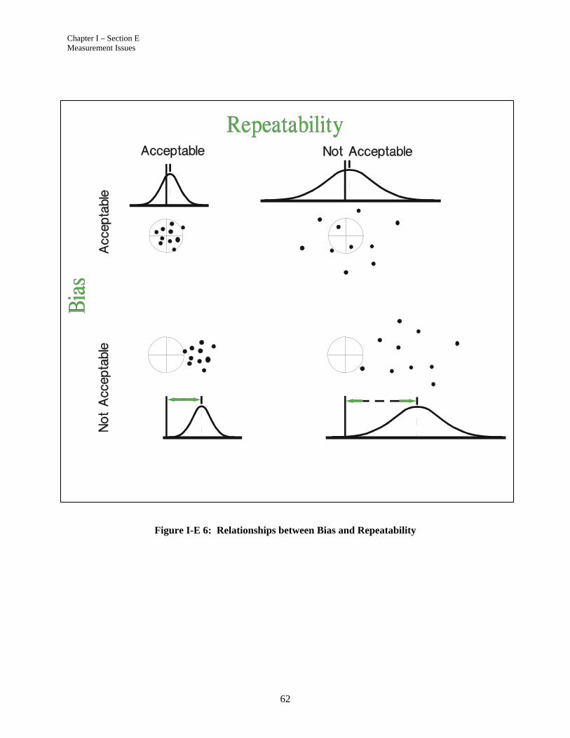
Chapter I – Section E Measurement Issues
62
Figure I-E 6: Relationships between Bias and Repeatability
Chapter I – Section F Measurement Uncertainty
63
Section F Measurement Uncertainty
Measurement Uncertainty is a term that is used internationally to describe the quality of a measurement value. While this term has traditionally been reserved for many of the high accuracy measurements performed in metrology or gage laboratories, many customer and quality system standards require that measurement uncertainty be known and consistent with required measurement capability of any inspection, measuring or test equipment.
In essence, uncertainty is the value assigned to a measurement result that describes, within a defined level of confidence, the range expected to contain the true measurement result. Measurement uncertainty is normally reported as a bilateral quantity. Uncertainty is a quantified expression of measurement reliability. A simple expression of this concept is:
True measurement = observed measurement (result) U
U is the term for “expanded uncertainty” of the measurand and measurement result. Expanded uncertainty is the combined standard error (uc), or standard deviation of the combined errors (random and systematic), in the measurement process multiplied by a coverage factor (k) that represents the area of the normal curve for a desired level of confidence. Remember, a normal distribution is often applied as a principle assumption for measurement systems. The ISO/IEC Guide to the Uncertainty in Measurement establishes the coverage factor as sufficient to report uncertainty at 95% of a normal distribution. This is often interpreted as k = 2.
ckuU
The combined standard error (uc) includes all significant components of variation in the measurement process. In most cases, methods of measurement systems analysis performed in accordance with this manual can be used as a tool to quantify many of the sources of measurement uncertainty. Often, the most significant error component can be quantified by
2performance . Other significant error sources may apply based on the
measurement application. An uncertainty statement must include an adequate scope that identifies all significant errors and allows the measurement to be replicated. Some uncertainty statements will build from long-term, others short-term, measurement system error. However, the simple expression can be quantified as:
2 2 2c performance otheru

Chapter I – Section F Measurement Uncertainty
64
It is important to remember that measurement uncertainty is simply an estimate of how much a measurement may vary at the time of measurement. It should consider all significant sources of measurement variation in the measurement process plus significant errors of calibration, master standards, method, environment and others not previously considered in the measurement process. In many cases, this estimate will use methods of MSA and GRR to quantify those significant standard errors. It is appropriate to periodically reevaluate uncertainty related to a measurement process to assure the continued accuracy of the estimate.
The major difference between uncertainty and the MSA is that the MSA focus is on understanding the measurement process, determining the amount of error in the process, and assessing the adequacy of the measurement system for product and process control. MSA promotes understanding and improvement (variation reduction). Uncertainty is the range of measurement values, defined by a confidence interval, associated with a measurement result and expected to include the true value of measurement.
Traceability is the property of a measurement or the value of a standard whereby it can be related to stated references, usually national or international standards, through an unbroken chain of comparisons all having stated uncertainties. Therefore understanding the measurement uncertainty of each link in the chain is essential. By including both the short-term and long-term sources of measurement variation that are introduced by the measurement process and the chain of traceability, the measurement system’s measurement uncertainty can be evaluated assuring that all effects of traceability are taken into account. This, in turn, may reduce measurement correlation issues.
The Guide to the Expression of Uncertainty of Measurement (GUM) is a guide to how the uncertainty of a measurement may be evaluated and expressed. While it provides the user with an understanding of the theory and sets guidelines as to how the sources of measurement uncertainty can be classified and combined, it should be considered a high level reference document, not a “how to” manual. It does provide guidance to the user in some of the more advanced topics such as, statistical independence of the sources of variation, sensitivity analysis, degrees of freedom, etc. that are critical when evaluating more complex, multi-parameter measurement systems.
Measurement Uncertainty and MSA
Measurement Traceability
ISO Guide to the Expression of Uncertainty in Measurement

Chapter I – Section G Measurement Problem Analysis
65
Section G Measurement Problem Analysis
An understanding of measurement variation and the contribution that it makes to total variation needs to be a fundamental step in basic problem solving. When variation in the measurement system exceeds all other variables, it will become necessary to analyze and resolve those issues before working on the rest of the system. In some cases the variation contribution of the measurement system is overlooked or ignored. This may cause loss of time and resources as the focus is made on the process itself, when the reported variation is actually caused by the measurement device.
In this section a review will be made on basic problem solving steps and will show how they relate to understanding the issues in a measurement system. Each company may use the problem resolution process which the customer has approved.
If the measurement system was developed using the methods in this manual, most of the initial steps will already exist. For example, a cause and effect diagram may already exist giving valuable lessons learned about the measurement process. These data ought to be collected and evaluated prior to any formal problem solving.
Identify the Issues When working with measurement systems, as with any process, it is important to clearly define the problem or issue. In the case of measurement issues, it may take the form of accuracy, variation, stability, etc. The important thing to do is try to isolate the measurement variation and its contribution, from the process variation (the decision may be to work on the process, rather than work on the measurement device). The issue statement needs to be an adequate operational definition that anyone would understand and be able to act on the issue.
Identify the Team The problem solving team, in this case, will be dependent on the complexity of the measurement system and the issue. A simple measurement system may only require a couple of people. But as the system and issue become more complex, the team may grow in size (maximum team size ought to be limited to 10 members). The team members and the function they represent need to be identified on the problem solving sheet.
Flowchart of Measurement System and Process The team would review any historical flowcharting of the measurement system and the process. This would lead to discussion of known and unknown information about the measurement and its interrelationship to the process. The flowcharting process may identify additional members to add to the team.
Step 1
Step 2
Step 3

Chapter II – Section G Measurement Problem Analysis
66
Cause and Effect Diagram The team would review any historical Cause and Effect Diagram on the Measurement System. This could, in some cases, result in the solution or a partial solution. This would also lead to a discussion on known and unknown information. The team would use subject matter knowledge to initially identify those variables with the largest contribution to the issue. Additional studies can be done to substantiate the decisions.
Plan-Do-Study-Act (PDSA) P
24 This would lead to a Plan-Do-Study-Act, which is form of scientific study. Experiments are planned, data are collected, stability is established, hypotheses are made and proven until an appropriate solution is reached.
Possible Solution and Proof of the Correction
The steps and solution are documented to record the decision. A preliminary study is performed to validate the solution. This can be done using some form of design of experiment to validate the solution. Also, additional studies can be performed over time including environmental and material variation.
Institutionalize the Change The final solution is documented in the report; then the appropriate department and functions change the process so that the problem won’t recur in the future. This may require changes in procedures, standards, and training materials. This is one of the most important steps in the process. Most issues and problems have occurred at one time or another.
24 W. Edwards Deming, The New Economics for Industry, Government, Education, The MIT Press, 1994, 2000
Step 4
Step 5
Step 6
Step 7
Chapter II General Concepts for Assessing Measurement Systems
67
CHAPTER II
General Concepts for Assessing Measurement Systems

Chapter II General Concepts for Assessing Measurement Systems
68
Chapter II – Section A Background
69
Section A Background
Two important areas need to be assessed:
1) Verify the correct variable is being measured at the proper
characteristic location. Verify fixturing and clamping if applicable. Also identify any critical environmental issues that are interdependent with the measurement. If the wrong variable is being measured, then no matter how accurate or how precise the measurement system is, it will simply consume resources without providing benefit.
2) Determine what statistical properties the measurement system needs to have in order to be acceptable. In order to make that determination, it is important to know how the data are to be used, for without that knowledge, the appropriate statistical properties cannot be determined. After the statistical properties have been determined, the measurement system must be assessed to see if it actually possesses these properties or not.
Phase 1 testing is an assessment to verify the correct variable is being measured at the proper characteristic location per measurement system design specification. (Verify fixturing and clamping if applicable) Also if there are any critical environmental issues that are interdependent with the measurement. Phase 1 could use a statistically designed experiment to evaluate the effect of the operating environment on the measurement system’s parameters (e.g., bias, linearity, repeatability, and reproducibility). Phase 1 test results can indicate that the operating environment does not contribute significantly to the overall measurement system variation. Additionally, the variation attributable to the bias and linearity of the measurement device should be small compared with the repeatability and reproducibility components.
The knowledge gained during Phase 1 testing should be used as input to the development of the measurement system maintenance program as well as the type of testing which should be used during Phase 2. Environmental issues may drive a change in location or a controlled environment for the measurement device.
For example, if there is a significant impact of repeatability and reproducibility on the total measurement system variation, a simple two-factor statistical experiment could be performed periodically as a Phase 2 test.
Phase 2 testing provides ongoing monitoring of the key sources of variation for continued confidence in the measurement system (and the data being generated) and/or a signal that the measurement system has degraded over time.
Does the measurement process satisfy the requirements over time?
Phase 1 & 2
Understand the measurement process and does it satisfy the requirements?

Chapter II – Section A Background
70
Chapter II – Section B Selecting/Developing Test Procedures
71
Section B Selecting/Developing Test Procedures
“Any technique can be useful if its limitations are understood and observed.” P
25
Many appropriate procedures are available for assessing measurement systems. The choice of which procedure to use depends on many factors, most of which need to be determined on a case-by-case basis for each measurement system to be assessed. In some cases, preliminary testing may be required to determine if a procedure is appropriate for a particular measurement system or not. Such preliminary testing ought to be an integral part of the Phase 1 testing discussed in the previous section.
General issues to consider when selecting or developing an assessment procedure include:
Should standards, such as those traceable to NIST, be used in the testing and, if so, what level of standard is appropriate? Standards are frequently essential for assessing the accuracy of a measurement system. If standards are not used, the variability of the measurement system can still be assessed, but it may not be possible to assess its accuracy with reasonable credibility. Lack of such credibility may be an issue, for instance, if attempting to resolve an apparent difference between a producer’s measurement system and a customer’s measurement system.
For the ongoing testing in Phase 2, the use of blind measurements may be considered. Blind measurements are measurements obtained in the actual measurement environment by an operator who does not know that an assessment of the measurement system is being conducted. Properly administered, tests based on blind measurements are usually not contaminated by the well-known Hawthorne effect. P
26
The cost of testing.
The time required for the testing.
Any term for which there is no commonly accepted definition should be operationally defined. Examples of such terms include accuracy, precision, repeatability, reproducibility, etc.
25 W. Edwards Deming, The Logic of Evaluation, The Handbook of Evaluation Research, Vol. 1, Elmer L.
Struening and Marcia Guttentag, Editors 26 The “Hawthorne Effect” refers to the outcomes of a series of industrial experiments performed at the
Hawthorne Works of Western Electric between November 1924 and August 1932. In the experiments, the researchers systematically modified working conditions of five assemblers and monitored the results. As the conditions improved, production rose. However, when working conditions were degraded, production continued to improve. This was thought to be the results of the workers having developed a more positive attitude toward the work solely as a result of them being part of the study, rather than as a result of the changed working conditions. See A History of the Hawthorne Experiments, by Richard Gillespie, Cambridge University Press, New York, 1991.

Chapter II – Section B Selecting/Developing Test Procedures
72
Will the measurements made by the measurement system be compared with measurements made by another system? If so, one should consider using test procedures that rely on the use of standards such as those discussed in Phase 1 above. If standards are not used, it may still be possible to determine whether or not the two measurement systems are working well together. However, if the systems are not working well together, then it may not be possible, without the use of standards, to determine which system needs improvement.
How often should Phase 2 testing be performed? This decision may be based on the statistical properties of the individual measurement system and the consequence to the facility, and the facility’s customers of a manufacturing process that, in effect, is not monitored due to a measurement system not performing properly.
In addition to these general issues, other issues that are specific to the particular measurement system being tested may also be important. Finding the specific issues that are important to a particular measurement system is one of the two objectives of the Phase 1 testing.
Chapter II – Section C Preparation for a Measurement System Study
73
Section C Preparation for a Measurement System Study
As in any study or analysis, sufficient planning and preparation ought to be done prior to conducting a measurement system study. Typical preparation prior to conducting the study is as follows:
1) The approach to be used should be planned. For instance, determine by using engineering judgment, visual observations, or a gage study, if there is an appraiser influence in calibrating or using the instrument. There are some measurement systems where the effect of reproducibility can be considered negligible; for example, when a button is pushed and a number is printed out.
2) The number of appraisers, number of sample parts, and number of repeat readings should be determined in advance. Some factors to be considered in this selection are:
(a) Criticality of dimension – critical dimensions require more parts and/or trials. The reason being the degree of confidence desired for the gage study estimations.
(b) Part configuration – bulky or heavy parts may dictate fewer samples and more trials.
(c) Customer requirements.
3) Since the purpose is to evaluate the total measurement system, the appraisers chosen should be selected from those who normally operate the instrument.
4) Selection of the sample parts is critical for proper analysis and depends entirely upon the design of the MSA study, purpose of the measurement system, and availability of part samples that represent the production process.
For Product Control situations where the measurement result and decision criteria determine, “conformance or nonconformance to the feature specification” (i.e., 100% inspection or sampling), samples (or standards) must be selected, but need not cover the entire process range. The assessment of the measurement system is based on the feature tolerance (i.e., %GRR to TOLERANCE).
For Process Control situations where the measurement result and decision criteria determine, “process stability, direction and compliance with the natural process variation” (i.e., SPC, process monitoring, capability, and process improvement), the availability of samples over the entire operating range becomes very important. An independent estimate of process variation (process capability study) is recommended when assessing the adequacy of the measurement system for process control (i.e., %GRR to process variation).
Chapter II – Section C Preparation for a Measurement System Study
74
When an independent estimate of process variation is not available, OR to determine process direction and continued suitability of the measurement system for process control, the sample parts must be selected from the process and represent the entire production operating range. The variation in sample parts (PV) selected for MSA study is used to calculate the Total Variation (TV) of the study. The TV index (i.e., %GRR to TV) is an indicator of process direction and continued suitability of the measurement system for process control. If the sample parts DO NOT represent the production process, TV must be ignored in the assessment. Ignoring TV does not affect assessments using tolerance (product control) or an independent estimate of process variation (process control).
Samples can be selected by taking one sample per day for several days. Again, this is necessary because the parts will be treated in the analysis as if they represent the range of production variation in the process. Since each part will be measured several times, each part must be numbered for identification.
5) The instrument should have a discrimination that allows at least one-tenth of the expected process variation of the characteristic to be read directly. For example, if the characteristic’s variation is 0.001, the equipment should be able to “read” a change of 0.0001.
6) Assure that the measuring method (i.e., appraiser and instrument) is measuring the dimension of the characteristic and is following the defined measurement procedure.
The manner in which a study is conducted is very important. All analyses presented in this manual assume statistical independence P
27F of the individual
readings. To minimize the likelihood of misleading results, the following steps need to be taken:
1) The measurements should be made in a random order P
28F to
ensure that any drift or changes that could occur will be spread randomly throughout the study. The appraisers should be unaware of which numbered part is being checked in order to avoid any possible knowledge bias. However, the person conducting the study should know which numbered part is being checked and record the data accordingly, that is Appraiser A, Part 1, first trial; Appraiser B, Part 4, second trial, etc.
2) In reading the equipment, measurement values should be recorded to the practical limit of the instrument discrimination. Mechanical devices must be read and recorded to the smallest unit of scale discrimination. For electronic readouts, the measurement plan must establish a common policy for recording the right-most significant digit of display. Analog devices should
27 There is no correlation between readings. 28 See Chapter III, Section B, “Randomization and Statistical Independence”

Chapter II – Section C Preparation for a Measurement System Study
75
be recorded to one-half the smallest graduation or limit of sensitivity and resolution. For analog devices, if the smallest scale graduation is 0.0001”, then the measurement results should be recorded to 0.00005”.
3) The study should be managed and observed by a person who understands the importance of conducting a reliable study.
When developing Phase 1 or Phase 2 test programs there are several factors that need to be considered:
What effect does the appraiser have on the measurement process? If possible, the appraisers who normally use the measurement device should be included in the study.
Each appraiser should use the procedure – including all steps – they normally use to obtain readings. The effect of any differences between methods the appraisers use will be reflected in the Reproducibility of the measurement system.
Is appraiser calibration of the measurement equipment likely to be a significant cause of variation? If so, the appraisers should recalibrate the equipment before each group of readings.
How many sample parts and repeated readings are required? The number of parts required will depend upon the significance of the characteristic being measured and upon the level of confidence required in the estimate of measurement system variation.
Although the number of appraisers, trials and parts may be varied when using the recommended practices discussed in this manual, the number of appraisers, trials and parts should remain constant between Phase 1 and Phase 2 test programs or between sequential Phase 2 tests for common measurement systems. Maintaining commonality between test programs and sequential tests will improve comparisons between the various test results.

Chapter II – Section C Preparation for a Measurement System Study
76

Chapter II – Section D Analysis of the Results
77
Section D Analysis of the Results
The results should be evaluated to determine if the measurement device is acceptable for its intended application. A measurement system should be stable before any additional analysis is valid.
Acceptability Criteria – Gage Assembly and Fixture Error
An improperly designed fixture or poorly assembled gage will increase measurement error. This is normally found when the measurements indicate or display process instability or out-of-control conditions. This may be due to excessive gage variation or poor repeatability and poor GRR values.
In general, the first thing to do when an apparent measurement issue exists, is to review the assembly and setup instructions to make sure the gage was properly assembled, (NOTE: this will not be in the instructions) and, for example, the clamps/probes are positioned properly and have the right load. Also, for automated measurement, verify the program follows required or expected protocol.
If problems are found in any of these areas, reset or repair the gage and fixtures, then rerun the measurement evaluation.
Acceptability Criteria – Location Error
Location error is normally defined by analyzing bias and linearity.
In general, the bias or linearity error of a measurement system is unacceptable if it is significantly different from zero or exceeds the maximum permissible error established by the gage calibration procedure. In such cases, the measurement system should be recalibrated or an offset correction applied to minimize this error.
Acceptability Criteria – Width Error
The criteria as to whether a measurement system’s variability is satisfactory are dependent upon the percentage of the manufacturing production process variability or the part tolerance that is consumed by measurement system variation. The final acceptance criteria for specific measurement systems depend on the measurement system’s environment and purpose and should be agreed to by the customer. (See Chapter I Section B- “The Effects of Measurement System Variability”)
When beginning to evaluate an organization’s measurement systems, it can be useful to set priorities on which measurement systems to initially focus. Since the final (total) variation is based on a combination of the process and measurement variation,
( Total Process MSA 2 2 ), when SPC is being applied for
process control or collecting process data, and the control chart indicates that the process is stable and the total variation is acceptable, the measurement system can be considered
Width Error
Location Error
Assembly or Fixture Error

Chapter II – Section D Analysis of the Results
78
acceptable for this use and does not require separate re-evaluation P
29F. If an out-of-control condition or nonconformance is
found in this situation, the first thing that should be done is to evaluate the measurement system.
For measurement systems whose purpose is to analyze a process, a general guidelines for measurement system acceptability is as follows:
GRR Decision Comments
Under 10 percent
Generally considered to be an acceptable measurement system.
Recommended, especially useful when trying to sort or classify parts or when tightened process control is required.
10 percent to 30 percent
May be acceptable for some applications
Decision should be based upon, for example, importance of application measurement, cost of measurement device, cost of rework or repair.
Should be approved by the customer.
Over 30 percent
Considered to be unacceptable Every effort should be made to improve the measurement system.
This condition may be addressed by the use of an appropriate measurement strategy; for example, using the average result of several readings of the same part characteristic in order to reduce final measurement variation.
Table II-D 1: GRR Criteria
Additional Width Error Metric
Another statistic of the measurement system variability is the number of distinct categories (ndc) P
30F. This statistic indicates the number of categories
into which the measurement process can be divided. This value should be greater than or equal to 5.
Caution: The use of the GRR guidelines as threshold criteria alone is NOT an acceptable practice for determining the acceptability of a measurement system.
29 If the total process is in statistical control for both the mean and variation charts and the total variation is
acceptable then it can be assumed either (1) both the actual process and measurement variability are acceptable or (2) the measurement variation is not acceptable with respect to the process variation (which is extremely small) but both are in statistical control. In either case the process is producing acceptable product. In case (2) the existence of a nonconformance or out of control condition could be a false alarm (i.e., the product is acceptable but the evaluation says it is not) which would cause an evaluation of both the measurement system and process.
30 See Chapter I, Section E, “Measurement Issues”.

Chapter II – Section D Analysis of the Results
79
Applying the guidelines as the thresholds assumes that the calculated statistics are deterministic estimates of the measurement system’s variability (which they are not). Specifying the guidelines as the threshold criteria can drive the wrong behavior. For example, the supplier may be creative in achieving a low GRR by eliminating real life sources of variation (e.g., part to gage interaction) or manipulating the measurement study (e.g., producing parts outside the expected process variation).
Comments on the Application and Gage Acceptability
When looking at GRR and measurement variation it is important to look at each application individually, to see what is required and how the measurement is going to be used. For example: the required precision of temperature measurement may be different for dissimilar applications. A room thermostat can regulate the temperature for human comfort and is economically priced, but may have a GRR upwards to 30%. It is acceptable for this application. But in a laboratory, where small variations in temperature can impact test results, a more sophisticated temperature measurement and control is required. This thermostat will be more expensive and is required to have less variability (i.e., to have a lower GRR).
The final acceptance of a measurement system should not come down to a single set of indices. The long-term performance of the measurement system should also be reviewed, for example, using graphical analysis over time.

Chapter II – Section D Analysis of the Results
80

Chapter III Recommended Practices for Replicable Measurement Systems
81
CHAPTER III
Recommended Practices for Replicable Measurement Systems

Chapter III – Section A Example Test Procedures
82
Chapter III – Section A Example Test Procedures
83
Section A Example Test Procedures
Examples of specific test procedures are presented in this chapter. The procedures are simple to use and can be readily applied in a production environment. As discussed previously, the test procedure which should be used to understand a measurement system and to quantify its variability depends on the sources of variation which may affect the measurement system. In many situations the major sources of variation are due to the instrument (gage/equipment), person (appraiser), and method (measurement procedure). The test procedures in this chapter are sufficient for this type of measurement system analysis.
The procedures are appropriate to use when:
Only two factors or conditions of measurement (i.e., appraisers and parts) plus measurement system repeatability are being studied
The effect of the variability within each part is negligible There is no statistical interaction between appraisers and parts The parts do not change functionally or dimensionally during the
study, i.e., are replicable
A statistical design of experiment can be conducted and/or subject matter knowledge used to determine if these procedures are appropriate for any specific measurement system.

Chapter III – Section A Example Test Procedures
84
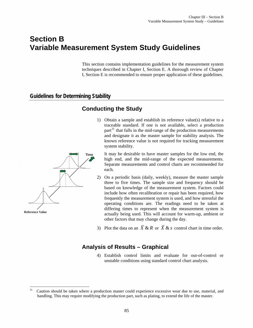
Chapter III – Section B Variable Measurement System Study – Guidelines
85
Section B Variable Measurement System Study Guidelines
This section contains implementation guidelines for the measurement system techniques described in Chapter I, Section E. A thorough review of Chapter I, Section E is recommended to ensure proper application of these guidelines.
Guidelines for Determining Stability
Conducting the Study
1) Obtain a sample and establish its reference value(s) relative to a traceable standard. If one is not available, select a production part P
31F that falls in the mid-range of the production measurements
and designate it as the master sample for stability analysis. The known reference value is not required for tracking measurement system stability.
It may be desirable to have master samples for the low end, the high end, and the mid-range of the expected measurements. Separate measurements and control charts are recommended for each.
2) On a periodic basis (daily, weekly), measure the master sample three to five times. The sample size and frequency should be based on knowledge of the measurement system. Factors could include how often recalibration or repair has been required, how frequently the measurement system is used, and how stressful the operating conditions are. The readings need to be taken at differing times to represent when the measurement system is actually being used. This will account for warm-up, ambient or other factors that may change during the day.
3) Plot the data on an &X R or &X s control chart in time order.
Analysis of Results – Graphical 4) Establish control limits and evaluate for out-of-control or
unstable conditions using standard control chart analysis.
31 Caution should be taken where a production master could experience excessive wear due to use, material, and
handling. This may require modifying the production part, such as plating, to extend the life of the master.
Reference Value
Time
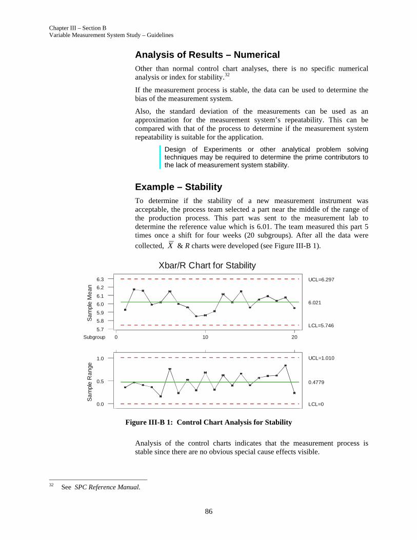
Chapter III – Section B Variable Measurement System Study – Guidelines
86
Analysis of Results – Numerical Other than normal control chart analyses, there is no specific numerical analysis or index for stability. P
32F
If the measurement process is stable, the data can be used to determine the bias of the measurement system.
Also, the standard deviation of the measurements can be used as an approximation for the measurement system’s repeatability. This can be compared with that of the process to determine if the measurement system repeatability is suitable for the application.
Design of Experiments or other analytical problem solving techniques may be required to determine the prime contributors to the lack of measurement system stability.
Example – Stability To determine if the stability of a new measurement instrument was acceptable, the process team selected a part near the middle of the range of the production process. This part was sent to the measurement lab to determine the reference value which is 6.01. The team measured this part 5 times once a shift for four weeks (20 subgroups). After all the data were
collected, X & R charts were developed (see Figure III-B 1).
Figure III-B 1: Control Chart Analysis for Stability
Analysis of the control charts indicates that the measurement process is stable since there are no obvious special cause effects visible.
32 See SPC Reference Manual.
0Subgroup 10 20
5.7
5.8
5.9
6.0
6.1
6.2
6.3
Sa
mpl
eM
ea
n
6.021
UCL=6.297
LCL=5.746
0.0
0.5
1.0
Sa
mpl
eR
ang
e
0.4779
UCL=1.010
LCL=0
Xbar/R Chart for Stability

Chapter III – Section B Variable Measurement System Study – Guidelines
87
Guidelines for Determining Bias P
33F – Independent Sample Method
Conducting the Study The independent sample method for determining whether the bias is acceptable uses the Test of Hypothesis:
0
1
0
0
H bias
H bias
The calculated average bias is evaluated to determine if the bias could be due to random (sampling) variation.
In general, the bias or linearity error of a measurement system is acceptable if it is not statistically significantly different from zero when compared to the repeatability. Consequently, the repeatability must be acceptable when compared to the process variation in order for this analysis to be useful.
1) Obtain a sample and establish its reference value relative to a traceable standard. If one is not available, select a production part that falls in the mid-range of the production measurements and designate it as the master sample for bias analysis. Measure the part n 10 times in the gage or tool room, and compute the average of the n readings. Use this average as the “reference value.”
It may be desirable to have master samples for the low end of the expected measurements, the high end, and the mid-range. If this is done, analyze the data using a linearity study.
2) Have a single appraiser measure the sample n 10 times in the
normal manner.
Analysis of Results – Graphical
3) Determine the bias of each reading:
i ibias x reference value
4) Plot the bias data as a histogram relative to the reference value. Review the histogram, using subject matter knowledge, to determine if any special causes or anomalies are present. If not, continue with the analysis. Special caution ought to be exercised for any interpretation or analysis when n < 30.
33 See Chapter I, Section E, for an operational definition and discussion of potential causes.
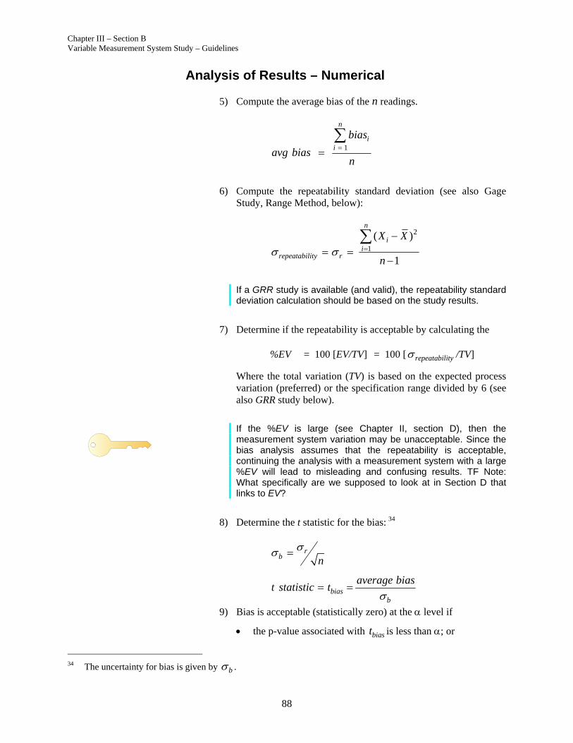
Chapter III – Section B Variable Measurement System Study – Guidelines
88
Analysis of Results – Numerical
5) Compute the average bias of the n readings.
1
n
ii
bias
avg biasn
6) Compute the repeatability standard deviation (see also Gage
Study, Range Method, below):
2
1
( )
1
n
ii
repeatability r
X X
n
If a GRR study is available (and valid), the repeatability standard deviation calculation should be based on the study results.
7) Determine if the repeatability is acceptable by calculating the
%EV = 100 [EV/TV] = 100 [ repeatability /TV]
Where the total variation (TV) is based on the expected process variation (preferred) or the specification range divided by 6 (see also GRR study below).
If the %EV is large (see Chapter II, section D), then the measurement system variation may be unacceptable. Since the bias analysis assumes that the repeatability is acceptable, continuing the analysis with a measurement system with a large %EV will lead to misleading and confusing results. TF Note: What specifically are we supposed to look at in Section D that links to EV?
8) Determine the t statistic for the bias: F
34
rb n
biasb
average biast statistic t
9) Bias is acceptable (statistically zero) at the level if
the p-value associated with biast is less than ; or
34 The uncertainty for bias is given by b .
Chapter III – Section B Variable Measurement System Study – Guidelines
89
zero falls within the 1- confidence bounds based on the bias value:
b b, 1 , 12 2σ σBias t zero Bias t
where = n – 1 and
,1 2t
is found using the standard t tables.
The level which is used depends on the level of sensitivity which is needed to evaluate/control the process and is associated with the loss function (sensitivity curve) of the product/process. Customer agreement should be obtained if an level other than the default value of .05 (95% confidence) is used.
Example – Bias A manufacturing engineer was evaluating a new measurement system for monitoring a process. An analysis of the measurement equipment indicated that there should be no linearity concerns, so the engineer had only the bias of the measurement system evaluated. A single part was chosen within the operating range of the measurement system based upon documented process variation. The part was measured by layout inspection to determine its reference value. The part was then measured fifteen times by the lead operator.
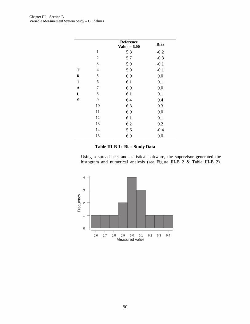
Chapter III – Section B Variable Measurement System Study – Guidelines
90
Reference
Value = 6.00 Bias
1 5.8 -0.2 2 5.7 -0.3 3 5.9 -0.1
T 4 5.9 -0.1 R 5 6.0 0.0 I 6 6.1 0.1 A 7 6.0 0.0 L 8 6.1 0.1 S 9 6.4 0.4 10 6.3 0.3 11 6.0 0.0 12 6.1 0.1 13 6.2 0.2 14 5.6 -0.4 15 6.0 0.0
Table III-B 1: Bias Study Data
Using a spreadsheet and statistical software, the supervisor generated the histogram and numerical analysis (see Figure III-B 2 & Table III-B 2).
5.6 5.7 5.8 5.9 6.0 6.1 6.2 6.3 6.4
0
1
2
3
4
Fre
qu
ency
Measured value
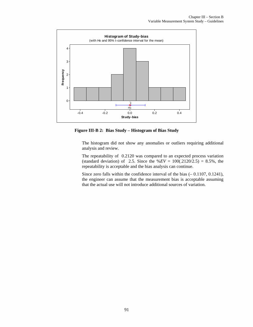
Chapter III – Section B Variable Measurement System Study – Guidelines
91
0.40.20.0-0.2-0.4
4
3
2
1
0X_
Ho
Study-bias
Freq
uenc
y
Histogram of Study-bias(with Ho and 95% t-confidence interval for the mean)
Figure III-B 2: Bias Study – Histogram of Bias Study
The histogram did not show any anomalies or outliers requiring additional analysis and review.
The repeatability of 0.2120 was compared to an expected process variation (standard deviation) of 2.5. Since the %EV = 100(.2120/2.5) = 8.5%, the repeatability is acceptable and the bias analysis can continue.
Since zero falls within the confidence interval of the bias (– 0.1107, 0.1241), the engineer can assume that the measurement bias is acceptable assuming that the actual use will not introduce additional sources of variation.

Chapter III – Section B Variable Measurement System Study – Guidelines
92
Table III-B 2: Bias Study – Analysis of Bias Study P
35
Guidelines for Determining Bias – Control Chart Method
Conducting the Study
If an X & R chart is used to measure stability, the data can also be used to evaluate bias. The control chart analysis should indicate that the measurement system is stable before the bias is evaluated.
1) Obtain a sample and establish its reference value relative to a
traceable standard. If one is not available, select a production part that falls in the mid-range of the production measurements and designate it as the master sample for bias analysis. Measure the part n 10 times in the gage or tool room, and compute the average of the n readings. Use this average as the “reference value.”
2) Conduct the stability study with g (subgroups) ≥ 20 subgroups of size m.
35 Even though data is given with one digit after the decimal point, the results are shown as provided by a typical
statistical program using double precision; i.e., with multiple decimal digits.
Measured Value 0.12 14
Significant t value
(2-tailed)
Average
Bias
2.14479 -0.1107
df
t
statistic
0.1241 .0067
95% Confidence Interval of the Bias
Lower Upper
Reference Value = 6.00, =.05
Measured Value
15 6.0067
Standard Deviation,
Standard Error of Mean,
0.2120 0.0547
n brAverage
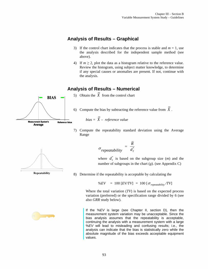
Chapter III – Section B Variable Measurement System Study – Guidelines
93
Analysis of Results – Graphical
3) If the control chart indicates that the process is stable and m = 1, use the analysis described for the independent sample method (see above).
4) If m ≥ 2, plot the data as a histogram relative to the reference value. Review the histogram, using subject matter knowledge, to determine if any special causes or anomalies are present. If not, continue with the analysis.
Analysis of Results – Numerical 5) Obtain the X from the control chart
6) Compute the bias by subtracting the reference value from X .
bias = X – reference value
7) Compute the repeatability standard deviation using the Average
Range
*2
R
drepeatability
where *2d is based on the subgroup size (m) and the
number of subgroups in the chart (g). (see Appendix C)
8) Determine if the repeatability is acceptable by calculating the
%EV = 100 [EV/TV] = 100 [ repeatability /TV]
Where the total variation (TV) is based on the expected process variation (preferred) or the specification range divided by 6 (see also GRR study below).
If the %EV is large (see Chapter II, section D), then the measurement system variation may be unacceptable. Since the bias analysis assumes that the repeatability is acceptable, continuing the analysis with a measurement system with a large %EV will lead to misleading and confusing results; i.e., the analysis can indicate that the bias is statistically zero while the absolute magnitude of the bias exceeds acceptable equipment values.
Chapter III – Section B Variable Measurement System Study – Guidelines
94
9) Determine the t statistic for the bias: P
36
rb gm
biasb
biast statistic t
10) Bias is acceptable (statistically zero) at the level if zero falls within the 1- confidence bounds around the bias value:
b b, 1 , 12 2σ σBias t zero Bias t
where is found in Appendix C
and,1 2
t is found using the standard t tables.
The level which is used depends on the level of sensitivity which is needed to evaluate/control the process and is associated with the loss function (sensitivity curve) of the product/process. Customer agreement should be obtained if an level other than the default value of .05 (95% confidence) is used.
Example – Bias Referencing Figure III-B 1, the stability study was performed on a part which had a reference value of 6.01. The overall average of all the samples (20 subgroups of size 5 for n=100 samples) was 6.021. The calculated bias is therefore 0.011.
Using a spreadsheet and statistical software, the supervisor generated the numerical analysis (Table III-B 3).
Since zero falls within the confidence interval of the bias (-0.0299, 0.0519), the process team can assume that the measurement bias is acceptable assuming that the actual use will not introduce additional sources of variation.
36 The uncertainty for bias is given by b .
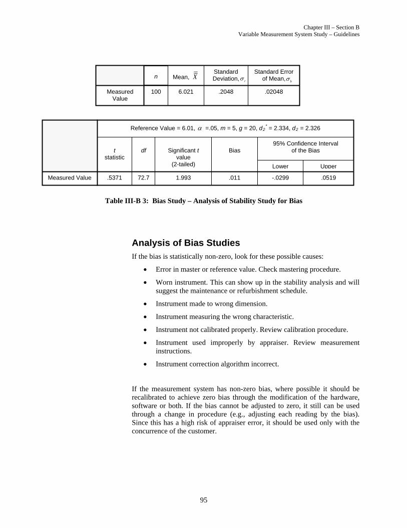
Chapter III – Section B Variable Measurement System Study – Guidelines
95
Table III-B 3: Bias Study – Analysis of Stability Study for Bias
Analysis of Bias Studies If the bias is statistically non-zero, look for these possible causes:
Error in master or reference value. Check mastering procedure.
Worn instrument. This can show up in the stability analysis and will suggest the maintenance or refurbishment schedule.
Instrument made to wrong dimension.
Instrument measuring the wrong characteristic.
Instrument not calibrated properly. Review calibration procedure.
Instrument used improperly by appraiser. Review measurement instructions.
Instrument correction algorithm incorrect.
If the measurement system has non-zero bias, where possible it should be recalibrated to achieve zero bias through the modification of the hardware, software or both. If the bias cannot be adjusted to zero, it still can be used through a change in procedure (e.g., adjusting each reading by the bias). Since this has a high risk of appraiser error, it should be used only with the concurrence of the customer.
Measured Value .5371 72.7
Significant t
value (2-tailed)
Bias
1.993 -.0299
df
t
statistic
.0519 .011
95% Confidence Interval of the Bias
Lower Upper
Reference Value = 6.01, =.05, m = 5, g = 20, d2 P
* = 2.334, d2 = 2.326
Measured Value
100 6.021
Standard Deviation,
Standard Error of Mean,
.2048 .02048
n brMean, X

Chapter III – Section B Variable Measurement System Study – Guidelines
96
Guidelines for Determining Linearity P
37
Conducting the Study
Linearity can be evaluated using the following guidelines:
1) Select g 5 parts whose measurements, due to process variation, cover the operating range of the gage.
2) Have each part measured by layout inspection to determine its reference value and to confirm that the operating range of the subject gage is encompassed.
3) Have each part measured m 10 times on the subject gage by one of the operators who normally use the gage.
Select the parts at random to minimize appraiser “recall” bias in the measurements.
Analysis of Results – Graphical 4) Calculate the part bias for each measurement and the bias average for
each part.
, ,i j i j ibias x reference value
,1
m
i jj
i
bias
biasm
5) Plot the individual biases and the bias averages with respect to the reference values on a linear graph. (see Figure III-B 3.)
6) Calculate and plot the best fit line and the confidence band of the line using the following equations.
For the best fit line, use: i iy a x b
where
ix = reference value
iy = bias average
and
37 See Chapter I, Section E, for an operational definition and discussion of potential causes.
Value 1 Value N

Chapter III – Section B Variable Measurement System Study – Guidelines
97
22
1
1
xy x ygm
a slopex x
gm
b y ax intercept
For a given x0 , the level confidence bands P
38F are:
where 2
2i i i iy b y a x y
sgm
lower:
2
02
12
0 2,1 21
igm
x x
x xb a x t s
gm
upper:
2
02
12
0 2,1 21
igm
x x
x xb a x t s
gm
7) The standard deviation of the variability of repeatability.
repeatability
s
Determine if the repeatability is acceptable by calculating the
%EV = 100 [EV/TV] = 100 [ repeatability /TV]
Where the total variation (TV) is based on the expected process variation (preferred) or the specification range divided by 6 (see also GRR study below).
If the %EV is large (see Chapter II, section D), then the measurement system variation may be unacceptable. Since the bias analysis assumes that the repeatability is acceptable, continuing the analysis with a measurement system with a large %EV will lead to misleading and confusing results.
8) Plot the “bias = 0” line and review the graph for indications of special causes and the acceptability of the linearity. (see example Figure III-B 3.)
38 See the note on selecting the level in the “Guidelines for Determining Bias” area in Chapter III, Section B.

Chapter III – Section B Variable Measurement System Study – Guidelines
98
For the measurement system linearity to be acceptable, the “bias = 0” line must lie entirely within the confidence bands of the fitted line.
Analysis of Results – Numerical 9) If the graphical analysis indicates that the measurement system
linearity is acceptable then the following hypothesis should be true:
H0: a = 0 slope = 0
do not reject if
2, 1 2
2
gm
j
at t
s
x x
If the above hypothesis is true then the measurement system has the same bias for all reference values. For the linearity to be acceptable this bias must be zero.
Ho: b = 0 intercept (bias) = 0
do not reject if
2, 1 22
2
1gm
i
bt t
xs
gm x x
Example – Linearity A plant supervisor was introducing a new measurement system to the process. As part of the PPAP P
39F the linearity of the measurement system
needed to be evaluated. Five parts were chosen throughout the operating range of the measurement system based upon documented process variation. Each part was measured by layout inspection to determine its reference value. Each part was then measured twelve times by the lead operator. The parts were selected at random during the study.
39 Production Parts Approval Process manual, 4th Edition, 2006

Chapter III – Section B Variable Measurement System Study – Guidelines
99
Part 1 2 3 4 5
Reference
Value
2.00
4.00
6.00
8.00
10.00 1 2.70 5.10 5.80 7.60 9.10 2 2.50 3.90 5.70 7.70 9.30 3 2.40 4.20 5.90 7.80 9.50
T 4 2.50 5.00 5.90 7.70 9.30 R 5 2.70 3.80 6.00 7.80 9.40 I 6 2.30 3.90 6.10 7.80 9.50 A 7 2.50 3.90 6.00 7.80 9.50 L 8 2.50 3.90 6.10 7.70 9.50 S 9 2.40 3.90 6.40 7.80 9.60 10 2.40 4.00 6.30 7.50 9.20 11 2.60 4.10 6.00 7.60 9.30 12 2.40 3.80 6.10 7.70 9.40
Table III-B 4: Linearity Study Data
Using a spreadsheet and statistical software, the supervisor generated the linearity plot (Figure III-B 3).
Part 1 2 3 4 5 Reference
Value
2.00
4.00
6.00
8.00
10.00 1 0.7 1.1 -0.2 -0.4 -0.9 2 0.5 -0.1 -0.3 -0.3 -0.7
3 0.4 0.2 -0.1 -0.2 -0.5
B 4 0.5 1.0 -0.1 -0.3 -0.7
I 5 0.7 -0.2 0.0 -0.2 -0.6
A 6 0.3 -0.1 0.1 -0.2 -0.5
S 7 0.5 -0.1 0.0 -0.2 -0.5
8 0.5 -0.1 0.1 -0.3 -0.5
9 0.4 -0.1 0.4 -0.2 -0.4
10 0.4 0.0 0.3 -0.5 -0.8
11 0.6 0.1 0.0 -0.4 -0.7
12 0.4 -0.2 0.1 -0.3 -0.6
BIAS Avg. 0.491667 0.125 0.025 -0.29167 -0.61667
Table III-B 5: Linearity Study – Intermediate Results

Chapter III – Section B Variable Measurement System Study – Guidelines
100
Figure III-B 3: Linearity Study – Graphical Analysis
The graphical analysis indicates that special causes may be influencing the measurements system. The data for reference value 4 appear to be bimodal.
Even if the data for reference value 4 were not considered, the graphical analysis clearly shows that this measurement system has a linearity problem. The R2 value indicates that a linear model may not be an appropriate model for these data. P
40F Even if the linear model is accepted, the “bias = 0” line
intersects the confidence bounds rather than being contained by them.
At this point, the supervisor ought to begin problem analysis and resolution on the measurement system, since the numerical analysis will not provide any additional insights. However, wanting to make sure no paperwork is left unmarked, the supervisor calculates the t-statistic for the slope and intercept:
12.043at
10.158bt
Taking the default = .05 and going to the t-tables with (gm – 2) = 58 degrees of freedom and a proportion of .975, the supervisor comes up with the critical value of:
40 See standard statistical texts on analysis of the appropriateness of using a linear model to describe the
relationship between two variables.
109876 5 4 3 2
1
0
-1
R-Sq = 71.4 %
Y = 0.736667 - 0.131667X
95% CI
Regression
Linearity Example
Bias Average
Reference Values
Bia
s
Bias = 0

Chapter III – Section B Variable Measurement System Study – Guidelines
101
58, .975 2.00172t
Since 58, .975 at t , the result obtained from the graphical analysis is
reinforced by the numerical analysis – there is a linearity problem with this measurement system.
In this case, it does not matter what relation bt has to 58, .975t since there is a
linearity problem. Possible causes for linearity problems can be found in Chapter I, Section E, “Location Variation.”
If the measurement system has a linearity problem, it needs to be recalibrated to achieve zero bias through the modification of the hardware, software or both.
If the bias cannot be adjusted to zero bias throughout the measurement system range, it still can be used for product/process control but not analysis as long as the measurement system remains stable.
Since this has a high risk of appraiser error, it should be used only with the concurrence of the customer.
Guidelines for Determining Repeatability and Reproducibility P
41
The Variable Gage Study can be performed using a number of differing techniques. Three acceptable methods will be discussed in detail in this section. These are:
Range method
Average and Range method (including the Control Chart method)
ANOVA method
Except for the Range method, the study data design is very similar for each of these methods. The ANOVA method is preferred because it measures the operator to part interaction gauge error, whereas the Range and the Average and Range methods does not include this variation. As presented, all methods ignore within-part variation (such as roundness, diametric taper, flatness, etc., as discussed in Chapter IV, Section D) in their analyses.
The ANOVA approach can identify appraiser-part interaction but it can also evaluate other sources of variation which is the reason why it was included. Historically, the assumption is made that the interaction is zero, in which case the results of both approaches are equivalent. With that said, the ANOVA approach is preferred because of its flexibility if the user has access to a appropriate computer program. If not, the X bar and R approach is appropriate and can be done manually or via a computer program.
41 See Chapter I, Section E, for an operational definition and discussion of potential causes.

Chapter III – Section B Variable Measurement System Study – Guidelines
102
However, the total measurement system includes not only the gage itself and its related bias, repeatability, etc., but also could include the variation of the parts being checked. The determination of how to handle within-part variation needs to be based on a rational understanding of the intended use of the part and the purpose of the measurement.
Finally, all of the techniques in this section are subject to the prerequisite of statistical stability.
Although reproducibility is usually interpreted as appraiser variation, there are situations when this variation is due to other sources of variation. For example, with some in-process measurement systems there are no human appraisers. If all the parts are handled, fixtured and measured by the same equipment, then reproducibility is zero; i.e., only a repeatability study is needed. If, however, multiple fixtures are used, then the reproducibility is the between-fixture variation.
Range Method
The Range method is a modified variable gage study which will provide a quick approximation of measurement variability. This method will provide only the overall picture of the measurement system. It does not decompose the variability into repeatability and reproducibility. It is typically used as a quick check to verify that the GRR has not changed.
This approach has the potential to detect an unacceptable measurement system P
42F 80% of the time with a sample size of 5
and 90% of the time with a sample size of 10.
The Range method typically uses two appraisers and five parts for the study. In this study, both appraisers measure each part once. The range for each part is the absolute difference between the measurement obtained by appraiser A and the measurement obtained by appraiser B. The sum of the ranges is
found and the average range ( R ) is calculated. The total measurement
variability is found by multiplying the average range by *2
1d
where *2d is
found in Appendix C, with m = 2 and g = number of parts.
Parts Appraiser A Appraiser B Range (A, B)
1 0.85 0.80 0.05
2 0.75 0.70 0.05
3 1.00 0.95 0.05
4 0.45 0.55 0.10
5 0.50 0.60 0.10
42 i.e., %GRR > 30%
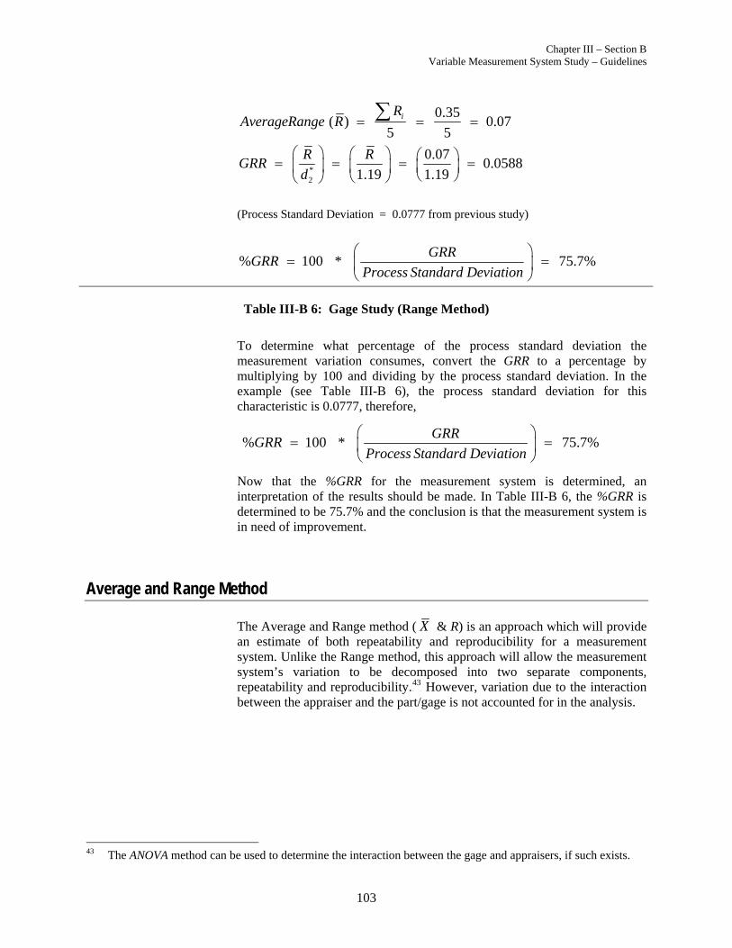
Chapter III – Section B Variable Measurement System Study – Guidelines
103
0.35( ) 0.07
5 5iR
AverageRange R
*2
0.07 0.0588
1.19 1.19
R RGRR
d
(Process Standard Deviation = 0.0777 from previous study)
% 100 * 75.7%GRR
GRR Process Standard Deviation
Table III-B 6: Gage Study (Range Method)
To determine what percentage of the process standard deviation the measurement variation consumes, convert the GRR to a percentage by multiplying by 100 and dividing by the process standard deviation. In the example (see Table III-B 6), the process standard deviation for this characteristic is 0.0777, therefore,
% 100 * 75.7%GRR
GRR Process Standard Deviation
Now that the %GRR for the measurement system is determined, an interpretation of the results should be made. In Table III-B 6, the %GRR is determined to be 75.7% and the conclusion is that the measurement system is in need of improvement.
Average and Range Method
The Average and Range method ( X & R) is an approach which will provide an estimate of both repeatability and reproducibility for a measurement system. Unlike the Range method, this approach will allow the measurement system’s variation to be decomposed into two separate components, repeatability and reproducibility. P
43F However, variation due to the interaction
between the appraiser and the part/gage is not accounted for in the analysis.
43 The ANOVA method can be used to determine the interaction between the gage and appraisers, if such exists.
Chapter III – Section B Variable Measurement System Study – Guidelines
104
Conducting the Study
Although the number of appraisers, trials and parts may be varied, the subsequent discussion represents the optimum conditions for conducting the study. Refer to the GRR data sheet in III-B 6a. The detailed procedure is as follows:
1) Obtain a sample of n > 10 parts P
44F that represent the actual or
expected range of process variation.
2) Refer to the appraisers as A, B, C, etc. and number the parts 1 through n so that the numbers are not visible to the appraisers.
See Chapter II, Section C.
3) Calibrate the gage if this is part of the normal measurement system procedures. Let appraiser A measure n parts in a random order P
45F and
enter the results in row 1.
4) Let appraisers B and C measure the same n parts without seeing each other’s readings; then enter the results in rows 6 and 11, respectively.
5) Repeat the cycle using a different random order of measurement. Enter data in rows 2, 7 and 12. Record the data in the appropriate column. For example if the first piece measured is part 7 then record the result in the column labeled part 7. If three trials are needed, repeat the cycle and enter data in rows 3, 8 and 13.
6) Steps 4 and 5 may be changed to the following when large part size or simultaneous unavailability of parts makes it necessary:
Let appraiser A measure the first part and record the reading in
row 1. Let appraiser B measure the first part and record the reading in row 6. Let appraiser C measure the first part and record the reading in row 11.
Let appraiser A repeat reading on the first part and record the reading in row 2, appraiser B record the repeat reading in row 7, and appraiser C record the repeat reading in row 12. Repeat this cycle and enter the results in rows 3, 8, and 13, if three trials are to be used.
7) An alternative method may be used if the appraisers are on different shifts. Let appraiser A measure all 10 parts and enter the reading in row 1. Then have appraiser A repeat the reading in a different order and enter the results in rows 2 and 3. Do the same with appraisers B and C.
44 The total number of “ranges” generated ought to be > 15 for a minimal level of confidence in the results.
Although the form was designed with a maximum of 10 parts, this approach is not limited by that number. As with any statistical technique, the larger the sample size, the less sampling variation and less resultant risk will be present.
45 See Chapter III, Section B, “Randomization and Statistical Independence”

Chapter III – Section B Variable Measurement System Study – Guidelines
105
Table III-B 6a: Gage Repeatability and Reproducibility Data Collection Sheet
Gage Repeatability and Reproducibility Data Collection Sheet
PART
Appraiser /Trial # 1 2 3 4 5 6 7 8 9 10
AVERAGE
1 A 1 0.29 -0.56 1.34 0.47 -0.80 0.02 0.59 -0.31 2.26 -1.36
2 2 0.41 -0.68 1.17 0.50 -0.92 -0.11 0.75 -0.20 1.99 -1.25
3 3 0.64 -0.58 1.27 0.64 -0.84 -0.21 0.66 -0.17 2.01 -1.31
4 Average aX =
5 Range aR =
6 B 1 0.08 -0.47 1.19 0.01 -0.56 -0.20 0.47 -0.63 1.80 -1.68
7 2 0.25 -1.22 0.94 1.03 -1.20 0.22 0.55 0.08 2.12 -1.62
8 3 0.07 -0.68 1.34 0.20 -1.28 0.06 0.83 -0.34 2.19 -1.50
9 Average bX =
10 Range bR =
11 C 1 0.04 -1.38 0.88 0.14 -1.46 -0.29 0.02 -0.46 1.77 -1.49
12 2 -0.11 -1.13 1.09 0.20 -1.07 -0.67 0.01 -0.56 1.45 -1.77
13 3 -0.15 -0.96 0.67 0.11 -1.45 -0.49 0.21 -0.49 1.87 -2.16
14 Average cX =
15 Range cR =
16 Part Average
X =
pR =
17 ([ ] [ ] [ ]) /[# ]a b cR R R R OF APPRAISERS R =
18 DIFF
X [Max X = ] - [Min X = ] =
19 *R 4
UCL [R = ] [D ] = =
*D4 = 3.27 for 2 trials and 2.58 for 3 trials. UCLR represents the limit of individual R’s. Circle those that are
beyond this limit. Identify the cause and correct. Repeat these readings using the same appraiser and unit as originally used or
discard values and re-average and recompute R and the limiting value from the remaining observations.
Notes:_____________________________________________________________________________________________________________

Chapter III – Section B Variable Measurement System Study – Guidelines
106
Analysis of Results – Graphical P
46 The use of graphical tools is very important. The specific graphical tools used depend on the experimental design employed to collect the data. A systematic screening of the data for apparent special causes of variations by using graphical tools should precede any other statistical analysis.
The following are some of the techniques which have proven to be useful. (See also the Analysis of Variance Method).
The data from the measurement system analysis can be displayed graphically by control charts. The idea of using control charts to answer questions concerning the measurement system has been used by Western Electric (see Reference List: AT&T Statistical Quality Control Handbook).
The averages of the multiple readings by each appraiser on each part are plotted by appraiser with part number as an index. This can assist in determining consistency between appraisers.
The grand average and control limits determined by using the average range are also plotted. The resulting Average Chart provides an indication of “usability” of the measurement system.
The area within the control limits represents the measurement sensitivity (“noise”). Since the group of parts used in the study represents the process variation, approximately one half or more of the averages should fall outside the control limits. If the data show this pattern, then the measurement system should be adequate to detect part-to-part variation and the measurement system can provide useful information for analyzing and controlling the process. If less than half fall outside the control limits then either the measurement system lacks adequate effective resolution or the sample does not represent the expected process variation.
46 Detailed descriptions of these analyses are beyond the scope of this document. For more information, refer to
the references and seek assistance from competent statistical resources
Average Chart

Chapter III – Section B Variable Measurement System Study – Guidelines
107
Figure III-B 4: Average Chart – “Stacked” P
47
Review of the charts indicates that the measurement system appears to have sufficient discrimination for processes with variation described by the sample parts. No appraiser-to-appraiser differences are readily apparent.
Figure III-B 5: Average Chart – “Unstacked”
47 With the ANOVA approach, this is also referred to as appraiser-by-part interaction chart
-2
-1
0
1
2
Ave
rage
Appr A Appr B Appr C

Chapter III – Section B Variable Measurement System Study – Guidelines
108
The range control chart is used to determine whether the process is in control. The reason being that no matter how large the measurement error may be, the control limits will allow for that error. That is why the special causes need to be identified and removed before a measurement study can be relevant.
The ranges of the multiple readings by each appraiser on each part are plotted on a standard range chart including the average range and control limit(s). From the analysis of the data that are being plotted, several useful interpretations can be made. If all ranges are in control, all appraisers are doing the same job.
If one appraiser is out-of-control, the method used differs from the others.
If all appraisers have some out of control ranges, the measurement system is sensitive to appraiser technique and needs improvement to obtain useful data.
Neither chart should display patterns in the data relative to the appraisers or parts.
The ranges are not ordered data. Normal control chart trend analysis must not be used even if the plotted points are connected by lines.
Stability is determined by a point or points beyond the control limit; within-appraiser or within-part patterns. Analysis for stability ought to consider practical and statistical significance.
The range chart can assist in determining:
Statistical control with respect to repeatability Consistency of the measurement process between appraisers for
each part
Figure III-B 6: Range Chart – “Stacked”
Range Chart

Chapter III – Section B Variable Measurement System Study – Guidelines
109
Figure III-B 7: Range Chart – “Unstacked”
Review of the above charts indicates that there are differences between the variability of the appraisers.
The individual readings are plotted by part for all appraisers (see Figure III-B 8) to gain insight into:
The effect of individual parts on variation consistency Indication of outlier readings (i.e., abnormal readings)
Figure III-B 8: Run Chart by Part
Review of the above chart does not indicate any outliers or inconsistent parts.
Run Chart
1 2 3 4 5 6 7 8 9 10
-2
-1
0
1
2
part
Va
lue
0.0
0.5
1.0
Ra
nge
Appr A Appr B Appr C
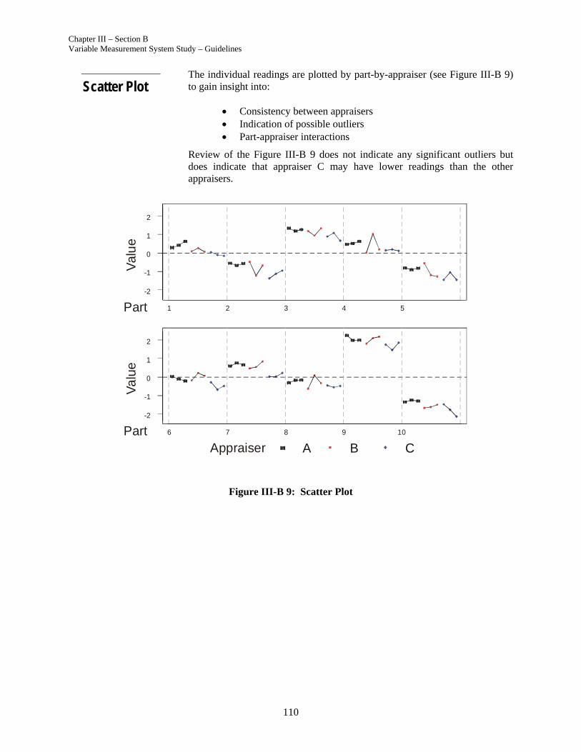
Chapter III – Section B Variable Measurement System Study – Guidelines
110
The individual readings are plotted by part-by-appraiser (see Figure III-B 9) to gain insight into:
Consistency between appraisers Indication of possible outliers Part-appraiser interactions
Review of the Figure III-B 9 does not indicate any significant outliers but does indicate that appraiser C may have lower readings than the other appraisers.
Figure III-B 9: Scatter Plot
Scatter Plot
-2
-1
0
1
2
1 2 3 4 5
-2
-1
0
1
2
6 7 8 9 10
Val
ue
Va
lue
A B C
Appraiser
Part
Part
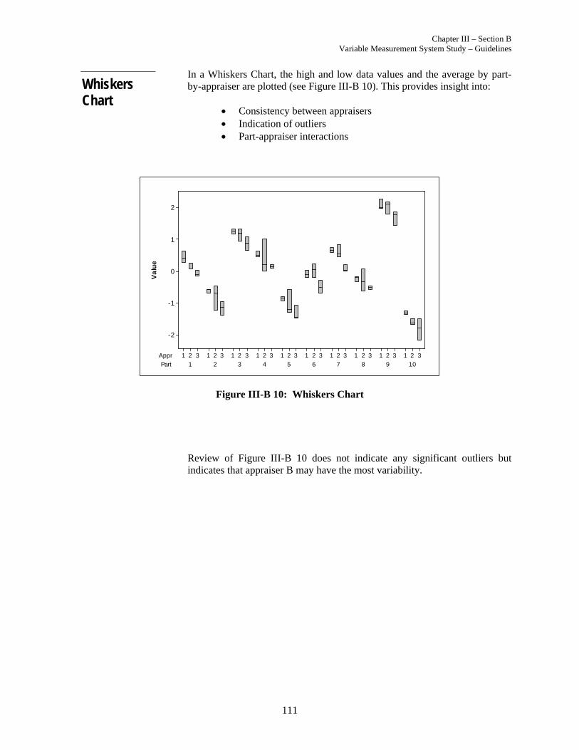
Chapter III – Section B Variable Measurement System Study – Guidelines
111
In a Whiskers Chart, the high and low data values and the average by part-by-appraiser are plotted (see Figure III-B 10). This provides insight into:
Consistency between appraisers Indication of outliers Part-appraiser interactions
PartAppr
10987654321321321321321321321321321321321
2
1
0
-1
-2
Val
ue
Figure III-B 10: Whiskers Chart
Review of Figure III-B 10 does not indicate any significant outliers but indicates that appraiser B may have the most variability.
Whiskers Chart
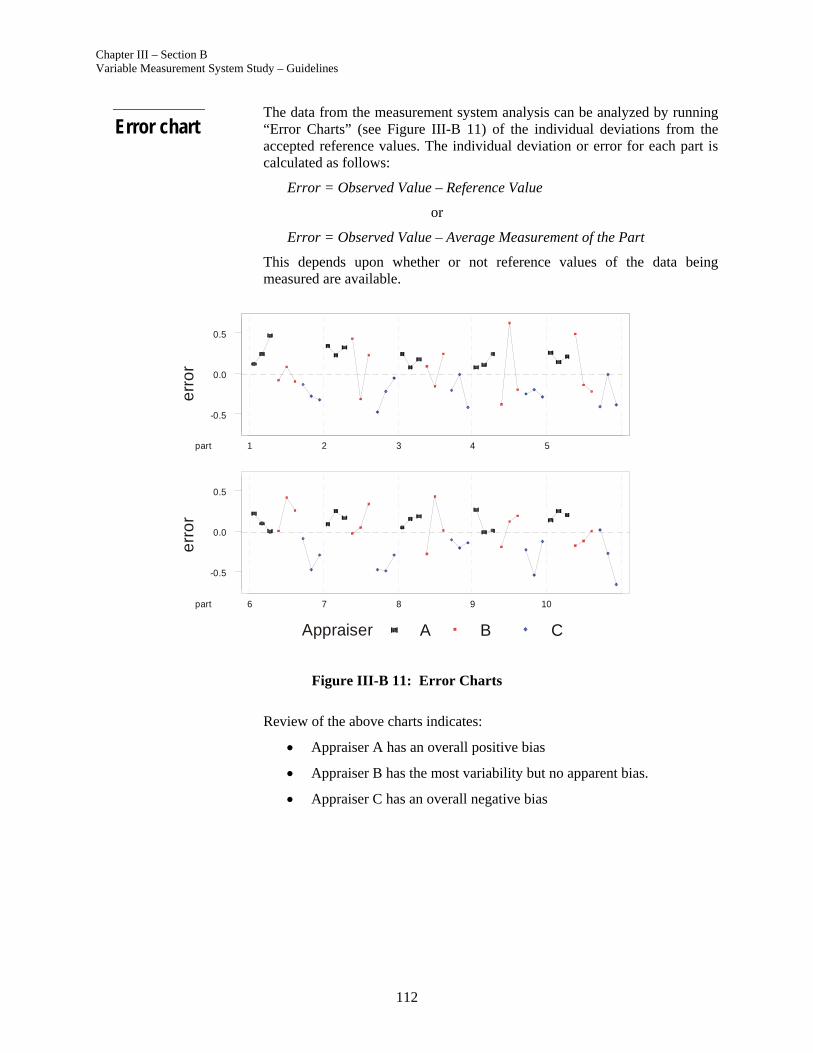
Chapter III – Section B Variable Measurement System Study – Guidelines
112
The data from the measurement system analysis can be analyzed by running “Error Charts” (see Figure III-B 11) of the individual deviations from the accepted reference values. The individual deviation or error for each part is calculated as follows:
Error = Observed Value – Reference Value
or
Error = Observed Value – Average Measurement of the Part
This depends upon whether or not reference values of the data being measured are available.
Figure III-B 11: Error Charts
Review of the above charts indicates:
Appraiser A has an overall positive bias
Appraiser B has the most variability but no apparent bias.
Appraiser C has an overall negative bias
Error chart
0.5
0.0
-0.5
543 2 1part
0.5
0.0
-0.5
1098 7 6part
A B C
Appraiser
err
or
err
or
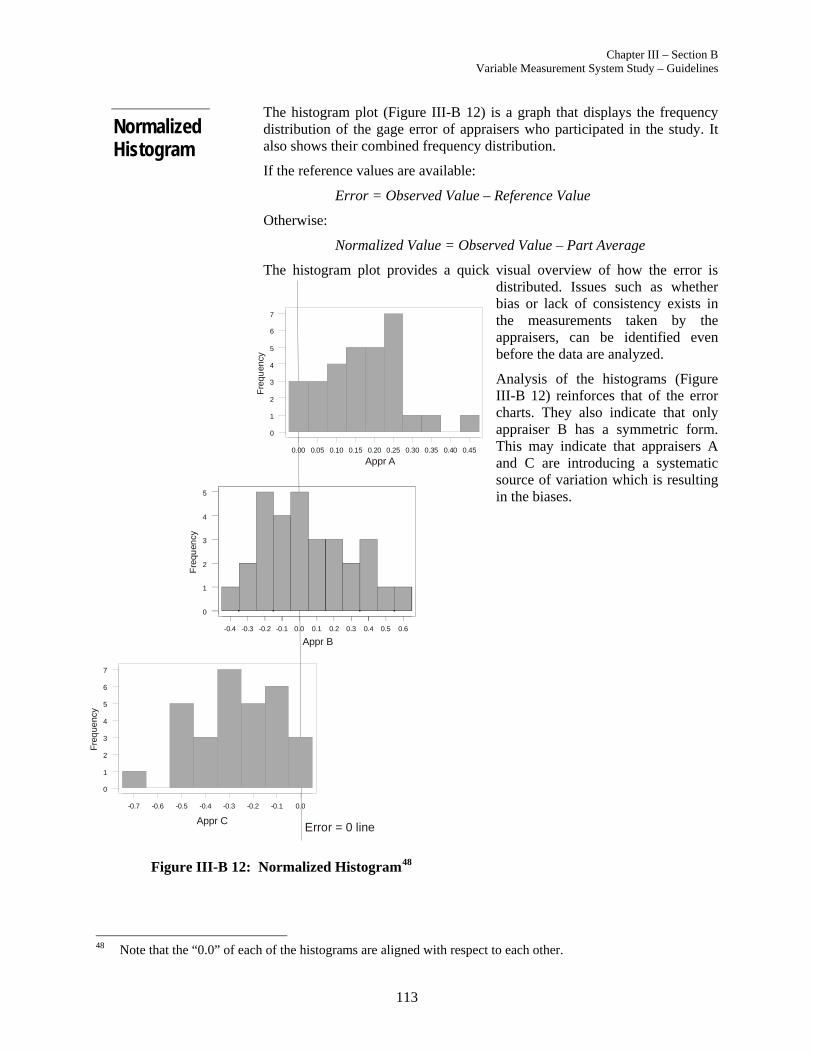
Chapter III – Section B Variable Measurement System Study – Guidelines
113
The histogram plot (Figure III-B 12) is a graph that displays the frequency distribution of the gage error of appraisers who participated in the study. It also shows their combined frequency distribution.
If the reference values are available:
Error = Observed Value – Reference Value
Otherwise:
Normalized Value = Observed Value – Part Average
The histogram plot provides a quick visual overview of how the error is distributed. Issues such as whether bias or lack of consistency exists in the measurements taken by the appraisers, can be identified even before the data are analyzed.
Analysis of the histograms (Figure III-B 12) reinforces that of the error charts. They also indicate that only appraiser B has a symmetric form. This may indicate that appraisers A and C are introducing a systematic source of variation which is resulting in the biases.
Figure III-B 12: Normalized Histogram P
48
48 Note that the “0.0” of each of the histograms are aligned with respect to each other.
Normalized Histogram
-0.7 -0.6 -0.5 -0.4 -0.3 -0.2 -0.1 0.0
0
1
2
3
4
5
6
7
Fre
que
ncy
-0.4 -0.3 -0.2 -0.1 0.0 0.1 0.2 0.3 0.4 0.5 0.6
0
1
2
3
4
5
Fre
quen
cy
0.00 0.05 0.10 0.15 0.20 0.25 0.30 0.35 0.40 0.45
0
1
2
3
4
5
6
7
Fre
quen
cy
Appr A
Appr B
Appr CError = 0 line
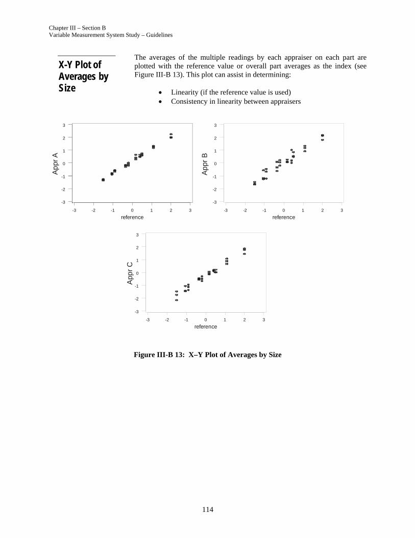
Chapter III – Section B Variable Measurement System Study – Guidelines
114
The averages of the multiple readings by each appraiser on each part are plotted with the reference value or overall part averages as the index (see Figure III-B 13). This plot can assist in determining:
Linearity (if the reference value is used) Consistency in linearity between appraisers
Figure III-B 13: X–Y Plot of Averages by Size
X-Y Plot of Averages by Size
3210-1-2-3
3
2
1
0
-1
-2
-3
reference
3210-1-2-3
3
2
1
0
-1
-2
-3
reference3210-1-2-3
3
2
1
0
-1
-2
-3
reference
Ap
pr A
Ap
pr B
App
r C
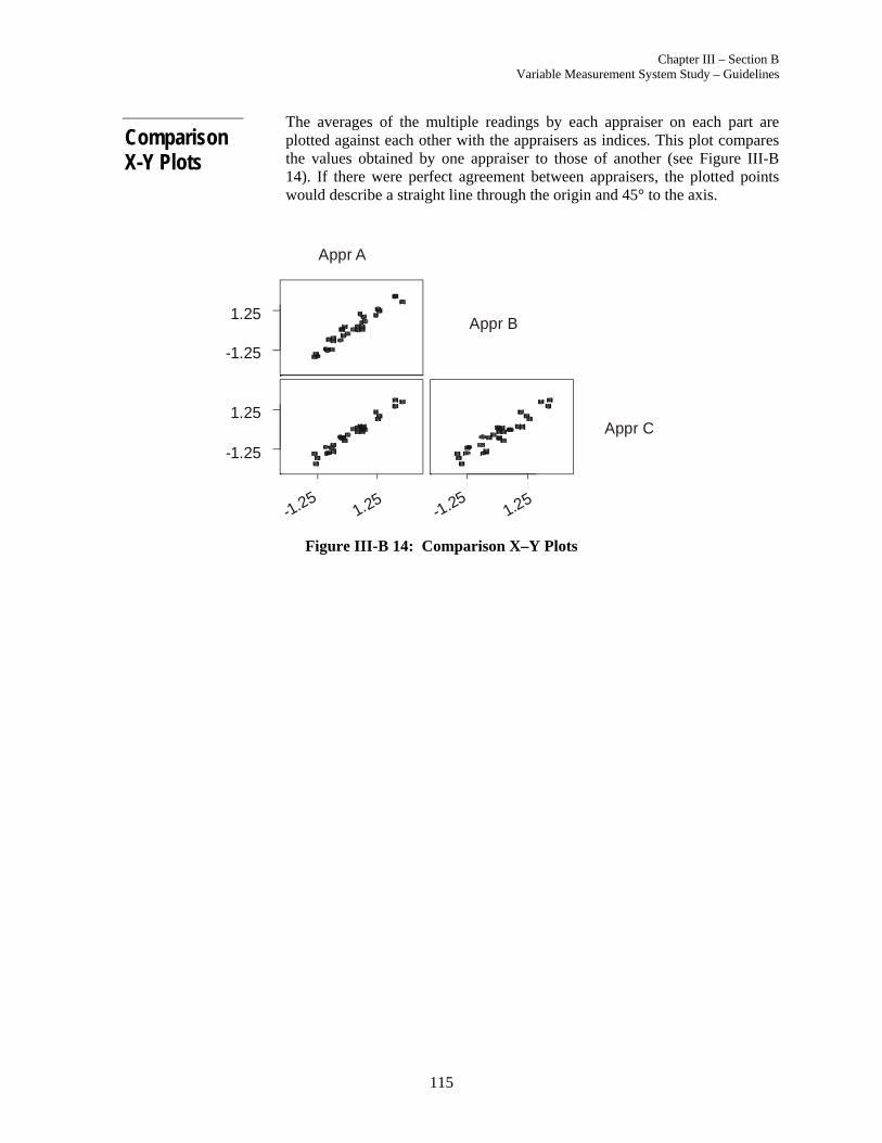
Chapter III – Section B Variable Measurement System Study – Guidelines
115
The averages of the multiple readings by each appraiser on each part are plotted against each other with the appraisers as indices. This plot compares the values obtained by one appraiser to those of another (see Figure III-B 14). If there were perfect agreement between appraisers, the plotted points would describe a straight line through the origin and 45° to the axis.
Figure III-B 14: Comparison X–Y Plots
Comparison X-Y Plots
1.25
-1.25
1.25-1.25
1.25
-1.25
1.25-1.25
Appr A
Appr B
Appr C

Chapter III – Section B Variable Measurement System Study – Guidelines
116
The Gage Repeatability and Reproducibility calculations are shown in Figures III-B 15 and III-B 16. Figure III-B 15 shows the data collection sheet on which all study results are recorded. Figure III-B 16 displays a report sheet on which all identifying information is to be recorded and all calculations made according to the prescribed formula.
Reproducible blank forms are available in the Sample Forms section. The procedure for doing the calculations after data have been collected is as follows:
(The following refers to Figure III-B 15) 1) Subtract the smallest reading from the largest reading in rows 1, 2
and 3; enter the result in row 5. Do the same for rows 6, 7, and 8; and 11, 12, and 13 and enter results in rows 10 and 15, respectively.
2) Entries in rows 5, 10 and 15 are ranges and therefore always positive values.
3) Total row 5 and divide the total by the number of parts sampled to
obtain the average range for the first appraisers trials aR . Do the
same for rows 10 and 15 to obtain bR and cR .
4) Transfer the averages of rows 5, 10, and 15 ( aR , bR , cR ) to row
17. Add them together and divide by the number of appraisers and
enter results R (average of all ranges).
5) Enter R (average value) in rows 19 and multiply by D4 P
49F to get
the upper control limit. Note: D4 is 3.27 if two trials are used. The value of the Upper Control Limit (UCLR ) of the individual ranges is entered in row 19. Note: The value of Lower Control Limit (LCLR) for less than seven trials is equal to zero.
6) Repeat any readings that produced a range greater than the calculated UCLR using the same appraiser and part as originally
used, or discard those values and re-average and recompute R and the limiting value UCLR based upon the revised sample size. Correct the special cause that produced the out-of-control condition. If the data were plotted and analyzed using a control chart as discussed previously, this condition would have already been corrected and would not occur here.
7) Sum the rows (rows 1, 2, 3, 6, 7, 8, 11, 12, and 13). Divide the sum in each row by the number of parts sampled and enter these values in the right-most column labeled “Average”.
49 See Statistical Process Control (SPC) Reference Manual, 2005, or other statistical reference source for a table
of factors.
Numerical Calculations
Chapter III – Section B Variable Measurement System Study – Guidelines
117
8) Add the averages in rows 1, 2 and 3 and divide the total by the
number of trials and enter the value in row 4 in the aX block.
Repeat this for rows 6, 7 and 8; and 11, 12 and 13, and enter the
results in the blocks for bX and cX in rows 9 and 14,
respectively.
9) Enter the maximum and minimum averages of rows 4, 9 and 14 in the appropriate space in row 18 and determine the differences.
Enter this difference in the space labeled DIFFX in row 18.
10) Sum the measurements for each trial, for each part, and divide the total by the number of measurements (number of trials times the number of appraisers). Enter the results in row 16 in the spaces provided for part average.
11) Subtract the smallest part average from the largest part average and enter the result in the space labeled pR in row 16. pR is the
range of part averages.
(The following refers to Figure III-B 16)
12) Transfer the calculated values of R , DIFFX and pR to the blanks
provided on the report side of the form.
13) Perform the calculations under the column entitled “Measurement Unit Analysis” on the left side of the form.
14) Perform the calculations under the column entitled “% Total Variation” on the right side of the form.
15) Check the results to make sure no errors have been made.
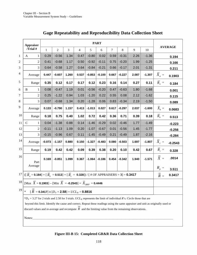
Chapter III – Section B Variable Measurement System Study – Guidelines
118
Figure III-B 15: Completed GR&R Data Collection Sheet
Gage Repeatability and Reproducibility Data Collection Sheet
PART
Appraiser /Trial # 1 2 3 4 5 6 7 8 9 10
AVERAGE
1 A 1 0.29 -0.56 1.34 0.47 -0.80 0.02 0.59 -0.31 2.26 -1.36 0.194
2 2 0.41 -0.68 1.17 0.50 -0.92 -0.11 0.75 -0.20 1.99 -1.25 0.166
3 3 0.64 -0.58 1.27 0.64 -0.84 -0.21 0.66 -0.17 2.01 -1.31 0.211
4 Average 0.447 -0.607 1.260 0.537 -0.853 -0.100 0.667 -0.227 2.087 -1.307 aX = 0.1903
5 Range 0.35 0.12 0.17 0.17 0.12 0.23 0.16 0.14 0.27 0.11 aR = 0.184
6 B 1 0.08 -0.47 1.19 0.01 -0.56 -0.20 0.47 -0.63 1.80 -1.68 0.001
7 2 0.25 -1.22 0.94 1.03 -1.20 0.22 0.55 0.08 2.12 -1.62 0.115
8 3 0.07 -0.68 1.34 0.20 -1.28 0.06 0.83 -0.34 2.19 -1.50 0.089
9 Average 0.133 -0.790 1.157 0.413 -1.013 0.027 0.617 -0.297 2.037 -1.600 bX = 0.0683
10 Range 0.18 0.75 0.40 1.02 0.72 0.42 0.36 0.71 0.39 0.18 bR = 0.513
11 C 1 0.04 -1.38 0.88 0.14 -1.46 -0.29 0.02 -0.46 1.77 -1.49 -0.223
12 2 -0.11 -1.13 1.09 0.20 -1.07 -0.67 0.01 -0.56 1.45 -1.77 -0.256
13 3 -0.15 -0.96 0.67 0.11 -1.45 -0.49 0.21 -0.49 1.87 -2.16 -0.284
14 Average -0.073 -1.157 0.880 0.150 -1.327 -0.483 0.080 -0.503 1.697 -1.807 cX = -0.2543
15 Range 0.19 0.42 0.42 0.09 0.39 0.38 0.20 0.10 0.42 0.67 cR = 0.328
16 Part
Average
0.169
-0.851
1.099
0.367 -1.064 -0.186 0.454 -0.342 1.940
-1.571
X =
pR =
.0014
3.511
17 ([aR = 0.184] + [
bR = 0.513] + [cR = 0.328]) / [ # OF APPRAISERS = 3] = 0.3417 R = 0.3417
18 [Max X = 0.1903] – [Min X = -0.2543] = DIFFX = 0.4446
19 * [ R = 0.3417] x [D4 = 2.58] = UCLR = 0.8816
*D4 = 3.27 for 2 trials and 2.58 for 3 trials. UCLR represents the limit of individual R’s. Circle those that are
beyond this limit. Identify the cause and correct. Repeat these readings using the same appraiser and unit as originally used or
discard values and re-average and recompute R and the limiting value from the remaining observations.
Notes:_____________________________________________________________________________________________________________
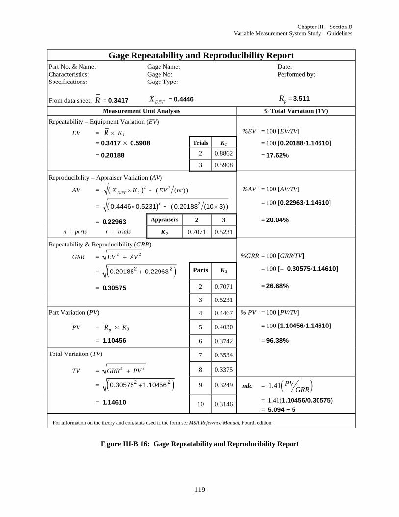
Chapter III – Section B Variable Measurement System Study – Guidelines
119
Figure III-B 16: Gage Repeatability and Reproducibility Report
Gage Repeatability and Reproducibility Report Part No. & Name: Characteristics: Specifications:
From data sheet: R = 0.3417
Gage Name: Gage No: Gage Type:
DIFFX = 0.4446
Date: Performed by:
pR = 3.511
Measurement Unit Analysis % Total Variation (TV)
Repeatability – Equipment Variation (EV)
EV = R K1 %EV = 100 [EV/TV]
= 0.3417 0.5908 Trials K1 = 100 [0.20188/1.14610]
= 0.20188 2 0.8862 = 17.62% 3 0.5908
Reproducibility – Appraiser Variation (AV)
AV = 2 2
2 ( ( ) )-DIFFX K EV nr %AV = 100 [AV/TV]
= 2 20.4446 0.5231 ( 0.20188 (10 3) )-
= 100 [0.22963/1.14610]
= 0.22963 Appraisers 2 3 = 20.04%
n = parts r = trials K2 0.7071 0.5231
Repeatability & Reproducibility (GRR)
GRR = 2 2 EV AV
%GRR = 100 [GRR/TV]
= 2 20.20188 0.22963 Parts K3 = 100 [= 0.30575/1.14610]
= 0.30575 2 0.7071 = 26.68%
3 0.5231
Part Variation (PV) 4 0.4467 % PV = 100 [PV/TV]
PV = pR K3 5 0.4030 = 100 [1.10456/1.14610]
= 1.10456 6 0.3742 = 96.38%
Total Variation (TV) 7 0.3534
TV = 2 2 GRR PV 8 0.3375
= 2 20.30575 1.10456 9 0.3249 ndc = 1.41 PVGRR
= 1.14610 10 0.3146 = 1.41(1.10456/0.30575)
= 5.094 ~ 5
For information on the theory and constants used in the form see MSA Reference Manual, Fourth edition.
Chapter III – Section B Variable Measurement System Study – Guidelines
120
The Gage Repeatability and Reproducibility Data Collection Sheet and Report forms, Figures III-B 15 and III-B 16, will provide a method for the numerical analysis of the study data P
50F. The analysis will estimate the
variation and percent of process variation for the total measurement system and its components repeatability, reproducibility, and part variation. This information needs to be compared to and complement the results of the graphical analysis.
On the left side of the form (Figure III-B 16) under Measurement Unit Analysis, the standard deviation is calculated for each component of variation.
The repeatability or equipment variation (EV or E ) is determined by
multiplying the average range ( R ) by a constant (K1). K1 depends upon the
number of trials used in the gage study and is equal to the inverse of *2d
which is obtained from Appendix C. *2d is dependent on the number of trials
(m) and the number of parts times the number of appraisers (g) (assumed to be greater than 15 for calculating the value of K1)
The reproducibility or appraiser variation (AV or A ) is determined by
multiplying the maximum average appraiser difference ( X DIFF ) by a constant (K2 ). K2 depends upon the number of appraisers used in the gage
study and is the inverse of *2d which is obtained from Appendix C. *
2d is dependent on the number of appraisers (m) and g = 1, since there is only one range calculation. Since the appraiser variation is contaminated by the equipment variation, it must be adjusted by subtracting a fraction of the equipment variation. Therefore, the appraiser variation (AV) is calculated by
22
2 DIFF
EVAV X K
nr
where n = number of parts and r = number of trials.
If a negative value is calculated under the square root sign, the appraiser variation (AV) defaults to zero.
The measurement system variation for repeatability and reproducibility (GRR or M ) is calculated by adding the square of the equipment variation and the square of the appraiser variation, and taking the square root as follows:
2 2 ( ) ( )GRR EV AV
There are generally four different approaches to determine the process variation which is used to analyze the acceptability of the measurement variation:
50 The numerical results in the example were developed as if they were computed manually; i.e., the results were
carried and rounded to one additional decimal digit. Analysis by computer programs should maintain the intermediate values to the maximum precision of the computer/programming language. The results from a valid computer program may differ from the example results in the second or greater decimal place but the final analysis will remain the same.
Analysis of Results — Numerical
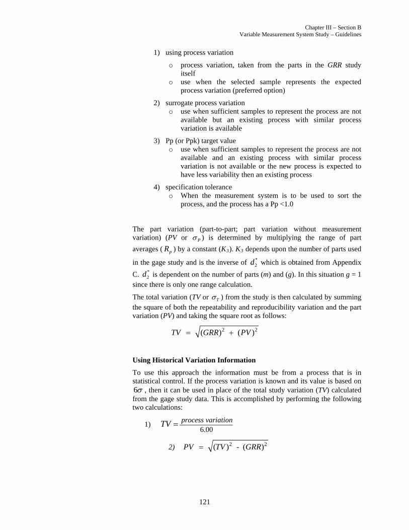
Chapter III – Section B Variable Measurement System Study – Guidelines
121
1) using process variation
o process variation, taken from the parts in the GRR study itself
o use when the selected sample represents the expected process variation (preferred option)
2) surrogate process variation o use when sufficient samples to represent the process are not
available but an existing process with similar process variation is available
3) Pp (or Ppk) target value o use when sufficient samples to represent the process are not
available and an existing process with similar process variation is not available or the new process is expected to have less variability then an existing process
4) specification tolerance o When the measurement system is to be used to sort the
process, and the process has a Pp <1.0
The part variation (part-to-part; part variation without measurement variation) (PV or P ) is determined by multiplying the range of part
averages ( pR ) by a constant (K3). K3 depends upon the number of parts used
in the gage study and is the inverse of *2d which is obtained from Appendix
C. *2d is dependent on the number of parts (m) and (g). In this situation g = 1
since there is only one range calculation.
The total variation (TV or T ) from the study is then calculated by summing the square of both the repeatability and reproducibility variation and the part variation (PV) and taking the square root as follows:
2 2 ( ) ( )TV GRR PV
Using Historical Variation Information
To use this approach the information must be from a process that is in statistical control. If the process variation is known and its value is based on 6 , then it can be used in place of the total study variation (TV) calculated from the gage study data. This is accomplished by performing the following two calculations:
1) 6.00
process variationTV
2) 2 2 ( ) - ( )PV TV GRR

Chapter III – Section B Variable Measurement System Study – Guidelines
122
Using a Pp (or Ppk) target value
To use the Pp option, use the following TV in the GRR analysis:
6 6 6
6
pP
USL LSL USL LSL USL LSLsince P
s TV
USL LSLthen TV
Pp
and 2 2 ( ) - ( )PV TV GRR
Using the Tolerance (Specification Range).
When comparing measurement error from a GRR study to a tolerance, this is the same as comparing it to a production process with a Pp of 1.00. OEM customers rarely expect process variation to have as low a Pp(k) as 1.00, nor do they accept a process at that low of a performance level. It may make more sense to compare the measurement variation to a target production process performance level which meets the customer requirement. P
51
To use this option, use the following TV in the GRR analysis:
6
USL LSLTV
and 2 2 ( ) - ( )PV TV GRR
Indices
Once the variability for each factor in the gage study is determined, it can be compared to the total variation (TV). This is accomplished by performing the calculations on the right side of the gage report form (Figure III-B 16) under “% Total Variation.”
The percent the equipment variation (%EV) consumes of the total variation (TV) is calculated by 100[EV/TV]. The percent that the other factors consume of the total variation can be similarly calculated as follows:
%AV = 100 [AV/TV]
%GRR = 100 [GRR/TV]
%PV = 100 [PV/TV]
THE SUM OF THE PERCENT CONSUMED BY EACH FACTOR WILL NOT EQUAL 100%.
The results of this percent total variation need to be evaluated to determine if the measurement system is acceptable for its intended application.
51 for example, see Chrysler, Ford, and GM, PPAP Manual.

Chapter III – Section B Variable Measurement System Study – Guidelines
123
If the analysis is based on the tolerance instead of the process variation, then the Gage Repeatability and Reproducibility Report form (Figure III-B 16) can be modified so that the right-hand side of the form represents the percent of tolerance instead of percent of total variation. In that case, %EV, %AV, %GRR and %PV are calculated by substituting the value of tolerance divided by six in the denominator of the calculations in place of the total variation (TV). Either or both approaches can be taken depending on the intended use of the measurement system and the desires of the customer.
The final step in the numerical analysis is to determine the number of distinct categories that can be reliably distinguished by the measurement system. This is the number of non-overlapping 97% confidence intervals that will span the expected product variation. P
52F
1.41 PVndc GRR
Given that the graphical analysis has not indicated any special cause variation, the rule of thumb for gage repeatability and reproducibility (%GRR) may be found in Chapter II, Section D.
For analysis, the ndc is the maximum of one or the calculated value truncated to the integer. This result should be greater than or equal to 5.
To avoid a ndc = 0, which is possible with truncation alone, some computer programs will round up the calculated result. This can result in differences in final reports when the same data is evaluated by different programs
When using the Pp approach to TV, the calculation for ndc is:
. .
TV PV GRR
or PV TV GRR
then
TV GRRPVndc
GRR GRR
2 2 2
2 2 2
2 2
1 41 1 41
Analysis of Variance (ANOVA) Method
Analysis of variance (ANOVA) is a standard statistical technique and can be used to analyze the measurement error and other sources of variability of data in a measurement systems study. In the analysis of variance, the variance can be decomposed into four categories: parts, appraisers, interaction between parts and appraisers, and replication error due to the gage.
52 The importance of the number of distinct categories (ndc) in control and analysis activities is discussed in
Chapter I, Section E, "Measurement Issues" (especially Figure I-E 3). Calculation of ndc is reviewed in Chapter II, Section B, "Analysis of Results - Numerical".
Chapter III – Section B Variable Measurement System Study – Guidelines
124
The advantages of ANOVA techniques as compared with Average and Range methods are:
They are capable of handling any experimental set-up
Can estimate the variances more accurately
Extract more information (such as interaction between parts and appraisers effect) from the experimental data.
The disadvantages are that the numerical computations are more complex and users require a certain degree of statistical knowledge to interpret the results. The ANOVA method as described in the following sections is advised, especially if a computer is available.
The method of collecting the data is important in an ANOVA method. If the data are not collected in a random manner, this can lead to a source of bias values. A simple way to assure a balanced design for (n) parts, (k) appraisers, and (r) trials is through randomization. One common approach to randomization is to write A1 on a slip of paper to denote the measurement for the first appraiser on the first part. Do this up to A(n) for the measurement by the first appraiser on the nth part. Follow the same procedure for the next appraiser up to and including the kth appraiser. The similar notation will be used where B1, C1 denotes the measurement for second and third appraiser on the first part. Once all nk combinations are written, then the slips of paper can be put in a hat or bowl. One at a time, a slip of paper is selected. These combinations (A1, B2, ...) are the measuring order in which the gage study will be performed. Once all nk combinations are selected, they are put back into the hat and the procedure is followed again. This is done for a total of r times to determine the order of experiments for each repeat.
There are alternate approaches to generate a random sample. Care should be exercised to differentiate among random, haphazard and convenience sampling. P
53F P
54
In general, all efforts need to be taken to assure statistical independence within the study.
Conducting the Study
The data can be collected in a random manner using a form similar to Table III-B 6a. For our example, there are ten parts and three appraisers, and the experiment has been performed in random order three times for each part and appraiser combination.
53 See Wheeler and Lyday, Evaluating the Measurement Process, Second Edition, 1989, p. 27. 54 Robert R. Coveyou (1915 - 20 Feb 1996) was an American mathematician who was a health physicist with the
Manhattan Project from 1943 during WW II. He became a recognized expert in pseudo-random number generators.
Randomization and Statistical Independence
“The generation of random numbers is too important to be left to chance.”
Robert R. Coveyou56
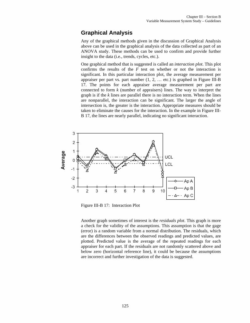
Chapter III – Section B Variable Measurement System Study – Guidelines
125
Graphical Analysis Any of the graphical methods given in the discussion of Graphical Analysis above can be used in the graphical analysis of the data collected as part of an ANOVA study. These methods can be used to confirm and provide further insight to the data (i.e., trends, cycles, etc.).
One graphical method that is suggested is called an interaction plot. This plot confirms the results of the F test on whether or not the interaction is significant. In this particular interaction plot, the average measurement per appraiser per part vs. part number (1, 2, … etc.) is graphed in Figure III-B 17. The points for each appraiser average measurement per part are connected to form k (number of appraisers) lines. The way to interpret the graph is if the k lines are parallel there is no interaction term. When the lines are nonparallel, the interaction can be significant. The larger the angle of intersection is, the greater is the interaction. Appropriate measures should be taken to eliminate the causes for the interaction. In the example in Figure III-B 17, the lines are nearly parallel, indicating no significant interaction.
Figure III-B 17: Interaction Plot
Another graph sometimes of interest is the residuals plot. This graph is more a check for the validity of the assumptions. This assumption is that the gage (error) is a random variable from a normal distribution. The residuals, which are the differences between the observed readings and predicted values, are plotted. Predicted value is the average of the repeated readings for each appraiser for each part. If the residuals are not randomly scattered above and below zero (horizontal reference line), it could be because the assumptions are incorrect and further investigation of the data is suggested.
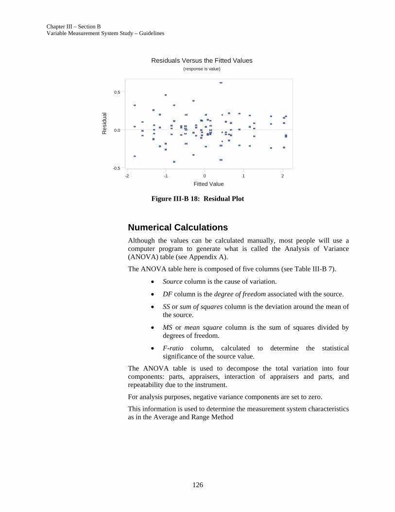
Chapter III – Section B Variable Measurement System Study – Guidelines
126
Figure III-B 18: Residual Plot
Numerical Calculations Although the values can be calculated manually, most people will use a computer program to generate what is called the Analysis of Variance (ANOVA) table (see Appendix A).
The ANOVA table here is composed of five columns (see Table III-B 7).
Source column is the cause of variation.
DF column is the degree of freedom associated with the source.
SS or sum of squares column is the deviation around the mean of the source.
MS or mean square column is the sum of squares divided by degrees of freedom.
F-ratio column, calculated to determine the statistical significance of the source value.
The ANOVA table is used to decompose the total variation into four components: parts, appraisers, interaction of appraisers and parts, and repeatability due to the instrument.
For analysis purposes, negative variance components are set to zero.
This information is used to determine the measurement system characteristics as in the Average and Range Method
210-1-2
0.5
0.0
-0.5
Fitted Value
Re
sidu
al
Residuals Versus the Fitted Values(response is value)
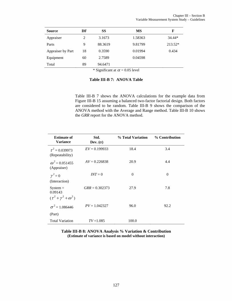
Chapter III – Section B Variable Measurement System Study – Guidelines
127
Source DF SS MS F
Appraiser 2 3.1673 1.58363 34.44*
Parts 9 88.3619 9.81799 213.52*
Appraiser by Part 18 0.3590 0.01994 0.434
Equipment 60 2.7589 0.04598
Total 89 94.6471
* Significant at = 0.05 level
Table III-B 7: ANOVA Table
Table III-B 7 shows the ANOVA calculations for the example data from Figure III-B 15 assuming a balanced two-factor factorial design. Both factors are considered to be random. Table III-B 9 shows the comparison of the ANOVA method with the Average and Range method. Table III-B 10 shows the GRR report for the ANOVA method.
Estimate of Variance
Std. Dev. ()
% Total Variation % Contribution
2 = 0.039973 (Repeatability)
EV = 0.199933 18.4 3.4
2 = 0.051455 (Appraiser)
AV = 0.226838 20.9 4.4
2 = 0
(Interaction)
INT = 0 0 0
System = 0.09143
( 2 2 2 )
GRR = 0.302373 27.9 7.8
2 = 1.086446
(Part)
PV = 1.042327 96.0 92.2
Total Variation TV =1.085 100.0
Table III-B 8: ANOVA Analysis % Variation & Contribution (Estimate of variance is based on model without interaction)

Chapter III – Section B Variable Measurement System Study – Guidelines
128
1.04233 1.41 4.861 5.30237 ndc
2 2 ( ) Total Variation TV GRR PV
( )
( )
% 100 components
total
of TotalVariation
2( )
2( )
% ( ) 100components
totalContribution to Total Variance
Analysis of GRR Studies Both the Average and Range method and ANOVA method will provide information concerning the causes of measurement system or gage variation.
For example, if repeatability is large compared to reproducibility, the reasons may be:
The instrument needs maintenance.
The gage may need to be redesigned to be more rigid.
The clamping or location for gaging needs to be improved.
There is excessive within-part variation.
If reproducibility is large compared to repeatability, then possible causes could be:
The appraiser needs to be better trained in how to use and read the gage instrument.
Calibrations on the gage dial are not clear.
A fixture of some sort may be needed to help the appraiser use the gage more consistently.

Chapter III – Section B Variable Measurement System Study – Guidelines
129
Method Lower
90% CL P
55 Std. Dev. Upper
90% CL % of Total Variation
GRR* EV 0.175 .202 0.240 17.6 AV 0.133 .230 1.016 20.1 INTERACTION -- na -- na GRR 0.266 .306 0.363 26.7 PV 1.104 96.4
UANOVA
EV 0.177 0.200 0.231 18.4 AV 0.129 0.227 1.001 20.9 INTERACTION -- 0 -- 0 GRR 0.237 0.302 1.033 27.9 PV 1.042 96.0
* In the average and range method, the interaction component cannot be estimated.
Table III-B 9: Comparison of ANOVA and Average and Range Methods
Part No. & Name: Characteristics: Specifications:
Gage Name: Gage No: Gage Type:
Date: Performed by:
STD. DEV. % TOTAL
VARIATION PERCENT
CONTRIBUTION Repeatability (EV) 0.200 18.4 3.4 Reproducibility (AV) 0.227 20.9 4.4 Appraiser by Part (INT) 0 0 0 GRR 0.302 27.9 7.9 Part (PV) 1.042 96.0 92.2
Measurement System is acceptable for Process Control and Analysis. Note: Tolerance = N.A. Number of distinct data categories (ndc) = 4
Total variation (TV) = 1.085
Table III-B 10: GRR ANOVA Method Report
55 CL = Confidence Limit

Chapter III – Section B Variable Measurement System Study – Guidelines
130
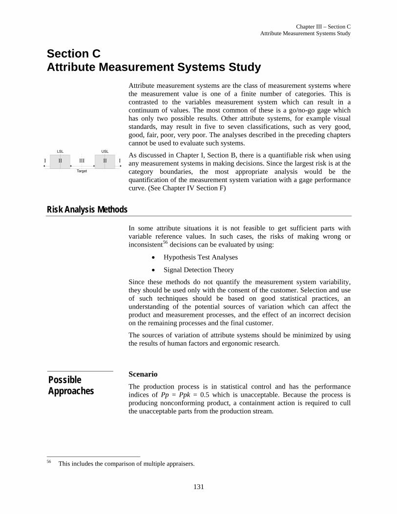
Chapter III – Section C Attribute Measurement Systems Study
131
Section C Attribute Measurement Systems Study
Attribute measurement systems are the class of measurement systems where the measurement value is one of a finite number of categories. This is contrasted to the variables measurement system which can result in a continuum of values. The most common of these is a go/no-go gage which has only two possible results. Other attribute systems, for example visual standards, may result in five to seven classifications, such as very good, good, fair, poor, very poor. The analyses described in the preceding chapters cannot be used to evaluate such systems.
As discussed in Chapter I, Section B, there is a quantifiable risk when using any measurement systems in making decisions. Since the largest risk is at the category boundaries, the most appropriate analysis would be the quantification of the measurement system variation with a gage performance curve. (See Chapter IV Section F)
Risk Analysis Methods
In some attribute situations it is not feasible to get sufficient parts with variable reference values. In such cases, the risks of making wrong or inconsistent P
56F decisions can be evaluated by using:
Hypothesis Test Analyses
Signal Detection Theory
Since these methods do not quantify the measurement system variability, they should be used only with the consent of the customer. Selection and use of such techniques should be based on good statistical practices, an understanding of the potential sources of variation which can affect the product and measurement processes, and the effect of an incorrect decision on the remaining processes and the final customer.
The sources of variation of attribute systems should be minimized by using the results of human factors and ergonomic research.
Scenario
The production process is in statistical control and has the performance indices of Pp = Ppk = 0.5 which is unacceptable. Because the process is producing nonconforming product, a containment action is required to cull the unacceptable parts from the production stream.
56 This includes the comparison of multiple appraisers.
Possible Approaches
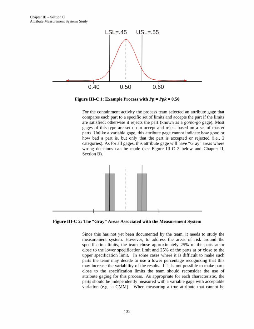
Chapter III – Section C Attribute Measurement Systems Study
132
Figure III-C 1: Example Process with Pp = Ppk = 0.50
For the containment activity the process team selected an attribute gage that compares each part to a specific set of limits and accepts the part if the limits are satisfied; otherwise it rejects the part (known as a go/no-go gage). Most gages of this type are set up to accept and reject based on a set of master parts. Unlike a variable gage, this attribute gage cannot indicate how good or how bad a part is, but only that the part is accepted or rejected (i.e., 2 categories). As for all gages, this attribute gage will have “Gray” areas where wrong decisions can be made (see Figure III-C 2 below and Chapter II, Section B).
Figure III-C 2: The “Gray” Areas Associated with the Measurement System
Since this has not yet been documented by the team, it needs to study the measurement system. However, to address the areas of risk around the specification limits, the team chose approximately 25% of the parts at or close to the lower specification limit and 25% of the parts at or close to the upper specification limit. In some cases where it is difficult to make such parts the team may decide to use a lower percentage recognizing that this may increase the variability of the results. If it is not possible to make parts close to the specification limits the team should reconsider the use of attribute gaging for this process. As appropriate for each characteristic, the parts should be independently measured with a variable gage with acceptable variation (e.g., a CMM). When measuring a true attribute that cannot be
LSL=.45 USL=.55
0.50 0.60 0.40

Chapter III – Section C Attribute Measurement Systems Study
133
measured with a variable gauge use other means such as experts to pre-determine which samples are good or defective.
Three appraisers are used, with each appraiser making three decisions on the each part.
An acceptable decision was designated with a one (1) and an unacceptable decision with zero (0). The reference decision and variable reference values shown in Table III-C 1 were not initially determined. The table also indicates in the “Coded” column whether the part is area I, area II, or area III part indicated by “– ”, “x”, and “+” respectively.
Hypothesis Test Analyses – Cross-Tab Method Since the team did not know the reference decisions for the parts, they developed cross-tabulations comparing each of the appraisers to the other.
The cross-tabulation process analyzes distribution data for two or more categorical variables. The results – presented in a matrix format – form a contingency table that illustrates the interdependency between variables. P
57F
57 Cross-tabulation is available in many statistical analysis software packages and is used in spreadsheet pivot
table functions.
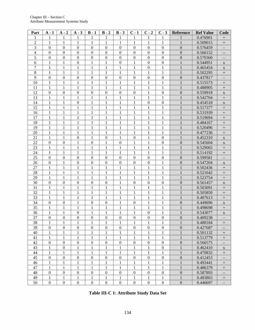
Chapter III – Section C Attribute Measurement Systems Study
134
Part A - 1 A - 2 A - 3 B - 1 B - 2 B - 3 C - 1 C - 2 C - 3 Reference Ref Value Code 1 1 1 1 1 1 1 1 1 1 1 0.476901 + 2 1 1 1 1 1 1 1 1 1 1 0.509015 + 3 0 0 0 0 0 0 0 0 0 0 0.576459 – 4 0 0 0 0 0 0 0 0 0 0 0.566152 – 5 0 0 0 0 0 0 0 0 0 0 0.570360 – 6 1 1 0 1 1 0 1 0 0 1 0.544951 x 7 1 1 1 1 1 1 1 0 1 1 0.465454 x 8 1 1 1 1 1 1 1 1 1 1 0.502295 + 9 0 0 0 0 0 0 0 0 0 0 0.437817 –
10 1 1 1 1 1 1 1 1 1 1 0.515573 + 11 1 1 1 1 1 1 1 1 1 1 0.488905 + 12 0 0 0 0 0 0 0 1 0 0 0.559918 x 13 1 1 1 1 1 1 1 1 1 1 0.542704 + 14 1 1 0 1 1 1 1 0 0 1 0.454518 x 15 1 1 1 1 1 1 1 1 1 1 0.517377 + 16 1 1 1 1 1 1 1 1 1 1 0.531939 + 17 1 1 1 1 1 1 1 1 1 1 0.519694 + 18 1 1 1 1 1 1 1 1 1 1 0.484167 + 19 1 1 1 1 1 1 1 1 1 1 0.520496 + 20 1 1 1 1 1 1 1 1 1 1 0.477236 + 21 1 1 0 1 0 1 0 1 0 1 0.452310 x 22 0 0 1 0 1 0 1 1 0 0 0.545604 x 23 1 1 1 1 1 1 1 1 1 1 0.529065 + 24 1 1 1 1 1 1 1 1 1 1 0.514192 + 25 0 0 0 0 0 0 0 0 0 0 0.599581 – 26 0 1 0 0 0 0 0 0 1 0 0.547204 x 27 1 1 1 1 1 1 1 1 1 1 0.502436 + 28 1 1 1 1 1 1 1 1 1 1 0.521642 + 29 1 1 1 1 1 1 1 1 1 1 0.523754 + 30 0 0 0 0 0 1 0 0 0 0 0.561457 x 31 1 1 1 1 1 1 1 1 1 1 0.503091 + 32 1 1 1 1 1 1 1 1 1 1 0.505850 + 33 1 1 1 1 1 1 1 1 1 1 0.487613 + 34 0 0 1 0 0 1 0 1 1 0 0.449696 x 35 1 1 1 1 1 1 1 1 1 1 0.498698 + 36 1 1 0 1 1 1 1 0 1 1 0.543077 x 37 0 0 0 0 0 0 0 0 0 0 0.409238 – 38 1 1 1 1 1 1 1 1 1 1 0.488184 + 39 0 0 0 0 0 0 0 0 0 0 0.427687 – 40 1 1 1 1 1 1 1 1 1 1 0.501132 + 41 1 1 1 1 1 1 1 1 1 1 0.513779 + 42 0 0 0 0 0 0 0 0 0 0 0.566575 – 43 1 0 1 1 1 1 1 1 0 1 0.462410 x 44 1 1 1 1 1 1 1 1 1 1 0.470832 + 45 0 0 0 0 0 0 0 0 0 0 0.412453 – 46 1 1 1 1 1 1 1 1 1 1 0.493441 + 47 1 1 1 1 1 1 1 1 1 1 0.486379 + 48 0 0 0 0 0 0 0 0 0 0 0.587893 – 49 1 1 1 1 1 1 1 1 1 1 0.483803 + 50 0 0 0 0 0 0 0 0 0 0 0.446697 –
Table III-C 1: Attribute Study Data Set
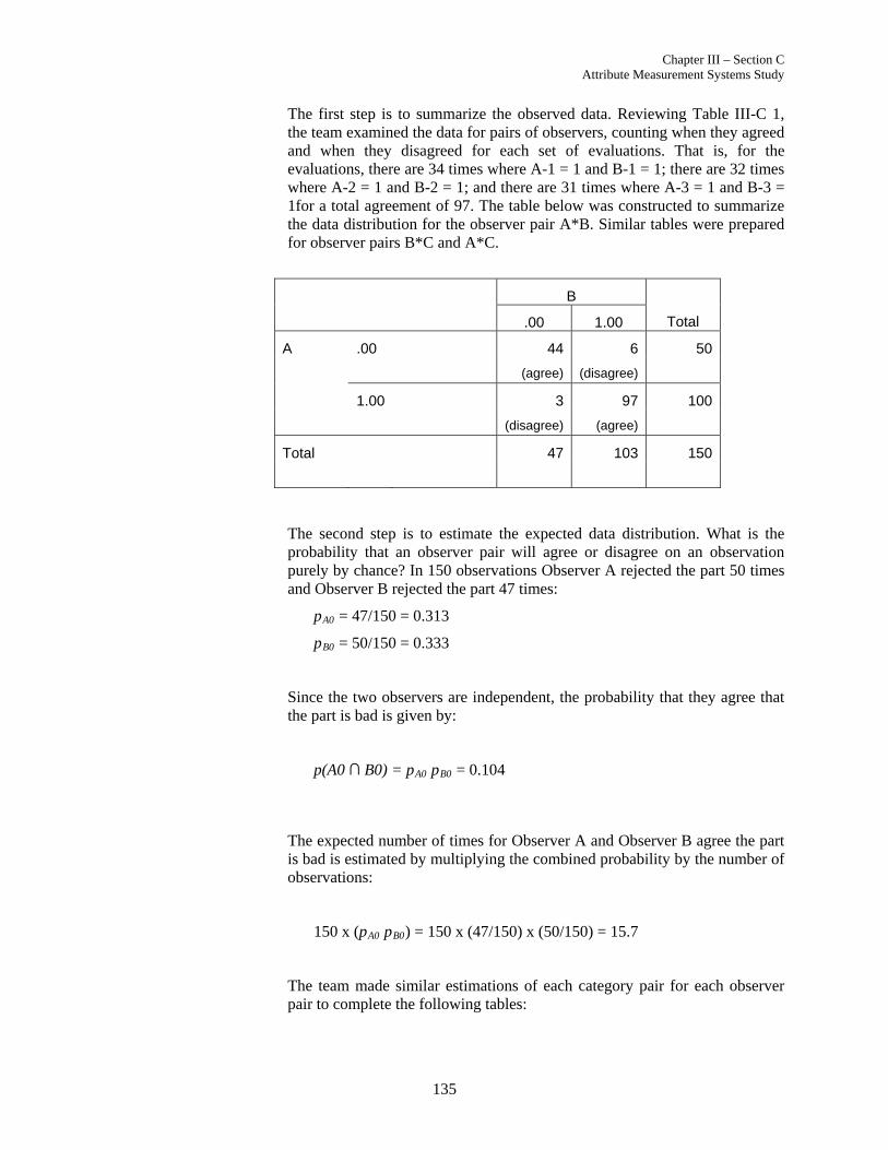
Chapter III – Section C Attribute Measurement Systems Study
135
The first step is to summarize the observed data. Reviewing Table III-C 1, the team examined the data for pairs of observers, counting when they agreed and when they disagreed for each set of evaluations. That is, for the evaluations, there are 34 times where A-1 = 1 and B-1 = 1; there are 32 times where A-2 = 1 and B-2 = 1; and there are 31 times where A-3 = 1 and B-3 = 1for a total agreement of 97. The table below was constructed to summarize the data distribution for the observer pair A*B. Similar tables were prepared for observer pairs B*C and A*C.
B
.00 1.00
Total
A .00 44 6 50
(agree) (disagree)
1.00 3 97 100
(disagree) (agree)
Total 47 103 150
The second step is to estimate the expected data distribution. What is the probability that an observer pair will agree or disagree on an observation purely by chance? In 150 observations Observer A rejected the part 50 times and Observer B rejected the part 47 times:
pA0 = 47/150 = 0.313
pB0 = 50/150 = 0.333
Since the two observers are independent, the probability that they agree that the part is bad is given by:
p(A0 ∩ B0) = pA0 pB0 = 0.104
The expected number of times for Observer A and Observer B agree the part is bad is estimated by multiplying the combined probability by the number of observations:
150 x (pA0 pB0) = 150 x (47/150) x (50/150) = 15.7
The team made similar estimations of each category pair for each observer pair to complete the following tables:

Chapter III – Section C Attribute Measurement Systems Study
136
Table III-C 2: Cross tabulation Study Results
To determine the level of this agreement the team uses the (Cohen's) kappa which measures the agreement between the evaluations of two raters when both are rating the same object. A value of 1 indicates perfect agreement. A value of 0 indicates that agreement is no better than chance. Kappa is only available for tables in which both variables use the same category values and both variables have the same number of categories. P
58
58 There are a number of statistics which can be used to determine inter-rater agreement. Different statistics are
appropriate for different types of measurement. See Reference List including: Bland, J. M., and Altman, D. G. (1986); Cohen, J. (1960); Everitt, B. (1996); Fleiss, J. L. (1971); Krippendorff, K. (2004); Saal, F.E., Downey, R.G. and Lahey, M.A. (1980); Shrout, P. and Fleiss, J. L. (1979); and Uebersax, John S. (1987)
A * B Crosstabulation
44 6 50
15.7 34.3 50.0
3 97 100
31.3 68.7 100.0
47 103 150
47.0 103.0 150.0
Count
Expected Count
Count
Expected Count
Count
Expected Count
.00
1.00
A
Total
.00 1.00
B
Total
B * C Crosstabulation
42 5 47
16.0 31.0 47.0
9 94 103
35.0 68.0 103.0
51 99 150
51.0 99.0 150.0
Count
Expected Count
Count
Expected Count
Count
Expected Count
.00
1.00
B
Total
.00 1.00
C
Total
A * C Crosstabulation
43 7 50
17.0 33.0 50.0
8 92 100
34.0 66.0 100.0
51 99 150
51.0 99.0 150.0
Count
Expected Count
Count
Expected Count
Count
Expected Count
.00
1.00
A
Total
.00 1.00
C
Total
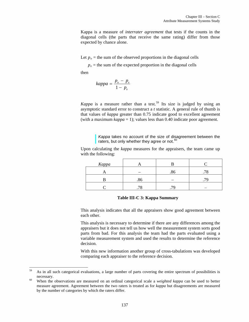
Chapter III – Section C Attribute Measurement Systems Study
137
Kappa is a measure of interrater agreement that tests if the counts in the diagonal cells (the parts that receive the same rating) differ from those expected by chance alone.
Let po = the sum of the observed proportions in the diagonal cells
pe = the sum of the expected proportion in the diagonal cells
then
1o e
e
p pkappa
p
Kappa is a measure rather than a test. P
59F Its size is judged by using an
asymptotic standard error to construct a t statistic. A general rule of thumb is that values of kappa greater than 0.75 indicate good to excellent agreement (with a maximum kappa = 1); values less than 0.40 indicate poor agreement.
Kappa takes no account of the size of disagreement between the raters, but only whether they agree or not. P
60F
Upon calculating the kappa measures for the appraisers, the team came up with the following:
Kappa A B C
A – .86 .78
B .86 – .79
C .78 .79 –
Table III-C 3: Kappa Summary
This analysis indicates that all the appraisers show good agreement between each other.
This analysis is necessary to determine if there are any differences among the appraisers but it does not tell us how well the measurement system sorts good parts from bad. For this analysis the team had the parts evaluated using a variable measurement system and used the results to determine the reference decision.
With this new information another group of cross-tabulations was developed comparing each appraiser to the reference decision.
59 As in all such categorical evaluations, a large number of parts covering the entire spectrum of possibilities is
necessary. 60 When the observations are measured on an ordinal categorical scale a weighted kappa can be used to better
measure agreement. Agreement between the two raters is treated as for kappa but disagreements are measured by the number of categories by which the raters differ.
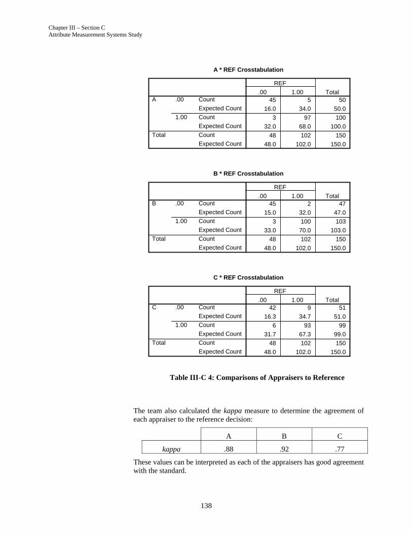
Chapter III – Section C Attribute Measurement Systems Study
138
Table III-C 4: Comparisons of Appraisers to Reference
The team also calculated the kappa measure to determine the agreement of each appraiser to the reference decision:
A B C
kappa .88 .92 .77
These values can be interpreted as each of the appraisers has good agreement with the standard.
A * REF Crosstabulation
45 5 50
16.0 34.0 50.0
3 97 100
32.0 68.0 100.0
48 102 150
48.0 102.0 150.0
Count
Expected Count
Count
Expected Count
Count
Expected Count
.00
1.00
A
Total
.00 1.00
REF
Total
B * REF Crosstabulation
45 2 47
15.0 32.0 47.0
3 100 103
33.0 70.0 103.0
48 102 150
48.0 102.0 150.0
Count
Expected Count
Count
Expected Count
Count
Expected Count
.00
1.00
B
Total
.00 1.00
REF
Total
C * REF Crosstabulation
42 9 51
16.3 34.7 51.0
6 93 99
31.7 67.3 99.0
48 102 150
48.0 102.0 150.0
Count
Expected Count
Count
Expected Count
Count
Expected Count
.00
1.00
C
Total
.00 1.00
REF
Total
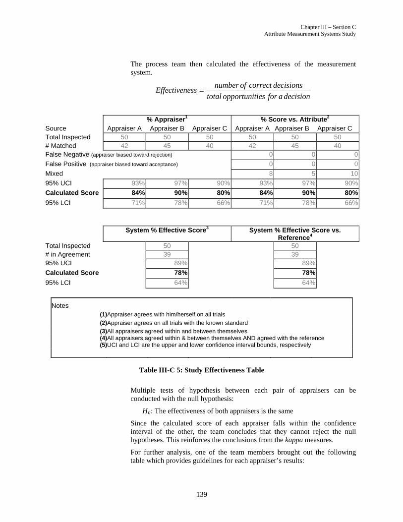
Chapter III – Section C Attribute Measurement Systems Study
139
The process team then calculated the effectiveness of the measurement system.
number of correct decisionsEffectiveness
total opportunities for a decision
% Appraiser1 % Score vs. Attribute2
Source Appraiser A Appraiser B Appraiser C Appraiser A Appraiser B Appraiser C Total Inspected 50 50 50 50 50 50 # Matched 42 45 40 42 45 40 False Negative (appraiser biased toward rejection) 0 0 0
False Positive (appraiser biased toward acceptance) 0 0 0
Mixed 8 5 10
95% UCI 93% 97% 90% 93% 97% 90%
Calculated Score 84% 90% 80% 84% 90% 80%
95% LCI 71% 78% 66% 71% 78% 66%
System % Effective Score3 System % Effective Score vs.
Reference4
Total Inspected 50 50 # in Agreement 39 39 95% UCI 89% 89%
Calculated Score 78% 78%
95% LCI 64% 64%
Notes (1)Appraiser agrees with him/herself on all trials (2)Appraiser agrees on all trials with the known standard (3)All appraisers agreed within and between themselves (4)(5)
All appraisers agreed within & between themselves AND agreed with the reference UCI and LCI are the upper and lower confidence interval bounds, respectively
Table III-C 5: Study Effectiveness Table
Multiple tests of hypothesis between each pair of appraisers can be conducted with the null hypothesis:
H0: The effectiveness of both appraisers is the same
Since the calculated score of each appraiser falls within the confidence interval of the other, the team concludes that they cannot reject the null hypotheses. This reinforces the conclusions from the kappa measures.
For further analysis, one of the team members brought out the following table which provides guidelines for each appraiser’s results:
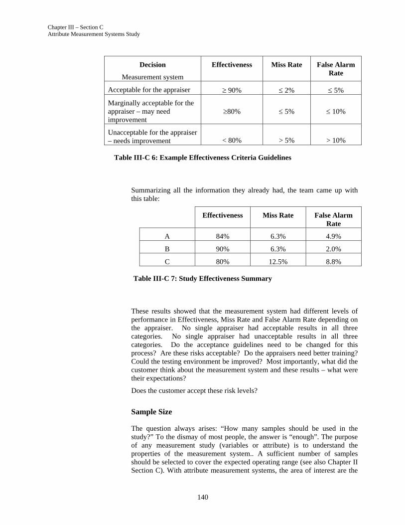
Chapter III – Section C Attribute Measurement Systems Study
140
Decision
Measurement system
Effectiveness Miss Rate False Alarm Rate
Acceptable for the appraiser 90% 2% 5%
Marginally acceptable for the appraiser – may need improvement
80% 5% 10%
Unacceptable for the appraiser – needs improvement < 80% > 5% > 10%
Table III-C 6: Example Effectiveness Criteria Guidelines
Summarizing all the information they already had, the team came up with this table:
Effectiveness Miss Rate False Alarm Rate
A 84% 6.3% 4.9%
B 90% 6.3% 2.0%
C 80% 12.5% 8.8%
Table III-C 7: Study Effectiveness Summary
These results showed that the measurement system had different levels of performance in Effectiveness, Miss Rate and False Alarm Rate depending on the appraiser. No single appraiser had acceptable results in all three categories. No single appraiser had unacceptable results in all three categories. Do the acceptance guidelines need to be changed for this process? Are these risks acceptable? Do the appraisers need better training? Could the testing environment be improved? Most importantly, what did the customer think about the measurement system and these results – what were their expectations?
Does the customer accept these risk levels?
Sample Size
The question always arises: “How many samples should be used in the study?” To the dismay of most people, the answer is “enough”. The purpose of any measurement study (variables or attribute) is to understand the properties of the measurement system.. A sufficient number of samples should be selected to cover the expected operating range (see also Chapter II Section C). With attribute measurement systems, the area of interest are the
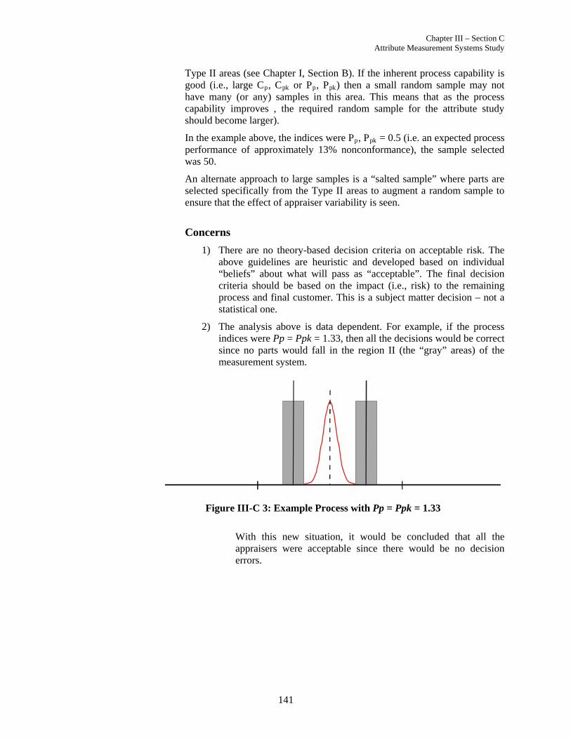
Chapter III – Section C Attribute Measurement Systems Study
141
Type II areas (see Chapter I, Section B). If the inherent process capability is good (i.e., large Cp, Cpk or Pp, Ppk) then a small random sample may not have many (or any) samples in this area. This means that as the process capability improves , the required random sample for the attribute study should become larger).
In the example above, the indices were Pp, Ppk = 0.5 (i.e. an expected process performance of approximately 13% nonconformance), the sample selected was 50.
An alternate approach to large samples is a “salted sample” where parts are selected specifically from the Type II areas to augment a random sample to ensure that the effect of appraiser variability is seen.
Concerns
1) There are no theory-based decision criteria on acceptable risk. The above guidelines are heuristic and developed based on individual “beliefs” about what will pass as “acceptable”. The final decision criteria should be based on the impact (i.e., risk) to the remaining process and final customer. This is a subject matter decision – not a statistical one.
2) The analysis above is data dependent. For example, if the process indices were Pp = Ppk = 1.33, then all the decisions would be correct since no parts would fall in the region II (the “gray” areas) of the measurement system.
Figure III-C 3: Example Process with Pp = Ppk = 1.33
With this new situation, it would be concluded that all the appraisers were acceptable since there would be no decision errors.
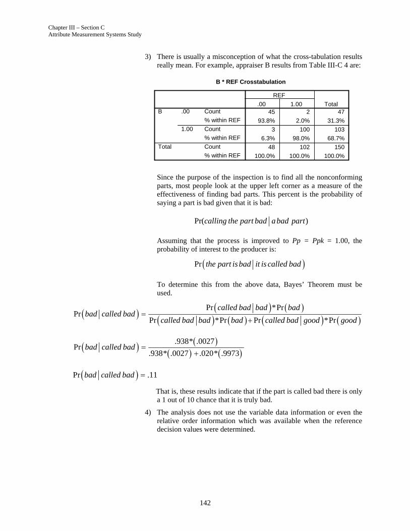
Chapter III – Section C Attribute Measurement Systems Study
142
3) There is usually a misconception of what the cross-tabulation results really mean. For example, appraiser B results from Table III-C 4 are:
Since the purpose of the inspection is to find all the nonconforming parts, most people look at the upper left corner as a measure of the effectiveness of finding bad parts. This percent is the probability of saying a part is bad given that it is bad:
Pr( )calling the part bad a bad part
Assuming that the process is improved to Pp = Ppk = 1.00, the probability of interest to the producer is:
Pr the part isbad it is called bad
To determine this from the above data, Bayes’ Theorem must be used.
Pr *PrPr
Pr *Pr Pr *Pr
called bad bad badbad called bad
called bad bad bad called bad good good
.938* .0027Pr
.938* .0027 .020* .9973bad called bad
Pr .11bad called bad
That is, these results indicate that if the part is called bad there is only a 1 out of 10 chance that it is truly bad.
4) The analysis does not use the variable data information or even the relative order information which was available when the reference decision values were determined.
B * REF Crosstabulation
45 2 47
93.8% 2.0% 31.3%
3 100 103
6.3% 98.0% 68.7%
48 102 150
100.0% 100.0% 100.0%
Count
% within REF
Count
% within REF
Count
% within REF
.00
1.00
B
Total
.00 1.00
REF
Total
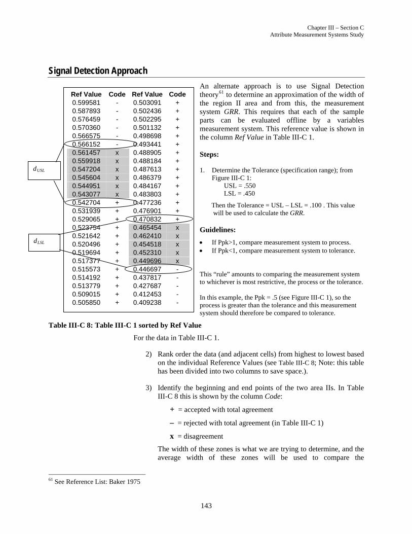
Chapter III – Section C Attribute Measurement Systems Study
143
Signal Detection Approach
An alternate approach is to use Signal Detection theory P
61F to determine an approximation of the width of
the region II area and from this, the measurement system GRR. This requires that each of the sample parts can be evaluated offline by a variables measurement system. This reference value is shown in the column Ref Value in Table III-C 1. Steps: 1. Determine the Tolerance (specification range); from
Figure III-C 1: USL = .550 LSL = .450
Then the Tolerance = USL – LSL = .100 . This value will be used to calculate the GRR. Guidelines:
If Ppk>1, compare measurement system to process. If Ppk<1, compare measurement system to tolerance.
This “rule” amounts to comparing the measurement system to whichever is most restrictive, the process or the tolerance. In this example, the Ppk = .5 (see Figure III-C 1), so the process is greater than the tolerance and this measurement system should therefore be compared to tolerance.
Table III-C 8: Table III-C 1 sorted by Ref Value
For the data in Table III-C 1.
2) Rank order the data (and adjacent cells) from highest to lowest based on the individual Reference Values (see Table III-C 8; Note: this table has been divided into two columns to save space.).
3) Identify the beginning and end points of the two area IIs. In Table III-C 8 this is shown by the column Code:
+ = accepted with total agreement
– = rejected with total agreement (in Table III-C 1)
x = disagreement
The width of these zones is what we are trying to determine, and the average width of these zones will be used to compare the
61 See Reference List: Baker 1975
Ref Value Code Ref Value Code0.599581 - 0.503091 + 0.587893 - 0.502436 + 0.576459 - 0.502295 + 0.570360 - 0.501132 + 0.566575 - 0.498698 + 0.566152 - 0.493441 + 0.561457 x 0.488905 + 0.559918 x 0.488184 + 0.547204 x 0.487613 + 0.545604 x 0.486379 + 0.544951 x 0.484167 + 0.543077 x 0.483803 + 0.542704 + 0.477236 + 0.531939 + 0.476901 + 0.529065 + 0.470832 + 0.523754 + 0.465454 x 0.521642 + 0.462410 x 0.520496 + 0.454518 x 0.519694 + 0.452310 x 0.517377 + 0.449696 x 0.515573 + 0.446697 - 0.514192 + 0.437817 - 0.513779 + 0.427687 - 0.509015 + 0.412453 - 0.505850 + 0.409238 -
dUSL
dLSL
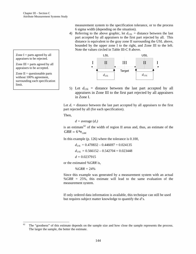
Chapter III – Section C Attribute Measurement Systems Study
144
measurement system to the specification tolerance, or to the process 6 sigma width (depending on the situation).
4) Referring to the above graphic, let dUSL = distance between the last part accepted by all appraisers to the first part rejected by all. This distance is equivalent to the gray zone II surrounding the USL above, bounded by the upper zone I to the right, and Zone III to the left. Note the values circled in Table III-C 8 above.
5) Let dLSL = distance between the last part accepted by all appraisers in Zone III to the first part rejected by all appraisers in Zone I.
Let di = distance between the last part accepted by all appraisers to the first part rejected by all (for each specification).
Then,
d = average (di)
is an estimate P
62F of the width of region II areas and, thus, an estimate of the
6*σ GRRGRR
In this example (p. 126) where the tolerance is 0.100,
dLSL = 0.470832 – 0.446697 = 0.024135
dUSL = 0.566152 – 0.542704 = 0.023448
d = 0.0237915
or the estimated %GRR is,
%GRR = 24%
Since this example was generated by a measurement system with an actual %GRR = 25%, this estimate will lead to the same evaluation of the measurement system.
If only ordered data information is available, this technique can still be used but requires subject matter knowledge to quantify the d’s.
62 The “goodness” of this estimate depends on the sample size and how close the sample represents the process.
The larger the sample, the better the estimate.
dUSL dLSL
Zone I = parts agreed by all appraisers to be rejected.
Zone III = parts agreed by all appraisers to be accepted.
Zone II = questionable parts without 100% agreement, surrounding each specification limit.
Chapter III – Section C Attribute Measurement Systems Study
145
Analytic Method P
63
As with any measurement system, the stability of the process should be verified and, if necessary, monitored. For attribute measurement systems, attribute control charting of a constant sample over time is a common way of verifying stability P
64F.
For an attribute measurement system, the concept of the Gage Performance Curve (see Chapter IV, Section F) is used for developing a measurement system study, which is used to assess the amount of repeatability and bias of the measurement system. This analysis can be used on both single and double limit measurement systems. For a double limit measurement system, only one limit need be examined with the assumptions of linearity and uniformity of error. For convenience, the lower limit will be used for discussion.
In general, the attribute measurement system study consists of obtaining the reference values for several selected parts. These parts are evaluated a number of times, (m), with the total number of accepts (a), for each part being recorded. From the results, repeatability and bias can be assessed.
The first stage of the attribute study is the part selection. It is essential that the reference value be known for each part used in the study. Eight parts should be selected at as nearly equidistant intervals as practical. The maximum and minimum values should represent the process range. Although this selection does not affect confidence in the results, it does affect the total number of parts needed to complete the gage study. The eight parts must be run through the gage, m = 20 times, and the number of accepts, (a), recorded.
For the total study, the smallest part must have the value a = 0; the largest part, a = 20; and the six other parts, a 19. If these criteria are not satisfied, more parts with known reference values, (X), must be run through the gage until the above conditions are met. If, for the smallest value a 0, then smaller and smaller parts are taken and evaluated until a = 0. If, for the largest value a 20, then larger and larger parts are taken until a = 20. If six of the parts do not have 1 a 19, additional parts can be taken at selected points throughout the range. These points are taken at the midpoints of the part measurements already measured in the study. The first interval at the a = 0 end starts from the largest measurement where a = 0. For the a = 20 end, the first interval starts at the smallest measurement where a = 20. For best results, samples should be taken at both the a = 0 and a = 20 ends and worked toward the middle of the part range. If necessary, the procedure can be repeated until the criteria are met.
Once the data collection criteria have been satisfied, the probabilities of acceptance must be calculated for each part using the following equations:
63 Adapted with permission from “Analysis of Attribute Gage Systems” by J. McCaslin & G. Gruska, ASQC,
1976. 64 Caveat: np > 4
Chapter III – Section C Attribute Measurement Systems Study
146
5.05.0
205.05.0
0,5.05.0
'
m
aif
am
aif
m
a
am
aif
m
a
Pa
The adjustments cover the instances where 1 a 19. For the instances where a = 0 set aP = 0 except for the largest reference value with a = 0, in
which aP = 0.025. For the instances where a = 20 then aP = 1 except for the
smallest reference value with a = 20 in which aP = 0.975.
Once the aP has been calculated for each XT , the Gage Performance Curve
(GPC) can be developed. Although the GPC can be presented graphically (see Figure III-C 5), use of normal probability paper (see Figure III-C 4) yields more accurate estimates of the repeatability and bias.
The calculated probabilities are plotted on normal probability paper and a line of best fit is drawn through these points. The bias is equal to the lower limit minus the reference value measurement that corresponds to aP = 0.5,
or
bias = Lower Specification Limit – XT (at aP = 0.5)
The repeatability is determined by finding the differences of the reference value measurements corresponding aP = 0.995 and aP =0.005 and dividing
by an adjustment factor of 1.08 P
65F.
1.08
' 'T a T aX (at P 0.995) X ( at P 0.005)
Repeatability
To determine if the bias is significantly different from zero, the following statistic is used:
repeatability
6.078 Biast
If this calculated value is greater than 2.093 (t025,19), then the bias is significantly different from zero.
An example will clarify the attribute study data collection and calculation of repeatability and bias.
65 The 1.08 adjustment (unbiasing) factor is specific for a sample size of 20 and was determined through a
simulation of this approach with a 99% repeatability range. To convert the result to a 6 sigma range, divide by 5.15 and multiply by 6.
Chapter III – Section C Attribute Measurement Systems Study
147
Example: An attribute gage is being used to measure a dimension that has a tolerance of 0.010. The gage is an end-of-line 100% automatic inspection gage that is affected by repeatability and bias. To perform the attribute study, eight parts with reference values at intervals of 0.002 from –0.016 to –0.002 are run through the gage 20 times each. The number of accepts for each part are:
XT a
–0.016 0 –0.014 3 –0.012 8 –0.010 20 –0.008 20 –0.006 20 –0.004 20 -0.002 20
Since there are two reference values with 1 a 19, at least four more parts must be found. Therefore, it is necessary to run parts with reference values at the midpoints of the existing intervals. These reference values and the number of accepts are:
–0.015 1 –0.013 5 -0.011 16
Now there are five reference values with 1 a 19. The procedure requires that one more part be found with 1 a 19. Therefore, the following part is evaluated:
–0.0105 18
Now that the data collection criteria have been satisfied, the probabilities of acceptance can be calculated using the binomial adjustments shown below.
XT a
aP
-0.016 0 0.025 -0.015 1 0.075 -0.014 3 0.175 -0.013 5 0.275 -0.012 8 0.425 -0.011 16 0.775
-0.0105 18 0.875 -0.010 20 0.975 -0.008 20 1.000
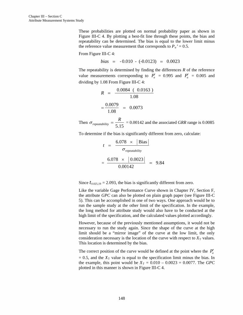
Chapter III – Section C Attribute Measurement Systems Study
148
These probabilities are plotted on normal probability paper as shown in Figure III-C 4. By plotting a best-fit line through these points, the bias and repeatability can be determined. The bias is equal to the lower limit minus the reference value measurement that corresponds to Pa’ = 0.5.
From Figure III-C 4:
- 0.010 - (-0.0123) 0.0023bias
The repeatability is determined by finding the differences R of the reference value measurements corresponding to aP = 0.995 and aP = 0.005 and
dividing by 1.08 From Figure III-C 4:
0.0084 ( 0.0163 )
1.08R
0.0079
0.00731.08
Then 5.15
repeatabilityR
= 0.00142 and the associated GRR range is 0.0085
To determine if the bias is significantly different from zero, calculate:
6.078 Bias
repeatability
t
= 6.078 0.0023
9.840.00142
Since t0.025,19 = 2.093, the bias is significantly different from zero.
Like the variable Gage Performance Curve shown in Chapter IV, Section F, the attribute GPC can also be plotted on plain graph paper (see Figure III-C 5). This can be accomplished in one of two ways. One approach would be to run the sample study at the other limit of the specification. In the example, the long method for attribute study would also have to be conducted at the high limit of the specification, and the calculated values plotted accordingly.
However, because of the previously mentioned assumptions, it would not be necessary to run the study again. Since the shape of the curve at the high limit should be a “mirror image” of the curve at the low limit, the only consideration necessary is the location of the curve with respect to XT values. This location is determined by the bias.
The correct position of the curve would be defined at the point where the aP = 0.5, and the XT value is equal to the specification limit minus the bias. In the example, this point would be XT = 0.010 – 0.0023 = 0.0077. The GPC plotted in this manner is shown in Figure III-C 4.
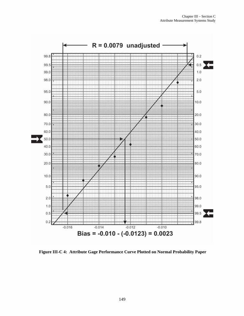
Chapter III – Section C Attribute Measurement Systems Study
149
Figure III-C 4: Attribute Gage Performance Curve Plotted on Normal Probability Paper
Chapter III – Section C Attribute Measurement Systems Study
150
Figure III-C 5. Attribute Gage Performance Curve
Chapter IV Other Measurement Concepts and Practices
151
CHAPTER IV
Other Measurement Concepts and Practices

Chapter IV Other Measurement Concepts and Practices
152
Chapter IV – Section A Practices for Complex or Non-Replicable Measurement Systems
153
Section A Practices for Non-Replicable Measurement Systems
The focus of this reference manual is measurement systems where the readings can be replicated for each part. Not all measurement systems have this characteristic; for example:
Destructive measurement systems Systems where the part changes on use/test.
The following are examples of approaches to the analysis of measurement systems, including those not previously discussed in this manual. This is not intended to be a complete listing covering every type of measurement system but only examples of various approaches. If a measurement system does not fit the manual’s focus, it is recommended that assistance from competent statistical resources be consulted.
Destructive measurement systems
When the part (characteristic) being measured is destroyed by the act of measuring the process is known as destructive measurement. This includes the whole class of measurement systems known as “destructive measurement systems”; for example destructive weld testing, destructive plating testing, salt spray/humidity booth testing, impact testing (gravelometer) or mass spectroscopy and other material characteristic testing processes. These are the “classic” examples of a non-replicable measurement system since repeated readings cannot be taken on any single part.
Systems where the part changes on use/test
However, there are other measurement systems which are non-replicable where the part, itself, is not harmed by the measurement process but the characteristic being measure will change. Examples of this are: leak tests with qualitative data, testing using engine test stands, transmission test stands, vehicle dynamometers, etc. Analysis of these systems will depend on whether
1) A homogeneous set of parts (small between part variation) can be found to represent a single part;
2) The shelf life of the characteristic (property) is known and extends beyond the expected duration of the study – i.e., the measured characteristic does not change over the expected period of use; or
3) The dynamic (changing) properties can be stabilized
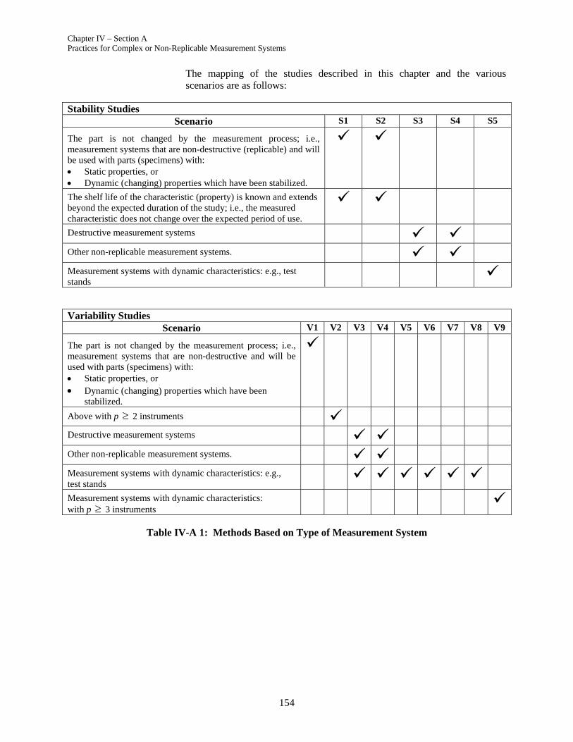
Chapter IV – Section A Practices for Complex or Non-Replicable Measurement Systems
154
The mapping of the studies described in this chapter and the various scenarios are as follows:
Stability Studies Scenario S1 S2 S3 S4 S5
The part is not changed by the measurement process; i.e., measurement systems that are non-destructive (replicable) and will be used with parts (specimens) with: Static properties, or Dynamic (changing) properties which have been stabilized.
The shelf life of the characteristic (property) is known and extends beyond the expected duration of the study; i.e., the measured characteristic does not change over the expected period of use.
Destructive measurement systems
Other non-replicable measurement systems.
Measurement systems with dynamic characteristics: e.g., test stands
Variability Studies
Scenario V1 V2 V3 V4 V5 V6 V7 V8 V9
The part is not changed by the measurement process; i.e., measurement systems that are non-destructive and will be used with parts (specimens) with: Static properties, or Dynamic (changing) properties which have been
stabilized.
Above with p 2 instruments
Destructive measurement systems
Other non-replicable measurement systems.
Measurement systems with dynamic characteristics: e.g., test stands
Measurement systems with dynamic characteristics: with p 3 instruments
Table IV-A 1: Methods Based on Type of Measurement System
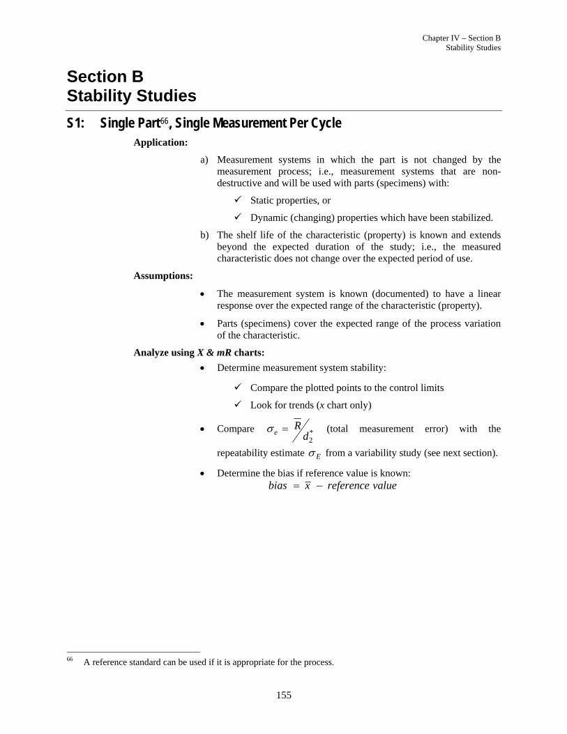
Chapter IV – Section B Stability Studies
155
Section B Stability Studies
S1: Single Part P
66F, Single Measurement Per Cycle
Application:
a) Measurement systems in which the part is not changed by the measurement process; i.e., measurement systems that are non-destructive and will be used with parts (specimens) with:
Static properties, or
Dynamic (changing) properties which have been stabilized.
b) The shelf life of the characteristic (property) is known and extends beyond the expected duration of the study; i.e., the measured characteristic does not change over the expected period of use.
Assumptions:
The measurement system is known (documented) to have a linear response over the expected range of the characteristic (property).
Parts (specimens) cover the expected range of the process variation of the characteristic.
Analyze using X & mR charts:
Determine measurement system stability:
Compare the plotted points to the control limits
Look for trends (x chart only)
Compare *2
eR
d (total measurement error) with the
repeatability estimate E from a variability study (see next section).
Determine the bias if reference value is known: bias x reference value
66 A reference standard can be used if it is appropriate for the process.
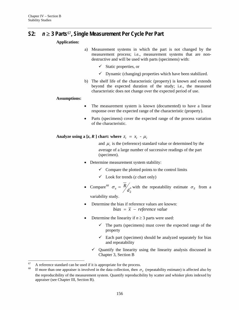
Chapter IV – Section B Stability Studies
156
S2: n 3 Parts P
67F, Single Measurement Per Cycle Per Part
Application:
a) Measurement systems in which the part is not changed by the measurement process; i.e., measurement systems that are non-destructive and will be used with parts (specimens) with:
Static properties, or
Dynamic (changing) properties which have been stabilized.
b) The shelf life of the characteristic (property) is known and extends beyond the expected duration of the study; i.e., the measured characteristic does not change over the expected period of use.
Assumptions:
The measurement system is known (documented) to have a linear response over the expected range of the characteristic (property).
Parts (specimens) cover the expected range of the process variation of the characteristic.
Analyze using a [z, R ] chart: where - i i iz x
and i is the (reference) standard value or determined by the
average of a large number of successive readings of the part (specimen).
Determine measurement system stability:
Compare the plotted points to the control limits
Look for trends (z chart only)
Compare P
68F e *
2
Rd
with the repeatability estimate E from a
variability study.
Determine the bias if reference values are known: bias x reference value
Determine the linearity if n 3 parts were used:
The parts (specimens) must cover the expected range of the property
Each part (specimen) should be analyzed separately for bias and repeatability
Quantify the linearity using the linearity analysis discussed in Chapter 3, Section B
67 A reference standard can be used if it is appropriate for the process. 68 If more than one appraiser is involved in the data collection, then E (repeatability estimate) is affected also by
the reproducibility of the measurement system. Quantify reproducibility by scatter and whisker plots indexed by appraiser (see Chapter III, Section B).
Chapter IV – Section B Stability Studies
157
If more than one instrument is use in this study, determine consistency (homogeneity of variation) among the instruments; e.g., use F test, Bartlett’s test, Levene’s test P
69F, etc.
S3: Large Sample from a Stable Process Application:
The measurement system must be evaluating a homogeneous independent identically distributed (“iid”) sample (collected and isolated). The measurements of individual parts (specimens) are not replicated so this study can be used with destructive and non-replicable measurement systems.
Assumptions:
The shelf life of the characteristic (property) is known and extends beyond the expected duration of the study; i.e., measured characteristic does not change over the expected period of use and/or storage.
Parts (specimens) cover the expected range of the process variation of the characteristic (property).
The measurement system’s linearity is known (documented) over the expected range of the characteristic (property). (If the response is non-linear, the readings must be adjusted accordingly.)
Analyze by:
Determining the total variability via a capability study with n 30 parts. (This preliminary study should also be used to verify the consistency of the sample: i.e., all parts (specimens) come from a unimodal distribution.)
2 2 2total process measurement system
Measuring one or more individuals from the isolated sample per time period, use x & R or x & mR charts with the control limits determined by the capability study.
Compare the plotted points to the control limits.
Look for trends.
Since the parts (specimens) do not change (an isolated sample), any indication of instability would be attributed to a change in the measurement system.
69 Dataplot, National Institute of Standards and Technology, Statistical Engineering Division (www.itl.nist.gov).

Chapter IV – Section B Stability Studies
158
S4: Split Specimens (General), Single Specimen Per Cycle Application:
The measurements of individual parts (specimens) portions are not replicated so this study can be used with destructive and non-replicable measurement systems.
Assumptions:
The shelf life of the characteristic (property) is known and extends beyond the expected duration of the study; i.e., measured characteristic does not change over the expected period of use and/or storage.
Parts (specimens) cover the extended range of the process variation of the characteristic (property).
Specimens are split into m portions. With m=2 portions, this is often called a test-retest study.
Analyze using:
Range chart to track the consistency of the measurements (confounded with the “within-lot” consistency).
Compare *2
eR
d with the repeatability estimate E from a
variability study.
This is an upper bound study: 2 2 2 = + e E btwn
Chart to track the consistency of the production process.
S4 with Pairs of Consecutive (Homogeneous) Parts from Different Lots – S4a
This study is the same as S4 with homogeneous parts from different lots. It is
an upper bound study, since 2 2 2 2 e E btwn lots
Chapter IV – Section B Stability Studies
159
S5: Test Stands
In this situation, multiple measurement instruments (test stands) evaluate the same characteristics of a continual stream of product. The product stream is randomly assigned to individual stands.
S5a: Attribute Responses Analyze using p charts:
Determine consistency (of decisions) among the stands: a single chart including the results from all the stands.
Determine stability within individual stands: separate chart for each stand.
Analyze the total system stability with a p & mR chart where p is the average over all the test stands in a given day.
S5b: Variable Data Responses Analyze using ANOVA and graphical techniques: P
70
Calculate x & s for each test stand (by characteristic), by time period.
Determine consistency among the stands: a single x & s chart including the results from all the stands.
Determine stability within individual stands: separate x & s chart for each stand.
Quantify the consistency (homogeneity of variation) among the stands; e.g., use F test, Bartlett’s test, Levene’s test, etc.
Determine if all stands are on the same target by comparing stand averages; e.g., using a one-way ANOVA analysis. If any difference exists, isolate different stands by using, for example, Tukey’s T test.
70 see also James, P. D., “Graphical Displays of Gage R&R Data,” AQC Transaction, ASQC, 1991

Chapter IV – Section B Stability Studies
160
Chapter IV – Section C Variability Studies
161
Section C Variability Studies
All descriptive studies are enumerative in nature in that they describe the measurement system (including the effects of the environment) during the study. Since measurement systems are to be used in making future decisions about products, processes, or services, an analytic conclusion about the measurement system is necessary. The transition from enumerative to analytic results requires subject matter knowledge and expertise to:
Assure that all expected measurement sources of variation are considered in the design and execution of the study.
Analyze the results (data) in light of the expected uses, environment, control, maintenance, etc.
V1: Standard GRR Studies
These studies are those contained within this reference manual. These studies include graphical analysis as well as numerical analysis.
V1a – Range Method (R&R)
V1b – Range Method (R&R and Within-Part)
V1c – ANOVA Method
V1d – Modified ANOVA/Range Method
V2: Multiple Readings With p 2 Instruments
This allows the comparison of multiple instruments. Application:
a) Measurement systems in which the part is not changed by the measurement process; i.e., measurement systems that are non-destructive and will be used with parts (specimens) with:
1) Static properties, or
2) Dynamic (changing) properties which have been stabilized.
Assumptions:
The shelf life of the characteristic (property) is known and extends beyond the expected duration of the study; i.e., the measured characteristic does not change over the expected period of use.
Parts (specimens) cover the expected range of the process variation of the characteristic.

Chapter IV – Section C Variability Studies
162
Analyze using Grubbs’ P
71F (or Thompson’s) P
72F estimates:
Process variability
Instrument variability = repeatability
Confidence region calculations are available
V3: Split specimens (m = 2) Application:
The measurements of individual parts (specimens) portions are not replicated so this study can be used with destructive and non-replicable measurement systems and can be used to analyze measurement systems with dynamic characteristics.
Assumptions:
The shelf life of the characteristic (property) is known and extends beyond the expected duration of the study; i.e., measured characteristic does not change over the expected period of use and/or storage.
Parts (specimens) cover the extended range of the process variation of the characteristic (property).
Specimens are split into m portions. With m=2 portions, this is often called a test-retest study.
Analyze using regression techniques:
Estimate repeatability with the error term: eE
Linearity (by comparing estimated line with 45° line)
V3a – V3 with Pairs of Consecutive Parts
This study is the same as V3 using consecutive pairs of part rather than split specimens. This study is used in situations where the part cannot be split without destroying the property to be measured.
This is an upper bound study: E e btwn
71 See Reference List, Grubbs, F. E., 1973. 72 See Reference List, Thompson, W. A., Jr., 1963.

Chapter IV – Section C Variability Studies
163
V4: Split Specimens (General) Application:
The measurements of individual parts (specimens) portions are not replicated so this study can be used with destructive and non-replicable measurement systems and can be used to analyze measurement systems with dynamic characteristics.
Assumptions:
The shelf life of the characteristic (property) is known and extends beyond the expected duration of the study; i.e., measured characteristic does not change over the expected period of use and/or storage.
Parts (specimens) cover the extended range of the process variation of the characteristic (property).
Split specimens into m portions where m = 0 mod 2 or 3; m 2 (e.g., m =3, 4, 6, 9,.....).
Analyze using:
Standard GRR techniques including graphics
ANOVA – Randomized Block Design (two-way ANOVA)
V4a – V4 with Pairs of Consecutive (homogeneous) Parts from Different Lots
This study is the same as V4 using consecutive pairs of part rather than split specimens. This study is used in situations where the part cannot be split without destroying the property to be measured.
This is an upper bound study: E e parts lots
The Following Studies Assume the Part (specimen) Characteristic (property) is Dynamic.
V5: Same as V1 with Stabilized Parts
The parts used in the study are stabilized using a process based on engineering knowledge and expertise; e.g., engines which are ‘broken-in’ versus ‘green’ engines.
Chapter IV – Section C Variability Studies
164
V6: Time Series Analysis
Assumptions:
Repeated readings are taken over specified time intervals .
The shelf life of the characteristic (property) is known and extends beyond the expected duration of the study; i.e., the measured characteristic does not change over the expected period of use.
Parts (specimens) cover the expected range of the process variation of the characteristic.
Analyze by determining the degradation model for each sample part:
eE
Consistency of degradation (if n 2)
V7: Linear Analysis
Assumptions:
Repeated readings are taken over specified time intervals.
The degradation in the measurement system is known (documented) to have a linear response over the specified time intervals.
The shelf life of the characteristic (property) is known and extends beyond the expected duration of the study; i.e., the measured characteristic does not change over the expected period of use.
Parts (specimens) cover the expected range of the process variation of the characteristic.
Analyze by linear regression:
eE
Consistency of degradation (if n 2)
V7a – V7 with a Homogeneous Sample
Analyze by linear regression:
This is an upper bound study: E e btwn
V8: Time versus Characteristic (Property) Degradation
V6 & V7 can be modified to determine if the degradation is time (i.e., shelf life) or activity dependent.

Chapter IV – Section C Variability Studies
165
V9: V2 with Simultaneous Multiple Readings and p 3 Instruments
Analyze same as V2 (see also Lipson & Sheth, sec 13.2).

Chapter IV – Section C Variability Studies
166

Chapter IV – Section D Quantifying the Effect of Excessive Within-Part Variation
167
Section D Recognizing the Effect of Excessive Within-Part Variation
Understanding the sources of variation of a measurement system is important for all measurement applications but becomes even more critical where there is significant within-part variation. Within-part variation, such as taper or out-of-round, can cause the measurement system evaluation to provide misleading results. This is because unaccounted within-part variation affects the estimate of repeatability, reproducibility, or both. That is, the within-part variation can appear as a significant component of the measurement system variation. Understanding the within-part variation present in the product will result in a more meaningful understanding of the suitability of the measurement system for the task at hand.
Examples of within-part variation which may be encountered are: roundness (circular runout), concentricity, taper, flatness, profile, cylindricity, etc. P
73F It
is possible that more than one of these characteristics may be present at the same time within the same part (composite error). The strength of each characteristic and their interdependencies may compound the data and the resultant understanding of the measurement system. Recognition and analysis of these additional sources of variation during a measurement system study is paramount to understanding the actual measurement system variation. A D.O.E., ANOVA or other more sophisticated statistical technique may be required to analyze this situation. Whatever methodology is chosen should be approved by the customer supplier quality representative.
Also, decisions that product design engineers make can unwittingly affect how a part is measured, how a fixture may be designed, and the result can affect the outcome of measurement error. An example might be a plastic part that has a critical feature on the parting line (a parting line typically has excess plastic material where the two halves of the mold join, and thus is an uncontrolled surface). These factors ought to be considered during a Design FMEA.
73 Many of these features are controlled in the design by way of Geometric Dimensioning and Tolerancing (GD&T). GD&T provides an operationally defined method to check parts in a functional manner. Generally, a functional check is an attribute check. Where variable data is required, issues can arise as to using a gage designed for a functional check to yield variable data. This may sometimes be done by using the functional gage as a holding fixture for a CMM study. However, when this is done it is critical that the fixture hold the part firmly and repeatably in the same location (if it does not, the resultant MSA study should generate this error).

Chapter IV – Section D Quantifying the Effect of Excessive Within-Part Variation
168
Once the within-part variation components are understood, it may be possible to control these factors within the measurement system (e.g., by redesigning the gage or using different fixturing methods/equipment) so that future data is not confounded.
Chapter IV – Section E Average and Range Method – Additional Treatment
169
Section E Average and Range Method – Additional Treatment
There is an additional consideration worthy of mention relative to the Average and Range method of measurement system assessment. P
74F
The primary purpose of this graphical approach is the same as other well designed measurement system analyses: to determine if the measurement process is adequate to measure the manufacturing process variation and/or evaluate product conformance
Are all gages doing the same job?
Are all appraisers doing the same job?
Is the measurement system variation acceptable with respect to the process variation?
How good are the data obtained from the measurement process or into how many non-overlapping groups or categories can the data be divided?
1) Care should be taken to follow the “Preparation for Measurement
Systems Study”, Chapter II, Section C.
2) Have each appraiser check each sample for the characteristic being studied. Record the first checks on the top data row of a control chart (see Figure IV-E 1 & 2).
3) Repeat the checks and record the data on the second data row of the control chart. (Note: Do not allow the appraisers to see their original reading while making this second check.) The data should now show two checks on the same part by each appraiser.
4) Analyze the data by calculating the average ( X ) and range (R) for each subgroup.
5) Plot the range values on the range chart and calculate the average
range ( R ) (include all sub-group ranges (R) for all appraisers). Draw this average range on the chart. Use the D4 factor for n = 2 to calculate the control limit for the range chart. Draw in this limit and determine if all values are in control.
If all ranges are in control, all appraisers are doing the same job.If one appraiser is out of control, his method differs from the others.
If all appraisers have some out-of-control ranges, the measurement system is sensitive to appraiser technique and needs improvement to obtain useful data.
74 The control chart example is taken with permission from “Evaluating the Measurement Process,” by Wheeler &
Lyday (see Reference List).
Procedural Steps
Chapter IV – Section E Average and Range Method – Additional Treatment
170
6) Next, plot the average for each subgroup ( X ) for all appraisers on the average chart (see Figure IV-E 1 & 2). The average values represent both variation and measurement variation.
Calculate the grand average ( X ) (include all subgroup averages ( X ) for all
appraisers). Draw this grand average ( X ) on the chart.
Now calculate the control limits for this chart using the A2 factor for n = 2
and average range ( R ) from the range chart and draw these limits on the average chart. Note in this study, the range chart contains only measurement variation. Thus, the area between the control limits of the averages represents the amount of measurement variation in the system.
If all averages fall inside the control limits, the measurement variation overshadows the process variation. In other words, the measurement process has more variation than the manufacturing process and is of no value in monitoring or controlling that process.
If less than half of the averages are outside the limits, the measurement system is inadequate for process control.
On the other hand, if a majority of the averages fall outside the control limits, it indicates that the signals from the manufacturing process are greater than measurement variation. This measurement system can provide useful data for controlling the process.
Worksheet Example The question, “How good are the data collected by this measurement system?” can be answered by completing the worksheet example, Figure IV-E 3 & 4. All data needed for the worksheet can be found on the average and range charts described above.
Following are the steps used in completing the worksheet example (Figure IV-E 3 & 4):
1) Identify the measurement and characteristic being evaluated, who is doing the study and the date of the study.
2) The average subgroup range ( R ) is obtained directly from the control chart.
3) The number of replications (r) is the number of times each appraiser checked the same part.
4) Calculate the estimated repeatability standard deviation ( ˆe ), as
shown in Figure IV-E 3 by using the 2d value for the corresponding r.
5) Insert the number of appraisers (nA ) in the space provided.
6) Insert the number of samples (n) in the space provided.
Chapter IV – Section E Average and Range Method – Additional Treatment
171
7) Compute each appraiser average by averaging all the samples obtained by each appraiser and enter these averages in the space provided for each appraiser (A, B, C).
8) Examine the appraiser averages (A, B, C) and determine the range of the appraiser averages by subtracting the lowest from the highest and insert in the space for (RA).
9) Compute the estimated appraiser standard deviation ( ˆ A ) as shown
by using the *2d value for the corresponding nA value.
10) Compute the sample averages by averaging the value obtained by all appraisers for each sample. For example, (sample 1 avg. of appraiser A + sample 1 avg. of appraiser B + sample 1 avg. of the last appraiser and divide this sum by the number of appraisers). This is the best estimate of that sample’s true value. Place the value for each sample in the space provided (1, 2, 3.....9, 10) in Figure IV-E 4.
11) Observe the sample averages (1, 2, 3......9, 10) and calculate the range of the sample averages ( PR ) by subtracting the lowest from the highest. Insert this value in the space provided.
12) Estimate the sample-to-sample standard deviation ˆ( )P as shown by
using the *2d value for the corresponding n value.
13) Compute the “Signal-to-Noise Ratio” (SN) by dividing the sample standard deviation by the measurement standard deviation and insert in the space provided.
P
GRR
SN
14) Determine the number of distinct product categories that can be distinguished by these measurements. Multiply SN by 1.41 and insert in the space provided (Figure IV-E 4).
Only the integer portion of this number need be considered since it is defining distinct categories. (Drop all decimal fractions.) (See Figure IV-E 4.)
If the number of categories is less than two (2), the measurement system is of no value in controlling the process. It is all noise and one part cannot be said to be different from another.
If the number of categories is two (2), it means the data can be divided into only high and low groups; however this is only the equivalent of attribute data.
If the number of categories is three (3), the data can be divided into high, medium and low groups. This is a slightly better measurement system.
A system containing four (4) or more categories would be much better than the first three examples.
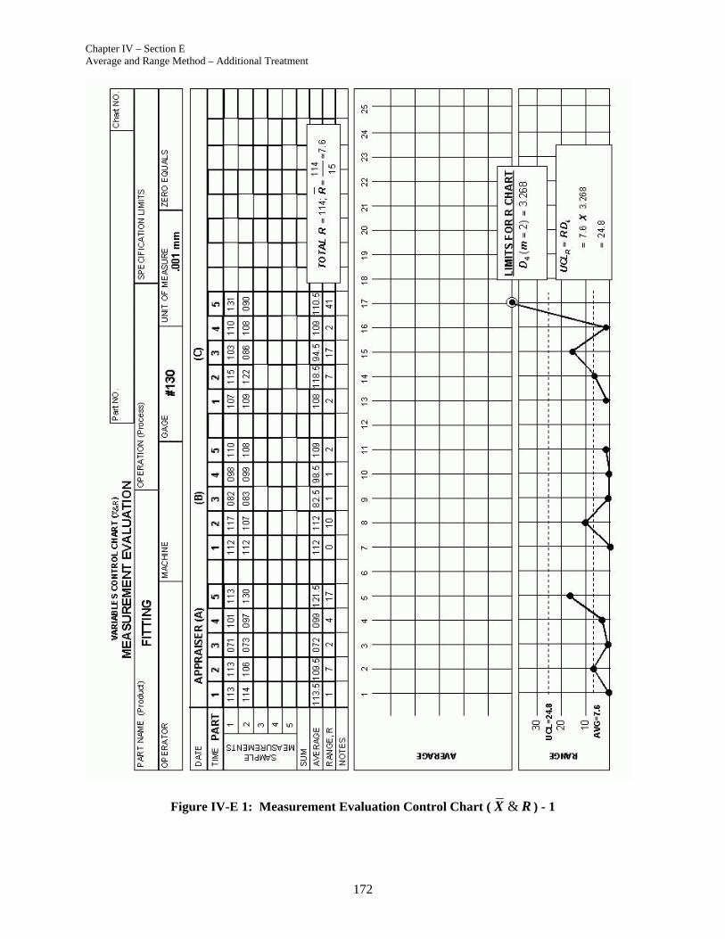
Chapter IV – Section E Average and Range Method – Additional Treatment
172
Figure IV-E 1: Measurement Evaluation Control Chart ( &X R ) - 1
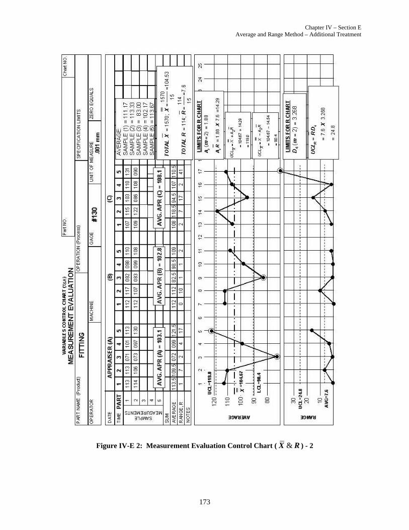
Chapter IV – Section E Average and Range Method – Additional Treatment
173
Figure IV-E 2: Measurement Evaluation Control Chart ( &X R ) - 2

Chapter IV – Section E Average and Range Method – Additional Treatment
174
Measurement Done Evaluated______FITTING LENGTH____ By_____R.W.L._____ Date__MM-DD-YY____
REPLICATION ERROR: Average Subgroup Range 7.6R Number of Replications = Subgroup Size = r = 2
Estimate Replication Standard Deviation
2
ˆ 6.738e
R
d
CALCULATIONS FOR APPRAISER EFFECT: Write appraiser averages below: Appraiser Average
Number of Appraisers 3A
n A 103.1
B – lo 102.8
Number of Samples 5n C – hi 108.1
108.1-102.8 AR D ____
Range of Appraiser Averages 5.3AR E ____
F ____
5.3
ˆ1.906
A
*2
ˆ 2.781A
R
d
Figure IV-E 3: Alternate Computations for Evaluating a Measurement Process (Part 1 of 2).
2 1.410
3 1.906
4 2.237
5 2.477
6 2.669
7 2.827
8 2.961
9 3.076
10 3.178
nA *2d
r
2 1.128
3 1.693
4 2.059
5 2.326
6 2.534
7 2.704
8 2.847
9 2.970
10 3.078
2
d

Chapter IV – Section E Average and Range Method – Additional Treatment
175
CALCULATIONS FOR MEASUREMENT ERROR STANDARD DEVIATION: Estimate the measurement error standard deviation to be:
2 2
2 2
ˆ ˆ ˆ
= (6.7376) + (2.7806)
= 7.289
m e A
Write the appropriate value for ˆm here: ˆ 7.289
m
CALCULATIONS FOR SIGNAL TO NOISE RATIO:
Write the average for each sample piece or batch below: Sample Average
113.67 - 83.0 p
R
Range for these Sample Averages 30.67p
R
Estimate Sample to Sample Standard Deviation:
30.67
12.382.477
*2
ˆ 12.38P
Pd
R
Signal to Noise Ratio:
12.38
1.6987.289
ˆ
1.698ˆ
P
m
Thus the number of distinct product categories that can be Reliably distinguished by these measurements is 1.41 x 1.698
ˆ
1.41 2.395ˆ
P
m
or 2
This is the number of non-overlapping 97% confidence intervals that will span the range of product variation. (A 97% confidence interval centered on a single measurement would contain the actual product value that is represented by that measurement 97% of the time.)
Figure IV-E 4: Alternate Computations for Evaluating a Measurement Process (Part 2 of 2).
2 1.410
3 1.906
4 2.237
5 2.477
6 2.669
7 2.827
8 2.961
9 3.076
10 3.178
n *2d
2 113.33
3 - Lo 83.00
4 102.17
5 - Hi 113.67
6
7
8
9
10
1 111.17

Chapter IV – Section E Average and Range Method – Additional Treatment
176
Chapter IV – Section F Gage Performance Curve
177
Section F Gage Performance Curve P
75
The purpose of developing a Gage Performance Curve (GPC) is to determine the probability of either accepting or rejecting a part of some reference value. Ideally, the GPC for a measurement without error is shown in Figure IV-F 1. However, this is the ideal for measurement systems, rather than what normally occurs.
Once the amount of error has been determined, it is possible to calculate the probability of accepting a part of some reference value when using that system.
To accomplish this, the assumption is made that the measurement system error consists primarily of lack of repeatability, reproducibility and bias. Further, repeatability and reproducibility are taken to be normally distributed with some variance, 2 . Consequently, gage error is normally distributed with a mean XT, the reference value, plus the bias, and has some variance,
2 . In other words:
2, )( T bActual Value from the Gage N X
The probability of accepting a part of some reference value is given by the relationship
2 ( , ) UL
a TLL
P N X b dx
Using the standard normal table
- ( ) - ( ) - T T
aUL X b LL X b
P
where
2 - ( )( , )
ULT
TUL X b
N X b dx
2 - ( )( , ) T
TLL
LL X bN X b dx
75 Adapted with permission from “Analysis of Attribute Gage Systems” by J. McCaslin & G. Gruska, ASQC,
1976.
Chapter IV – Section F Gage Performance Curve
178
Example: Determine the probability of accepting a part when the reference torque value is 0.5 Nm, 0.7 Nm, 0.9 Nm.
Using data from a previously conducted study:
Upper specification = USL = 1.0 Nm
Lower specification = LSL = 0.6 Nm
bias = b = 0.05 Nm
GRR = 0.05 Nm
Applying the above to the formulas on the previous page:
- ( ) - ( ) - T T
aUL X b LL X b
P
1.0 - (0.5 0.05) 0.6 - (0.5 0.05) -
0.05 0.05aP
(9.0) (1.0)aP
= 1.0 – 0.84
= 0.16
That is, when the part has a reference value of 0.5 Nm it will be rejected approximately 84% of the time.
Gage Performance Curve Example: For XT = 0.7 Nm
1.0 - (0.7 0.05) 0.6 - (0.7 0.05) -
0.05 0.05aP
(5.0) ( 3.0)aP
= 0.999
If the reference value of the part is 0.7 Nm then it will be rejected less than approximately 0.1% of the time.
For XT = 0.9 Nm
1.0 - (0.9 0.05) 0.6 - (0.9 0.05) -
0.05 0.05aP
(1.0) ( 7.0)aP
= 0.84
Chapter IV – Section F Gage Performance Curve
179
If the reference value of the part is 0.9 Nm then it will be rejected approximately less than 16% of the time.
If the probability of acceptance is calculated for all values of XT and plotted, then the Gage Performance Curve, as shown in Figure IV-F 2, would be obtained.
This same curve can be more easily plotted on normal probability paper, as shown in Figure IV-F 3. Once plotted, the GPC gives the probability of accepting a part of any part size.
In addition, once GPC is developed, it can be used to calculate the repeatability and reproducibility error, and the bias error P
76F.
The 6 GRR range can be determined by finding the XT value that corresponds to Pa = 0.99865 (z = 3), and the XT value that corresponds to Pa = 0.00135 (z = -3) for either of the two limits. The GRR is the difference between the two XT values, as shown graphically in Figure IV-F 3.
An estimate of the bias is determined by finding the XT, for either the upper or lower limit, that corresponds to Pa = 0.5, and calculating:
B = XT – LSL or BB = XT – USL
depending on which limit XT is chosen. P
77F
76 See “Attribute Gage Study,” Chapter III, Section C. 77 This assumes that the measurement system is linear over the operating range.

Chapter IV – Section F Gage Performance Curve
180
Figure IV-F 1: Gage Performance Curve Without Error
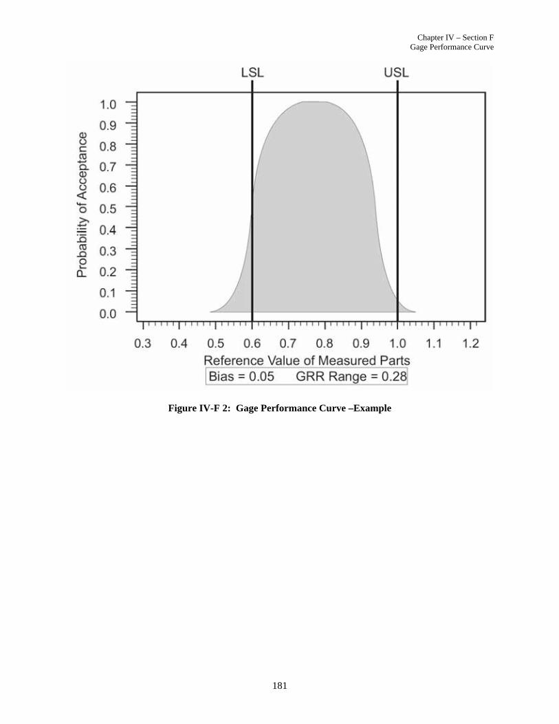
Chapter IV – Section F Gage Performance Curve
181
Figure IV-F 2: Gage Performance Curve –Example
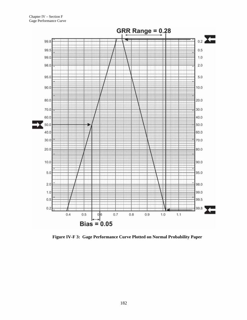
Chapter IV – Section F Gage Performance Curve
182
Figure IV-F 3: Gage Performance Curve Plotted on Normal Probability Paper
Chapter IV – Section G Reducing Variation Through Multiple Readings
183
Section G Reducing Variation Through Multiple Readings
If the variation of the present measurement system is not acceptable (over 30%), there is a method that can be used to reduce the variation to an acceptable level until proper measurement system improvements can be made. The unacceptable variation may be reduced by taking multiple statistically independent (non-correlated) measurement readings of the part characteristic being evaluated, determining the average of these measurements and letting the numeric value of the result be substituted for the individual measurement. This method will, of course, be time consuming, but is an alternative (with customer approval), until improvements are made to the measurement system (i.e., redesigning or buying a new system). The procedure for this alternative method is as follows:
1) Determine the number of multiple readings required to meet an
acceptable level of variation.
2) Follow the gage study procedure discussed earlier in this guideline.
Example: In the XYZ Corporate example, the percentage of tolerance GRR variation is 25.5%, with a 6 sigma spread equal to 0.24. The customer wants to reduce this figure to at least 15%, which would have an equivalent 6 sigma spread of 0.14. P
78F
To determine the number of multiple readings required to meet the desired 15% criteria, it must first be understood that the distribution of individual and average measurements has the same mean numeric value. Secondly, the variance of the distribution of averages is equal to the variance of the distribution of individuals divided by the sample size. Understanding this relationship as shown below, the number of multiple readings required can then be determined.
22 (6 )
(6 ) x n
This can be approximated by
(6 )(6 ) x
ss
n
and
0.240.14
n
78 See note on page vi.
Chapter IV – Section G Reducing Variation Through Multiple Readings
184
so
1.714n
and
n = 3 (rounded to nearest integer)
Therefore, 3 multiple readings on the part characteristic will reduce the total measurement system variation to approximately 0.14 and the %GRR to 15%.
This method should be considered as a temporary step until other improvements are made on the measurement system. This should be used only with the concurrence of the customer.

Chapter IV – Section H Pooled Standard Deviation Approach to GRR
185
Section H Pooled Standard Deviation Approach to GRR P
79
Analysis of a measurement system usually assumes that replicated data from all the part/specimens can be obtained from all the appraisers in a random fashion. This may not always be possible. If the measurement system analysis includes multiple locations it can be logistically unfeasible to demand a random sampling. Also some tests, notably chemical and metallurgical analyses (inter- and intra- laboratory studies), may require a cross section of diverse samples which are not part of a homogeneous process and may not be available at the same time.
These situations may be handled by using a nested DOE. An alternate approach is the pooled standard deviation GRR study which follows the methodology discussed in ASTM E691.
This approach views each part as a separate material and then computes the repeatability and reproducibility standard deviations as in E691. This will yield multiple separate values of repeatability and reproducibility. Since the parts are considered to be essentially identical, these separate estimates are assumed to be effectively identical. Of course they will never be exactly the same, but their average will give a good estimate of the true level of repeatability and similar reproducibility.
If this approach is used to evaluate a group of laboratories there is a concern of just what the nature of the “reproducibility” is. If this is greater than zero most of the time (that is for most of the materials) it should be interpreted as implying that there are differences between operators; i.e., in an interlaboratory program this would suggest that there are real differences between labs.
Although the E691 approach is typically used with a complete sample, it lends itself to a sequential approach. This is useful when all the samples are not available at the same time. It also can be used as part of the calibration process to maintain information on the measurement system’s variability.
The following study description assumes that the study will be applied in a sequential manner.
Conducting the Study Care should be taken to follow the “Preparation for Measurement System Study” shown in Chapter II, Section C.
Continue from step 6 on page 74:
79 Portions of this section including all of “Consistency Statistics” contributed by Neil Ullman of the American
Society for Testing and Materials (ASTM International).
Sequential Application
Chapter IV – Section H Pooled Standard Deviation Approach to GRR
186
7) Have each of the 2m appraisers evaluate the part for 3r readings. Record the data on the appropriate rows of a data collection sheet (see Sample Forms). (Note: Do not allow the appraisers to see their original reading while making these multiple checks.)
8) Calculate the average ( X ) and standard deviation (s) for the new part for each appraiser.
9) Plot the standard deviation values on the standard deviation chart and calculate the average standard deviation ( s ) (include all sub-group standard deviation for all appraisers). Draw this average standard deviation on the chart. Use the B4 factor for r samples to calculate the upper control limit for the standard deviation chart. Draw in this limit and determine if all values are in control (see Figure IV-H 1).
10) Plot the average ( X ) for each subgroup for all appraisers on the average chart (see Figure IV-H 1). The average values represent both process variation and measurement variation.
11) Calculate the grand average ( X ) (include all subgroup averages
( X ) for all appraisers). Draw this grand average ( X ) line on the chart.
12) Calculate the control limits for this chart using the A2 factor for r and average standard deviation ( s ) from the standard deviation chart; draw these limits on the average chart.
13) Analyze the data using the control charts and other graphical techniques as discussed in the Average and Range Method (see Chapter III).
14) Evaluate the measurement system’s parameters for each part by pooling the appraisers’ results.
2
1i
g
m
xi
x
s
sm
2
1i
g
m
si
g E
s
Repeatability sm
2
2 g
g g
E
g A x
sReproducibility s s
m
2 2
g g gg GRR E AGRR s s s
Chapter IV – Section H Pooled Standard Deviation Approach to GRR
187
E691 follows the convention wherein the MSA’s reproducibility is referred to as the appraiser variation and the MSA’s GRR is called reproducibility. In this case,
sappr = 2
2
3r
x
ss
sR = 2 2r apprs s
where sr = sE = Repeatability and sR = GRR = ASTM Reproducibility
15) Evaluate the overall measurement system’s parameters by pooling
the part results where g = number of parts.
2
1i
g
Ei
E
s
Repeatability sg
2
1i
g
Ai
A
s
Reproducibility sg
2
1i
g
GRRi
GRR
s
GRR sg
When calculating the percent of total variation, the historic standard deviation for the process should be used.
If the parts cover a wide variety of processes, for example different metallurgical or chemical specimens, the evaluation of percent total variation should be based on the process variation of specific specimens and not the total variation over all specimens.
Care should be given in the interpretation of the measurement system’s parameters in the case where appraisers are located in different facilities (e.g., laboratories).
The Repeatability will include between-equipment variation as well as within-equipment variation. This can be evaluated by calculating and comparing the repeatability within each location.
The Reproducibility will include between-location variation as well as between-appraiser variation. These components cannot be separated with this study.
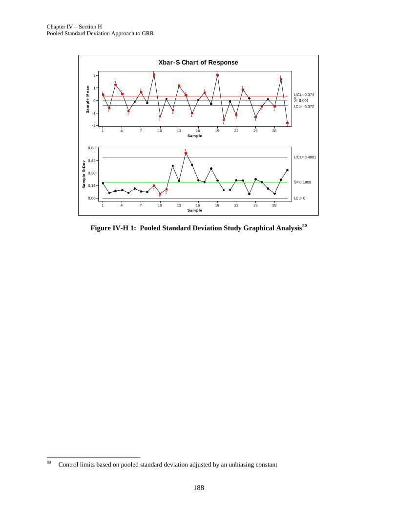
Chapter IV – Section H Pooled Standard Deviation Approach to GRR
188
28252219161310741
2
1
0
-1
-2
Sample
Sa
mp
le M
ea
n
__X=0.001
UC L=0.374
LC L=-0.372
28252219161310741
0.60
0.45
0.30
0.15
0.00
Sample
Sa
mp
le S
tDe
v
_S=0.1908
UC L=0.4901
LC L=0
1
1
11
1
1
1
1
1
1
1
1
1
1
1
1
1
1
1
1
1
1
1
22
2
Xbar-S Chart of Response
Figure IV-H 1: Pooled Standard Deviation Study Graphical Analysis P
80
80 Control limits based on pooled standard deviation adjusted by an unbiasing constant

Chapter IV – Section H Pooled Standard Deviation Approach to GRR
189
Table IV-H 1: Pooled Standard Deviation Analysis Data Set
Part
Acr
oss
Part
sT
rial
12
34
56
78
910
A1
0.29
-0.5
61.
340.
47-0
.80.
020.
59-0
.31
2.26
-1.3
62
0.41
-0.6
81.
170.
5-0
.92
-0.1
10.
75-0
.21.
99-1
.25
30.
64-0
.58
1.27
0.64
-0.8
4-0
.21
0.66
-0.1
72.
01-1
.31
xbar
0.44
67-0
.606
71.
2600
0.53
67-0
.853
3-0
.100
00.
6667
-0.2
267
2.08
67-1
.306
7xd
bbar
0.19
0333
33sd
0.17
790.
0643
0.08
540.
0907
0.06
110.
1153
0.08
020.
0737
0.15
040.
0551
appr
sd
0.10
2891
53
B1
0.08
-0.4
71.
190.
01-0
.56
-0.2
0.47
-0.6
31.
8-1
.68
20.
25-1
.22
0.94
1.03
-1.2
0.22
0.55
0.08
2.12
-1.6
23
0.07
-0.6
81.
340.
2-1
.28
0.06
0.83
-0.3
42.
19-1
.5xb
ar0.
1333
-0.7
900
1.15
670.
4133
-1.0
133
0.02
670 .
6167
-0.2
967
2.03
67-1
.600
0xd
bbar
0.06
8333
33sd
0.10
120.
3869
0.20
210.
5424
0.39
460.
2120
0.18
900.
3570
0.20
790.
0917
appr
sd
0.30
1739
4
C1
0.04
-1.3
80.
880.
14-1
.46
-0.2
90.
02-0
.46
1.77
-1.4
92
-0.1
1-1
.13
1.09
0.2
-1.0
7-0
.67
0.01
-0.5
61.
45-1
.77
3-0
.15
-0.9
60.
670.
11-1
.45
-0.4
90.
21-0
.49
1.87
-2.1
6xb
ar-0
.073
3-1
.156
70.
8800
0.15
00-1
.326
7-0
.483
30.
0800
-0.5
033
1.69
67-1
.806
7xd
bbar
-0.2
5433
333
sd0.
1002
0.21
130.
2100
0.04
580.
2223
0.19
010.
1127
0.05
130.
2194
0.33
65ap
pr s
d0.
1905
6058
sd x
bar
0.26
182
0.28
005
0.19
648
0.19
751
0.24
077
0.26
555
0.32
524
0.14
385
0.21
221
0.25
125
Poo
led
sd's
Rep
eata
bilit
y0.
1315
30.
2572
10.
1753
40.
3186
30.
2638
80.
1773
60.
1352
40.
2125
20.
1949
40.
2038
5po
oled
0.20
4274
0.19
5107
0.23
223
0.23
8896
0.22
9787
0.21
8795
0.21
8021
0.21
5578
0.21
4434
66R
epro
duci
bilit
y0.
2505
60.
2374
30.
1683
90.
0719
10.
1864
40.
2450
10.
3157
30.
0750
80.
1799
10.
2219
8po
oled
0.24
4086
0.22
1744
0.19
5372
0 .19
3619
0.20
3089
0.22
2696
0.20
9998
0.20
6871
0.20
8430
64G
RR
0.28
299
0.35
004
0.24
310
0.32
664
0.32
310
0.30
247
0.34
347
0.22
540
0.26
527
0.30
138
pool
ed0.
3182
850.
2953
590.
3034
810 .
3075
050.
3066
710.
3121
940.
3027
080.
2987
80.
2990
4106
ByPartresults
MeasurementSystem
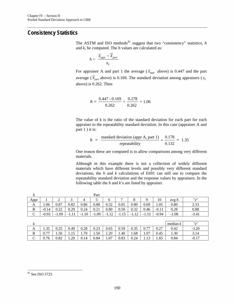
Chapter IV – Section H Pooled Standard Deviation Approach to GRR
190
Consistency Statistics
The ASTM and ISO methods P
81F suggest that two “consistency” statistics, h
and k, be computed. The h values are calculated as:
h = appr part
x
x x
s
For appraiser A and part 1 the average ( apprx above) is 0.447 and the part
average ( partx above) is 0.169. The standard deviation among appraisers ( xs
above) is 0.262. Then
0.447 - 0.169 0.278= = 1.06
0.262 0.262 = h
The value of k is the ratio of the standard deviation for each part for each appraiser to the repeatability standard deviation. In this case (appraiser A and part 1 ) it is:
standard deviation (appr A, part 1) 0.1781.35
repeatability 0.132 = = k
One reason these are computed is to allow comparisons among very different materials.
Although in this example there is not a collection of widely different materials which have different levels and possibly very different standard deviations, the h and k calculations of E691 can still use to compare the repeatability standard deviation and the response values by appraisers. In the following table the h and k’s are listed by appraiser.
h Part
Appr 1 2 3 4 5 6 7 8 9 10 avg h "z" A 1.06 0.87 0.82 0.86 0.88 0.32 0.65 0.80 0.69 1.05 0.80 2.53 B -0.14 0.22 0.29 0.24 0.21 0.80 0.50 0.32 0.46 -0.11 0.28 0.88 C -0.93 -1.09 -1.11 -1.10 -1.09 -1.12 -1.15 -1.12 -1.15 -0.94 -1.08 -3.41 k median k "z" A 1.35 0.25 0.49 0.28 0.23 0.65 0.59 0.35 0.77 0.27 0.42 -3.20 B 0.77 1.50 1.15 1.70 1.50 1.20 1.40 1.68 1.07 0.45 1.30 3.14 C 0.76 0.82 1.20 0.14 0.84 1.07 0.83 0.24 1.13 1.65 0.84 -0.17
81 See ISO 5725

Chapter IV – Section H Pooled Standard Deviation Approach to GRR
191
In the last two columns are the averages and a value of “z-value” to see if the appraisers are significantly different. The h values indicate that appraiser A is significantly high and appraiser C is significantly low in their readings of the size of the parts. It is also this significant difference which creates the GRR standard deviation.
The repeatability standard deviations can be also evaluate by looking at the k values. To do this, compute the median k and then an approximate “z score”. With this study, the expected median is about 0.861 with a standard deviation of approximately 0.439. The median k for appraiser A is then about –3.2 standard deviations below the expected level and appraiser B is as significantly high. So we see very great differences in the performance of just these three operators.
The graphs of h (Figure IV-H 2) and k (Figure IV-H 3) also help to illustrate these differences. Appraiser C has much lower results than the others. Similarly, the k values show how much lower appraiser A variation is with respect to repeatability. These are certainly issues to be examined about the performance of the measurement method as carried out by these appraisers.
h values
-1.5
-1
-0.5
0
0.5
1
1.5
0 1 2 3 4
Appraiser
A B C
Figure IV-H 2: Dot diagram of h values.
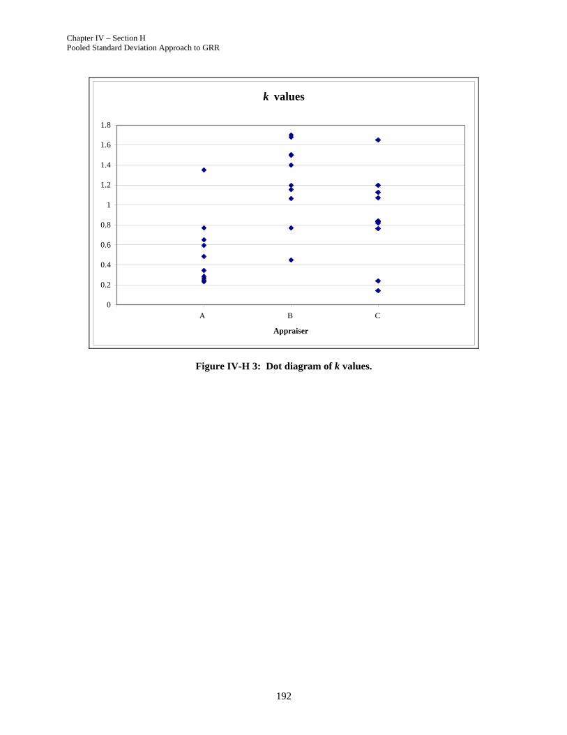
Chapter IV – Section H Pooled Standard Deviation Approach to GRR
192
k values
0
0.2
0.4
0.6
0.8
1
1.2
1.4
1.6
1.8
0 1 2 3 4
Appraiser
A B C
Figure IV-H 3: Dot diagram of k values.

Appendices
193
APPENDICES

194

Appendix A Analysis of Variance Concepts
195
Appendix A
Analysis of Variance Concepts
The GRR numerical analysis can be done following the formulas in Table A 3. This is what is called the Analysis of Variance (ANOVA) table. The ANOVA table is composed of six columns:
Source column is the cause of variation.
DF column is the degree of freedom associated with the source.
SS or sum of squares column is the deviation around the mean of the source.
MS or mean square column is the sum of squares divided by degrees of freedom.
EMS or expected mean square column determines the linear combination of variance components for each MS. The ANOVA table decomposes the total source of variation into four components: parts, appraisers, interaction of appraisers and parts, and replication error due to the gage/equipment repeatability.
The F-ratio column is calculated only for the interaction in a MSA ANOVA; it is determined by the mean square of interaction divided by mean square error.
The estimate of variance components for each source is given in Table A 1. F
82
Variance Estimate
Equipment (EV) 2eMS P
83
Interaction (INT) 2 AP eMS MS
r
Appraiser (AV) 2 A APMS MS
nr
Part (PV) 2 P APMS MS
kr
Table A 1: Estimate of Variance Components
Since each mean square is a sample quantity subject to sampling variation and the computations involve differences of mean squares, then negative variance component estimates are possible. This is a bit of a problem since the “master” variance components are equal or close to zero or have a small
82 In this table, all components of variation are assumed to be random effects. 83 In this application of ANOVA to measurement systems analysis, the ANOVA error term equates to the MSA
equipment variation, MSE.
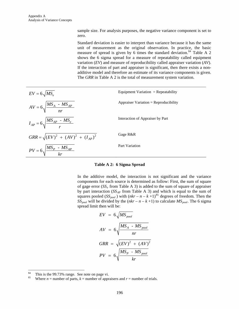
Appendix A Analysis of Variance Concepts
196
sample size. For analysis purposes, the negative variance component is set to zero.
Standard deviation is easier to interpret than variance because it has the same unit of measurement as the original observation. In practice, the basic measure of spread is given by 6 times the standard deviation. P
84F Table A 2
shows the 6 sigma spread for a measure of repeatability called equipment variation (EV) and measure of reproducibility called appraiser variation (AV). If the interaction of part and appraiser is significant, then there exists a non-additive model and therefore an estimate of its variance components is given. The GRR in Table A 2 is the total of measurement system variation.
6 eEV MS Equipment Variation = Repeatability
- 6 A APMS MS
AVnr
Appraiser Variation = Reproducibility
- 6 AP e
APMS MS
Ir
Interaction of Appraiser by Part
2 2 2( ) ( ) ( )APGRR EV AV I Gage R&R
- 6 P APMS MS
PVkr
Part Variation
Table A 2: 6 Sigma Spread
In the additive model, the interaction is not significant and the variance components for each source is determined as follow: First, the sum of square of gage error (SSe from Table A 3) is added to the sum of square of appraiser by part interaction (SSAP from Table A 3) and which is equal to the sum of squares pooled (SSpool ) with (nkr – n – k +1) P
85F degrees of freedom. Then the
SSpool will be divided by the (nkr – n – k +1) to calculate MSpool. The 6 sigma spread limit then will be:
6 poolEV MS
- 6 A poolMS MS
AVnr
2 2 ( ) ( )GRR EV AV
- 6 P poolMS MS
PVkr
84 This is the 99.73% range. See note on page vi. 85 Where n = number of parts, k = number of appraisers and r = number of trials.

Appendix A Analysis of Variance Concepts
197
In order to determine if the interaction is significant, compute the F statistic of appraiser by part interaction (see Table A 3). Compare this F statistic to an upper percentage point of an F distribution with numerator and denominator degrees of freedom taken from the ANOVA (Table A 3).
In order to decrease the risk of falsely concluding that there is no interaction effect, choose a high significance level. Once the GRR has been determined then the %GRR can be calculated in relation to process performance.
2 2.. ...
1
n
iP
i
x xSS
kr nkr
2 2. . ...
1
k
jA
j
x xSS
nr nkr
2
2 ...
1 1 1
n k r
ijmi j m
xTSS x
nkr
2 22 2. . ... ...
1 1 1 1
n k n k
ij jiAP
i j i j
x xx xSS
r kr nr nkr
[ ]e A P APSS TSS SS SS SS
Source DF SS MS F EMS
Appraiser k – 1 SSA MSA =
( 1)ASS
k
2 2 2r nr
Parts n – 1 SSP MSP =
( - 1)PSS
n
2 2 2r kr
Appraiser-by-Part (n – 1) (k – 1) SSAP MSAP =
( - 1) ( - 1)APSS
n k
AP
e
MS
MS 2 2r
Equipment nk (r – 1) SSe MSe =
( - 1)eSS
nk r
2
Total nkr – 1 TSS Appraiser ~ N( 20, )
Parts ~ N( 20, )
Appraiser x Part ~ N( 20, )
Equipment ~ N( 20, )
Table A 3: Analysis of Variance (ANOVA)
Tables A 4 and A 5 show the ANOVA calculations for our example data from Figure III-B 15.

Appendix A Analysis of Variance Concepts
198
Source DF SS MS F EMS
Appraiser 2 3.1673 1.58363 79.41* 2 2 23 30
Parts 9 88.3619 9.81799 492.29* 2 2 23 9
Appraiser by Part 18 0.3590 0.01994 0.434 2 23
Equipment 60 2.7589 0.04598 2
Total 89 94.6471
* Significant at = 0.05 level
Table A 4: Tabulated ANOVA Results
Since the calculated F value for the interaction (0.434) is less than the critical value of , ,F 18 60 , the interaction term
is pooled with the equipment (error) term. That is, the estimate of variance is based on the model without interaction.
Estimate of Variance
Std. Dev. ()
6 () % Total Variation % Contribution
2 = 0.039973 (Equipment)
0.199933 EV = 1.199598 18.4 3.4
2 = 0.051455 (Appraiser)
0.226838 AV = 1.361028 20.9 4.4
2 = 0
(Interaction)
INT = 0 0 0
GRR = 0.09143
( 2 2 2 )
0.302373 GRR = 1.814238 27.9 7.8
2 = 1.086447
(Part)
1.042327 PV = 6.253962 96.0 92.2
Total Variation 1.085 TV = 6.51 100.0
Table A 5: Tabulated ANOVA Results
1.41( / ) 1.41(6.25/1.81) 4.87 4 ndc PV GRR
2 2 ( ) Total Variation TV GRR PV
( ) ( )
( ) ( )
6% 100 100
6
components components
total total
of Total Variation
2 2( ) ( )
2 2( ) ( )
6% ( ) 100 100
6
components components
total total
Contribution Total Variance

Appendix B Impact of GRR on the Capability Index Cp
199
Appendix B
Impact of GRR on the Capability Index Cp
Formulas:
2 2 2Obs Act Meas (1)
where Obs = the observed process variation Act = the actual process variation Meas = the measurement system variation
6xx
U LCp
(2)
where U, L are the upper and lower specification values x = Obs or Act as defined in (1)
% *100%pGRR GRR (3)
based on process variation:
6Meas
pObs
kGRR
(4)
Note: 1pGRR since 2 2Obs Meas by equation (1)
based on the tolerance range:
Measp
kGRR
U L
(5)
In (4) and (5), k is normally taken to be 6.
Analysis:
* ActObs Act
Obs
Cp Cp
2 2
* Obs MeasAct
Obs
Cp
using (1)
with GRR based on the process variation 21
* ObsObs Act
Obs
GRRCp Cp
using (4)
2* 1ActCp GRR (6)
or

Appendix B Impact of GRR on the Capability Index Cp
200
21Obs
Act
CpCp
GRR
(6’)
with GRR based on the tolerance range
1* Meas
Obs Obs
GRRCp
using (2) and (5)
consequently
2* 1 *Obs Act ObsCp Cp Cp GRR (7)
and
21 *
ObsAct
Obs
CpCp
Cp GRR
(7’)

Appendix B Impact of GRR on the Capability Index Cp
201
Graphical Analysis Based on (6), the family of lines for CpObs with respect to CpAct is:
Figure B 1: Observed vs. Actual Cp (process based)
Actual GRR
10% 20% 30% 40% 50% 60% 70% 90%
Observed Cp with Cp based on Process Range
1.3 1.29 1.27 1.24 1.19 1.13 1.04 0.93 0.57
Observed Cp with Cp based on the Tolerance
1.3 1.29 1.26 1.20 1.11 0.99 0.81 0.54 never
Table B 1: Comparison of Observed to Actual Cp
Ob
ser
ved
Cp
0
0.5
1
1.5
2
2.5
3
3.5
0.5 1 1.5 2 2.5 3
Actual Cp
10 %30 %50%
70%
90%
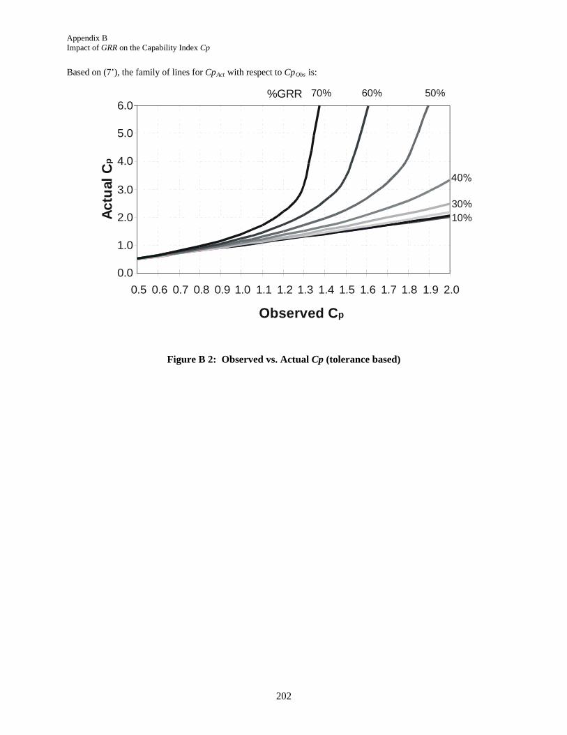
Appendix B Impact of GRR on the Capability Index Cp
202
Based on (7’), the family of lines for CpAct with respect to CpObs is:
Figure B 2: Observed vs. Actual Cp (tolerance based)
0.0
1.0
2.0
3.0
4.0
5.0
6.0
0.5 0.6 0.7 0.8 0.9 1.0 1.1 1.2 1.3 1.4 1.5 1.6 1.7 1.8 1.9 2.0
Observed Cp
Act
ual
Cp
%GRR 70% 60% 50%
30%10%
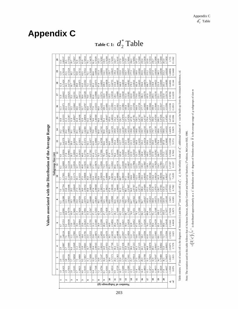
Appendix C *2d Table
203
Appendix C Table C 1:
*2d Table
Val
ues
ass
ocia
ted
wit
h th
e D
istr
ibu
tion
of
the
Ave
rage
Ran
ge
Sub
grou
p S
ize
()
m
2 3
4 5
6 7
8 9
10
11
12
13
14
15
16
17
18
19
20
1 1.
0 1.
4142
1 2.
0 1.
9115
5
2.9
2.23
887
3.8
2.48
124
4.7
2.67
253
5.5
2.82
981
6.3
2.96
288
7.0
3.07
794
7.7
3.17
905
8.3
3.26
909
9.0
3.35
016
9.6
3.42
378
10.2
3.
4911
6
10.8
3.
5533
3 11
.3
3.61
071
11.9
3.
6642
2 12
.4
3.71
424
12.9
3.
7611
8
13.4
3.
8053
7 2
1.9
1.27
931
3.8
1.80
538
5.7
2.15
069
7.5
2.40
484
9.2
2.60
438
10.8
2.
7677
9 12
.3
2.90
562
13.8
3.
0244
6 15
.1
3.12
869
16.5
3.
2213
4 17
.8
3.30
463
19.0
3.
3801
7 20
.2
3.44
922
21.3
3.
5128
7 22
.4
3.57
156
23.5
3.
6262
5 24
.5
3.67
734
25.5
3.
7252
4 26
.5
3.77
032
3 2.
8 1.
2310
5 5.
7 1.
7685
8 8.
4 2.
1204
9 11
.1
2.37
883
13.6
2.
5812
7 16
.0
2.74
681
18.3
2.
8862
8 20
.5
3.00
643
22.6
3.
1117
3
24.6
3.
2052
6 26
.5
3.28
931
28.4
3.
3655
0 30
.1
3.43
512
31.9
3.
4992
7 33
.5
3.55
842
35.1
3.
6135
1 36
.7
3.66
495
38.2
3.
7131
9 39
.7
3.75
857
4 3.
7 1.
2062
1 7.
5 1.
7498
9 11
.2
2.10
522
14.7
2.
3657
1 18
.1
2.56
964
21.3
2.
7362
6 24
.4
2.87
656
27.3
2.
9973
7 30
.1
3.10
321
32.7
3.
1972
0 35
.3
3.28
163
37.7
3.
3581
5 40
.1
3.42
805
42.4
3.
4924
6 44
.6
3.55
183
46.7
3.
6071
2 48
.8
3.65
875
50.8
3.
7071
5 52
.8
3.75
268
5 4.
6 1.
1910
5 9.
3 1.
7385
7 13
.9
2.09
601
18.4
2.
3578
1 22
.6
2.56
263
26.6
2.
7299
1 30
.4
2.87
071
34.0
2.
9919
2 37
.5
3.09
808
40.8
3.
1923
5 44
.0
3.27
701
47.1
3.
3537
2 50
.1
3.42
381
52.9
3.
4883
6 55
.7
3.54
787
58.4
3.
6032
8 61
.0
3.65
502
63.5
3.
7035
2 65
.9
3.74
914
6 5.
5 1.
1808
3 11
.1
1.73
099
16.7
2.
0898
5 22
.0
2.35
253
27.0
2.
5579
5 31
.8
2.72
567
36.4
2.
8668
0 40
.8
2.98
829
45.0
3.
0946
7 49
.0
3.18
911
52
.8
3.27
392
56.5
3.
3507
7 60
.1
3.42
097
63.5
3.
4856
3 66
.8
3.54
522
70.0
3.
6007
2 73
.1
3.65
253
76.1
3.
7010
9 79
.1
3.74
678
7 6.
4 1.
1734
8 12
.9
1.72
555
19.4
2.
0854
3 25
.6
2.34
875
31.5
2.
5546
0 37
.1
2.72
263
42.5
2.
8640
1 47
.6
2.98
568
52.4
3.
0922
2 57
.1
3.18
679
61.6
3.
2717
2 65
.9
3.34
866
70.0
3.
4189
4 74
.0
3.48
368
77.9
3.
5433
3 81
.6
3.59
888
85.3
3.
6507
5 88
.8
3.69
936
92.2
3.
7450
9 8
7.2
1.16
794
14.8
1.
7214
7 22
.1
2.08
212
29.2
2.
3459
1 36
.0
2.55
208
42.4
2.
7203
6 48
.5
2.86
192
54.3
2.
9837
3 59
.9
3.09
039
65.2
3.
1850
6 70
.3
3.27
006
75.2
3.
3470
8 80
.0
3.41
742
84.6
3.
4822
1 89
.0
3.54
192
93.3
3.
5975
1 97
.4
3.64
941
101.
4 3.
6980
6 10
5.3
3.74
382
9 8.
1 1.
1636
1 16
.6
1.71
828
24.9
2.
0795
3 32
.9
2.34
370
40.4
2.
5501
3 47
.7
2.71
858
54.5
2.
8602
8 61
.1
2.98
221
67.3
3.
0889
6 73
.3
3.18
370
79.1
3.
2687
8 84
.6
3.34
585
90.0
3.
4162
4 95
.1
3.48
107
100.
1 3.
5408
1 10
4.9
3.59
644
109.
5 3.
6483
8 11
4.1
3.
6970
5 11
8.5
3.
7428
4 10
9.
0 1.
1601
4 18
.4
1.71
573
27.6
2.
0774
6 36
.5
2.34
192
44.9
2.
5485
6 52
.9
2.71
717
60.6
2.
8589
8 67
.8
2.98
100
74.8
3.
0878
1 81
.5
3.18
262
87.9
3.
2677
5 94
.0
3.34
486
99.9
3.
4152
9 10
5.6
3.48
016
111.
2
3.53
993
116.
5
3.59
559
121.
7 3.
6475
5 12
6.7
3.69
625
131.
6 3.
7420
5 11
9.
9 1.
1572
9 20
.2
1.71
363
30.4
2.
0757
7 40
.1
2.34
048
49.4
2.
5472
8 58
.2
2.71
600
66.6
2.
8579
1 74
.6
2.98
000
82.2
3.
0868
8 89
.6
3.18
174
96.6
3.
2669
0 10
3.4
3.34
406
109.
9 3.
4145
2 11
6.2
3.
4794
1 12
2.3
3.53
921
128.
1 3.
5948
9 13
3.8
3.64
687
139.
4 3.
6955
8 14
4.7
3.74
141
12
10.7
1.
1549
0 22
.0
1.71
189
33
.1
2.07
436
43.7
2.
3392
7 53
.8
2.54
621
63.5
2.
7150
4 72
.6
2.85
702
81.3
2.
9791
7 89
.7
3.08
610
97.7
3.
1810
0 10
5.4
3.26
620
112.
7
3.34
339
119.
9
3.41
387
126.
7 3.
4787
9 13
3.3
3.53
861
139.
8 3.
5943
0 14
6.0
3.64
630
152.
0 3.
6950
3 15
7.9
3.74
087
13
11.6
1.
1528
9 23
.8
1.71
041
35.8
2.
0731
6 47
.3
2.33
824
58.3
2.
5453
0 68
.7
2.71
422
78.6
2.
8562
7 88
.1
2.97
847
97.1
3.
0854
4 10
5.8
3.18
037
114.
1
3.26
561
122.
1 3.
3428
2 12
9.8
3.41
333
137.
3 3.
4782
6 14
4.4
3.53
810
151.
4 3.
5938
1 15
8.1
3.64
582
164.
7 3.
6945
7 17
1.0
3.74
041
14
12.5
1.
1511
5
25.7
1.
7091
4 38
.6
2.07
213
51.0
2.
3373
7 62
.8
2.54
452
74.0
2.
7135
1 84
.7
2.85
562
94.9
2.
9778
7 10
4.6
3.08
487
113.
9
3.17
984
122.
9 3.
2651
0 13
1.5
3.34
233
139.
8 3.
4128
6 14
7.8
3.47
781
155.
5 3.
5376
6 16
3.0
3.59
339
170.
3 3.
6454
1 17
7.3
3.69
417
184.
2 3.
7400
2 15
13
.4
1.14
965
27.5
1.
7080
4 41
.3
2.07
125
54.6
2.
3366
1 67
.2
2.54
385
79.3
2.
7129
0 90
.7
2.85
506
101.
6 2.
9773
5 11
2.1
3.
0843
8 12
2.1
3.17
938
131.
7 3.
2646
5 14
0.9
3.34
191
149.
8 3.
4124
5 15
8.3
3.47
742
166.
6 3.
5372
8 17
4.6
3.59
302
182.
4 3.
6450
5 19
0.0
3.69
382
197.
3 3.
7396
9 16
14
.3
1.14
833
29.3
1.
7070
8 44
.1
2.07
047
58.2
2.
3359
4 71
.7
2.54
326
84.5
2.
7123
7 96
.7
2.85
457
108.
4 2.
9768
9 11
9.5
3.
0839
5 13
0.2
3.17
897
140.
4 3.
2642
7 15
0.2
3.34
154
159.
7 3.
4121
0 16
8.9
3.47
707
177.
7 3.
5369
5 18
6.3
3.59
270
194.
6 3.
6447
4 20
2.6
3.69
351
210.
4 3.
7393
9 17
15
.1
1.14
717
31.1
1.
7062
3 46
.8
2.06
978
61.8
2.
3353
5 76
.2
2.54
274
89.8
2.
7119
0
102.
8 2.
8541
3 11
5.1
2.
9764
9 12
7.0
3.08
358
138.
3 3.
1786
1 14
9.2
3.26
393
159.
6 3.
3412
1 16
9.7
3.41
178
17
9.4
3.47
677
188.
8 3.
5366
6 19
7.9
3.59
242
206.
7 3.
6444
7 21
5.2
3.69
325
223.
6 3.
7391
3 18
16
.0
1.14
613
32.9
1.
7054
7 49
.5
2.06
917
65.5
2.
3348
3 80
.6
2.54
228
95.1
2.
7114
8
108.
8 2.
8537
5 12
1.9
2.97
613
134.
4 3.
0832
4 14
6.4
3.17
829
157.
9 3.
2636
2 16
9.0
3.34
092
179.
7 3.
4115
0
190.
0 3.
4765
0 19
9.9
3.53
640
209.
5 3.
5921
6 21
8.8
3.64
422
227.
9 3.
6930
1 23
6.7
3.73
890
19
16.9
1.
1452
0 34
.7
1.70
480
52.3
2.
0686
2 69
.1
2.33
436
85.1
2.
5418
7 10
0.3
2.71
111
11
4.8
2.
8534
1 12
8.7
2.97
581
141.
9 3.
0829
4 15
4.5
3.17
801
166.
7 3.
2633
5 17
8.4
3.34
066
189.
6 3.
4112
5
200.
5 3.
4762
6 21
1.0
3.
5361
7 22
1.1
3.59
194
231.
0 3.
6440
0 24
0.5
3.69
280
249.
8 3.
7386
9
NumberofSubgroups(g)
20
17.8
1.
1443
7 36
.5
1.70
419
55.0
2.
0681
3 72
.7
2.33
394
89.6
2.
5414
9 10
5.6
2.71
077
120.
9 2.
8531
0 13
5.4
2.97
552
149.
3 3.
0826
7 16
2.7
3.17
775
175.
5 3.
2631
1
187.
8 3.
3404
2 19
9.6
3.41
103
21
1.0
3.
4760
5 22
2.1
3.53
596
232.
8 3.
5917
4 24
3.1
3.64
380
253.
2 3.
6926
0 26
3.0
3.73
850
d 2
1.12
838
1.69
257
2.05
875
2.32
593
2.53
441
2.70
436
2.84
72
2.97
003
3.07
751
3.17
287
3.25
846
3.33
598
3.40
676
3.47
193
3.53
198
3.58
788
3.64
006
3.68
896
3.73
5 cd
0.
876
1.81
5 2.
7378
3.
623
4.46
58
5.26
73
6.03
05
6.75
82
7.45
39
8.12
07
8.76
02
9.37
51
9.96
79
10.5
396
11.0
913
11
.625
9 12
.144
12
.646
8 13
.136
2
Tabl
e en
trie
s: 1
st li
ne o
f ea
ch c
ell i
s th
e de
gree
s of
fre
edom
()
and
the
2nd li
ne o
f ea
ch c
ell i
s
; is
the
infi
nity
val
ue o
f : a
ddit
iona
l val
ues
of
can
be b
uilt
up f
rom
the
cons
tant
dif
fere
nce,
.
cd
Not
e: T
he n
otat
ion
used
in th
is ta
ble
follo
ws
that
of A
ches
on D
unca
n, Q
ualit
y C
ontr
ol a
nd I
ndus
tria
l Sta
tistic
s,5th
edit
ion,
McG
raw
-Hil
l, 19
86.
2
2R
is d
istr
ibut
ed a
ppro
xim
atel
y as
a
2 d
istr
ibut
ion
with
d
egre
es o
f fr
eedo
m w
here
R is
the
aver
age
rang
e of
g s
ubgr
oups
of
size
m
2d2d*
2d*
2d*

204
Appendix D Gage R Study
205
Appendix D
Gage R Study Application:
Offers a preliminary determination of short-term gage repeatability only.
May be used for screening before shipment from gage supplier.
May be used in pre-production when part availability is minimal.
May be used during gage development – e.g., for quickly comparing different clamping locations; comparing different methodologies.
This method CANNOT be used for final gage acceptance without other more complete and detailed MSA methods.
Assumptions:
Process stability and variation cannot be known at this point in time.
Linearity and bias are not issues.
Reproducibility is not considered here. The purpose is to focus on gage repeatability alone.
I/MR (Individual/Moving Range) chart will provide minimal assessment of stability.
Analyze by:
Take one part, one operator; place part in fixture, measure; take part out of fixture; repeat this 9 more times with the same part and same operator.
Plot data on I/MR chart; assess stability. If data appears unstable, perform corrective action. P
86
If stable, calculate sigma of individuals by using either s for all readings or *2/MR d ; multiply by 6; divide this value by the characteristic tolerance;
multiply by 100%. Review %Repeatability against previously established gage acceptability standards, or use for comparative purposes during gage development.
86 Some judgment may be needed here, as 10 subgroups of individual data is insufficient to establish stability;
however, obvious instabilities may still be assessed and provide value to the analysis.

Appendix D Gage R Study
206
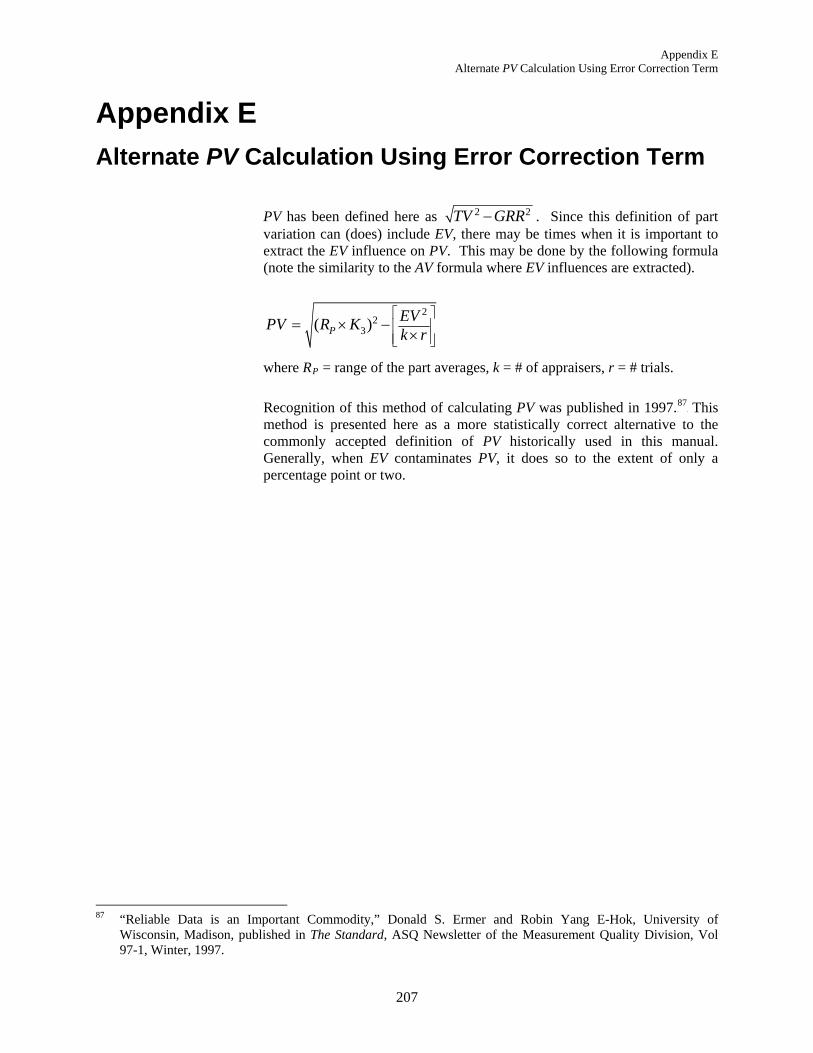
Appendix E Alternate PV Calculation Using Error Correction Term
207
Appendix E
Alternate PV Calculation Using Error Correction Term
PV has been defined here as 2 2TV GRR . Since this definition of part variation can (does) include EV, there may be times when it is important to extract the EV influence on PV. This may be done by the following formula (note the similarity to the AV formula where EV influences are extracted).
22
3( )PEVPV R Kk r
where RP = range of the part averages, k = # of appraisers, r = # trials.
Recognition of this method of calculating PV was published in 1997. P
87F This
method is presented here as a more statistically correct alternative to the commonly accepted definition of PV historically used in this manual. Generally, when EV contaminates PV, it does so to the extent of only a percentage point or two.
87 “Reliable Data is an Important Commodity,” Donald S. Ermer and Robin Yang E-Hok, University of
Wisconsin, Madison, published in The Standard, ASQ Newsletter of the Measurement Quality Division, Vol 97-1, Winter, 1997.

Appendix E Alternate PV Calculation Using Error Correction Term
208
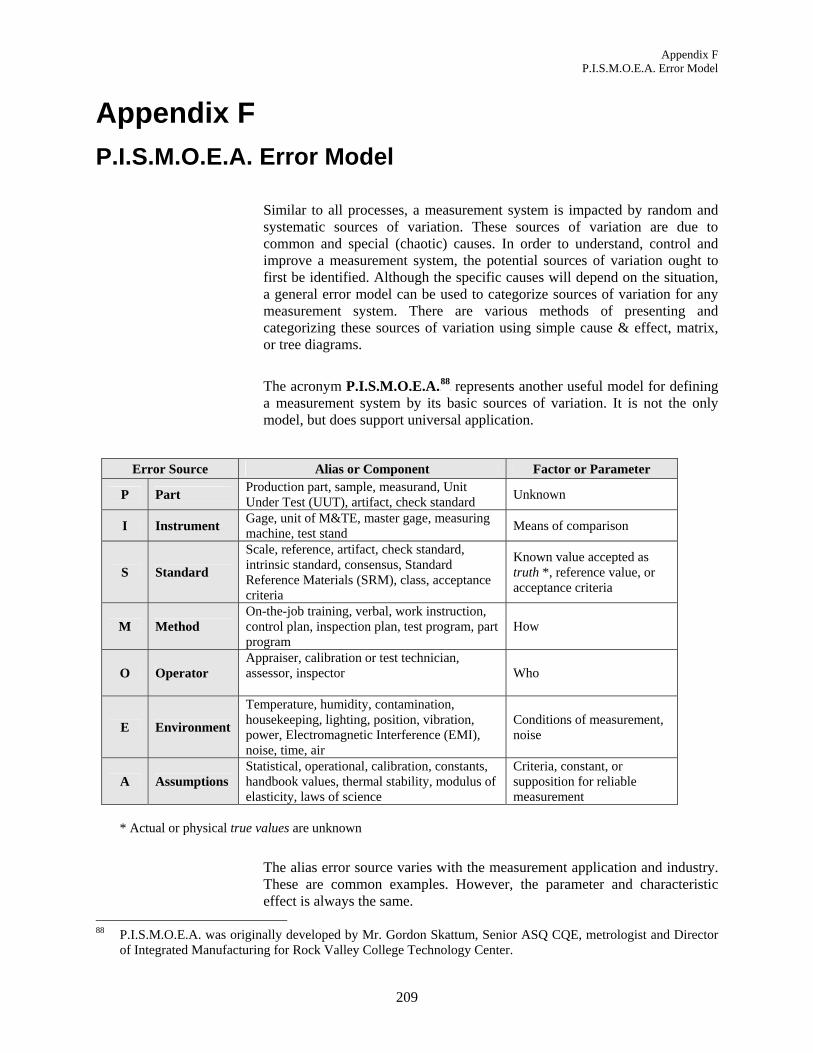
Appendix F P.I.S.M.O.E.A. Error Model
209
Appendix F
P.I.S.M.O.E.A. Error Model
Similar to all processes, a measurement system is impacted by random and systematic sources of variation. These sources of variation are due to common and special (chaotic) causes. In order to understand, control and improve a measurement system, the potential sources of variation ought to first be identified. Although the specific causes will depend on the situation, a general error model can be used to categorize sources of variation for any measurement system. There are various methods of presenting and categorizing these sources of variation using simple cause & effect, matrix, or tree diagrams.
The acronym P.I.S.M.O.E.A. P
88F represents another useful model for defining
a measurement system by its basic sources of variation. It is not the only model, but does support universal application.
Error Source Alias or Component Factor or Parameter
P Part Production part, sample, measurand, Unit Under Test (UUT), artifact, check standard
Unknown
I Instrument Gage, unit of M&TE, master gage, measuring machine, test stand
Means of comparison
S Standard
Scale, reference, artifact, check standard, intrinsic standard, consensus, Standard Reference Materials (SRM), class, acceptance criteria
Known value accepted as truth *, reference value, or acceptance criteria
M Method On-the-job training, verbal, work instruction, control plan, inspection plan, test program, part program
How
O Operator Appraiser, calibration or test technician, assessor, inspector
Who
E Environment
Temperature, humidity, contamination, housekeeping, lighting, position, vibration, power, Electromagnetic Interference (EMI), noise, time, air
Conditions of measurement, noise
A Assumptions Statistical, operational, calibration, constants, handbook values, thermal stability, modulus of elasticity, laws of science
Criteria, constant, or supposition for reliable measurement
* Actual or physical true values are unknown
The alias error source varies with the measurement application and industry. These are common examples. However, the parameter and characteristic effect is always the same.
88 P.I.S.M.O.E.A. was originally developed by Mr. Gordon Skattum, Senior ASQ CQE, metrologist and Director
of Integrated Manufacturing for Rock Valley College Technology Center.
Appendix F P.I.S.M.O.E.A. Error Model
210
All methods of Measurement Systems Analysis are quality tools. All quality tools are based on assumptions. If you violate the assumptions, the tool becomes unpredictable at best and could lead to a false conclusion at worst.
The typical statistical assumptions of a Gage R&R study, include: normal process, random and independent trials, stable, and test-retest criteria. When one or more assumption is violated (e.g., non-normal measurement process, operator bias) the tool and analysis ultimately become unstable, confusing, and misleading. %GRR evaluations for product and process control can be overestimated. There are also non-statistical assumptions related to measurement systems (e.g., calibration, operational, coefficients and rates of expansion, physical laws and constants). The measurement planner should be able to identify, control, correct, or modify the MSA method to accommodate significant violations for the assumptions in the measurement process.
Violation of the test-retest criteria is always a consideration for destructive test or in-process measurement systems where the feature is changing. The measurement planner ought to consider appropriate hybrids, modifications, or alternative techniques to the standard measurement system study.
Assumptions tend to contribute greater to total measurement variation when: 1) using more powerful methods or tools (e.g., ANOVA, regression analysis, designed experiments, probability predictions, and control charts), and 2) as measurement precision increases. High precision measurement applications must often plan for, and sometimes apply, correction for coefficients and thermal expansion, deformation, creep or other assumptions in the measurement process.
The greatest danger for a quality analyst or measurement planner regarding assumptions is that it is assumed they are insignificant or constant and therefore too often ignored.
Table F 1 demonstrates examples of the PISMOEA model for three different measurement situations.
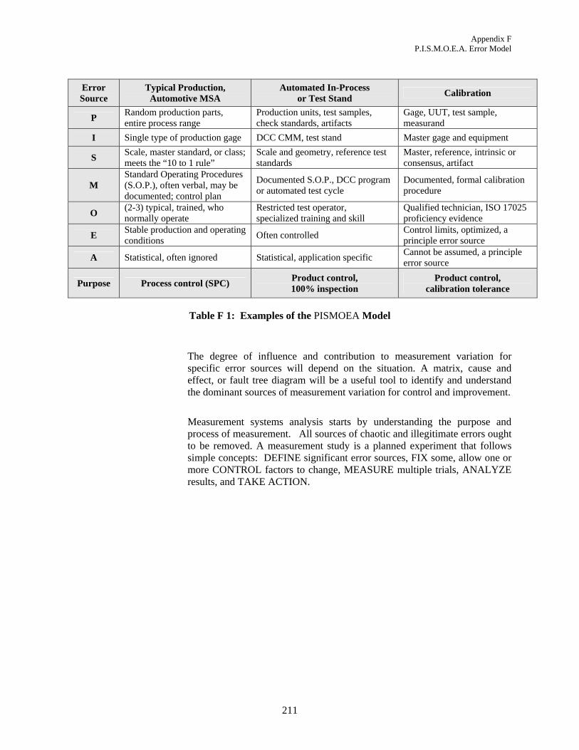
Appendix F P.I.S.M.O.E.A. Error Model
211
Error Source
Typical Production, Automotive MSA
Automated In-Process or Test Stand
Calibration
P Random production parts, entire process range
Production units, test samples, check standards, artifacts
Gage, UUT, test sample, measurand
I Single type of production gage DCC CMM, test stand Master gage and equipment
S Scale, master standard, or class; meets the “10 to 1 rule”
Scale and geometry, reference test standards
Master, reference, intrinsic or consensus, artifact
M Standard Operating Procedures (S.O.P.), often verbal, may be documented; control plan
Documented S.O.P., DCC program or automated test cycle
Documented, formal calibration procedure
O (2-3) typical, trained, who normally operate
Restricted test operator, specialized training and skill
Qualified technician, ISO 17025 proficiency evidence
E Stable production and operating conditions
Often controlled Control limits, optimized, a principle error source
A Statistical, often ignored Statistical, application specific Cannot be assumed, a principle error source
Purpose Process control (SPC) Product control, 100% inspection
Product control, calibration tolerance
Table F 1: Examples of the PISMOEA Model
The degree of influence and contribution to measurement variation for specific error sources will depend on the situation. A matrix, cause and effect, or fault tree diagram will be a useful tool to identify and understand the dominant sources of measurement variation for control and improvement.
Measurement systems analysis starts by understanding the purpose and process of measurement. All sources of chaotic and illegitimate errors ought to be removed. A measurement study is a planned experiment that follows simple concepts: DEFINE significant error sources, FIX some, allow one or more CONTROL factors to change, MEASURE multiple trials, ANALYZE results, and TAKE ACTION.

Glossary
212

Glossary
213
Glossary See the Statistical Process Control (SPC) Reference Manual for additional glossary definitions. 5.15 vs. 6 GRRσ Multiplying Factor See note on page iv.
Accuracy The closeness of agreement between an observed value and the
accepted reference value. Analysis of Variance A statistical method (ANOVA) often used in designed experiments
(DOE), to analyze variable data from multiple groups in order to compare means and analyze sources of variation.
Apparent Resolution The size of the least increment on the measurement instrument is the
apparent resolution. This value is typically used in literature as advertisement to classify the measurement instrument. The number of data categories can be determined by dividing the size into the expected process distribution spread ( 6 ).
NOTE: The number of digits displayed or reported does not always indicate the resolution of the instrument. For example, parts measured as 29.075, 29.080, 29.095, etc., are recorded as five (5) digit measurements. However, the instrument may not have a resolution of .001 but rather .005.
Appraiser Variation The variation in average measurements of the same part (measurand)
between different appraisers (operators) using the same measuring instrument and method in a stable environment. Appraiser variation (AV) is one of the common sources of measurement system variation (error) that results from differences in operator skill or technique using the same measurement system. Appraiser variation is commonly assumed to be the “reproducibility error” associated with a measurement system; this is not always true (see Reproducibility).
Bayes’ Theorem A mathematical formula used for calculating conditional probabilities.
The probability of a hypothesis G conditional on a given body of data M is the ratio of the unconditional probability of the conjunction of the hypothesis with the data to the unconditional probability of the data alone The probability of G conditional on M is defined as PRM T(G) = P(G & M)/P(G), provided that both terms of this ratio exist and P(G) > 0
Bias The difference between the observed average of measurements (trials
under repeatability conditions) and a reference value; historically referred to as accuracy. Bias is evaluated and expressed at a single point within the operating range of the measurement system.
Calibration A set of operations that establish, under specified conditions, the relationship between a measuring device and a traceable standard of known reference value and uncertainty. Calibration may also include steps to detect, correlate, report, or eliminate by adjustment any discrepancy in accuracy of the measuring device being compared.
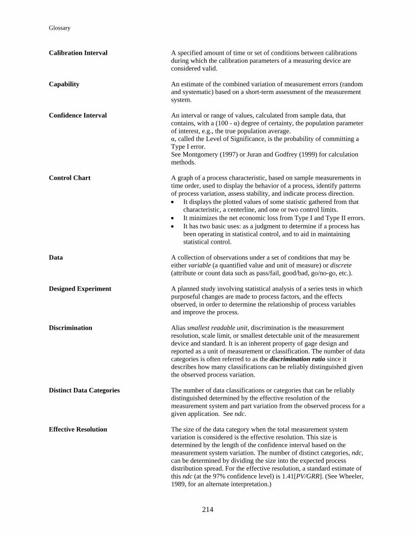
Glossary
214
Calibration Interval A specified amount of time or set of conditions between calibrations during which the calibration parameters of a measuring device are considered valid.
Capability An estimate of the combined variation of measurement errors (random
and systematic) based on a short-term assessment of the measurement system.
Confidence Interval An interval or range of values, calculated from sample data, that
contains, with a (100 - α) degree of certainty, the population parameter of interest, e.g., the true population average. α, called the Level of Significance, is the probability of committing a Type I error. See Montgomery (1997) or Juran and Godfrey (1999) for calculation methods.
Control Chart A graph of a process characteristic, based on sample measurements in
time order, used to display the behavior of a process, identify patterns of process variation, assess stability, and indicate process direction. It displays the plotted values of some statistic gathered from that
characteristic, a centerline, and one or two control limits. It minimizes the net economic loss from Type I and Type II errors. It has two basic uses: as a judgment to determine if a process has
been operating in statistical control, and to aid in maintaining statistical control.
Data A collection of observations under a set of conditions that may be
either variable (a quantified value and unit of measure) or discrete (attribute or count data such as pass/fail, good/bad, go/no-go, etc.).
Designed Experiment A planned study involving statistical analysis of a series tests in which
purposeful changes are made to process factors, and the effects observed, in order to determine the relationship of process variables and improve the process.
Discrimination Alias smallest readable unit, discrimination is the measurement
resolution, scale limit, or smallest detectable unit of the measurement device and standard. It is an inherent property of gage design and reported as a unit of measurement or classification. The number of data categories is often referred to as the discrimination ratio since it describes how many classifications can be reliably distinguished given the observed process variation.
Distinct Data Categories The number of data classifications or categories that can be reliably
distinguished determined by the effective resolution of the measurement system and part variation from the observed process for a given application. See ndc.
Effective Resolution The size of the data category when the total measurement system
variation is considered is the effective resolution. This size is determined by the length of the confidence interval based on the measurement system variation. The number of distinct categories, ndc, can be determined by dividing the size into the expected process distribution spread. For the effective resolution, a standard estimate of this ndc (at the 97% confidence level) is 1.41[PV/GRR]. (See Wheeler, 1989, for an alternate interpretation.)
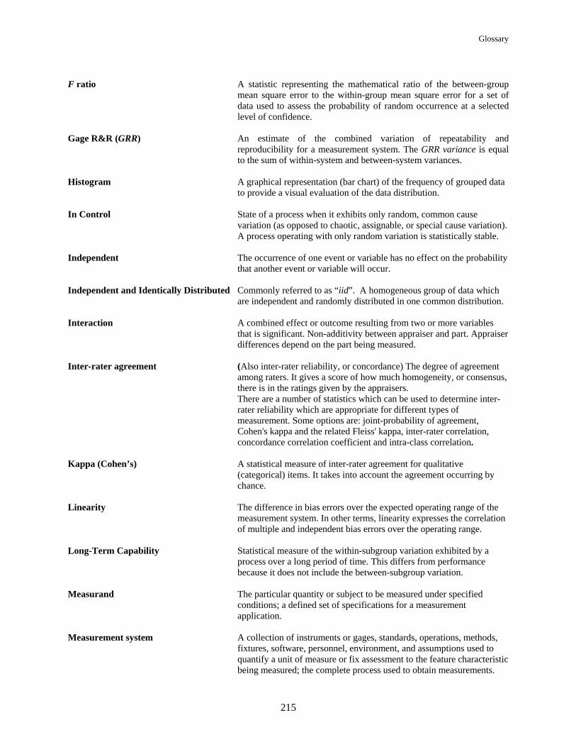
Glossary
215
F ratio A statistic representing the mathematical ratio of the between-group
mean square error to the within-group mean square error for a set of data used to assess the probability of random occurrence at a selected level of confidence.
Gage R&R (GRR) An estimate of the combined variation of repeatability and
reproducibility for a measurement system. The GRR variance is equal to the sum of within-system and between-system variances.
Histogram A graphical representation (bar chart) of the frequency of grouped data
to provide a visual evaluation of the data distribution. In Control State of a process when it exhibits only random, common cause
variation (as opposed to chaotic, assignable, or special cause variation). A process operating with only random variation is statistically stable.
Independent The occurrence of one event or variable has no effect on the probability
that another event or variable will occur. Independent and Identically Distributed Commonly referred to as “iid”. A homogeneous group of data which
are independent and randomly distributed in one common distribution. Interaction A combined effect or outcome resulting from two or more variables
that is significant. Non-additivity between appraiser and part. Appraiser differences depend on the part being measured.
Inter-rater agreement (Also inter-rater reliability, or concordance) The degree of agreement
among raters. It gives a score of how much homogeneity, or consensus, there is in the ratings given by the appraisers. There are a number of statistics which can be used to determine inter-rater reliability which are appropriate for different types of measurement. Some options are: joint-probability of agreement, Cohen's kappa and the related Fleiss' kappa, inter-rater correlation, concordance correlation coefficient and intra-class correlation.
Kappa (Cohen’s) A statistical measure of inter-rater agreement for qualitative
(categorical) items. It takes into account the agreement occurring by chance.
Linearity The difference in bias errors over the expected operating range of the
measurement system. In other terms, linearity expresses the correlation of multiple and independent bias errors over the operating range.
Long-Term Capability Statistical measure of the within-subgroup variation exhibited by a
process over a long period of time. This differs from performance because it does not include the between-subgroup variation.
Measurand The particular quantity or subject to be measured under specified
conditions; a defined set of specifications for a measurement application.
Measurement system A collection of instruments or gages, standards, operations, methods,
fixtures, software, personnel, environment, and assumptions used to quantify a unit of measure or fix assessment to the feature characteristic being measured; the complete process used to obtain measurements.
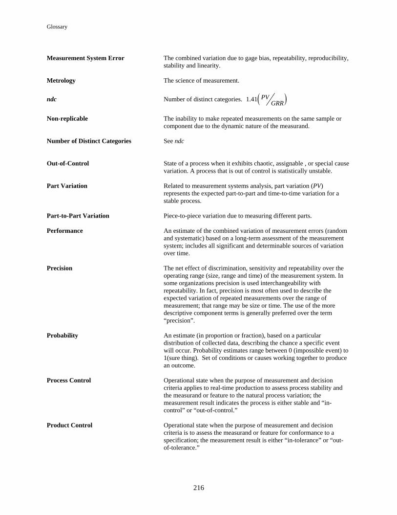
Glossary
216
Measurement System Error The combined variation due to gage bias, repeatability, reproducibility,
stability and linearity. Metrology The science of measurement.
ndc Number of distinct categories. 1.41 PVGRR
Non-replicable The inability to make repeated measurements on the same sample or
component due to the dynamic nature of the measurand. Number of Distinct Categories See ndc Out-of-Control State of a process when it exhibits chaotic, assignable , or special cause
variation. A process that is out of control is statistically unstable. Part Variation Related to measurement systems analysis, part variation (PV)
represents the expected part-to-part and time-to-time variation for a stable process.
Part-to-Part Variation Piece-to-piece variation due to measuring different parts. Performance An estimate of the combined variation of measurement errors (random
and systematic) based on a long-term assessment of the measurement system; includes all significant and determinable sources of variation over time.
Precision The net effect of discrimination, sensitivity and repeatability over the
operating range (size, range and time) of the measurement system. In some organizations precision is used interchangeability with repeatability. In fact, precision is most often used to describe the expected variation of repeated measurements over the range of measurement; that range may be size or time. The use of the more descriptive component terms is generally preferred over the term “precision”.
Probability An estimate (in proportion or fraction), based on a particular
distribution of collected data, describing the chance a specific event will occur. Probability estimates range between 0 (impossible event) to 1(sure thing). Set of conditions or causes working together to produce an outcome.
Process Control Operational state when the purpose of measurement and decision
criteria applies to real-time production to assess process stability and the measurand or feature to the natural process variation; the measurement result indicates the process is either stable and “in-control” or “out-of-control.”
Product Control Operational state when the purpose of measurement and decision
criteria is to assess the measurand or feature for conformance to a specification; the measurement result is either “in-tolerance” or “out-of-tolerance.”
Glossary
217
Reference Value A measurand value that is recognized and serves as an agreed upon reference or master value for comparison:
A theoretical or established value based on scientific principles;
An assigned value based on some national or international organization;
A consensus value based on collaborative experimental work under the auspices of a scientific or engineering group; or
For a specific application, an agreed upon value obtained using an accepted reference method.
A value consistent with the definition of a specific quantity and accepted, sometimes by convention, as appropriate for a given purpose.
NOTE: Other terms used synonymously with reference value
accepted reference value accepted value conventional value conventional true value assigned value best estimate of the value master value master measurement
Regression Analysis A statistical study of the relationship between two or more variables. A
calculation to define the mathematical relationship between two or more variables.
Repeatability The common cause, random variation resulting from successive trials
under defined conditions of measurement. Often referred to as equipment variation (EV), although this is misleading. The best term for repeatability is within-system variation when the conditions of measurement are fixed and defined – fixed part, instrument, standard, method, operator, environment, and assumptions. In addition to within-equipment variation, repeatability will include all within variation from the conditions in the measurement error model.
Replicable The ability to make repeated measurements on the same sample or
component where there is no significant physical change to the measurand or measurement environment.
Replication Multiple test trials under repeatable (identical) conditions. Reproducibility The variation in the average of measurements caused by a normal
condition(s) of change in the measurement process. Typically, it has been defined as the variation in average measurements of the same part (measurand) between different appraisers (operators) using the same measuring instrument and method in a stable environment. This is often true for manual instruments influenced by the skill of the operator. It is not true, however, for measurement processes (i.e., automated systems) where the operator is not a major source of variation. For this reason, reproducibility is referred to as the average variation between-systems or between-conditions of measurement.
Glossary
218
Resolution May apply to measurement resolution or effective resolution The capability of the measurement system to detect and faithfully
indicate even small changes of the measured characteristic. (See also discrimination.)
The resolution of a measurement system is if there is an equal probability that the indicated value of any part which differs from a reference part by less than will be the same as the indicated value of the reference part. The resolution of a measurement system is impacted by the measurement instrument as well as other sources of variation of the total measurement system.
Scatter Diagram A X-Y plot of data to assess the relationship between two variables. Sensitivity Smallest input signal that results in a detectable (discernable) output
signal for a measurement device. An instrument should be at least as sensitive as its unit of discrimination. Sensitivity is determined by inherent gage design and quality, in-service maintenance, and operating condition. Sensitivity is reported in units of measurement.
Significance level A statistical level selected to test the probability of random outcomes;
also associated with the risk, expressed as the alpha ( ) risk, that represents the probability of a decision error.
Stability The absence of special causes of variation; the property of being in
statistical control. Refers to both statistical stability of a measurement process and measurement stability over time. Both are vital for a measurement system to be adequate for its intended purpose. Statistical stability implies a predictable, underlying measurement process operating within common cause variation (in-control). Measurement stability (alias drift) addresses the necessary conformance to the measurement standard or reference over the operating life (time) of the measurement system.
Tolerance Allowable deviation from a standard or nominal value that maintains
fit, form, and function. See also Specification
Uncertainty A parameter associated with the result of a measurement that
characterizes the dispersion of the values that could reasonably be attributed to the measurand (VIM); the range assigned to a measurement result that describes, within a defined level of confidence, the limits expected to contain the true measurement result. Uncertainty is a quantified expression of measurement reliability.
Unimodal A contiguous group of data (distribution) that has one mode

Reference List
219
Reference List
1. ASTM E691-99, Standard Practice for Conducting an Interlaboratory Study to Determine the Precision of a Test Method, (www.astm.org).
2. ASTM E177-90a, Standard Practice for Use of the Terms Precision and Bias in ASTM Test Method, (www.astm.org).
3. ASTM E456-96, Standard Terminology for Relating to Quality and Statistics, (www.astm.org).
4. AT&T Statistical Quality Control Handbook, Delmar Printing Company, Charlotte, NC, 1984.
5. Baker, E. “Signal Detection Theory of Quality Control Inspector Performance”, Journal of Quality Technology, Vol. 7, No.2, April 1975.
6. Bland, J. M., and Altman, D. G. (1986). Statistical methods for assessing agreement between two methods of clinical measurement. Lancet i, pp. 307–310.
7. Burdick, Richard K., and Larsen, Greg A., “Confidence Intervals on Measures of Variability in R&R Studies,” Journal of Quality Technology, Vol. 29, No. 3, July 1997.
8. Cohen, J. (1960) "A coefficient for agreement for nominal scales" in Education and Psychological Measurement. Vol. 20, pp. 37–46.
9. Dataplot, National Institute of Standards and Technology, Statistical Engineering Division, (www.itl.nist.gov).
10. Deming, W. E., Out of the Crisis, Massachusetts Institute of Technology, 1982, 1986.
11. Deming, W. E., The New Economics for Industry, Government, Education, The MIT Press, 1994, 2000.
12. Duncan, A. J., Quality Control and Industrial Statistics, 5th ed., Richard D. Irwin, Inc., Homewood, Illinois, 1986.
13. Eagle, A. R., “A Method For Handling Errors in Testing and Measuring,” Industrial Quality Control, March, 1954, pp. 10-14.
14. Ermer, Donald S., and E-Hok, Robin Yang, “Reliable Data is an Important Commodity,” University of Wisconsin, Madison; published in The Standard, ASQ Newsletter of the Measurement Quality Division, Vol. 97-1, Winter 1997.
15. Everitt, B. (1996) Making Sense of Statistics in Psychology (Oxford University Press).
16. Fleiss, J. L. (1971) "Measuring nominal scale agreement among many raters" in Psychological Bulletin. Vol. 76, No. 5, pp. 378–382.
17. Foster, Lowell W., GEO-METRICS: The Metric Application of Geometric Tolerancing, Addison-Wesley Publishing Company, Reading, Massachusetts, 1993.
Reference List
220
18. Gillespie, Richard, A History of the Hawthorne Experiments, Cambridge University Press, New York, 1991.
19. Grubbs, F. E., “On Estimating Precision of Measuring Instruments and Product Variability,” Journal of the American Statistical Association, Vol. 43, 1948, pp.243-264.
20. Grubbs, F. E., “Errors of Measurement, Precision, Accuracy and the Statistical Comparison of Measuring Instruments,” Technometrics, Vol. 15, February 1973, pp. 53-66.
21. Gruska, G. F., and Heaphy, M. S., “Measurement Systems Analysis,” TMI Conference Workshop, Detroit, Michigan, 1987.
22. Guide to the Expression of Uncertainty in Measurement, ISO/IEC Guide 98:1995.
23. Hahn, J. H. and Nelson, W., “A Problem in the Statistical Comparison of Measuring Devices,” Technometrics, Vol. 12., No. 1, February 1970, pp. 95-102.
24. Hamada, Michael, and Weerahandi, Sam, “Measurement System Assessment Via Generalized Inference,” Journal of Quality Technology, Vol. 32, No. 3, July 2000.
25. Hayes, A. F. & Krippendorff, K. (2007). Answering the call for a standard reliability measure for coding data. Communication Methods and Measures, 1, 77-89.
26. Heaphy, M. S., et. al., “Measurement System Parameters,” Society of Manufacturing Engineering -IQ81-154, Detroit, Michigan, 1981.
27. Hicks, Charles R.and Turner K.V. Jr. Fundamental Concepts in the Design of Experiments, Oxford University Press, New York, 1999.
28. International Vocabulary of Basic and General Terms in Metrology (abbr. VIM), ISO/IEC Guide 99:2007.
29. Ishikawa, Kaoru, Guide to Quality Control, Asian Productivity Organization, 1986.
30. Jaech, J. L., “Further Tests of Significance for Grubbs’ Estimators,” Biometrics, 27, December, 1971, pp. 1097-1101.
31. James, P. D., “Graphical Displays of Gage R&R Data,” AQC Transaction, ASQC, 1991.
32. Krippendorff, K. (2004). Content analysis: An introduction to its methodology. Thousand Oaks, CA: Sage. pp. 219-250.
33. Lipson, C., and Sheth, N. J., Statistical Design & Analysis of Engineering Experiment, McGraw-Hill, New York, 1973.
34. Maloney, C. J., and Rostogi, S. C., “Significance Test for Grubbs’ Estimators,” Biometrics, 26, December, 1970. pp. 671-676.
35. Mandel, J., “Repeatability and Reproducibility,” Journal of Quality Technology, Vol.4, No.2, April, 1972, pp.74-85.

Reference List
221
36. McCaslin, J. A., and Gruska, G. F., “Analysis of Attribute Gage Systems,” ASQC Technical Conference Transactions, 1976, pp. 392-399.
37. Measurement Systems Analysis Reference Manual, Third Edition, Chrysler, Ford, GM, Third Printing, 2002.
38. Minitab User’s Guide: Guide to Minitab: Release 15 - Minitab , Minitab, Inc., 2007.
39. Montgomery, Douglas C., and Runger, George C., “Gauge Capability and Designed Experiments. Part I: Basic Methods; Part II: Experimental Design Models and Variance Component Estimation,” Quality Engineering, Marcel Dekker, Inc., 1993.
40. Nelson, L., “Use of the Range to Estimate Variability,” Journal of Quality Technology, Vol. 7, No.1, January, 1975, pp.46-48.
41. Potential Failure Mode and Effects Analysis (FMEA) Reference Manual, Fourth Edition, DaimlerChrysler, Ford, GM, 2008.
42. Production Part Approval Process (PPAP), Fourth Edition, DaimlerChrysler, Ford, GM, 2008.
43. Saal, F.E., Downey, R.G. and Lahey, M.A (1980) "Rating the Ratings: Assessing the Psychometric Quality of Rating Data" in Psychological Bulletin. Vol. 88, No. 2, pp. 413–428.
44. Shrout, P. and Fleiss, J. L. (1979) "Intraclass correlation: uses in assessing rater reliability" in Psychological Bulletin. Vol. 86, No. 2, pp. 420–428.
45. Spiers, Beryl, “Analysis of Destructive Measuring Systems,” ASQC Quality Congress Transactions, Toronto, 1989.
46. Statistical Process Control Reference Manual (SPC), Second Edition, Chrysler, Ford, GM, 2005.
47. Thompson, W. A., Jr., “The Problem of Negative Estimates of Variance Components,” Annals of Mathematical Statistics, No. 33, 1962, pp. 273-289.
48. Thompson, W. A., Jr., “Precision of Simultaneous Measurement Procedures”, American Statistical Association Journal, June, 1963, pp. 474-479.
49. Traver, R. W., “Measuring Equipment Repeatability – The Rubber Ruler,” 1962 ASQC Convention Transactions, pp. 25-32.
50. Tsai, Pingfang, “Variable Gauge Repeatability and Reproducibility Study Using the Analysis of Variance Method,” Quality Engineering, Marcel Dekker, Inc., 1988.
51. Uebersax, John S. (1987). "Diversity of decision making models and the measurement of interrater agreement" in Psychological Bulletin. Vol 101, pp. 140–146.
52. Vardeman, Stephen B., and VanValkenburg, Enid S., “Two-Way Random-Effects Analyses and Gauge R&R Studies,” Technometrics, Vol. 41, No. 3, August 1999.
53. Wheeler, D. J., “Evaluating the Measurement Process When the Testing is Destructive,” TAPPI, 1990 Polymers Lamination & Coatings Conference Proceedings, (www.tappi.org search for document plc90805).

Reference List
222
54. Wheeler, D. J., and Lyday, R. W., Evaluating the Measurement Process, SPC Press, Inc., Knoxville, Tennessee, 2006 .
223
Sample Forms
The reader has permission to reproduce the forms in this section for internal use only, not for commercial use or resale.
The forms in this section each represent a possible format for GRR data collection and reporting.
They are not mutually exclusive to other types of formats which may contain the same information and accomplish the same results.

224
Gage Repeatability and Reproducibility Data Collection Sheet
PART
Appraiser /Trial # 1 2 3 4 5 6 7 8 9 10
AVERAGE
A 1
2
3
Average aX =
Range aR =
B 1
2
3
Average bX =
Range bR =
C 1
2
3
Average cX =
Range cR =
Part Average
X =
pR =
([ aR = ] + [ bR = ] + [ cR = ]) / [ # OF APPRAISERS = ] = R =
DIFF
X [Max X = ] - [Min X = ] = DIFFX =
*R 4
UCL [R = ] [D ] = =
*D4 = 3.27 for 2 trials and 2.58 for 3 trials. UCLR represents the limit of individual R’s. Circle those that are
beyond this limit. Identify the cause and correct. Repeat these readings using the same appraiser and unit as originally used or
discard values and re-average and recompute R and the limiting value from the remaining observations.
Notes:_____________________________________________________________________________________________________________

225
Gage Repeatability and Reproducibility Report
Part No. & Name: Characteristics: Specifications:
From data sheet: R =
Gage Name: Gage No: Gage Type:
DIFFX =
Date: Performed by:
pR =
Measurement Unit Analysis % Total Variation (TV)
Repeatability – Equipment Variation (EV)
EV = R K1 Trials K1 %EV = 100 [EV/TV]
= _______ _______ 2 0.8862 = 100 [_______/_______]
= _______ 3 0.5908 = _______%
Reproducibility – Appraiser Variation (AV)
AV = 2 2
2 ( ( ))-DIFFX K EV nr %AV = 100 [AV/TV]
= 2 2_____ _____ ( _____ (__ __) )- = 100 [_______/_______]
= _______ Appraisers 2 3 = _______%
n = parts r = trials K2 0.7071 0.5231
Repeatability & Reproducibility (GRR)
GRR = 2 2 EV AV
%GRR= 100 [GRR/TV]
= 2 2_____ _____ Parts K3 = 100 [_______/_______]
= _______ 2 0.7071 = _______%
Part Variation (PV) 3 0.5231
PV = pR K3 4 0.4467 % PV = 100 [PV/TV]
= _______ _______ 5 0.4030 = 100 [_______/_______]
= _______ 6 0.3742 = _______%
Total Variation (TV) 7 0.3534
TV = 2 2 GRR PV 8 0.3375 ndc = 1.41 PVGRR
= 2 2_____ _____ 9 0.3249 = 1.41(_______/_______)
= _______ 10 0.3146 = _______
For information on the theory and constants used in the form see MSA Reference Manual, Fourth edition.

226

Index
227
Index

Index
228
Acceptability Criteria, 79 Accuracy (also see Bias), 6, 50, 215, 222 Analysis Of Variance (ANOVA), 103, 105, 109, 125,
126, 127, 128, 129, 130, 131, 161, 163, 165, 169, 197, 199, 200, 212, 215
Analytic Method, 147 Apparent, 215 Appraiser Variation (AV), 7, 122, 124, 125, 129, 131,
197, 198, 200, 209, 215, 227 ASTM (American Society For Testing And Materials),
5, 6, 7, 33, 45, 50, 54, 55, 56, 187, 189, 192, 221 Attribute, 133, 136, 147, 151, 152, 161, 179, 181,
223 Average, 95, 103, 105, 108, 109, 114, 115, 119, 126,
128, 129, 130, 131, 171, 176, 177, 188, 226 Bias, 6, 50, 51, 61, 62, 89, 90, 91, 92, 93, 94, 96, 97,
99, 215, 221 Calibration, 10, 34, 36, 38, 39, 43, 213, 215, 216 Calibration Standard, 43 Capability Index, 201 Cause and Effect, 17, 68 Cause and Effect Diagram, 17, 68 Charts, Error, 114 Check Standard, 45 Consistency, 8, 57, 110, 112, 113, 116, 166, 187, 192 Control Chart Analysis, 88 Control Charts, 49 Coordinate Measuring Machine (CMM), 14, 25, 26,
37, 38, 59, 134, 169, 213 Cp (see Capability Index), 21, 22, 143, 201, 203, 204 Cross‐tabulation, 135 Customer, 4, 48, 91, 96, 233 Designed Experiment, 216, 223 Destructive measurement systems, 155, 156
impact testing (gravelometer), 155 mass spectroscopy, 155 material characteristic testing, 155 plating testing, 155 salt spray/humidity booth testing, 155 weld testing, 155
Discrimination, 5, 41, 46, 216 Drift (see Stability), 6, 39 Effective Resolution, 38, 216 Effectiveness, 141, 142 Environment, 16, 37, 51, 54, 211 Equipment Variation (EV) (see also Repeatability),
227 Ergonomics, 38 Error, 19, 39, 79, 80, 97, 114, 115, 182, 209, 211,
213, 218
Error Charts, 114 Error Rate, 19 EV (see Equipment Variation), 54, 90, 93, 95, 99,
122, 124, 125, 129, 131, 197, 198, 200, 209, 219, 227
False Alarm Rate, 19, 142 Fixturing, 37 FMEA, 13, 26, 37, 169, 223 Gage, 5, 7, 31, 35, 42, 56, 61, 79, 81, 90, 103, 105,
107, 118, 121, 122, 125, 131, 147, 148, 150, 151, 152, 161, 179, 180, 181, 182, 183, 184, 198, 207, 211, 212, 213, 217, 222, 223, 226, 227
Gage Performance Curve (GPC), 42, 147, 148, 150, 151, 152, 179, 180, 181, 182, 183, 184
Gage Repeatability (GR), 35, 107, 118, 120, 121, 122, 125, 226, 227
Gage Repeatability and Reproducibility (GRR), 7, 56, 107, 118, 121, 122, 125, 161, 198, 212, 217, 222, 226, 227
Geometric Dimensioning and Tolerancing (GD&T), 169
GPC (see Gage Performance Curve), 42, 148, 150, 179, 181
GRR (see Gage Repeatability and Reproducibility), 7, 18, 22, 35, 56, 58, 60, 64, 75, 76, 79, 80, 81, 90, 95, 99, 104, 105, 106, 122, 123, 124, 125, 129, 130, 131, 145, 146, 150, 163, 165, 181, 185, 186, 187, 189, 193, 197, 198, 199, 200, 201, 202, 203, 212, 216, 217, 225, 227
Guide to the Expression of Uncertainty in Measurement, 222
Histogram, 93, 115, 217 Hypothesis Test Analyses, 133, 135 Kappa, 138, 139, 217 Linearity, 6, 51, 52, 98, 100, 101, 102, 116, 164, 207,
217 Location Error, 79 Maintenance, 34, 36, 38 Master, 44, 213 Measurand, 60, 217 Measurement Life Cycle, 26 Measurement System, 1, 7, 8, 13, 17, 18, 28, 31, 37,
38, 39, 67, 68, 69, 75, 79, 83, 87, 131, 133, 134, 155, 156, 171, 187, 212, 218, 222, 223
Measurement System Performance, 8 Measurement Uncertainty, 63 Miss Rate, 19, 142 NIST (National Institute of Standards and Technology), 9, 159, 221

Index
229
NIST (see National Institute of Standards and Technology), 9, 10, 11, 34, 45, 73
NMI (National Measurements Institute), 9, 10, 45 Non‐replicable, 218 Number of Distinct Categories (ndc), 47, 80, 125,
131, 216, 218, 227 Observed Value, 114, 115 Operational Definition, 43 P.I.S.M.O.E.A., 16, 37, 211 P.I.S.M.O.E.A. Error Model, 211 Performance Curve, 42, 147, 148, 150, 151, 152,
179, 180, 181, 182, 183, 184 Pooled Standard Deviation, 187, 190, 191 Precision, 7, 54, 218, 221, 222, 223 Process Control, 49, 75, 131, 215, 218, 223 Process Failure Mode Effects Analysis (PFMEA), 13 Product Control, 75, 218 R&R (see Gage Repeatability and Reproducibility or GRR), 7, 56, 163, 198, 212, 217, 221, 222, 223
Random, 213, 223 Randomization, 76, 106 Range, 38, 90, 95, 103, 104, 105, 110, 111, 124, 126,
128, 129, 130, 131, 160, 163, 171, 176, 177, 188, 203, 207, 223, 226
Range Chart, 110, 111 Range Method, 90, 104, 105, 128, 131, 163, 171, 188 Reference Value, 45, 92, 101, 114, 115, 145, 219 Replicable, 83, 155, 219 Reproducibility, 7, 55, 77, 103, 107, 118, 121, 122,
125, 131, 189, 198, 207, 215, 219, 222, 223, 226, 227
Resolution, 38, 215, 216, 220 Resolution, Apparent, 215
Resolution, Effective, 38, 216 Risk Analysis Methods, 133 Rule of Tens, 15, 41 Run Chart, 111 S.W.I.P.E., 16, 37 Scatter Plot, 112 Sensitivity, 8, 38, 57, 220 Signal Detection Approach, 145 Standard, 5, 16, 43, 44, 45, 105, 163, 165, 176, 177,
187, 190, 191, 198, 209, 211, 213, 221 Standard, Calibration, 43 Standard, Check, 45 Standard, Reference, 43 Standard, Transfer, 44 Standard, Working, 44 Statistical Process Control (SPC), 11, 47, 49, 75, 79,
88, 118, 213, 215, 223, 224 Test Stands, 155, 156, 161 Tolerance, 124, 131, 145, 203, 220 Total Variation (TV), 15, 76, 90, 95, 99, 119, 123,
124, 125, 129, 131, 200, 227 Traceability, 9, 10, 64 Transfer Standard, 44 True Value, 45 Uncertainty (see Measurement Uncertainty), 8, 60,
63, 64, 65, 220, 222 Uniformity, 8, 58 Variable Gage Study, 103 Variation, 7, 15, 50, 76, 103, 119, 123, 124, 129, 131,
169, 185, 198, 200, 215, 218, 227 Whiskers Chart, 113 Width Error, 79, 80 Working Standard, 44

230
Feedback
231
M.S.A. Manual User Feedback Process
Consistent with the concept of continual improvement, this automotive industry measurement systems analysis (MSA) manual is being subjected to a formal periodic review/revision process. In line with the concept of customer satisfaction, this review will entail consideration of not only any applicable vehicle manufacturer requirement changes from year to year but also of feedback from users of the manual for the purpose of making it more value-added and effective to the automotive industry and user communities. Accordingly, please feel free to offer, in writing, your feedback comments, both pro and con, relative to the manual’s understandability, “user-friendliness,” etc., in the area indicated below. Please indicate specific manual page numbers where appropriate. Forward your feedback to the address indicated below: Your Name _____________________________________________________ Representing ________________________________________________ Company/Division Name Address _____________________________________________________ _____________________________________________________ _____________________________________________________ Phone ___(____)________________ Please list your top three automotive customers and their locations. ________________________ ________________________ Customer Location ________________________ ________________________ Customer Location ________________________ ________________________ Customer Location Feedback Comments (attach additional sheets if needed)
_____________________________________________________ _____________________________________________________ _____________________________________________________ _____________________________________________________ _____________________________________________________ Send Comments To: Automotive Industry Action Group Suite 200 26200 Lahser Road Southfield, Michigan 48033 MSA, 4th Please access www.aiag.org to submit your feedback electronically.
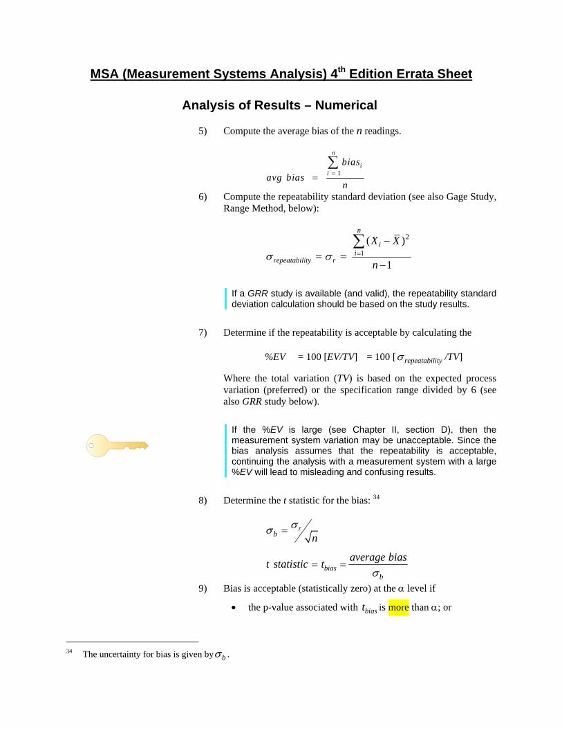
MSA (Measurement Systems Analysis) 4th Edition Errata Sheet
Analysis of Results – Numerical
5) Compute the average bias of the n readings.
1
n
ii
bias
avg biasn
==∑
6) Compute the repeatability standard deviation (see also Gage Study, Range Method, below):
2
1
( )
1
n
ii
repeatability r
X X
nσ σ =
−= =
−
∑
If a GRR study is available (and valid), the repeatability standard deviation calculation should be based on the study results.
7) Determine if the repeatability is acceptable by calculating the
%EV = 100 [EV/TV] = 100 [ repeatabilityσ /TV]
Where the total variation (TV) is based on the expected process variation (preferred) or the specification range divided by 6 (see also GRR study below).
If the %EV is large (see Chapter II, section D), then the measurement system variation may be unacceptable. Since the bias analysis assumes that the repeatability is acceptable, continuing the analysis with a measurement system with a large %EV will lead to misleading and confusing results.
8) Determine the t statistic for the bias: 34
rb n= σσ
biasb
average biast statistic t
σ= =
9) Bias is acceptable (statistically zero) at the α level if
• the p-value associated with biast is more than α; or
b34 The uncertainty for bias is given byσ .