1

Measurement of void fraction in dispersed bubbly flow containing micro-bubbles with constant electric current method Shin-ichiro Uesawa, Akiko Kaneko, and Yutaka Abe University of Tsukuba, Graduate School of Systems and Information Engineering Tennodai 1-1-1, Tsukuba-shi, Ibaraki, 305-8573 Japan Abstract

Void fraction is one of the dominant parameter of gas-liquid two-phase flow in industrial equipment. An electric sensing method based on the difference of electric conductivity and permittivity between liquid and gas is one of online measurement methods of void faction. However, previous constant electric current method is not applicable to dispersed bubbly flow because bubbles are dispersed in three dimensions. In the present study, new constant electric current method available to the three dimensional dispersed bubbly flow with tiny bubbles (micro-bubbles) is developed. The proposed method to estimate the void fraction is based on Maxwell’s theory and polarization of tiny bubbles. The method makes it possible to measure the void fraction of three dimensional dispersed bubbly flow. It is experimentally clarified that the present proposed method with constant electric current method can be applicable to measure the void fraction of three dimensional bubbly flow more accurately than previous constant electric current method. It is also clarified that the Maxwell’s theory and the present proposed method with polarization are compatible with drift flux model although void fraction estimated with the previous method is higher than the drift flux model for three dimensional dispersed bubbly flow. Keywords: Void fraction, Micro-bubble, Gas-liquid Two-phase flow, Three-dimensional flow, Constant electrical current method

1. Introduction

Volumetric void fraction is defined as a volumetric ratio in gas phase of gas-liquid two phase flow. It is one of the very important physical values and key parameters in two-phase flow for designs and performance evaluations of devices. Numerous measurement techniques of the void fraction have been developed, such as quick shut valve methods, image processing methods, X-ray CT scan methods, neutron radiography methods, gamma-ray method, NMR and so on [1-9]. They are used to measure void fraction in two-phase flow. However, these measurement methods are subjected to various restrictions. The quick shut valve method is highly accurate for average void fraction, but it is necessary to stop the flow. X-ray CT scan methods, neutron radiography methods, gamma-ray method and NMR can reconstruct three dimensional void distribution, but they need large facility, much cost and time to reconstruct the value of void fraction. It is very difficult to apply those methods to follow highly temporal fluctuations of void fraction as simple systems. On the other hand, electric sensing techniques can realize the online measurement with simple systems. The techniques are based on the difference of electric resistivity or electric permittivity between gas and liquid phase [10-30]. That is, the electric resistance or the capacitance is corresponding to the void fraction in a measuring section. There are all kinds of electric sensing methods such as conductance proves methods [10-13], wire mesh methods [14-16], electric resistance tomography (ERT) [17, 18], capacitance method [19-24], electric capacitance tomography (ECT) [25] and electric capacitance volume tomography (ECVT) [26]. These electric sensing methods need large systems required complex algorism to reconstruct void value and they need large reconstructing time to obtain the void value. On the other hand, one of the electric sensing method proposed by Fukano (1998) [27] is simple and quick response to temporal void fluctuation. In previous study, the method was applied to measure the void fraction in

2

two dimensional annular flow. The method was used to measure the void fraction in annular flow and liquid film thickness [27-30].

In this method, a constant electrical current DC power supply applies to gas-liquid two-phase flow through a pair of electrodes which are mounted flush with a surface of a channel. These electrodes are named “applied electrodes”. A voltage is measured with a voltage drop method by using another pair of electrodes which are set between the applied electrodes. These electrodes are named “measuring electrodes”. Characteristics of the constant electrical current method are as follows. Applied electrodes are separated from measuring electrodes and two measuring electrodes are set between two applied electrodes. By this arrangement of electrodes, the electrical current density applied by the constant current power supply becomes satisfactory uniform in the measuring section. The voltage drop is picked-up through high impedance, then the uniform electrical current distribution is not disturbed with the presence of the pair of measuring electrodes, and interaction among measuring electrodes is negligible. Therefore a number of measuring electrodes can be set in a short distance [27, 28].

The objective of the present study is to evaluate the void fraction of three dimensional bubbly flow containing micro-bubbles by using the constant electric current method. Tiny bubbles in diameter of 1 μm to 1 mm which are called micro-bubbles are applied in many subjects in engineering fields, such as water purification systems, frictional drag reductions of ships, medical technologies, and so on [31]. In addition, micro-bubbles have been also applied as tracer particles for Ultrasonic Doppler Methods which are used for velocity measurements [32]. Thus a void fraction meter which has high spatial resolution is required to measure tiny bubbles.

The existing constant electric current method is applied to two dimensional annular flow based on the assumption that the cross-section ratio between gas and liquid is constant in flow direction. The method is simple, low cost, easy handling and quick response. However, the method cannot be applied to three dimensional bubbly flow because the existing algorithm cannot treat the bubbles distributed in three dimensions. In previous studies, Maxwell’s theory [33] was applied to bubbly flow for calculations of void fraction from electric signals by using probes [10, 22] and an electric resistance tomography [18]. However, the theory is not applied to the constant electric current method. The purpose of the present study is to apply constant electric current method to measure the three dimensional dispersed bubbly flow. In order to achieve the purpose, Maxwell’s theory and new concept to estimate the electric signal to void fraction for three dimensional dispersed bubbly flow are introduced in the present study.

2. Calculation methods of void fraction

2.1. Previous method A calculation method of the void fraction in the constant electrical current method is based on a cross-sectional

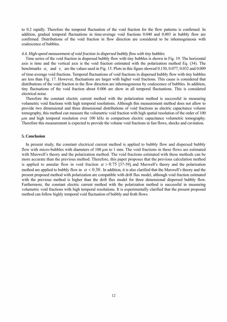
area of liquid between measuring electrodes [27]. The calculation model is shown in Fig. 1. The cross-sectional area of liquid is assumed to be a plate electrode. The electrical resistance of gas-liquid two phase flow R′ is

LL S

LR ρ′=′ (1)

where Lρ′ is an electrical resistivity of liquid, L is a length between measuring electrodes and LS is a cross-sectional area of

liquid. On the other hand, resistance of liquid single phase flow 0R′ is

3

00 S

LR Lρ′=′ (2)

where 0S is a total cross-sectional area. A volumetric void fraction α is defined as

0

0

VVV L−

=α (3)

where 0V is a total volume and LV is a volume of liquid. If the cross-sectional area of liquid is constant

between measuring electrodes, the volumetric void fraction is

LSLSLS L

0

0 −=α . (4)

From Eqs. (1) and (2), the volumetric void fraction between measuring electrodes is

RIRI

′′′′

−= 01α . (5)

I ′ is a constant electrical current. The void fraction is shown with measured voltages of gas-liquid two-phase

flow and liquid single phase flow V ′ and 0V ′ .

VVV′

′−′= 0α . (6)

The following equation is obtained by normalizing for measured voltage of liquid single flow 0V ′ .

vv

′−′

=1α (7)

where ( )0VVv ′′≡′ is a voltage ratio.

The void fraction α is calculated from electrical voltage ratio v′ as above. This method is applied to annular flow because the cross-sectional area of liquid is assumed to be constant between electrodes. However, because bubbles are dispersed in three dimensions in bubbly flow, liner relationship between the voltage and the cross-sectional area of liquid is not obtained and the void fraction in bubbly flow cannot be estimated accurately from Eq. (7).

4

2.2. Maxwell’s theory Maxwell calculated a resistance of a mixture of two mediums which had different resistivity each other [33]. In

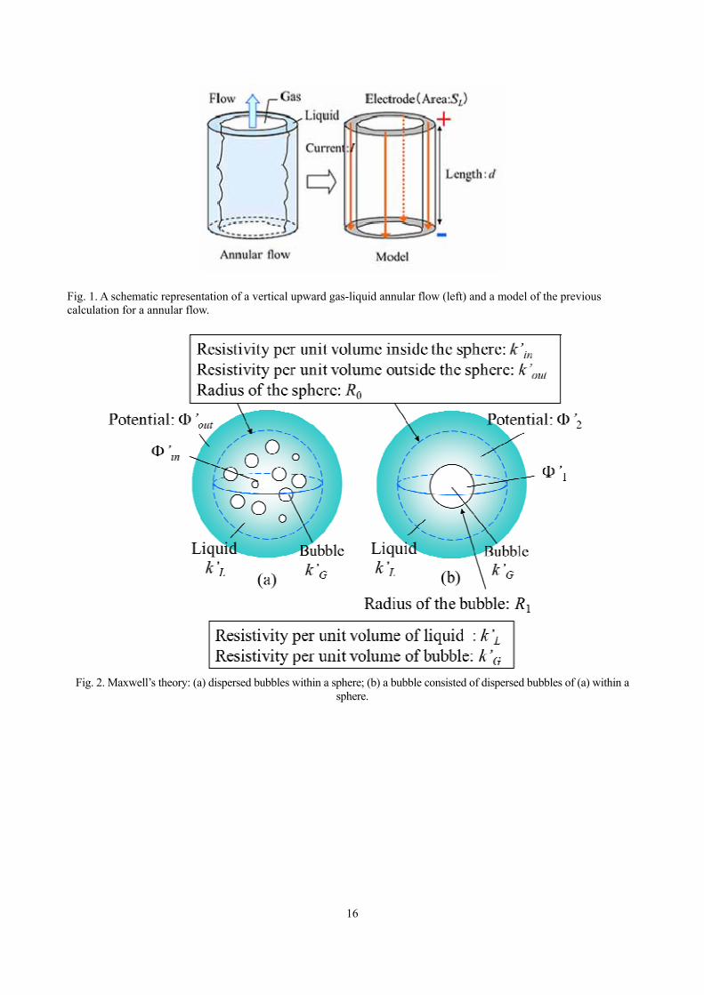
the preset study, this calculation method is applied to constant electrical current method. Two mediums are assumed to be gas and liquid in this model. The calculation model is shown in Fig. 2. Dash lines in the figure (a) and (b) show spheres with radius of 0R . Physical quantities inside and outside spheres are noted “in” and “out” as subscripts, and physical quantities of gas and liquid are noted “G” and “L” as subscripts. k ′ is a resistivity per unit volume. The model of dispersed bubble (a) is discussed at first. The potential inside and outside the sphere is calculated. The resistivity of these bubbles is Gk′ . It is assumed that bubbles do not existed and liquid is filled outside the sphere. Hence the resistivity outside the sphere outk′ is equivalent to the resistivity of liquid Lk′ . A potential of electrical dipole Φ′ is assumed to apply inside and outside the sphere. From Laplace equation, the potential of the electrical dipole Φ′ is

02 =Φ′∇ (8)

and

( ) ( ) 01

2 YBrArr −+=Φ′ (9)

where A and B are constant numbers, r is a radial coordinate from the center of the sphere and 0

1Y is a spherical surface harmonics. The potential and the current are conserved at the boundary of the sphere, 0Rr = .

( ) ( )00 RR outin Φ′=Φ′ (10)

and

020

11

Rdrd

kRdrd

koutin

in

⎟⎠⎞

⎜⎝⎛ Φ′

′=⎟

⎠⎞

⎜⎝⎛ Φ′

′. (11)

Equation (9) is substituted for Eqs. (10) and (11) of boundary conditions.

( ) ( )30

30

322

RkBkkRAkkA

in

inLininLinout ′

′−′+′+′= (12)

and

( ) ( )in

inLininLinout k

BkkRAkkB′

′+′+′−′=

3

30 . (13)

When an electrical source and a sink are not existed in the sphere, ∞→Φ′in is unsatisfied with 0→r , and

0=inB is obtained from Eq. (9). From Eqs. (12) and (13),

5

( )out

Lin

Linout A

kkRkkB′+′

′−′=

2

30 (14)

is obtained. The potential outside the sphere is

( ) ( ) 01

230

2YAr

kkRkk

rr outLin

Linout ⎥

⎦

⎤⎢⎣

⎡′+′

′−′+=Φ′ − . (15)

In the right figure (b) of Fig. 2, dispersed bubbles are gathered to the center, then a spherical bubble consists of

these bubbles. The radius of the sphere and the spherical bubble are 0R and 1R . The center of the sphere and the bubble are placed on the origin of the spherical coordinate. The potential of the dipole inside the bubble is

1Φ′ , and the potential outside the bubble is 2Φ′ . The potential and the current in the boundary of the bubble are conserved.

( ) ( )1211 RR Φ′=Φ′ (16)

and

1

2

1

1 11

Rdrd

kRdrd

k LG

⎟⎠⎞

⎜⎝⎛ Φ′

′=⎟

⎠⎞

⎜⎝⎛ Φ′

′. (17)

As above calculation, 2Φ′ is

( ) ( ) 012

231

2 2YAr

kkRkkrrLG

LG⎥⎦

⎤⎢⎣

⎡′+′

′−′+=Φ′ − . (18)

Then 2Φ′=Φ′out is assumed when Rr > . The assumption shows that the potential without the sphere included dispersed bubbles and the sphere included the single spherical bubble are equivalent. In addition, Ar≅Φ′ is obtained from 2−>> BrAr when r is large, then 2AAout = . From these assumptions, the resistivity within the sphere included dispersed bubbles ink′ is

( ) ( )

( ) 30

31

30

31

22

2

RRkkkk

kkkRRkkk

kLGLG

LGLLGL

in

′−′+′−′−

′+′′−′−′′−=′ . (19)

If Gk′ is the resistivity of air and Lk′ is the resistivity of water, from LG kk ′>>′

Lin kk ′−

+=′

αα

15.01

. (20)

6

The volumetric void fractionα is

30

31

RR

=α . (21)

α is the volumetric void fraction because the total volume of dispersed bubbles 4/3πR1

3 is divided by the volume of the sphere included dispersed bubbles 4/3π3R0

3. The void fraction α in Eq. (20) is represented as

5.01

+′−′

=vvα . (22)

The void fraction estimated by Maxwell’s theory Eq. (22) is lower than the void fraction estimated by the previous method eq. (7) because 1≥′v . Unlike the previous method, the void fraction α in dispersed bubbly flow is expected to measure by Maxwell’s theory which calculates the resistance of gas-liquid two-phase flow in three dimensions. However, the theory is considered to be applicable when gaps between bubbles are longer than bubble diameters because dispersed bubbles are assumed as a gathered bubble, and the spatial distribution and the electrical interaction of each bubble are negligible. 2.3. Polarization method

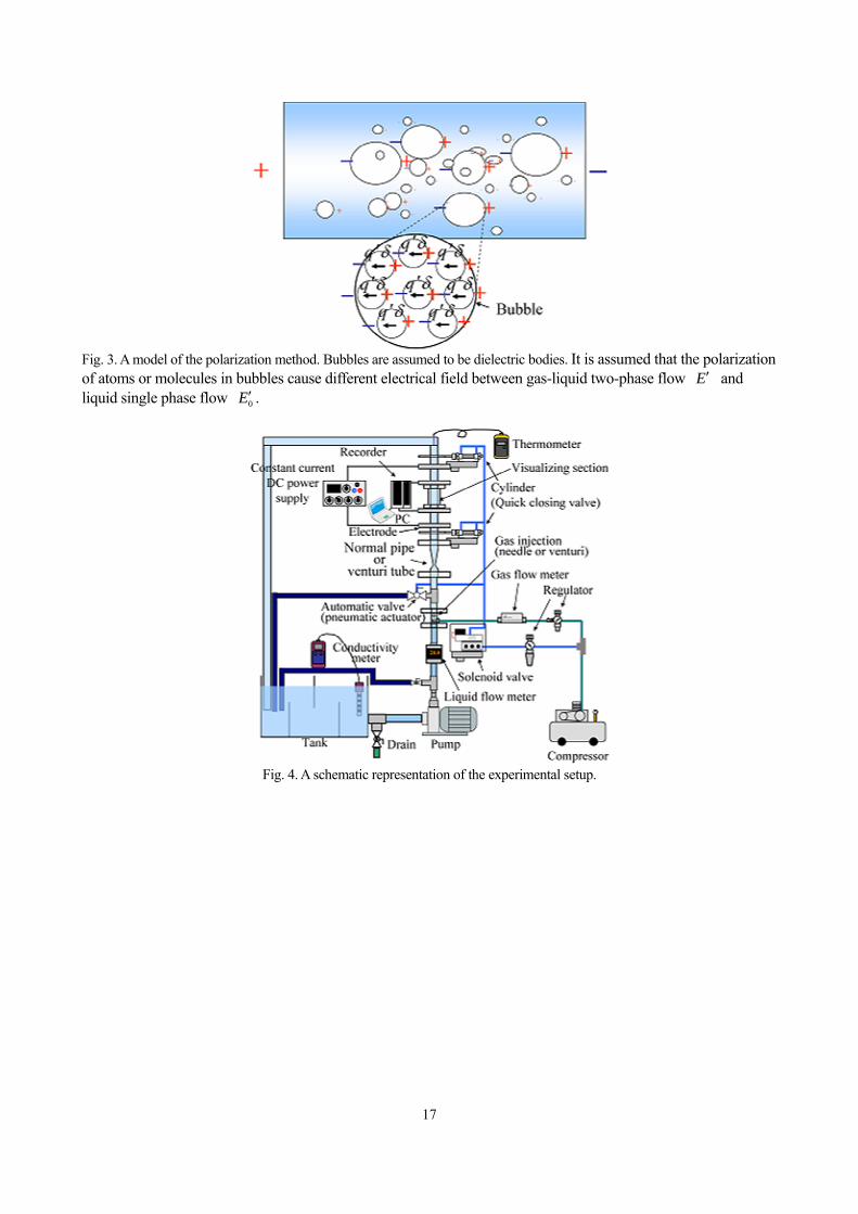
An electrical filed is applied to flow by using electrical measurement methods of void fraction. Then, electrical interactions affect bubbles. In the present study, the calculation method of the void fraction based on difference of electrical field by polarization of bubbles is proposed. The schematic of bubbly flow is shown in Fig. 3. It is assumed that the polarization of atoms or molecules in bubbles cause different electrical field between gas-liquid

two-phase flow E′ and liquid single phase flow 0E′ ,

0EEP ′−′=′′

ε (23)

where P′ is a polarization vector between measuring electrodes and ε ′ is a permittivity, and the field is assumed to be single dimension in the flow direction. The polarization of bubbles P′ is expressed by number of atoms or molecules per

unit of volume of bubbles n , an electrical charge q′ and an interval between positive charges and negative charges δ .

δqnP ′=′ . (24)

A total number of atoms or molecules of bubbles between electrodes N and a total volume of bubbles GV are

totalnVN = (25)

7

and

GG NvV = (26)

where a total volume between measuring electrodes is totalV and the volume of an atom or a molecule of bubbles is Gv .

The void fraction α is defined as

total

G

VV

=α . (27)

From Eqs. (25), (26) and (27), the number of atoms per unit the total volume of bubbles n is

Gvn α

= . (28)

Equations (24) and (28) are substituted to Eq. (23),

0EEvq

G

′−′=′′

εδα . (29)

However, δ and Gv are unknown. For this reason, electrical fields of two difference conditions 1E′ and 2E′ which

are the function of void fractions 1α and 2α are considered from Eq. (29) in order to cancel out these unknown parameters

GvqEE

εδα

′′

=′−′ 101 (30)

and

GvqEE

εδα

′′

=′−′ 202 . (31)

From these equations,

2

1

02

01

αα

=′−′′−′

EEEE

. (32)

8

Electrical fields are approximated as bellow,

10

1

0

1

0

1 vVV

EE ′=

′′

=′Δ′Δ

≅′′

φφ

. (33)

From Eqs. (32) and (33), the volumetric void fraction 2α is

11

22 1

1αα−′−′

=vv

. (34)

From this equation, the void fraction 2α can be obtained from the measured voltage ratio 2v′ , the known void fraction 1α and the known voltage ratio 1v′ . This equation is liner of 2α and 2v′ . This method is applicable under the assumable condition where δ and Gv is constant.

3. Experimental apparatus and conditions

The experimental apparatus in the present study is shown in Fig. 4. It consists of a tank, a pump, a liquid flow meter, a compressor, a gas flow meter, a gas injection and void fraction measurement systems. Tap water filters with 5 μm mesh and air is applied as liquid and gas phases. The void fraction measurement systems consists of an electrical measurement system and a quick shut valve system .

In the electrical measurement system, four ring shaped electrodes are mounted inside of the pipe as shown in Fig.5. These electrodes are made of stainless steel with the width of 10 mm. Two outer electrodes (applied electrodes) are connected to a constant current DC power supply and two inner electrodes (measuring electrodes) are connected to a data logger. The void fraction is estimated with the measuring voltage between two measuring electrodes with voltage drop method. The sampling frequency is 100 kHz and measuring time is 0.5 s. The interval between measuring electrodes is 100 mm, and the interval between the applied electrode and the measuring electrode is 70 mm. The flow path between electrodes is made of acrylic resin which is an insulator. In order to observe flow between measuring electrodes, the test section is made of clear acrylic resin and covers with a water jacket to decrease influence of refraction. The flow is observed with a high-speed video camera and a metal halide lamp.

The void fraction is measured with quick shut valve method in order to compare with the void fraction measured with constant electrical current method. Air cylinders set upstream and downstream are activated with the solenoid valve connected to the compressor, then two slide valves made of stainless steel with thick of 0.5 mm close flow path at the same time. The void fraction is measured with observations of a water level after separation of gas and liquid. The measurement error is 10 % at the maximum for the minimum void fraction. Void fractions are measured 10 times for each experimental condition.

Gas injections with a venturi shape and a needle as shown in Fig. 6 are applied in this experiment. Bubbly flow supplied from the needle with inner diameter of 0.7 mm is discussed in “4.1 Measurement of void fraction in dispersed bubbly flow”. In “4.2 Measurement of void fraction in dispersed bubbly flow with tiny bubbles”, the constant electrical current method measures the void fraction in dispersed bubbly flow with micro-bubbles generated with the venturi shaped gas injection and the venturi tube. The venturi tube is shown in the left figure of Fig. 7. The inner diameter of the inlet and the outlet of the venturi tube is 16 mm, diameter of the throat is 6 mm

9

and the open angle is 6 degrees. Micro-bubbles are generated with the venturi tube as shown in the left figure of Fig. 7 [34]. The interval between the gas injection and the center of the measuring section is 596 mm.

Liquid flow rates 20, 25 and 30 L/min are fixed and gas flow rates are controlled in each liquid flow rates as experimental conditions. Gas flow ratios from 0 to 0.5 L/min are applied in “4.1 Measurement of void fraction in dispersed bubbly flow” and gas flow rates from 0 to 0.2 L/min are applied in “4.2 Measurement of void fraction in dispersed bubbly flow with tiny bubbles”.

Measured voltages are revised with conductivity and temperature of water. The revision with conductivity is

mm VV ′′′

=′0

0 σσ

. (35)

where mV ′ is measured voltage, mσ ′ is measured conductivity, 0σ ′ is a benchmark of conductivity and 0V ′ is revised voltage. The revision with temperature is

( ){ } mmt VttV ′−+=′ 002.01

0 (36)

where mt is temperature when the voltage is measured, 0t is a benchmark of temperature and

0 tV ′ is revised

voltage. 0.02 is temperature correction factor and equivalent to factor of the conductivity meter.

4. Experimental results and discussions

4.1. Measurements of void fraction in dispersed bubbly flow The measurement results of void fractions of bubble supplied from a needle is shown in this section. The

correlation between the voltage ratio obtained with the constant electrical current method v′ and the gas volume flow ratio β is shown in Fig. 8. The voltage ratio is measured the voltage of gas-liquid two-phase flow normalized with the voltage of liquid single phase flow. The gas volume flow ratio is

LG

G

QQQ+

=β (37)

where GQ is a gas flow rate measured by the gas flow meter and LQ is a liquid flow rate measured through the liquid flow meter. The parabolic correlation between the voltage ratio and the gas volume flow ratio is confirmed independently of liquid flow rates in Fig. 8. Measurements of the void fraction in dispersed bubbly flow with the constant electrical current method are expected from this figure.

High-speed video camera images between measuring electrodes with the liquid flow rate 20 L/min are shown in Fig. 9. It is confirmed that bubbly flow changed to froth flow with increasing the gas volume flow ratio. From these results, it is proposed that the void fraction measurement by the constant electrical current method is applicable to bubbly flow and froth flow. Standard deviations of the voltage ratios increase over the gas volume flow ratio 0.2 in Fig.8. It is considered that the void fraction is inhomogeneous in the flow direction because a large bubble and small bubbles inflow to the test section alternately.

The effectiveness method of each calculation of the void fractions from voltage ratios is discussed in order to measure the void fraction in the dispersed bubbly flow. The void fraction measured with the constant electrical current method is compared with the void fraction measured with the quick shut valve method. This result is shown in Fig. 10. The horizontal axis indicates void fractions obtained with the quick shut valve method, the vertical axis indicates void fractions obtained with the constant electrical current method and the dash line shows the equivalent points of both measurements. Error bars of the void fractions measured with the constant electrical

10

current method indicate standard deviations and error bars of the void fraction measured with the quick shut valve method show the maximum and the minimum in the measurement. Benchmarks of voltage ratios and void fractions for the polarization method v1 and α1 are values when error bars of the void fractions measured with the quick shut valve method are minimums for each liquid flow rates.

In Fig. 10, void fractions estimated with each calculation methods are different even if experimental conditions are same. Especially, overestimates of the void fraction are about 110 % at the maximum in the previous calculation method Eq. (7). On the other hand, results of Maxwell’s theory Eq. (22) and polarization method Eq. (34) are coincident with results of quick shut valve method comparatively, and then errors are 40 %. Under low void fractions 0.15, error of the polarization method is about 10 %. It is confirmed that results of the polarization method Eq. (34) proposed in present study are coincident with results of quick shut valve method in comparison to the previous method Eq. (7) and Maxwell’s theory Eq. (22) in low void fractions. These results in each liquid flow rates are not difference under low void fraction 0.15. However, void fractions of Maxwell’s theory Eq. (22) are coincident with void fractions measured with quick shut valve method over high void fraction 0.25 with liquid flow rate 20 L/min. It is made clear that Maxwell’s theory Eq. (22) and the polarization method Eq. (34) are more effective for dispersed bubbly flow than the previous method.

Results compared between calculation methods of the void fraction and drift flux model [35, 36] are shown in Fig. 11 to compare with previous studies. The horizontal axis is the gas volume flux and the vertical axis is void fraction. Plots show void fractions obtained with each calculation methods based on voltage ratios in Fig. 8. The solid line shows the result of drift flux model of bubbly flow in a vertical pipe. In the model, the void fraction α , a distribution parameter 0C and a drift velocity of gas GjV are

GjT

GVjC

j+

=0

α , (38)

L

GCρρ2.02.10 −= (39)

and

( )4/1

22⎪⎭

⎪⎬⎫

⎪⎩

⎪⎨⎧ −

=L

GLGj

gVρ

ρρσ (40)

where Gj is a gas volume flux, Tj is a total volume flux, Gρ is a mass density of gas, Lρ is a mass density of liquid and σ is a surface tension of liquid [35, 36]. In Fig. 11, results of the polarization method are coincident with drift flux model in comparison to previous method Eq. (7) and Maxwell’s theory Eq. (22) with liquid flow rates 20, 25 and 30 L/min. Overestimates of the void fraction are about 150 % at the maximum for the previous method Eq. (7). On the other hand, overestimates are 70 % for Maxwell’s theory Eq. (22) and 50 % for polarization method Eq. (34). It is confirmed that the void fraction obtained with polarization is coincident with drift flux model comparatively.

Therefore, it is made clear from present study that the constant electrical current method is applicable to dispersed bubbly flow by application of Maxwell’s theory Eq. (22) and the polarization method Eq. (34). 4.2. Measurement of void fraction in dispersed bubbly flow with micro-bubbles

The void fraction in dispersed bubbly flow with micro-bubbles is measured with the constant electrical current method. Tiny bubbles are generated with the micro-bubble generator consisted of the venturi tube. The correlation between the voltage ratios obtains with the constant electrical current method v′ and the gas volume flow ratio β is shown in Fig. 12. The liner relation between the voltage ratio and the gas volume flow ratio is confirmed independently of liquid flow rates. Measurements of the void fraction in dispersed bubbly flow with tiny bubbles by the constant electrical current method are expected from this figure. The cause of increase of the standard

11

deviations with high gas volume flow ratio is considered that the void fraction is inhomogeneous in the flow direction because coalescence of bubbles is facilitated in high void fractions.

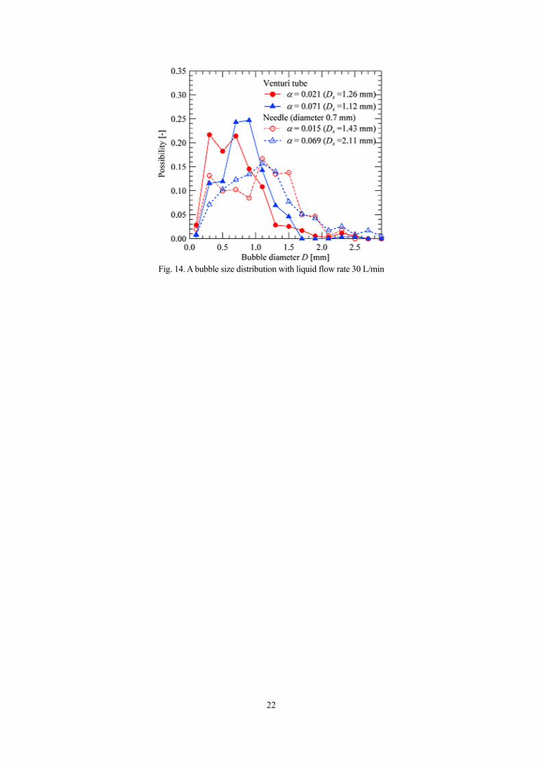
High-speed video camera images between measuring electrodes with the liquid flow rate 30 L/min are shown in Fig. 13. It is confirmed that tiny bubbles with diameters of 100 μm to 1 mm exist in the pipe with the inner diameter of 16 mm. The size distribution of tiny bubbles is shown in Fig. 14. The horizontal axis is bubble diameters and the vertical axis is possibility of tiny bubbles. The solid lines show the size distribution of the bubbles generated with the micro-bubble generator consisted of the venturi tube and the dash lines showed the size distribution of bubbles generated by the needle. SD is Sauter mean diameter. Bubble diameters are measured with counting number of pixels of a vertical length in a snapshot of a bubble which is selected at random. About 300 bubbles are measured. A number of bubbles generated with the venturi tube are confirmed to be micro-bubbles less than 1 mm. Bubbles generated with the venturi tube are miniaturized in comparison with bubbles generated with the needle. From these results, Fig. 12 is the result in dispersed bubbly flow with tiny bubbles with diameters of 100 μm to 1 mm, and then it is proposed that the void fraction measurement by the constant electrical current method is applicable to dispersed bubbly flow with tiny bubbles.

In order to measure the void fraction in dispersed bubbly flow with tiny bubbles, effectiveness of each calculation of the void fraction from the voltage ratio is discussed. The void fraction measured with the constant electrical current method is compared with the void fraction measured with the quick shut valve method. This result is shown in Fig. 15. Benchmarks of voltage ratios and void fractions for the polarization method Eq. (34) v1 and α1 are values when error bars of the void fraction measured with the quick shut valve method are minimums for each liquid flow rates. In Fig. 15, void fractions estimated with each calculation methods are different even if experimental conditions are same as Fig. 10. Especially, overestimates of the void fraction are about 60 % at the maximum for the previous calculation method Eq. (7) in liquid flow rates 20, 25 and 30 L/min. On the other hand, results of Maxwell’s theory Eq. (22) and the polarization method Eq. (34) are coincident with results of the quick shut valve method comparatively. It is made clear that Maxwell’s theory Eq. (22) and the polarization method Eq. (34) are more effective for dispersed bubbly flow with tiny bubbles than the previous method Eq. (7). In comparison with Fig. 10, qualitative difference between the results of Maxwell’s theory Eq. (22) and the polarization method Eq. (34) are not confirmed. However, underestimates of 9 % in Maxwell’s theory Eq. (22) and 20 % in the polarization method Eq. (34) is confirmed in the liquid volume flow ratio 30 L/min.

Results compared between calculation methods of the void fraction and the drift flux model in this experiment are shown in Fig. 16 in order to compare with previous studies. The drift flux model of Eqs. (38), (39) and (40) is applied to disperse bubbly flow with tiny bubbles. Plots show void fractions obtained with each calculation methods based on voltage ratios in Fig. 13. From this result, overestimates of void fractions are about 60 % at the maximum for the previous method Eq. (7). On the other hand, overestimates are 13 % for Maxwell’s theory Eq. (22) and the polarization method. It is confirmed that the void fraction obtained with Maxwell’s theory Eq. (22) and the polarization method Eq. (34) is coincident with drift flux model comparatively. However, the clear difference between the results of Maxwell’s theory Eq. (22) and the polarization method Eq. (34) are not shown as Fig. 15 in comparison with Fig. 11.

Therefore, it is made clear from present study that the constant electrical current method is applicable to dispersed bubbly flow with tiny bubbles with application of Maxwell’s theory Eq. (22) and the polarization method Eq. (34).

4.3. High-speed measurement of void fraction in dispersed bubbly flow

Time series of the void fraction in the liquid volume flow rate 20 L/min is shown in Fig. 17. The horizontal axis is time and the vertical axis is the void fraction estimated with the polarization method Eq. (34). The benchmarks 1α and 1v are the values used in Fig. 10. Plots in this figure show 0.372, 0.169, 0.040 and 0.003 of time-average void fractions. Snapshots in Fig. 18 are observations between measuring electrodes of 0.372 of the time-average void fraction. These observations are coincident with the measurement of the void fraction in Fig. 17.

Temporal fluctuations of time-average void fractions of 0.372 and 0.169 in froth flow have a lot of ups and downs in comparison fluctuations of time-average void fractions with 0.040 and 0.003 in bubbly flow in Fig. 17. From the comparison with the observations in Fig. 18, dispersed bubbles exist between the test section at 0.2643 s of the minimum void fraction in the time-average void fraction 0.372 of Fig. 17. Then, it is confirmed that a large bubble flowed into the test section from 0.2643 s to 0.2917 for rapid increase of the void fraction from 0.2 to 0.67. From 0.2917 s to 0.3165 s, a large bubble passes through the section when the void fraction decreased from 0.67

12

to 0.2 rapidly. Therefore the temporal fluctuation of the void fraction for the flow patterns is confirmed. In addition, gradual temporal fluctuations in time-average void fractions 0.040 and 0.003 in bubbly flow are confirmed. Distributions of the void fraction in flow direction are considered to be inhomogeneous with coalescence of bubbles.

4.4. High-speed measurement of void fraction in dispersed bubbly flow with tiny bubbles

Time series of the void fraction in dispersed bubbly flow with tiny bubbles is shown in Fig. 19. The horizontal axis is time and the vertical axis is the void fraction estimated with the polarization method Eq. (34). The benchmarks 1α and 1v are the values used in Fig. 15. Plots in this figure showed 0.130, 0.077, 0.032 and 0.009 of time-average void fractions. Temporal fluctuations of void fractions in dispersed bubbly flow with tiny bubbles are less than Fig. 17. However, fluctuations are larger with higher void fractions. This cause is considered that distributions of the void fraction in the flow direction are inhomogeneous by coalescence of bubbles. In addition, tiny fluctuations of the void fraction about 0.006 are show in all temporal fluctuations. This is considered electrical noise.

Therefore the constant electric current method with the polarization method is successful in measuring volumetric void fractions with high temporal resolutions. Although this measurement method does not allow to provide two dimensional and three dimensional distributions of void fractions as electric capacitance volume tomography, this method can measure the volumetric void fraction with high spatial resolution of the order of 100 μm and high temporal resolution over 100 kHz in comparison electric capacitance volumetric tomography. Therefore this measurement is expected to provide the volume void fractions in fast flows, shocks and cavitation.

5. Conclusion

In present study, the constant electrical current method is applied to bubbly flow and dispersed bubbly flow with micro-bubbles with diameters of 100 μm to 1 mm. The void fractions in these flows are estimated with Maxwell’s theory and the polarization method. The void fractions estimated with these methods can be more accurate than the previous method. Therefore, this paper proposes that the previous calculation method is applied to annular flow in void fraction 75.0>α [37-39], and Maxwell’s theory and the polarization method are applied to bubbly flow in 30.0<α . In addition, it is also clarified that the Maxwell’s theory and the present proposed method with polarization are compatible with drift flux model, although void fraction estimated with the previous method is higher than the drift flux model for three dimensional dispersed bubbly flow. Furthermore, the constant electric current method with the polarization method is successful in measuring volumetric void fractions with high temporal resolutions. It is experimentally clarified that the present proposed method can follow highly temporal void fluctuation of bubbly and froth flows.

13

References

[1] Kumar SB, Moslemian D, Dudukovi MP. A γ-ray tomographic scanner for imaging voidage distribution in two-phase flow systems,Flow Meas. Instrum., Vol. 6, No. 1, pp. 61-73, 1995. [2] Åbro E, Johansen GA. Improved void fraction determination by means of multibeam gamma-ray attenuation measurements. Flow Measurement and Instrumentation 1999; 10: 99–108. [3] Bruvik EM, Hjertaker BT, Hallanger A. Gamma-ray tomography applied to hydro-carbon multi-phase sampling and slip measurements. Flow Measurement and Instrumentation 2010; 21: 240-248. [4] Asano H, Takenaka N, Fujii T. Flow characteristics of gas–liquid two-phase flow in plate heat exchanger (Visualization and void fraction measurement by neutron radiography). Experimental Thermal and Fluid Science 2004; 28: 223–230. [5] Saito Y, Mishima K, Matsubayashi M, Lim IC, Cha JE, Sim CH. Development of high-resolution high frame-rate neutron radiography. Nuclear Instruments and Method in Physics Research A 2005; 542: 309-315. [6] Hori K, Fujimoto T, Kawanishi K, Nishikawa H. Development of an Ultrafast X-Ray Computed Tomography Scanner System: Application for Measurement of Instantaneous Void Distribution of Gas.Liquid Two-Phase Flow. Heat Transfer—Asian Research 2000; 29 (3):155-165. [7] Fischer F, Hoppe D, Schleicher E, Mattausch G, Flaske H, Bartel R Hampel1 U. An ultra fast electron beam x-ray tomography scanner. Measurement Science and Technology 2008; 19: 094002. [8] Bieberle M, Fischer F, Schleicher E, Franke M, Menz HJ, Mayer HG, Laurien E, Hampel U. Ultrafast Miltiphase Flow Imaging by Electron Beam X-ray Computed Tomography. 7th International Conference on Multiphase Flow ICMF 2010; 2010: 00223. [9] Daidzic NE, Schmidt E, Hasan MM, Altobelli S. Gas–liquid phase distribution and void fraction measurements using MRI. Nuclear Engineering and Design 2005; 235: 1163–1178. [10] Sigrist L, Dossenbach O, Ibl N. On the conductivity and void fraction of gas dispersions in electrolyte solutions. Jornal of Applied Electrochemistry 1980; 10: 223-228. [11] Song CH, Chung MK, No HC. Measurements of void fraction by an improved multi-channel conductance void meter. Nuclear Engineering and Design 1998; 184: 269–285. [12] Fossa M, Guglielmini G, Marchitto A. Intermittent flow parameters from void fraction analysis. Flow Measurement and Instrumentation 2003; 14: 161–168. [13] Kim J, Ahn YC, Kim MH. Measurement of void fraction and bubble speed of slug flow with three-ring conductance probes. Flow Measurement and Instrumentation 2009; 20: 103-109. [14] Schmitz D, Mewes D. Tomographic imaging of transient multiphase flow in bubble columns. Chemical Engineering Journal 2000; 77: 99–104. [15] Prasser HM, Scholz D, Zippe C. Bubble size measurement using wire-mesh sensors. Flow Measurement and Instrumentation 2001; 12: 299–312. [16] Silva MJ, Thiele S, Abdulkareemb L, Azzopardi BJ, Hampel U. High-resolution gas_oil two-phase flow visualization with a capacitance wire-mesh sensor. Flow Measurement and Instrumentation 2010; 21: 191-197. [17] Wang M. Impedance mapping of particulate multiphase flows. Flow Measurement and Instrumentation 2005; 16: 183–189. [18] Jin H, Wang M, Williams RA. Analysis of bubble behaviors in bubble columns using electrical resistance tomography. Chemical Engineering Journal 2007; 130: 179–185. [19] Kendoush AA, Sarkis ZA. Improving the Accuracy of the Capacitance Method for Void Fraction Measurement. Experimental Thermal and Fluid Science 1995; 11: 321-326. [20] Elkow KJ, Rezkallah KS. Void fraction measurements in gas–liquid flows using capacitance sensors. Measurement Science and Technology 1996; 7: 1153–1163.

14

[21] Lowe D, Rezkallah KS. A capacitance sensor for the characterization of microgravity two-phase liquid–gas flows. Measurement Science and Technology 1999; 10: 965–975. [22] Yang HC, Kim DK., Kim MH. Void fraction measurement using impedance method. Flow Measurement and Instrumentation 2003; 14: 151–160. [23] Jaworek A, Krupa A, Trela M. Capacitance sensor for void fraction measurement in water/steam flows. Flow Measurement and Instrumentation 2004; 15: 317–324. [24] Jaworek A, Krupa A. Phase-shift detection for capacitance sensor measuring void fraction in two-phase flow. Sensors and Actuators A 2010; 160: 78–86. [25] Warsito W, Fan LS. Measurement of real-time flow structures in gas–liquid and gas–liquid–solid flow systems using electrical capacitance tomography (ECT). Chemical Engineering Science 2010; 56: 6455–6462. [26] Wang F, Marashdeh Q, Fan LS, Warsito W. Electrical Capacitance Volume Tomography: Design and Applications. Sensors 2010; 10: 1890-1917. [27] Fukano T. Measurement of time varying thickness of liquid film flowing with high speed gas flow by a constant electric current method (CECM). Nuclear Engineering and Design 1998; 184: 363-377. [28] Ide H, Kariyasaki A, Fukano T. Fundamental data on the gas-liquid two-phase flow in minichannels. International Journal of Thermal Sciences. 2007; 46: 519–530. [29] FURUKAWA T, MATSUYAMA F, SADATOMI M. Effects of Reduced Surface Tension on Liquid Film Structure in Vertical Upward Gas-Liquid annular Flows. Journal of power and energy systems 2010; vol.4 no.1. [30] Deendarlianto, Ousaka A, Indarto, Kariyasaki A, Lucas D, Vierow K, Vallee C, Hogan K. The effects of surface tension on flooding in counter-current two-phase flow in an inclined tube. Experimental Thermal and Fluid Science 2010; 34: 813–826. [31] Fujiwara A, Takagi S, Watanabe K, Matsumoto Y. Experimental study on the new micro-bubble gnerator and its appocation to water prification system. Proceedings of FEDSM2003 4th Joint ASME/JSME Fluid Engineering Conference. 2003; FEDSM2003-45162. [32] Minagawa H, Yasuda T, Ishida T. Ultrasonic velocity profile monitor (UVP) measurement of velocity profiles and velocity fluctuation using micro bubbles in turbulent vertical pipe flow. Transactions of the Japan Society of Mechanical Engineers, Series B 2009; 75(750): 41-46. (in Japanese). [33] Maxwell JC. A Treatise on Electricity & Magnetism Vol. NEW YORK: DOVER PUBLICATIONS, INC; 1954 [34] Fujiwara A, Okamoto K, Hashiguchi K, Peixinho j, Takagi S, Matsumoto Y. Bubble breakup phenomena in a venturi tube. Proceedings of FEDSM2007 5th Joint ASME/JSME Fluid Engineering Conference. 2007; FEDSM2007-37243. [35] Ozawa, M. Pressure drop and void fraction. In: The Japan Society of Mechanical Engineers, editors. Handbook of Gas-Liquid Two-Phase Flow Technology Seond Edition. Tokyo: CORONA PUBLISHING CO; 2006, p. 47. (In Japanese). [36] Hibiki T, Ishii M. One-dimensional drift-flux model and constitutive equations for relative motion between phases in various two-phase flow regimes. International Journal of Heat and Mass Transfer 2003; 46: 4935–4948. [37] Xu JL, Cheng P, Zhao TS. Gas-liquid two-phase flow regimes in rectangular channels with mini/micro gaps. International Journal of Multiphase 1999; 25: 411-432. [38] Saisorn S, Wongwise S. A review of two-phase gas-liquid adiabatic flow characteristics in micro-channel. Renewable and Sustainable Energy Reviews 2008; 12: 824-838. [39] Ghajar AJ, Tang CC. Void fraction and flow patterns of two-phase flow in upward and downward vertical and horizaontal pipes. Advances in Multiphase Flow and Heat Transfer. 2010; 4: 231-267.

15

Figure captions Fig. 1. A schematic representation of a vertical upward gas-liquid annular flow (left) and a model of the previous calculation for a annular flow. Fig. 2. Maxwell’s theory: (a) dispersed bubbles within a sphere; (b) a bubble consisted of dispersed bubbles of (a) within a sphere. Fig. 3. A model of the polarization method. Bubbles are assumed to be dielectric bodies. It is assumed that the polarization of atoms or molecules in bubbles cause different electrical field between gas-liquid two-phase flow E′ and liquid single phase flow 0E′ . Fig. 4. A schematic representation of the experimental setup. Fig. 5. A schematic representation of the electrical void fraction meter. Fig. 6. Snapshots of gas injections: (a) with a needle; (b) with a venture tube. Fig. 7. The venturi tube: (a) a snapshot of the venturi tube; (b) a high-speed video camera image of bubble collapses in the diverging region. Fig. 8. The correlation between voltage ratios measured by the constant electric current method and gas-liquid volume flow ratios in bubbly flow and froth flow. Fig. 9. High-speed video camera images of bubbly and froth flow between two measuring electrodes with liquid flow rate 20 L/min Fig. 10. The comparison of void fractions estimated by the constant electric current method and each calculation methods (the previous method Eq. (7), Maxwell’s theory Eq. (22) and the polarization method Eq. (34)) and void fractions measured by the quick shut valve method in bubbly flow and froth flow. Liquid flow rates 20 L/min, 25 L/min and 30 L/min. Fig. 11. The comparison of void fractions estimated by the constant electric current method and each calculation methods (the previous method Eq. (7), Maxwell’s theory Eq. (22) and the polarization method Eq. (34)) and the drift flux models Eqs. (38-40) in bubbly flow and froth flow. Liquid flow rates 20 L/min, 25 L/min and 30 L/min. Fig. 12. The correlation between voltage ratios measured by the constant electric current method and gas-liquid volume flow ratios in bubbly flow with tiny bubbles. Fig. 13. High-speed video camera images of tiny bubbly flow between measuring electrodes with liquid flow rate 30 L/min. Fig. 14. A bubble size distribution with liquid flow rate 30 L/min Fig. 15. The comparison of void fractions estimated by the constant electric current method and each calculation methods (the previous method Eq. (7), Maxwell’s theory Eq. (22) and the polarization method Eq. (34)) and void fractions measured by the quick shut valve method in bubbly flow containing tiny bubbles with diameters of 100 μm – 1 mm. Liquid flow rates 20 L/min, 25 L/min and 30 L/min. Fig. 16. The comparison of void fractions estimated by the constant electric current method and each calculation methods the previous method Eq. (7), Maxwell’s theory Eq. (22) and the polarization method Eq. (34)) and the drift flux models Eqs. (38-40) in bubbly flow containing tiny bubbles with diameters of 100 μm – 1 mm. Liquid flow rates 20 L/min, 25 L/min and 30 L/min. Fig. 17. Temporal fluctuations of void fractions in bubbly flow and froth flow with liquid flow rate 20 L/min Fig. 18. High-speed video camera images between measuring electrodes with the time-average void fraction 0.372 and the liquid flow rate 20 L/min. Fig. 19. Temporal fluctuations of void fractions in bubbly flow containing tiny bubbles with diameters of 100 mm – 1mm. Liquid flow rate is 30 L/min.

16

Fig. 1. A schematic representation of a vertical upward gas-liquid annular flow (left) and a model of the previous calculation for a annular flow.

Fig. 2. Maxwell’s theory: (a) dispersed bubbles within a sphere; (b) a bubble consisted of dispersed bubbles of (a) within a

sphere.

17

Fig. 3. A model of the polarization method. Bubbles are assumed to be dielectric bodies. It is assumed that the polarization of atoms or molecules in bubbles cause different electrical field between gas-liquid two-phase flow E′ and liquid single phase flow 0E′ .

Fig. 4. A schematic representation of the experimental setup.

Fig. 5. A schematic representation of the electrical void fraction meter.

18

Fig. 5. A schematic representation of the electrical void fraction meter.

Fig. 6. Snapshots of gas injections: (a) with a needle; (b) with a venture tube.

Fig. 7. The venturi tube: (a) a snapshot of the venturi tube; (b) a high-speed video camera image of bubble collapses in the diverging region.

19

Fig. 8. The correlation between voltage ratios measured by the constant electric current method and gas-liquid volume flow ratios in bubbly flow and froth flow.

Fig. 9. High-speed video camera images of bubbly and froth flow between two measuring electrodes with liquid flow rate 20 L/min

20

Fig. 10. The comparison of void fractions estimated by the constant electric current method and each calculation methods (the previous method, Maxwell’s theory and the polarization method) and void fractions measured by the quick shut valve method in bubbly flow and froth flow. Liquid flow rates 20 L/min, 25 L/min and 30 L/min. Fig. 11. The comparison of void fractions estimated by the constant electric current method and each calculation methods (the previous method, Maxwell’s theory and the polarization method) and the drift flux models Eqs. (38-40) in bubbly flow and froth flow. Liquid flow rates 20 L/min, 25 L/min and 30 L/min.

21

Fig. 12. The correlation between voltage ratios measured by the constant electric current method and gas-liquid volume flow ratios in bubbly flow with tiny bubbles.

Fig. 13. High-speed video camera images of tiny bubbly flow between measuring electrodes with liquid flow rate 30 L/min.

22

Fig. 14. A bubble size distribution with liquid flow rate 30 L/min

23

Fig. 15. The comparison of void fractions estimated by the constant electric current method and each calculation methods (the previous method, Maxwell’s theory and the polarization method) and void fractions measured by the quick shut valve method in bubbly flow containing tiny bubbles with diameters of 100 μm – 1 mm. Liquid flow rates 20 L/min, 25 L/min and 30 L/min. Fig. 16. The comparison of void fractions estimated by the constant electric current method and each calculation methods (the previous method, Maxwell’s theory and the polarization method) and the drift flux models Eqs. (38-40) in bubbly flow containing tiny bubbles with diameters of 100 μm – 1 mm. Liquid flow rates 20 L/min, 25 L/min and 30 L/min.

24

Fig. 17. Temporal fluctuations of void fractions in bubbly flow and froth flow with liquid flow rate 20 L/min

Fig. 18. High-speed video camera images between measuring electrodes with the time-average void fraction 0.372 and the liquid flow rate 20 L/min.

25

Fig. 19. Temporal fluctuations of void fractions in bubbly flow containing tiny bubbles with diameters of 100 mm – 1mm. Liquid flow rate is 30 L/min.