measurement and modeling of energetic- material mass
TRANSCRIPT
SANDIA REPORT SAND2006-2611 Unlimited Release Printed May 2006
Measurement and Modeling of Energetic-Material Mass Transfer to Soil-Pore Water – Project CP-1227 Final Technical Report Stephen W. Webb, James M. Phelan, Teklu Hadgu, Joshua S. Stein, and Cedric M. Sallaberry Prepared by Sandia National Laboratories Albuquerque, New Mexico 87185 and Livermore, California 94550 Sandia is a multiprogram laboratory operated by Sandia Corporation, a Lockheed Martin Company, for the United States Department of Energy’s National Nuclear Security Administration under Contract DE-AC04-94AL85000. Approved for public release; further dissemination unlimited.
2
Issued by Sandia National Laboratories, operated for the United States Department of Energy by Sandia Corporation. NOTICE: This report was prepared as an account of work sponsored by an agency of the United States Government. Neither the United States Government, nor any agency thereof, nor any of their employees, nor any of their contractors, subcontractors, or their employees, make any warranty, express or implied, or assume any legal liability or responsibility for the accuracy, completeness, or usefulness of any information, apparatus, product, or process disclosed, or represent that its use would not infringe privately owned rights. Reference herein to any specific commercial product, process, or service by trade name, trademark, manufacturer, or otherwise, does not necessarily constitute or imply its endorsement, recommendation, or favoring by the United States Government, any agency thereof, or any of their contractors or subcontractors. The views and opinions expressed herein do not necessarily state or reflect those of the United States Government, any agency thereof, or any of their contractors. Printed in the United States of America. This report has been reproduced directly from the best available copy. Available to DOE and DOE contractors from U.S. Department of Energy Office of Scientific and Technical Information P.O. Box 62 Oak Ridge, TN 37831 Telephone: (865) 576-8401 Facsimile: (865) 576-5728 E-Mail: [email protected] Online ordering: http://www.osti.gov/bridge Available to the public from U.S. Department of Commerce National Technical Information Service 5285 Port Royal Rd. Springfield, VA 22161 Telephone: (800) 553-6847 Facsimile: (703) 605-6900 E-Mail: [email protected] Online order: http://www.ntis.gov/help/ordermethods.asp?loc=7-4-0#online
3
SAND2006-2611 Unlimited Release Printed May 2006
Measurement and Modeling of Energetic-Material Mass Transfer to Soil-Pore Water – Project CP-1227
Final Technical Report
Stephen W. Webb Geohydrology Department
James M. Phelan
Contraband Detection Department
Teklu Hadgu, Joshua S. Stein, and Cedric M. Sallaberry Subsystems Performance Assessment Department
Sandia National Laboratories
P.O. Box 5800 Albuquerque, NM 87185-0735
Abstract Military test and training ranges operate with live-fire engagements to provide realism important to the maintenance of key tactical skills. Ordnance detonations during these operations typically produce minute residues of parent explosive chemical compounds. Occasional low-order detonations also disperse solid-phase energetic material onto the surface soil. These detonation remnants are implicated in chemical contamination impacts to groundwater on a limited set of ranges where environmental characterization projects have occurred. Key questions arise regarding how these residues and the environmental conditions (e.g., weather and geostratigraphy) contribute to groundwater pollution. This final report documents the results of experimental and simulation model development for evaluating mass-transfer processes from solid-phase energetics to soil-pore water.

4
Acknowledgements This work was sponsored by the Strategic Environmental Research and Development Program (SERDP) under the technical direction of Jeff Marqusee and programmatic direction of Brad Smith and Andrea Leeson. The authors thank James Barnett, Dayle Kerr, Joseph Romero, and Fawn Griffin for their extensive support for the laboratory testing and Mehdi Eliassi for contributions to the model development work; without their support, none of this work could have been achieved.
5
Contents
1. Introduction............................................................................................................................13 1.1 Purpose............................................................................................................................13 1.2 Work Task Schedule .......................................................................................................13
2. Background ............................................................................................................................17 2.1 Energetic Material Deposits............................................................................................17 2.2 Solid-Phase Energetic Materials in Soils........................................................................18 2.3 Importance of Surface Conditions ..................................................................................19 2.4 Mass Transfer from Energetic Materials to Water .........................................................20
3. Project Plan ............................................................................................................................23 3.1 Task 1: Experimental .....................................................................................................23 3.2 Task 2: Modeling ...........................................................................................................25
4. Experimental Methods ..........................................................................................................27 4.1 Test Plans ........................................................................................................................27 4.2 Chemical Analysis ..........................................................................................................27
4.2.1 High-Pressure Liquid Chromatography (HPLC) Method .................................27 4.3 Energetic Material...........................................................................................................28
4.3.1 Comp B Source Material ...................................................................................28 4.3.2 Low-Order Detonation Debris...........................................................................31
4.4 Dissolution Kinetics........................................................................................................33 4.5 Porous Media Characterization.......................................................................................33
4.5.1 Physical/Hydraulic Properties ...........................................................................33 4.5.2 Aqueous-Solid Partitioning ...............................................................................38
4.6 Saturated Flow Test Methods .........................................................................................38 4.7 Unsaturated Flow Test Methods .....................................................................................40
4.7.1 Rain Simulator...................................................................................................42 4.8 Degradation.....................................................................................................................42
4.8.1 Slurry Tests with Aqueous Samples..................................................................43 4.8.2 Slurry Sacrifice Tests ........................................................................................45
5. Experimental Results.............................................................................................................47 5.1 Data Analysis Methods...................................................................................................47 5.2 Phase I Test Results ........................................................................................................53
5.2.1 Scoping Test 1 ...................................................................................................53 5.2.2 Scoping Test 2 ...................................................................................................55 5.2.3 Test 3: Effect of Flow and Temperature ..........................................................57
5.3 Phase II Test Results.......................................................................................................59 5.3.1 Effect of Bed Loading .......................................................................................59 5.3.2 Effect of Bed Depth...........................................................................................61 5.3.3 Effect of Initial Mass.........................................................................................64 5.3.4 Effect of Flow....................................................................................................66 5.3.5 Effect of Temperature .......................................................................................69 5.3.6 Effect Of Energetic Material Particle Size ........................................................71
6
5.3.7 Effect of Initial Wetting Phase ..........................................................................73 5.3.8 Effect of Porous Media Saturation ....................................................................75 5.3.9 Effect Of Pulsed Water Flow ............................................................................79 5.3.10 Effect of Low-Order Detonation Debris I .........................................................83
5.4 Phase III Test Results .....................................................................................................84 5.4.1 Effect of Test Replication..................................................................................85 5.4.2 Effect of Bed Location ......................................................................................87 5.4.3 Effect of Energetic Material Particle Size.........................................................89 5.4.4 Effect of Low-Order Detonation Debris II........................................................92
5.5 Mass Balance ..................................................................................................................95 6. Model Development ...............................................................................................................97
6.1 Mass Transfer Formulation.............................................................................................97 6.2 Simulation Model ...........................................................................................................98 6.3 Simulation Parameters ..................................................................................................100
6.3.1 Parameter Definitions......................................................................................100 6.3.2 Assigned Values for Simulation Parameters ...................................................101
7. Data Model Comparisons....................................................................................................103 7.1 Illustrative Simulation Results of Column Experiments ..............................................103 7.2 Results for Individual Tests ..........................................................................................106
7.2.1 Saturated Flow Tests .......................................................................................107 7.2.2 Pulse Tests.......................................................................................................116
7.3 Mass Transfer Parameters.............................................................................................118 7.4 Discussion.....................................................................................................................121
8. Summary...............................................................................................................................123 8.1 Experimental Results ....................................................................................................123
8.1.1 Phases I and II .................................................................................................123 8.1.2 Phase III...........................................................................................................124
8.2 Modeling.......................................................................................................................125 9. Conclusions...........................................................................................................................127 Appendix A—Zero Dimensional Mass Transfer Model.........................................................133 Appendix B—Mass Transfer Parameter Regression Analysis..............................................143
7
Figures Figure 1. Low-Order Detonation Debris Containing TNT Main Charge (~30 cm long) .............17 Figure 2. Soil Aggregate Containing Soot and Extractable TNT (~5 cm long axis)....................17 Figure 3. Unreacted TNT Ejected from Low Order Detonation (~5 cm dia) ...............................18 Figure 4. Effect of Soil Water Partitioning Coefficient (Kd) on Maximum Soil Residue for
RDX.........................................................................................................................19 Figure 5. Laboratory Experimental Apparatus .............................................................................24 Figure 6. Simulation Modeling Approach ....................................................................................25 Figure 7. Comp B Starting Material .............................................................................................29 Figure 8. SEM Photograph of 500- to 600-μm size fraction ........................................................30 Figure 9. Glass Bead Particle Size Distribution ...........................................................................34 Figure 10. Primary Drainage Results for Glass Bead Tension versus Saturation ........................35 Figure 11. Glass-Bead Moisture Characteristic Curve (Table 10) ...............................................37 Figure 12. Unsaturated Hydraulic Conductivity Prediction Using Mualem, Eq. [7] ...................37 Figure 13. Saturated Column Schematic ......................................................................................40 Figure 14. Flow Cell and Effluent Color ......................................................................................40 Figure 15. Unsaturated Flow Apparatus .......................................................................................41 Figure 16. Unsaturated Flow Column, Comp B layer, Tensiometers...........................................41 Figure 17. Tensiometer Assembly ................................................................................................41 Figure 18. Slurry Test 1X Results ................................................................................................44 Figure 19. Slurry Test 5X Results ................................................................................................45 Figure 20. Slurry Sacrifice Test Results – Zero-Order Degradation Plot.....................................46 Figure 21. Slurry Sacrifice Test Results – First-Order Degradation Plot.....................................46 Figure 22. Compiled RDX and TNT Solubility Data ...................................................................47 Figure 23. Early Time Dissolution Results...................................................................................49 Figure 24. Full Duration Dissolution Results ...............................................................................49 Figure 25. Derived Dissolution Flux for Comp B Particles in Water...........................................52 Figure 26. Test 1: Concentration and Flux Density......................................................................54 Figure 27. Test 2: Concentration, Temperature, and Flux Density ..............................................55 Figure 28. Test 2: TNT and RDX C/Cmax ....................................................................................55 Figure 29. Test 2: Cumulative Discharge .....................................................................................56 Figure 30. Test 3: Concentration, Temperature, and Flux Density ..............................................57 Figure 31. Test 3: TNT and RDX C/Cmax. ....................................................................................58 Figure 32. Test 3: Cumulative Discharge ....................................................................................58 Figure 33. Effect of Bed Loading – Effluent Concentration (C/Cmax), RDX ...............................60 Figure 34. Effect of Bed Loading – Effluent Concentration (C/Cmax), TNT ................................60 Figure 35. Effect of Bed Loading – Cumulative Discharge, RDX...............................................61 Figure 36. Effect of Bed Loading – Cumulative Discharge, TNT................................................61 Figure 37. Effect of Bed Depth - Effluent Concentration (C/Cmax), RDX....................................62 Figure 38. Effect of Bed Depth - Effluent Concentration (C/Cmax), TNT ....................................63 Figure 39. Effect of Bed Depth – Cumulative Discharge, RDX ..................................................63 Figure 40. Effect of Bed Depth – Cumulative Discharge, TNT ...................................................64 Figure 41. Effect of Initial Mass – Effluent Concentration (C/Cmax), RDX .................................65 Figure 42. Effect of Initial Mass – Effluent Concentration (C/Cmax), TNT..................................65
8
Figure 43. Effect of Initial Mass – Cumulative Discharge, RDX.................................................66 Figure 44. Effect of Initial Mass – Cumulative Discharge, TNT .................................................66 Figure 45. Effect of Flow – Effluent Concentration, RDX...........................................................67 Figure 46. Effect of Flow – Effluent Concentration, TNT ...........................................................68 Figure 47. Effect of Flow – Cumulative Discharge, RDX ...........................................................68 Figure 48. Effect of Flow – Cumulative Discharge, TNT ............................................................69 Figure 49. Effect of Temperature – Effluent Concentration, RDX ..............................................69 Figure 50. Effect of Temperature – Effluent Concentration, RDX C/Cmax ..................................70 Figure 51. Effect of Temperature – Effluent Concentration, TNT...............................................70 Figure 52. Effect of Temperature – Effluent Concentration, RDX C/Cmax ..................................71 Figure 53. Effect of Energetic Material Particle Size – RDX C/Cmax...........................................72 Figure 54. Effect of Energetic Material Particle Size – TNT C/Cmax ...........................................73 Figure 55. Effect of Initial Wetting Rate – Effluent Concentration, RDX...................................74 Figure 56. Effect of Initial Wetting Rate – Effluent Concentration, TNT....................................74 Figure 57. Effect of Initial Wetting Rate – Cumulative Discharge, RDX....................................75 Figure 58. Effect of Initial Wetting Rate – Cumulative Discharge, TNT ....................................75 Figure 59. Column Wetting Phase – Matric Potential with Tensiometers ...................................76 Figure 60. Column Saturation and Effluent Flux During Unsaturated Flow Test MT5...............77 Figure 61. Effect of Porous Media Saturation – Effluent Concentration, RDX...........................78 Figure 62. Effect of Porous Media Saturation – Effluent Concentration, TNT............................78 Figure 63. Column Matric Potential (Tensiometer 1) During Pulse Test MT5............................80 Figure 64. Column Matric Potential (Tensiometer 1) During Pulse Test MT12..........................81 Figure 65. Effect of Pulsed Water Flow – Effluent Concentration (C/Cmax), RDX and TNT......82 Figure 66. Glass Bead Moisture Content Check Samples ............................................................82 Figure 67. Effect of Low-Order Detonation Debris – Effluent Concentration C/Cmax, RDX ......84 Figure 68. Effect of Low-Order Detonation Debris – Effluent Concentration (C/Cmax), TNT ....84 Figure 69. Effect of Test Replication – Effluent Concentration (C/Cmax), RDX..........................85 Figure 70. Effect of Test Replication – Effluent Concentration (C/Cmax), TNT ..........................86 Figure 71. Effect of Test Replication – Cumulative Discharge, RDX .........................................86 Figure 72. Effect of Test Replication – Cumulative Discharge, TNT..........................................87 Figure 73. Effect of Bed Location – Effluent Concentration (C/Cmax), RDX...............................88 Figure 74. Effect of Bed Location – Effluent Concentration (C/Cmax), TNT ...............................88 Figure 75. Effect of Bed Location – Cumulative Discharge, RDX..............................................89 Figure 76. Effect of Bed Location – Cumulative Discharge, TNT...............................................89 Figure 77. Effect of Energetic Material Particle Size - Effluent Concentration (C/Cmax), RDX..90 Figure 78. Effect of Energetic Material Particle Size – Effluent Concentration (C/Cmax), TNT..91 Figure 79. Effect of Energetic Material Particle Size – Cumulative Discharge, RDX.................91 Figure 80. Effect of Energetic Material Particle Size – Cumulative Discharge, TNT .................92 Figure 81. Effect of Low-Order Detonation Debris – Effluent Concentration (C/Cmax), RDX....93 Figure 82. Effect of Low-Order Detonation Debris – Effluent Concentration (C/Cmax), TNT ....93 Figure 83. Effect of Low-Order Detonation Debris – Cumulative Discharge, TNT....................95 Figure 84. Simulation Models for Saturated Flow Experiments ..................................................99 Figure 85. Simulation Models for Unsaturated Flow Experiments ..............................................99 Figure 86. Experimental Stages ..................................................................................................104 Figure 87. Effect of Surface Area Exponent X on Model Response for MT7 ...........................104 Figure 88. Effect of Mass Transfer Coefficient k on Model Response for MT7 .......................105
9
Figure 89. Effect of Solid Sorption Coefficient Kd on Model Response for MT7 .....................105 Figure 90. Data-Model Comparison for MT6 ............................................................................107 Figure 91. Data-Model Comparison for MT7 ............................................................................107 Figure 92. Data-Model Comparison for MT8 ............................................................................108 Figure 93. Data-Model Comparison for MT9b2 ........................................................................109 Figure 94. Data-Model Comparison for MT9b3 ........................................................................109 Figure 95. Data-Model Comparison for MT10 ..........................................................................110 Figure 96. Data-Model Comparison for MT13 ..........................................................................110 Figure 97. Data-Model Comparison for MT14. .........................................................................111 Figure 98. Data-Model Comparison for MT12 for Exit RDX Concentration ............................117 Figure 99. Data-Model Comparison for MT12 for Outflow Volumetric Water Flux ................117 Figure 100. Data-Model Comparison for MT12 for Cumulative RDX Mass ............................118 Figure 101. Effect of Initial Particle Diameter on Mass Transfer Coefficient, k .......................120 Figure 102. Effect of Initial Particle Diameter on Interfacial Area Exponent, X .......................120 Figure 103. Peak Concentrations of RDX and TNT in the Saturated Flow Tests ......................123 Figure 104. Science and Technology Roadmap .........................................................................127 Figure 105. Two-dimensional conceptual embodiment of the Screening Toolset model ..........128
10
Tables Table 1. Project Task Schedule.....................................................................................................13 Table 2. Master List of Tasks, Milestones and Deliverables........................................................15 Table 3. Experimental Test Phases and Principal Factors ............................................................27 Table 4. RDX and TNT Standard Compositions ..........................................................................28 Table 5. Calibration Chart for RDX and TNT Standards .............................................................28 Table 6. Sieve Series.....................................................................................................................29 Table 7. RDX and TNT Mass Fraction in Each Size Separate.....................................................30 Table 8. Specific Surface Area of Comp B Size Separates ..........................................................30 Table 9. Detonation Debris Analytical Results – Discrete Samples (μg/g)..................................31 Table 10. Low-Order Detonation Debris, 81-mm Mortar, Blossom Point, May 2002 ................31 Table 11. BET Specific Surface Area Measurements, Low-Order Detonation Debris, 81-
mm Mortar, Blossom Point, May 2002...................................................................32 Table 12. RDX, TNT and Comp B Content of Bag 6 and Bag 8, Low-Order Detonation
Debris ......................................................................................................................33 Table 13. Moisture Characteristic Curve Values from RETC Program.......................................36 Table 14. Soda-Lime, Glass-Bead, Aqueous-Solid Partitioning Data and Results ......................38 Table 15. Specifications of Saturated Columns............................................................................39 Table 16. Aqueous Solubility Empirical Correlation ...................................................................47 Table 17. Average Dissolution Flux (ng/cm2-sec) for Each Particle Size....................................52 Table 18. Summary Table – Saturated Flow Test Variables ........................................................53 Table 19. Test Parameters – Effect of Bed Loading.....................................................................59 Table 20. Test Parameters – Effect of Bed Depth ........................................................................62 Table 21. Effect of Initial Mass ....................................................................................................64 Table 22. Test Parameters – Effect of Flow .................................................................................67 Table 23. Test Parameters – Effect of Energetic Material Particle Size.......................................72 Table 24. Test Parameters – Effect of Initial Wetting Phase........................................................73 Table 25. Unsaturated Flow Test MT5 Saturation and Flow Schedule........................................76 Table 26. Saturation, Matric Potential, and Equivalent Pore Radius ...........................................79 Table 27. Pulsed Test Water Inflow .............................................................................................80 Table 28. Detonation Debris Analytical Results – Combined Sample.........................................83 Table 29. Effect of Low-Order Detonation Debris.......................................................................83 Table 30. Test Parameters – Effect of Test Replication ...............................................................85 Table 31. Test Parameters – Effect of Bed Location ....................................................................87 Table 32. Test Parameters – Effect of Energetic Material Particle Size.......................................90 Table 33. Test Parameters – Effect of Low-Order Detonation Debris .........................................92 Table 34. Heterogeneity of Low-Order Detonation Debris ..........................................................94 Table 35. Effect of Low-Order Detonation Debris – Cumulative Discharge, RDX.....................94 Table 36. Mass Balance of RDX and TNT (Phase I) ...................................................................95 Table 37. Mass Balance of RDX (Phase III) ................................................................................96 Table 38. Mass Balance of TNT (Phase III) .................................................................................96 Table 39. Phase I Experiment Duration (hours) ...........................................................................96 Table 40. Simulation Parameters ................................................................................................101 Table 41. Mass Transfer Parameters...........................................................................................119

11
Acronyms BET Brunauer, Emmett, and Teller DNB dinitrobenzene DNT dinitrotoluene GC/ECD Gas chromatography/electron capture detector HPLC high-pressure liquid chromatography IPR internal program review mL milliliter NAPL nonaqueous phase liquid R&D research and development RDX research department explosive RETC retention curve RP-HPLC Reverse-Phase High-Pressure Liquid Chromatography S&T science and technology SEM scanning electron microscopy SERDP Strategic Environmental Research and Development Program SON Statement of Need TNT trinitrotoluene UXO unexploded ordnance

12
13
1. Introduction The Strategic Environmental Research and Development Program (SERDP) seeks techniques and knowledge that will permit assessment of the environmental impact of residual energetic material from test and training operations. Low-order detonations that disperse discrete solid-phase particles onto and into the soil leave the greatest legacy of energetic material residues. One principal environmental impact is the contamination of aquifers. The energetic material most likely to impact aquifers is research department explosive (RDX) due to its low drinking water advisory limits, low retardation during soil transport, and low rate of environmental degradation. Understanding the mass transfer rate from discrete, solid-phase particles into the soil-pore water is critical to the impact analysis of these residues for groundwater contamination. Weather is an important process that drives the mass-transfer phenomena. This work analyzes this mass-transfer process using laboratory measurement and numerical simulation methods. The results from this work provide the foundation for a new predictive ability to assess the migration potential of residual energetic materials. 1.1 Purpose
The purpose of this work was to develop an energetic material source release function that describes the mass transfer of solid-phase energetic materials to a solute in soil-pore water that could be used in a solute transport model with linkages to time-dependent weather phenomena. This source-release function is based on experimental data obtained during this investigation. 1.2 Work Task Schedule
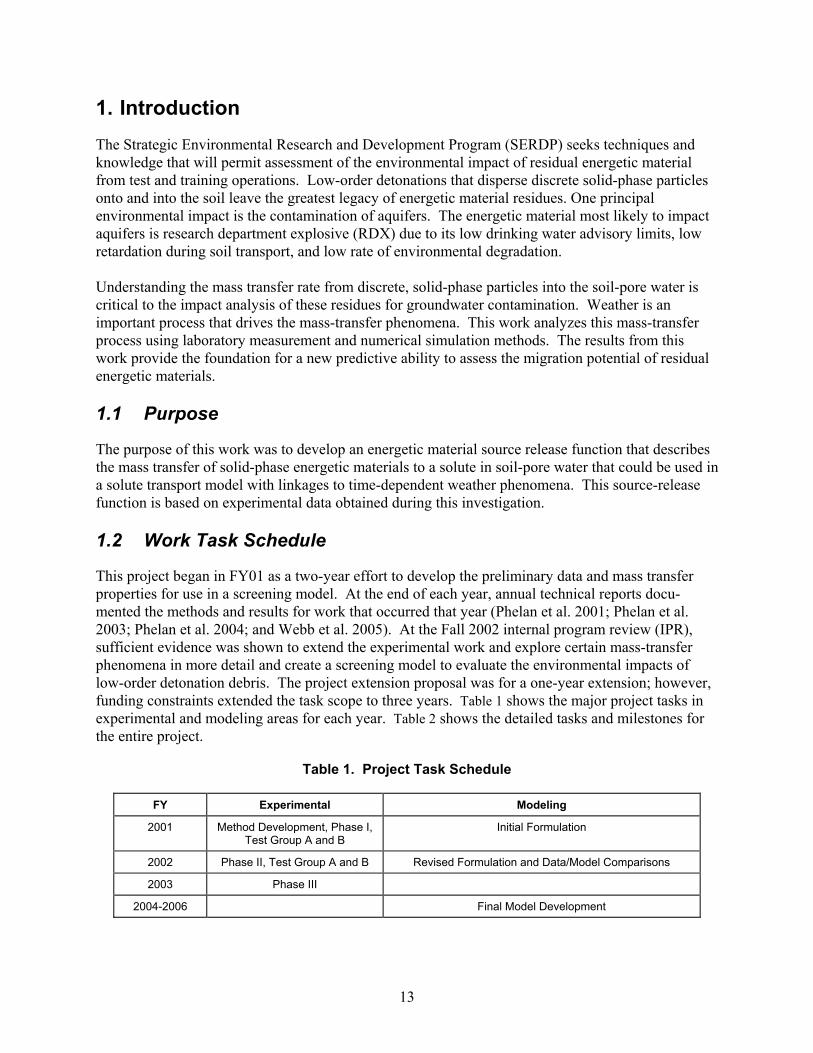
This project began in FY01 as a two-year effort to develop the preliminary data and mass transfer properties for use in a screening model. At the end of each year, annual technical reports docu-mented the methods and results for work that occurred that year (Phelan et al. 2001; Phelan et al. 2003; Phelan et al. 2004; and Webb et al. 2005). At the Fall 2002 internal program review (IPR), sufficient evidence was shown to extend the experimental work and explore certain mass-transfer phenomena in more detail and create a screening model to evaluate the environmental impacts of low-order detonation debris. The project extension proposal was for a one-year extension; however, funding constraints extended the task scope to three years. Table 1 shows the major project tasks in experimental and modeling areas for each year. Table 2 shows the detailed tasks and milestones for the entire project.
Table 1. Project Task Schedule
FY Experimental Modeling
2001 Method Development, Phase I, Test Group A and B
Initial Formulation
2002 Phase II, Test Group A and B Revised Formulation and Data/Model Comparisons
2003 Phase III
2004-2006 Final Model Development

14
The experimental data were obtained between 2001 and 2003. The initial Energetic Material Source Function was formulated in 2001 and compared to experimental data in 2002. The final Energetic Material Source Function was developed in 2005 as detailed in this report. This report also serves as the final project report. This report is a compilation of the technical report deliverables published on this project as listed in Table 2. This compilation was made to provide all the information generated in a single document. The only exceptions are that the initial model development presented in Phelan et al. (2003) has not been included because it has been superseded by more recent efforts as presented in Section 7.0, and SAND2002-2420 (Phelan et al., 2002) is not included.
15
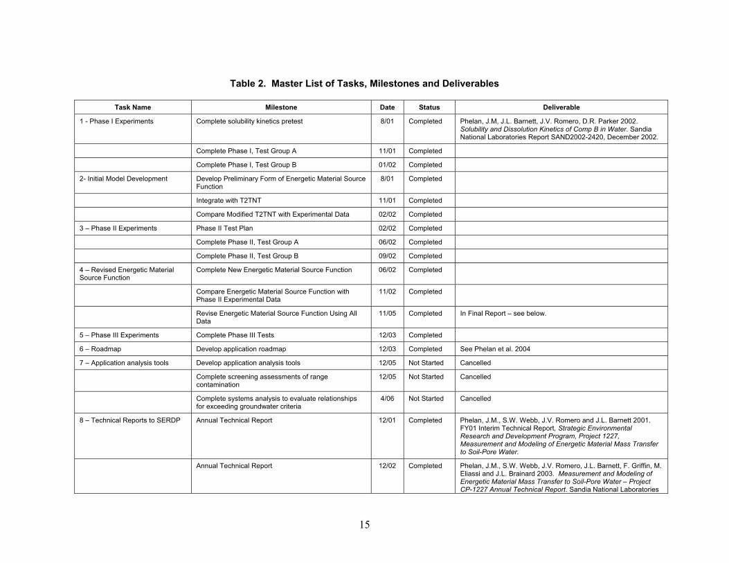
Table 2. Master List of Tasks, Milestones and Deliverables
Task Name Milestone Date Status Deliverable
1 - Phase I Experiments Complete solubility kinetics pretest 8/01 Completed Phelan, J.M, J.L. Barnett, J.V. Romero, D.R. Parker 2002. Solubility and Dissolution Kinetics of Comp B in Water. Sandia National Laboratories Report SAND2002-2420, December 2002.
Complete Phase I, Test Group A 11/01 Completed
Complete Phase I, Test Group B 01/02 Completed
2- Initial Model Development Develop Preliminary Form of Energetic Material Source Function
8/01 Completed
Integrate with T2TNT 11/01 Completed
Compare Modified T2TNT with Experimental Data 02/02 Completed
3 – Phase II Experiments Phase II Test Plan 02/02 Completed
Complete Phase II, Test Group A 06/02 Completed
Complete Phase II, Test Group B 09/02 Completed
4 – Revised Energetic Material Source Function
Complete New Energetic Material Source Function 06/02 Completed
Compare Energetic Material Source Function with Phase II Experimental Data
11/02 Completed
Revise Energetic Material Source Function Using All Data
11/05 Completed In Final Report – see below.
5 – Phase III Experiments Complete Phase III Tests 12/03 Completed
6 – Roadmap Develop application roadmap 12/03 Completed See Phelan et al. 2004
7 – Application analysis tools Develop application analysis tools 12/05 Not Started Cancelled
Complete screening assessments of range contamination
12/05 Not Started Cancelled
Complete systems analysis to evaluate relationships for exceeding groundwater criteria
4/06 Not Started Cancelled
8 – Technical Reports to SERDP Annual Technical Report 12/01 Completed Phelan, J.M., S.W. Webb, J.V. Romero and J.L. Barnett 2001. FY01 Interim Technical Report, Strategic Environmental Research and Development Program, Project 1227, Measurement and Modeling of Energetic Material Mass Transfer to Soil-Pore Water.
Annual Technical Report 12/02 Completed Phelan, J.M., S.W. Webb, J.V. Romero, J.L. Barnett, F. Griffin, M. Eliassi and J.L. Brainard 2003. Measurement and Modeling of Energetic Material Mass Transfer to Soil-Pore Water – Project CP-1227 Annual Technical Report. Sandia National Laboratories
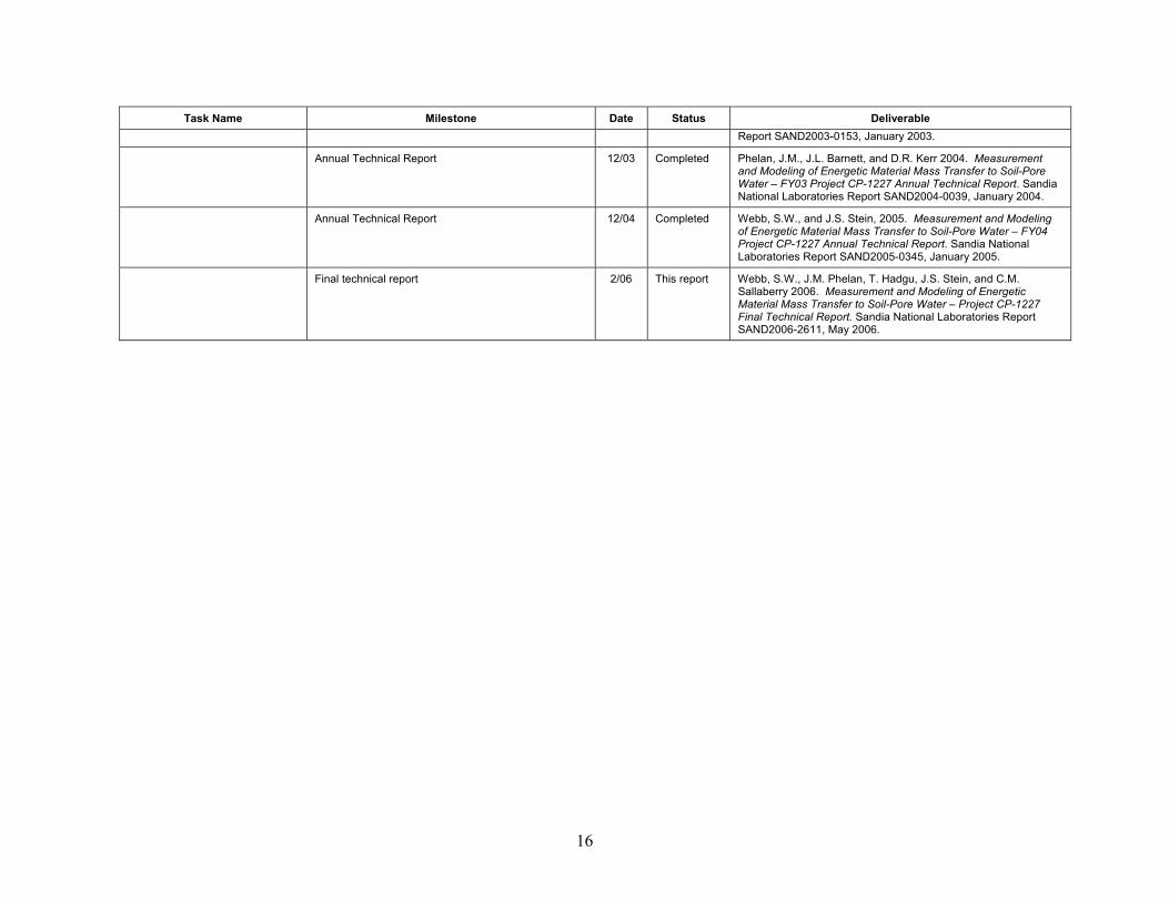
16
Task Name Milestone Date Status Deliverable Report SAND2003-0153, January 2003.
Annual Technical Report 12/03 Completed Phelan, J.M., J.L. Barnett, and D.R. Kerr 2004. Measurement and Modeling of Energetic Material Mass Transfer to Soil-Pore Water – FY03 Project CP-1227 Annual Technical Report. Sandia National Laboratories Report SAND2004-0039, January 2004.
Annual Technical Report 12/04 Completed Webb, S.W., and J.S. Stein, 2005. Measurement and Modeling of Energetic Material Mass Transfer to Soil-Pore Water – FY04 Project CP-1227 Annual Technical Report. Sandia National Laboratories Report SAND2005-0345, January 2005.
Final technical report 2/06 This report Webb, S.W., J.M. Phelan, T. Hadgu, J.S. Stein, and C.M. Sallaberry 2006. Measurement and Modeling of Energetic Material Mass Transfer to Soil-Pore Water – Project CP-1227 Final Technical Report. Sandia National Laboratories Report SAND2006-2611, May 2006.
17
2. Background
2.1 Energetic Material Deposits
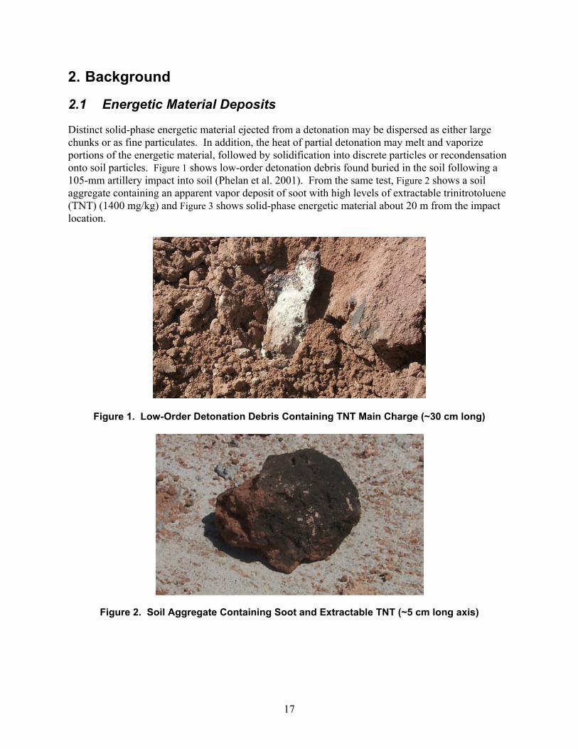
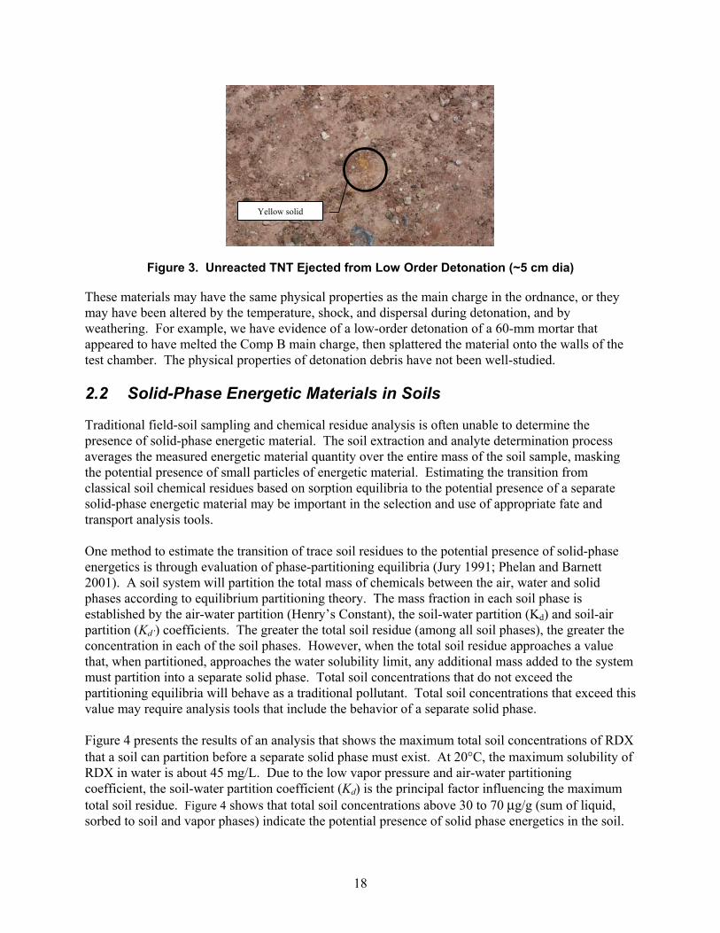
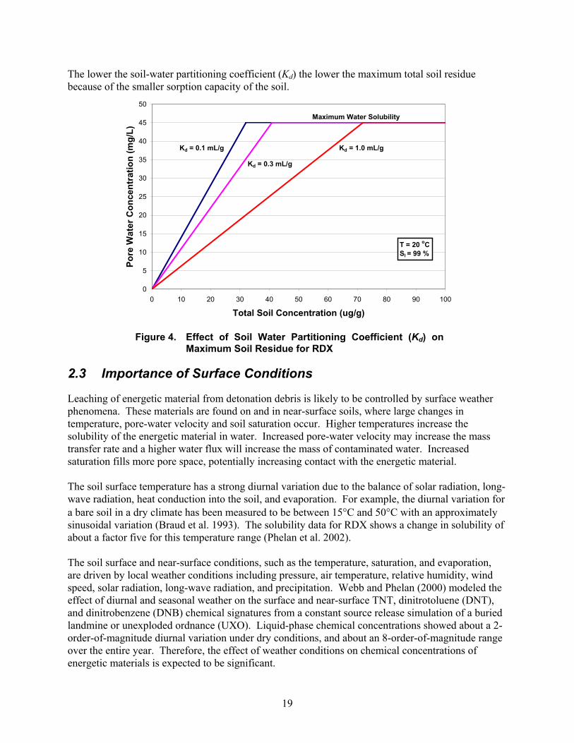
Distinct solid-phase energetic material ejected from a detonation may be dispersed as either large chunks or as fine particulates. In addition, the heat of partial detonation may melt and vaporize portions of the energetic material, followed by solidification into discrete particles or recondensation onto soil particles. Figure 1 shows low-order detonation debris found buried in the soil following a 105-mm artillery impact into soil (Phelan et al. 2001). From the same test, Figure 2 shows a soil aggregate containing an apparent vapor deposit of soot with high levels of extractable trinitrotoluene (TNT) (1400 mg/kg) and Figure 3 shows solid-phase energetic material about 20 m from the impact location.
Figure 1. Low-Order Detonation Debris Containing TNT Main Charge (~30 cm long)
Figure 2. Soil Aggregate Containing Soot and Extractable TNT (~5 cm long axis)
18
Figure 3. Unreacted TNT Ejected from Low Order Detonation (~5 cm dia)
These materials may have the same physical properties as the main charge in the ordnance, or they may have been altered by the temperature, shock, and dispersal during detonation, and by weathering. For example, we have evidence of a low-order detonation of a 60-mm mortar that appeared to have melted the Comp B main charge, then splattered the material onto the walls of the test chamber. The physical properties of detonation debris have not been well-studied. 2.2 Solid-Phase Energetic Materials in Soils
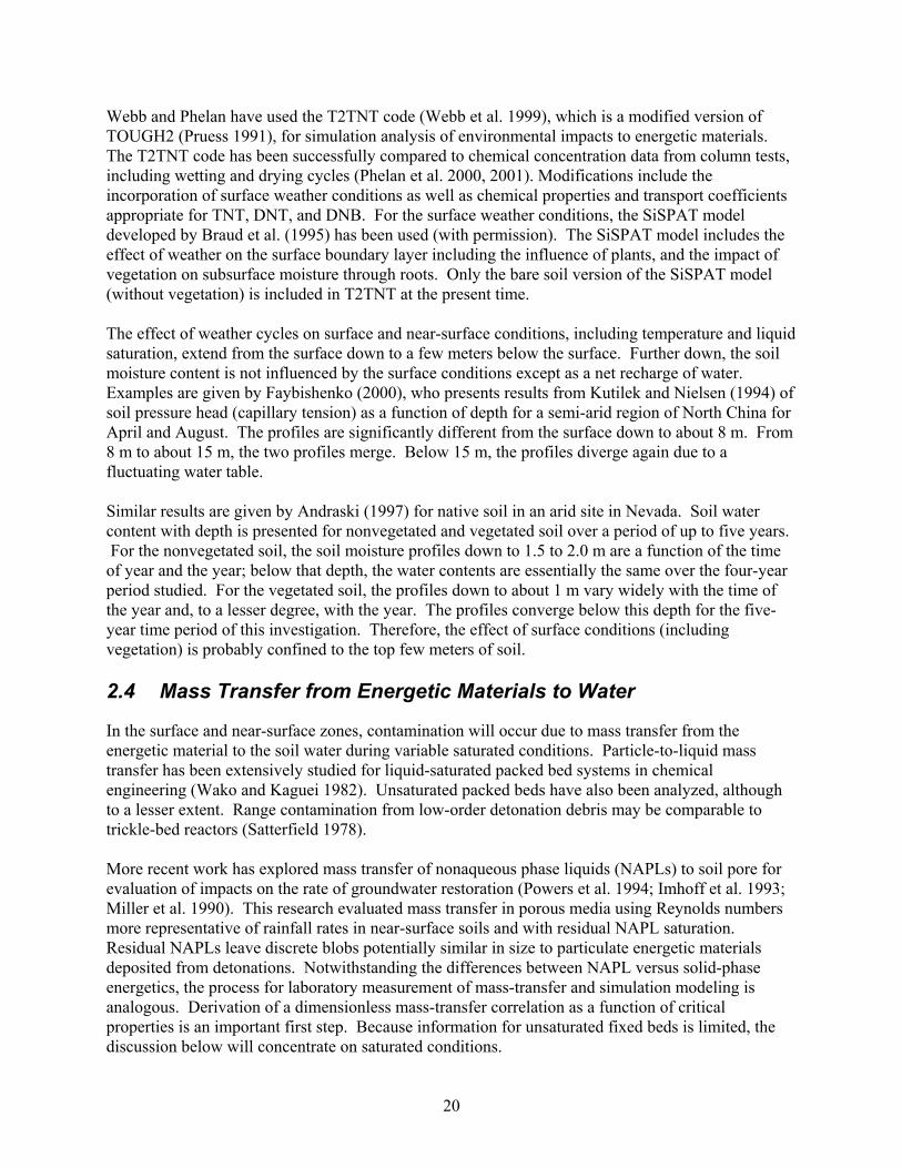
Traditional field-soil sampling and chemical residue analysis is often unable to determine the presence of solid-phase energetic material. The soil extraction and analyte determination process averages the measured energetic material quantity over the entire mass of the soil sample, masking the potential presence of small particles of energetic material. Estimating the transition from classical soil chemical residues based on sorption equilibria to the potential presence of a separate solid-phase energetic material may be important in the selection and use of appropriate fate and transport analysis tools. One method to estimate the transition of trace soil residues to the potential presence of solid-phase energetics is through evaluation of phase-partitioning equilibria (Jury 1991; Phelan and Barnett 2001). A soil system will partition the total mass of chemicals between the air, water and solid phases according to equilibrium partitioning theory. The mass fraction in each soil phase is established by the air-water partition (Henry’s Constant), the soil-water partition (Kd) and soil-air partition (Kd’) coefficients. The greater the total soil residue (among all soil phases), the greater the concentration in each of the soil phases. However, when the total soil residue approaches a value that, when partitioned, approaches the water solubility limit, any additional mass added to the system must partition into a separate solid phase. Total soil concentrations that do not exceed the partitioning equilibria will behave as a traditional pollutant. Total soil concentrations that exceed this value may require analysis tools that include the behavior of a separate solid phase. Figure 4 presents the results of an analysis that shows the maximum total soil concentrations of RDX that a soil can partition before a separate solid phase must exist. At 20°C, the maximum solubility of RDX in water is about 45 mg/L. Due to the low vapor pressure and air-water partitioning coefficient, the soil-water partition coefficient (Kd) is the principal factor influencing the maximum total soil residue. Figure 4 shows that total soil concentrations above 30 to 70 μg/g (sum of liquid, sorbed to soil and vapor phases) indicate the potential presence of solid phase energetics in the soil.
Yellow solid
19
The lower the soil-water partitioning coefficient (Kd) the lower the maximum total soil residue because of the smaller sorption capacity of the soil.
0
5
10
15
20
25
30
35
40
45
50
0 10 20 30 40 50 60 70 80 90 100
Total Soil Concentration (ug/g)
Pore
Wat
er C
once
ntra
tion
(mg/
L)
T = 20 oCSl = 99 %
Maximum Water Solubility
Kd = 0.1 mL/g
Kd = 0.3 mL/g
Kd = 1.0 mL/g
Figure 4. Effect of Soil Water Partitioning Coefficient (Kd) on Maximum Soil Residue for RDX
2.3 Importance of Surface Conditions
Leaching of energetic material from detonation debris is likely to be controlled by surface weather phenomena. These materials are found on and in near-surface soils, where large changes in temperature, pore-water velocity and soil saturation occur. Higher temperatures increase the solubility of the energetic material in water. Increased pore-water velocity may increase the mass transfer rate and a higher water flux will increase the mass of contaminated water. Increased saturation fills more pore space, potentially increasing contact with the energetic material. The soil surface temperature has a strong diurnal variation due to the balance of solar radiation, long-wave radiation, heat conduction into the soil, and evaporation. For example, the diurnal variation for a bare soil in a dry climate has been measured to be between 15°C and 50°C with an approximately sinusoidal variation (Braud et al. 1993). The solubility data for RDX shows a change in solubility of about a factor five for this temperature range (Phelan et al. 2002). The soil surface and near-surface conditions, such as the temperature, saturation, and evaporation, are driven by local weather conditions including pressure, air temperature, relative humidity, wind speed, solar radiation, long-wave radiation, and precipitation. Webb and Phelan (2000) modeled the effect of diurnal and seasonal weather on the surface and near-surface TNT, dinitrotoluene (DNT), and dinitrobenzene (DNB) chemical signatures from a constant source release simulation of a buried landmine or unexploded ordnance (UXO). Liquid-phase chemical concentrations showed about a 2-order-of-magnitude diurnal variation under dry conditions, and about an 8-order-of-magnitude range over the entire year. Therefore, the effect of weather conditions on chemical concentrations of energetic materials is expected to be significant.
20
Webb and Phelan have used the T2TNT code (Webb et al. 1999), which is a modified version of TOUGH2 (Pruess 1991), for simulation analysis of environmental impacts to energetic materials. The T2TNT code has been successfully compared to chemical concentration data from column tests, including wetting and drying cycles (Phelan et al. 2000, 2001). Modifications include the incorporation of surface weather conditions as well as chemical properties and transport coefficients appropriate for TNT, DNT, and DNB. For the surface weather conditions, the SiSPAT model developed by Braud et al. (1995) has been used (with permission). The SiSPAT model includes the effect of weather on the surface boundary layer including the influence of plants, and the impact of vegetation on subsurface moisture through roots. Only the bare soil version of the SiSPAT model (without vegetation) is included in T2TNT at the present time. The effect of weather cycles on surface and near-surface conditions, including temperature and liquid saturation, extend from the surface down to a few meters below the surface. Further down, the soil moisture content is not influenced by the surface conditions except as a net recharge of water. Examples are given by Faybishenko (2000), who presents results from Kutilek and Nielsen (1994) of soil pressure head (capillary tension) as a function of depth for a semi-arid region of North China for April and August. The profiles are significantly different from the surface down to about 8 m. From 8 m to about 15 m, the two profiles merge. Below 15 m, the profiles diverge again due to a fluctuating water table. Similar results are given by Andraski (1997) for native soil in an arid site in Nevada. Soil water content with depth is presented for nonvegetated and vegetated soil over a period of up to five years. For the nonvegetated soil, the soil moisture profiles down to 1.5 to 2.0 m are a function of the time of year and the year; below that depth, the water contents are essentially the same over the four-year period studied. For the vegetated soil, the profiles down to about 1 m vary widely with the time of the year and, to a lesser degree, with the year. The profiles converge below this depth for the five-year time period of this investigation. Therefore, the effect of surface conditions (including vegetation) is probably confined to the top few meters of soil. 2.4 Mass Transfer from Energetic Materials to Water
In the surface and near-surface zones, contamination will occur due to mass transfer from the energetic material to the soil water during variable saturated conditions. Particle-to-liquid mass transfer has been extensively studied for liquid-saturated packed bed systems in chemical engineering (Wako and Kaguei 1982). Unsaturated packed beds have also been analyzed, although to a lesser extent. Range contamination from low-order detonation debris may be comparable to trickle-bed reactors (Satterfield 1978). More recent work has explored mass transfer of nonaqueous phase liquids (NAPLs) to soil pore for evaluation of impacts on the rate of groundwater restoration (Powers et al. 1994; Imhoff et al. 1993; Miller et al. 1990). This research evaluated mass transfer in porous media using Reynolds numbers more representative of rainfall rates in near-surface soils and with residual NAPL saturation. Residual NAPLs leave discrete blobs potentially similar in size to particulate energetic materials deposited from detonations. Notwithstanding the differences between NAPL versus solid-phase energetics, the process for laboratory measurement of mass-transfer and simulation modeling is analogous. Derivation of a dimensionless mass-transfer correlation as a function of critical properties is an important first step. Because information for unsaturated fixed beds is limited, the discussion below will concentrate on saturated conditions.
21
In these packed-bed systems, the Sherwood number is usually correlated with the Reynolds number. The Sherwood number is a dimensionless parameter, or
(Re)fDDk
Shv
p =⋅
= [1]
where k is the mass transfer rate from the particle, Dp is the particle diameter, and Dv is the diffusion coefficient. The Reynolds number is the ratio of the fluid velocity times the particle diameter divided by the fluid viscosity. In many situations, such as NAPL dissolution as given by Powers et al. (1992), the interfacial area of the mass source is not measured, and a modified Sherwood number, Sh*, can be defined using a lumped mass transfer coefficient (k* = k a), or
v
p
DDk
Sh2
* ⋅= [2]
where a is the specific surface area. The lumped mass in transfer coefficient can then be evaluated directly from the effluent concentration from a column flow-test apparatus. While soils contain a wide range of particle diameters, an average or mean particle size is sometimes employed for Reynolds number calculations. Using a 1-mm mean grain size and a rainfall rate (or net recharge) of 1 cm/day, the Reynolds number is very low, about 10-4. Models for the mass-transfer rates (modified Sherwood number) from NAPLs under saturated flow conditions with these low Reynolds numbers (Re < 1) have been developed by a number of authors, including Powers et al. (1992, 1994) and Imhoff et al. (1993). NAPL dissolution behavior is not entirely analogous to energetic materials because the NAPL is a liquid and the size of the NAPL “particles” will be determined by the soil particle size distribution. The above relationships may not apply directly to the present situation due to a number of factors. First of all, these relationships are derived for saturated flow conditions. For unsaturated flow, few investigations have been conducted. Based on a preliminary analysis of heat transfer in unsaturated flow, the results of Plumb (1991) indicate that the heat transfer coefficient is approximately proportional to the liquid saturation. By analogy, mass transfer can be assumed to be proportional to the liquid saturation. As mentioned above, NAPL “particle” sizes will be influenced by the soil-pore size distribution, which will not be the case for energetic particles. Sorption and degradation losses involving energetic particles and the soil may further complicate experimental determination of the mass transfer rate, which may be avoided by using a synthetic soil made from glass beads.

22
23
3. Project Plan This project has been divided into two tasks, Experimental and Modeling, as follows: 3.1 Task 1: Experimental
Measurement of mass transfer from solid particles to water has been performed predominantly with packed-bed reactors in support of chemical engineering operations research (Wakao and Kaguei 1982) and with NAPLs in porous media (Powers et al. 1994). Experimental design for this application was patterned after this previous work. The principal parameters that control the mass transfer rate include:
• Soil saturation • Porous medium particle size distribution • Fluid flow rate • Energetic material surface area • Temperature • Buried or surface deposit • Steady or pulsed flow • Energetic material type
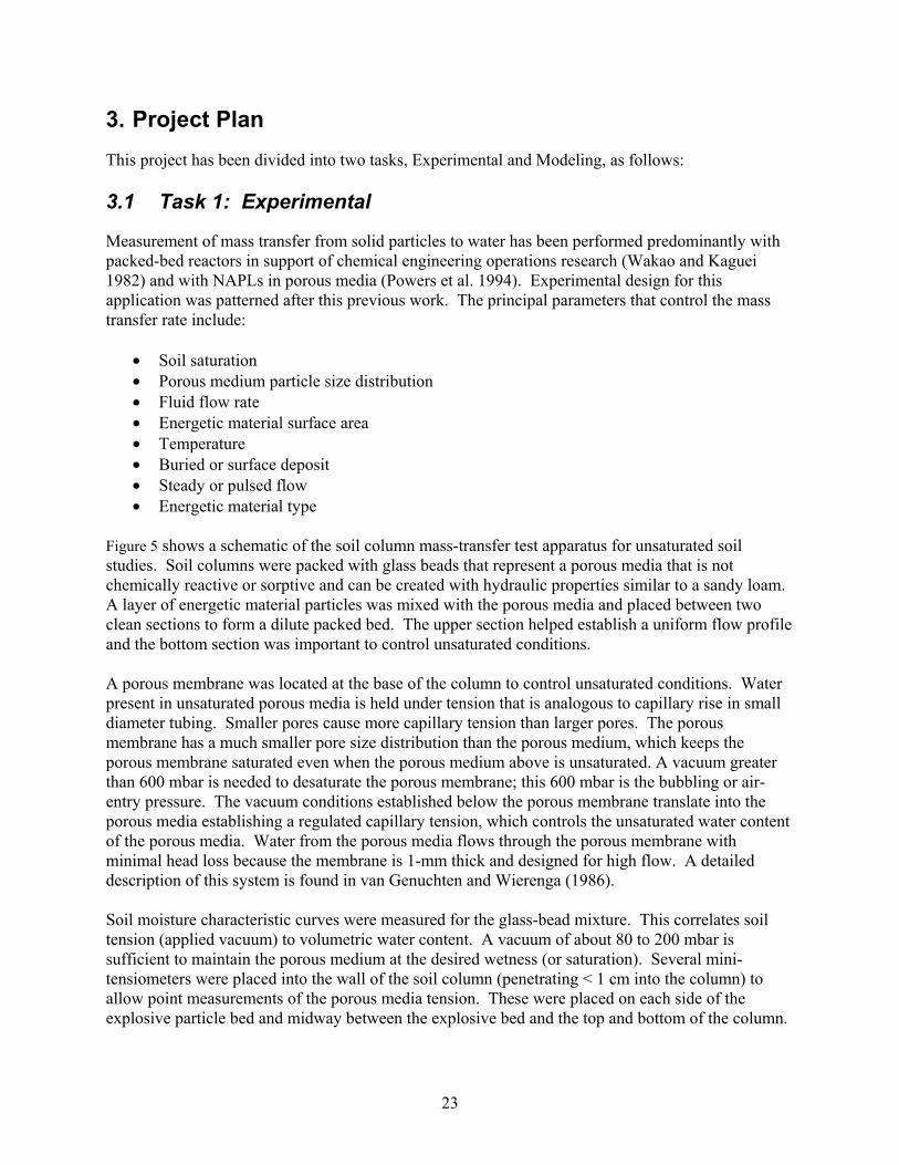
Figure 5 shows a schematic of the soil column mass-transfer test apparatus for unsaturated soil studies. Soil columns were packed with glass beads that represent a porous media that is not chemically reactive or sorptive and can be created with hydraulic properties similar to a sandy loam. A layer of energetic material particles was mixed with the porous media and placed between two clean sections to form a dilute packed bed. The upper section helped establish a uniform flow profile and the bottom section was important to control unsaturated conditions. A porous membrane was located at the base of the column to control unsaturated conditions. Water present in unsaturated porous media is held under tension that is analogous to capillary rise in small diameter tubing. Smaller pores cause more capillary tension than larger pores. The porous membrane has a much smaller pore size distribution than the porous medium, which keeps the porous membrane saturated even when the porous medium above is unsaturated. A vacuum greater than 600 mbar is needed to desaturate the porous membrane; this 600 mbar is the bubbling or air-entry pressure. The vacuum conditions established below the porous membrane translate into the porous media establishing a regulated capillary tension, which controls the unsaturated water content of the porous media. Water from the porous media flows through the porous membrane with minimal head loss because the membrane is 1-mm thick and designed for high flow. A detailed description of this system is found in van Genuchten and Wierenga (1986). Soil moisture characteristic curves were measured for the glass-bead mixture. This correlates soil tension (applied vacuum) to volumetric water content. A vacuum of about 80 to 200 mbar is sufficient to maintain the porous medium at the desired wetness (or saturation). Several mini-tensiometers were placed into the wall of the soil column (penetrating < 1 cm into the column) to allow point measurements of the porous media tension. These were placed on each side of the explosive particle bed and midway between the explosive bed and the top and bottom of the column.
24
Water samples were collected in a fraction collector set to optimize the number of samples per day depending on the set water inflow rate. Time sequenced sample collection allows an evaluation of the time-dependent behavior of the mass transfer. Water samples were analyzed by Reverse Phase High Performance Liquid Chromatography optimized for RDX and TNT elution times. U.S. Military Composition B (Comp B) was used as the principal source material to allow data collection for both RDX and TNT in a formulation commonly used in military training operations. RDX is likely to have the greatest threat to groundwater as it has the lowest drinking water advisory (McLellan et al. 1988), sorbs poorly to soils (Singh 1988), and has a low degradation rate under typical aerobic vadose zone pore water conditions (Hawari, J. 2000).
Figure 5. Laboratory Experimental Apparatus
The tests involved three phases of experimentation and model development.
• Phase I consisted of an initial series of experiments designed to determine the critical parameters affecting the mass transfer of energetic materials to pore water and the derivation of a mathematical function that incorporated the most significant factors.
• Phase II evaluated in more detail the factors that have the greatest impact in the mass-transfer process and began to evaluate actual post-blast residue with soil obtained from a test and training range. This will allow a comparison of artificial glass beads containing manufactured explosive particles with more realistic conditions found in the field.
• Phase III explored the effect of particle size, whether a surface deposit differed from a buried deposit, and additional low-order detonation debris.
PeristalticPump
T1T5 T4 T3 T2
Energetic Material
FractionCollector
SimulatedRainwater
Temperature Cell
Glass Beads or Soil
T6
To Vacuum
Porous Plate
25
3.2 Task 2: Modeling
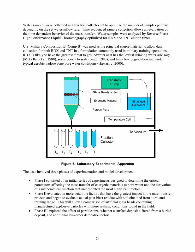
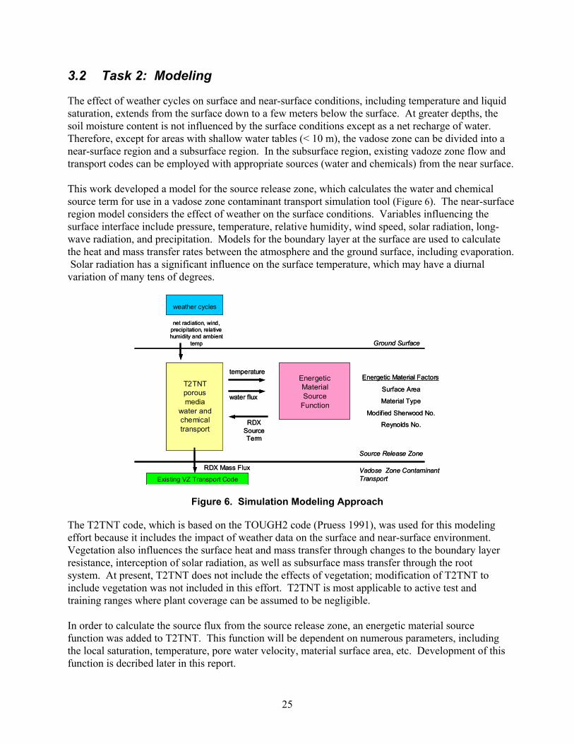
The effect of weather cycles on surface and near-surface conditions, including temperature and liquid saturation, extends from the surface down to a few meters below the surface. At greater depths, the soil moisture content is not influenced by the surface conditions except as a net recharge of water. Therefore, except for areas with shallow water tables (< 10 m), the vadose zone can be divided into a near-surface region and a subsurface region. In the subsurface region, existing vadoze zone flow and transport codes can be employed with appropriate sources (water and chemicals) from the near surface. This work developed a model for the source release zone, which calculates the water and chemical source term for use in a vadose zone contaminant transport simulation tool (Figure 6). The near-surface region model considers the effect of weather on the surface conditions. Variables influencing the surface interface include pressure, temperature, relative humidity, wind speed, solar radiation, long-wave radiation, and precipitation. Models for the boundary layer at the surface are used to calculate the heat and mass transfer rates between the atmosphere and the ground surface, including evaporation. Solar radiation has a significant influence on the surface temperature, which may have a diurnal variation of many tens of degrees.
weather cycles
net radiation, wind, precipitation, relative humidity and ambient
temp
T2TNT porous media
water and chemical transport
temperatureEnergetic Material Source
Function
RDX Source Term
RDX Mass Flux
water flux
Energetic Material Factors
Surface Area
Material Type
Modified Sherwood No.
Reynolds No.
Ground Surface
Source Release Zone
Vadose Zone Contaminant TransportExisting VZ Transport Code
Figure 6. Simulation Modeling Approach
The T2TNT code, which is based on the TOUGH2 code (Pruess 1991), was used for this modeling effort because it includes the impact of weather data on the surface and near-surface environment. Vegetation also influences the surface heat and mass transfer through changes to the boundary layer resistance, interception of solar radiation, as well as subsurface mass transfer through the root system. At present, T2TNT does not include the effects of vegetation; modification of T2TNT to include vegetation was not included in this effort. T2TNT is most applicable to active test and training ranges where plant coverage can be assumed to be negligible. In order to calculate the source flux from the source release zone, an energetic material source function was added to T2TNT. This function will be dependent on numerous parameters, including the local saturation, temperature, pore water velocity, material surface area, etc. Development of this function is decribed later in this report.

26
27
4. Experimental Methods
4.1 Test Plans
Test plans were developed in the project proposal based on best judgment of the most important controlling factors. As the tests were completed, subsequent tests were designed to assess certain factors in more detail. Forty distinct tests were successfully completed. Table 3 shows the factors explored in each test phase and group.
Table 3. Experimental Test Phases and Principal Factors
Test Phase Principal Factors Mass Transfer Test Designator
Phase I, Test Group A Flow, temperature, EM particle size MT1, MT2, MT3
Phase I, Test Group B Porous media saturation MT5, MT12
Phase II, Test Group A Bed loading, bed depth, initial wetting rate
MT6, MT7, MT8, MT8b, MT8c, MT8d, MT9b2, 9b3
Phase II, Test Group B Flow, EM particle size, detonation debris
MT10, MT13, MT14, MT11, MT15, MT16, MT17, MT18
Phase III Surface vs. buried deposits, EM particle size, low order detonation debris
MT19-1, 2, 3, 4; MT20-1, 2, 3; MT21-1, 2; MT22-1, 2, 3; MT23-1, 2; MT24-1; MT25-1; MT26-1, MT27-1; MT28-1.
4.2 Chemical Analysis
4.2.1 High-Pressure Liquid Chromatography (HPLC) Method
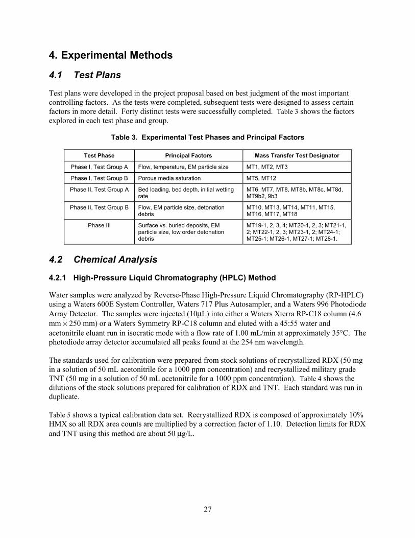
Water samples were analyzed by Reverse-Phase High-Pressure Liquid Chromatography (RP-HPLC) using a Waters 600E System Controller, Waters 717 Plus Autosampler, and a Waters 996 Photodiode Array Detector. The samples were injected (10μL) into either a Waters Xterra RP-C18 column (4.6 mm × 250 mm) or a Waters Symmetry RP-C18 column and eluted with a 45:55 water and acetonitrile eluant run in isocratic mode with a flow rate of 1.00 mL/min at approximately 35°C. The photodiode array detector accumulated all peaks found at the 254 nm wavelength. The standards used for calibration were prepared from stock solutions of recrystallized RDX (50 mg in a solution of 50 mL acetonitrile for a 1000 ppm concentration) and recrystallized military grade TNT (50 mg in a solution of 50 mL acetonitrile for a 1000 ppm concentration). Table 4 shows the dilutions of the stock solutions prepared for calibration of RDX and TNT. Each standard was run in duplicate. Table 5 shows a typical calibration data set. Recrystallized RDX is composed of approximately 10% HMX so all RDX area counts are multiplied by a correction factor of 1.10. Detection limits for RDX and TNT using this method are about 50 μg/L.
28
Table 4. RDX and TNT Standard Compositions
40 μL RDX solution 100 μL TNT solution 860μL distilled water 40 ppm RDX 100 ppm TNT
30 μL RDX solution 80 μL TNT solution 890 μL distilled water 30 ppm RDX 80 ppm TNT
20 μL RDX solution 60 μL TNT solution 920 μL distilled water 20 ppm RDX 60 ppm TNT
10 μL RDX solution 40 μL TNT solution 950 μL distilled water 10 ppm RDX 40 ppm TNT
5 μL RDX solution 20 μL TNT solution 975 μL distilled water 5 ppm RDX 20 ppm TNT
Table 5. Calibration Chart for RDX and TNT Standards
RDX Standard (ppm) Area TNT
Standard (ppm) Area
40 618392 100 3323126 40 617110 100 3315721 30 463950.5 80 2641996 30 464988.2 80 2636602 20 308603 60 1988464 20 308652.5 60 1989367 10 154020 40 1328480 10 152578 40 1325699 5 83437.69 20 652792 5 83570.84 20 653216
Slope 15460.23 Slope 33116.58 R2 0.999851 R2 0.99995
Each fraction collector sample was weighed in its container (an 8 mL glass test tube). The tare weight of an empty vial was subtracted to determine the effluent mass of each sample. A 1 mL subsample was collected by disposable pipette, placed in a 2 mL amber autosampler vial. Analysis routines used a calibration check sample every 10 sample runs to verify analyte recovery between 90 and 110%. Recalibration was necessary about every two to four weeks. 4.3 Energetic Material
4.3.1 Comp B Source Material
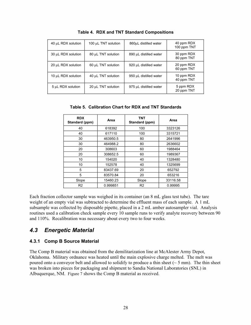
The Comp B material was obtained from the demilitarization line at McAlester Army Depot, Oklahoma. Military ordnance was heated until the main explosive charge melted. The melt was poured onto a conveyor belt and allowed to solidify to produce a thin sheet (~ 5 mm). The thin sheet was broken into pieces for packaging and shipment to Sandia National Laboratories (SNL) in Albuquerque, NM. Figure 7 shows the Comp B material as received.
29
Figure 7. Comp B Starting Material
4.3.1.1 Physical/Chemical Properties
The Comp B was further reduced in size by first freezing in liquid nitrogen and then placing it into a ball mill which was rotated for 1 hour at ~ 60 revolutions per minute. The broken material from the ball mill was placed into a sieve shaker, including the zirconium oxide balls, with the sieves as shown in Table 6 and shaken for 1 hour. Size fractions were collected and the shaker operated for another three cycles.
Table 6. Sieve Series
Sieve Number Opening (μm)
16 1180
18 1000
30 600
35 500
140 106
170 90
635 20
Approximately 500 g of Comp B was processed. Size fractions containing 1000 to 1180 μm, 500 to 600 μm and 90 to 106 μm were collected. There was very little material in the less than 20 μm fraction. To quantify the fraction of RDX and TNT in each Comp B size separate, ca. 0.010 g (± 0.0001 g) was dissolved into 10 mL of acetonitrile, diluted 1:1 with water and quantified using the RP-HPLC as described above. The results of the mass fraction of RDX and TNT in each size separate are shown in Table 7.
Composition B Zirconium Oxide Balls
30
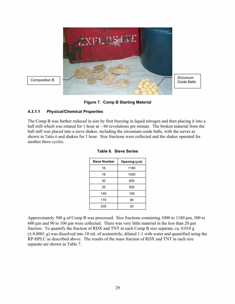
Table 7. RDX and TNT Mass Fraction in Each Size Separate
Component 90 to 106 μm 500 to 600 μm 1000 to 1180 μm
RDX 0.546 0.598 0.579
TNT 0.454 0.402 0.421
These results indicate that the Comp B size separates remained near the typical 60/40-blend ratio, with slightly lower ratio for the 90 to 106 μm size separate. The specific surface area of each size separate was measured using a Micromeritics Accelerated Surface Area and Porosimetry 2405 Instrument that measures BET (Brunauer, Emmett, and Teller) surface area with Kr gas. The results for the BET-specific surface area measurements are shown in Table 8 along with estimates based on the geometry of a spherical particle.
Table 8. Specific Surface Area of Comp B Size Separates
Size Fraction BET Single Point (m2/g)
BET Multi Point (m2/g)
Spherical Calculated (m2/g)
90 to 106 μm 0.3283 0.4961 (± 0.0052) 0.0371
500 to 600 μm 0.1566 0.2071 (± 0.0013) 0.0066
1000 to 1180 μm 0.1750 0.2293 (± 0.0012) 0.0033
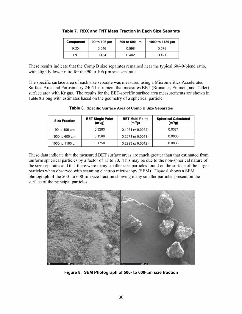
These data indicate that the measured BET surface areas are much greater than that estimated from uniform spherical particles by a factor of 13 to 70. This may be due to the non-spherical nature of the size separates and that there were many smaller-size particles found on the surface of the larger particles when observed with scanning electron microscopy (SEM). Figure 8 shows a SEM photograph of the 500- to 600-μm size fraction showing many smaller particles present on the surface of the principal particles.
Figure 8. SEM Photograph of 500- to 600-μm size fraction
31
4.3.2 Low-Order Detonation Debris
Two sets of low-order detonation debris were provided by the companion project to this effort - SERDP Project CP-1155 at the US Army Engineer Research and Development Center. (Pennington et al. 2003, Taylor et al. 2004). 4.3.2.1 First Set of Tests
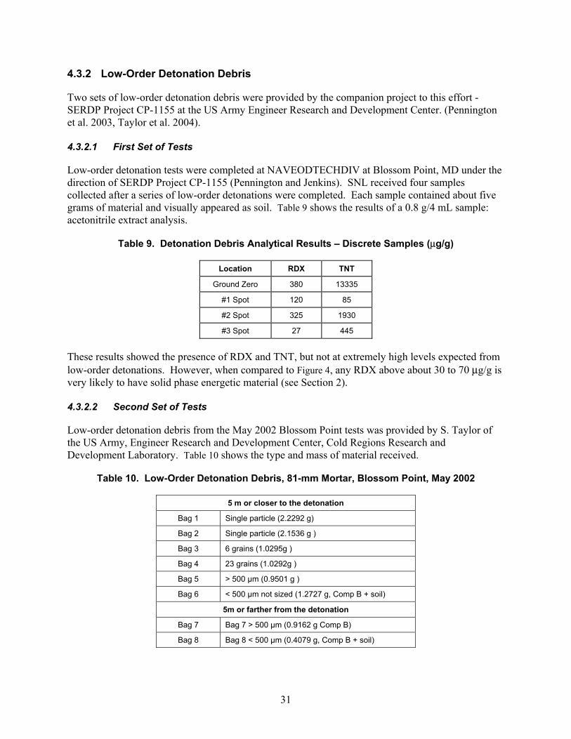
Low-order detonation tests were completed at NAVEODTECHDIV at Blossom Point, MD under the direction of SERDP Project CP-1155 (Pennington and Jenkins). SNL received four samples collected after a series of low-order detonations were completed. Each sample contained about five grams of material and visually appeared as soil. Table 9 shows the results of a 0.8 g/4 mL sample: acetonitrile extract analysis.
Table 9. Detonation Debris Analytical Results – Discrete Samples (μg/g)
Location RDX TNT
Ground Zero 380 13335
#1 Spot 120 85
#2 Spot 325 1930
#3 Spot 27 445
These results showed the presence of RDX and TNT, but not at extremely high levels expected from low-order detonations. However, when compared to Figure 4, any RDX above about 30 to 70 μg/g is very likely to have solid phase energetic material (see Section 2). 4.3.2.2 Second Set of Tests
Low-order detonation debris from the May 2002 Blossom Point tests was provided by S. Taylor of the US Army, Engineer Research and Development Center, Cold Regions Research and Development Laboratory. Table 10 shows the type and mass of material received.
Table 10. Low-Order Detonation Debris, 81-mm Mortar, Blossom Point, May 2002
5 m or closer to the detonation
Bag 1 Single particle (2.2292 g)
Bag 2 Single particle (2.1536 g )
Bag 3 6 grains (1.0295g )
Bag 4 23 grains (1.0292g )
Bag 5 > 500 µm (0.9501 g )
Bag 6 < 500 µm not sized (1.2727 g, Comp B + soil)
5m or farther from the detonation
Bag 7 Bag 7 > 500 µm (0.9162 g Comp B)
Bag 8 Bag 8 < 500 µm (0.4079 g, Comp B + soil)
32
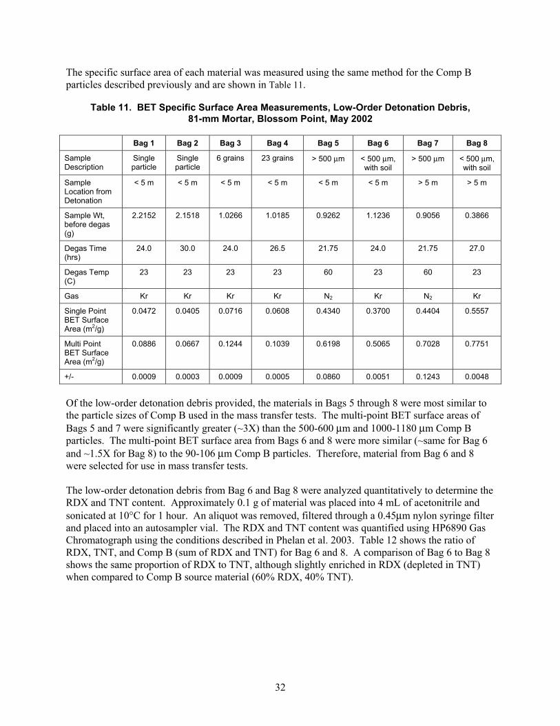
The specific surface area of each material was measured using the same method for the Comp B particles described previously and are shown in Table 11.
Table 11. BET Specific Surface Area Measurements, Low-Order Detonation Debris, 81-mm Mortar, Blossom Point, May 2002
Bag 1 Bag 2 Bag 3 Bag 4 Bag 5 Bag 6 Bag 7 Bag 8
Sample Description
Single particle
Single particle
6 grains 23 grains > 500 μm < 500 μm, with soil
> 500 μm < 500 μm, with soil
Sample Location from Detonation
< 5 m < 5 m < 5 m < 5 m < 5 m < 5 m > 5 m > 5 m
Sample Wt, before degas (g)
2.2152 2.1518 1.0266 1.0185 0.9262 1.1236 0.9056 0.3866
Degas Time (hrs)
24.0 30.0 24.0 26.5 21.75 24.0 21.75 27.0
Degas Temp (C)
23 23 23 23 60 23 60 23
Gas Kr Kr Kr Kr N2 Kr N2 Kr
Single Point BET Surface Area (m2/g)
0.0472 0.0405 0.0716 0.0608 0.4340 0.3700 0.4404 0.5557
Multi Point BET Surface Area (m2/g)
0.0886 0.0667 0.1244 0.1039 0.6198 0.5065 0.7028 0.7751
+/- 0.0009 0.0003 0.0009 0.0005 0.0860 0.0051 0.1243 0.0048
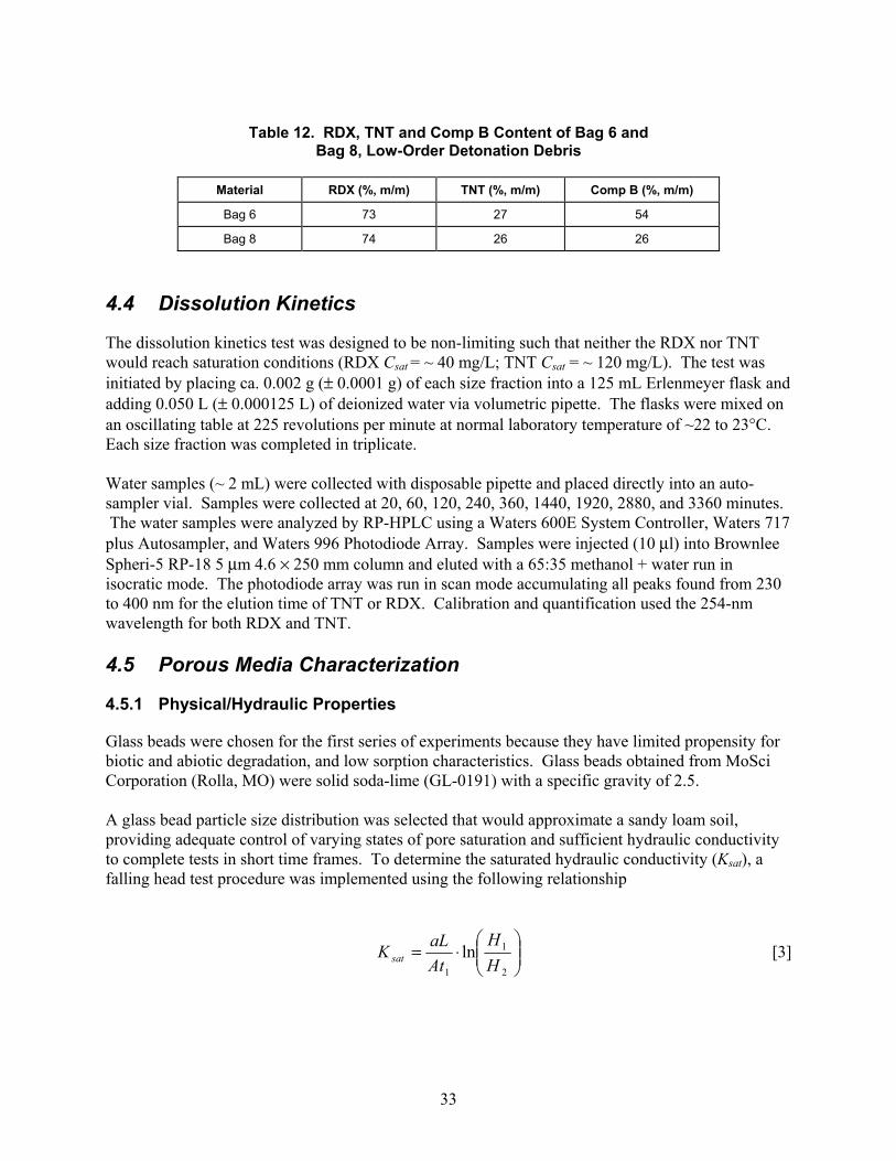
Of the low-order detonation debris provided, the materials in Bags 5 through 8 were most similar to the particle sizes of Comp B used in the mass transfer tests. The multi-point BET surface areas of Bags 5 and 7 were significantly greater (~3X) than the 500-600 μm and 1000-1180 μm Comp B particles. The multi-point BET surface area from Bags 6 and 8 were more similar (~same for Bag 6 and ~1.5X for Bag 8) to the 90-106 μm Comp B particles. Therefore, material from Bag 6 and 8 were selected for use in mass transfer tests. The low-order detonation debris from Bag 6 and Bag 8 were analyzed quantitatively to determine the RDX and TNT content. Approximately 0.1 g of material was placed into 4 mL of acetonitrile and sonicated at 10°C for 1 hour. An aliquot was removed, filtered through a 0.45μm nylon syringe filter and placed into an autosampler vial. The RDX and TNT content was quantified using HP6890 Gas Chromatograph using the conditions described in Phelan et al. 2003. Table 12 shows the ratio of RDX, TNT, and Comp B (sum of RDX and TNT) for Bag 6 and 8. A comparison of Bag 6 to Bag 8 shows the same proportion of RDX to TNT, although slightly enriched in RDX (depleted in TNT) when compared to Comp B source material (60% RDX, 40% TNT).
33
Table 12. RDX, TNT and Comp B Content of Bag 6 and Bag 8, Low-Order Detonation Debris
Material RDX (%, m/m) TNT (%, m/m) Comp B (%, m/m)
Bag 6 73 27 54
Bag 8 74 26 26
4.4 Dissolution Kinetics
The dissolution kinetics test was designed to be non-limiting such that neither the RDX nor TNT would reach saturation conditions (RDX Csat = ~ 40 mg/L; TNT Csat = ~ 120 mg/L). The test was initiated by placing ca. 0.002 g (± 0.0001 g) of each size fraction into a 125 mL Erlenmeyer flask and adding 0.050 L (± 0.000125 L) of deionized water via volumetric pipette. The flasks were mixed on an oscillating table at 225 revolutions per minute at normal laboratory temperature of ~22 to 23°C. Each size fraction was completed in triplicate. Water samples (~ 2 mL) were collected with disposable pipette and placed directly into an auto-sampler vial. Samples were collected at 20, 60, 120, 240, 360, 1440, 1920, 2880, and 3360 minutes. The water samples were analyzed by RP-HPLC using a Waters 600E System Controller, Waters 717 plus Autosampler, and Waters 996 Photodiode Array. Samples were injected (10 μl) into Brownlee Spheri-5 RP-18 5 μm 4.6 × 250 mm column and eluted with a 65:35 methanol + water run in isocratic mode. The photodiode array was run in scan mode accumulating all peaks found from 230 to 400 nm for the elution time of TNT or RDX. Calibration and quantification used the 254-nm wavelength for both RDX and TNT. 4.5 Porous Media Characterization
4.5.1 Physical/Hydraulic Properties
Glass beads were chosen for the first series of experiments because they have limited propensity for biotic and abiotic degradation, and low sorption characteristics. Glass beads obtained from MoSci Corporation (Rolla, MO) were solid soda-lime (GL-0191) with a specific gravity of 2.5. A glass bead particle size distribution was selected that would approximate a sandy loam soil, providing adequate control of varying states of pore saturation and sufficient hydraulic conductivity to complete tests in short time frames. To determine the saturated hydraulic conductivity (Ksat), a falling head test procedure was implemented using the following relationship
⎟⎟⎠
⎞⎜⎜⎝
⎛⋅=
2
1
1
lnHH
AtaLK sat [3]
34
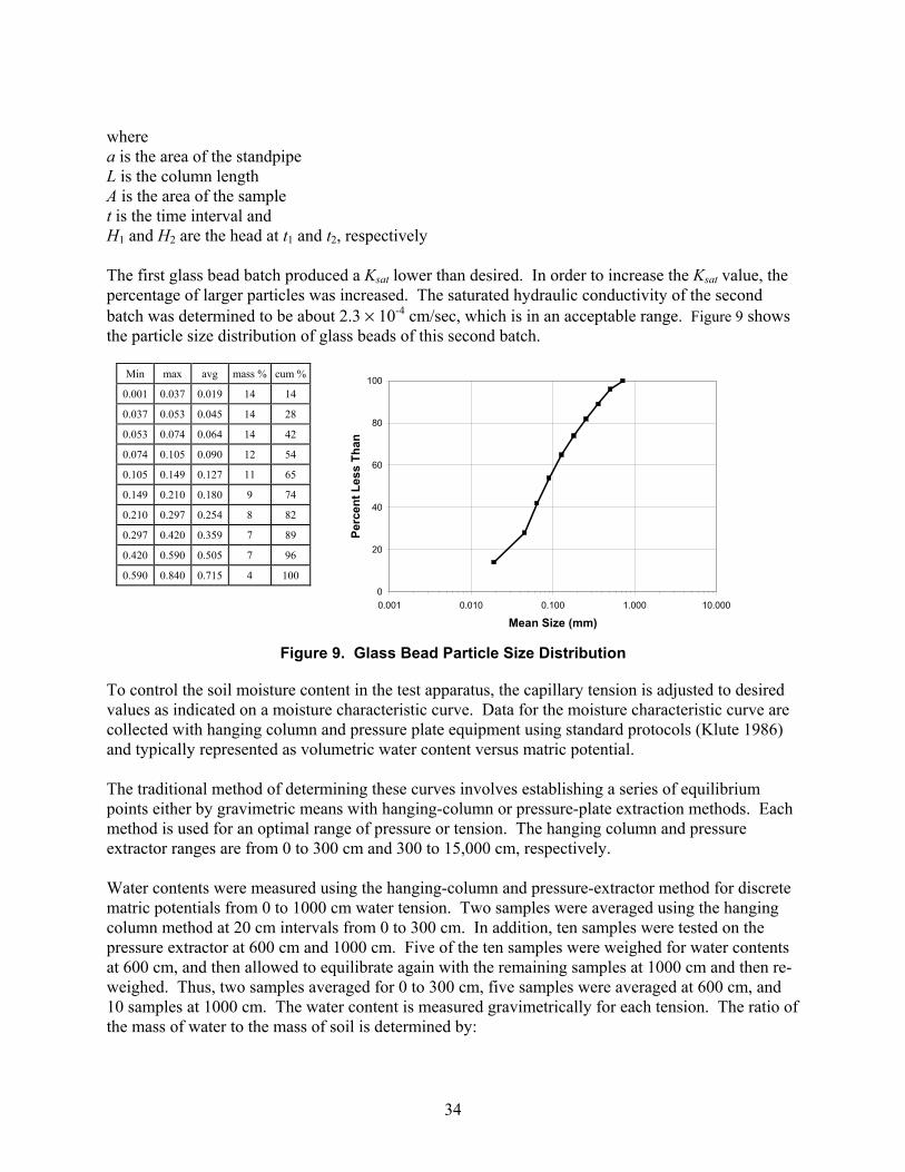
where a is the area of the standpipe L is the column length A is the area of the sample t is the time interval and H1 and H2 are the head at t1 and t2, respectively The first glass bead batch produced a Ksat lower than desired. In order to increase the Ksat value, the percentage of larger particles was increased. The saturated hydraulic conductivity of the second batch was determined to be about 2.3 × 10⁻⁴ cm/sec, which is in an acceptable range. Figure 9 shows the particle size distribution of glass beads of this second batch.
Min max avg mass % cum %
0.001 0.037 0.019 14 14
0.037 0.053 0.045 14 28
0.053 0.074 0.064 14 42
0.074 0.105 0.090 12 54
0.105 0.149 0.127 11 65
0.149 0.210 0.180 9 74
0.210 0.297 0.254 8 82
0.297 0.420 0.359 7 89
0.420 0.590 0.505 7 96
0.590 0.840 0.715 4 100
Figure 9. Glass Bead Particle Size Distribution
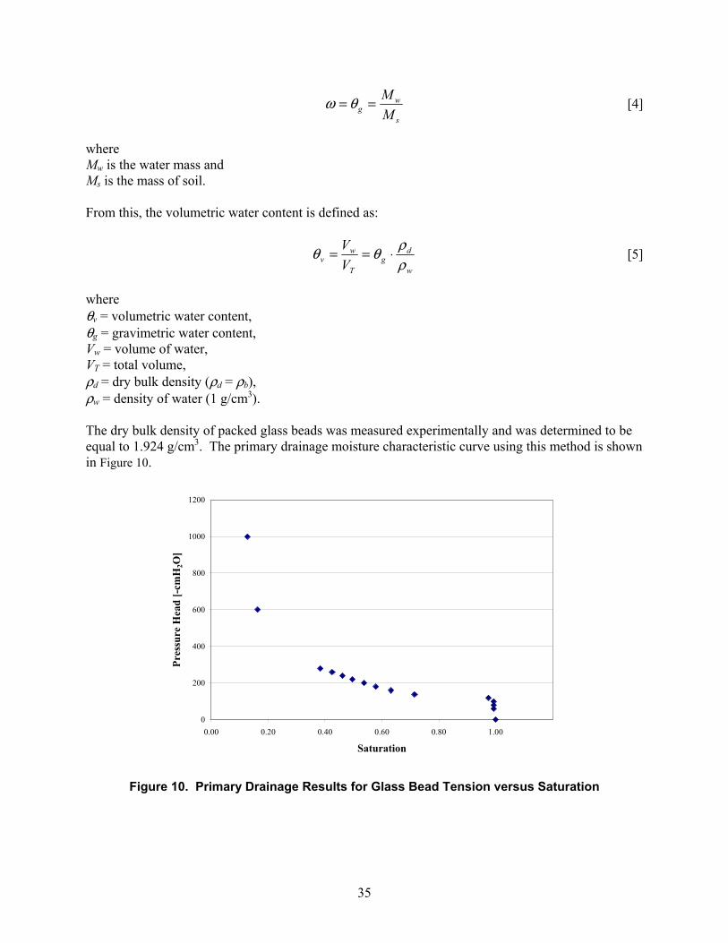
To control the soil moisture content in the test apparatus, the capillary tension is adjusted to desired values as indicated on a moisture characteristic curve. Data for the moisture characteristic curve are collected with hanging column and pressure plate equipment using standard protocols (Klute 1986) and typically represented as volumetric water content versus matric potential. The traditional method of determining these curves involves establishing a series of equilibrium points either by gravimetric means with hanging-column or pressure-plate extraction methods. Each method is used for an optimal range of pressure or tension. The hanging column and pressure extractor ranges are from 0 to 300 cm and 300 to 15,000 cm, respectively. Water contents were measured using the hanging-column and pressure-extractor method for discrete matric potentials from 0 to 1000 cm water tension. Two samples were averaged using the hanging column method at 20 cm intervals from 0 to 300 cm. In addition, ten samples were tested on the pressure extractor at 600 cm and 1000 cm. Five of the ten samples were weighed for water contents at 600 cm, and then allowed to equilibrate again with the remaining samples at 1000 cm and then re-weighed. Thus, two samples averaged for 0 to 300 cm, five samples were averaged at 600 cm, and 10 samples at 1000 cm. The water content is measured gravimetrically for each tension. The ratio of the mass of water to the mass of soil is determined by:
0
20
40
60
80
100
0.001 0.010 0.100 1.000 10.000
Mean Size (mm)
Perc
ent L
ess
Than
35
s
wg M
M== θω [4]
where Mw is the water mass and Ms is the mass of soil. From this, the volumetric water content is defined as:
w
dg
T
wv V
Vρρθθ ⋅== [5]
where θv = volumetric water content, θg = gravimetric water content, Vw = volume of water, VT = total volume, ρd = dry bulk density (ρd = ρb), ρw = density of water (1 g/cm3). The dry bulk density of packed glass beads was measured experimentally and was determined to be equal to 1.924 g/cm3. The primary drainage moisture characteristic curve using this method is shown in Figure 10.
0
200
400
600
800
1000
1200
0.00 0.20 0.40 0.60 0.80 1.00 1.20
Saturation
Pres
sure
Hea
d [-
cmH
2O]
Figure 10. Primary Drainage Results for Glass Bead Tension versus Saturation
36
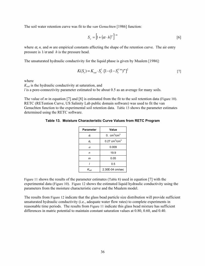
The soil water retention curve was fit to the van Genuchten [1986] function: ( )[ ] mn
e hS−
⋅+= α1 [6]
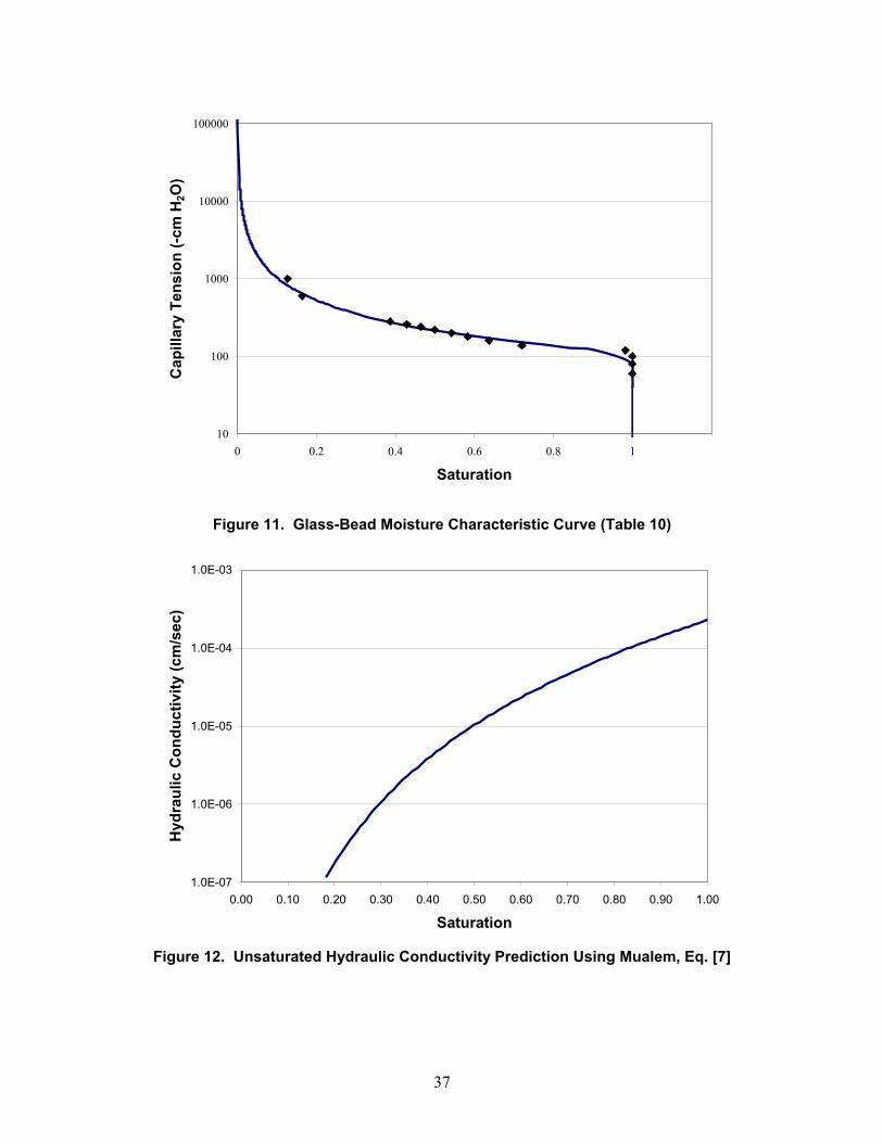
where α, n, and m are empirical constants affecting the shape of the retention curve. The air entry pressure is 1/α and h is the pressure head. The unsaturated hydraulic conductivity for the liquid phase is given by Mualem [1986]: 2/1 ])1(1[)( mm
elesate SSKSK −−⋅⋅= [7]
where Ksat is the hydraulic conductivity at saturation, and l is a pore-connectivity parameter estimated to be about 0.5 as an average for many soils. The value of m in equation [7] and [8] is estimated from the fit to the soil retention data (Figure 10). RETC (RETention Curve, US Salinity Lab public domain software) was used to fit the van Genuchten function to the experimental soil retention data. Table 13 shows the parameter estimates determined using the RETC software.
Table 13. Moisture Characteristic Curve Values from RETC Program
Parameter Value
θr 0. cm3/cm3
θs 0.27 cm3/cm3
α 0.009
n 19.9
m 0.05
l 0.5
Ksat 2.30E-04 cm/sec
Figure 11 shows the results of the parameter estimates (Table 8) used in equation [7] with the experimental data (Figure 10). Figure 12 shows the estimated liquid hydraulic conductivity using the parameters from the moisture characteristic curve and the Mualem model. The results from Figure 12 indicate that the glass bead particle size distribution will provide sufficient unsaturated hydraulic conductivity (i.e., adequate water flow rates) to complete experiments in reasonable time periods. The results from Figure 11 indicate this glass bead mixture has sufficient differences in matric potential to maintain constant saturation values at 0.80, 0.60, and 0.40.
37
10
100
1000
10000
100000
0 0.2 0.4 0.6 0.8 1 1.2
Saturation
Cap
illar
y Te
nsio
n (-c
m H
2O)
Figure 11. Glass-Bead Moisture Characteristic Curve (Table 10)
1.0E-07
1.0E-06
1.0E-05
1.0E-04
1.0E-03
0.00 0.10 0.20 0.30 0.40 0.50 0.60 0.70 0.80 0.90 1.00
Saturation
Hyd
raul
ic C
ondu
ctiv
ity (c
m/s
ec)
Figure 12. Unsaturated Hydraulic Conductivity Prediction Using Mualem, Eq. [7]
38
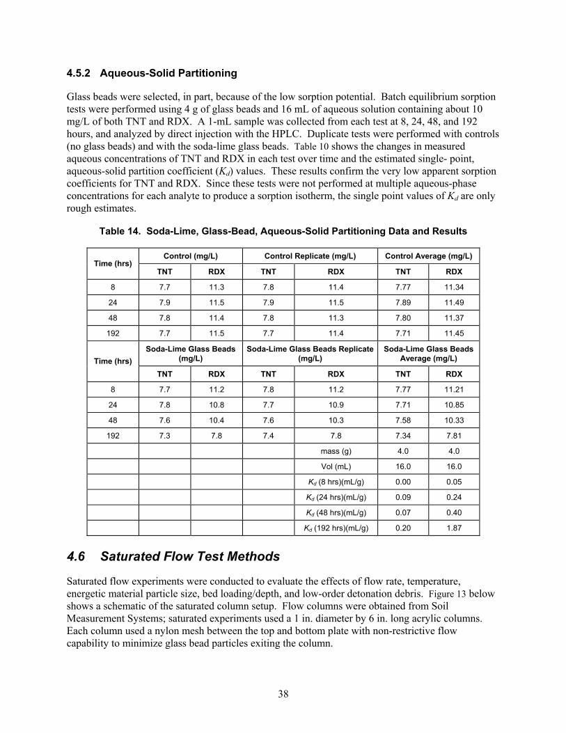
4.5.2 Aqueous-Solid Partitioning
Glass beads were selected, in part, because of the low sorption potential. Batch equilibrium sorption tests were performed using 4 g of glass beads and 16 mL of aqueous solution containing about 10 mg/L of both TNT and RDX. A 1-mL sample was collected from each test at 8, 24, 48, and 192 hours, and analyzed by direct injection with the HPLC. Duplicate tests were performed with controls (no glass beads) and with the soda-lime glass beads. Table 10 shows the changes in measured aqueous concentrations of TNT and RDX in each test over time and the estimated single- point, aqueous-solid partition coefficient (Kd) values. These results confirm the very low apparent sorption coefficients for TNT and RDX. Since these tests were not performed at multiple aqueous-phase concentrations for each analyte to produce a sorption isotherm, the single point values of Kd are only rough estimates.
Table 14. Soda-Lime, Glass-Bead, Aqueous-Solid Partitioning Data and Results
Control (mg/L) Control Replicate (mg/L) Control Average (mg/L) Time (hrs)
TNT RDX TNT RDX TNT RDX
8 7.7 11.3 7.8 11.4 7.77 11.34
24 7.9 11.5 7.9 11.5 7.89 11.49
48 7.8 11.4 7.8 11.3 7.80 11.37
192 7.7 11.5 7.7 11.4 7.71 11.45
Soda-Lime Glass Beads(mg/L)
Soda-Lime Glass Beads Replicate (mg/L)
Soda-Lime Glass Beads Average (mg/L) Time (hrs)
TNT RDX TNT RDX TNT RDX
8 7.7 11.2 7.8 11.2 7.77 11.21
24 7.8 10.8 7.7 10.9 7.71 10.85
48 7.6 10.4 7.6 10.3 7.58 10.33
192 7.3 7.8 7.4 7.8 7.34 7.81
mass (g) 4.0 4.0
Vol (mL) 16.0 16.0
Kd (8 hrs)(mL/g) 0.00 0.05
Kd (24 hrs)(mL/g) 0.09 0.24
Kd (48 hrs)(mL/g) 0.07 0.40
Kd (192 hrs)(mL/g) 0.20 1.87
4.6 Saturated Flow Test Methods
Saturated flow experiments were conducted to evaluate the effects of flow rate, temperature, energetic material particle size, bed loading/depth, and low-order detonation debris. Figure 13 below shows a schematic of the saturated column setup. Flow columns were obtained from Soil Measurement Systems; saturated experiments used a 1 in. diameter by 6 in. long acrylic columns. Each column used a nylon mesh between the top and bottom plate with non-restrictive flow capability to minimize glass bead particles exiting the column.
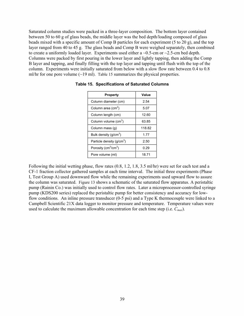
39
Saturated column studies were packed in a three-layer composition. The bottom layer contained between 50 to 60 g of glass beads, the middle layer was the bed depth/loading composed of glass beads mixed with a specific amount of Comp B particles for each experiment (5 to 20 g), and the top layer ranged from 40 to 45 g. The glass beads and Comp B were weighed separately, then combined to create a uniformly loaded layer. Experiments used either a ~0.5-cm or ~2.5-cm bed depth. Columns were packed by first pouring in the lower layer and lightly tapping, then adding the Comp B layer and tapping, and finally filling with the top layer and tapping until flush with the top of the column. Experiments were initially saturated from below with a slow flow rate between 0.4 to 0.8 ml/hr for one pore volume (~19 ml). Table 15 summarizes the physical properties.
Table 15. Specifications of Saturated Columns
Property Value
Column diameter (cm) 2.54
Column area (cm2) 5.07
Column length (cm) 12.60
Column volume (cm3) 63.85
Column mass (g) 118.82
Bulk density (g/cm3) 1.77
Particle density (g/cm3) 2.50
Porosity (cm3/cm3) 0.29
Pore volume (ml) 18.71
Following the initial wetting phase, flow rates (0.8, 1.2, 1.8, 3.5 ml/hr) were set for each test and a CF-1 fraction collector gathered samples at each time interval. The initial three experiments (Phase I, Test Group A) used downward flow while the remaining experiments used upward flow to assure the column was saturated. Figure 13 shows a schematic of the saturated flow apparatus. A peristaltic pump (Rainin Co.) was initially used to control flow rates. Later a microprocessor-controlled syringe pump (KDS200 series) replaced the peristaltic pump for better consistency and accuracy for low-flow conditions. An inline pressure transducer (0-5 psi) and a Type K thermocouple were linked to a Campbell Scientific 21X data logger to monitor pressure and temperature. Temperature values were used to calculate the maximum allowable concentration for each time step (i.e. Cmax).
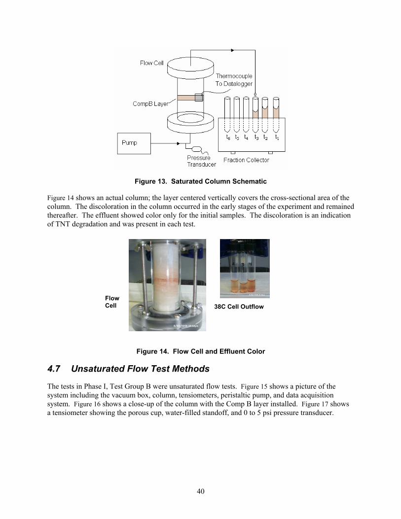
40
Figure 13. Saturated Column Schematic
Figure 14 shows an actual column; the layer centered vertically covers the cross-sectional area of the column. The discoloration in the column occurred in the early stages of the experiment and remained thereafter. The effluent showed color only for the initial samples. The discoloration is an indication of TNT degradation and was present in each test.
Figure 14. Flow Cell and Effluent Color
4.7 Unsaturated Flow Test Methods
The tests in Phase I, Test Group B were unsaturated flow tests. Figure 15 shows a picture of the system including the vacuum box, column, tensiometers, peristaltic pump, and data acquisition system. Figure 16 shows a close-up of the column with the Comp B layer installed. Figure 17 shows a tensiometer showing the porous cup, water-filled standoff, and 0 to 5 psi pressure transducer.
Flow Cell 38C Cell Outflow
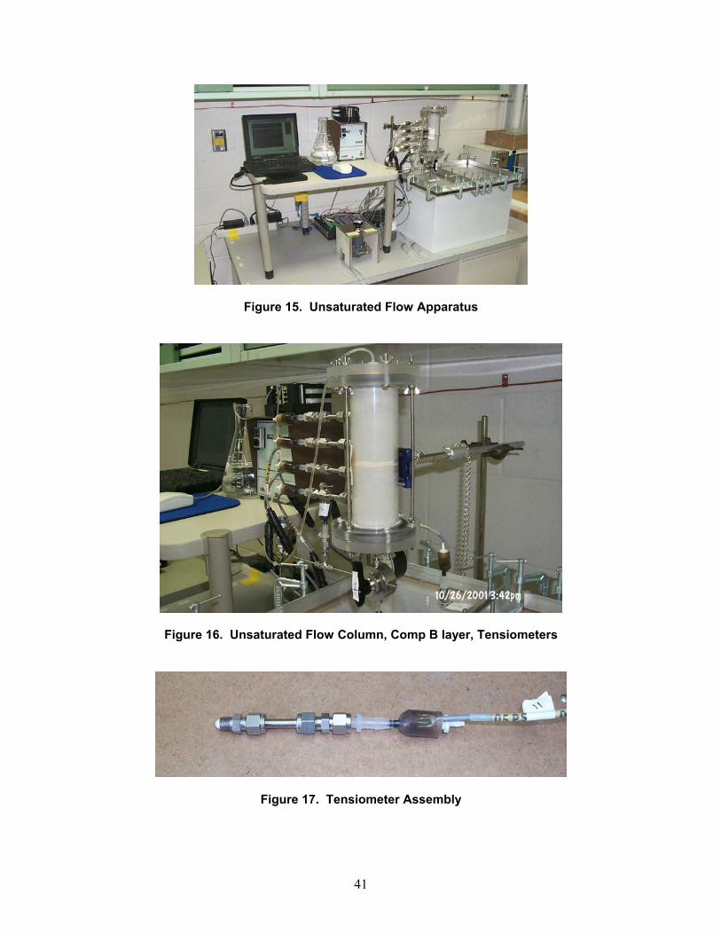
41
Figure 15. Unsaturated Flow Apparatus
Figure 16. Unsaturated Flow Column, Comp B layer, Tensiometers
Figure 17. Tensiometer Assembly
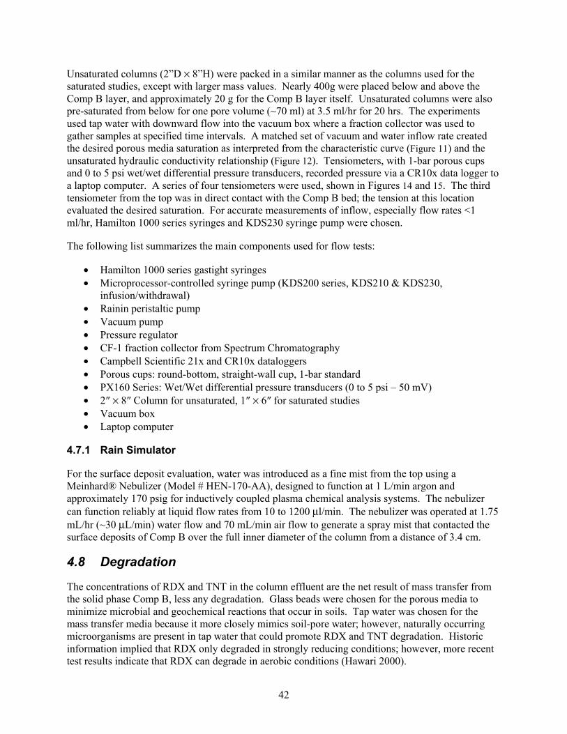
42
Unsaturated columns (2”D × 8”H) were packed in a similar manner as the columns used for the saturated studies, except with larger mass values. Nearly 400g were placed below and above the Comp B layer, and approximately 20 g for the Comp B layer itself. Unsaturated columns were also pre-saturated from below for one pore volume (~70 ml) at 3.5 ml/hr for 20 hrs. The experiments used tap water with downward flow into the vacuum box where a fraction collector was used to gather samples at specified time intervals. A matched set of vacuum and water inflow rate created the desired porous media saturation as interpreted from the characteristic curve (Figure 11) and the unsaturated hydraulic conductivity relationship (Figure 12). Tensiometers, with 1-bar porous cups and 0 to 5 psi wet/wet differential pressure transducers, recorded pressure via a CR10x data logger to a laptop computer. A series of four tensiometers were used, shown in Figures 14 and 15. The third tensiometer from the top was in direct contact with the Comp B bed; the tension at this location evaluated the desired saturation. For accurate measurements of inflow, especially flow rates <1 ml/hr, Hamilton 1000 series syringes and KDS230 syringe pump were chosen. The following list summarizes the main components used for flow tests:
• Hamilton 1000 series gastight syringes • Microprocessor-controlled syringe pump (KDS200 series, KDS210 & KDS230,
infusion/withdrawal) • Rainin peristaltic pump • Vacuum pump • Pressure regulator • CF-1 fraction collector from Spectrum Chromatography • Campbell Scientific 21x and CR10x dataloggers • Porous cups: round-bottom, straight-wall cup, 1-bar standard • PX160 Series: Wet/Wet differential pressure transducers (0 to 5 psi – 50 mV) • 2″ × 8″ Column for unsaturated, 1″ × 6″ for saturated studies • Vacuum box • Laptop computer
4.7.1 Rain Simulator
For the surface deposit evaluation, water was introduced as a fine mist from the top using a Meinhard® Nebulizer (Model # HEN-170-AA), designed to function at 1 L/min argon and approximately 170 psig for inductively coupled plasma chemical analysis systems. The nebulizer can function reliably at liquid flow rates from 10 to 1200 μl/min. The nebulizer was operated at 1.75 mL/hr (~30 μL/min) water flow and 70 mL/min air flow to generate a spray mist that contacted the surface deposits of Comp B over the full inner diameter of the column from a distance of 3.4 cm. 4.8 Degradation
The concentrations of RDX and TNT in the column effluent are the net result of mass transfer from the solid phase Comp B, less any degradation. Glass beads were chosen for the porous media to minimize microbial and geochemical reactions that occur in soils. Tap water was chosen for the mass transfer media because it more closely mimics soil-pore water; however, naturally occurring microorganisms are present in tap water that could promote RDX and TNT degradation. Historic information implied that RDX only degraded in strongly reducing conditions; however, more recent test results indicate that RDX can degrade in aerobic conditions (Hawari 2000).
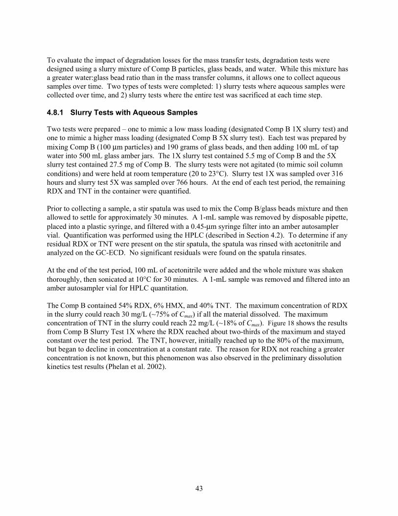
43
To evaluate the impact of degradation losses for the mass transfer tests, degradation tests were designed using a slurry mixture of Comp B particles, glass beads, and water. While this mixture has a greater water:glass bead ratio than in the mass transfer columns, it allows one to collect aqueous samples over time. Two types of tests were completed: 1) slurry tests where aqueous samples were collected over time, and 2) slurry tests where the entire test was sacrificed at each time step. 4.8.1 Slurry Tests with Aqueous Samples
Two tests were prepared – one to mimic a low mass loading (designated Comp B 1X slurry test) and one to mimic a higher mass loading (designated Comp B 5X slurry test). Each test was prepared by mixing Comp B (100 μm particles) and 190 grams of glass beads, and then adding 100 mL of tap water into 500 mL glass amber jars. The 1X slurry test contained 5.5 mg of Comp B and the 5X slurry test contained 27.5 mg of Comp B. The slurry tests were not agitated (to mimic soil column conditions) and were held at room temperature (20 to 23°C). Slurry test 1X was sampled over 316 hours and slurry test 5X was sampled over 766 hours. At the end of each test period, the remaining RDX and TNT in the container were quantified. Prior to collecting a sample, a stir spatula was used to mix the Comp B/glass beads mixture and then allowed to settle for approximately 30 minutes. A 1-mL sample was removed by disposable pipette, placed into a plastic syringe, and filtered with a 0.45-μm syringe filter into an amber autosampler vial. Quantification was performed using the HPLC (described in Section 4.2). To determine if any residual RDX or TNT were present on the stir spatula, the spatula was rinsed with acetonitrile and analyzed on the GC-ECD. No significant residuals were found on the spatula rinsates. At the end of the test period, 100 mL of acetonitrile were added and the whole mixture was shaken thoroughly, then sonicated at 10°C for 30 minutes. A 1-mL sample was removed and filtered into an amber autosampler vial for HPLC quantitation. The Comp B contained 54% RDX, 6% HMX, and 40% TNT. The maximum concentration of RDX in the slurry could reach 30 mg/L (~75% of Cmax) if all the material dissolved. The maximum concentration of TNT in the slurry could reach 22 mg/L (~18% of Cmax). Figure 18 shows the results from Comp B Slurry Test 1X where the RDX reached about two-thirds of the maximum and stayed constant over the test period. The TNT, however, initially reached up to the 80% of the maximum, but began to decline in concentration at a constant rate. The reason for RDX not reaching a greater concentration is not known, but this phenomenon was also observed in the preliminary dissolution kinetics test results (Phelan et al. 2002).
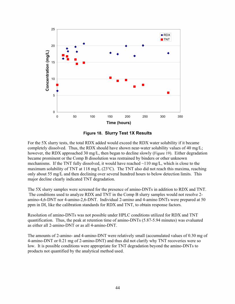
44
0
5
10
15
20
25
0 50 100 150 200 250 300 350
Time (hours)
Con
cent
ratio
n (m
g/L)
RDXTNT
Figure 18. Slurry Test 1X Results
For the 5X slurry tests, the total RDX added would exceed the RDX water solubility if it became completely dissolved. Thus, the RDX should have shown near-water solubility values of 40 mg/L; however, the RDX approached 30 mg/L, then began to decline slowly (Figure 19). Either degradation became prominent or the Comp B dissolution was restrained by binders or other unknown mechanisms. If the TNT fully dissolved, it would have reached ~110 mg/L, which is close to the maximum solubility of TNT at 118 mg/L (23°C). The TNT also did not reach this maxima, reaching only about 55 mg/L and then declining over several hundred hours to below detection limits. This major decline clearly indicated TNT degradation. The 5X slurry samples were screened for the presence of amino-DNTs in addition to RDX and TNT. The conditions used to analyze RDX and TNT in the Comp B slurry samples would not resolve 2-amino-4,6-DNT nor 4-amino-2,6-DNT. Individual 2-amino and 4-amino DNTs were prepared at 50 ppm in DI, like the calibration standards for RDX and TNT, to obtain response factors. Resolution of amino-DNTs was not possible under HPLC conditions utilized for RDX and TNT quantification. Thus, the peak at retention time of amino-DNTs (5.87-5.94 minutes) was evaluated as either all 2-amino-DNT or as all 4-amino-DNT. The amounts of 2-amino- and 4-amino-DNT were relatively small (accumulated values of 0.30 mg of 4-amino-DNT or 0.21 mg of 2-amino-DNT) and thus did not clarify why TNT recoveries were so low. It is possible conditions were appropriate for TNT degradation beyond the amino-DNTs to products not quantified by the analytical method used.
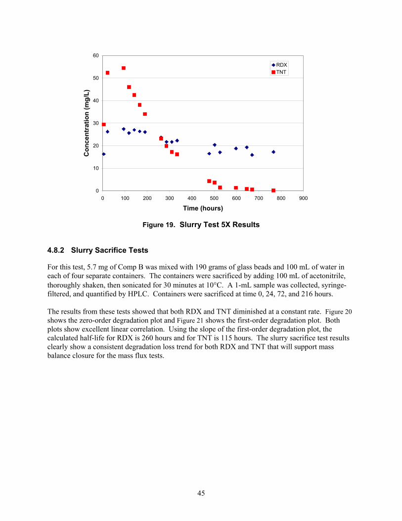
45
0
10
20
30
40
50
60
0 100 200 300 400 500 600 700 800 900
Time (hours)
Con
cent
ratio
n (m
g/L)
RDXTNT
Figure 19. Slurry Test 5X Results
4.8.2 Slurry Sacrifice Tests
For this test, 5.7 mg of Comp B was mixed with 190 grams of glass beads and 100 mL of water in each of four separate containers. The containers were sacrificed by adding 100 mL of acetonitrile, thoroughly shaken, then sonicated for 30 minutes at 10°C. A 1-mL sample was collected, syringe-filtered, and quantified by HPLC. Containers were sacrificed at time 0, 24, 72, and 216 hours. The results from these tests showed that both RDX and TNT diminished at a constant rate. Figure 20 shows the zero-order degradation plot and Figure 21 shows the first-order degradation plot. Both plots show excellent linear correlation. Using the slope of the first-order degradation plot, the calculated half-life for RDX is 260 hours and for TNT is 115 hours. The slurry sacrifice test results clearly show a consistent degradation loss trend for both RDX and TNT that will support mass balance closure for the mass flux tests.
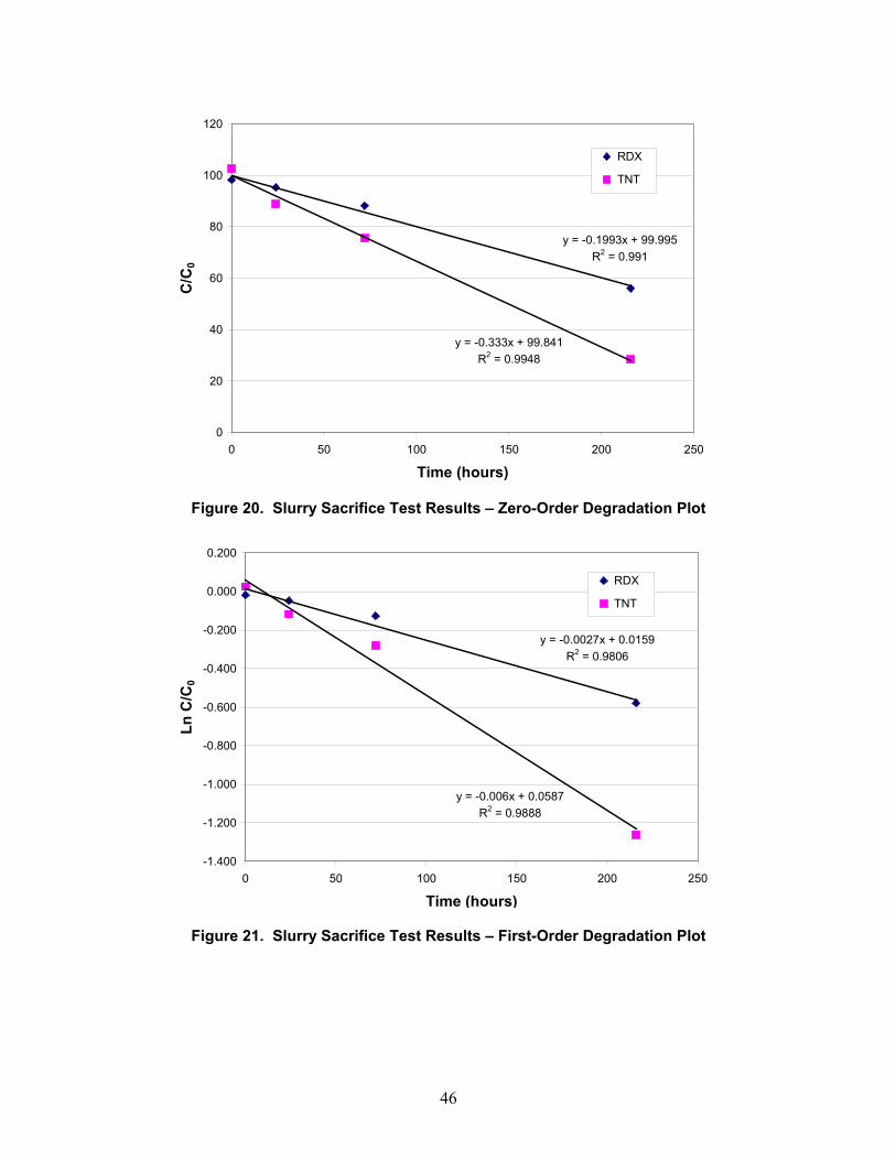
46
y = -0.1993x + 99.995R2 = 0.991
y = -0.333x + 99.841R2 = 0.9948
0
20
40
60
80
100
120
0 50 100 150 200 250
Time (hours)
C/C
0
RDX
TNT
Figure 20. Slurry Sacrifice Test Results – Zero-Order Degradation Plot
y = -0.0027x + 0.0159R2 = 0.9806
y = -0.006x + 0.0587R2 = 0.9888
-1.400
-1.200
-1.000
-0.800
-0.600
-0.400
-0.200
0.000
0.200
0 50 100 150 200 250
Time (hours)
Ln C
/C0
RDX
TNT
Figure 21. Slurry Sacrifice Test Results – First-Order Degradation Plot
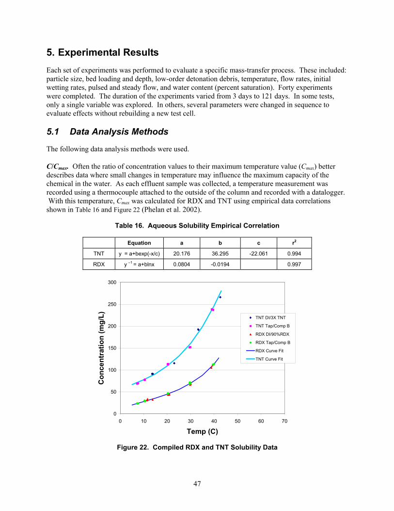
47
5. Experimental Results Each set of experiments was performed to evaluate a specific mass-transfer process. These included: particle size, bed loading and depth, low-order detonation debris, temperature, flow rates, initial wetting rates, pulsed and steady flow, and water content (percent saturation). Forty experiments were completed. The duration of the experiments varied from 3 days to 121 days. In some tests, only a single variable was explored. In others, several parameters were changed in sequence to evaluate effects without rebuilding a new test cell. 5.1 Data Analysis Methods
The following data analysis methods were used. C/Cmax. Often the ratio of concentration values to their maximum temperature value (Cmax) better describes data where small changes in temperature may influence the maximum capacity of the chemical in the water. As each effluent sample was collected, a temperature measurement was recorded using a thermocouple attached to the outside of the column and recorded with a datalogger. With this temperature, Cmax was calculated for RDX and TNT using empirical data correlations shown in Table 16 and Figure 22 (Phelan et al. 2002).
Table 16. Aqueous Solubility Empirical Correlation
Equation a b c r2
TNT y = a+bexp(-x/c) 20.176 36.295 -22.061 0.994
RDX y –1 = a+blnx 0.0804 -0.0194 0.997
0
50
100
150
200
250
300
0 10 20 30 40 50 60 70
Temp (C)
Con
cent
ratio
n (m
g/L) TNT DI/3X TNT
TNT Tap/Comp B
RDX DI/90%RDX
RDX Tap/Comp B
RDX Curve Fit
TNT Curve Fit
Figure 22. Compiled RDX and TNT Solubility Data
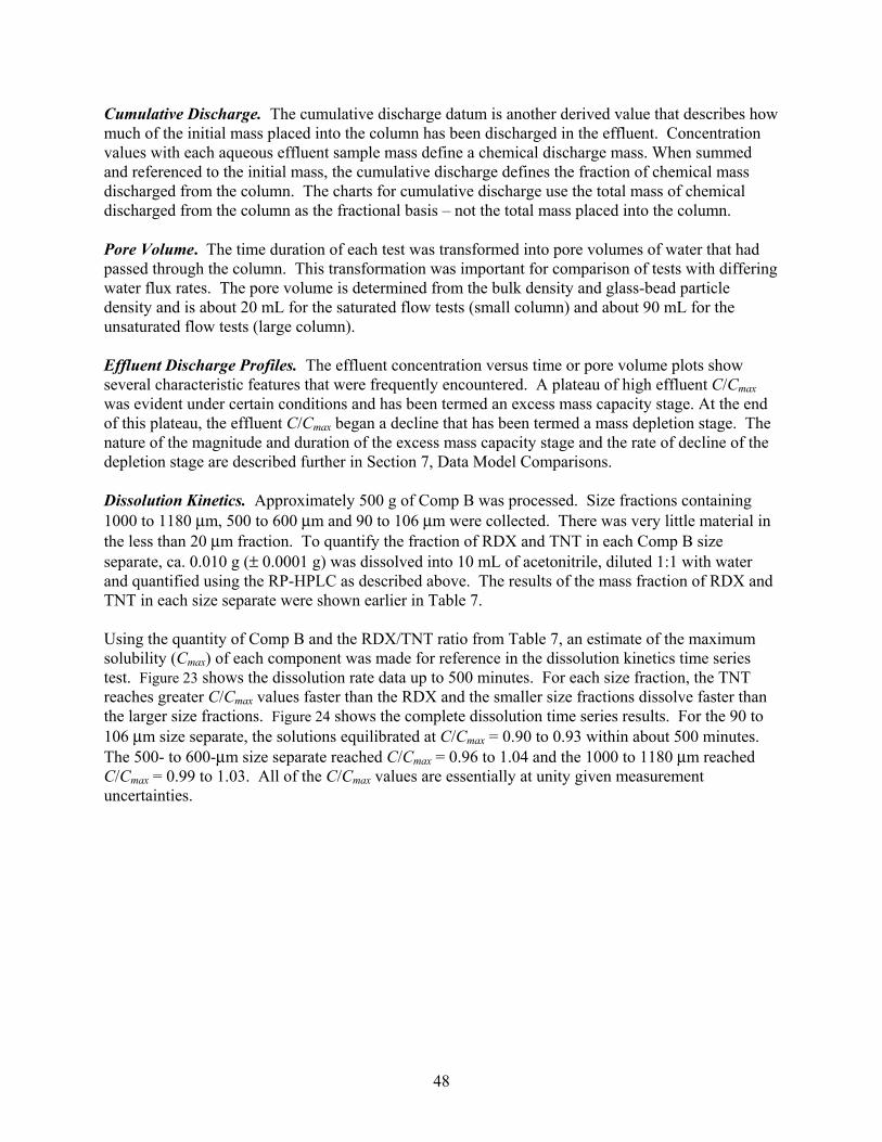
48
Cumulative Discharge. The cumulative discharge datum is another derived value that describes how much of the initial mass placed into the column has been discharged in the effluent. Concentration values with each aqueous effluent sample mass define a chemical discharge mass. When summed and referenced to the initial mass, the cumulative discharge defines the fraction of chemical mass discharged from the column. The charts for cumulative discharge use the total mass of chemical discharged from the column as the fractional basis – not the total mass placed into the column. Pore Volume. The time duration of each test was transformed into pore volumes of water that had passed through the column. This transformation was important for comparison of tests with differing water flux rates. The pore volume is determined from the bulk density and glass-bead particle density and is about 20 mL for the saturated flow tests (small column) and about 90 mL for the unsaturated flow tests (large column). Effluent Discharge Profiles. The effluent concentration versus time or pore volume plots show several characteristic features that were frequently encountered. A plateau of high effluent C/Cmax was evident under certain conditions and has been termed an excess mass capacity stage. At the end of this plateau, the effluent C/Cmax began a decline that has been termed a mass depletion stage. The nature of the magnitude and duration of the excess mass capacity stage and the rate of decline of the depletion stage are described further in Section 7, Data Model Comparisons. Dissolution Kinetics. Approximately 500 g of Comp B was processed. Size fractions containing 1000 to 1180 μm, 500 to 600 μm and 90 to 106 μm were collected. There was very little material in the less than 20 μm fraction. To quantify the fraction of RDX and TNT in each Comp B size separate, ca. 0.010 g (± 0.0001 g) was dissolved into 10 mL of acetonitrile, diluted 1:1 with water and quantified using the RP-HPLC as described above. The results of the mass fraction of RDX and TNT in each size separate were shown earlier in Table 7. Using the quantity of Comp B and the RDX/TNT ratio from Table 7, an estimate of the maximum solubility (Cmax) of each component was made for reference in the dissolution kinetics time series test. Figure 23 shows the dissolution rate data up to 500 minutes. For each size fraction, the TNT reaches greater C/Cmax values faster than the RDX and the smaller size fractions dissolve faster than the larger size fractions. Figure 24 shows the complete dissolution time series results. For the 90 to 106 μm size separate, the solutions equilibrated at C/Cmax = 0.90 to 0.93 within about 500 minutes. The 500- to 600-μm size separate reached C/Cmax = 0.96 to 1.04 and the 1000 to 1180 μm reached C/Cmax = 0.99 to 1.03. All of the C/Cmax values are essentially at unity given measurement uncertainties.
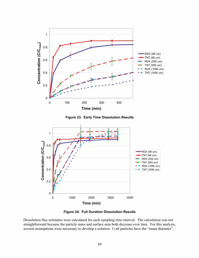
49
0
0.2
0.4
0.6
0.8
1
0 100 200 300 400
Time (min)
Con
cent
ratio
n (C
/Cm
ax)
RDX (98 um)TNT (98 um)RDX (550 um)TNT (550 um)RDX (1090 um)TNT (1090 um)
Figure 23. Early Time Dissolution Results
0
0.2
0.4
0.6
0.8
1
0 1000 2000 3000 4000
Time (min)
Con
cent
ratio
n (C
/Cm
ax)
RDX (98 um)TNT (98 um)RDX (550 um)TNT (550 um)RDX (1090 um)TNT (1090 um)
Figure 24. Full Duration Dissolution Results
Dissolution flux estimates were calculated for each sampling time interval. The calculation was not straightforward because the particle mass and surface area both decrease over time. For this analysis, several assumptions were necessary to develop a solution: 1) all particles have the “mean diameter”,
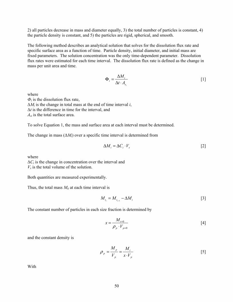
50
2) all particles decrease in mass and diameter equally, 3) the total number of particles is constant, 4) the particle density is constant, and 5) the particles are rigid, spherical, and smooth. The following method describes an analytical solution that solves for the dissolution flux rate and specific surface area as a function of time. Particle density, initial diameter, and initial mass are fixed parameters. The solution concentration was the only time-dependent parameter. Dissolution flux rates were estimated for each time interval. The dissolution flux rate is defined as the change in mass per unit area and time.
is
ii At
M⋅Δ
Δ=Φ [1]
where Фi is the dissolution flux rate, ΔMi is the change in total mass at the end of time interval i, Δt is the difference in time for the interval, and Asi is the total surface area. To solve Equation 1, the mass and surface area at each interval must be determined. The change in mass (ΔMi) over a specific time interval is determined from sii VCM ⋅Δ=Δ [2]
where ΔCi is the change in concentration over the interval and Vs is the total volume of the solution. Both quantities are measured experimentally. Thus, the total mass Mti at each time interval is itt MMM
iiΔ−=
−1 [3]
The constant number of particles in each size fraction is determined by
0
0
=
=
⋅=
pp
t
VMx
ρ [4]
and the constant density is
p
t
p
pp Vx
MVM
⋅==ρ [5]
With
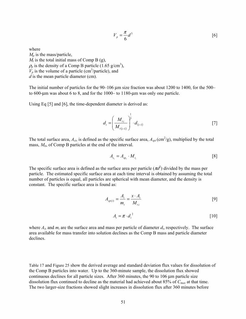
51
3
6dVp
π= [6]
where Mp is the mass/particle, Mt is the total initial mass of Comp B (g), ρp is the density of a Comp B particle (1.65 g/cm3), Vp is the volume of a particle (cm3/particle), and d is the mean particle diameter (cm). The initial number of particles for the 90–106 μm size fraction was about 1200 to 1400, for the 500– to 600-μm was about 6 to 8, and for the 1000– to 1180-μm was only one particle. Using Eq [5] and [6], the time-dependent diameter is derived as:
( )
( )1
31
1−
−
⋅⎟⎟⎠
⎞⎜⎜⎝
⎛= i
it
iti d
MM
d [7]
The total surface area, Asi, is defined as the specific surface area, Aspi (cm2/g), multiplied by the total mass, Mti, of Comp B particles at the end of the interval.
iii tsps MAA ⋅= [8]
The specific surface area is defined as the surface area per particle (πd2) divided by the mass per particle. The estimated specific surface area at each time interval is obtained by assuming the total number of particles is equal, all particles are spherical with mean diameter, and the density is constant. The specific surface area is found as:
it
i
i
iisp M
AxmA
A⋅
==)( [9]
2ii dA ⋅= π [10]
where Ai, and mi are the surface area and mass per particle of diameter di, respectively. The surface area available for mass transfer into solution declines as the Comp B mass and particle diameter declines. Table 17 and Figure 25 show the derived average and standard deviation flux values for dissolution of the Comp B particles into water. Up to the 360-minute sample, the dissolution flux showed continuous declines for all particle sizes. After 360 minutes, the 90 to 106 μm particle size dissolution flux continued to decline as the material had achieved about 85% of Cmax at that time. The two larger-size fractions showed slight increases in dissolution flux after 360 minutes before
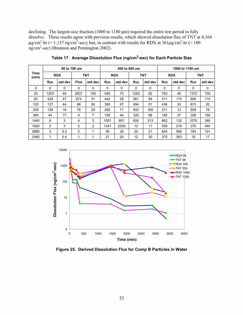
52
declining. The largest-size fraction (1000 to 1180 μm) required the entire test period to fully dissolve. These results agree with previous results, which showed dissolution flux of TNT at 4,164 μg/cm2-hr (= 1,157 ng/cm2-sec); but, in contrast with results for RDX at 361μg/cm2-hr (= 100 ng/cm2-sec) (Brannon and Pennington 2002).
Table 17. Average Dissolution Flux (ng/cm2-sec) for Each Particle Size
90 to 106 um 500 to 600 um 1000 to 1180 um
RDX TNT RDX TNT RDX TNT Time (min)
flux std dev Flux std dev flux std dev flux std dev flux std dev flux std dev
0 0 0 0 0 0 0 0 0 0 0 0 0 20 1203 40 2837 150 540 75 1263 82 763 46 1372 150 60 428 47 674 31 442 28 981 88 511 115 908 110 120 127 44 88 50 360 67 694 51 436 33 673 20 240 139 16 79 29 265 71 503 165 311 13 559 76 360 44 17 4 7 156 44 320 88 165 37 208 180
1440 8 3 4 3 1051 601 826 213 862 132 1070 360 1920 3 3 2 2 1341 2293 12 11 530 218 370 440 2880 3 0.3 2 1 36 26 20 21 824 566 184 101 3360 1 0.4 1 1 21 24 12 20 375 363 19 17
0
1
10
100
1000
10000
0 500 1000 1500 2000 2500 3000 3500 4000
Time (min)
Dis
solu
tion
Flux
(ng/
cm2 -s
ec)
RDX 98TNT 98RDX 550TNT 550RDX 1090TNT 1090
Figure 25. Derived Dissolution Flux for Comp B Particles in Water
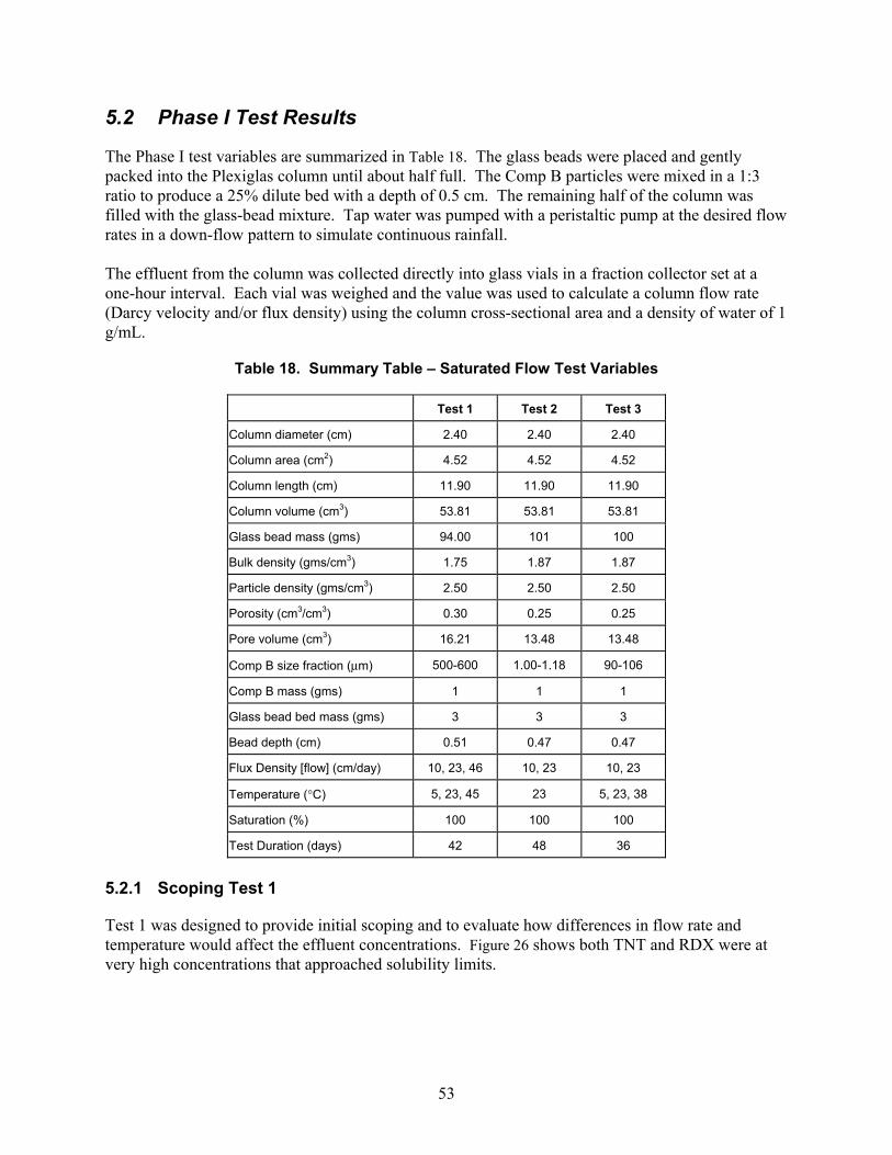
53
5.2 Phase I Test Results
The Phase I test variables are summarized in Table 18. The glass beads were placed and gently packed into the Plexiglas column until about half full. The Comp B particles were mixed in a 1:3 ratio to produce a 25% dilute bed with a depth of 0.5 cm. The remaining half of the column was filled with the glass-bead mixture. Tap water was pumped with a peristaltic pump at the desired flow rates in a down-flow pattern to simulate continuous rainfall. The effluent from the column was collected directly into glass vials in a fraction collector set at a one-hour interval. Each vial was weighed and the value was used to calculate a column flow rate (Darcy velocity and/or flux density) using the column cross-sectional area and a density of water of 1 g/mL.
Table 18. Summary Table – Saturated Flow Test Variables
Test 1 Test 2 Test 3
Column diameter (cm) 2.40 2.40 2.40
Column area (cm2) 4.52 4.52 4.52
Column length (cm) 11.90 11.90 11.90
Column volume (cm3) 53.81 53.81 53.81
Glass bead mass (gms) 94.00 101 100
Bulk density (gms/cm3) 1.75 1.87 1.87
Particle density (gms/cm3) 2.50 2.50 2.50
Porosity (cm3/cm3) 0.30 0.25 0.25
Pore volume (cm3) 16.21 13.48 13.48
Comp B size fraction (μm) 500-600 1.00-1.18 90-106
Comp B mass (gms) 1 1 1
Glass bead bed mass (gms) 3 3 3
Bead depth (cm) 0.51 0.47 0.47
Flux Density [flow] (cm/day) 10, 23, 46 10, 23 10, 23
Temperature (°C) 5, 23, 45 23 5, 23, 38
Saturation (%) 100 100 100
Test Duration (days) 42 48 36
5.2.1 Scoping Test 1
Test 1 was designed to provide initial scoping and to evaluate how differences in flow rate and temperature would affect the effluent concentrations. Figure 26 shows both TNT and RDX were at very high concentrations that approached solubility limits.
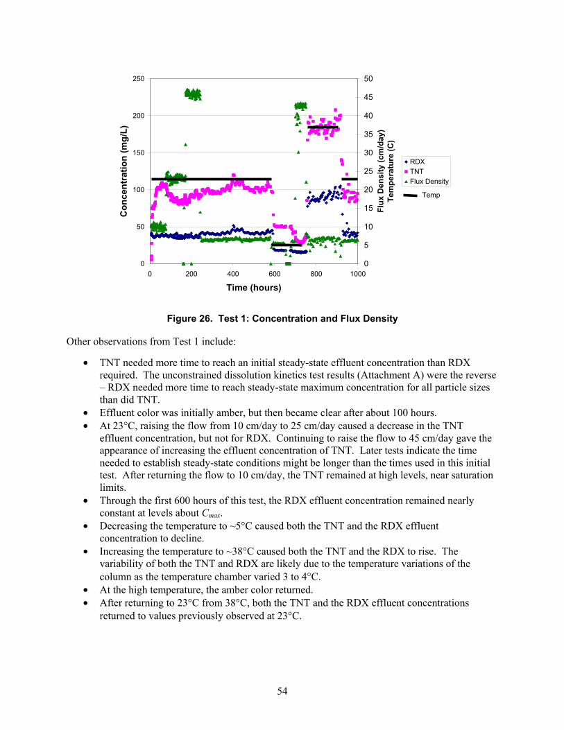
54
0
50
100
150
200
250
0 200 400 600 800 1000
Time (hours)
Con
cent
ratio
n (m
g/L)
0
5
10
15
20
25
30
35
40
45
50
Flux
Den
sity
(cm
/day
)Te
mpe
ratu
re (C
)
RDXTNTFlux Density
Temp
Figure 26. Test 1: Concentration and Flux Density
Other observations from Test 1 include:
• TNT needed more time to reach an initial steady-state effluent concentration than RDX required. The unconstrained dissolution kinetics test results (Attachment A) were the reverse – RDX needed more time to reach steady-state maximum concentration for all particle sizes than did TNT.
• Effluent color was initially amber, but then became clear after about 100 hours. • At 23°C, raising the flow from 10 cm/day to 25 cm/day caused a decrease in the TNT
effluent concentration, but not for RDX. Continuing to raise the flow to 45 cm/day gave the appearance of increasing the effluent concentration of TNT. Later tests indicate the time needed to establish steady-state conditions might be longer than the times used in this initial test. After returning the flow to 10 cm/day, the TNT remained at high levels, near saturation limits.
• Through the first 600 hours of this test, the RDX effluent concentration remained nearly constant at levels about Cmax.
• Decreasing the temperature to ~5°C caused both the TNT and the RDX effluent concentration to decline.
• Increasing the temperature to ~38°C caused both the TNT and the RDX to rise. The variability of both the TNT and RDX are likely due to the temperature variations of the column as the temperature chamber varied 3 to 4°C.
• At the high temperature, the amber color returned. • After returning to 23°C from 38°C, both the TNT and the RDX effluent concentrations
returned to values previously observed at 23°C.

55
5.2.2 Scoping Test 2
Test 2 used the largest Comp B particles (1000 to 1180 μm). A thermocouple was placed on the column adjacent to the dilute bed of Comp B to monitor the slight variations in temperature after about 200 hours. This test also sought to evaluate the time required to establish steady-state con-ditions. Figure 27 shows the concentration, temperature, and flux density over time. Figure 28 shows the ratio of effluent concentration (C) to the maximum solution concentration (Cmax) at the column temperature with the column flow rate (flux density). Figure 29 shows the cumulative discharge of both TNT and RDX as a percentage of the original mass placed into the column.
0
20
40
60
80
100
120
0 200 400 600 800 1000
Time (hours)
Con
cent
ratio
n (m
g/L)
0
5
10
15
20
25
30
35
40
45
50
Tem
pera
ture
(C)
Flux
Den
sity
(cm
/day
)
RDXTNTTNT CmaxRDX CmaxCell TempFlux Density
Figure 27. Test 2: Concentration, Temperature, and Flux Density
40
50
60
70
80
90
100
0 200 400 600 800 1000
Time (hours)
Efflu
ent C
once
ntra
tion
(C/C
max
)
0
10
20
30
40
50
60
Flux
Den
sity
(cm
/day
)
TNTRDXFlux Density
Figure 28. Test 2: TNT and RDX C/Cmax
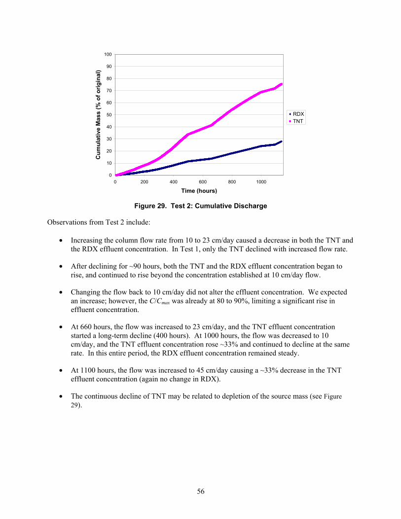
56
0
10
20
30
40
50
60
70
80
90
100
0 200 400 600 800 1000
Time (hours)
Cum
ulat
ive
Mas
s (%
of o
rigin
al)
RDXTNT
Figure 29. Test 2: Cumulative Discharge
Observations from Test 2 include:
• Increasing the column flow rate from 10 to 23 cm/day caused a decrease in both the TNT and the RDX effluent concentration. In Test 1, only the TNT declined with increased flow rate.
• After declining for ~90 hours, both the TNT and the RDX effluent concentration began to rise, and continued to rise beyond the concentration established at 10 cm/day flow.
• Changing the flow back to 10 cm/day did not alter the effluent concentration. We expected an increase; however, the C/Cmax was already at 80 to 90%, limiting a significant rise in effluent concentration.
• At 660 hours, the flow was increased to 23 cm/day, and the TNT effluent concentration started a long-term decline (400 hours). At 1000 hours, the flow was decreased to 10 cm/day, and the TNT effluent concentration rose ~33% and continued to decline at the same rate. In this entire period, the RDX effluent concentration remained steady.
• At 1100 hours, the flow was increased to 45 cm/day causing a ~33% decrease in the TNT effluent concentration (again no change in RDX).
• The continuous decline of TNT may be related to depletion of the source mass (see Figure 29).
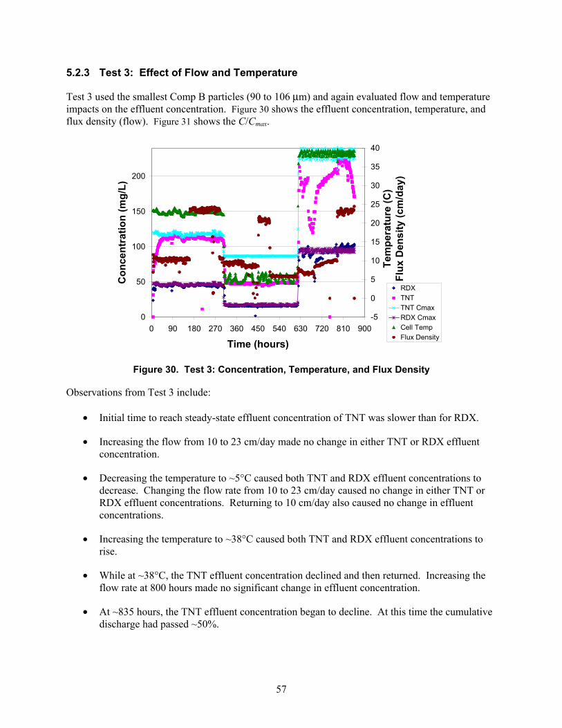
57
5.2.3 Test 3: Effect of Flow and Temperature
Test 3 used the smallest Comp B particles (90 to 106 μm) and again evaluated flow and temperature impacts on the effluent concentration. Figure 30 shows the effluent concentration, temperature, and flux density (flow). Figure 31 shows the C/Cmax.
0
50
100
150
200
0 90 180 270 360 450 540 630 720 810 900
Time (hours)
Con
cent
ratio
n (m
g/L)
-5
0
5
10
15
20
25
30
35
40
Tem
pera
ture
(C)
Flux
Den
sity
(cm
/day
)
RDXTNTTNT CmaxRDX CmaxCell TempFlux Density
Figure 30. Test 3: Concentration, Temperature, and Flux Density
Observations from Test 3 include:
• Initial time to reach steady-state effluent concentration of TNT was slower than for RDX.
• Increasing the flow from 10 to 23 cm/day made no change in either TNT or RDX effluent concentration.
• Decreasing the temperature to ~5°C caused both TNT and RDX effluent concentrations to decrease. Changing the flow rate from 10 to 23 cm/day caused no change in either TNT or RDX effluent concentrations. Returning to 10 cm/day also caused no change in effluent concentrations.
• Increasing the temperature to ~38°C caused both TNT and RDX effluent concentrations to rise.
• While at ~38°C, the TNT effluent concentration declined and then returned. Increasing the flow rate at 800 hours made no significant change in effluent concentration.
• At ~835 hours, the TNT effluent concentration began to decline. At this time the cumulative discharge had passed ~50%.
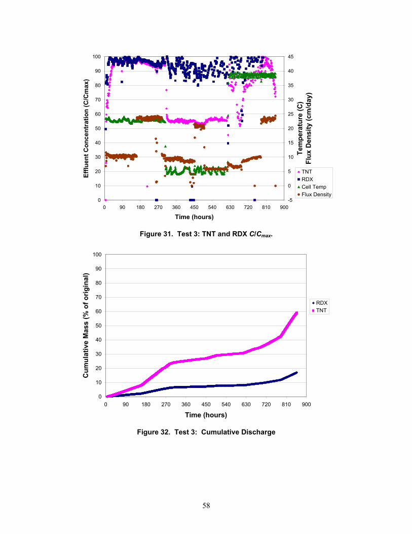
58
0
10
20
30
40
50
60
70
80
90
100
0 90 180 270 360 450 540 630 720 810 900
Time (hours)
Efflu
ent C
once
ntra
tion
(C/C
max
)
-5
0
5
10
15
20
25
30
35
40
45
Tem
pera
ture
(C)
Flux
Den
sity
(cm
/day
)
TNTRDXCell TempFlux Density
Figure 31. Test 3: TNT and RDX C/Cmax.
0
10
20
30
40
50
60
70
80
90
100
0 90 180 270 360 450 540 630 720 810 900
Time (hours)
Cum
ulat
ive
Mas
s (%
of o
rigin
al)
RDXTNT
Figure 32. Test 3: Cumulative Discharge
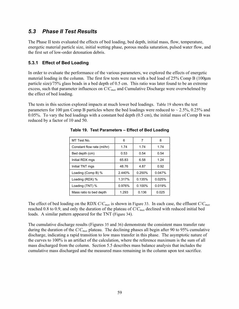
59
5.3 Phase II Test Results
The Phase II tests evaluated the effects of bed loading, bed depth, initial mass, flow, temperature, energetic material particle size, initial wetting phase, porous media saturation, pulsed water flow, and the first set of low-order detonation debris. 5.3.1 Effect of Bed Loading
In order to evaluate the performance of the various parameters, we explored the effects of energetic material loading in the column. The first few tests were run with a bed load of 25% Comp B (100μm particle size)/75% glass beads in a bed depth of 0.5 cm. This ratio was later found to be an extreme excess, such that parameter influences on C/Cmax and Cumulative Discharge were overwhelmed by the effect of bed loading. The tests in this section explored impacts at much lower bed loadings. Table 19 shows the test parameters for 100 μm Comp B particles where the bed loadings were reduced to ~ 2.5%, 0.25% and 0.05%. To vary the bed loadings with a constant bed depth (0.5 cm), the initial mass of Comp B was reduced by a factor of 10 and 50.
Table 19. Test Parameters – Effect of Bed Loading
MT Test No. 6 7 8
Constant flow rate (ml/hr) 1.74 1.74 1.74
Bed depth (cm) 0.53 0.54 0.54
Initial RDX mgs 65.83 6.58 1.24
Initial TNT mgs 48.76 4.87 0.92
Loading (Comp B) % 2.440% 0.250% 0.047%
Loading (RDX) % 1.317% 0.135% 0.025%
Loading (TNT) % 0.976% 0.100% 0.019%
Mass ratio to bed depth 1.293 0.136 0.025
The effect of bed loading on the RDX C/Cmax is shown in Figure 33. In each case, the effluent C/Cmax reached 0.8 to 0.9, and only the duration of the plateau of C/Cmax declined with reduced initial bed loads. A similar pattern appeared for the TNT (Figure 34). The cumulative discharge results (Figures 35 and 36) demonstrate the consistent mass transfer rate during the duration of the C/Cmax plateau. The declining phases all begin after 90 to 95% cumulative discharge, indicating a rapid transition to low mass transfer in this phase. The asymptotic nature of the curves to 100% is an artifact of the calculation, where the reference maximum is the sum of all mass discharged from the column. Section 5.5 describes mass balance analysis that includes the cumulative mass discharged and the measured mass remaining in the column upon test sacrifice.
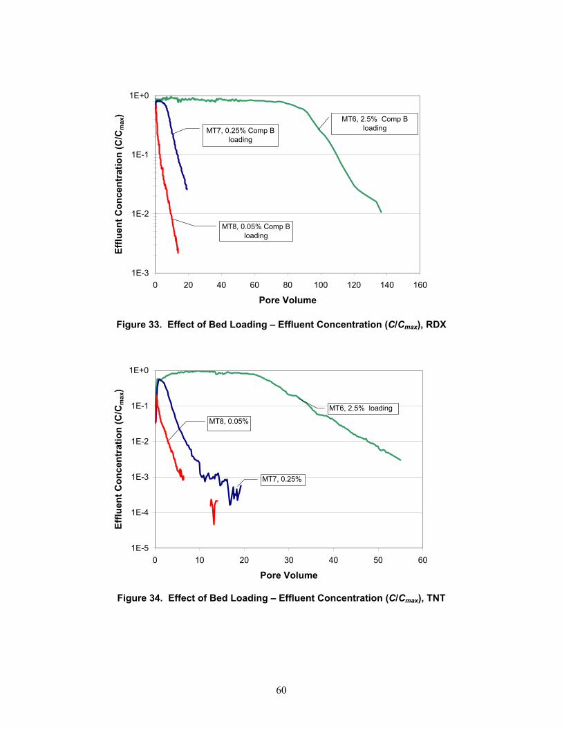
60
1E-3
1E-2
1E-1
1E+0
0 20 40 60 80 100 120 140 160
Pore Volume
Efflu
ent C
once
ntra
tion
(C/C
max
) MT6, 2.5% Comp B loadingMT7, 0.25% Comp B
loading
MT8, 0.05% Comp B loading
Figure 33. Effect of Bed Loading – Effluent Concentration (C/Cmax), RDX
1E-5
1E-4
1E-3
1E-2
1E-1
1E+0
0 10 20 30 40 50 60
Pore Volume
Efflu
ent C
once
ntra
tion
(C/C
max
)
MT6, 2.5% loading
MT7, 0.25%
MT8, 0.05%
Figure 34. Effect of Bed Loading – Effluent Concentration (C/Cmax), TNT
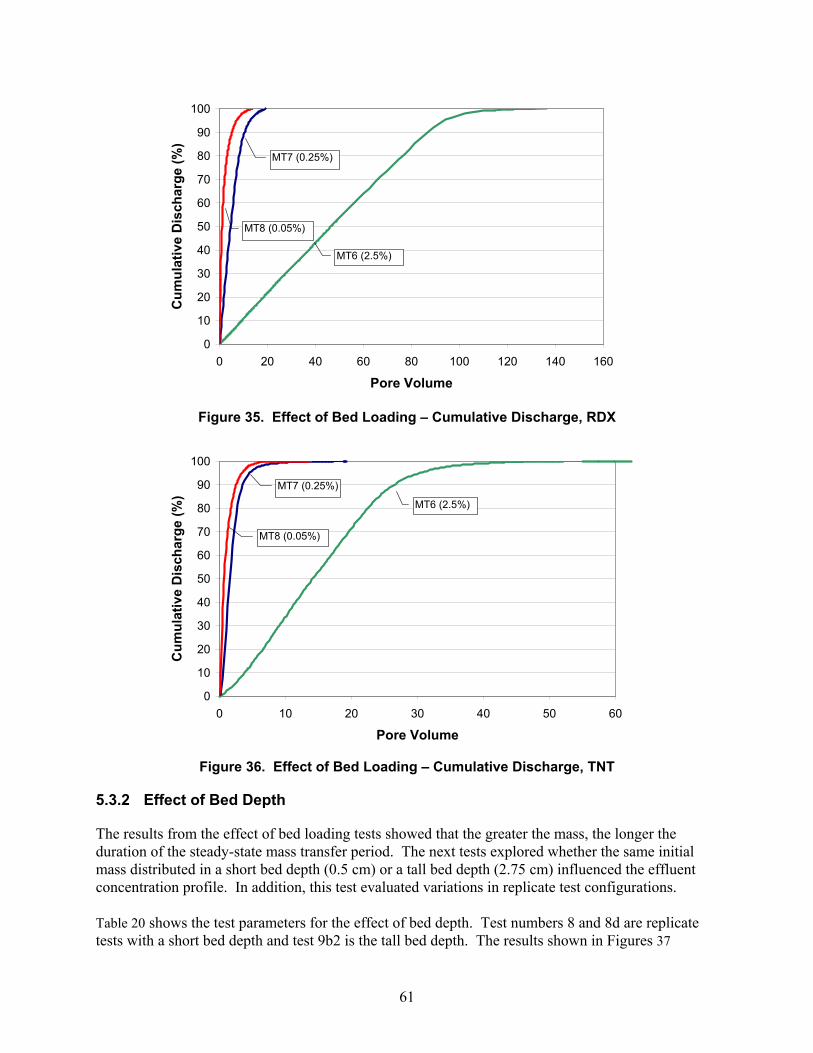
61
0
10
20
30
40
50
60
70
80
90
100
0 20 40 60 80 100 120 140 160
Pore Volume
Cum
ulat
ive
Dis
char
ge (%
)
MT6 (2.5%)
MT7 (0.25%)
MT8 (0.05%)
Figure 35. Effect of Bed Loading – Cumulative Discharge, RDX
0
10
20
30
40
50
60
70
80
90
100
0 10 20 30 40 50 60
Pore Volume
Cum
ulat
ive
Dis
char
ge (%
)
MT6 (2.5%)
MT7 (0.25%)
MT8 (0.05%)
Figure 36. Effect of Bed Loading – Cumulative Discharge, TNT
5.3.2 Effect of Bed Depth
The results from the effect of bed loading tests showed that the greater the mass, the longer the duration of the steady-state mass transfer period. The next tests explored whether the same initial mass distributed in a short bed depth (0.5 cm) or a tall bed depth (2.75 cm) influenced the effluent concentration profile. In addition, this test evaluated variations in replicate test configurations. Table 20 shows the test parameters for the effect of bed depth. Test numbers 8 and 8d are replicate tests with a short bed depth and test 9b2 is the tall bed depth. The results shown in Figures 37
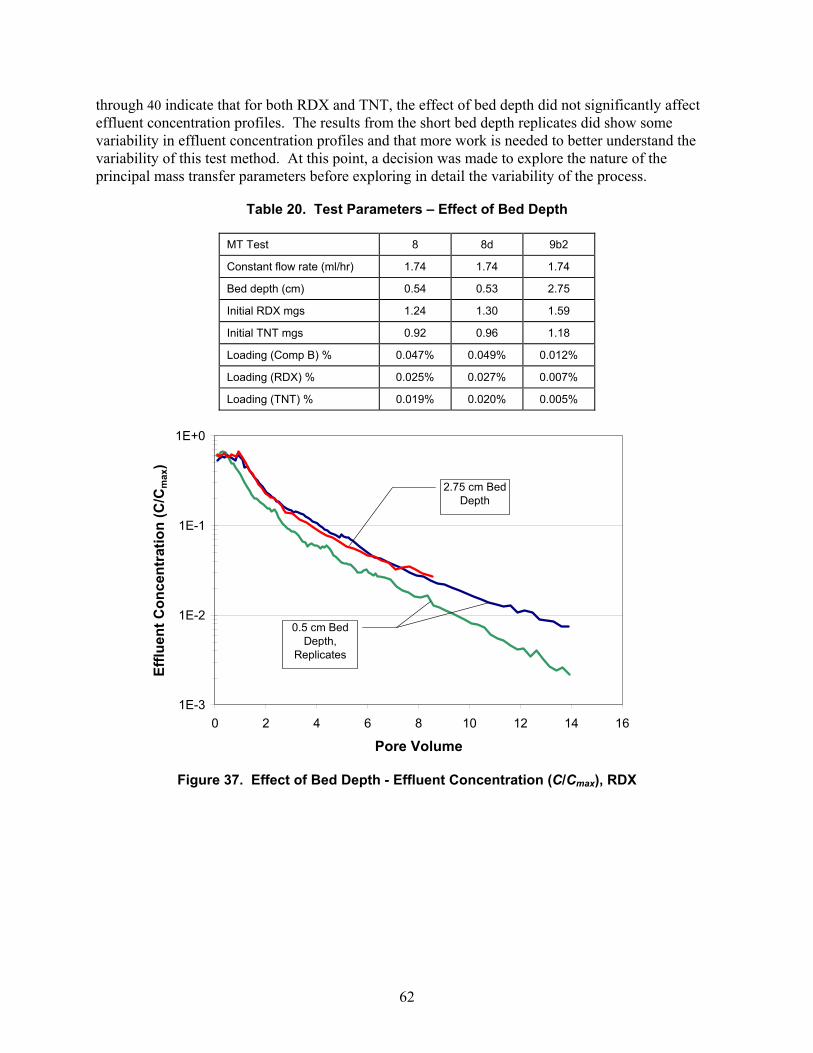
62
through 40 indicate that for both RDX and TNT, the effect of bed depth did not significantly affect effluent concentration profiles. The results from the short bed depth replicates did show some variability in effluent concentration profiles and that more work is needed to better understand the variability of this test method. At this point, a decision was made to explore the nature of the principal mass transfer parameters before exploring in detail the variability of the process.
Table 20. Test Parameters – Effect of Bed Depth
MT Test 8 8d 9b2
Constant flow rate (ml/hr) 1.74 1.74 1.74
Bed depth (cm) 0.54 0.53 2.75
Initial RDX mgs 1.24 1.30 1.59
Initial TNT mgs 0.92 0.96 1.18
Loading (Comp B) % 0.047% 0.049% 0.012%
Loading (RDX) % 0.025% 0.027% 0.007%
Loading (TNT) % 0.019% 0.020% 0.005%
1E-3
1E-2
1E-1
1E+0
0 2 4 6 8 10 12 14 16
Pore Volume
Efflu
ent C
once
ntra
tion
(C/C
max
)
2.75 cm Bed Depth
0.5 cm Bed Depth,
Replicates
Figure 37. Effect of Bed Depth - Effluent Concentration (C/Cmax), RDX
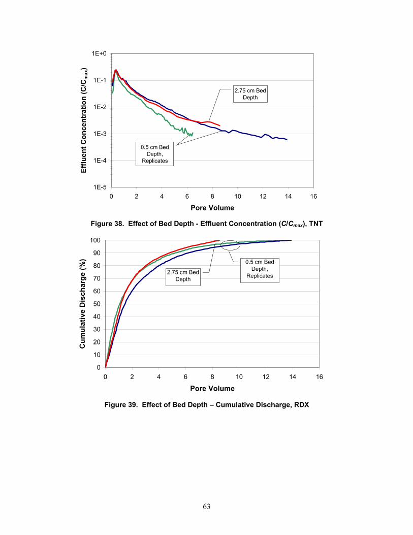
63
1E-5
1E-4
1E-3
1E-2
1E-1
1E+0
0 2 4 6 8 10 12 14 16
Pore Volume
Efflu
ent C
once
ntra
tion
(C/C
max
)2.75 cm Bed
Depth
0.5 cm Bed Depth,
Replicates
Figure 38. Effect of Bed Depth - Effluent Concentration (C/Cmax), TNT
0
10
20
30
40
50
60
70
80
90
100
0 2 4 6 8 10 12 14 16
Pore Volume
Cum
ulat
ive
Dis
char
ge (%
)
2.75 cm Bed Depth
0.5 cm Bed Depth,
Replicates
Figure 39. Effect of Bed Depth – Cumulative Discharge, RDX
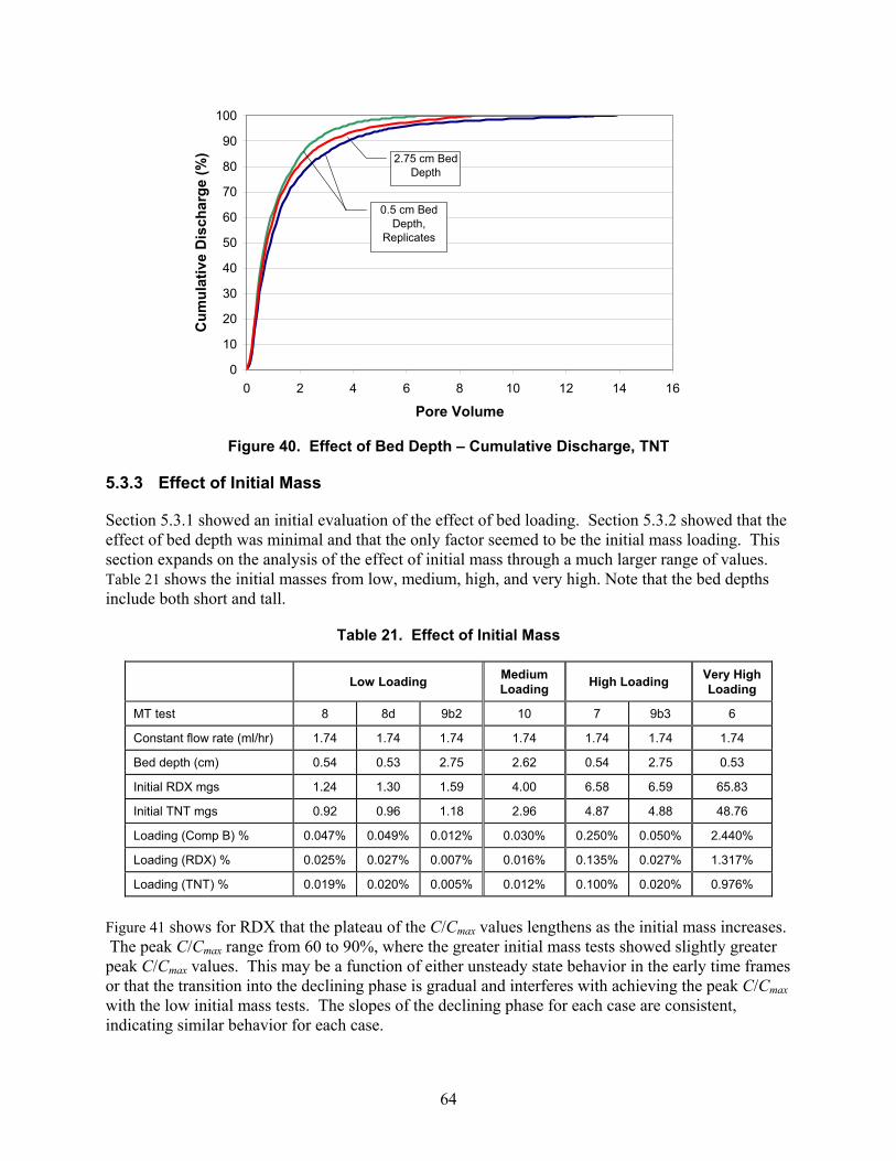
64
0
10
20
30
40
50
60
70
80
90
100
0 2 4 6 8 10 12 14 16
Pore Volume
Cum
ulat
ive
Dis
char
ge (%
) 2.75 cm Bed Depth
0.5 cm Bed Depth,
Replicates
Figure 40. Effect of Bed Depth – Cumulative Discharge, TNT
5.3.3 Effect of Initial Mass
Section 5.3.1 showed an initial evaluation of the effect of bed loading. Section 5.3.2 showed that the effect of bed depth was minimal and that the only factor seemed to be the initial mass loading. This section expands on the analysis of the effect of initial mass through a much larger range of values. Table 21 shows the initial masses from low, medium, high, and very high. Note that the bed depths include both short and tall.
Table 21. Effect of Initial Mass
Low Loading Medium Loading High Loading Very High
Loading
MT test 8 8d 9b2 10 7 9b3 6
Constant flow rate (ml/hr) 1.74 1.74 1.74 1.74 1.74 1.74 1.74
Bed depth (cm) 0.54 0.53 2.75 2.62 0.54 2.75 0.53
Initial RDX mgs 1.24 1.30 1.59 4.00 6.58 6.59 65.83
Initial TNT mgs 0.92 0.96 1.18 2.96 4.87 4.88 48.76
Loading (Comp B) % 0.047% 0.049% 0.012% 0.030% 0.250% 0.050% 2.440%
Loading (RDX) % 0.025% 0.027% 0.007% 0.016% 0.135% 0.027% 1.317%
Loading (TNT) % 0.019% 0.020% 0.005% 0.012% 0.100% 0.020% 0.976%
Figure 41 shows for RDX that the plateau of the C/Cmax values lengthens as the initial mass increases. The peak C/Cmax range from 60 to 90%, where the greater initial mass tests showed slightly greater peak C/Cmax values. This may be a function of either unsteady state behavior in the early time frames or that the transition into the declining phase is gradual and interferes with achieving the peak C/Cmax with the low initial mass tests. The slopes of the declining phase for each case are consistent, indicating similar behavior for each case.
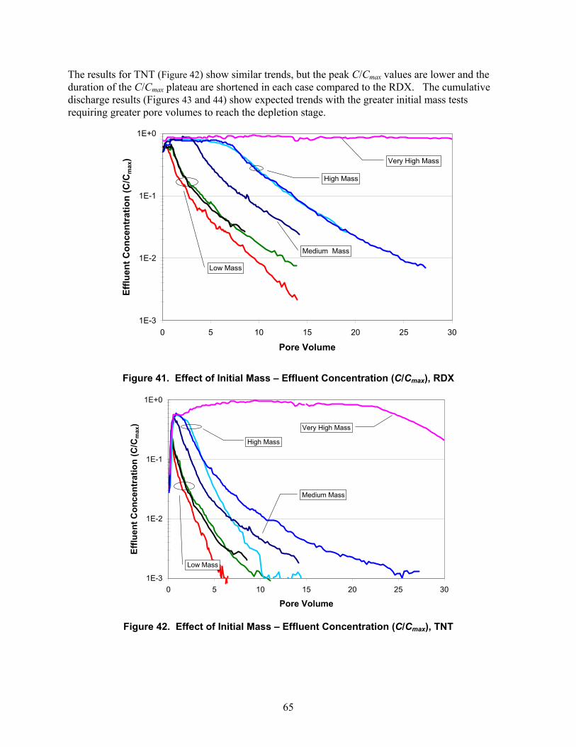
65
The results for TNT (Figure 42) show similar trends, but the peak C/Cmax values are lower and the duration of the C/Cmax plateau are shortened in each case compared to the RDX. The cumulative discharge results (Figures 43 and 44) show expected trends with the greater initial mass tests requiring greater pore volumes to reach the depletion stage.
1E-3
1E-2
1E-1
1E+0
0 5 10 15 20 25 30
Pore Volume
Efflu
ent C
once
ntra
tion
(C/C
max
)
Low Mass
High Mass
Medium Mass
Very High Mass
Figure 41. Effect of Initial Mass – Effluent Concentration (C/Cmax), RDX
1E-3
1E-2
1E-1
1E+0
0 5 10 15 20 25 30
Pore Volume
Efflu
ent C
once
ntra
tion
(C/C
max
)
High Mass
Low Mass
Medium Mass
Very High Mass
Figure 42. Effect of Initial Mass – Effluent Concentration (C/Cmax), TNT
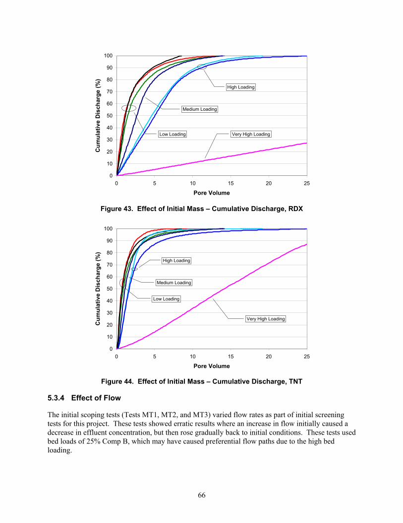
66
0
10
20
30
40
50
60
70
80
90
100
0 5 10 15 20 25
Pore Volume
Cum
ulat
ive
Dis
char
ge (%
)
Low Loading
High Loading
Very High Loading
Medium Loading
Figure 43. Effect of Initial Mass – Cumulative Discharge, RDX
0
10
20
30
40
50
60
70
80
90
100
0 5 10 15 20 25
Pore Volume
Cum
ulat
ive
Dis
char
ge (%
)
High Loading
Low Loading
Very High Loading
Medium Loading
Figure 44. Effect of Initial Mass – Cumulative Discharge, TNT
5.3.4 Effect of Flow
The initial scoping tests (Tests MT1, MT2, and MT3) varied flow rates as part of initial screening tests for this project. These tests showed erratic results where an increase in flow initially caused a decrease in effluent concentration, but then rose gradually back to initial conditions. These tests used bed loads of 25% Comp B, which may have caused preferential flow paths due to the high bed loading.
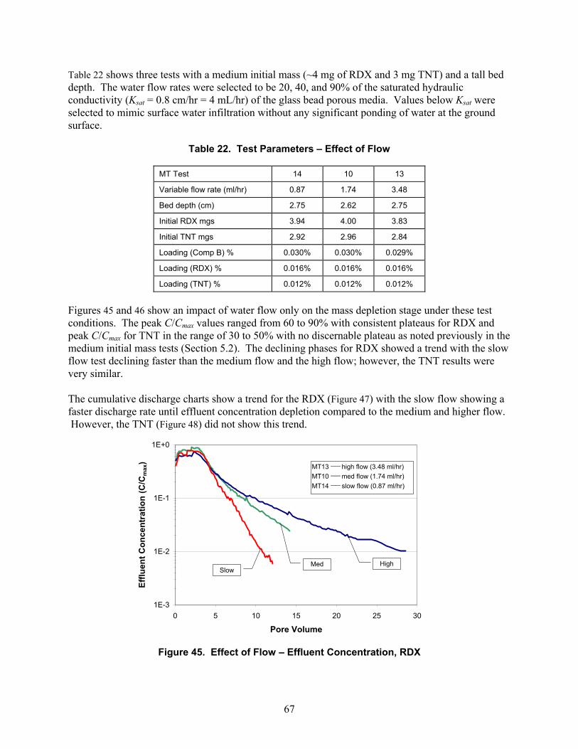
67
Table 22 shows three tests with a medium initial mass (~4 mg of RDX and 3 mg TNT) and a tall bed depth. The water flow rates were selected to be 20, 40, and 90% of the saturated hydraulic conductivity (Ksat = 0.8 cm/hr = 4 mL/hr) of the glass bead porous media. Values below Ksat were selected to mimic surface water infiltration without any significant ponding of water at the ground surface.
Table 22. Test Parameters – Effect of Flow
MT Test 14 10 13
Variable flow rate (ml/hr) 0.87 1.74 3.48
Bed depth (cm) 2.75 2.62 2.75
Initial RDX mgs 3.94 4.00 3.83
Initial TNT mgs 2.92 2.96 2.84
Loading (Comp B) % 0.030% 0.030% 0.029%
Loading (RDX) % 0.016% 0.016% 0.016%
Loading (TNT) % 0.012% 0.012% 0.012%
Figures 45 and 46 show an impact of water flow only on the mass depletion stage under these test conditions. The peak C/Cmax values ranged from 60 to 90% with consistent plateaus for RDX and peak C/Cmax for TNT in the range of 30 to 50% with no discernable plateau as noted previously in the medium initial mass tests (Section 5.2). The declining phases for RDX showed a trend with the slow flow test declining faster than the medium flow and the high flow; however, the TNT results were very similar. The cumulative discharge charts show a trend for the RDX (Figure 47) with the slow flow showing a faster discharge rate until effluent concentration depletion compared to the medium and higher flow. However, the TNT (Figure 48) did not show this trend.
1E-3
1E-2
1E-1
1E+0
0 5 10 15 20 25 30
Pore Volume
Efflu
ent C
once
ntra
tion
(C/C
max
) MT13 ____ high flow (3.48 ml/hr)MT10 ____ med flow (1.74 ml/hr)MT14 ____ slow flow (0.87 ml/hr)
SlowHighMed
Figure 45. Effect of Flow – Effluent Concentration, RDX
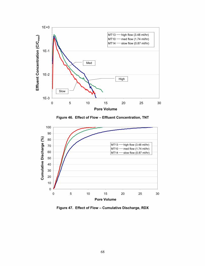
68
1E-3
1E-2
1E-1
1E+0
0 5 10 15 20 25 30
Pore Volume
Efflu
ent C
once
ntra
tion
(C/C
max
) MT13 ____ high flow (3.48 ml/hr)MT10 ____ med flow (1.74 ml/hr)MT14 ____ slow flow (0.87 ml/hr)
Slow
High
Med
Figure 46. Effect of Flow – Effluent Concentration, TNT
0
10
20
30
40
50
60
70
80
90
100
0 5 10 15 20 25 30
Pore Volume
Cum
ulat
ive
Dis
char
ge (%
)
MT13 ____ high flow (3.48 ml/hr)MT10 ____ med flow (1.74 ml/hr)MT14 ____ slow flow (0.87 ml/hr)
Figure 47. Effect of Flow – Cumulative Discharge, RDX
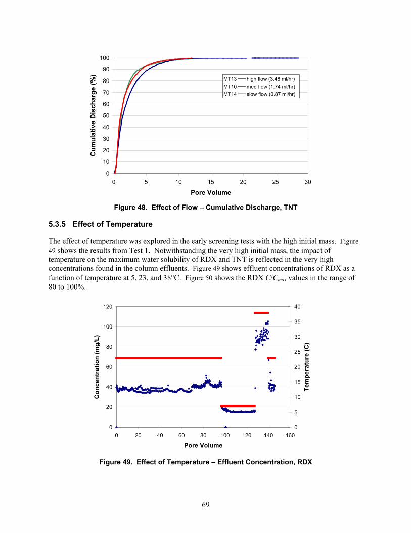
69
0
10
20
30
40
50
60
70
80
90
100
0 5 10 15 20 25 30
Pore Volume
Cum
ulat
ive
Dis
char
ge (%
)
MT13 ____ high flow (3.48 ml/hr)MT10 ____ med flow (1.74 ml/hr)MT14 ____ slow flow (0.87 ml/hr)
Figure 48. Effect of Flow – Cumulative Discharge, TNT
5.3.5 Effect of Temperature
The effect of temperature was explored in the early screening tests with the high initial mass. Figure 49 shows the results from Test 1. Notwithstanding the very high initial mass, the impact of temperature on the maximum water solubility of RDX and TNT is reflected in the very high concentrations found in the column effluents. Figure 49 shows effluent concentrations of RDX as a function of temperature at 5, 23, and 38°C. Figure 50 shows the RDX C/Cmax values in the range of 80 to 100%.
0
20
40
60
80
100
120
0 20 40 60 80 100 120 140 160
Pore Volume
Con
cent
ratio
n (m
g/L)
0
5
10
15
20
25
30
35
40Te
mpe
ratu
re (C
)
Figure 49. Effect of Temperature – Effluent Concentration, RDX
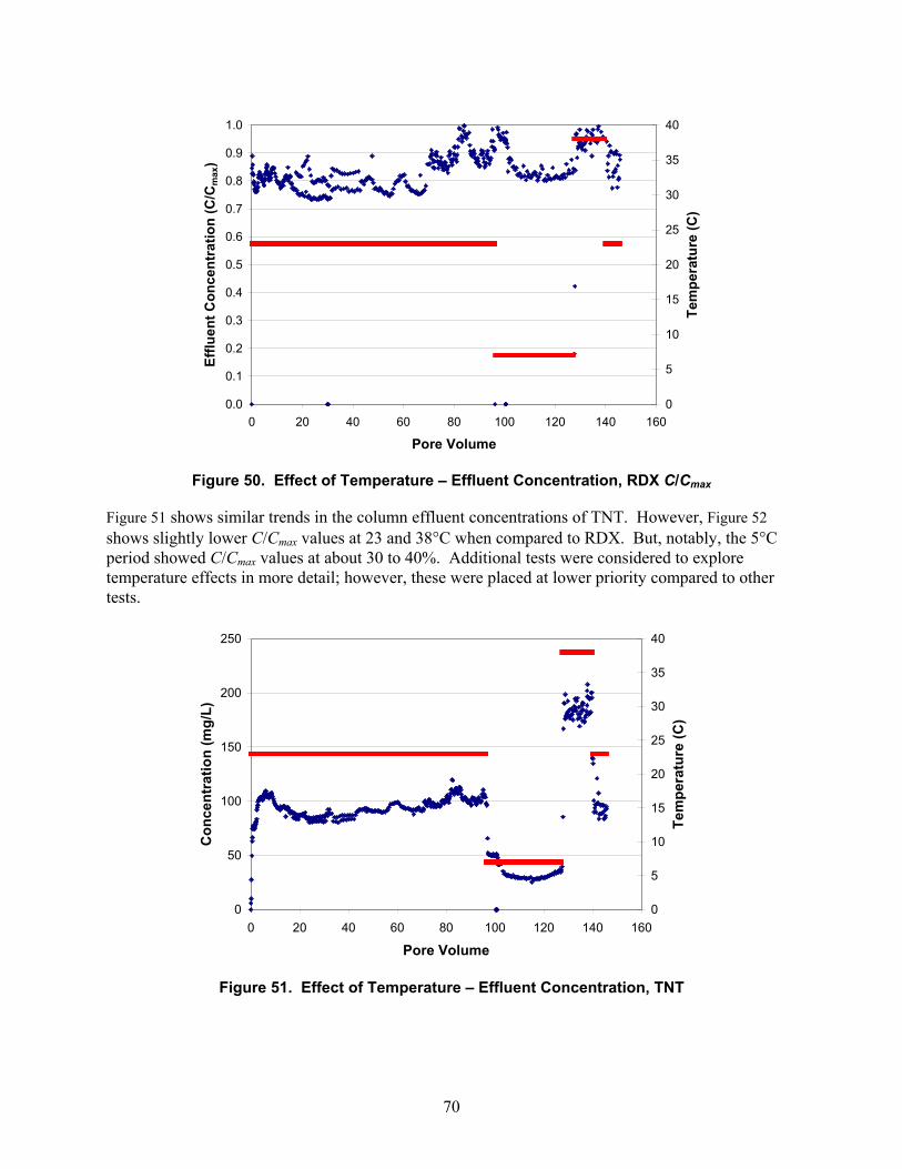
70
0.0
0.1
0.2
0.3
0.4
0.5
0.6
0.7
0.8
0.9
1.0
0 20 40 60 80 100 120 140 160
Pore Volume
Efflu
ent C
once
ntra
tion
(C/C
max
)
0
5
10
15
20
25
30
35
40
Tem
pera
ture
(C)
Figure 50. Effect of Temperature – Effluent Concentration, RDX C/Cmax
Figure 51 shows similar trends in the column effluent concentrations of TNT. However, Figure 52 shows slightly lower C/Cmax values at 23 and 38°C when compared to RDX. But, notably, the 5°C period showed C/Cmax values at about 30 to 40%. Additional tests were considered to explore temperature effects in more detail; however, these were placed at lower priority compared to other tests.
0
50
100
150
200
250
0 20 40 60 80 100 120 140 160
Pore Volume
Con
cent
ratio
n (m
g/L)
0
5
10
15
20
25
30
35
40
Tem
pera
ture
(C)
Figure 51. Effect of Temperature – Effluent Concentration, TNT
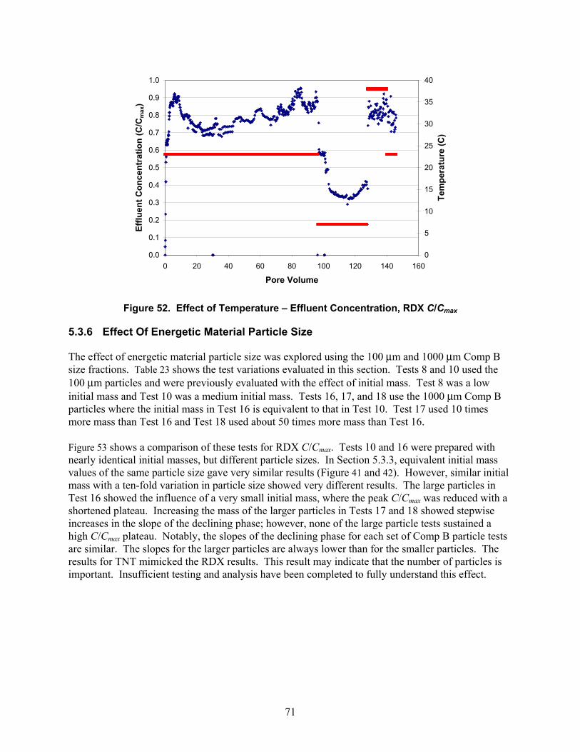
71
0.0
0.1
0.2
0.3
0.4
0.5
0.6
0.7
0.8
0.9
1.0
0 20 40 60 80 100 120 140 160
Pore Volume
Efflu
ent C
once
ntra
tion
(C/C
max
)
0
5
10
15
20
25
30
35
40
Tem
pera
ture
(C)
Figure 52. Effect of Temperature – Effluent Concentration, RDX C/Cmax
5.3.6 Effect Of Energetic Material Particle Size
The effect of energetic material particle size was explored using the 100 μm and 1000 μm Comp B size fractions. Table 23 shows the test variations evaluated in this section. Tests 8 and 10 used the 100 μm particles and were previously evaluated with the effect of initial mass. Test 8 was a low initial mass and Test 10 was a medium initial mass. Tests 16, 17, and 18 use the 1000 μm Comp B particles where the initial mass in Test 16 is equivalent to that in Test 10. Test 17 used 10 times more mass than Test 16 and Test 18 used about 50 times more mass than Test 16. Figure 53 shows a comparison of these tests for RDX C/Cmax. Tests 10 and 16 were prepared with nearly identical initial masses, but different particle sizes. In Section 5.3.3, equivalent initial mass values of the same particle size gave very similar results (Figure 41 and 42). However, similar initial mass with a ten-fold variation in particle size showed very different results. The large particles in Test 16 showed the influence of a very small initial mass, where the peak C/Cmax was reduced with a shortened plateau. Increasing the mass of the larger particles in Tests 17 and 18 showed stepwise increases in the slope of the declining phase; however, none of the large particle tests sustained a high C/Cmax plateau. Notably, the slopes of the declining phase for each set of Comp B particle tests are similar. The slopes for the larger particles are always lower than for the smaller particles. The results for TNT mimicked the RDX results. This result may indicate that the number of particles is important. Insufficient testing and analysis have been completed to fully understand this effect.
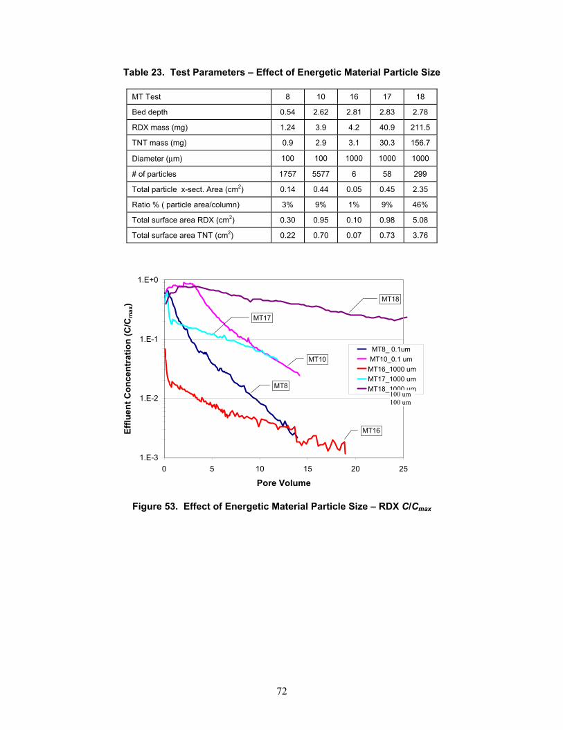
72
Table 23. Test Parameters – Effect of Energetic Material Particle Size
MT Test 8 10 16 17 18
Bed depth 0.54 2.62 2.81 2.83 2.78
RDX mass (mg) 1.24 3.9 4.2 40.9 211.5
TNT mass (mg) 0.9 2.9 3.1 30.3 156.7
Diameter (μm) 100 100 1000 1000 1000
# of particles 1757 5577 6 58 299
Total particle x-sect. Area (cm2) 0.14 0.44 0.05 0.45 2.35
Ratio % ( particle area/column) 3% 9% 1% 9% 46%
Total surface area RDX (cm2) 0.30 0.95 0.10 0.98 5.08
Total surface area TNT (cm2) 0.22 0.70 0.07 0.73 3.76
1.E-3
1.E-2
1.E-1
1.E+0
0 5 10 15 20 25
Pore Volume
Efflu
ent C
once
ntra
tion
(C/C
max
)
MT8_ 0.1um MT10_0.1 umMT16_1000 umMT17_1000 umMT18_1000 um
MT16
MT17
MT18
MT8
MT10
Figure 53. Effect of Energetic Material Particle Size – RDX C/Cmax
100 um 100 um
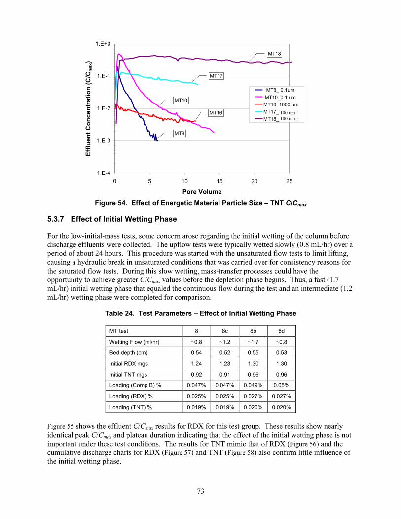
73
1.E-4
1.E-3
1.E-2
1.E-1
1.E+0
0 5 10 15 20 25
Pore Volume
Efflu
ent C
once
ntra
tion
(C/C
max
) MT8_ 0.1um MT10_0.1 umMT16_1000 umMT17_1000 umMT18_1000 um
MT16
MT17
MT18
MT8
MT10
Figure 54. Effect of Energetic Material Particle Size – TNT C/Cmax
5.3.7 Effect of Initial Wetting Phase
For the low-initial-mass tests, some concern arose regarding the initial wetting of the column before discharge effluents were collected. The upflow tests were typically wetted slowly (0.8 mL/hr) over a period of about 24 hours. This procedure was started with the unsaturated flow tests to limit lifting, causing a hydraulic break in unsaturated conditions that was carried over for consistency reasons for the saturated flow tests. During this slow wetting, mass-transfer processes could have the opportunity to achieve greater C/Cmax values before the depletion phase begins. Thus, a fast (1.7 mL/hr) initial wetting phase that equaled the continuous flow during the test and an intermediate (1.2 mL/hr) wetting phase were completed for comparison.
Table 24. Test Parameters – Effect of Initial Wetting Phase
MT test 8 8c 8b 8d
Wetting Flow (ml/hr) ~0.8 ~1.2 ~1.7 ~0.8
Bed depth (cm) 0.54 0.52 0.55 0.53
Initial RDX mgs 1.24 1.23 1.30 1.30
Initial TNT mgs 0.92 0.91 0.96 0.96
Loading (Comp B) % 0.047% 0.047% 0.049% 0.05%
Loading (RDX) % 0.025% 0.025% 0.027% 0.027%
Loading (TNT) % 0.019% 0.019% 0.020% 0.020%
Figure 55 shows the effluent C/Cmax results for RDX for this test group. These results show nearly identical peak C/Cmax and plateau duration indicating that the effect of the initial wetting phase is not important under these test conditions. The results for TNT mimic that of RDX (Figure 56) and the cumulative discharge charts for RDX (Figure 57) and TNT (Figure 58) also confirm little influence of the initial wetting phase.
100 um 100 um
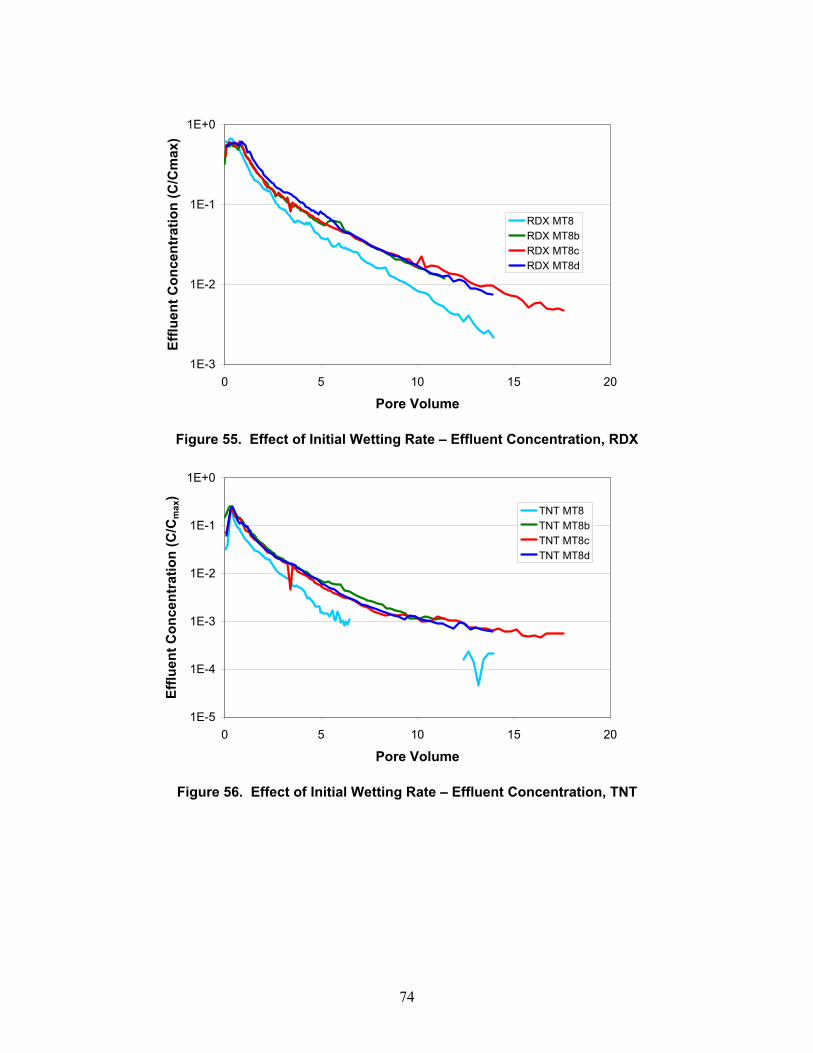
74
1E-3
1E-2
1E-1
1E+0
0 5 10 15 20
Pore Volume
Efflu
ent C
once
ntra
tion
(C/C
max
)
RDX MT8RDX MT8bRDX MT8cRDX MT8d
Figure 55. Effect of Initial Wetting Rate – Effluent Concentration, RDX
1E-5
1E-4
1E-3
1E-2
1E-1
1E+0
0 5 10 15 20
Pore Volume
Efflu
ent C
once
ntra
tion
(C/C
max
)
TNT MT8TNT MT8bTNT MT8cTNT MT8d
Figure 56. Effect of Initial Wetting Rate – Effluent Concentration, TNT
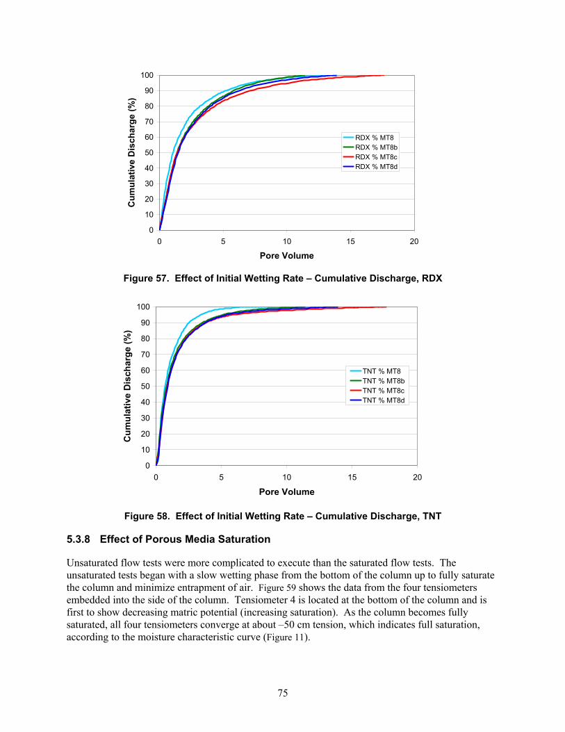
75
0
10
20
30
40
50
60
70
80
90
100
0 5 10 15 20
Pore Volume
Cum
ulat
ive
Dis
char
ge (%
)RDX % MT8RDX % MT8bRDX % MT8cRDX % MT8d
Figure 57. Effect of Initial Wetting Rate – Cumulative Discharge, RDX
0
10
20
30
40
50
60
70
80
90
100
0 5 10 15 20
Pore Volume
Cum
ulat
ive
Dis
char
ge (%
)
TNT % MT8TNT % MT8bTNT % MT8cTNT % MT8d
Figure 58. Effect of Initial Wetting Rate – Cumulative Discharge, TNT
5.3.8 Effect of Porous Media Saturation
Unsaturated flow tests were more complicated to execute than the saturated flow tests. The unsaturated tests began with a slow wetting phase from the bottom of the column up to fully saturate the column and minimize entrapment of air. Figure 59 shows the data from the four tensiometers embedded into the side of the column. Tensiometer 4 is located at the bottom of the column and is first to show decreasing matric potential (increasing saturation). As the column becomes fully saturated, all four tensiometers converge at about –50 cm tension, which indicates full saturation, according to the moisture characteristic curve (Figure 11).
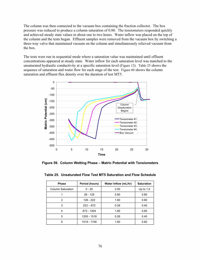
76
The column was then connected to the vacuum box containing the fraction collector. The box pressure was reduced to produce a column saturation of 0.80. The tensiometers responded quickly and achieved steady state values in about one to two hours. Water inflow was placed on the top of the column and the tests began. Effluent samples were removed from the vacuum box by switching a three-way valve that maintained vacuum on the column and simultaneously relieved vacuum from the box. The tests were run in sequential mode where a saturation value was maintained until effluent concentrations appeared at steady state. Water inflow for each saturation level was matched to the unsaturated hydraulic conductivity at a specific saturation level (Figure 12). Table 25 shows the sequence of saturation and water flow for each stage of the test. Figure 60 shows the column saturation and effluent flux density over the duration of test MT5.
-500
-450
-400
-350
-300
-250
-200
-150
-100
-50
0
0 5 10 15 20 25 30
Time
Mat
ric P
oten
tial (
cm)
Tensiometer #1Tensiometer #2Tensiometer #3Tensiometer #4Box Vacuum
Column Desaturation
Begins
Figure 59. Column Wetting Phase – Matric Potential with Tensiometers
Table 25. Unsaturated Flow Test MT5 Saturation and Flow Schedule
Phase Period (hours) Water Inflow (mL/hr) Saturation
Column Saturation 0 - 20 3.50 Up to 1.0
1 26 - 125 5.80 0.80
2 126 - 222 1.60 0.60
3 223 – 672 0.26 0.40
4 673 - 1204 1.60 0.60
5 1205 - 1518 0.26 0.40
6 1519 - 1746 1.60 0.60
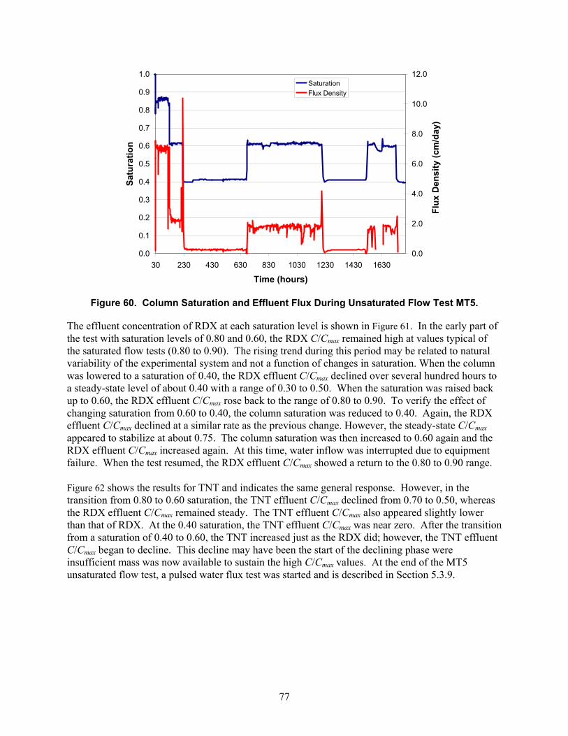
77
0.0
0.1
0.2
0.3
0.4
0.5
0.6
0.7
0.8
0.9
1.0
30 230 430 630 830 1030 1230 1430 1630
Time (hours)
Satu
ratio
n
0.0
2.0
4.0
6.0
8.0
10.0
12.0
Flux
Den
sity
(cm
/day
)
SaturationFlux Density
Figure 60. Column Saturation and Effluent Flux During Unsaturated Flow Test MT5.
The effluent concentration of RDX at each saturation level is shown in Figure 61. In the early part of the test with saturation levels of 0.80 and 0.60, the RDX C/Cmax remained high at values typical of the saturated flow tests (0.80 to 0.90). The rising trend during this period may be related to natural variability of the experimental system and not a function of changes in saturation. When the column was lowered to a saturation of 0.40, the RDX effluent C/Cmax declined over several hundred hours to a steady-state level of about 0.40 with a range of 0.30 to 0.50. When the saturation was raised back up to 0.60, the RDX effluent C/Cmax rose back to the range of 0.80 to 0.90. To verify the effect of changing saturation from 0.60 to 0.40, the column saturation was reduced to 0.40. Again, the RDX effluent C/Cmax declined at a similar rate as the previous change. However, the steady-state C/Cmax appeared to stabilize at about 0.75. The column saturation was then increased to 0.60 again and the RDX effluent C/Cmax increased again. At this time, water inflow was interrupted due to equipment failure. When the test resumed, the RDX effluent C/Cmax showed a return to the 0.80 to 0.90 range. Figure 62 shows the results for TNT and indicates the same general response. However, in the transition from 0.80 to 0.60 saturation, the TNT effluent C/Cmax declined from 0.70 to 0.50, whereas the RDX effluent C/Cmax remained steady. The TNT effluent C/Cmax also appeared slightly lower than that of RDX. At the 0.40 saturation, the TNT effluent C/Cmax was near zero. After the transition from a saturation of 0.40 to 0.60, the TNT increased just as the RDX did; however, the TNT effluent C/Cmax began to decline. This decline may have been the start of the declining phase were insufficient mass was now available to sustain the high C/Cmax values. At the end of the MT5 unsaturated flow test, a pulsed water flux test was started and is described in Section 5.3.9.
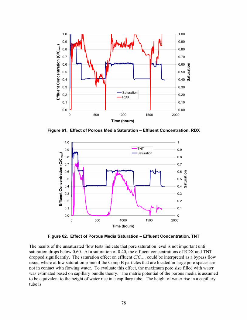
78
0.0
0.1
0.2
0.3
0.4
0.5
0.6
0.7
0.8
0.9
1.0
0 500 1000 1500 2000
Time (hours)
Efflu
ent C
once
ntra
tion
(C/C
max
)
0.00
0.10
0.20
0.30
0.40
0.50
0.60
0.70
0.80
0.90
1.00
Satu
ratio
n
SaturationRDX
Figure 61. Effect of Porous Media Saturation – Effluent Concentration, RDX
0.0
0.1
0.2
0.3
0.4
0.5
0.6
0.7
0.8
0.9
1.0
0 500 1000 1500 2000
Time (hours)
Efflu
ent C
once
ntra
tion
(C/C
max
)
0
0.1
0.2
0.3
0.4
0.5
0.6
0.7
0.8
0.9
1
Satu
ratio
n
TNTSaturation
Figure 62. Effect of Porous Media Saturation – Effluent Concentration, TNT
The results of the unsaturated flow tests indicate that pore saturation level is not important until saturation drops below 0.60. At a saturation of 0.40, the effluent concentrations of RDX and TNT dropped significantly. The saturation effect on effluent C/Cmax could be interpreted as a bypass flow issue, where at low saturation some of the Comp B particles that are located in large pore spaces are not in contact with flowing water. To evaluate this effect, the maximum pore size filled with water was estimated based on capillary bundle theory. The matric potential of the porous media is assumed to be equivalent to the height of water rise in a capillary tube. The height of water rise in a capillary tube is
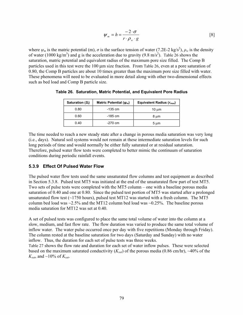
79
gr
hw
m ⋅⋅⋅−==
ρσψ 2
[8]
where ψm is the matric potential (m), σ is the surface tension of water (7.2E-2 kg/s2), ρw is the density of water (1000 kg/m3) and g is the acceleration due to gravity (9.8 m/s2). Table 26 shows the saturation, matric potential and equivalent radius of the maximum pore size filled. The Comp B particles used in this test were the 100 μm size fraction. From Table 26, even at a pore saturation of 0.80, the Comp B particles are about 10 times greater than the maximum pore size filled with water. These phenomena will need to be evaluated in more detail along with other two-dimensional effects such as bed load and Comp B particle size.
Table 26. Saturation, Matric Potential, and Equivalent Pore Radius
Saturation (Sl) Matric Potential (ψm) Equivalent Radius (rmax)
0.80 -135 cm 10 μm
0.60 -185 cm 8 μm
0.40 -270 cm 5 μm
The time needed to reach a new steady state after a change in porous media saturation was very long (i.e., days). Natural soil systems would not remain at these intermediate saturation levels for such long periods of time and would normally be either fully saturated or at residual saturation. Therefore, pulsed water flow tests were completed to better mimic the continuum of saturation conditions during periodic rainfall events. 5.3.9 Effect Of Pulsed Water Flow
The pulsed water flow tests used the same unsaturated flow columns and test equipment as described in Section 5.3.8. Pulsed test MT5 was initiated at the end of the unsaturated flow part of test MT5. Two sets of pulse tests were completed with the MT5 column – one with a baseline porous media saturation of 0.40 and one at 0.80. Since the pulsed test portion of MT5 was started after a prolonged unsaturated flow test (~1750 hours), pulsed test MT12 was started with a fresh column. The MT5 column bed load was ~2.5% and the MT12 column bed load was ~0.25%. The baseline porous media saturation for MT12 was set at 0.40. A set of pulsed tests was configured to place the same total volume of water into the column at a slow, medium, and fast flow rate. The flow duration was varied to produce the same total volume of inflow water. The water pulse occurred once per day with five repetitions (Monday through Friday). The column rested at the baseline saturation for two days (Saturday and Sunday) with no water inflow. Thus, the duration for each set of pulse tests was three weeks. Table 27 shows the flow rate and duration for each set of water inflow pulses. These were selected based on the maximum saturated conductivity (Ksat) of the porous media (0.86 cm/hr), ~40% of the Ksat, and ~10% of Ksat.
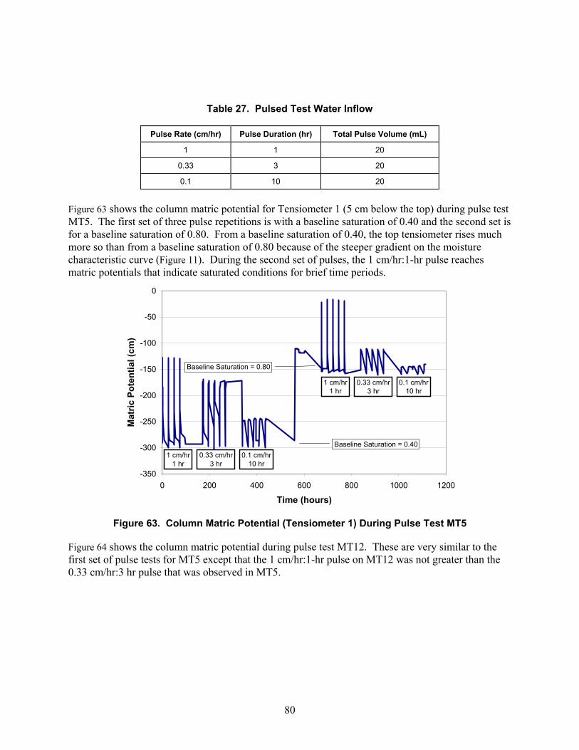
80
Table 27. Pulsed Test Water Inflow
Pulse Rate (cm/hr) Pulse Duration (hr) Total Pulse Volume (mL)
1 1 20
0.33 3 20
0.1 10 20
Figure 63 shows the column matric potential for Tensiometer 1 (5 cm below the top) during pulse test MT5. The first set of three pulse repetitions is with a baseline saturation of 0.40 and the second set is for a baseline saturation of 0.80. From a baseline saturation of 0.40, the top tensiometer rises much more so than from a baseline saturation of 0.80 because of the steeper gradient on the moisture characteristic curve (Figure 11). During the second set of pulses, the 1 cm/hr:1-hr pulse reaches matric potentials that indicate saturated conditions for brief time periods.
-350
-300
-250
-200
-150
-100
-50
0
0 200 400 600 800 1000 1200
Time (hours)
Mat
ric P
oten
tial (
cm)
Baseline Saturation = 0.40
Baseline Saturation = 0.80
1 cm/hr1 hr
0.33 cm/hr3 hr
0.1 cm/hr10 hr
1 cm/hr1 hr
0.33 cm/hr3 hr
0.1 cm/hr10 hr
Figure 63. Column Matric Potential (Tensiometer 1) During Pulse Test MT5
Figure 64 shows the column matric potential during pulse test MT12. These are very similar to the first set of pulse tests for MT5 except that the 1 cm/hr:1-hr pulse on MT12 was not greater than the 0.33 cm/hr:3 hr pulse that was observed in MT5.
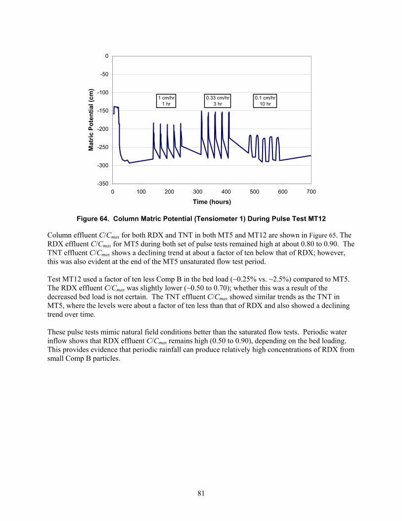
81
-350
-300
-250
-200
-150
-100
-50
0
0 100 200 300 400 500 600 700
Time (hours)
Mat
ric P
oten
tial (
cm)
1 cm/hr1 hr
0.33 cm/hr3 hr
0.1 cm/hr10 hr
Figure 64. Column Matric Potential (Tensiometer 1) During Pulse Test MT12
Column effluent C/Cmax for both RDX and TNT in both MT5 and MT12 are shown in Figure 65. The RDX effluent C/Cmax for MT5 during both set of pulse tests remained high at about 0.80 to 0.90. The TNT effluent C/Cmax shows a declining trend at about a factor of ten below that of RDX; however, this was also evident at the end of the MT5 unsaturated flow test period. Test MT12 used a factor of ten less Comp B in the bed load (~0.25% vs. ~2.5%) compared to MT5. The RDX effluent C/Cmax was slightly lower (~0.50 to 0.70); whether this was a result of the decreased bed load is not certain. The TNT effluent C/Cmax showed similar trends as the TNT in MT5, where the levels were about a factor of ten less than that of RDX and also showed a declining trend over time. These pulse tests mimic natural field conditions better than the saturated flow tests. Periodic water inflow shows that RDX effluent C/Cmax remains high (0.50 to 0.90), depending on the bed loading. This provides evidence that periodic rainfall can produce relatively high concentrations of RDX from small Comp B particles.
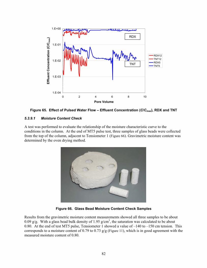
82
1.E-04
1.E-03
1.E-02
1.E-01
1.E+00
0 2 4 6 8 10
Pore Volume
Efflu
ent C
once
ntra
tion
(C/C
max
)
RDX12TNT12RDX5TNT5
Figure 65. Effect of Pulsed Water Flow – Effluent Concentration (C/Cmax), RDX and TNT
5.3.9.1 Moisture Content Check
A test was performed to evaluate the relationship of the moisture characteristic curve to the conditions in the column. At the end of MT5 pulse test, three samples of glass beads were collected from the top of the column, adjacent to Tensiometer 1 (Figure 66). Gravimetric moisture content was determined by the oven drying method.
Figure 66. Glass Bead Moisture Content Check Samples
Results from the gravimetric moisture content measurements showed all three samples to be about 0.09 g/g. With a glass bead bulk density of 1.95 g/cm3, the saturation was calculated to be about 0.80. At the end of test MT5 pulse, Tensiometer 1 showed a value of –140 to –150 cm tension. This corresponds to a moisture content of 0.79 to 0.73 g/g (Figure 11), which is in good agreement with the measured moisture content of 0.80.
RDX
TNT
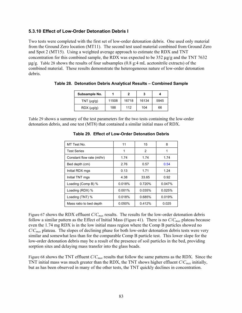
83
5.3.10 Effect of Low-Order Detonation Debris I
Two tests were completed with the first set of low-order detonation debris. One used only material from the Ground Zero location (MT11). The second test used material combined from Ground Zero and Spot 2 (MT15). Using a weighted average approach to estimate the RDX and TNT concentration for this combined sample, the RDX was expected to be 352 μg/g and the TNT 7632 μg/g. Table 28 shows the results of four subsamples (0.8 g:4 mL acetonitrile extracts) of the combined material. These results demonstrate the heterogeneous nature of low-order detonation debris.
Table 28. Detonation Debris Analytical Results – Combined Sample
Subsample No. 1 2 3 4
TNT (μg/g) 11508 16718 16134 5945
RDX (μg/g) 188 112 104 66
Table 29 shows a summary of the test parameters for the two tests containing the low-order detonation debris, and one test (MT8) that contained a similar initial mass of RDX.
Table 29. Effect of Low-Order Detonation Debris
MT Test No. 11 15 8
Test Series 1 2 1
Constant flow rate (ml/hr) 1.74 1.74 1.74
Bed depth (cm) 2.76 0.57 0.54
Initial RDX mgs 0.13 1.71 1.24
Initial TNT mgs 4.38 33.65 0.92
Loading (Comp B) % 0.018% 0.720% 0.047%
Loading (RDX) % 0.001% 0.035% 0.025%
Loading (TNT) % 0.018% 0.685% 0.019%
Mass ratio to bed depth 0.050% 0.412% 0.025
Figure 67 shows the RDX effluent C/Cmax results. The results for the low-order detonation debris follow a similar pattern as the Effect of Initial Mass (Figure 41). There is no C/Cmax plateau because even the 1.74 mg RDX is in the low initial mass region where the Comp B particles showed no C/Cmax plateau. The slopes of declining phase for both low-order detonation debris tests were very similar and somewhat less than for the comparable Comp B particle test. This lower slope for the low-order detonation debris may be a result of the presence of soil particles in the bed, providing sorption sites and delaying mass transfer into the glass beads. Figure 68 shows the TNT effluent C/Cmax results that follow the same patterns as the RDX. Since the TNT initial mass was much greater than the RDX, the TNT shows higher effluent C/Cmax initially, but as has been observed in many of the other tests, the TNT quickly declines in concentration.
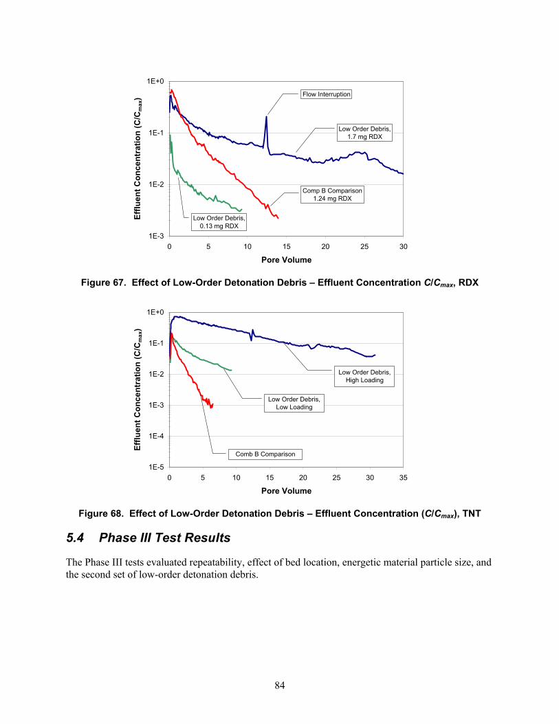
84
1E-3
1E-2
1E-1
1E+0
0 5 10 15 20 25 30
Pore Volume
Efflu
ent C
once
ntra
tion
(C/C
max
)Low Order Debris,
1.7 mg RDX
Comp B Comparison1.24 mg RDX
Low Order Debris, 0.13 mg RDX
Flow Interruption
Figure 67. Effect of Low-Order Detonation Debris – Effluent Concentration C/Cmax, RDX
1E-5
1E-4
1E-3
1E-2
1E-1
1E+0
0 5 10 15 20 25 30 35
Pore Volume
Efflu
ent C
once
ntra
tion
(C/C
max
)
Low Order Debris, High Loading
Low Order Debris, Low Loading
Comb B Comparison
Figure 68. Effect of Low-Order Detonation Debris – Effluent Concentration (C/Cmax), TNT
5.4 Phase III Test Results
The Phase III tests evaluated repeatability, effect of bed location, energetic material particle size, and the second set of low-order detonation debris.
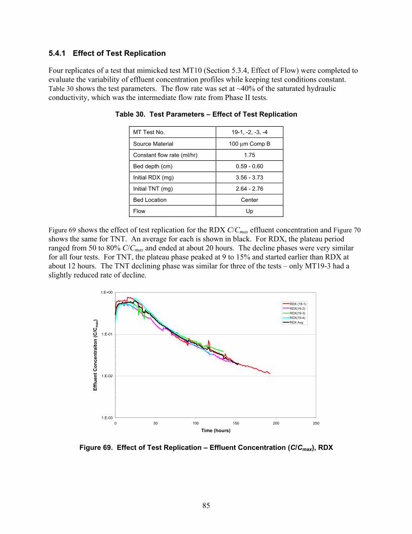
85
5.4.1 Effect of Test Replication
Four replicates of a test that mimicked test MT10 (Section 5.3.4, Effect of Flow) were completed to evaluate the variability of effluent concentration profiles while keeping test conditions constant. Table 30 shows the test parameters. The flow rate was set at ~40% of the saturated hydraulic conductivity, which was the intermediate flow rate from Phase II tests.
Table 30. Test Parameters – Effect of Test Replication
MT Test No. 19-1, -2, -3, -4
Source Material 100 μm Comp B
Constant flow rate (ml/hr) 1.75
Bed depth (cm) 0.59 - 0.60
Initial RDX (mg) 3.56 - 3.73
Initial TNT (mg) 2.64 - 2.76
Bed Location Center
Flow Up
Figure 69 shows the effect of test replication for the RDX C/Cmax effluent concentration and Figure 70 shows the same for TNT. An average for each is shown in black. For RDX, the plateau period ranged from 50 to 80% C/Cmax and ended at about 20 hours. The decline phases were very similar for all four tests. For TNT, the plateau phase peaked at 9 to 15% and started earlier than RDX at about 12 hours. The TNT declining phase was similar for three of the tests – only MT19-3 had a slightly reduced rate of decline.
1.E-03
1.E-02
1.E-01
1.E+00
0 50 100 150 200 250
Time (hours)
Efflu
ent C
once
ntra
iton
(C/C
max
)
RDX (19-1)RDX(19-2)RDX(19-3)RDX(19-4)RDX Avg
Figure 69. Effect of Test Replication – Effluent Concentration (C/Cmax), RDX
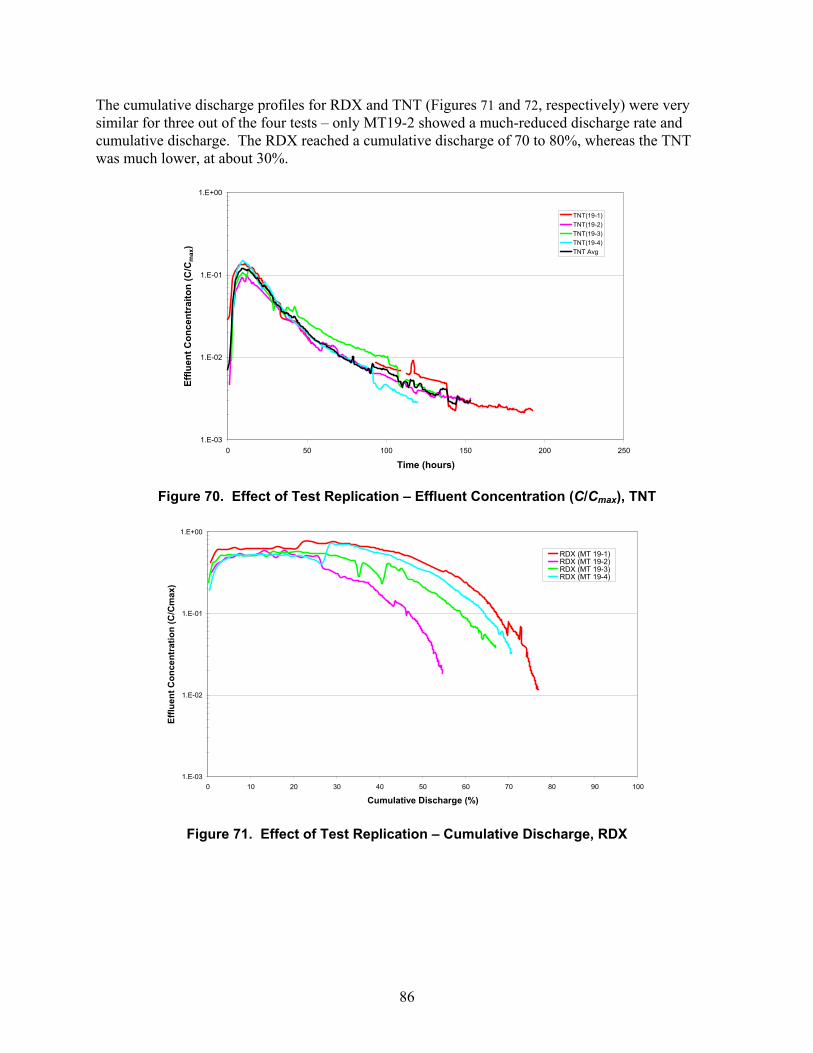
86
The cumulative discharge profiles for RDX and TNT (Figures 71 and 72, respectively) were very similar for three out of the four tests – only MT19-2 showed a much-reduced discharge rate and cumulative discharge. The RDX reached a cumulative discharge of 70 to 80%, whereas the TNT was much lower, at about 30%.
1.E-03
1.E-02
1.E-01
1.E+00
0 50 100 150 200 250
Time (hours)
Efflu
ent C
once
ntra
iton
(C/C
max
)
TNT(19-1)TNT(19-2)TNT(19-3)TNT(19-4)TNT Avg
Figure 70. Effect of Test Replication – Effluent Concentration (C/Cmax), TNT
1.E-03
1.E-02
1.E-01
1.E+00
0 10 20 30 40 50 60 70 80 90 100
Cumulative Discharge (%)
Efflu
ent C
once
ntra
tion
(C/C
max
)
RDX (MT 19-1)RDX (MT 19-2)RDX (MT 19-3)RDX (MT 19-4)
Figure 71. Effect of Test Replication – Cumulative Discharge, RDX
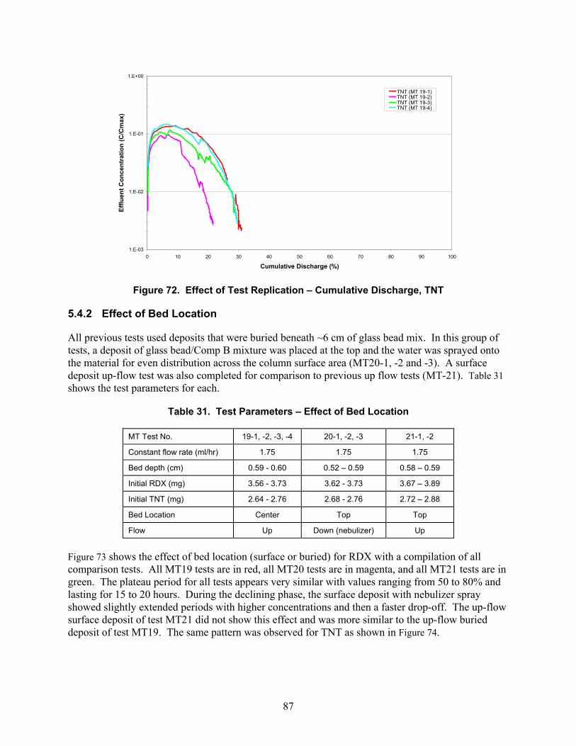
87
1.E-03
1.E-02
1.E-01
1.E+00
0 10 20 30 40 50 60 70 80 90 100
Cumulative Discharge (%)
Efflu
ent C
once
ntra
tion
(C/C
max
)
TNT (MT 19-1)TNT (MT 19-2)TNT (MT 19-3)TNT (MT 19-4)
Figure 72. Effect of Test Replication – Cumulative Discharge, TNT
5.4.2 Effect of Bed Location
All previous tests used deposits that were buried beneath ~6 cm of glass bead mix. In this group of tests, a deposit of glass bead/Comp B mixture was placed at the top and the water was sprayed onto the material for even distribution across the column surface area (MT20-1, -2 and -3). A surface deposit up-flow test was also completed for comparison to previous up flow tests (MT-21). Table 31 shows the test parameters for each.
Table 31. Test Parameters – Effect of Bed Location
MT Test No. 19-1, -2, -3, -4 20-1, -2, -3 21-1, -2
Constant flow rate (ml/hr) 1.75 1.75 1.75
Bed depth (cm) 0.59 - 0.60 0.52 – 0.59 0.58 – 0.59
Initial RDX (mg) 3.56 - 3.73 3.62 - 3.73 3.67 – 3.89
Initial TNT (mg) 2.64 - 2.76 2.68 - 2.76 2.72 – 2.88
Bed Location Center Top Top
Flow Up Down (nebulizer) Up
Figure 73 shows the effect of bed location (surface or buried) for RDX with a compilation of all comparison tests. All MT19 tests are in red, all MT20 tests are in magenta, and all MT21 tests are in green. The plateau period for all tests appears very similar with values ranging from 50 to 80% and lasting for 15 to 20 hours. During the declining phase, the surface deposit with nebulizer spray showed slightly extended periods with higher concentrations and then a faster drop-off. The up-flow surface deposit of test MT21 did not show this effect and was more similar to the up-flow buried deposit of test MT19. The same pattern was observed for TNT as shown in Figure 74.
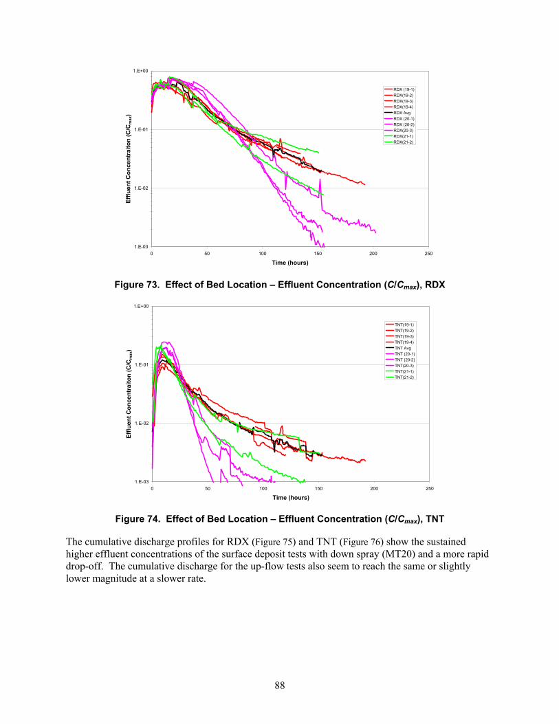
88
1.E-03
1.E-02
1.E-01
1.E+00
0 50 100 150 200 250
Time (hours)
Efflu
ent C
once
ntra
iton
(C/C
max
)
RDX (19-1)RDX(19-2)RDX(19-3)RDX(19-4)RDX AvgRDX (20-1)RDX (20-2)RDX(20-3)RDX(21-1)RDX(21-2)
Figure 73. Effect of Bed Location – Effluent Concentration (C/Cmax), RDX
1.E-03
1.E-02
1.E-01
1.E+00
0 50 100 150 200 250
Time (hours)
Efflu
ent C
once
ntra
iton
(C/C
max
)
TNT(19-1)TNT(19-2)TNT(19-3)TNT(19-4)TNT AvgTNT (20-1)TNT (20-2)TNT(20-3)TNT(21-1)TNT(21-2)
Figure 74. Effect of Bed Location – Effluent Concentration (C/Cmax), TNT
The cumulative discharge profiles for RDX (Figure 75) and TNT (Figure 76) show the sustained higher effluent concentrations of the surface deposit tests with down spray (MT20) and a more rapid drop-off. The cumulative discharge for the up-flow tests also seem to reach the same or slightly lower magnitude at a slower rate.
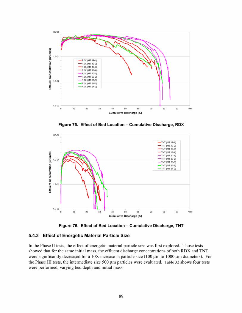
89
1.E-03
1.E-02
1.E-01
1.E+00
0 10 20 30 40 50 60 70 80 90 100
Cumulative Discharge (%)
Efflu
ent C
once
ntra
tion
(C/C
max
)
RDX (MT 19-1)RDX (MT 19-2)RDX (MT 19-3)RDX (MT 19-4)RDX (MT 20-1)RDX (MT 20-2)RDX (MT 20-3)RDX (MT 21-1)RDX (MT 21-2)
Figure 75. Effect of Bed Location – Cumulative Discharge, RDX
1.E-03
1.E-02
1.E-01
1.E+00
0 10 20 30 40 50 60 70 80 90 100
Cumulative Discharge (%)
Efflu
ent C
once
ntra
tion
(C/C
max
)
TNT (MT 19-1)TNT (MT 19-2)TNT (MT 19-3)TNT (MT 19-4)TNT (MT 20-1)TNT (MT 20-2)TNT (MT 20-3)TNT (MT 21-1)TNT (MT 21-2)
Figure 76. Effect of Bed Location – Cumulative Discharge, TNT
5.4.3 Effect of Energetic Material Particle Size
In the Phase II tests, the effect of energetic material particle size was first explored. Those tests showed that for the same initial mass, the effluent discharge concentrations of both RDX and TNT were significantly decreased for a 10X increase in particle size (100 μm to 1000 μm diameters). For the Phase III tests, the intermediate size 500 μm particles were evaluated. Table 32 shows four tests were performed, varying bed depth and initial mass.
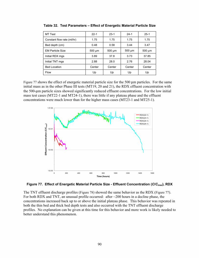
90
Table 32. Test Parameters – Effect of Energetic Material Particle Size
MT Test 22-1 23-1 24-1 25-1
Constant flow rate (ml/hr) 1.75 1.75 1.75 1.75
Bed depth (cm) 0.48 0.58 3.44 3.47
EM Particle Size 500 μm 500 μm 500 μm 500 μm
Initial RDX mgs 3.89 37.8 3.73 37.85
Initial TNT mgs 2.88 28.0 2.76 28.04
Bed Location Center Center Center Center
Flow Up Up Up Up
Figure 77 shows the effect of energetic material particle size for the 500 μm particles. For the same initial mass as in the other Phase III tests (MT19, 20 and 21), the RDX effluent concentration with the 500-μm particle sizes showed significantly reduced effluent concentrations. For the low initial mass test cases (MT22-1 and MT24-1), there was little if any plateau phase and the effluent concentrations were much lower than for the higher mass cases (MT23-1 and MT25-1).
1.E-03
1.E-02
1.E-01
1.E+00
0 200 400 600 800 1000 1200 1400 1600
Time (hours)
Efflu
ent C
once
ntra
iton
(C/C
max
)
RDX(22-1)RDX(23-1)RDX(24-1)RDX(25-1)
Figure 77. Effect of Energetic Material Particle Size - Effluent Concentration (C/Cmax), RDX
The TNT effluent discharge profiles (Figure 78) showed the same behavior as the RDX (Figure 77). For both RDX and TNT, an unusual profile occurred: after ~200 hours in a decline phase, the concentrations increased back up to or above the initial plateau phase. This behavior was repeated in both the thin bed and thick bed depth tests and also occurred with the TNT effluent discharge profiles. No explanation can be given at this time for this behavior and more work is likely needed to better understand this phenomenon.
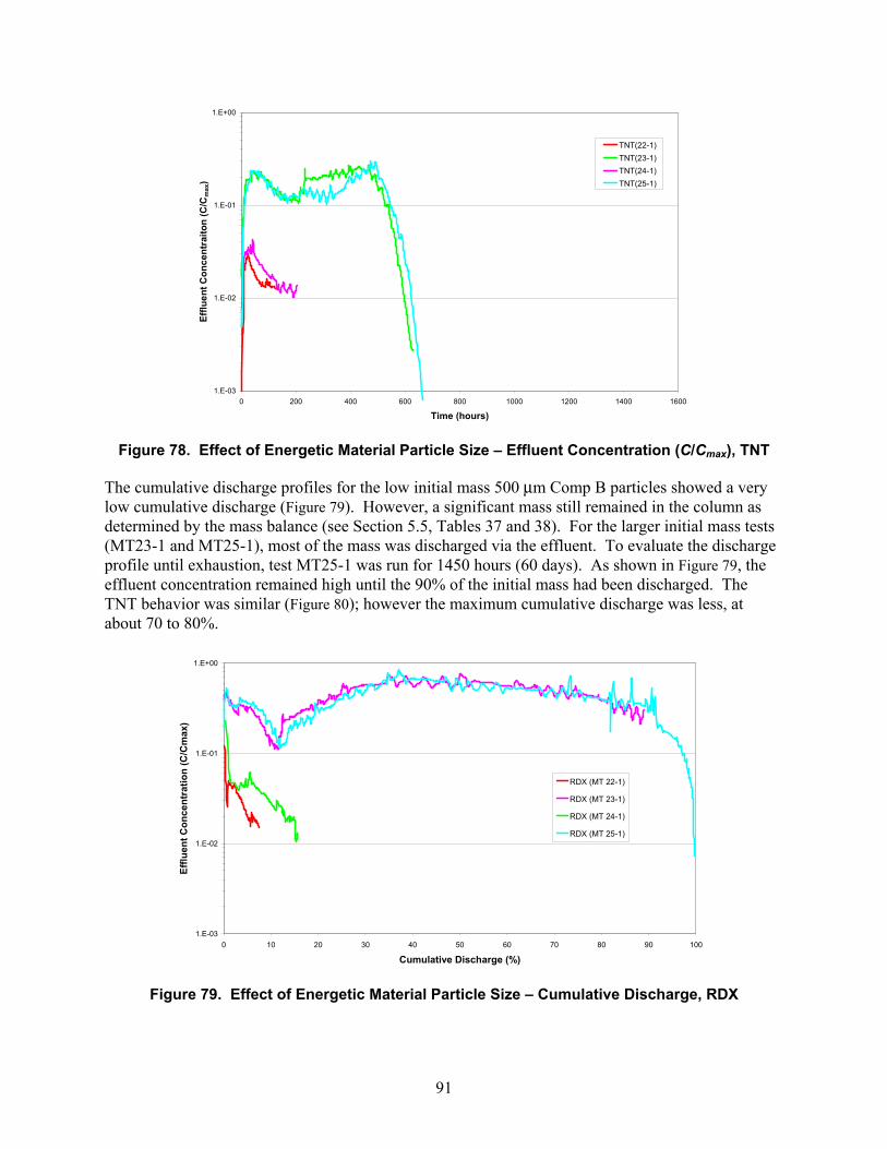
91
1.E-03
1.E-02
1.E-01
1.E+00
0 200 400 600 800 1000 1200 1400 1600
Time (hours)
Efflu
ent C
once
ntra
iton
(C/C
max
)
TNT(22-1)TNT(23-1)TNT(24-1)TNT(25-1)
Figure 78. Effect of Energetic Material Particle Size – Effluent Concentration (C/Cmax), TNT
The cumulative discharge profiles for the low initial mass 500 μm Comp B particles showed a very low cumulative discharge (Figure 79). However, a significant mass still remained in the column as determined by the mass balance (see Section 5.5, Tables 37 and 38). For the larger initial mass tests (MT23-1 and MT25-1), most of the mass was discharged via the effluent. To evaluate the discharge profile until exhaustion, test MT25-1 was run for 1450 hours (60 days). As shown in Figure 79, the effluent concentration remained high until the 90% of the initial mass had been discharged. The TNT behavior was similar (Figure 80); however the maximum cumulative discharge was less, at about 70 to 80%.
1.E-03
1.E-02
1.E-01
1.E+00
0 10 20 30 40 50 60 70 80 90 100
Cumulative Discharge (%)
Efflu
ent C
once
ntra
tion
(C/C
max
)
RDX (MT 22-1)
RDX (MT 23-1)
RDX (MT 24-1)
RDX (MT 25-1)
Figure 79. Effect of Energetic Material Particle Size – Cumulative Discharge, RDX
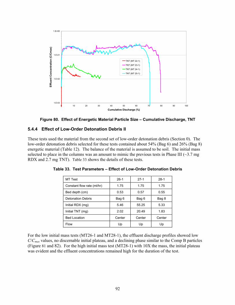
92
1.E-03
1.E-02
1.E-01
1.E+00
0 10 20 30 40 50 60 70 80 90 100
Cumulative Discharge (%)
Efflu
ent C
once
ntra
tion
(C/C
max
)
TNT (MT 22-1)
TNT (MT 23-1)
TNT (MT 24-1)
TNT (MT 25-1)
Figure 80. Effect of Energetic Material Particle Size – Cumulative Discharge, TNT
5.4.4 Effect of Low-Order Detonation Debris II
These tests used the material from the second set of low-order detonation debris (Section 0). The low-order detonation debris selected for these tests contained about 54% (Bag 6) and 26% (Bag 8) energetic material (Table 12). The balance of the material is assumed to be soil. The initial mass selected to place in the columns was an amount to mimic the previous tests in Phase III (~3.7 mg RDX and 2.7 mg TNT). Table 33 shows the details of these tests.
Table 33. Test Parameters – Effect of Low-Order Detonation Debris
MT Test 26-1 27-1 28-1
Constant flow rate (ml/hr) 1.75 1.75 1.75
Bed depth (cm) 0.53 0.57 0.55
Detonation Debris Bag 6 Bag 6 Bag 8
Initial RDX (mg) 5.46 55.25 5.33
Initial TNT (mg) 2.02 20.49 1.83
Bed Location Center Center Center
Flow Up Up Up
For the low initial mass tests (MT26-1 and MT28-1), the effluent discharge profiles showed low C/Cmax values, no discernable initial plateau, and a declining phase similar to the Comp B particles (Figure 81 and 82). For the high initial mass test (MT28-1) with 10X the mass, the initial plateau was evident and the effluent concentrations remained high for the duration of the test.
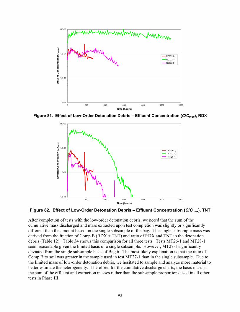
93
1.E-03
1.E-02
1.E-01
1.E+00
0 200 400 600 800 1000 1200
Time (hours)
Efflu
ent C
once
ntra
iton
(C/C
max
)RDX(26-1)RDX(27-1)RDX(28-1)
Figure 81. Effect of Low-Order Detonation Debris – Effluent Concentration (C/Cmax), RDX
1.E-03
1.E-02
1.E-01
1.E+00
0 200 400 600 800 1000 1200
Time (hours)
Efflu
ent C
once
ntra
iton
(C/C
max
)
TNT(26-1)TNT(27-1)TNT(28-1)
Figure 82. Effect of Low-Order Detonation Debris – Effluent Concentration (C/Cmax), TNT
After completion of tests with the low-order detonation debris, we noted that the sum of the cumulative mass discharged and mass extracted upon test completion was slightly or significantly different than the amount based on the single subsample of the bag. The single subsample mass was derived from the fraction of Comp B (RDX + TNT) and ratio of RDX and TNT in the detonation debris (Table 12). Table 34 shows this comparison for all three tests. Tests MT26-1 and MT28-1 seem reasonable given the limited basis of a single subsample. However, MT27-1 significantly deviated from the single subsample basis of Bag 6. The most likely explanation is that the ratio of Comp B to soil was greater in the sample used in test MT27-1 than in the single subsample. Due to the limited mass of low-order detonation debris, we hesitated to sample and analyze more material to better estimate the heterogeneity. Therefore, for the cumulative discharge charts, the basis mass is the sum of the effluent and extraction masses rather than the subsample proportions used in all other tests in Phase III.
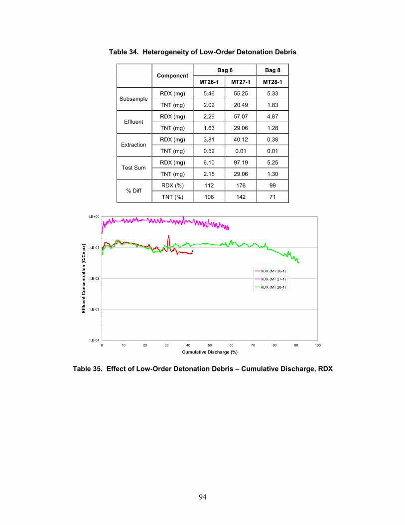
94
Table 34. Heterogeneity of Low-Order Detonation Debris
Bag 6 Bag 8 Component
MT26-1 MT27-1 MT28-1
RDX (mg) 5.46 55.25 5.33 Subsample
TNT (mg) 2.02 20.49 1.83
RDX (mg) 2.29 57.07 4.87 Effluent
TNT (mg) 1.63 29.06 1.28
RDX (mg) 3.81 40.12 0.38 Extraction
TNT (mg) 0.52 0.01 0.01
RDX (mg) 6.10 97.19 5.25 Test Sum
TNT (mg) 2.15 29.06 1.30
RDX (%) 112 176 99 % Diff
TNT (%) 106 142 71
1.E-04
1.E-03
1.E-02
1.E-01
1.E+00
0 10 20 30 40 50 60 70 80 90 100
Cumulative Discharge (%)
Efflu
ent C
once
ntra
tion
(C/C
max
)
RDX (MT 26-1)
RDX (MT 27-1)
RDX (MT 28-1)
Table 35. Effect of Low-Order Detonation Debris – Cumulative Discharge, RDX
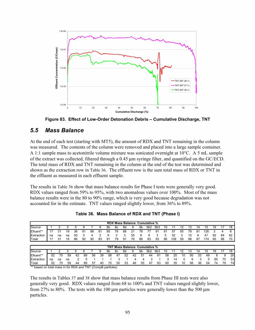
95
1.E-04
1.E-03
1.E-02
1.E-01
1.E+00
0 10 20 30 40 50 60 70 80 90 100
Cumulative Discharge (%)
Efflu
ent C
once
ntra
tion
(C/C
max
)
TNT (MT 26-1)
TNT (MT 27-1)
TNT (MT 28-1)
Figure 83. Effect of Low-Order Detonation Debris – Cumulative Discharge, TNT
5.5 Mass Balance
At the end of each test (starting with MT5), the amount of RDX and TNT remaining in the column was measured. The contents of the column were removed and placed into a large sample container. A 1:1 sample mass to acetonitrile volume mixture was sonicated overnight at 10°C. A 5 mL sample of the extract was collected, filtered through a 0.45 μm syringe filter, and quantified on the GC/ECD. The total mass of RDX and TNT remaining in the column at the end of the test was determined and shown as the extraction row in Table 36. The effluent row is the sum total mass of RDX or TNT in the effluent as measured in each effluent sample. The results in Table 36 show that mass balance results for Phase I tests were generally very good. RDX values ranged from 59% to 95%, with two anomalous values over 100%. Most of the mass balance results were in the 80 to 90% range, which is very good because degradation was not accounted for in the estimate. TNT values ranged slightly lower, from 36% to 89%.
Table 36. Mass Balance of RDX and TNT (Phase I)
Source 1 2 3 5 6 7 8 8b 8c 8d 9 9b 9b2 9b3 10 11 12 13 14 15 16 17 18Efluent** 17 31 19 36 91 88 81 85 76 88 21 78 77 91 91 57 55 78 81 126 3 4 8Extraction na na na 50 0 4 2 6 3 3 55 8 6 3 5 52 3 10 6 47 92 84 62Total 17 31 19 86 92 92 83 91 79 91 76 86 83 93 96 109 59 88 87 174 95 88 70
Source 1 2 3 5 6 7 8 8b 8c 8d 9 9b 9b2 9b3 10 11 12 13 14 15 16 17 18Efluent** 52 75 59 42 89 56 39 68 47 52 42 51 44 61 58 20 10 50 33 49 8 9 20Extraction na na na 2 0 1 1 1 3 1 4 4 3 1 3 14 0 6 3 5 65 70 53Total 52 75 59 44 89 57 40 70 50 53 46 55 47 63 60 35 10 56 36 54 74 79 74** based on total mass in for RDX and TNT (CompB particles)
RDX Mass Balance: Cumulative %
TNT Mass Balance: Cumulative %
The results in Tables 37 and 38 show that mass balance results from Phase III tests were also generally very good. RDX values ranged from 68 to 100% and TNT values ranged slightly lower, from 27% to 80%. The tests with the 100 μm particles were generally lower than the 500 μm particles.
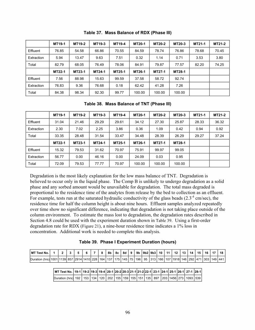
96
Table 37. Mass Balance of RDX (Phase III)
MT19-1 MT19-2 MT19-3 MT19-4 MT20-1 MT20-2 MT20-3 MT21-1 MT21-2
Effluent 76.85 54.58 66.86 70.55 84.59 78.74 76.86 78.68 70.45
Extraction 5.94 13.47 9.63 7.51 0.32 1.14 0.71 3.53 3.80
Total 82.79 68.05 76.49 78.06 84.91 79.87 77.57 82.20 74.25
MT22-1 MT23-1 MT24-1 MT25-1 MT26-1 MT27-1 MT28-1
Effluent 7.56 88.98 15.63 99.59 37.58 58.72 92.74
Extraction 76.83 9.36 76.68 0.18 62.42 41.28 7.26
Total 84.38 98.34 92.30 99.77 100.00 100.00 100.00
Table 38. Mass Balance of TNT (Phase III)
MT19-1 MT19-2 MT19-3 MT19-4 MT20-1 MT20-2 MT20-3 MT21-1 MT21-2
Effluent 31.04 21.46 29.29 29.61 34.12 27.30 25.87 28.33 36.32
Extraction 2.30 7.02 2.25 3.86 0.36 1.09 0.42 0.94 0.92
Total 33.35 28.48 31.54 33.47 34.48 28.39 26.29 29.27 37.24
MT22-1 MT23-1 MT24-1 MT25-1 MT26-1 MT27-1 MT28-1
Effluent 15.32 79.53 31.62 70.97 75.91 99.97 99.05
Extraction 56.77 0.00 46.16 0.00 24.09 0.03 0.95
Total 72.09 79.53 77.77 70.97 100.00 100.00 100.00
Degradation is the most likely explanation for the low mass balance of TNT. Degradation is believed to occur only in the liquid phase. The Comp B is unlikely to undergo degradation as a solid phase and any sorbed amount would be unavailable for degradation. The total mass degraded is proportional to the residence time of the analytes from release by the bed to collection as an effluent. For example, tests run at the saturated hydraulic conductivity of the glass beads (2.3-4 cm/sec), the residence time for half the column height is about nine hours. Effluent samples analyzed repeatedly over time show no significant difference, indicating that degradation is not taking place outside of the column environment. To estimate the mass lost to degradation, the degradation rates described in Section 4.8 could be used with the experiment duration shown in Table 39. Using a first-order degradation rate for RDX (Figure 21), a nine-hour residence time indicates a 1% loss in concentration. Additional work is needed to complete this analysis.
Table 39. Phase I Experiment Duration (hours)
MT Test No. 1 2 3 5 6 7 8 8b 8c 8d 9 9b 9b2 9b3 10 11 12 13 14 15 16 17 18
Duration (hrs) 1001 1139 857 2914 1410 228 164 137 175 145 75 196 95 313 166 107 1918 146 292 471 303 149 441
MT Test No. 19-1 19-2 19-3 19-4 20-1 20-2 20-3 21-1 21-2 22-1 23-1 24-1 25-1 26-1 27-1 28-1
Duration (hrs) 192 153 134 120 202 155 159 155 151 135 897 203 1456 273 1093 539
97
6. Model Development In order to simulate the mass transfer tests, modifications were made to the T2TNT code (Webb et al. 1999). T2TNT is a version of the TOUGH2 code (Pruess 1991) that was modified to include the effects of weather conditions on subsurface conditions as well as the transport of chemicals such as TNT. For this application, a separate solid phase and mass transfer from the solid phase to water were added to the code. The details of the mass transfer model are discussed below. 6.1 Mass Transfer Formulation
The mass transfer rate from a solid to the surrounding fluid is given by:
( )CCSAkm sfi −= ρl
. [9]
where m& is the mass transfer rate from the solid to the liquid phase (kg/s), k is the mass transfer coefficient (m/s), Ai is the solid phase interfacial area (m2),
lS is the liquid saturation, ρf is the fluid density (kg/m3), C is the concentration of the solid material in the far-field fluid (mass fraction), and Cs is the saturation concentration of the solid material in the fluid (mass fraction). In equation [9], the mass transfer from the solid mass to the liquid phase is calculated. The liquid saturation, lS , is included to account for the wetted solid surface area. The mass transfer coefficient, k, and the interfacial area, Ai, are unknowns in the above equation. For the purposes of this initial study, the mass transfer coefficient is assumed to be constant during the modeling of any specific test. Any variation of the mass transfer coefficient with parameters, such as flow rate, could be developed from test series that specifically vary this parameter. The interfacial area, Ai, varies dramatically over time as the mass is transferred from the solid phase into the water phase. The interfacial area is assumed to be a direct function of the time-dependent mass of the solid particles raised to an exponent X, or: X
i MaA = [10]
where a is a constant (m2/kgX), M is the mass of the solid particles (kg), and X is the exponent on the solid mass. The constant a is determined using the initial solid mass and the initial surface area, which is based on initially spherical particles. Using the definition of the interfacial area, the mass transfer relationship can then be written as:
( )CCSMakm sfX −= ρl
.
[11]
98
The fitting parameters for any given simulation run are the mass transfer coefficient, k, and the exponent X. The mass transfer model presented here is intentionally kept simple to easily vary k and X parameters to fit the experimental data and to determine their influence on this fit. In general, the exponent X is a measure of the variation of surface area with mass. For instance, for spherical particles, X is simply 2/3; for long cylinders, X becomes 0.5 where the length is constant (Powers et al. 1994). If the surface changes from smooth to rough (e.g., pitted), the exponent may be less than 0.5. Similarly, if the surface starts out rough and becomes smooth, the exponent may be greater than 1.0. The exponent X may also implicitly include the effect of particle mass and particle size on the mass transfer coefficient, such as the Reynolds number effect, because the mass transfer coefficient, k, is assumed to be constant for each experiment during this initial model development. 6.2 Simulation Model
For the saturated flow tests, two simulation models were developed for the initial data-model comparisons. Both models are one-dimensional. The two models only differ in the bed height of the energetic material. As discussed in Section 4.6, there are two distinct ranges of bed heights, which are between 0.52 and 0.57 cm and between 2.62 and 2.83 cm. For simplicity, only two different bed depths were considered: a nominal 0.5 cm bed depth and a nominal 2.75 cm bed depth. Model meshes were developed for nominal bed depths of 0.5 cm and 2.75 cm as shown in Figure 84. The bed is placed vertically in the center of model. For the 0.5 cm bed height model, the computational domain is discretized using 26 elements with the bed including four of the elements. For the experiments with the 2.75 cm bed depth, the domain is discretized into 55 elements with 20 of the elements comprising the bed. For the pulsed test, which is an unsaturated flow experiment, a different mesh than those for the saturated flow tests was developed because the column dimensions were different. The bed depth in the experiment was 0.49 cm, which was rounded off to 0.5 cm for the model. This mesh is shown in Figure 85. The computational domain is 59 elements total, with 10 elements in the bed. The individual elements in the energetic material bed are not shown due to their small size relative to the total model domain. In this model development phase, only dissolution of RDX is considered.
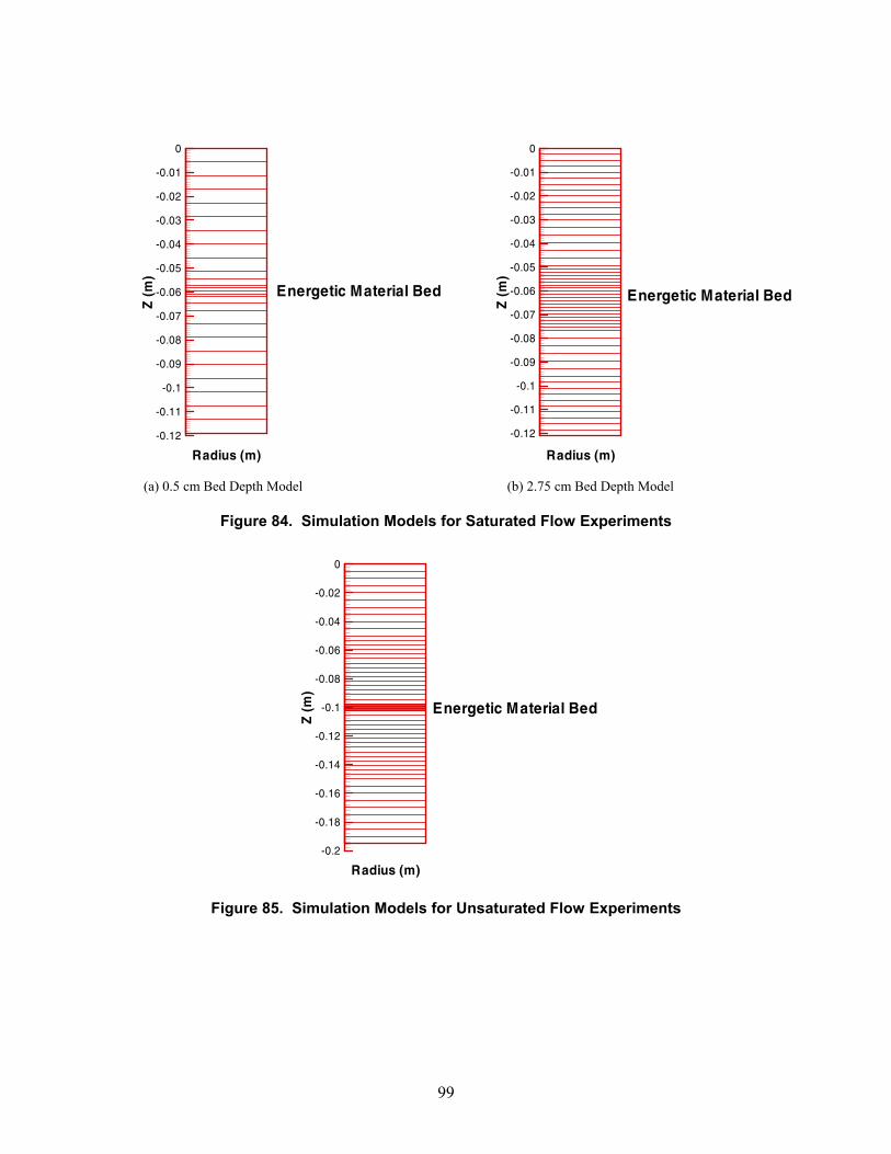
99
Radius (m)
Z(m
)
-0.12
-0.11
-0.1
-0.09
-0.08
-0.07
-0.06
-0.05
-0.04
-0.03
-0.02
-0.01
0
Energetic Material Bed
Radius (m)
Z(m
)
-0.12
-0.11
-0.1
-0.09
-0.08
-0.07
-0.06
-0.05
-0.04
-0.03
-0.02
-0.01
0
Energetic Material Bed
(a) 0.5 cm Bed Depth Model (b) 2.75 cm Bed Depth Model
Figure 84. Simulation Models for Saturated Flow Experiments
Radius (m)
Z(m
)
-0.2
-0.18
-0.16
-0.14
-0.12
-0.1
-0.08
-0.06
-0.04
-0.02
0
Energetic Material Bed
Figure 85. Simulation Models for Unsaturated Flow Experiments
100
6.3 Simulation Parameters
6.3.1 Parameter Definitions
The following simulation parameters were used:
• Diffusion and dispersion • Characteristic curves • Liquid-solid sorption
Diffusion and Dispersion. For simplicity, hydrodynamic dispersion is neglected in the present analysis. Note that the order of magnitude analysis conducted by Imhoff et al. (1993) showed that dispersion is negligible in similar column tests. The energetic material is assumed to exist only as a separate solid phase and in the liquid phase. Molecular diffusion in the liquid phase is calculated using: lll ,0 )( mDD ττφ= [12]
where Dl (m2/sec) is the diffusion coefficient in the liquid phase (Rosenblatt 1991), φ is the porosity,
3/103/10 ll Sφττ = is the saturation-dependent tortuosity model of Millington and Quirk (1961), and
Dm,l (m2/sec) is the molecular diffusion coefficient in liquid. Characteristic Curves. The capillary pressure and relative permeability of the porous media (i.e., the glass beads) is modeled using the standard model of van Genuchten (1980) and Mualem (1976), respectively:
( )[ ] nmecc Sp
/1/1 11 −−= −
α [13]
( )[ ]2/111 mmekekrl SSk −−= [14]
( ) [ ] mmekekrg SSk 2/13/1 11 −−= [15]
where pc (Pa) is the capillary pressure, krl and krg are the liquid relative permeabilities of the liquid and gas phases, respectively, the parameter 1/α (Pa) is approximately the gas entry pressure, and n and m are pore-size distribution parameters. The effective saturation for the capillary pressure, Sec, and relative permeability, Sek, are defined as:
lrc
lrclec S
SSS−−=
1 [16]
grlrk
lrklek SS
SSS−−
−=1
[17]
101
where Sl is the liquid saturation, Slrc and Slrk are the liquid residual saturation for the capillary pressure and relative permeability, respectively, and Sgr is the residual gas pressure. Note that the capillary pressure and relative permeability models are only important in the unsaturated pulse test and during the initial wet-up phase of the saturated flow tests. Liquid-Solid Sorption. Liquid-solid sorption is included in the simulation through specification of a Kd factor, which is the ratio of the concentration on the solid phase, Cs, divided by the concentration in the liquid phase, Cl, or
l
sd C
CK = [18]
and Kd has units of mL/g. 6.3.2 Assigned Values for Simulation Parameters
Generic simulation parameters for all simulations are listed in Table 40. The characteristic curve parameters used in this simulation model have been measured for the glass bead bed as discussed in Section 4.5.
Table 40. Simulation Parameters
Porosity, φ (-) 0.3
Intrinsic permeability, K (m2) 2.4x10⁻¹¹
RDX molecular diffusivity, Dm (m2/sec) 7.15x10⁻¹⁰
n (-) 19.9
m (-) 0.05
1/α (Pa) 10,873.0
Slrc=Slrk (-) 0
Sgr (-) 0.01
For a given saturated flow test, the simulations mimic the various stages of the experiment. Starting from an initially dry column, the wetting-up stage is modeled for approximately 18 to 20 hours. After the wetting-up stage, the water flow rate is essentially constant and is based on actual measurements. As the water flows through the bed in the column, RDX mass is transferred from the solid phase to the water, which subsequently flows through the porous media (glass beads) and finally out of the column. The exit RDX concentration as a function of time from the simulations is then compared to the experimental results, and various parameters (k, X, Kd) are modified to improve the simulation results. Generally, the liquid-solid sorption coefficient, Kd, is kept constant or only varied slightly. The mass transfer coefficient, k, and the surface area exponent, X, are changed to improve the model response compared to the experimental data.

102
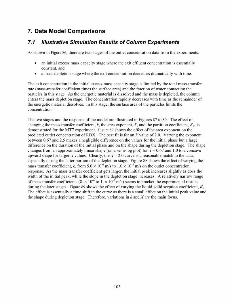
103
7. Data Model Comparisons
7.1 Illustrative Simulation Results of Column Experiments
As shown in Figure 86, there are two stages of the outlet concentration data from the experiments:
• an initial excess mass capacity stage where the exit effluent concentration is essentially constant, and
• a mass depletion stage where the exit concentration decreases dramatically with time. The exit concentration in the initial excess-mass capacity stage is limited by the total mass-transfer rate (mass-transfer coefficient times the surface area) and the fraction of water contacting the particles in this stage. As the energetic material is dissolved and the mass is depleted, the column enters the mass depletion stage. The concentration rapidly decreases with time as the remainder of the energetic material dissolves. In this stage, the surface area of the particles limits the concentration. The two stages and the response of the model are illustrated in Figures 87 to 89. The effect of changing the mass transfer coefficient, k, the area exponent, X, and the partition coefficient, Kd, is demonstrated for the MT7 experiment. Figure 87 shows the effect of the area exponent on the predicted outlet concentration of RDX. The best fit is for an X value of 2.0. Varying the exponent between 0.67 and 2.5 makes a negligible difference on the values for the initial phase but a large difference on the duration of the initial phase and on the shape during the depletion stage. The shape changes from an approximately linear shape (on a semi-log plot) for X = 0.67 and 1.0 to a concave upward shape for larger X values. Clearly, the X = 2.0 curve is a reasonable match to the data, especially during the latter portion of the depletion stage. Figure 88 shows the effect of varying the mass transfer coefficient, k, from 5.0 × 10⁻⁶ m/s to 1.0 × 10⁻⁵ m/s on the outlet concentration response. As the mass transfer coefficient gets larger, the initial peak increases slightly as does the width of the initial peak, while the slope in the depletion stage increases. A relatively narrow range of mass transfer coefficients (8. × 10-6 to 1. × 10-5 m/s) seems to bracket the experimental results during the later stages. Figure 89 shows the effect of varying the liquid-solid sorption coefficient, Kd. The effect is essentially a time shift in the curve as there is a small effect on the initial peak value and the shape during depletion stage. Therefore, variations in k and X are the main focus.
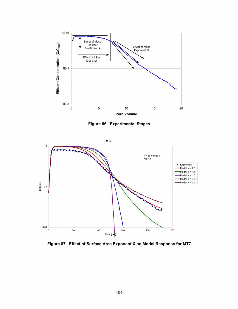
104
1E-2
1E-1
1E+0
0 5 10 15 20
Pore Volume
Efflu
ent C
once
ntra
tion
(C/C
max
) Effect of Mass Transfer
Coefficient, k
Effect of Initial Mass, Mi
Effect of Mass Exponent, X
Figure 86. Experimental Stages
MT7
0.01
0.1
1
0 50 100 150 200 250
Time [hrs]
C/C
max
ExperimentModel: x = 2.0Model: x = 1.5Model: x = 1.0Model: x = 0.67Model: x = 2.5
k = 8e-6 m/secKd = 0
Figure 87. Effect of Surface Area Exponent X on Model Response for MT7
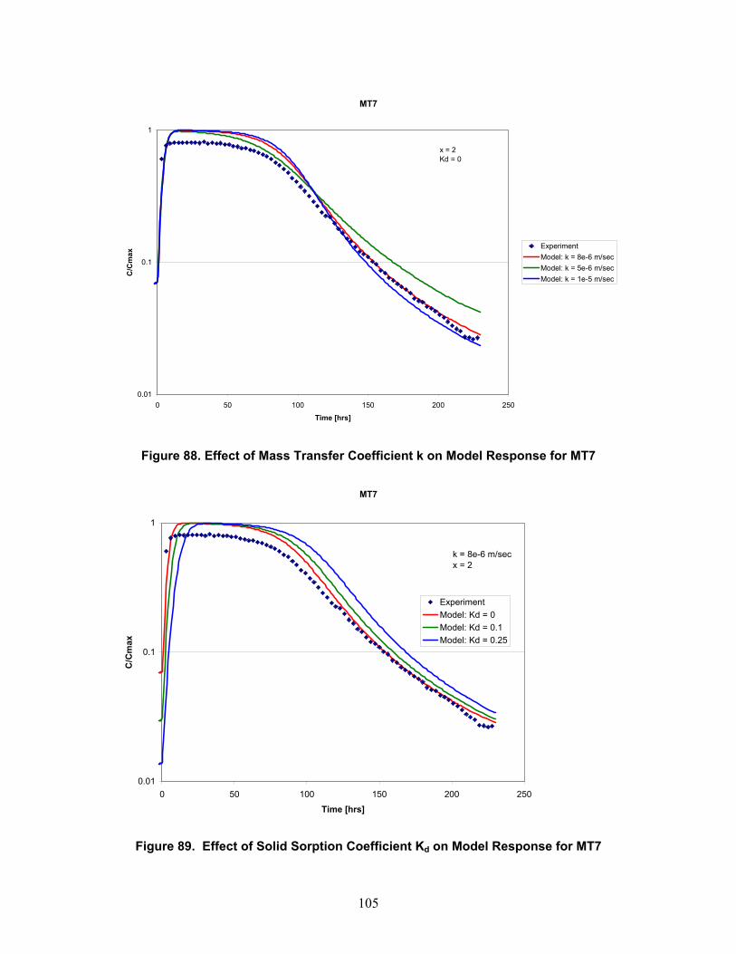
105
MT7
0.01
0.1
1
0 50 100 150 200 250
Time [hrs]
C/C
max
ExperimentModel: k = 8e-6 m/secModel: k = 5e-6 m/secModel: k = 1e-5 m/sec
x = 2Kd = 0
Figure 88. Effect of Mass Transfer Coefficient k on Model Response for MT7
MT7
0.01
0.1
1
0 50 100 150 200 250
Time [hrs]
C/C
max
ExperimentModel: Kd = 0Model: Kd = 0.1Model: Kd = 0.25
k = 8e-6 m/secx = 2
Figure 89. Effect of Solid Sorption Coefficient Kd on Model Response for MT7
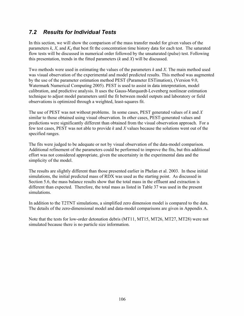
106
7.2 Results for Individual Tests
In this section, we will show the comparison of the mass transfer model for given values of the parameters k, X, and Kd that best fit the concentration time history data for each test. The saturated flow tests will be discussed in numerical order followed by the unsaturated (pulse) test. Following this presentation, trends in the fitted parameters (k and X) will be discussed. Two methods were used in estimating the values of the parameters k and X. The main method used was visual observation of the experimental and model predicted results. This method was augmented by the use of the parameter estimation method PEST (Parameter ESTimation), (Version 9.0, Watermark Numerical Computing 2005). PEST is used to assist in data interpretation, model calibration, and predictive analysis. It uses the Gauss-Marquardt-Levenberg nonlinear estimation technique to adjust model parameters until the fit between model outputs and laboratory or field observations is optimized through a weighted, least-squares fit. The use of PEST was not without problems. In some cases, PEST generated values of k and X similar to those obtained using visual observation. In other cases, PEST-generated values and predictions were significantly different than obtained from the visual observation approach. For a few test cases, PEST was not able to provide k and X values because the solutions went out of the specified ranges. The fits were judged to be adequate or not by visual observation of the data-model comparison. Additional refinement of the parameters could be performed to improve the fits, but this additional effort was not considered appropriate, given the uncertainty in the experimental data and the simplicity of the model. The results are slightly different than those presented earlier in Phelan et al. 2003. In these initial simulations, the initial predicted mass of RDX was used as the starting point. As discussed in Section 5.6, the mass balance results show that the total mass in the effluent and extraction is different than expected. Therefore, the total mass as listed in Table 37 was used in the present simulations. In addition to the T2TNT simulations, a simplified zero dimension model is compared to the data. The details of the zero-dimensional model and data-model comparisons are given in Appendix A. Note that the tests for low-order detonation debris (MT11, MT15, MT26, MT27, MT28) were not simulated because there is no particle size information.
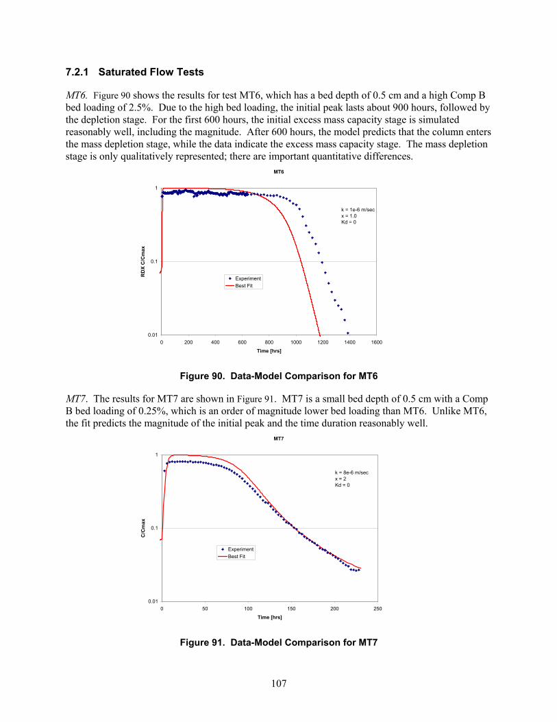
107
7.2.1 Saturated Flow Tests
MT6. Figure 90 shows the results for test MT6, which has a bed depth of 0.5 cm and a high Comp B bed loading of 2.5%. Due to the high bed loading, the initial peak lasts about 900 hours, followed by the depletion stage. For the first 600 hours, the initial excess mass capacity stage is simulated reasonably well, including the magnitude. After 600 hours, the model predicts that the column enters the mass depletion stage, while the data indicate the excess mass capacity stage. The mass depletion stage is only qualitatively represented; there are important quantitative differences.
MT6
0.01
0.1
1
0 200 400 600 800 1000 1200 1400 1600
Time [hrs]
RD
X C
/Cm
ax
ExperimentBest Fit
k = 1e-6 m/secx = 1.0Kd = 0
Figure 90. Data-Model Comparison for MT6
MT7. The results for MT7 are shown in Figure 91. MT7 is a small bed depth of 0.5 cm with a Comp B bed loading of 0.25%, which is an order of magnitude lower bed loading than MT6. Unlike MT6, the fit predicts the magnitude of the initial peak and the time duration reasonably well.
MT7
0.01
0.1
1
0 50 100 150 200 250
Time [hrs]
C/C
max
ExperimentBest Fit
k = 8e-6 m/secx = 2Kd = 0
Figure 91. Data-Model Comparison for MT7
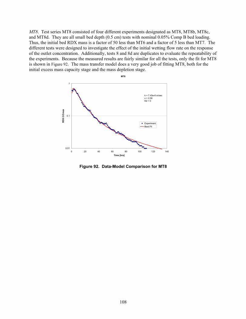
108
MT8. Test series MT8 consisted of four different experiments designated as MT8, MT8b, MT8c, and MT8d. They are all small bed depth (0.5 cm) tests with nominal 0.05% Comp B bed loading. Thus, the initial bed RDX mass is a factor of 50 less than MT6 and a factor of 5 less than MT7. The different tests were designed to investigate the effect of the initial wetting flow rate on the response of the outlet concentration. Additionally, tests 8 and 8d are duplicates to evaluate the repeatability of the experiments. Because the measured results are fairly similar for all the tests, only the fit for MT8 is shown in Figure 92. The mass transfer model does a very good job of fitting MT8, both for the initial excess mass capacity stage and the mass depletion stage.
MT8
0.01
0.1
1
0 20 40 60 80 100 120 140
Time [hrs]
RD
X C
/Cm
ax
ExperimentBest Fit
k = 7.45e-6 m/secx = 2.58Kd = 0
Figure 92. Data-Model Comparison for MT8
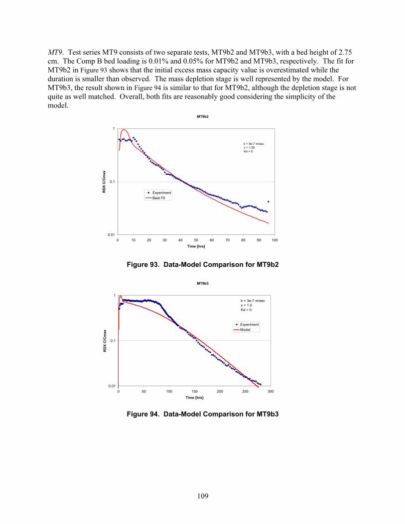
109
MT9. Test series MT9 consists of two separate tests, MT9b2 and MT9b3, with a bed height of 2.75 cm. The Comp B bed loading is 0.01% and 0.05% for MT9b2 and MT9b3, respectively. The fit for MT9b2 in Figure 93 shows that the initial excess mass capacity value is overestimated while the duration is smaller than observed. The mass depletion stage is well represented by the model. For MT9b3, the result shown in Figure 94 is similar to that for MT9b2, although the depletion stage is not quite as well matched. Overall, both fits are reasonably good considering the simplicity of the model.
MT9b2
0.01
0.1
1
0 10 20 30 40 50 60 70 80 90 100
Time [hrs]
RD
X C
/Cm
ax
ExperimentBest Fit
k = 9e-7 m/secx = 1.56Kd = 0
Figure 93. Data-Model Comparison for MT9b2
MT9b3
0.01
0.1
1
0 50 100 150 200 250 300
Time [hrs]
RD
X C
/Cm
ax
ExperimentModel
k = 3e-7 m/secx = 1.0Kd = 0
Figure 94. Data-Model Comparison for MT9b3
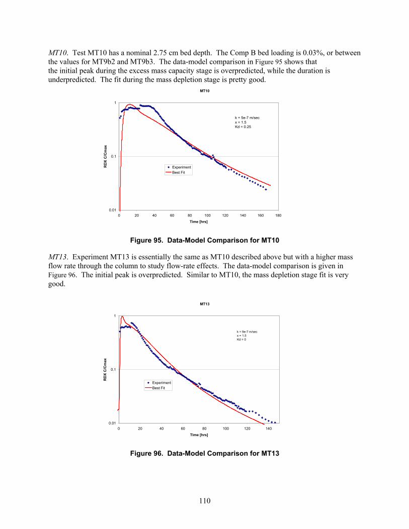
110
MT10. Test MT10 has a nominal 2.75 cm bed depth. The Comp B bed loading is 0.03%, or between the values for MT9b2 and MT9b3. The data-model comparison in Figure 95 shows that the initial peak during the excess mass capacity stage is overpredicted, while the duration is underpredicted. The fit during the mass depletion stage is pretty good.
MT10
0.01
0.1
1
0 20 40 60 80 100 120 140 160 180
Time [hrs]
RD
X C
/Cm
ax
ExperimentBest Fit
k = 5e-7 m/secx = 1.5Kd = 0.25
Figure 95. Data-Model Comparison for MT10
MT13. Experiment MT13 is essentially the same as MT10 described above but with a higher mass flow rate through the column to study flow-rate effects. The data-model comparison is given in Figure 96. The initial peak is overpredicted. Similar to MT10, the mass depletion stage fit is very good.
MT13
0.01
0.1
1
0 20 40 60 80 100 120 140
Time [hrs]
RD
X C
/Cm
ax
ExperimentBest Fit
k = 9e-7 m/secx = 1.5Kd = 0
Figure 96. Data-Model Comparison for MT13
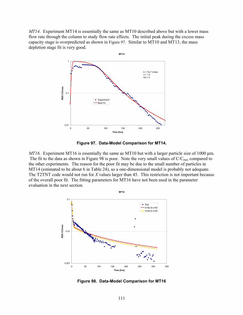
111
MT14. Experiment MT14 is essentially the same as MT10 described above but with a lower mass flow rate through the column to study flow rate effects. The initial peak during the excess mass capacity stage is overpredicted as shown in Figure 97. Similar to MT10 and MT13, the mass depletion stage fit is very good.
MT14
0.01
0.1
1
0 50 100 150 200 250
Time [hrs]
RD
X C
/Cm
ax
ExperimentBest Fit
k = 7e-7 m/secx = 1.5Kd = 0
Figure 97. Data-Model Comparison for MT14.
MT16. Experiment MT16 is essentially the same as MT10 but with a larger particle size of 1000 μm. The fit to the data as shown in Figure 98 is poor. Note the very small values of C/Cmax compared to the other experiments. The reason for the poor fit may be due to the small number of particles in MT14 (estimated to be about 6 in Table 24), so a one-dimensional model is probably not adequate. The T2TNT code would not run for X values larger than 45. This restriction is not important because of the overall poor fit. The fitting parameters for MT16 have not been used in the parameter evaluation in the next section.
MT16
0.001
0.01
0.1
0 50 100 150 200 250 300 350
Time [hrs]
RD
X C
/Cm
ax
Expk=5e-8 x=40k=5e-8 x=45
Figure 98. Data-Model Comparison for MT16
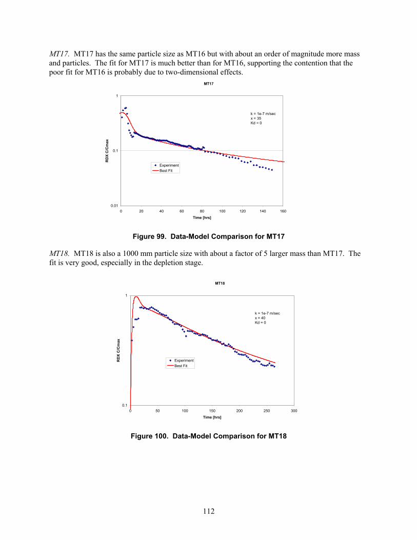
112
MT17. MT17 has the same particle size as MT16 but with about an order of magnitude more mass and particles. The fit for MT17 is much better than for MT16, supporting the contention that the poor fit for MT16 is probably due to two-dimensional effects.
MT17
0.01
0.1
1
0 20 40 60 80 100 120 140 160
Time [hrs]
RD
X C
/Cm
ax
ExperimentBest Fit
k = 1e-7 m/secx = 35Kd = 0
Figure 99. Data-Model Comparison for MT17
MT18. MT18 is also a 1000 mm particle size with about a factor of 5 larger mass than MT17. The fit is very good, especially in the depletion stage.
MT18
0.1
1
0 50 100 150 200 250 300
Time [hrs]
RD
X C
/Cm
ax
ExperimentBest Fit
k = 1e-7 m/secx = 40Kd = 0
Figure 100. Data-Model Comparison for MT18
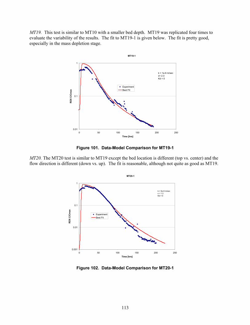
113
MT19. This test is similar to MT10 with a smaller bed depth. MT19 was replicated four times to evaluate the variability of the results. The fit to MT19-1 is given below. The fit is pretty good, especially in the mass depletion stage.
MT19-1
0.01
0.1
1
0 50 100 150 200 250
Time [hrs]
RD
X C
/Cm
ax
ExperimentBest Fit
k = 1e-6 m/secx= 2.3Kd = 0
Figure 101. Data-Model Comparison for MT19-1
MT20. The MT20 test is similar to MT19 except the bed location is different (top vs. center) and the flow direction is different (down vs. up). The fit is reasonable, although not quite as good as MT19.
MT20-1
0.001
0.01
0.1
1
0 50 100 150 200 250
Time [hrs]
RD
X C
/Cm
ax
ExperimentBest Fit
k = 5e-6 m/secx = 1.3Kd = 0
Figure 102. Data-Model Comparison for MT20-1
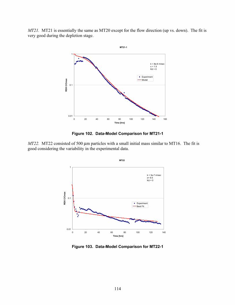
114
MT21. MT21 is essentially the same as MT20 except for the flow direction (up vs. down). The fit is very good during the depletion stage.
MT21-1
0.01
0.1
1
0 20 40 60 80 100 120 140 160
Time [hrs]
RD
X C
/Cm
ax
ExperimentModel
k = 8e-6 m/secx = 1.5Kd = 0
Figure 102. Data-Model Comparison for MT21-1
MT22. MT22 consisted of 500 μm particles with a small initial mass similar to MT16. The fit is good considering the variability in the experimental data.
MT22
0.01
0.1
1
0 20 40 60 80 100 120 140
Time [hrs]
RD
X C
/Cm
ax
ExperimentBest Fit
k = 3e-7 m/secx= 9.5Kd = 0
Figure 103. Data-Model Comparison for MT22-1
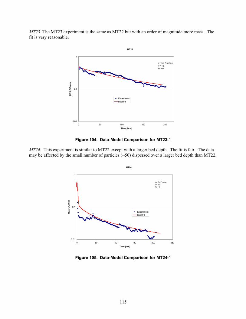
115
MT23. The MT23 experiment is the same as MT22 but with an order of magnitude more mass. The fit is very reasonable.
MT23
0.01
0.1
1
0 50 100 150 200
Time [hrs]
RD
X C
/Cm
ax
ExperimentBest Fit
k = 5e-7 m/secx = 15Kd =0
Figure 104. Data-Model Comparison for MT23-1
MT24. This experiment is similar to MT22 except with a larger bed depth. The fit is fair. The data may be affected by the small number of particles (~50) dispersed over a larger bed depth than MT22.
MT24
0.01
0.1
1
0 50 100 150 200 250
Time [hrs]
RD
X C
/Cm
ax
ExperimentBest Fit
k = 3e-7 m/secx = 9.5Kd = 0
Figure 105. Data-Model Comparison for MT24-1
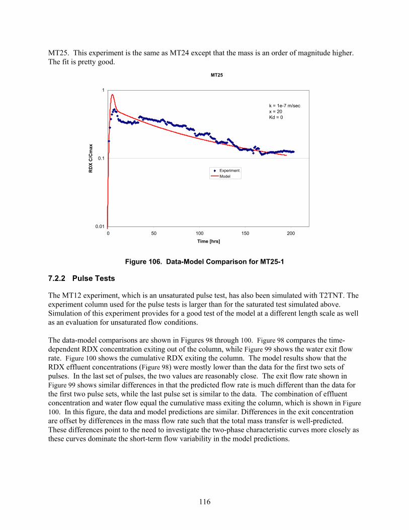
116
MT25. This experiment is the same as MT24 except that the mass is an order of magnitude higher. The fit is pretty good.
MT25
0.01
0.1
1
0 50 100 150 200
Time [hrs]
RD
X C
/Cm
ax
ExperimentModel
k = 1e-7 m/secx = 20Kd = 0
Figure 106. Data-Model Comparison for MT25-1
7.2.2 Pulse Tests
The MT12 experiment, which is an unsaturated pulse test, has also been simulated with T2TNT. The experiment column used for the pulse tests is larger than for the saturated test simulated above. Simulation of this experiment provides for a good test of the model at a different length scale as well as an evaluation for unsaturated flow conditions. The data-model comparisons are shown in Figures 98 through 100. Figure 98 compares the time-dependent RDX concentration exiting out of the column, while Figure 99 shows the water exit flow rate. Figure 100 shows the cumulative RDX exiting the column. The model results show that the RDX effluent concentrations (Figure 98) were mostly lower than the data for the first two sets of pulses. In the last set of pulses, the two values are reasonably close. The exit flow rate shown in Figure 99 shows similar differences in that the predicted flow rate is much different than the data for the first two pulse sets, while the last pulse set is similar to the data. The combination of effluent concentration and water flow equal the cumulative mass exiting the column, which is shown in Figure 100. In this figure, the data and model predictions are similar. Differences in the exit concentration are offset by differences in the mass flow rate such that the total mass transfer is well-predicted. These differences point to the need to investigate the two-phase characteristic curves more closely as these curves dominate the short-term flow variability in the model predictions.
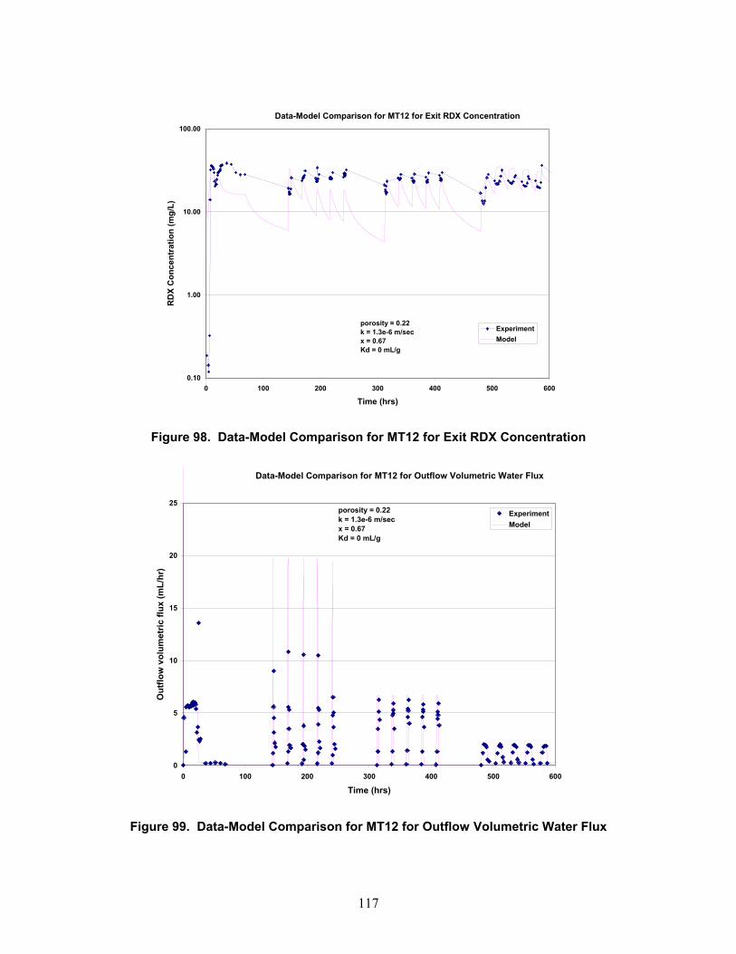
117
Data-Model Comparison for MT12 for Exit RDX Concentration
0.10
1.00
10.00
100.00
0 100 200 300 400 500 600
Time (hrs)
RD
X C
once
ntra
tion
(mg/
L)
ExperimentModel
porosity = 0.22k = 1.3e-6 m/secx = 0.67Kd = 0 mL/g
Figure 98. Data-Model Comparison for MT12 for Exit RDX Concentration
Data-Model Comparison for MT12 for Outflow Volumetric Water Flux
0
5
10
15
20
25
0 100 200 300 400 500 600
Time (hrs)
Out
flow
vol
umet
ric fl
ux (m
L/hr
)
ExperimentModel
porosity = 0.22k = 1.3e-6 m/secx = 0.67Kd = 0 mL/g
Figure 99. Data-Model Comparison for MT12 for Outflow Volumetric Water Flux
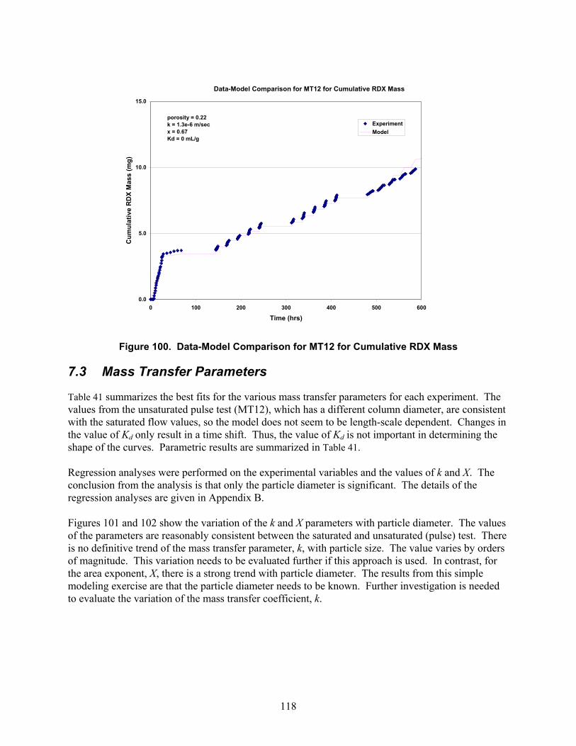
118
Data-Model Comparison for MT12 for Cumulative RDX Mass
0.0
5.0
10.0
15.0
0 100 200 300 400 500 600
Time (hrs)
Cum
ulat
ive
RD
X M
ass
(mg)
ExperimentModel
porosity = 0.22k = 1.3e-6 m/secx = 0.67Kd = 0 mL/g
Figure 100. Data-Model Comparison for MT12 for Cumulative RDX Mass
7.3 Mass Transfer Parameters
Table 41 summarizes the best fits for the various mass transfer parameters for each experiment. The values from the unsaturated pulse test (MT12), which has a different column diameter, are consistent with the saturated flow values, so the model does not seem to be length-scale dependent. Changes in the value of Kd only result in a time shift. Thus, the value of Kd is not important in determining the shape of the curves. Parametric results are summarized in Table 41. Regression analyses were performed on the experimental variables and the values of k and X. The conclusion from the analysis is that only the particle diameter is significant. The details of the regression analyses are given in Appendix B. Figures 101 and 102 show the variation of the k and X parameters with particle diameter. The values of the parameters are reasonably consistent between the saturated and unsaturated (pulse) test. There is no definitive trend of the mass transfer parameter, k, with particle size. The value varies by orders of magnitude. This variation needs to be evaluated further if this approach is used. In contrast, for the area exponent, X, there is a strong trend with particle diameter. The results from this simple modeling exercise are that the particle diameter needs to be known. Further investigation is needed to evaluate the variation of the mass transfer coefficient, k.
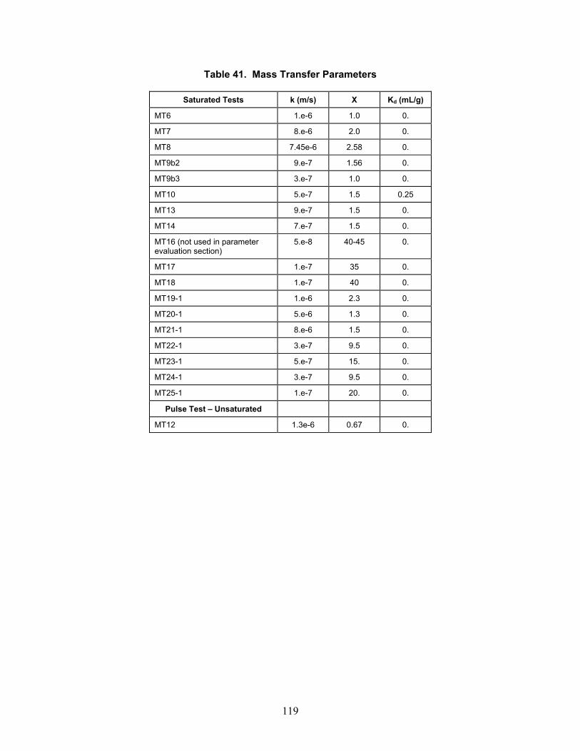
119
Table 41. Mass Transfer Parameters
Saturated Tests k (m/s) X Kd (mL/g)
MT6 1.e-6 1.0 0.
MT7 8.e-6 2.0 0.
MT8 7.45e-6 2.58 0.
MT9b2 9.e-7 1.56 0.
MT9b3 3.e-7 1.0 0.
MT10 5.e-7 1.5 0.25
MT13 9.e-7 1.5 0.
MT14 7.e-7 1.5 0.
MT16 (not used in parameter evaluation section)
5.e-8 40-45 0.
MT17 1.e-7 35 0.
MT18 1.e-7 40 0.
MT19-1 1.e-6 2.3 0.
MT20-1 5.e-6 1.3 0.
MT21-1 8.e-6 1.5 0.
MT22-1 3.e-7 9.5 0.
MT23-1 5.e-7 15. 0.
MT24-1 3.e-7 9.5 0.
MT25-1 1.e-7 20. 0.
Pulse Test – Unsaturated
MT12 1.3e-6 0.67 0.
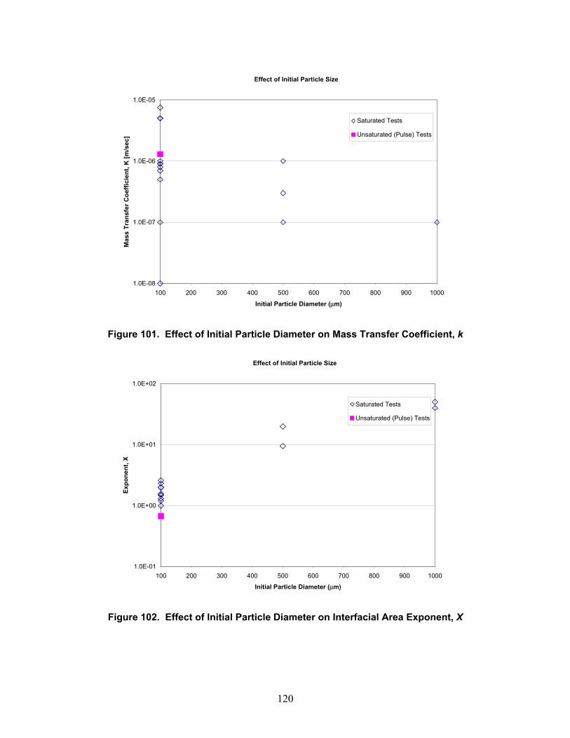
120
Effect of Initial Particle Size
1.0E-08
1.0E-07
1.0E-06
1.0E-05
100 200 300 400 500 600 700 800 900 1000
Initial Particle Diameter (μm)
Mas
s Tr
ansf
er C
oeffi
cien
t, K
[m/s
ec]
Saturated Tests
Unsaturated (Pulse) Tests
Figure 101. Effect of Initial Particle Diameter on Mass Transfer Coefficient, k
Effect of Initial Particle Size
1.0E-01
1.0E+00
1.0E+01
1.0E+02
100 200 300 400 500 600 700 800 900 1000
Initial Particle Diameter (μm)
Expo
nent
, X
Saturated Tests
Unsaturated (Pulse) Tests
Figure 102. Effect of Initial Particle Diameter on Interfacial Area Exponent, X
121
7.4 Discussion
A simple mass transfer formulation has been added to T2TNT to simulate the present experiments for RDX dissolution and transport. The model contains two fitting parameters – the mass transfer coefficient from the solid phase to the water, k, and an exponent on the solid surface area function, X. The parameters are varied to try to match the measured exit RDX concentration as a function of time. There are two general regions in the outlet concentration data – an initial excess mass capacity stage and a mass depletion stage. The mass transfer coefficient, k, was most important in the prediction of the initial stage, while the area parameter X was most important in the depletion stage. A sorption coefficient, Kd, was also included in the model, but it was essentially a time shift parameter that had little influence on the shape of the curve. The parameters were varied for the individual experiments, and most of the fits matched the data reasonably well, especially in the mass depletion stage. Saturated flow and an unsaturated pulse experiment were modeled. The values of k and X were reasonably consistent for the two types of tests (saturated steady-state and unsaturated transient). While the variation of the surface area exponent, X, can be correlated with the initial particle diameter with some degree of success, the variation of the mass transfer parameter, k, has not been successful. Further work on evaluating the influence of various parameters, such as flow rate, on the value of k needs to be performed if the present approach is pursued.

122
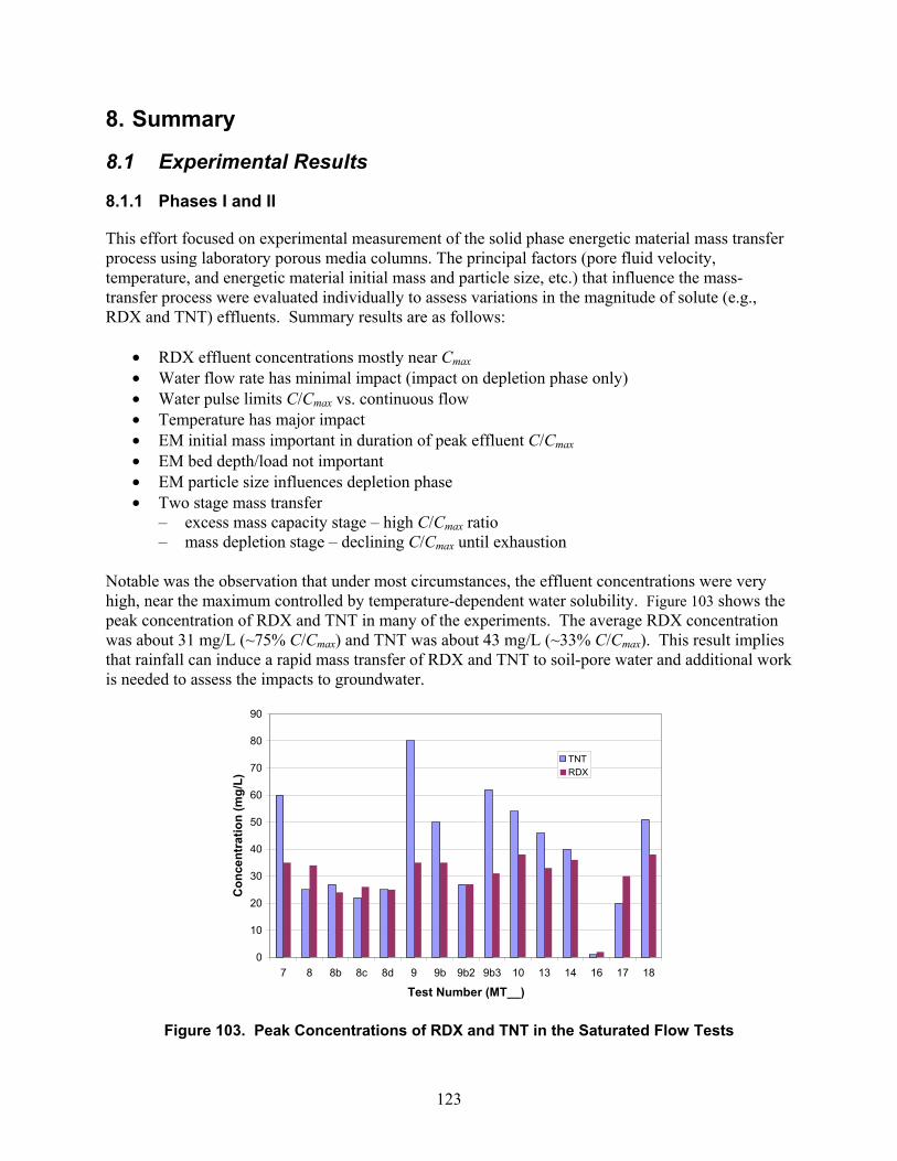
123
8. Summary
8.1 Experimental Results
8.1.1 Phases I and II
This effort focused on experimental measurement of the solid phase energetic material mass transfer process using laboratory porous media columns. The principal factors (pore fluid velocity, temperature, and energetic material initial mass and particle size, etc.) that influence the mass-transfer process were evaluated individually to assess variations in the magnitude of solute (e.g., RDX and TNT) effluents. Summary results are as follows:
• RDX effluent concentrations mostly near Cmax • Water flow rate has minimal impact (impact on depletion phase only) • Water pulse limits C/Cmax vs. continuous flow • Temperature has major impact • EM initial mass important in duration of peak effluent C/Cmax • EM bed depth/load not important • EM particle size influences depletion phase • Two stage mass transfer
– excess mass capacity stage – high C/Cmax ratio – mass depletion stage – declining C/Cmax until exhaustion
Notable was the observation that under most circumstances, the effluent concentrations were very high, near the maximum controlled by temperature-dependent water solubility. Figure 103 shows the peak concentration of RDX and TNT in many of the experiments. The average RDX concentration was about 31 mg/L (~75% C/Cmax) and TNT was about 43 mg/L (~33% C/Cmax). This result implies that rainfall can induce a rapid mass transfer of RDX and TNT to soil-pore water and additional work is needed to assess the impacts to groundwater.
0
10
20
30
40
50
60
70
80
90
7 8 8b 8c 8d 9 9b 9b2 9b3 10 13 14 16 17 18
Test Number (MT__)
Con
cent
ratio
n (m
g/L)
TNTRDX
Figure 103. Peak Concentrations of RDX and TNT in the Saturated Flow Tests
124
8.1.2 Phase III
This effort continued previous experimental measurements of solid-phase energetic material mass-transfer processes using laboratory porous-media columns. The key factors of surface deposits vs. buried deposits, energetic material particle size, and low-order detonation debris were explored. In addition, test replicates were completed to assess experimental variability that will help better understand true differences due to changes in experimental conditions. As in Phases I and II, under most circumstances, the effluent concentrations were very high, near the maximum controlled by temperature-dependent water solubility. Differences in C/Cmax peak levels and duration during the excess mass capacity stage and the slope of the depletion phase continue to provide important features that need to be incorporated in the mass-transfer model. The effect of test replication test series showed that effluent concentration profiles of replicate tests were fairly uniform and that RDX profiles appeared more uniform than the TNT profiles. Plots of the cumulative discharge profiles showed more discrimination of the net mass discharge and also revealed that one test (MT19-2) was significantly lower than the rest. This result provides the reader with a better understanding of normal test variation and provides a guide for comparison with changes in experimental conditions. The effect of bed location showed that in general, surface deposits showed slightly sustained greater effluent concentrations for both RDX and TNT. However, as shown in the cumulative discharge profiles, as the mass became depleted, the effluent concentrations declined more rapidly. The cumulative discharge of RDX showed high values of 70 to 85%; however, TNT values were significantly lower, at 25 to 40%. The remaining mass in the column after test termination showed very small amounts. Thus, degradation losses must account for the difference. The initial mass and total surface area of energetic material particles plays a key role in the effluent concentrations of RDX and TNT. With a similar mass, but a 5X increase in particle diameter, the effluent concentrations never reach peak concentrations as with the smaller particles. Increasing the mass (and the total surface area) with the larger particles creates an effluent profile similar to that with the smaller particles. The low-order detonation debris used in the Phase III tests contained both soil and energetic material. With similar initial-mass buried deposits, the low-order detonation debris showed significantly lower peak effluent concentrations and a slower decline in the mass depletion stages. These effects may be due to partitioning onto the soil solid phase or may be an effect of the detonation on the energetic material. Taylor et al. (2003) describes visual interpretations that some of the low-order detonation debris may have been melted and resolidified upon cooling. Bag 8 (>500 μm) showed a similar effluent concentration profile as the 500 μm particles in MT23-1 and MT25-1. With a 10X increase in initial mass, the effluent concentrations of Bag 6 remained very high, consistent with the Comp B high initial mass test in Phase II (MT17 and MT18).
125
8.2 Modeling
A simple mass transfer formulation has been added to T2TNT to simulate experiments for Comp B dissolution and transport. The model contains two fitting parameters – the mass transfer coefficient from the solid phase to the water, k, and an exponent on the solid surface area function, X. The parameters were varied for the individual experiments and most of the fits match the data reasonably well for both saturated flow and unsaturated pulse experiment. The values of k and X are reasonably consistent for both types of tests (saturated steady state and unsaturated transient). The modeling effort was successful in fitting a simple two-parameter mass transfer function. The experimental design for the laboratory tests was not structured for statistical analysis, which chal-lenged the structured statistical analysis to develop correlations and significance (Appendix B). However, the statistical analysis supports a hypothesis that the variation of the surface area exponent, X, is correlated with the initial particle diameter – the greater the initial particle diameter, the greater the surface area exponent. This has importance principally in the mass depletion stage where small initial particles are exhausted in a narrow time window with a precipitous drop in effluent concentration compared to a much longer and slower decline for larger particles (see Figure 87). This implies that particle size distributions for detonation debris on ranges may be needed for accurate estimates of mass transfer rates into soil over longer time domains that include mass depletion stages. Statistical correlations for the mass transfer parameter, k, did not show any significant relationships with the experimental parameters. However, we observed that the fitted mass transfer coefficients were in a narrow range (for the experimental conditions employed) and may represent a general mass transfer rate that is not dependent on other external conditions. This would benefit applications of the mass transfer function by simplifying input parameters needed for analysis of the pollution potential of various range contamination conditions.

126
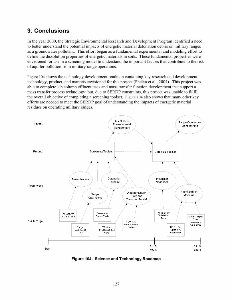
127
9. Conclusions In the year 2000, the Strategic Environmental Research and Development Program identified a need to better understand the potential impacts of energetic material detonation debris on military ranges as a groundwater pollutant. This effort began as a fundamental experimental and modeling effort to define the dissolution properties of energetic materials in soils. These fundamental properties were envisioned for use in a screening model to understand the important factors that contribute to the risk of aquifer pollution from military range operations. Figure 104 shows the technology development roadmap containing key research and development, technology, product, and markets envisioned for this project (Phelan et al., 2004). This project was able to complete lab column effluent tests and mass transfer function development that support a mass transfer process technology; but, due to SERDP constraints, this project was unable to fulfill the overall objective of completing a screening toolset. Figure 104 also shows that many other key efforts are needed to meet the SERDP goal of understanding the impacts of energetic material residues on operating military ranges.
Figure 104. Science and Technology Roadmap
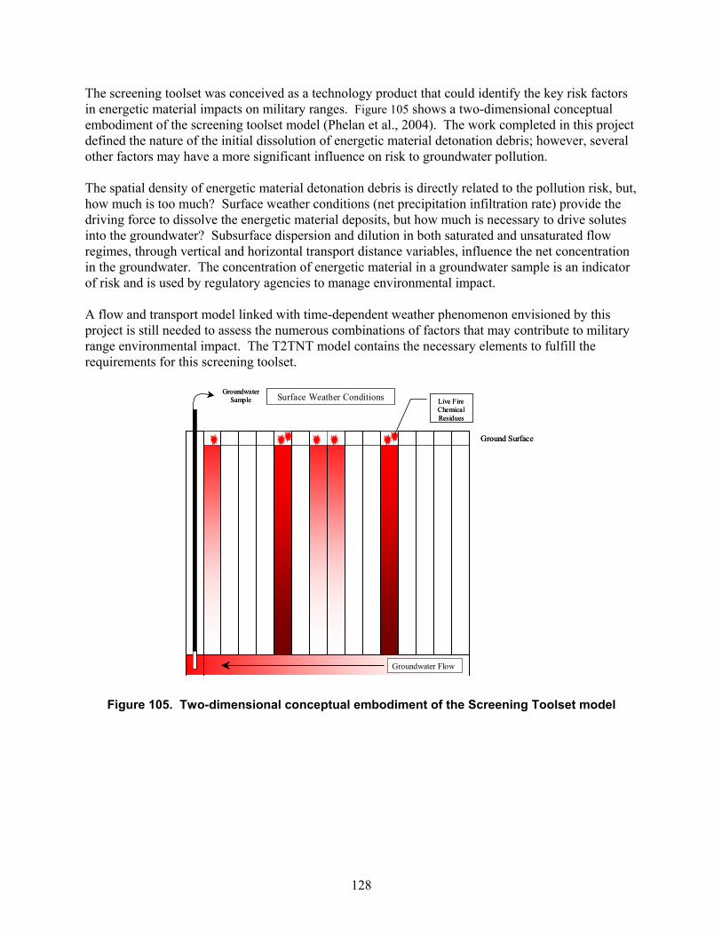
128
The screening toolset was conceived as a technology product that could identify the key risk factors in energetic material impacts on military ranges. Figure 105 shows a two-dimensional conceptual embodiment of the screening toolset model (Phelan et al., 2004). The work completed in this project defined the nature of the initial dissolution of energetic material detonation debris; however, several other factors may have a more significant influence on risk to groundwater pollution. The spatial density of energetic material detonation debris is directly related to the pollution risk, but, how much is too much? Surface weather conditions (net precipitation infiltration rate) provide the driving force to dissolve the energetic material deposits, but how much is necessary to drive solutes into the groundwater? Subsurface dispersion and dilution in both saturated and unsaturated flow regimes, through vertical and horizontal transport distance variables, influence the net concentration in the groundwater. The concentration of energetic material in a groundwater sample is an indicator of risk and is used by regulatory agencies to manage environmental impact. A flow and transport model linked with time-dependent weather phenomenon envisioned by this project is still needed to assess the numerous combinations of factors that may contribute to military range environmental impact. The T2TNT model contains the necessary elements to fulfill the requirements for this screening toolset.
Groundwater Sample Live Fire
Chemical Residues
Groundwater Flow
Surface Weather Conditions
Ground Surface
Groundwater Sample Live Fire
Chemical Residues
Groundwater Flow
Surface Weather Conditions
Ground Surface
Figure 105. Two-dimensional conceptual embodiment of the Screening Toolset model
129
References Andraski, B.J., 1997, “Test-Trench Studies in the Amargosa Desert, Southern Nevada: Results and Application of Information to Landfill Covers in Arid Environments,” Conference Proceedings, Landfill capping in the semi-arid west: Problems, perspectives, and solutions, Environmental Science and Research Foundation, Idaho Falls, ID, pp. 165-179.
Braud, I., Dantas-Antonino, A.C., Vauclin, M., Thony, J.L., Ruelle, P. (1995). “A Simple Soil-Plant-Atmosphere Transfer Model (SiSPAT) Development and Field Verification,” Journal of Hydrology 166:213-250.
Braud, I., J. Noilhan, P. Bessemoulin, P. Mascart, R. Haverkamp, and M. Vauclin, 1993, “Bare-Ground Surface Heat and Water Exchanges Under Dry Conditions: Observations and Parameterization,” Boundary-Layer Meteorology, 66:173-200.
Faybishenko, B., 2000, “Vadose Zone Characterization and Monitoring,” Chapter 3 in Vadose Zone Science and Technology Solutions, B.B. Loomey and R. W. Falta, eds., Batelle Press, Columbus, OH, pp. 133-509.
Hawari, J., 2000. “Biodegradation of RDX and HMX: From Basic Research to Field Application, “ in Biodegradation of Nitroaromatic Compounds and Explosives, J. Spain, J. Hughes, H. Knackmuss eds. Lewis Publishers, Boca Raton, FL Chapter 11, pp 277-310.
Imhoff, P.T., P.R. Jaffe, and G.F. Pinder, 1993. “An experimental study of complete dissolution of a nonaqueous phase liquid in saturated porous media,” Water Resources Research, Vol. 30, No. 2, pp 307-320, February 1993.
Klute, A., 1986. “Water Retention: Laboratory Methods,” in Methods of Soil Analysis, Part 1, Physical and Mineralogical Methods, Second Edition, A. Klute, Ed. American Society of Agronomy, Inc. and Soil Science Society of America, Inc. Madison, WI. 1986.
Kutilek, M., and D.R. Nielsen, 1994, “Soil Hydrology, Cremlingen-Destedt,” Catena-Verl., as referenced by Faybishenko, 2000.
McLellan, W.L., W.R. Hartley, M.E. Brower. 1988. “Hexahydro-1,3,5-Trinitro-1,3,5-Triazine (RDX) Health Advisory,” US Environmental Protection Agency, Office of Drinking Water, Washington, D.C. PB90-273533, November 1988.
Miller, C.T., M.M. Poirier-McNeill, and A.S. Mayer, 1990, “Dissolution of trapped nonaqueous phase liquids: Mass transfer characteristics,” Water Resources Research, Vol 26, pp 2783-2796, 1990.
Millington, R.J., and J.M. Quirk, 1961, “Permeability of porous solids,” Trans. Faraday, Soc., 57:1200-1207.
Mualem, Y., 1986. “Hydraulic Conductivity of Unsaturated Soils: Prediction and Formulas,” in Methods of Soil Analysis, Part 1, Physical and Mineralogical Methods, Second Edition, A. Klute,
130
Ed. American Society of Agronomy, Inc. and Soil Science Society of America, Inc. Madison, WI. 1986.
Pennington, J.C., T.F. Jenkins, G. Amplemean, S. Thiboutot, J. M. Brannon, J. Lewis, J.E. DeLaney, J. Clausen, A. Hewitt, M.A. Hollander, C.A. Hayes, J.A. Stark, A. Marios, S. Brochu, H.Q. Dinh, D. Lambert, A. Gagnon, M. Bouchard, R. Martel, P. Brousseau, N.M. Perron, R. Lefebvre, W. Davis, T.A. Ranney, C. Gauthier, S. Taylor, and J. Ballard, 2003. “Distribution and Fate of Energetics on DoD Test and Training Ranges: Interim Report 3,” U.S. Army Corps of Engineers, Engineer Research and Development Center, ERDC TR-03-2, September 2003.
Phelan, J.M., J.L. Barnett, and D.R. Kerr, 2004. Measurement and Modeling of Energetic Material Mass Transfer to Soil Pore Water – FY03 Project CP-1227 Annual Technical Report, Sandia National Laboratories Report SAND2004-0039, January 2004.
Phelan, J.M., S.W. Webb, J.V. Romero, J.L. Barnett, F. Griffin and M. Eliasi, 2003, Measurement and Modeling of Energetic Material Mass Transfer to Soil Pore Water – Project CP-1227 Annual Technical Report, Sandia National Laboratories Report SAND2003-0153, January 2003.
Phelan, J.M., J.V. Romero, J.L. Barnett, and D.R. Parker, 2002. Solubility and Dissolution Kinetics of Composition B Explosive in Water, Sandia National Laboratories Report SAND2002-2420, July 2002.
Phelan, J.M. and J.L. Barnett. 2001. Phase Partitioning of TNT and DNT in Soils, Sandia National Laboratories Report SAND2001-0310, Albuquerque, New Mexico, February 2001.
Phelan, J.M., P.J. Rodacy, and J.L. Barnett, 2001. Explosive Chemical Signatures from Military Ordnance, Sandia National Laboratories Report SAND2001-0755, Albuquerque, New Mexico. April 2001.
Phelan, J.M., S.W. Webb, J.L. Barnett, M. Gozdor and M. Cal, 2001. “Analysis of Landmine Explosive Chemical Soil Transport using T2TNT,” SPIE 15th International Symposium on Aerospace/Defense Sensing, Simulation, and Controls, Orlando, FL, April 2001.
Phelan, J.M., S.W. Webb, J.V. Romero and J.L. Barnett, 2001, “FY01 Interim Technical Report, Strategic Environmental Research and Development Program, Project 1227, Measurement and Modeling of Energetic Material Mass Transfer to Soil Pore Water.”
Phelan J.M., M. Gozdor, S.W. Webb, and M. Cal, 2000, “Laboratory Data and Model Comparison of the Transport of Chemical Signatures From Buried Landmines/UXO,” SPIE 14th International Symposium on Aerospace/Defense Sensing, Simulation, and Controls, Orlando, FL, April 2000.
Phelan, J.M., and Webb, S.W., 1997. Environmental Fate and Transport of Chemical Signatures from Buried Landmines - Screening Model Formulation and Initial Simulations, Sandia National Laboratories, SAND97-1426, Sandia National Laboratory, Albuquerque, NM.
Plumb, O.A., 1991, “Heat Transfer During Unsaturated Flow in Porous Media,” in Convective Heat and Mass Transfer in Porous Media, S. Kakac, et al, eds, Kluwer Academic Publishers, the Netherlands, pp. 435-464.
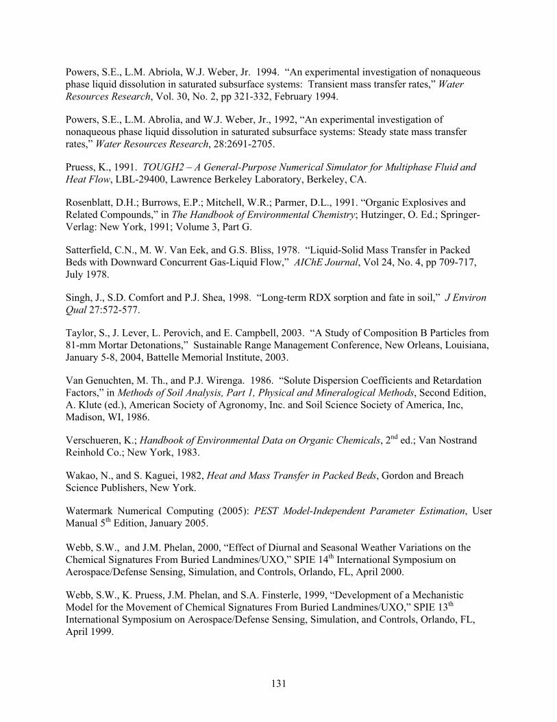
131
Powers, S.E., L.M. Abriola, W.J. Weber, Jr. 1994. “An experimental investigation of nonaqueous phase liquid dissolution in saturated subsurface systems: Transient mass transfer rates,” Water Resources Research, Vol. 30, No. 2, pp 321-332, February 1994.
Powers, S.E., L.M. Abrolia, and W.J. Weber, Jr., 1992, “An experimental investigation of nonaqueous phase liquid dissolution in saturated subsurface systems: Steady state mass transfer rates,” Water Resources Research, 28:2691-2705.
Pruess, K., 1991. TOUGH2 – A General-Purpose Numerical Simulator for Multiphase Fluid and Heat Flow, LBL-29400, Lawrence Berkeley Laboratory, Berkeley, CA.
Rosenblatt, D.H.; Burrows, E.P.; Mitchell, W.R.; Parmer, D.L., 1991. “Organic Explosives and Related Compounds,” in The Handbook of Environmental Chemistry; Hutzinger, O. Ed.; Springer-Verlag: New York, 1991; Volume 3, Part G.
Satterfield, C.N., M. W. Van Eek, and G.S. Bliss, 1978. “Liquid-Solid Mass Transfer in Packed Beds with Downward Concurrent Gas-Liquid Flow,” AIChE Journal, Vol 24, No. 4, pp 709-717, July 1978.
Singh, J., S.D. Comfort and P.J. Shea, 1998. “Long-term RDX sorption and fate in soil,” J Environ Qual 27:572-577.
Taylor, S., J. Lever, L. Perovich, and E. Campbell, 2003. “A Study of Composition B Particles from 81-mm Mortar Detonations,” Sustainable Range Management Conference, New Orleans, Louisiana, January 5-8, 2004, Battelle Memorial Institute, 2003.
Van Genuchten, M. Th., and P.J. Wirenga. 1986. “Solute Dispersion Coefficients and Retardation Factors,” in Methods of Soil Analysis, Part 1, Physical and Mineralogical Methods, Second Edition, A. Klute (ed.), American Society of Agronomy, Inc. and Soil Science Society of America, Inc, Madison, WI, 1986.
Verschueren, K.; Handbook of Environmental Data on Organic Chemicals, 2nd ed.; Van Nostrand Reinhold Co.; New York, 1983.
Wakao, N., and S. Kaguei, 1982, Heat and Mass Transfer in Packed Beds, Gordon and Breach Science Publishers, New York.
Watermark Numerical Computing (2005): PEST Model-Independent Parameter Estimation, User Manual 5th Edition, January 2005. Webb, S.W., and J.M. Phelan, 2000, “Effect of Diurnal and Seasonal Weather Variations on the Chemical Signatures From Buried Landmines/UXO,” SPIE 14th International Symposium on Aerospace/Defense Sensing, Simulation, and Controls, Orlando, FL, April 2000.
Webb, S.W., K. Pruess, J.M. Phelan, and S.A. Finsterle, 1999, “Development of a Mechanistic Model for the Movement of Chemical Signatures From Buried Landmines/UXO,” SPIE 13th International Symposium on Aerospace/Defense Sensing, Simulation, and Controls, Orlando, FL, April 1999.

132
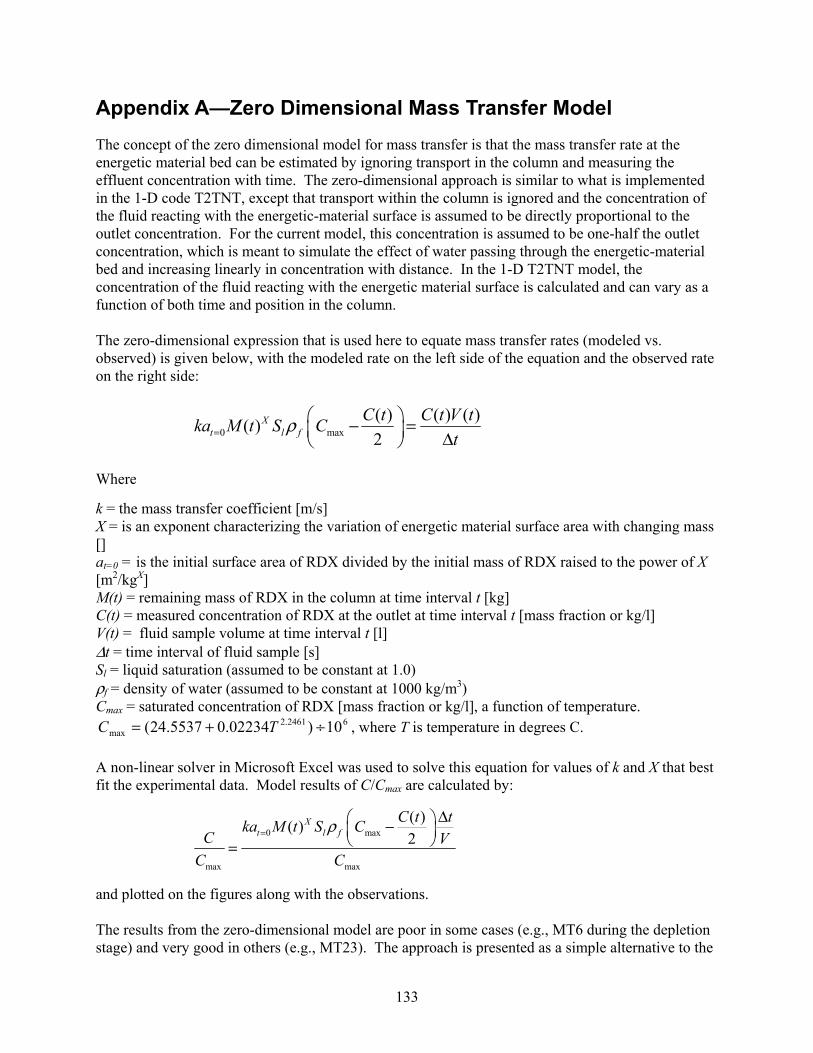
133
Appendix A—Zero Dimensional Mass Transfer Model The concept of the zero dimensional model for mass transfer is that the mass transfer rate at the energetic material bed can be estimated by ignoring transport in the column and measuring the effluent concentration with time. The zero-dimensional approach is similar to what is implemented in the 1-D code T2TNT, except that transport within the column is ignored and the concentration of the fluid reacting with the energetic-material surface is assumed to be directly proportional to the outlet concentration. For the current model, this concentration is assumed to be one-half the outlet concentration, which is meant to simulate the effect of water passing through the energetic-material bed and increasing linearly in concentration with distance. In the 1-D T2TNT model, the concentration of the fluid reacting with the energetic material surface is calculated and can vary as a function of both time and position in the column. The zero-dimensional expression that is used here to equate mass transfer rates (modeled vs. observed) is given below, with the modeled rate on the left side of the equation and the observed rate on the right side:
0 max( ) ( ) ( )( )2
Xt l f
C t C t V tka M t S Ct
ρ=⎛ ⎞− =⎜ ⎟ Δ⎝ ⎠
Where
k = the mass transfer coefficient [m/s] X = is an exponent characterizing the variation of energetic material surface area with changing mass [] at=0 = is the initial surface area of RDX divided by the initial mass of RDX raised to the power of X [m2/kgX] M(t) = remaining mass of RDX in the column at time interval t [kg] C(t) = measured concentration of RDX at the outlet at time interval t [mass fraction or kg/l] V(t) = fluid sample volume at time interval t [l] Δt = time interval of fluid sample [s] Sl = liquid saturation (assumed to be constant at 1.0) ρf = density of water (assumed to be constant at 1000 kg/m3) Cmax = saturated concentration of RDX [mass fraction or kg/l], a function of temperature.
62461.2max 10)02234.05537.24( ÷+= TC , where T is temperature in degrees C.
A non-linear solver in Microsoft Excel was used to solve this equation for values of k and X that best fit the experimental data. Model results of C/Cmax are calculated by:
0 max
max max
( )( )2
Xt l f
C t tka M t S CC V
C C
ρ=Δ⎛ ⎞−⎜ ⎟
⎝ ⎠=
and plotted on the figures along with the observations. The results from the zero-dimensional model are poor in some cases (e.g., MT6 during the depletion stage) and very good in others (e.g., MT23). The approach is presented as a simple alternative to the
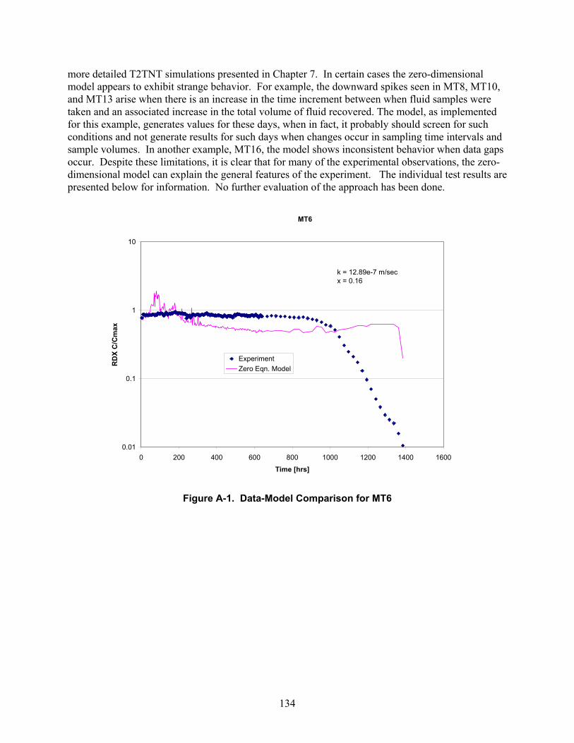
134
more detailed T2TNT simulations presented in Chapter 7. In certain cases the zero-dimensional model appears to exhibit strange behavior. For example, the downward spikes seen in MT8, MT10, and MT13 arise when there is an increase in the time increment between when fluid samples were taken and an associated increase in the total volume of fluid recovered. The model, as implemented for this example, generates values for these days, when in fact, it probably should screen for such conditions and not generate results for such days when changes occur in sampling time intervals and sample volumes. In another example, MT16, the model shows inconsistent behavior when data gaps occur. Despite these limitations, it is clear that for many of the experimental observations, the zero-dimensional model can explain the general features of the experiment. The individual test results are presented below for information. No further evaluation of the approach has been done.
MT6
0.01
0.1
1
10
0 200 400 600 800 1000 1200 1400 1600
Time [hrs]
RD
X C
/Cm
ax
ExperimentZero Eqn. Model
k = 12.89e-7 m/secx = 0.16
Figure A-1. Data-Model Comparison for MT6
135
MT7
0.01
0.1
1
0 50 100 150 200 250
Time [hrs]
C/C
max
ExperimentZero Eqn. Model
k = 4.84e-6 m/secx =1.28
Figure A-2. Data-Model Comparison for MT7
MT8
0.01
0.1
1
10
0 20 40 60 80 100 120 140
Time [hrs]
RD
X C
/Cm
ax
ExperimentZero Eqn. Model
k = 2.39e-5 m/secx = 2.79
Figure A-3. Data-Model Comparison for MT8
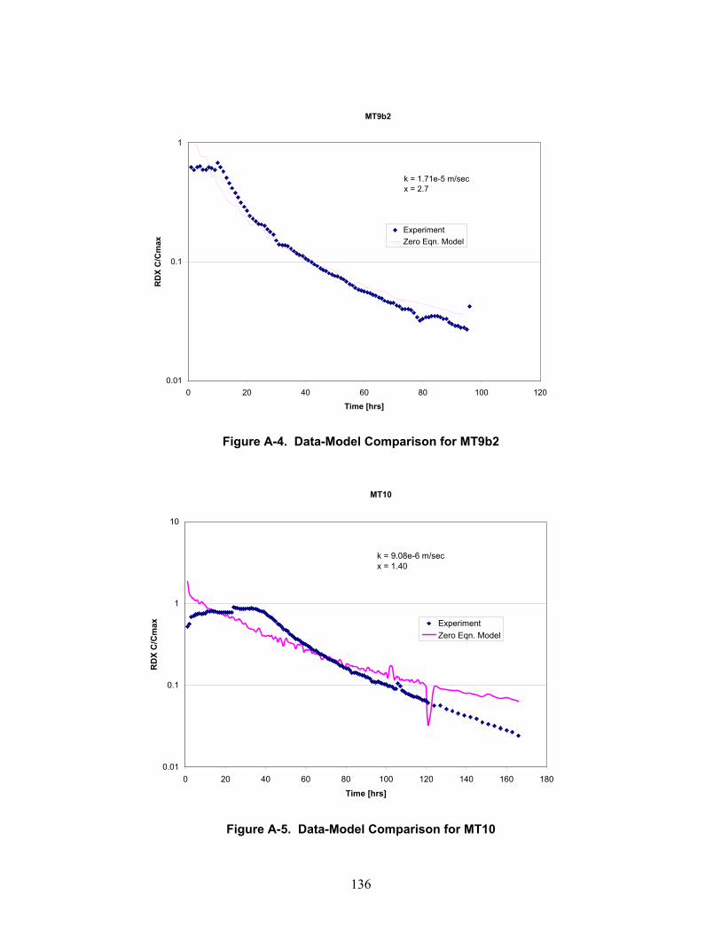
136
MT9b2
0.01
0.1
1
0 20 40 60 80 100 120
Time [hrs]
RD
X C
/Cm
ax
ExperimentZero Eqn. Model
k = 1.71e-5 m/secx = 2.7
Figure A-4. Data-Model Comparison for MT9b2
MT10
0.01
0.1
1
10
0 20 40 60 80 100 120 140 160 180
Time [hrs]
RD
X C
/Cm
ax ExperimentZero Eqn. Model
k = 9.08e-6 m/secx = 1.40
Figure A-5. Data-Model Comparison for MT10
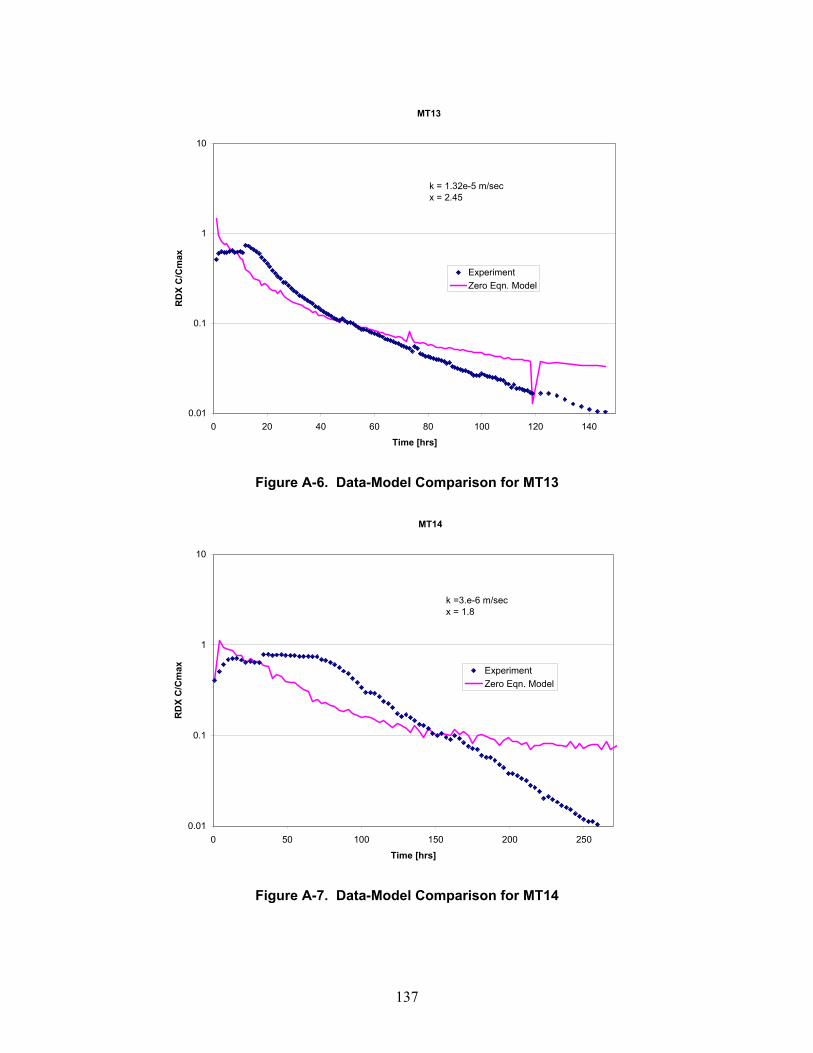
137
MT13
0.01
0.1
1
10
0 20 40 60 80 100 120 140
Time [hrs]
RD
X C
/Cm
ax
ExperimentZero Eqn. Model
k = 1.32e-5 m/secx = 2.45
Figure A-6. Data-Model Comparison for MT13
MT14
0.01
0.1
1
10
0 50 100 150 200 250
Time [hrs]
RD
X C
/Cm
ax ExperimentZero Eqn. Model
k =3.e-6 m/secx = 1.8
Figure A-7. Data-Model Comparison for MT14
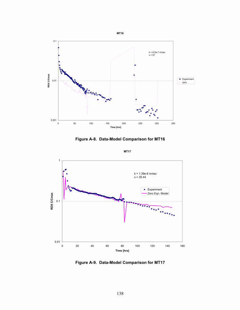
138
MT16
0.001
0.01
0.1
0 50 100 150 200 250 300 350
Time [hrs]
RD
X C
/Cm
ax
Experimentzero
k = 6.0e-7 m/secx = 57
Figure A-8. Data-Model Comparison for MT16
MT17
0.01
0.1
1
0 20 40 60 80 100 120 140 160
Time [hrs]
RD
X C
/Cm
ax
ExperimentZero Eqn. Model
k = 1.39e-6 m/secx = 35.44
Figure A-9. Data-Model Comparison for MT17
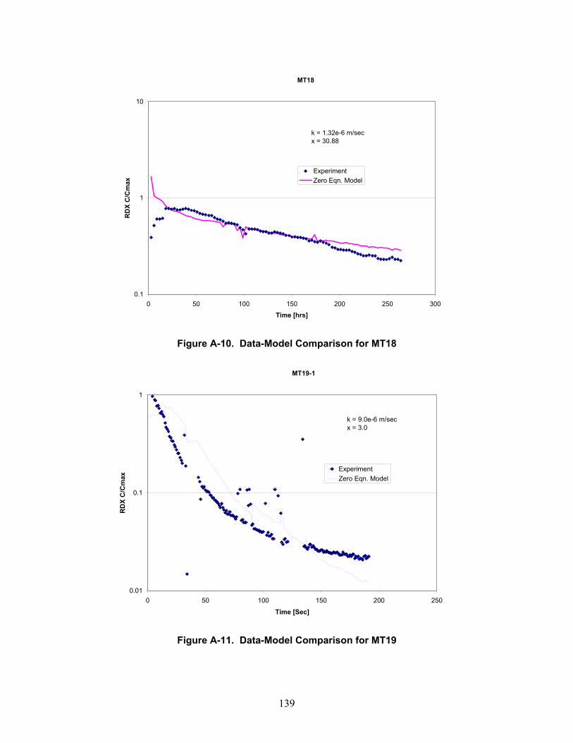
139
MT18
0.1
1
10
0 50 100 150 200 250 300
Time [hrs]
RD
X C
/Cm
ax
ExperimentZero Eqn. Model
k = 1.32e-6 m/secx = 30.88
Figure A-10. Data-Model Comparison for MT18
MT19-1
0.01
0.1
1
0 50 100 150 200 250
Time [Sec]
RD
X C
/Cm
ax
ExperimentZero Eqn. Model
k = 9.0e-6 m/secx = 3.0
Figure A-11. Data-Model Comparison for MT19
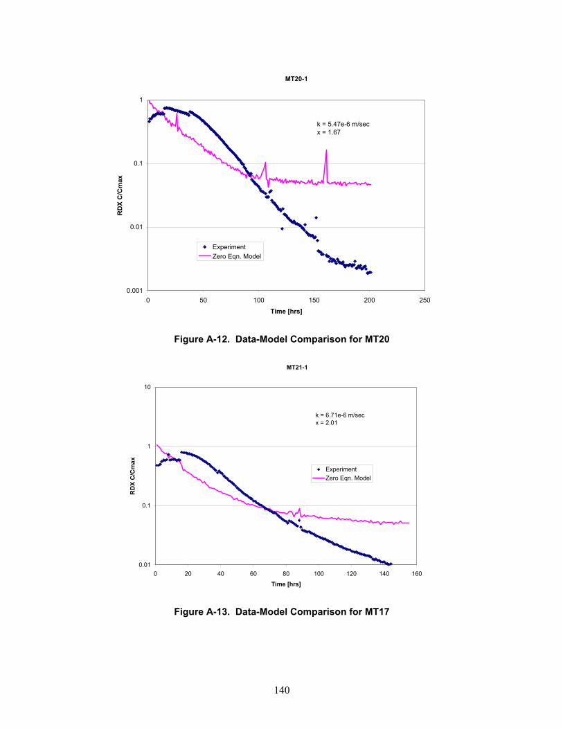
140
MT20-1
0.001
0.01
0.1
1
0 50 100 150 200 250
Time [hrs]
RD
X C
/Cm
ax
ExperimentZero Eqn. Model
k = 5.47e-6 m/secx = 1.67
Figure A-12. Data-Model Comparison for MT20
MT21-1
0.01
0.1
1
10
0 20 40 60 80 100 120 140 160
Time [hrs]
RD
X C
/Cm
ax
ExperimentZero Eqn. Model
k = 6.71e-6 m/secx = 2.01
Figure A-13. Data-Model Comparison for MT17
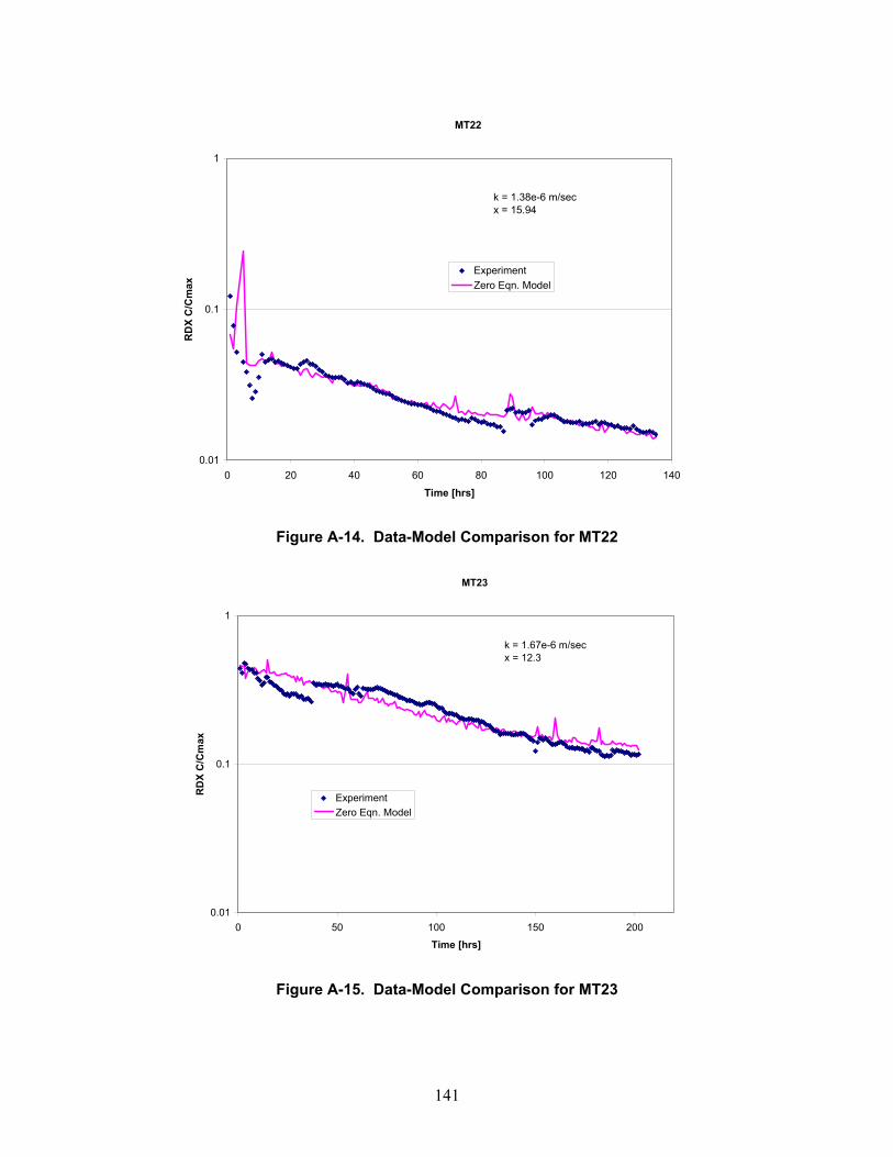
141
MT22
0.01
0.1
1
0 20 40 60 80 100 120 140
Time [hrs]
RD
X C
/Cm
ax
ExperimentZero Eqn. Model
k = 1.38e-6 m/secx = 15.94
Figure A-14. Data-Model Comparison for MT22
MT23
0.01
0.1
1
0 50 100 150 200
Time [hrs]
RD
X C
/Cm
ax
ExperimentZero Eqn. Model
k = 1.67e-6 m/secx = 12.3
Figure A-15. Data-Model Comparison for MT23
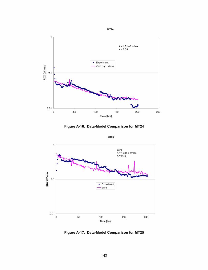
142
MT24
0.01
0.1
1
0 50 100 150 200 250
Time [hrs]
RD
X C
/Cm
ax
ExperimentZero Eqn. Model
k = 1.81e-6 m/secx = 8.05
Figure A-16. Data-Model Comparison for MT24
MT25
0.01
0.1
1
0 50 100 150 200
Time [hrs]
RD
X C
/Cm
ax
ExperimentZero
ZeroK = 1.33e-6 m/secX = 9.75
Figure A-17. Data-Model Comparison for MT25
143
Appendix B—Mass Transfer Parameter Regression Analysis
Description of the Methodology
Data Transformation
In order to perform the sensitivity analysis study, some transformations have been applied to the data. Two of the input parameters, flow direction and bed location, have qualitative values assigned, while we need numerical values. Some arbitrary numbers have thus been assigned to these parameters. For flow direction, downward flow is represented with the number 0, while upward flow is represented with the value 1. For bed location, “center” is represented with the value 1, while “top” is represented with the value 2. The methods used for sensitivity analysis capture linear relationship between the input parameters and the output variables. It is possible to extend these methods to include monotonic relationships by simply working with the rank of the data, instead of the raw values. For each parameter (whether it is an input parameter or output variable), ranked values are obtained by assigning the rank of 1 to the highest value, 2 to the next highest value, and so on. Identical values are assigned with the same rank number. Correlation Matrix
The correlation matrix is calculated by considering all inputs and outputs, and calculating the coefficients of correlation (CC) between every possible paired set. The correlation matrix tells us whether the input parameters are important with respect to the output variables. By looking at the correlation between the input parameters, we can also determine if correlations exist amongst the inputs and whether these correlations could influence the correlation between input and output. The relevant parameters calculated are:
• CC: Correlation Coefficient—Coefficient of correlation between two variables • RCC: Rank Correlation Coefficient—Coefficient of correlations applied to the rank of the
values. Partial (Rank) Correlation Coefficients
As noted in the previous paragraph, the correlation between two input parameters can hide the influence of one input parameter on the output of interest. The partial correlation coefficients (PCC) are used to measure the linear relationship between two variables after removal of effects of other variables. The relevant parameters calculated are:
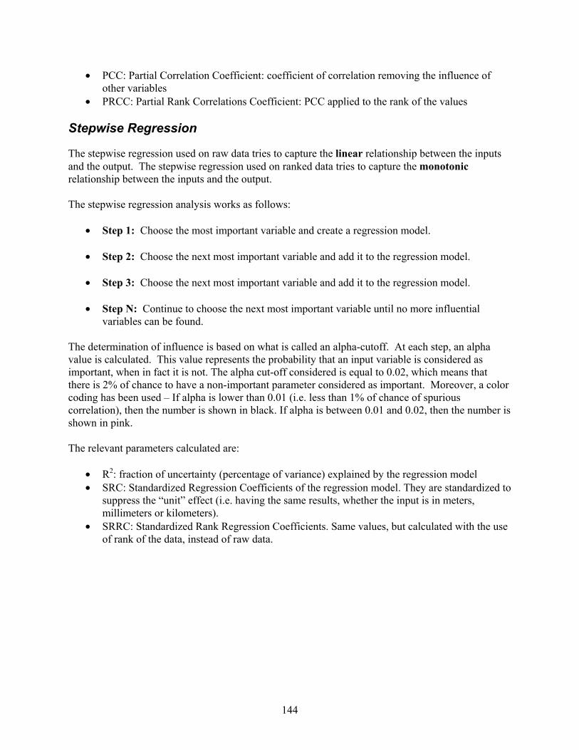
144
• PCC: Partial Correlation Coefficient: coefficient of correlation removing the influence of other variables
• PRCC: Partial Rank Correlations Coefficient: PCC applied to the rank of the values Stepwise Regression
The stepwise regression used on raw data tries to capture the linear relationship between the inputs and the output. The stepwise regression used on ranked data tries to capture the monotonic relationship between the inputs and the output. The stepwise regression analysis works as follows:
• Step 1: Choose the most important variable and create a regression model.
• Step 2: Choose the next most important variable and add it to the regression model.
• Step 3: Choose the next most important variable and add it to the regression model.
• Step N: Continue to choose the next most important variable until no more influential
variables can be found.
The determination of influence is based on what is called an alpha-cutoff. At each step, an alpha value is calculated. This value represents the probability that an input variable is considered as important, when in fact it is not. The alpha cut-off considered is equal to 0.02, which means that there is 2% of chance to have a non-important parameter considered as important. Moreover, a color coding has been used – If alpha is lower than 0.01 (i.e. less than 1% of chance of spurious correlation), then the number is shown in black. If alpha is between 0.01 and 0.02, then the number is shown in pink. The relevant parameters calculated are:
• R2: fraction of uncertainty (percentage of variance) explained by the regression model • SRC: Standardized Regression Coefficients of the regression model. They are standardized to
suppress the “unit” effect (i.e. having the same results, whether the input is in meters, millimeters or kilometers).
• SRRC: Standardized Rank Regression Coefficients. Same values, but calculated with the use of rank of the data, instead of raw data.
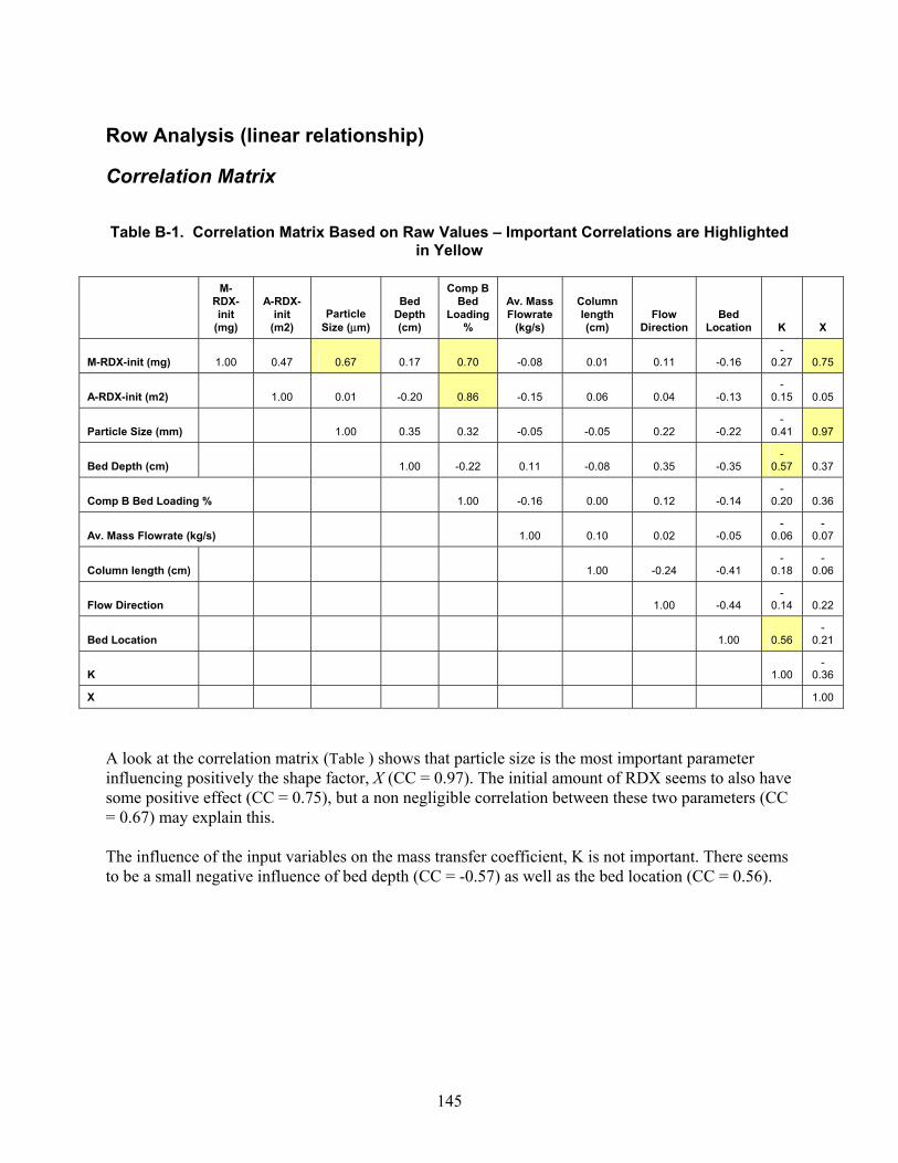
145
Row Analysis (linear relationship)
Correlation Matrix
Table B-1. Correlation Matrix Based on Raw Values – Important Correlations are Highlighted in Yellow
M-RDX-init
(mg)
A-RDX-init
(m2) Particle
Size (μm)
Bed Depth (cm)
Comp B Bed
Loading %
Av. Mass Flowrate
(kg/s)
Column length (cm)
Flow Direction
Bed Location K X
M-RDX-init (mg) 1.00 0.47 0.67 0.17 0.70 -0.08 0.01 0.11 -0.16 -
0.27 0.75
A-RDX-init (m2) 1.00 0.01 -0.20 0.86 -0.15 0.06 0.04 -0.13 -
0.15 0.05
Particle Size (mm) 1.00 0.35 0.32 -0.05 -0.05 0.22 -0.22 -
0.41 0.97
Bed Depth (cm) 1.00 -0.22 0.11 -0.08 0.35 -0.35 -
0.57 0.37
Comp B Bed Loading % 1.00 -0.16 0.00 0.12 -0.14 -
0.20 0.36
Av. Mass Flowrate (kg/s) 1.00 0.10 0.02 -0.05 -
0.06 -
0.07
Column length (cm) 1.00 -0.24 -0.41 -
0.18 -
0.06
Flow Direction 1.00 -0.44 -
0.14 0.22
Bed Location 1.00 0.56 -
0.21
K 1.00 -
0.36
X 1.00
A look at the correlation matrix (Table ) shows that particle size is the most important parameter influencing positively the shape factor, X (CC = 0.97). The initial amount of RDX seems to also have some positive effect (CC = 0.75), but a non negligible correlation between these two parameters (CC = 0.67) may explain this. The influence of the input variables on the mass transfer coefficient, K is not important. There seems to be a small negative influence of bed depth (CC = -0.57) as well as the bed location (CC = 0.56).
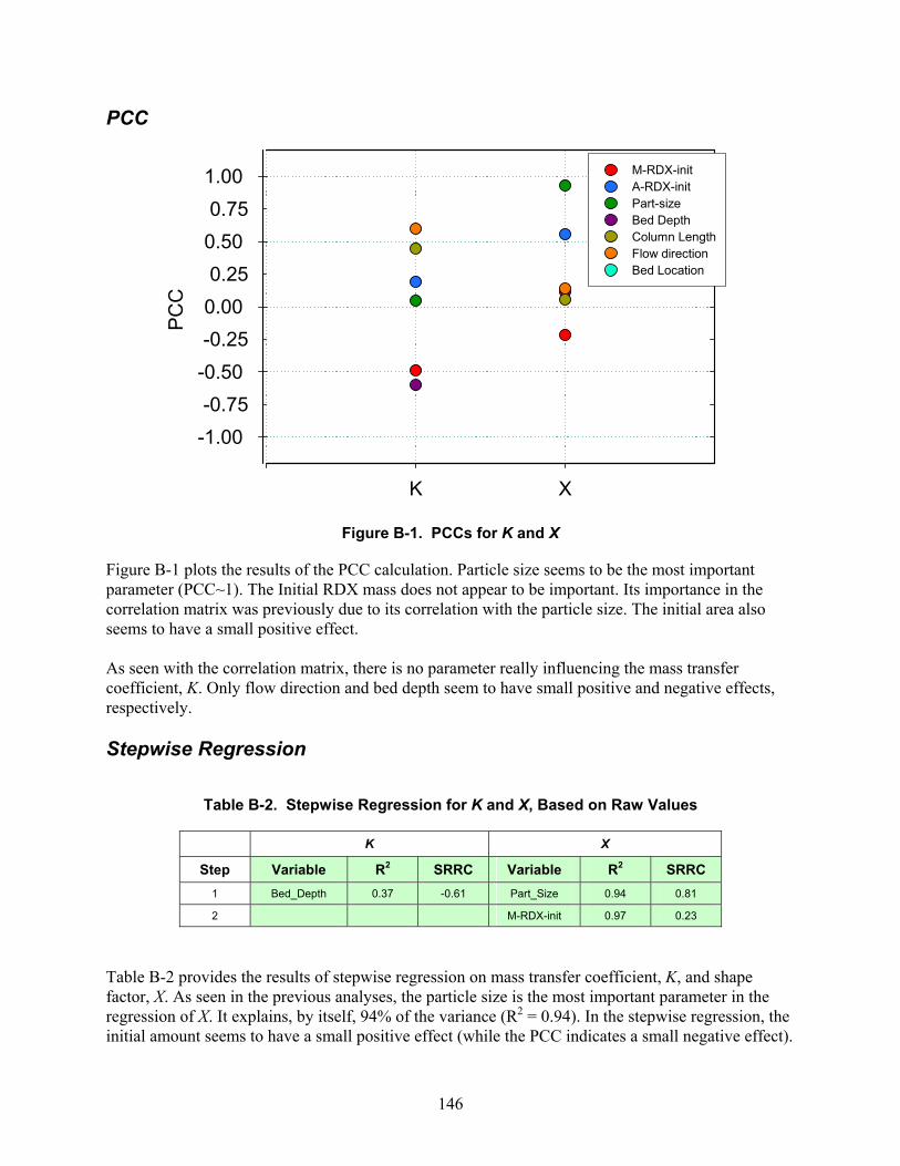
146
PCC
K X
PC
C
-0.75
-0.25
0.25
0.75
-1.00
-0.50
0.00
0.50
1.00 M-RDX-initA-RDX-initPart-sizeBed DepthColumn LengthFlow direction Bed Location
Figure B-1. PCCs for K and X
Figure B-1 plots the results of the PCC calculation. Particle size seems to be the most important parameter (PCC~1). The Initial RDX mass does not appear to be important. Its importance in the correlation matrix was previously due to its correlation with the particle size. The initial area also seems to have a small positive effect. As seen with the correlation matrix, there is no parameter really influencing the mass transfer coefficient, K. Only flow direction and bed depth seem to have small positive and negative effects, respectively. Stepwise Regression
Table B-2. Stepwise Regression for K and X, Based on Raw Values
K X
Step Variable R2 SRRC Variable R2 SRRC 1 Bed_Depth 0.37 -0.61 Part_Size 0.94 0.81
2 M-RDX-init 0.97 0.23
Table B-2 provides the results of stepwise regression on mass transfer coefficient, K, and shape factor, X. As seen in the previous analyses, the particle size is the most important parameter in the regression of X. It explains, by itself, 94% of the variance (R2 = 0.94). In the stepwise regression, the initial amount seems to have a small positive effect (while the PCC indicates a small negative effect).
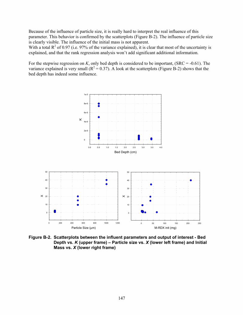
147
Because of the influence of particle size, it is really hard to interpret the real influence of this parameter. This behavior is confirmed by the scatterplots (Figure B-2). The influence of particle size is clearly visible. The influence of the initial mass is not apparent. With a total R2 of 0.97 (i.e. 97% of the variance explained), it is clear that most of the uncertainty is explained, and that the rank regression analysis won’t add significant additional information. For the stepwise regression on K, only bed depth is considered to be important, (SRC = -0.61). The variance explained is very small (R2 = 0.37). A look at the scatterplots (Figure B-2) shows that the bed depth has indeed some influence.
Bed Depth (cm)0.0 0.5 1.0 1.5 2.0 2.5 3.0 3.5 4.0
K
0
2e-6
4e-6
6e-6
8e-6
1e-5
Particle Size (μm)
0 200 400 600 800 1000 1200
X
0
10
20
30
40
50
M-RDX init (mg)0 50 100 150 200 250
X
0
10
20
30
40
50
Figure B-2. Scatterplots between the influent parameters and output of interest - Bed Depth vs. K (upper frame) – Particle size vs. X (lower left frame) and Initial Mass vs. X (lower right frame)
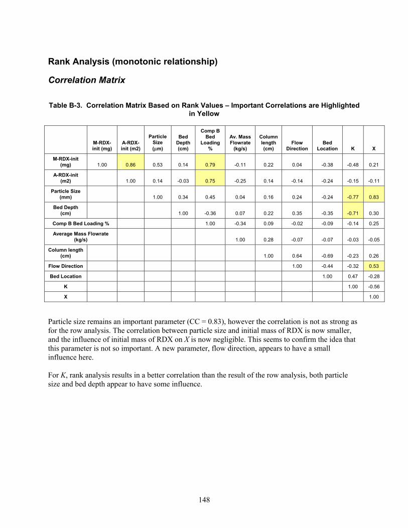
148
Rank Analysis (monotonic relationship)
Correlation Matrix
Table B-3. Correlation Matrix Based on Rank Values – Important Correlations are Highlighted in Yellow
M-RDX-init (mg)
A-RDX-init (m2)
Particle Size (μm)
Bed Depth (cm)
Comp B Bed
Loading %
Av. Mass Flowrate
(kg/s)
Column length (cm)
Flow Direction
Bed Location K X
M-RDX-init (mg) 1.00 0.86 0.53 0.14 0.79 -0.11 0.22 0.04 -0.38 -0.48 0.21
A-RDX-init (m2) 1.00 0.14 -0.03 0.75 -0.25 0.14 -0.14 -0.24 -0.15 -0.11
Particle Size (mm) 1.00 0.34 0.45 0.04 0.16 0.24 -0.24 -0.77 0.83
Bed Depth (cm) 1.00 -0.36 0.07 0.22 0.35 -0.35 -0.71 0.30
Comp B Bed Loading % 1.00 -0.34 0.09 -0.02 -0.09 -0.14 0.25
Average Mass Flowrate (kg/s) 1.00 0.28 -0.07 -0.07 -0.03 -0.05
Column length (cm) 1.00 0.64 -0.69 -0.23 0.26
Flow Direction 1.00 -0.44 -0.32 0.53
Bed Location 1.00 0.47 -0.28
K 1.00 -0.56
X 1.00
Particle size remains an important parameter (CC = 0.83), however the correlation is not as strong as for the row analysis. The correlation between particle size and initial mass of RDX is now smaller, and the influence of initial mass of RDX on X is now negligible. This seems to confirm the idea that this parameter is not so important. A new parameter, flow direction, appears to have a small influence here. For K, rank analysis results in a better correlation than the result of the row analysis, both particle size and bed depth appear to have some influence.
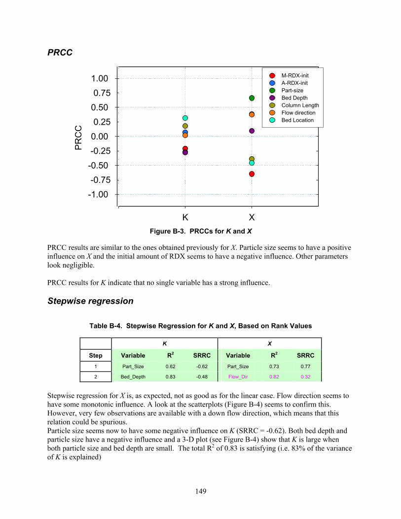
149
PRCC
K X
PR
CC
-0.75
-0.25
0.25
0.75
-1.00
-0.50
0.00
0.50
1.00 M-RDX-initA-RDX-initPart-sizeBed DepthColumn LengthFlow direction Bed Location
Figure B-3. PRCCs for K and X
PRCC results are similar to the ones obtained previously for X. Particle size seems to have a positive influence on X and the initial amount of RDX seems to have a negative influence. Other parameters look negligible. PRCC results for K indicate that no single variable has a strong influence. Stepwise regression
Table B-4. Stepwise Regression for K and X, Based on Rank Values
K X
Step Variable R2 SRRC Variable R2 SRRC 1 Part_Size 0.62 -0.62 Part_Size 0.73 0.77
2 Bed_Depth 0.83 -0.48 Flow_Dir 0.82 0.32
Stepwise regression for X is, as expected, not as good as for the linear case. Flow direction seems to have some monotonic influence. A look at the scatterplots (Figure B-4) seems to confirm this. However, very few observations are available with a down flow direction, which means that this relation could be spurious. Particle size seems now to have some negative influence on K (SRRC = -0.62). Both bed depth and particle size have a negative influence and a 3-D plot (see Figure B-4) show that K is large when both particle size and bed depth are small. The total R2 of 0.83 is satisfying (i.e. 83% of the variance of K is explained)
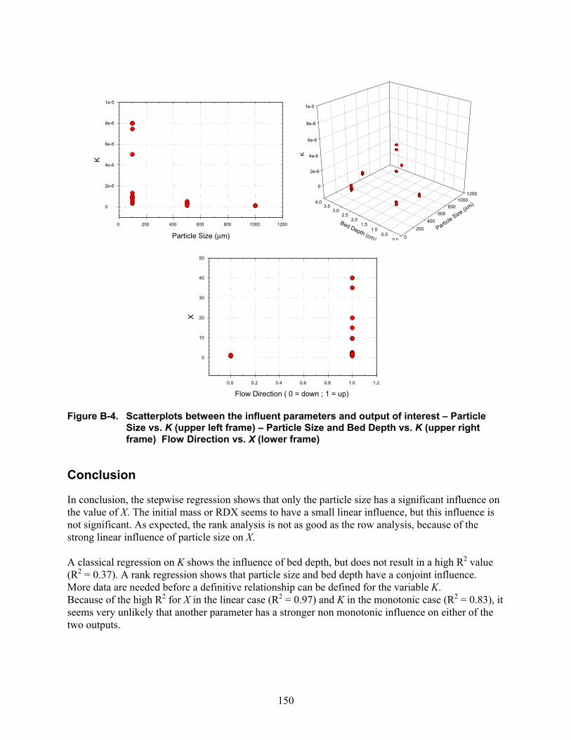
150
Particle Size (μm)
0 200 400 600 800 1000 1200
K
0
2e-6
4e-6
6e-6
8e-6
1e-5
0
2e-6
4e-6
6e-6
8e-6
1e-5
0
200
400600
8001000
1200
0 00.5
1.01.5
2.02.5
3.03.5
4.0
K
Particle Size
(μm)
Bed Depth (cm)
Flow Direction ( 0 = down ; 1 = up) 0.0 0.2 0.4 0.6 0.8 1.0 1.2
X
0
10
20
30
40
50
Figure B-4. Scatterplots between the influent parameters and output of interest – Particle Size vs. K (upper left frame) – Particle Size and Bed Depth vs. K (upper right frame) Flow Direction vs. X (lower frame)
Conclusion
In conclusion, the stepwise regression shows that only the particle size has a significant influence on the value of X. The initial mass or RDX seems to have a small linear influence, but this influence is not significant. As expected, the rank analysis is not as good as the row analysis, because of the strong linear influence of particle size on X. A classical regression on K shows the influence of bed depth, but does not result in a high R2 value (R2 = 0.37). A rank regression shows that particle size and bed depth have a conjoint influence. More data are needed before a definitive relationship can be defined for the variable K. Because of the high R2 for X in the linear case (R2 = 0.97) and K in the monotonic case (R2 = 0.83), it seems very unlikely that another parameter has a stronger non monotonic influence on either of the two outputs.
151
Distribution Internal 1 MS0735 S.W. Webb, 6115 1 MS0782 J.M. Phelan, 6418 1 MS0776 J.S. Stein, 6852 1 MS0776 T. Hadgu, 6852 1 MS0776 C.M. Sallaberry, 6852 2 MS9960 Central Technical Files, 8945-1 2 MS0899 Technical Library, 04536 External 1 Deanne Rider
SERDP/ESTCP Support Office HydroGeoLogic, Inc. 1155 Herndon Parkway, Suite 900 Herndon, VA 20170
Electronic – SERDP/ESTCP Jeffrey Marqusee ([email protected])
Andrea Leeson ([email protected]) Robert Holst ([email protected]) Kelly Woodworth ([email protected]) Amir Abyaneh ([email protected]) Deanne Rider ([email protected])