measurement and comparison of solar...
TRANSCRIPT
MEASUREMENT AND COMPARISON OF SOLAR RADIATION ESTIMATION MODELS FOR IZMIR/TURKEY: IZMIR INSTITUTE OF
TECHNOLOGY CASE
A Thesis Submitted to the Graduate School of Engineering and Sciences of
Izmir Institute of Technology in Partial Fulfilment of the Requirements for the Degree of
MASTER OF SCIENCE
in Mechanical Engineering
by Didem VECAN
September 2011 İZMİR
We approve the thesis of Didem VECAN
Prof. Dr. Barış ÖZERDEM Supervisor Prof. Dr. Zafer İLKEN Committee Member Assoc. Prof. Dr. Serhan KÜÇÜKA Committee Member 28 September 2011
Prof. Dr. Metin TANOĞLU Prof. Dr. R. Tuğrul SENGER Head of the Department of Dean of the School of Mechanical Engineering Engineering and Sciences

ACKNOWLEDGEMENTS
First of all, the author wishes to express her gratitude to her supervisor Prof. Dr.
Barış Özerdem for his valuable guidance, continual support and supervision throughout
this study.
The author would like to thank Assist. Prof. Dr. Koray Ülgen for his support and
help.
Finally, the author would like to give her special thanks to her family for their
support and encouragements during her education.
iv
ABSTRACT
MEASUREMENT AND COMPARISON OF SOLAR RADIATION ESTIMATION MODELS FOR IZMIR/TURKEY: IZMIR INSTITUTE OF
TECHNOLOGY CASE
Solar energy technologies offer a clean, renewable and domestic energy source,
and are essential components of a sustainable energy in the future. Proper and adequate
information on solar radiation and its components at a given location is very essential in
the design of solar energy systems. Due to Turkey’s location, solar energy potential is
abundantly available. Consequently, it is worth to examine and conduct research on the
solar energy source.
In this study, the global solar radiation data in Izmir were analyzed based on 3
years of global solar radiation data measured on a horizontal surface on the campus area
of Izmir Institute of Technology. Actual data readings were made on a ten minute basis
from January, 2005 to December, 2007. Monthly-average daily global radiation has
been analyzed. A linear, a second-order and third order equations are designed for the
calculation of the monthly-average daily global radiation in Izmir. The main objective is
to estimate global solar radiation via models mentioned in the literature both for Turkey
in general and for Izmir specifically; and to compare the results with the three new
developed models. In addition to global solar radiation, diffuse solar radiation data were
analyzed and proposed models for estimating the monthly average daily diffuse solar
radiation, as well. Four new models were developed for diffuse solar radiation
calculations and nine models from the literature have been used.
In order to confirm the results, four statistical methods have been used namely;
mean bias error (MBE), root mean square (RMSE), t-statistic and relative percentage
error. According to the statistical evaluation, it may be concluded that the new
polynomial equation predict the monthly-average daily global solar radiance better than
other available models.
v
ÖZET
İZMİR/TÜRKİYE İÇİN GÜNEŞ IŞINIM TAHMİN MODELLERİNİN ÖLÇÜM VE KARŞILAŞTIRMALARI: İZMİR YÜKSEK TEKNOLOJİ
ENSTİTÜSÜ DURUM ÇALIŞMALARI
Güneş enerjisi yenilenebilir, temiz ve sürdürülebilir yerli enerji kaynağıdır. Bu
nedenle gelecekteki en temel enerji elemanı olarak görülmektedir. Güneş enerjisine ait
tasarım ve çalışmalarda, belirli bir bölge için güneş ışınımı ve bileşenlerine ait bilgiler
önem taşımaktadır. Türkiye konumu nedeniyle yüksek bir güneş enerjisi potansiyeline
sahiptir ve bu sebeple güneş enerjisi verilerini incelemek ve çalışmalar yapmak önem
taşımaktadır.
Bu çalışmada İzmir Yüksek Teknoloji Enstitüsü’nde yatay bir alanda küresel
güneş ışınım değerleri üç sene boyunca on ’ar dakikalık aralıklarla 2005 Ocak başından
2007 Aralık sonuna kadar ölçülmüştür. Bu veriler kullanılarak aylık ortalama günlük
global ışınım belirlenmiştir. Literatürde Türkiye geneli ve sadece İzmir için daha önce
çalışılmış 10 model kullanılarak aylık ortalama günlük global güneş ışınımı
hesaplanmıştır. Ayrıca İzmir için lineer, ikinci ve üçüncü dereceden eşitlikler
geliştirilmiştir. Bunun yanında, yaygın güneş ışınımı ile ilgili de benzer çalışmalar
yapılmıştır. Literatürde yer alan Türkiye ve genel modellemelerden ve İzmir için
ölçülmüş verilerden yola çıkılarak denklemler geliştirilmiş ve karşılaştırılmıştır.
Eşitliklerin ve modellerin performans değerlendirmesi için ortalama hata (MBE),
tahmini standart hataları (RMSE) ve t-istatistik yöntemleri kullanılmıştır. Yapılan
karşılaştırmalar sonucunda 2. derece geliştirilen eşitliğin diğer modellere oranla daha
başarılı sonuç verdiği görülmüştür.
vi
TABLE OF CONTENTS
LIST OF FIGURES………………………………………………………………...
LIST OF TABLES………………………………………………………………….
LIST OF SYMBOLS……………………………………………………………….
LIST OF ABBREVIATIONS……………………………………………………...
CHAPTER 1. INTRODUCTION…………………………………………………..
CHAPTER 2. LITERATURE SURVEY…………………………………………..
2.1. Global Solar Radiation……………………………………………
2.2. Diffuse Solar Radiation…………………………………………...
CHAPTER 3. EXPERIMENTAL SOLAR RADIATION DATA AND
STATISTICAL METHODS………………………………………...
3.1. Experimental data…………………………………………………
3.2. Statistical methods………………………………………………...
3.2.1. Mean Bias Error…………………………………………………
3.2.2. Root Mean Square Error………………………………………...
3.2.3. t-Statistic Method……………………………………………….
3.2.4. Relative Percentage Error……………………………………….
CHAPTER 4. ANALYSIS OF GLOBAL RADIATION MODELS……………….
4.1. Kılıc and Ozturk’s Model………………………………………….
4.2. Akinoglu and Ecevit’s Model……………………………………...
4.3. Tasdemiroglu and Sever’s Model………………………………….
4.4. Oz’s Model………………………………………………………...
4.5. Aksoy’s Model…………………………………………………….
4.6. Ulgen and Ozbalta’s Model………………………………………..
4.7. Togrul and Togrul’s Model………………………………………..
viii
ix
x
xi
1
8
8
12
15
15
18
18
18
19
19
20
20
20
21
21
21
21
21
vii
4.8. Ulgen and Hepbasli’s Model……………………………………....
4.9. Ulgen and Hepbasli’s Model……………………………………....
4.10. New Developed Equation 1……………………………………....
4.11. New Developed Equation 2……………………………………....
4.12. New Developed Equation 3……………………………………....
CHAPTER 5. ANALYSIS OF DIFFUSE RADIATION MODELS……………….
5.1. H as a function of H and the clearness index (Group 1)………….
5.1.1. Tasdemiroglu and Sever’s Model……………………………...
5.1.2. Tiris et al. Model………………………………………………
5.1.3. New Developed Equation A…………………………………...
5.2. H as a function of H and sunshine fraction (Group 2)……………
5.2.1. Barbaro et al.’s Model…………………………………………
5.2.2. Ulgen and Hepbasli’s Model…………………………………..
5.2.3. New Developed Equation B…………………………………...
5.3. H as a function of Hₒ and the clearness index (Group 3)…………
5.3.1. Ulgen and Hepbasli’s Model…………………………………..
5.3.2. Aras et al. Models ……………………………………………..
5.3.3. New Developed Equation C…………………………………...
5.4. H as a function of Hₒ and sunshine fraction (Group 4)…………...
5.4.1. Ulgen and Hepbasli’s Model…………………………………..
5.4.2. Aras et al. Models……………………………………………...
5.4.3. New Developed Equation D…………………………………...
CHAPTER 6. RESULTS…………………………………………………………...
6.1. Results for Global Solar Radiation………………………………...
6.2. Results for Diffuse Solar Radiation………………………………..
CHAPTER 7. CONCLUSION……………………………………………………...
REFERENCES……………………………………………………………………...
APPENDIX A. The monthly-average hourly global solar radiation tables………...
22
22
22
22
23
24
24
24
24
25
25
25
25
25
26
26
26
26
26
26
27
27
28
28
39
44
45
49
viii
LIST OF FIGURES
Figure
Figure 1. Direct, diffuse and reflected solar radiation…………………………….
Figure 2. Approximate construction of CM11…………………………………….
Figure 3. Shadow ring for CM11 pyranometer……………………………………
Figure 4. Data logger…………………………………………………………….
Figure 5. The graph of the monthly-average daily extraterrestrial radiation……...
Figure 6. The graph of the monthly-average hourly global radiation for 2005…..
Figure 7. The graph of the monthly-average hourly global radiation for 2006…...
Figure 8. The graph of the monthly-average hourly global radiation for 2007…...
Figure 9. The graph of the monthly-average hourly global radiation for 3 years
period…………………………………………………………………….
Figure 10. The graph of solar radiation models…………………………………...
Figure 11. The graph of Hₒ………………………………………………………..
Figure 12. The graph of new developed equations for diffuse solar radiation……
Page
4
16
17
17
29
31
32
33
33
37
40
43
ix
LIST OF TABLES
Table
Table 1. Turkey’s monthly-average solar radiation data………………………….
Table 2. CM11 specifications……………………………………………………..
Table 3. Monthly-average of the maximum possible daily hours of bright
sunshine for 2005-2007………………………………………………..
Table 4. Average of bright sunshine hours for 2005-2007………………………..
Table 5. Hₒ values for Izmir………………………………………………………
Table 6. The monthly-average hourly global radiation for 2005………………….
Table 7. The monthly-average hourly global radiation for 2006………………….
Table 8. The monthly-average hourly global radiation for 2007………………….
Table 9. Hourly average global solar radiations for the average of 3 years………
Table 10. Hourly average global solar radiation values for solar radiation models
Table 11. Results of a, b in Eqs. (4.2) and (4.3)…………………………………..
Table 12. Comparison of statistical methods for global solar radiation models…..
Table 13. Measured diffuse solar radiation data…………………………………..
Table 14. The monthly-average daily diffuse solar radiation for models…………
Table 15. Comparison of statistical methods for diffuse solar radiation models…
Page
6
16
28
29
30
30
31
32
35
36
37
38
39
41
42

x
LIST OF SYMBOLS
G
H
H
Hₒ
k
n
S
Sₒ
Z
Φ
δ
푤
k
k
k
Solar constant (1367 W/m²)
Monthly-average daily total radiation (W/m²)
Monthly-average daily extraterrestrial radiation (W/m²)
Monthly-average daily diffuse radiation (W/m²)
Data number
Day of year starting from the 1st of January
The monthly-average daily hours of bright sunshine (h)
The monthly-average of the maximum possible daily hours of bright sunshine (h)
Altitude (m)
The latitude of the area (°)
The solar declination (°)
Sunset hour angle (°)
Clearness index (H/ Hₒ)
Diffuse coefficient (H /Hₒ)
Cloudiness index (H /H)

xi
LIST OF ABBREVIATIONS
DMI
EIEI
IYTE
MBE
RMSE
t-stat
e
MPE
MAPE
SSRE
RSE
CAR
CBSR
IZTECH
Turkish State Meteorological Service
Electrical Works Research Directorate
Izmir Institute Of Technology
Mean Bias Error
Root Mean Square Error
t-statistic method
Relative Percentage Error
Mean Percentage Error
Mean Absolute Percentage Error
Sum of The Squares of Relative Errors
The Relative Standard Error
Central Anatolia Region
Central Black Sea Region
Izmir Institute of Technology
1
CHAPTER 1
INTRODUCTION
Due to the developments in the technology, the energy need of people is
increased. The sources of the energy are varied according to the technological progress.
In the beginning, wood has been used to provide energy, and then coal is replaced
instead of wood. Finding oil and natural gases, energy growth has been assured.
Energy demand is increasing by about 2% a year, and absorbs most of the
requirements for energy development. New technology makes better use of already
available energy through improved efficiency, such as more efficient fluorescent
lamps, engines, and insulation. Using heat exchangers, it is possible to recover some of
the energy in waste warm water and air, for example to preheat incoming fresh water.
Hydrocarbon fuel production from pyrolysis could also be in this category, allowing
recovery of some of the energy in hydrocarbon waste. Already existing power
plants often can and usually are made more efficient with minor modifications due to
new technology. New power plants may become more efficient with technology
like cogeneration. New designs for buildings may incorporate techniques like passive
solar. Light-emitting diodes are gradually replacing the remaining uses of light bulbs.
Renewable energy is considered to be the most important source to the world for
the future. The decrease in the fossil fuels, made an orientation to the renewable energy
sources such as sunlight, wind, rain, tides, and geothermal heat. Renewable energy is an
alternative to fossil fuels and nuclear power, and was commonly called alternative
energy in the 1970s and 1980s. In 2008, about 19% of global final energy consumption
came from renewables, with 13% coming from traditional biomass, which is mainly
used for heating, and 3.2% from hydroelectricity. New renewables (small hydro,
modern biomass, wind, solar, geothermal, and biofuels) accounted for another 2.7% and
are growing very rapidly. The share of renewables in electricity generation is around
18%, with 15% of global electricity coming from hydroelectricity and 3% from new
renewables.
While many renewable energy projects are large-scale, renewable technologies
are also suited to rural and remote areas, where energy is often crucial in human
2
development. Globally, an estimated 3 million households get power from small solar
PV systems. Micro-hydro systems configured into village-scale or county-scale mini-
grids serve many areas. More than 30 million rural households get lighting and cooking
from biogas made in household-scale digesters. Biomass cook stoves are used by 160
million households.
Among the renewable energy resources solar energy is the most actual and
usable in the world. It is the energy obtained from the heat and rays of the sun.
The Sun is the star at the center of the Solar System. It is almost perfectly spherical and
consists of hot plasma interwoven with magnetic fields. It has a diameter of about
1,392,000 km, about 109 times that of Earth, and its mass (about 2×10 kilograms,
330,000 times that of Earth) accounts for about 99.86% of the total mass of the Solar
System. Chemically, about three quarters of the Sun's mass consists of hydrogen, while
the rest is mostly helium. Less than 2% consists of heavier elements,
including oxygen, carbon, neon, iron, and others. The mean distance of the Sun from the
Earth is approximately 149.6 million kilometers, though the distance varies as the Earth
moves from perihelion in January to aphelion in July. At this average
distance, light travels from the Sun to Earth in about 8 minutes and 19 seconds.
The energy of this sunlight supports almost all life on Earth by photosynthesis, and
drives Earth's climate and weather.
Solar energy can be used to generate electricity using photovoltaic solar cells
and concentrated solar power. It can be used to heat buildings directly by passive solar
building designs, or cooking and heating food with the help of solar ovens.
Solar technologies are broadly characterized as either passive solar or active
solar depending on the way they capture, convert and distribute solar energy. Active
solar techniques include the use of photovoltaic panels and solar thermal collectors to
harness the energy. Passive solar techniques include orienting a building to the Sun,
selecting materials with favorable thermal mass or light dispersing properties, and
designing spaces that naturally circulate air.
The flexibility of solar energy is manifest in a wide variety of technologies from
cars and calculators to huge photovoltaic plants. Recent price hikes and erratic
availability of conventional fuels are factors that are renewing interest in solar heating
technologies. Thus solar power is important to the very existence of the world as a
whole.
3
To make use of solar energy in a better way, the feature of the sunlight and the
amount of the solar power on a specific time and place are essential. Since the Sun is
almost 150 million kilometers from the Earth, the energy density per unit time of the
sunlight reaching the upper atmosphere of the Earth is only 1,367 W/m², which is
known as solar constant. The solar constant is the amount of power that the Sun
deposits per unit area that is directly exposed to sunlight.
At the core, solar energy is actually nuclear energy. In the inner 25% of the Sun,
hydrogen is fusing into helium at a rate of about 7 x 10 kg of hydrogen every second.
Heat from the core is first primarily radiated, and then primarily convected, to the Sun’s
surface, where it maintains at a temperature of 5800 K.
The primary method of energy transport is electromagnetic radiation from the
surface of the Sun; this form of heat transport depends greatly upon the surface
temperature of an object for the amount and type of energy. Stefan-Boltzmann’s Law
tells us that the amount of energy that is radiated per unit area of surface depends upon
the temperature of the object to the fourth power, i.e. energy/area is proportional toT .
This means that the amount of energy that is emitted by the Sun, and therefore, the
amount of solar energy that we receive here on Earth, is critically dependent upon this
surface temperature. A change of 1% in the temperature of the Sun (58 K) can result in
a change of 4% in the amount of energy per unit area that the world receives.
The type of radiation coming from the Sun also depends on temperature. The
Sun is emitting electromagnetic radiation in wide variety of wavelengths. However,
most of the radiation is being sent out in the visible spectrum due to its surface
temperature. As an object gets hotter, the peak radiation will come from shorter
wavelengths, and vice-versa.
The Sun radiates 1.6 x 10 watts of power per square meter from its surface at
all wavelengths. However, by the time that it has reached the Earth’s surface, this value
is vastly reduced. Between the Sun’s and the Earth’s surfaces, the energy density of the
radiation is lessened by spreading and absorption.
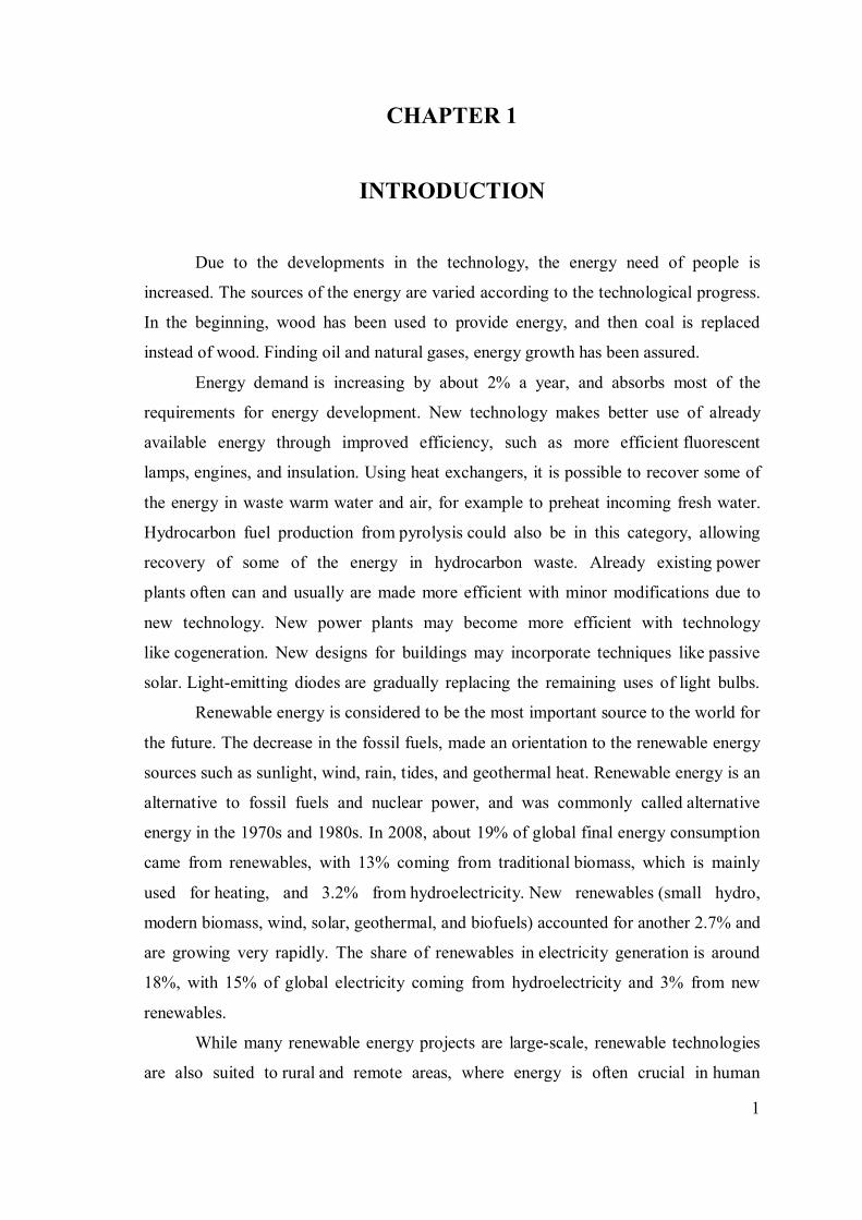
Many people think solar radiation comes in a direct beam from the sun.
However, as radiation from the sun hits our atmosphere some is scattered in all
directions. Some of this radiation is scattered towards the earth and is called diffuse
solar radiation. The amount of solar radiation arriving at a particular point is called
global solar radiation. In other words, in the earth’s atmosphere, solar radiation is
4
received directly (direct radiation) and by diffusion in air, dust, water, etc., contained in
the atmosphere (diffuse radiation). As shown is Figure 1, global radiation is the sum of
the reflected radiation, direct irradiation and the diffuse solar radiation on any plane.
Values of global and diffuse radiations for individual hours are essential for research
and engineering applications.
Figure 1. Direct, diffuse and reflected solar radiation
(Source: inforse; June, 2010)
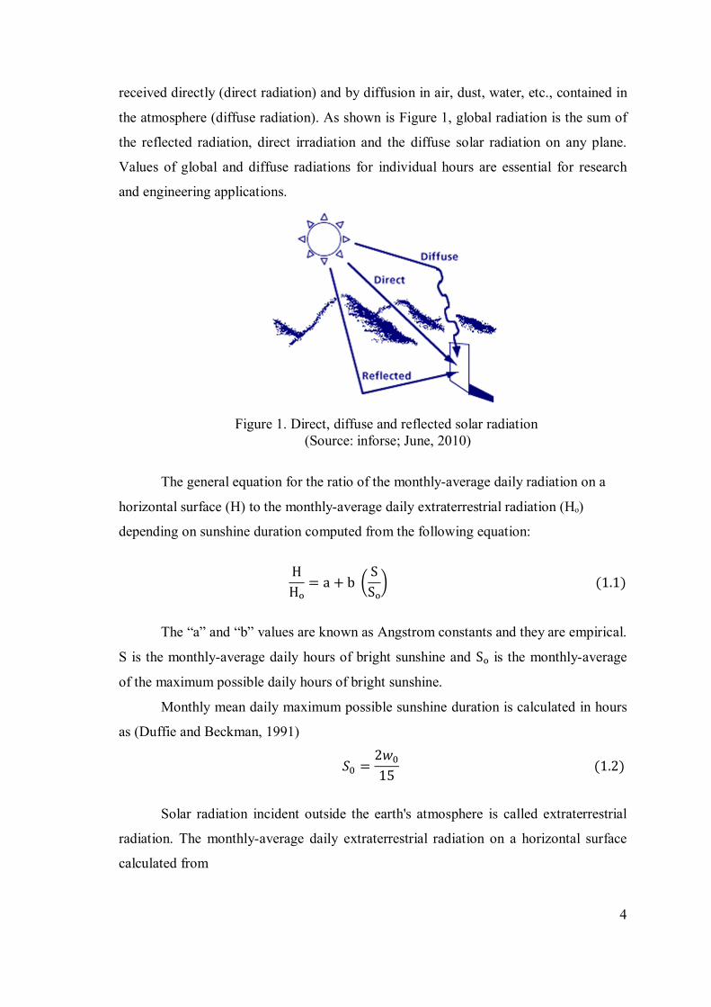
The general equation for the ratio of the monthly-average daily radiation on a
horizontal surface (H) to the monthly-average daily extraterrestrial radiation (Hₒ)
depending on sunshine duration computed from the following equation:
HHₒ = a + b
SSₒ (1.1)
The “a” and “b” values are known as Angstrom constants and they are empirical.
S is the monthly-average daily hours of bright sunshine and Sₒ is the monthly-average
of the maximum possible daily hours of bright sunshine.
Monthly mean daily maximum possible sunshine duration is calculated in hours
as (Duffie and Beckman, 1991)
푆 =2푤15 (1.2)
Solar radiation incident outside the earth's atmosphere is called extraterrestrial
radiation. The monthly-average daily extraterrestrial radiation on a horizontal surface
calculated from
5
Hₒ =24π Gₒ cosϕ cosδ sin푤 +
π180 푤 sinϕ sinδ (1.3)
where,
Gₒ = 퐺 1 + 0,033 cos360n365 (1.4)
and
훿 = 23.45 sin360(284 + 푛)
365 (1.5)
G is the solar constant (=1,367 W/m²), ϕ is the latitude of the area, δ is the
solar declination that is the angle between a plane perpendicular to a line between the
earth and the sun and the earth's axis, n is the number of the day starting from the 1st of
January and 푤 is sunset hour angle, which can be calculated from the equation as
follows:
cos 푤 = −푡푎푛휙 푡푎푛훿 (1.6)
Diffuse radiation is the second type of solar radiation. The solar radiation
received from the sun after its direction has been changed by scattering in the
atmosphere. The total radiation on a horizontal surface is recorded at a large number of
locations, while diffuse radiation, needed in many solar energy applications, is
measured in comparatively few locations. The diffuse fraction under clear-sky
conditions may be calculated theoretically. However, it is common practice for the large
number data to be condensed and presented in simple useable form obtained from the
measurements for various types of users. Correlation used for predicting monthly
average daily values of diffuse radiation may be classified in four groups as: (i) from the
clearness index (k = H/ Hₒ), (ii) from the relative sunshine duration or sunshine fraction
(S/ S ), (iii) from the diffuse coefficient (k = H / Hₒ), and (iv) from the diffuse
fraction or cloudiness index (k = H /H).
Solar energy is considered as a key source not only for the world but also for
Turkey. Turkey lies in a sunny belt between 36° and 42° N latitudes and is
geographically well situated with respect to solar energy potential. Turkey is located in
an advantageous position in Europe for the purposes of solar power. The global solar
radiation values on a horizontal surface and daily sunshine hours are measured in
Turkey by many recording stations in Turkish State Meteorological Service (DMI).
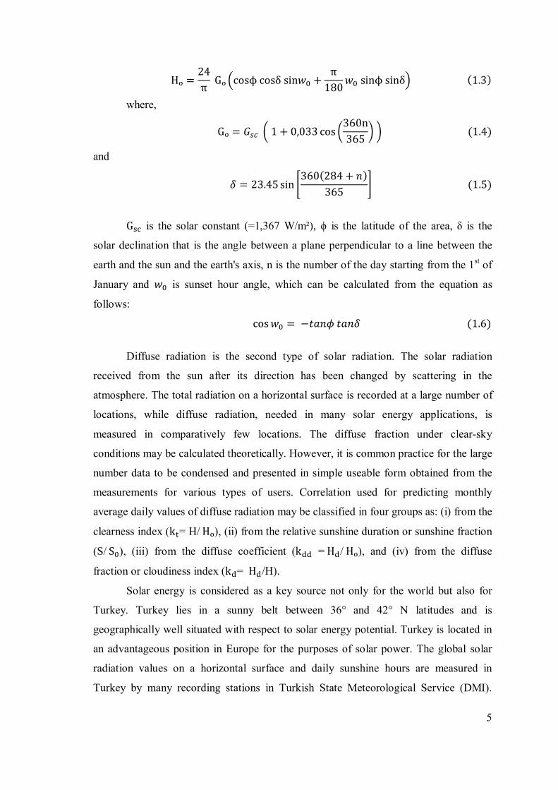
6
According to these data, Turkey's average annual total sunshine duration is
calculated as 2,640 hours (daily total is 7.2 hours), and average total radiation pressure
as 1,311 kWh/m²-year (daily total is 3.6 kWh/m²). Solar energy potential is calculated
as 380billion kWh/year. In Table 1, it can be seen that Turkey’s monthly-average solar
radiation values and sunshine duration.
Table 1. Turkey’s monthly-average solar radiation data
(Source: EIE; June,2011)
Months Monthly-average solar radiation (Kcal/cm2-month) (kWh/m2-month)
Sunshine dur. (h/month)
January 4.45 51.75 103.0 February 5.44 63.27 115.0
March 8.31 96.65 165.0 April 10.51 122.23 197.0 May 13.23 153.86 273.0 June 14.51 168.75 325.0 July 15.08 175.38 365.0
August 13.62 158.40 343.0 September 10.60 123.28 280.0
October 7.73 89.90 214.0 November 5.23 60.82 157.0 December 4.03 46.87 103.0
Total 112.74 1,311 2,640 Average 308.0 kcal/cm2-day 3.6 kWh/m2-day 7.2 h/day
The main objectives of the present study are:
To establish monthly-average daily global and diffuse radiation values for
Izmir, Turkey.
To develop new models via to the equations in the literature for Izmir.
To compare all the models by using statistical methods.
This thesis is composed of 7 chapters. In order; Chapter 1 is the introduction
part. Chapter 2 gives a brief explanation of literature survey. Chapter 3 is concerned
with the solar radiation measurements. First part is prepared for the experimental data.
Such components as pyranometer, data logger specifications are expressed one by one.
Last part is for statistical methods. Chapter 4 consists of the analysis of global solar
radiation and its models. New developed models are also mentioned in this chapter.

7
Chapter 5 is concerned with the analysis of diffuse solar radiation. In this chapter, the
study is divided into 4 groups. Each group has got three models which one of them is
the new calculated model. Chapter 6 is concerned with the calculation results of solar
energy on the horizontal surface both global and diffuse radiations. Finally, in Chapter
7, conclusions are presented.
8
CHAPTER 2
LITERATURE SURVEY
2.1. Global Solar Radiation
The estimation of daily global solar radiation has been reviewed in most of the
researches based on the duration of sunshine, identifying the best model and
determining different coefficients for several locations.
Diez-Mediavilla, et al. (2004) made an analysis of 10 arithmetic models used to
calculate diffuse solar irradiance on inclined surfaces in Valladolid, Spain. The actual
data readings were taken hourly and daily basis from the 1st of August, 1998 until the
15th of March, 2000. Three statistical methods have been used to confirm the results.
Taking the area’s feature into account was mentioned important for diffuse irradiance
on inclined surfaces. In conclusion the Muneer model and the the Reindl model gives
the best results for hourly and for daily values.
Stone (1993) proposed t- statistics as a statistical indicator for the evaluation and
comparison of solar radiation estimation models. A relationship was developed for the t-
statistic by using data published in the solar energy literature as a function of the widely
used root mean square and mean bias errors. It was shown that the use of the root mean
square and mean bias errors separately can lead to the incorrect selection. As a result,
the t-statistic method can be used in conjunction with the root mean square and mean
bias errors to more reliably assess a model's analysis.
Akpabio et al. (2004) presented a quadratic form of the Angstrom-Prescott
model to estimate global solar radiation at Onne (lat. 4°46′N, long. 7°10′E), a tropical
location. Ogelman et al. model, Akinoglu and Ecevit model, Fagbenle's model were
compared with the ones developed for the Nigerian environment. The results showed
that the relationship between clearness index and relative shine in quadratic form is to
some extent locality-dependent.
The measured data of global and diffuse solar radiation on a horizontal surface,
the number of bright sunshine hours, mean daily ambient temperature, maximum and
minimum ambient temperatures, relative humidity and amount of cloud cover for
9
Jeddah (lat. 21°42′37′′N, long. 39°11′12′′E), Saudi Arabia, during the period (1996–
2007) were analyzed by El-Sebaii et al. (2009). The monthly averages of daily values
for the meteorological variables calculated. The data were then divided into two sets.
The sub-data set 1 (1996–2004) was employed to develop empirical correlations
between the monthly average of daily global solar radiation fraction (H/Hₒ) and the
various weather parameters. The sub-data set 2 (2005–2007) were then used to evaluate
the derived correlations. The total solar radiation on horizontal surfaces was separated
into the beam and diffuses components. Empirical correlations for estimating the diffuse
solar radiation incident on horizontal surfaces have been proposed. The total solar
radiation incident on a tilted surface with different tilt angles was then calculated using
both Liu and Jordan isotropic model and Klucher’s anisotropic model. It was inferred
that the isotropic model is able to estimate the total solar radiation incident on a tilted
surface more accurate than the anisotropic one. At the optimum tilt angle, the maximum
value was obtained as 36 (MJ/m²day) during January.
A quadratic relationship between solar insolation and duration of solar radiation
data has been investigated by Aksoy (1996) in order to estimate monthly average global
irradiance for Ankara, Antalya, Samsun, Konya, Urfa and Izmir. A general quadratic
formula was found that represents the whole of Turkey. A quadratic model was chosen
because it better represents population distribution than the linear Angstrom model,
especially at extreme points. He concluded that monthly global solar irradiance can be
estimated with about 4% relative error with the quadratic formula.
Ulgen and Hepbasli (2008) used solar radiation data for Ankara (lat. 39°57’N,
long. 32°53’E, alt. 894 m), Istanbul (lat. 40°58’N, long. 29°05’E, alt. 39 m) and Izmir
(lat. 38°24’N, long. 27°10’E, alt. 15 m) of Turkey to establish a relationship between
the monthly average daily diffuse fraction and the monthly average daily diffuse
coefficient with the monthly average daily clearness index and monthly-average daily
sunshine fraction. 32 different models and 8 new models were compared due to the
widely used 8 statistical indicators. They concluded that the new models predict the
values of cloudiness index and the diffuse coefficient as a function of clearness index
and sunshine fraction for the three cities better than other available models.
Gunes (2001) examined the variation of monthly-average daily global solar
radiation in 11 stations located in 9 cities in Turkey. Five of the stations were depending
on Turkish State Meteorological Service (DMI), and the others were belonging to
10
Electrical Works Research Directorate (EIEI). Kilic and Ozturk’s model (1983),
Ogelman et al.’s model (1984) and Aksoy’s model (1997) were compared according to
the values of mean quadratic error, mean absolute error and correlation coefficient. It
has been seen that the most successful model was Ogelman et al.’s model.
Kaygusuz and Ayhan (1997) made analysis of measured solar data in the form of
hourly-average solar irradiation, monthly-average daily global solar radiation and
percentage frequency distribution in Trabzon, Turkey (lat. 41°10’N, long. 40°20’E).
The calculations were based on generally accepted equations. Due to the calculations
the hourly-average global solar radiation and hourly-average diffuse solar radiation
were plotted. They concluded that the maximum value of the monthly-average daily
global radiation was recorded in June with an amount of 21.6 MJ/m². The monthly-
average daily clearness index varied between 0.29 in March and 0.47 in June. The
highest values of hourly radiation were recorded between 11am-12am during the day.
Bakirci (2006) presented a third-order equation for the calculation of the
monthly-average daily global solar radiation for Erzurum, Turkey (lat. 39°55’N, long.
41°16’E, alt. 1869 m). Measured data taken from Turkish State Meteorological Service
for four years. Additionally for computing the monthly-average daily global solar
radiation 9 models available in the literature were used. The models were examined by
three statistical methods respectively, mean bias error (MBE), root mean square error
(RMSE), and t-statistic. It has been concluded that the lowest RMSE and MBE values
were gathered from the third-order equation model and the lowest t-statistic value is
taken from the model of Ulgen and Hepbasli. Except Tiris’ model, all used models were
appropriate for calculating the monthly-average daily global radiation in Erzurum due to
t-critic value that is 3.106.
Ogulata and Ogulata (2001) calculated the monthly-average daily and hourly
global, diffuse and direct radiations on a horizontal surface in Adana, Turkey (lat.
~37°00’N, long. ~35°20’E, alt. ~20 m). They concluded that the maximum monthly-
average daily global radiation was recorded as 18.51 MJ/m²day in July. Diffuse
radiation values range from 9.1 MJ/m²day in July to 2.8 MJ/m²day in January. The
equations used in the study were applicable for Adana for predicting global and hourly
solar radiations.
Celik (2005) analyzed the solar radiation data in Ankara,Turkey (lat. 39°95’N,
long. 32°88’E, alt. 891 m) based on 6 years of global solar radiation data measured on a
11
horizontal surface by the DMI. The yearly and monthly optimum tilt angles were
determined by converting available data. It has been concluded that the yearly total
optimal tilt angle was 39.40° for the year 2000. The smallest optimal tilt angle was 6.7°
in June and the largest was 65.2° in November.
Ulgen and Hepbasli (2004) reviewed solar radiation models for Turkey in
general and some of its provinces. 41 models used to estimate the monthly average daily
global solar radiation on a horizontal surface were categorized in four groups namely;
lineer models, polynomial or quadratic models, angular models, and modified
Angstrom-type models. They concluded that most of solar radiation models developed
for Turkey over a 19 year period was in the polynomial forms and the models gave
reasonably well results for Turkey or elsewhere with similar climatic conditions.
Aras et al. (2006) developed empirical models to predict the monthly-average
daily global solar radiation over twelve provinces in the Central Anatolia Region (CAR)
of Turkey and to compare calculated values obtained from developed models with data
measured by the Turkish State Meteorological Service (DMI) in the period from
January 1990 to December 1996 based on the various statistical methods. The general
linear, quadratic, and cubic polynomial models were derived for the region. Values for
the maximum monthly average daily measured global solar radiation ranged from 24
(for Cankiri, Turkey) and 27.10 (for Nevsehir, Turkey) to 25.85 MJ/m2. Maximum
average daily measured sunshine duration values were in the range of 9.6 (for Cankiri,
Turkey) and 11.90 (for Nevsehir and Sivas, Turkey) to 11.12 h.
Ulgen and Hepbasli (2004) compared some existing models used for estimating
the monthly-average daily global solar radiation for Istanbul, Ankara and Izmir of
Turkey. They also developed some empirical models for these cities. The MBE, RSME,
MPE, and t-statistic methods were used to evaluate the performance of the models.
They concluded that the 2 new empirical models were found to be reasonably good for
all the test methods.
A new correlation for the estimation of monthly average daily global solar
radiation was developed by Akinoglu and Ecevit (1990) and they compared with the
correlations of Rietveld, Benson et al., Ogelman et al. The overall results show that the
quadratic form gives better performance in terms of global applicability. The new
quadratic model should be preferred for the monthly average global solar radiation
estimation when the data for bright sunshine hours are available.
12
Togrul et al. (2002) developed some statistical relations in order to estimate
monthly mean daily global solar radiation in Turkey. The global solar radiation was
measured by Kipp pyranometer in 6 observation stations. Various regression analyses
were applied to estimate monthly mean solar radiation in Turkey, by using the daily
fraction of possible hours, (n/N), where n is the measured sunshine duration in a day
and N is the theoretical day length of that day. Three statistical tests, root mean square
error (RMSE) and mean bias error (MBE), and t-statistic were used to evaluate the
accuracy of the correlations. It was seen that the equations which include the summer
and winter periods gave better results than the others in all of the developed equations.
2.2. Diffuse Solar Radiation
Ulgen and Hepbasli (2001) showed the monthly-average global and diffuse solar
radiation data. The theoretical analysis of the monthly-average clearness index was
defined. As a result, the value of the monthly-average global radiation varied from 5964
kJ/m² in December to 27.154kJ/m² in June. The values of the monthly-average daily
clearness index raged from 0.45 to 0.66. The developed models were found to be
suitable and reliable. Ulgen and Hepbasli (2002) used hourly global and diffuse radiation
measurements over a 5 year period to establish a relationship between the daily diffuse
fraction and the daily clearness index for Izmir, Turkey. The comparisons of the results
were done with other correlations available in the literature. After generating the results
from 16 models, the best results were obtained from the higher order polynomial
models.
Aras et al. (2005) developed 12 new models for estimating monthly average
daily diffuse solar radiation on a horizontal surface in the CAR and the diffuse solar
radiation models in the literature were analyzed in detail. In conclusion, the provinces in
the CAR have almost the same diffuse solar radiation values.
Tarhan and Sari (2004) analyzed global and diffuse solar radiation in 5 cities in
the CBSR. A quadratic polynomial equation was empirically developed to predict the
monthly average daily global radiation. A hybrid model was also developed based on
the predictions of six existing models. As a result, the quadratic model has been chosen
as the best model for the solar radiation data of the CBSR region.
13
Jiang (2008) used nine diffuse radiation models for the daily data between
January 1, 1994 and December 31, 1998 from 16 stations all over China. Validation of 9
models for predicting monthly mean daily diffuse solar radiation has been performed by
using the statistical errors MPE, MBE and RMSE. It was found that the second degree
polynomial relationship, Iqbal model, is suitable for diffuse radiation estimation in
China. The Iqbal model works better in the eastern part of China than in the west. The
A.A. El-Sebaii model could not be used to estimate diffused radiation accurately in
China. The Liu and Jordan model could also be used for diffuse radiation estimation in
China.
An analysis of measurement for Gebze, Turkey has been done by Tiris et al.
Applying measured data correlation models for calculating the hourly and monthly
diffuse radiations were derived for nine years. As a result, the maximum value of the
monthly-average daily global radiation was 24 MJ/m² in June. And the minimum value
was 2.2 MJ/m² recorded in December.
Ahmad and Tiwari (2009) reviewed solar radiation models for predicting the
average daily and hourly global radiation, beam radiation and diffuse radiation on
horizontal surface. It was observed that Collares-Pereira and Rabl model as modified by
Gueymard (CPRG) yielded the best performance for estimating mean hourly global
radiation incident on a horizontal surface in India. Estimations of monthly average
hourly beam and diffuse radiation are discussed. It was observed that Singh-Tiwari and
Jamil-Tiwari models generally give better results for climatic conditions of India. Fifty
models using the Angstrom–Prescott equation to predict the average daily global
radiation with hours of sunshine are considered. It was reported that Ertekin and Yaldiz
model showed the best performance against measured data of Konya, Turkey.
Ulgen and Hepbasli (2008) developed 8 new models for estimating the monthly
average daily diffuse solar radiation on a horizontal surface in three big cites of Turkey.
The new models are then compared with the 32 models available in the literature in
terms of the widely used statistical indicators. It may be concluded that the new models
predict the values of cloudiness index and diffuse coefficient as a function of clearness
index and sunshine fraction for three big cities in Turkey better than other available
models.
Che et al. (2010) used forty years of daily global and diffuse radiation data to
characterize the atmospheric conditions at 14 stations in China. These sites are located

14
so widely throughout China that they can be considered representative of different
climatic regions of China. Two polynomial models have been developed to simulate
clearness index and diffuse ratio at each station and also they proposed a trigonometric
model in conjunction with a sine and cosine wave for estimating daily global solar
radiation. The statistical estimator of root mean square (RMSE) showed that the
developed models are suitable for simulations of clearness index and diffuse ratio at
most premium solar radiation stations in China.
.
15
CHAPTER 3
EXPERIMENTAL SOLAR RADIATION DATA AND
STATISTICAL METHODS
3.1. Experimental Data
The experimental set-up is located at the Mechanical Engineering Department in
Izmir Institute of Technology. Its latitude and longitude are 38°42’N, 27°12’E,
respectively.
Pyranometers are used for measuring global radiation data. Through these
instruments most of the available data on solar radiation are obtained. A pyranometer
produces voltages from the thermopile detectors that are a function of the incident
radiation. It is necessary to use a potentiometer to detect and record this output.
Radiation data usually must be integrated over some period of time, such as an hour or a
day.
Two additional kinds of measurements are made with pyranometers;
measurements of diffuse radiation on horizontal surfaces and measurements of solar
radiation on inclined surfaces.
In this study, the global radiation on a horizontal surface was measured at an
interval of 10 minute by using a Kipp-Zonen pyranometer (Model CM11) during the
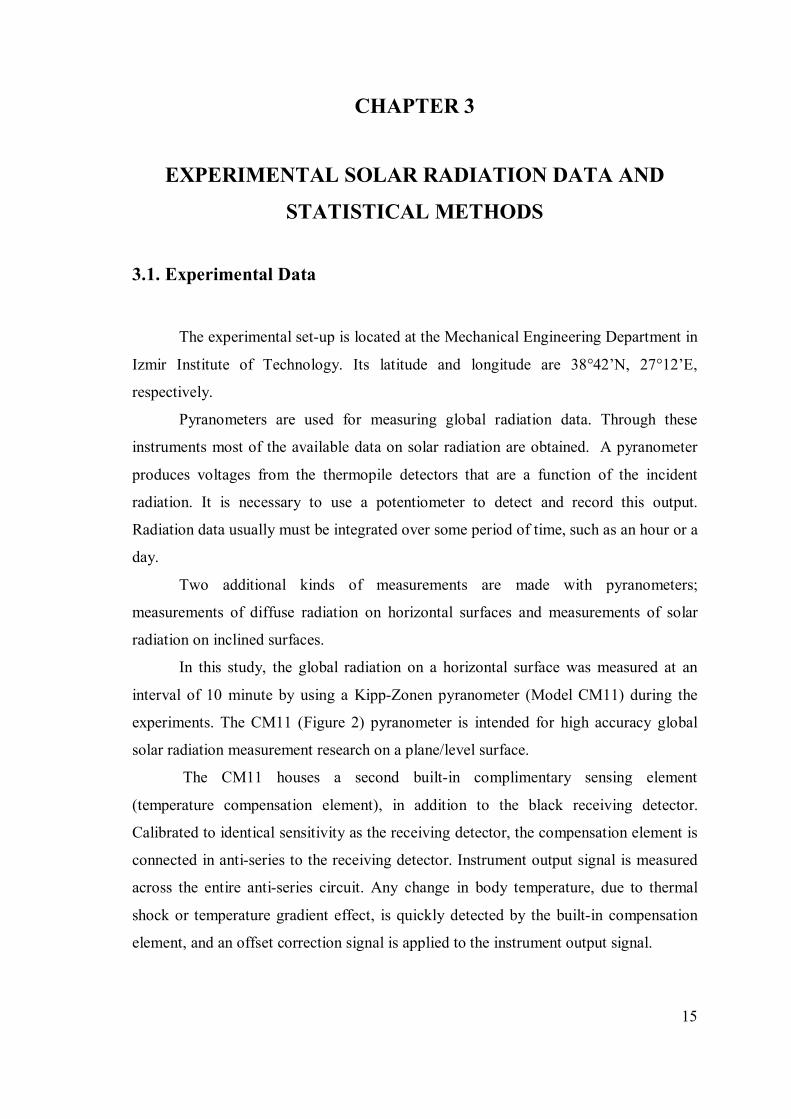
experiments. The CM11 (Figure 2) pyranometer is intended for high accuracy global
solar radiation measurement research on a plane/level surface.
The CM11 houses a second built-in complimentary sensing element
(temperature compensation element), in addition to the black receiving detector.
Calibrated to identical sensitivity as the receiving detector, the compensation element is
connected in anti-series to the receiving detector. Instrument output signal is measured
across the entire anti-series circuit. Any change in body temperature, due to thermal
shock or temperature gradient effect, is quickly detected by the built-in compensation
element, and an offset correction signal is applied to the instrument output signal.
16
Figure 2. Approximate construction of CM11 (Source: Kipp-Zonen, 2010)
Table 2. CM11 specfications (Source: Kipp-Zonen, 2010)
Spectral range 305-2800 nm
Sensitivity 5.14 uV/W/m2
Internal resistance 700-1500 Ohms
Response time 15 s
Nonlinearity <+0.6% (<1000W/m2) Zero offset +7 W/m2
ISO-9060 Class Secondary Standard
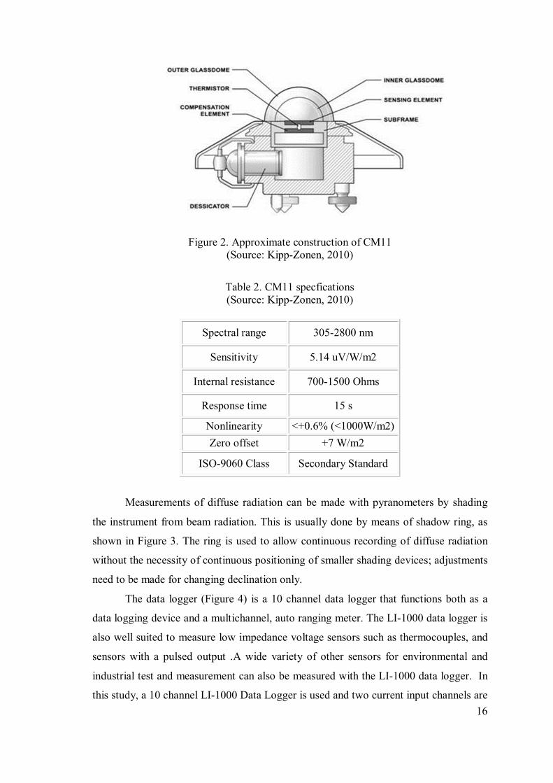
Measurements of diffuse radiation can be made with pyranometers by shading
the instrument from beam radiation. This is usually done by means of shadow ring, as
shown in Figure 3. The ring is used to allow continuous recording of diffuse radiation
without the necessity of continuous positioning of smaller shading devices; adjustments
need to be made for changing declination only.
The data logger (Figure 4) is a 10 channel data logger that functions both as a
data logging device and a multichannel, auto ranging meter. The LI-1000 data logger is
also well suited to measure low impedance voltage sensors such as thermocouples, and
sensors with a pulsed output .A wide variety of other sensors for environmental and
industrial test and measurement can also be measured with the LI-1000 data logger. In
this study, a 10 channel LI-1000 Data Logger is used and two current input channels are
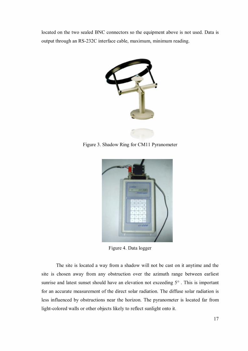
17
located on the two sealed BNC connectors so the equipment above is not used. Data is
output through an RS-232C interface cable, maximum, minimum reading.
Figure 3. Shadow Ring for CM11 Pyranometer
Figure 4. Data logger
The site is located a way from a shadow will not be cast on it anytime and the
site is chosen away from any obstruction over the azimuth range between earliest
sunrise and latest sunset should have an elevation not exceeding 5° . This is important
for an accurate measurement of the direct solar radiation. The diffuse solar radiation is
less influenced by obstructions near the horizon. The pyranometer is located far from
light-colored walls or other objects likely to reflect sunlight onto it.
18
Meteorological data including temperature, relative humidity, global solar
radiation, and precipitation etc. for Izmir Institute of Technology (IZTECH) have been
recorded since 2005. Solar radiation data were compiled from IZTECH Meteorological
Station in Figure-3 from February, 2005 to May, 2007. It was over a period of 821 days,
and 116,101 for 10-minute values. On the other hand, the diffuse solar radiation data
that is used in the study have been recorded from February, 2004 to December, 2005.
3.2. Statistical Methods
In the literature, there are several statistical test methods used to statistically
evaluate the performance of the models of solar radiation estimations. Among these,
correlation mean bias error (MBE), root mean square error (RMSE), and the t-statistic
(t-stat) errors are the most widely used ones.
3.2.1. Mean Bias Error
The mean bias error (MBE) provides information on the long-term performance
of the correlations by allowing a comparison of the actual deviation between calculated
and measured values term by term. The ideal value of the MBE is zero. The MBE is
given by,
MBE = y − x (3.1)
where, y is the kth calculated value, x is the kth measured value, and n is the total
number of observations.
3.2.2. Root Mean Square Error
The root-mean-square error (RMSE) is a frequently used measure of the
differences between values predicted by a model or an estimator and the values actually
observed from the thing being modeled or estimated. RMSE is a good measure of
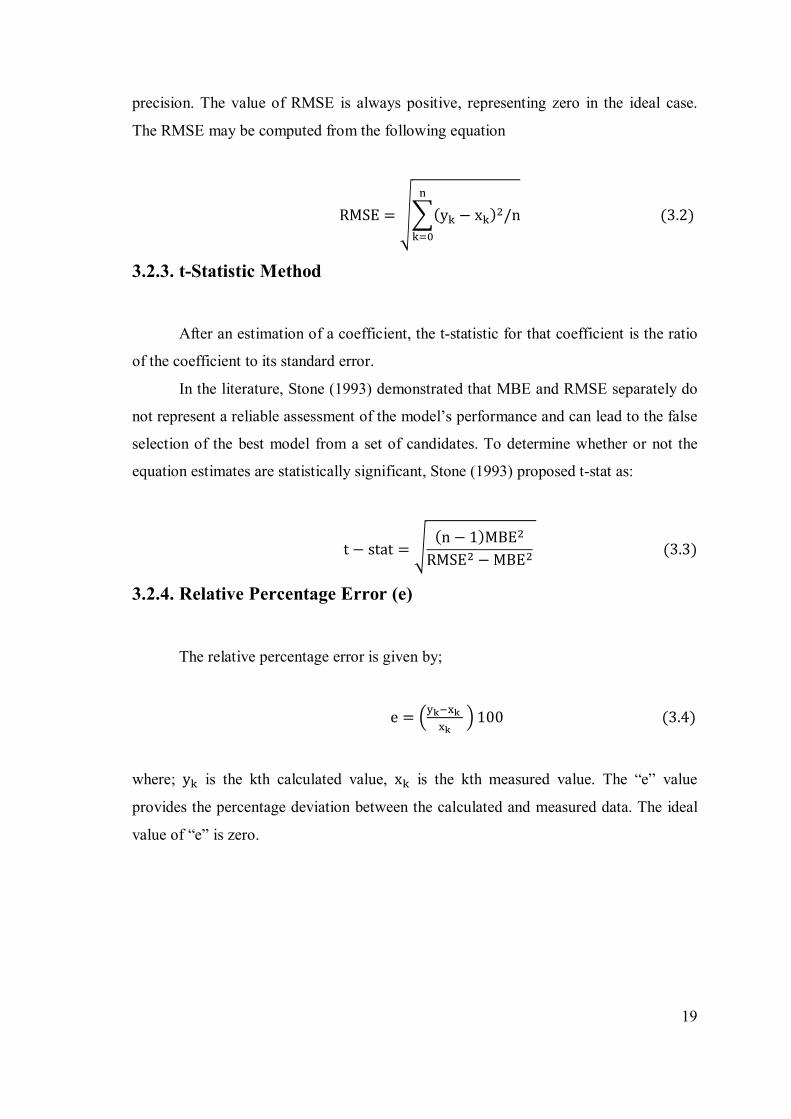
19
precision. The value of RMSE is always positive, representing zero in the ideal case.
The RMSE may be computed from the following equation
RMSE = (y − x ) /n (3.2)
3.2.3. t-Statistic Method
After an estimation of a coefficient, the t-statistic for that coefficient is the ratio
of the coefficient to its standard error.
In the literature, Stone (1993) demonstrated that MBE and RMSE separately do
not represent a reliable assessment of the model’s performance and can lead to the false
selection of the best model from a set of candidates. To determine whether or not the
equation estimates are statistically significant, Stone (1993) proposed t-stat as:
t − stat =(n − 1)MBE
RMSE − MBE (3.3)
3.2.4. Relative Percentage Error (e)
The relative percentage error is given by;
e = 100 (3.4)
where; y is the kth calculated value, x is the kth measured value. The “e” value
provides the percentage deviation between the calculated and measured data. The ideal
value of “e” is zero.
20
CHAPTER 4
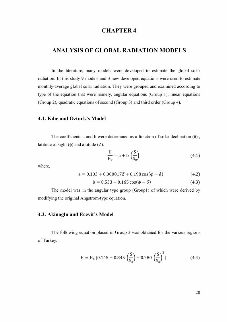
ANALYSIS OF GLOBAL RADIATION MODELS
In the literature, many models were developed to estimate the global solar
radiation. In this study 9 models and 3 new developed equations were used to estimate
monthly-average global solar radiation. They were grouped and examined according to
type of the equation that were namely, angular equations (Group 1), linear equations
(Group 2), quadratic equations of second (Group 3) and third order (Group 4).
4.1. Kılıc and Ozturk’s Model
The coefficients a and b were determined as a function of solar declination (δ) ,
latitude of sight (ϕ) and altitude (Z).
HHₒ = a + b
SSₒ (4.1)
where,
a = 0.103 + 0.000017푍 + 0.198 cos(휙 − 훿) (4.2)
b = 0.533 + 0.165 cos(휙 − 훿) (4.3)
The model was in the angular type group (Group1) of which were derived by
modifying the original Angstrom-type equation.
4.2. Akinoglu and Ecevit’s Model
The following equation placed in Group 3 was obtained for the various regions
of Turkey.
H = Hₒ [0.145 + 0.845 SSₒ − 0.280
SSₒ ] (4.4)
21
4.3. Tasdemiroglu and Sever’s Model
A second order polynomial equation for Turkey’s general was formulated as:
H = Hₒ [0.195 + 0.676 SSₒ − 0.142
SSₒ ] (4.5)
4.4. Oz’s Model (1997)
For the whole of Turkey, Oz obtained a general equation from Group 3 by using
data measured at 9 stations. It was as follows:
H = Hₒ [0.3420 + 0.5002 SSₒ − 0.1014
SSₒ ] (4.6)
4.5. Aksoy’s Model
Aksoy developed a second order quadratic equation (Group 3) in order to
calculate monthly-average global irradiance for 6 places in Turkey, as follows:
H = Hₒ [0.148 + 0.668 SSₒ − 0.079
SSₒ ] (4.7)
4.6. Ulgen and Ozbalta’s Model
The following equation is belonged to Group 3 and it is estimated for Izmir,
Turkey.
H = Hₒ [0.0959 + 0.9958SSₒ − 0.3922
SSₒ ] (4.8)
4.7. Togrul and Togrul’s Model
Togrul et al. obtained below mentioned equation for Ankara, Antalya, Izmir,
Aydin, Adana and Elazig to estimate monthly-average global solar radiation.
22
The equation was in the Group 2.
HHₒ = 0.318 + 0.449
SSₒ (4.9)
4.8. Ulgen and Hepbasli’s Model
Based on measurements made in the Meteorological Station of Solar Institute,
Ege University, Izmir from 1994 to 1998, a third order quadratic equation (Group 4) is
developed. The formula is given by,
H = Hₒ [0.2408 + 0.3625 SSₒ + 0.4597
SSₒ − 0.3708
SSₒ ] (4.10)
4.9. Ulgen and Hepbasli’s Model
Using the data available for Ankara, Istanbul and Izmir over a 19-yr period,
Ulgen and Hepbasli developed the following equation:
H = Hₒ [0.2854 + 0.2591 SSₒ + 0.6171
SSₒ − 0.4837
SSₒ ] (4.11)
4.10. New Developed Equation 1
A linear equation has been developed to estimate monthly-average daily global
solar radiation in Izmir, as follows:
H = Hₒ[0.263 + 0.512 SSₒ ] (4.12)
4.11. New Developed Equation 2
Using regional data, a Group-3 type of equation has been developed that was
given by;
H = Hₒ [0.238 + 0.610SSₒ − 0.085
SSₒ ] (4.13)
23
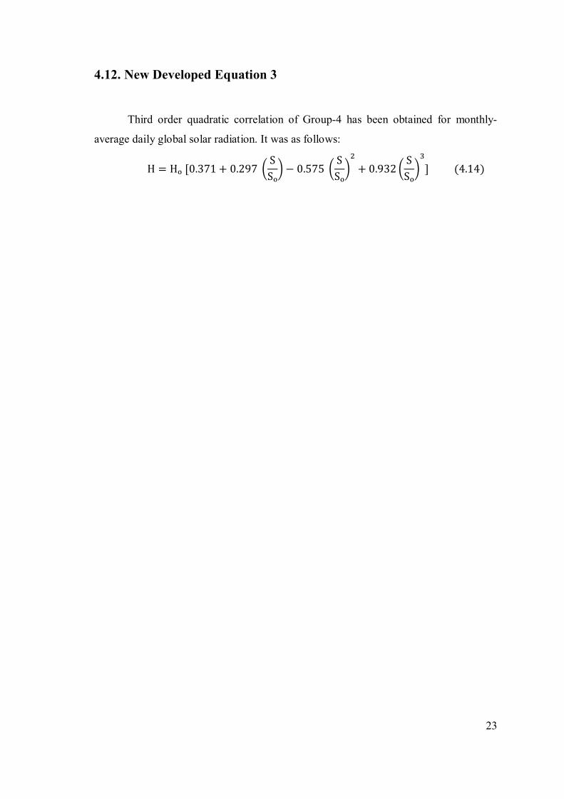
4.12. New Developed Equation 3
Third order quadratic correlation of Group-4 has been obtained for monthly-
average daily global solar radiation. It was as follows:
H = Hₒ [0.371 + 0.297 SSₒ − 0.575
SSₒ + 0.932
SSₒ ] (4.14)
24
CHAPTER 5
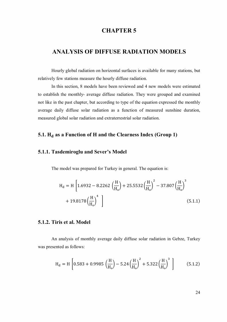
ANALYSIS OF DIFFUSE RADIATION MODELS
Hourly global radiation on horizontal surfaces is available for many stations, but
relatively few stations measure the hourly diffuse radiation.
In this section, 8 models have been reviewed and 4 new models were estimated
to establish the monthly- average diffuse radiation. They were grouped and examined
not like in the past chapter, but according to type of the equation expressed the monthly
average daily diffuse solar radiation as a function of measured sunshine duration,
measured global solar radiation and extraterrestrial solar radiation.
5.1. 퐇퐝 as a Function of H and the Clearness Index (Group 1)
5.1.1. Tasdemiroglu and Sever’s Model
The model was prepared for Turkey in general. The equation is:
H = H 1.6932 − 8.2262 HHₒ + 25.5532
HHₒ − 37.807
HHₒ
+ 19.8178HHₒ (5.1.1)
5.1.2. Tiris et al. Model
An analysis of monthly average daily diffuse solar radiation in Gebze, Turkey
was presented as follows:
H = H 0.583 + 0.9985 HHₒ − 5.24
HHₒ + 5.322
HHₒ (5.1.2)
25
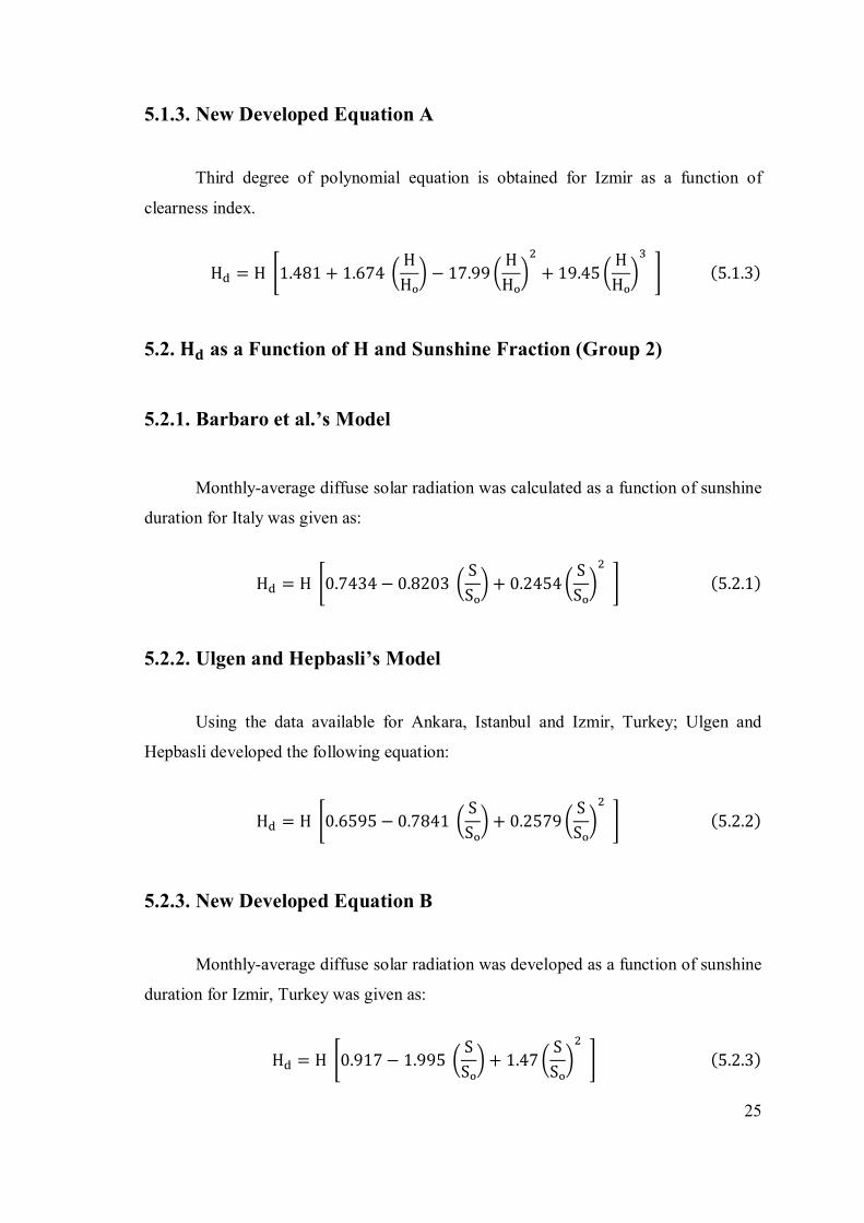
5.1.3. New Developed Equation A
Third degree of polynomial equation is obtained for Izmir as a function of
clearness index.
H = H 1.481 + 1.674 HHₒ − 17.99
HHₒ + 19.45
HHₒ (5.1.3)
5.2. 퐇퐝 as a Function of H and Sunshine Fraction (Group 2)
5.2.1. Barbaro et al.’s Model
Monthly-average diffuse solar radiation was calculated as a function of sunshine
duration for Italy was given as:
H = H 0.7434 − 0.8203 SSₒ + 0.2454
SSₒ (5.2.1)
5.2.2. Ulgen and Hepbasli’s Model
Using the data available for Ankara, Istanbul and Izmir, Turkey; Ulgen and
Hepbasli developed the following equation:
H = H 0.6595 − 0.7841 SSₒ + 0.2579
SSₒ (5.2.2)
5.2.3. New Developed Equation B
Monthly-average diffuse solar radiation was developed as a function of sunshine
duration for Izmir, Turkey was given as:
H = H 0.917 − 1.995 SSₒ + 1.47
SSₒ (5.2.3)
26
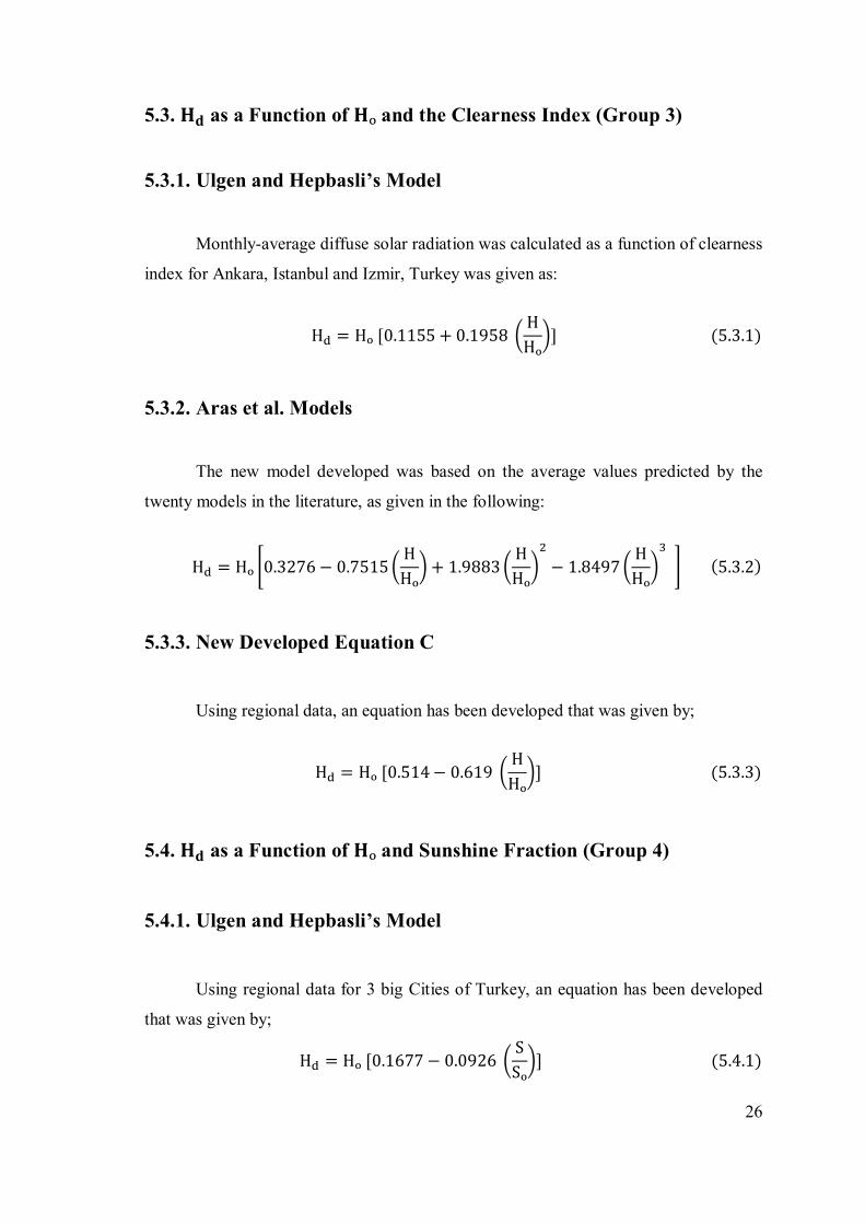
5.3. 퐇퐝 as a Function of 퐇ₒ and the Clearness Index (Group 3)
5.3.1. Ulgen and Hepbasli’s Model
Monthly-average diffuse solar radiation was calculated as a function of clearness
index for Ankara, Istanbul and Izmir, Turkey was given as:
H = Hₒ [0.1155 + 0.1958 HHₒ ] (5.3.1)
5.3.2. Aras et al. Models
The new model developed was based on the average values predicted by the
twenty models in the literature, as given in the following:
H = Hₒ 0.3276 − 0.7515HHₒ + 1.9883
HHₒ − 1.8497
HHₒ (5.3.2)
5.3.3. New Developed Equation C
Using regional data, an equation has been developed that was given by;
H = Hₒ [0.514 − 0.619 HHₒ ] (5.3.3)
5.4. 퐇퐝 as a Function of 퐇ₒ and Sunshine Fraction (Group 4)
5.4.1. Ulgen and Hepbasli’s Model
Using regional data for 3 big Cities of Turkey, an equation has been developed
that was given by;
H = Hₒ [0.1677 − 0.0926 SSₒ ] (5.4.1)
27
5.4.2. Aras et al. Model
Monthly-average diffuse solar radiation was calculated as a function of clearness
index for CAR of Turkey was given as:
H = Hₒ 0.2427 − 0.0933SSₒ + 0.1846
SSₒ − 0.2184
SSₒ (5.4.2)
5.4.3. New Developed Equation D
The model was developed for Izmir, Turkey. The equation is:
H = Hₒ 0.391 − 0.59SSₒ + 0.318
SSₒ (5.4.3)
28
CHAPTER 6
RESULTS
6.1. Results for Global Solar Radiation
In the analysis, the data measured at the IZTECH Campus between 2005 and
2007 were used. The equations mentioned in Chapter 1 were calculated in order to
estimate the total monthly-average daily global radiation.
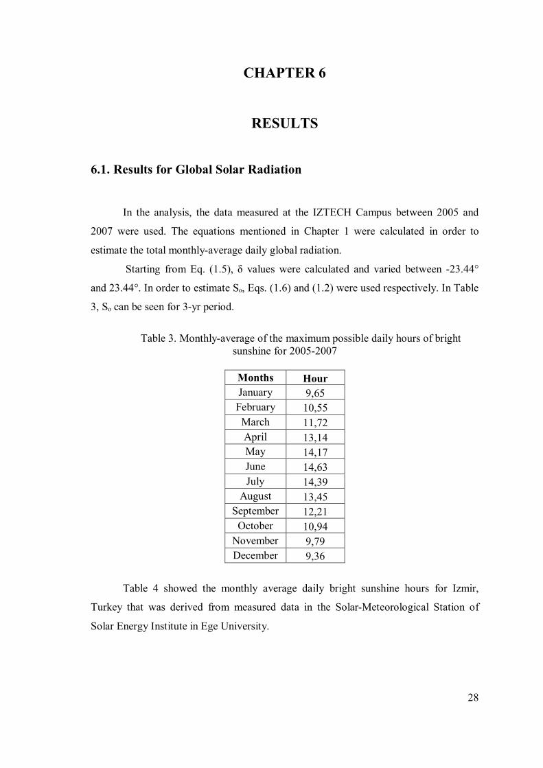
Starting from Eq. (1.5), δ values were calculated and varied between -23.44°
and 23.44°. In order to estimate Sₒ, Eqs. (1.6) and (1.2) were used respectively. In Table
3, Sₒ can be seen for 3-yr period.
Table 3. Monthly-average of the maximum possible daily hours of bright
sunshine for 2005-2007
Months Hour January 9,65 February 10,55
March 11,72 April 13,14 May 14,17 June 14,63 July 14,39
August 13,45 September 12,21
October 10,94 November 9,79 December 9,36
Table 4 showed the monthly average daily bright sunshine hours for Izmir,
Turkey that was derived from measured data in the Solar-Meteorological Station of
Solar Energy Institute in Ege University.
29
Table 4. Average of bright sunshine hours for 2005-2007 (Source: Correspondence with Assist. Prof. Dr. Koray Ülgen)
Months hour January 3,10 February 4,46
March 6,45 April 6,63 May 8,82 June 10,41 July 12,01
August 10,25 September 9,13
October 7,49 November 4,90 December 3,52
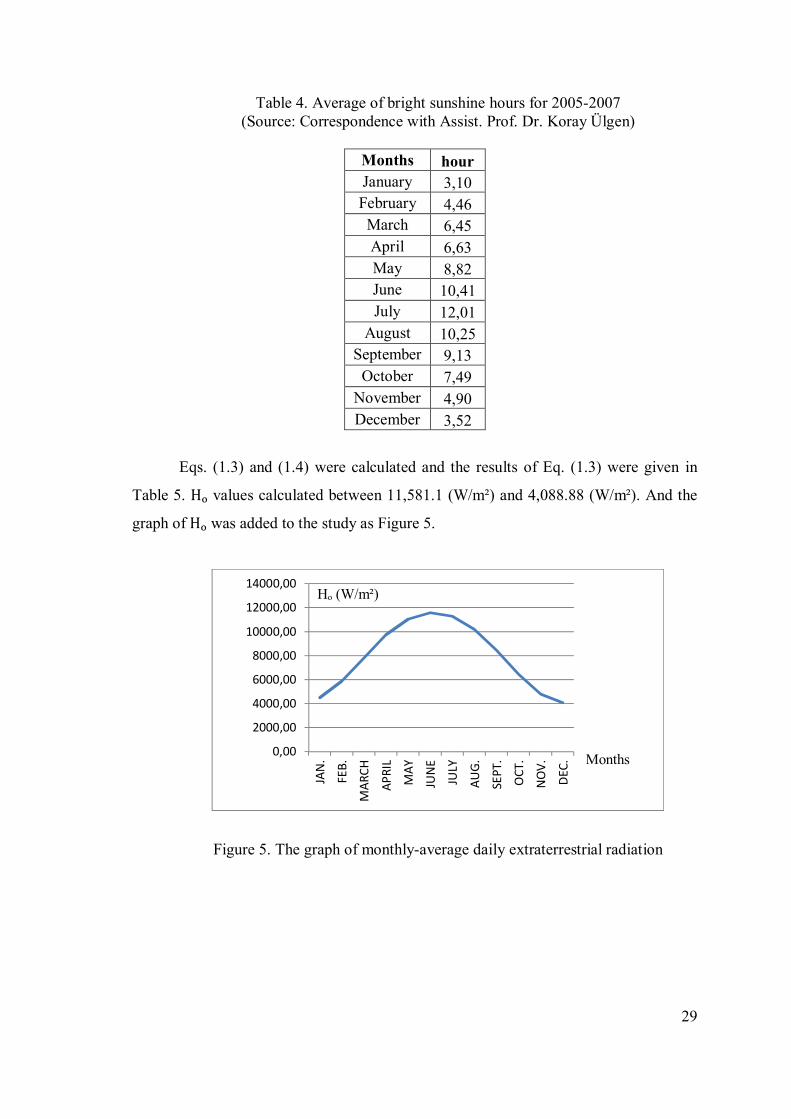
Eqs. (1.3) and (1.4) were calculated and the results of Eq. (1.3) were given in
Table 5. Hₒ values calculated between 11,581.1 (W/m²) and 4,088.88 (W/m²). And the
graph of Hₒ was added to the study as Figure 5.
Figure 5. The graph of monthly-average daily extraterrestrial radiation
0,00
2000,00
4000,00
6000,00
8000,00
10000,00
12000,00
14000,00
JAN
.
FEB.
MAR
CH
APRI
L
MAY
JUN
E
JULY
AUG.
SEPT
.
OCT
.
NO
V.
DEC. Months
Hₒ (W/m²)
30
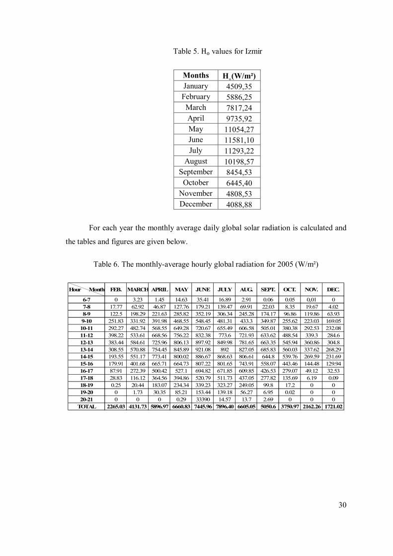
Table 5. Hₒ values for Izmir
Months H˳(W/m²) January 4509,35 February 5886,25
March 7817,24 April 9735,92 May 11054,27 June 11581,10 July 11293,22
August 10198,57 September 8454,53
October 6445,40 November 4808,53 December 4088,88
For each year the monthly average daily global solar radiation is calculated and
the tables and figures are given below.
Table 6. The monthly-average hourly global radiation for 2005 (W/m²)
Hour Month FEB. MARCH APRIL MAY JUNE JULY AUG. SEPT. OCT. NOV. DEC.
6-7 0 3.23 1.45 14.63 35.41 16.89 2.91 0.06 0.05 0,01 07-8 17.77 62.92 46.87 127.76 179.21 139.47 69.91 22.03 8.35 19.67 4.028-9 122.5 198.29 221.63 285.82 352.19 306.34 245.28 174.17 96.86 119.86 63.939-10 251.83 331.92 391.98 468.55 548.45 481.31 433.3 349.87 255.62 223.03 169.0510-11 292.27 482.74 568.55 649.28 720.67 655.49 606.58 505.01 380.38 292.53 232.0811-12 398.22 533.61 668.56 756.22 832.38 773.6 721.93 633.62 488.54 339.3 284.612-13 383.44 584.61 725.96 806.13 897.92 849.98 781.65 663.35 545.94 360.86 304.813-14 308.55 570.88 754.45 845.89 921.08 892 827.05 685.83 560.03 337.62 268.2914-15 193.55 551.17 773.41 800.02 886.67 868.63 806.61 644.8 539.76 269.59 231.6915-16 179.91 401.68 665.71 664.73 807.22 801.65 743.91 558.07 443.46 144.48 129.9416-17 87.91 272.39 500.42 527.1 694.82 671.85 609.85 426.53 279.07 49.12 32.5317-18 28.83 116.12 364.56 394.86 520.79 511.73 437.05 277.82 135.69 6.19 0.0918-19 0.25 20.44 183.07 234.34 339.23 323.27 249.05 99.8 17.2 0 019-20 0 1.73 30.35 85.21 153.44 139.18 56.27 6.95 0.02 0 020-21 0 0 0 0.29 33390 14.57 13.7 2.69 0 0 0
TOTAL 2265.03 4131.73 5896.97 6660.83 7445.96 7896.40 6605.05 5050.6 3750.97 2162.26 1721.02
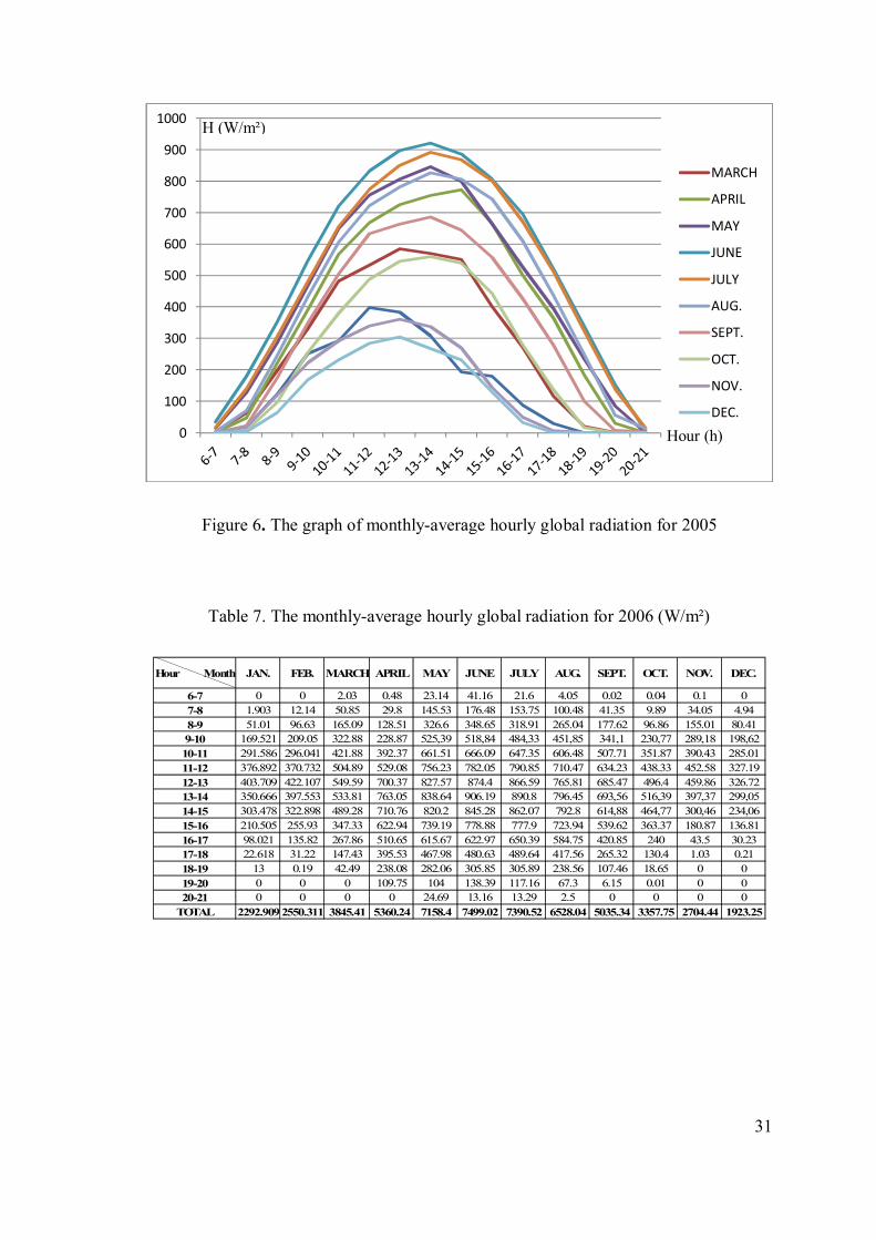
31
Figure 6. The graph of monthly-average hourly global radiation for 2005
Table 7. The monthly-average hourly global radiation for 2006 (W/m²)
0
100
200
300
400
500
600
700
800
900
1000
MARCH
APRIL
MAY
JUNE
JULY
AUG.
SEPT.
OCT.
NOV.
DEC.
Hour (h)
H (W/m²)
Hour Month JAN. FEB. MARCH APRIL MAY JUNE JULY AUG. SEPT. OCT. NOV. DEC.
6-7 0 0 2.03 0.48 23.14 41.16 21.6 4.05 0.02 0.04 0.1 07-8 1.903 12.14 50.85 29.8 145.53 176.48 153.75 100.48 41.35 9.89 34.05 4.948-9 51.01 96.63 165.09 128.51 326.6 348.65 318.91 265.04 177.62 96.86 155.01 80.419-10 169.521 209.05 322.88 228.87 525,39 518,84 484,33 451,85 341,1 230,77 289,18 198,6210-11 291.586 296.041 421.88 392.37 661.51 666.09 647.35 606.48 507.71 351.87 390.43 285.0111-12 376.892 370.732 504.89 529.08 756.23 782.05 790.85 710.47 634.23 438.33 452.58 327.1912-13 403.709 422.107 549.59 700.37 827.57 874.4 866.59 765.81 685.47 496.4 459.86 326.7213-14 350.666 397.553 533.81 763.05 838.64 906.19 890.8 796.45 693,56 516,39 397,37 299,0514-15 303.478 322.898 489.28 710.76 820.2 845.28 862.07 792.8 614,88 464,77 300,46 234,0615-16 210.505 255.93 347.33 622.94 739.19 778.88 777.9 723.94 539.62 363.37 180.87 136.8116-17 98.021 135.82 267.86 510.65 615.67 622.97 650.39 584.75 420.85 240 43.5 30.2317-18 22.618 31.22 147.43 395.53 467.98 480.63 489.64 417.56 265.32 130.4 1.03 0.2118-19 13 0.19 42.49 238.08 282.06 305.85 305.89 238.56 107.46 18.65 0 019-20 0 0 0 109.75 104 138.39 117.16 67.3 6.15 0.01 0 020-21 0 0 0 0 24.69 13.16 13.29 2.5 0 0 0 0
TOTAL 2292.909 2550.311 3845.41 5360.24 7158.4 7499.02 7390.52 6528.04 5035.34 3357.75 2704.44 1923.25
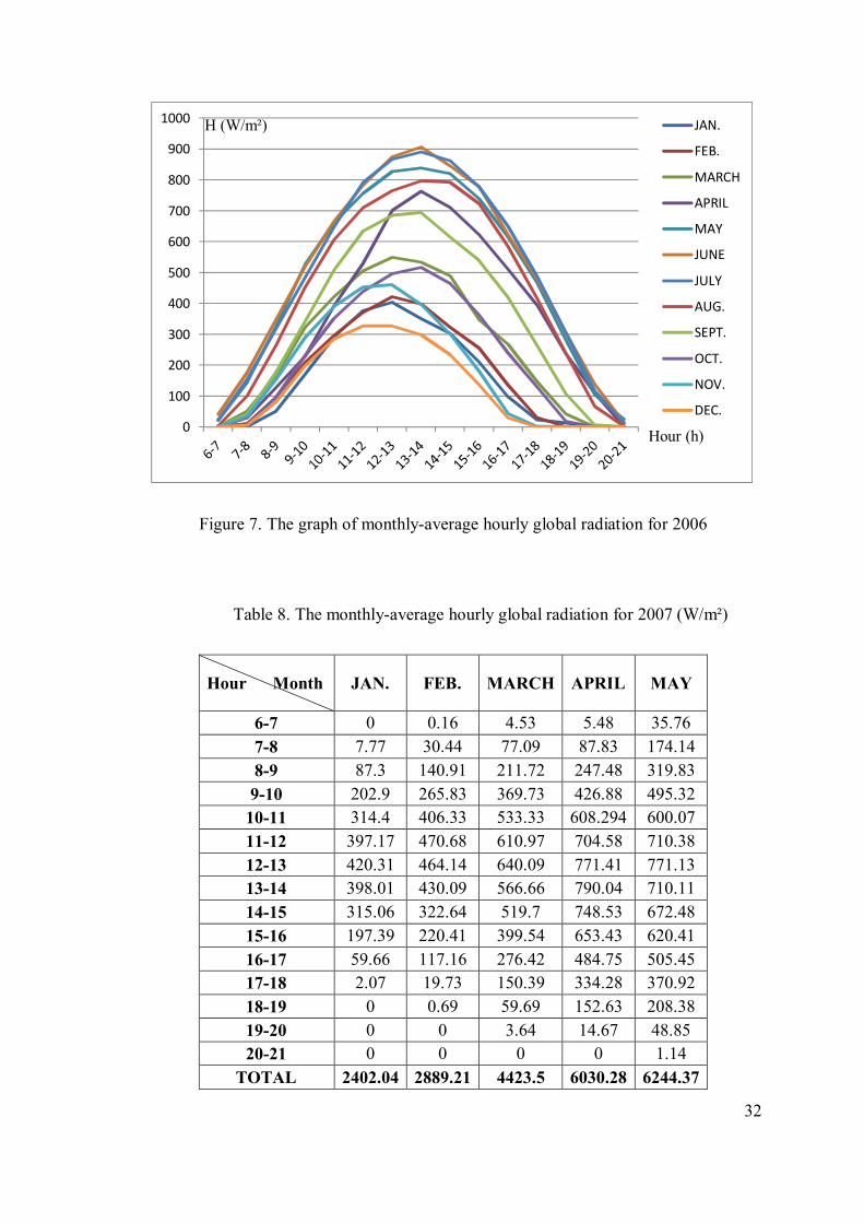
32
Figure 7. The graph of monthly-average hourly global radiation for 2006
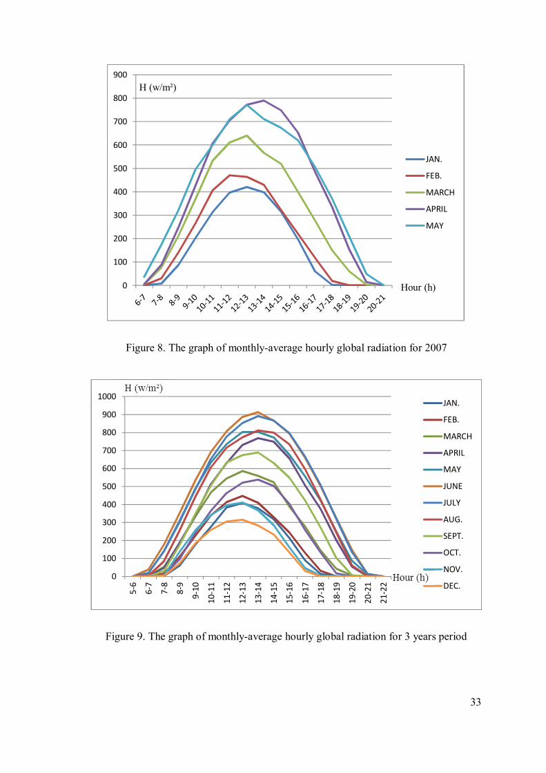
Table 8. The monthly-average hourly global radiation for 2007 (W/m²)
Hour Month JAN. FEB. MARCH APRIL MAY
6-7 0 0.16 4.53 5.48 35.76 7-8 7.77 30.44 77.09 87.83 174.14 8-9 87.3 140.91 211.72 247.48 319.83 9-10 202.9 265.83 369.73 426.88 495.32
10-11 314.4 406.33 533.33 608.294 600.07 11-12 397.17 470.68 610.97 704.58 710.38 12-13 420.31 464.14 640.09 771.41 771.13 13-14 398.01 430.09 566.66 790.04 710.11 14-15 315.06 322.64 519.7 748.53 672.48 15-16 197.39 220.41 399.54 653.43 620.41 16-17 59.66 117.16 276.42 484.75 505.45 17-18 2.07 19.73 150.39 334.28 370.92 18-19 0 0.69 59.69 152.63 208.38 19-20 0 0 3.64 14.67 48.85 20-21 0 0 0 0 1.14
TOTAL 2402.04 2889.21 4423.5 6030.28 6244.37
0
100
200
300
400
500
600
700
800
900
1000 JAN.
FEB.
MARCH
APRIL
MAY
JUNE
JULY
AUG.
SEPT.
OCT.
NOV.
DEC.
Hour (h)
H (W/m²)
33
Figure 8. The graph of monthly-average hourly global radiation for 2007
Figure 9. The graph of monthly-average hourly global radiation for 3 years period
0
100
200
300
400
500
600
700
800
900
JAN.
FEB.
MARCH
APRIL
MAY
Hour (h)
H (w/m²)
0
100
200
300
400
500
600
700
800
900
1000
5-6
6-7
7-8
8-9
9-10
10-1
1
11-1
2
12-1
3
13-1
4
14-1
5
15-1
6
16-1
7
17-1
8
18-1
9
19-2
0
20-2
1
21-2
2
JAN.
FEB.
MARCH
APRIL
MAY
JUNE
JULY
AUG.
SEPT.
OCT.
NOV.
DEC.
34
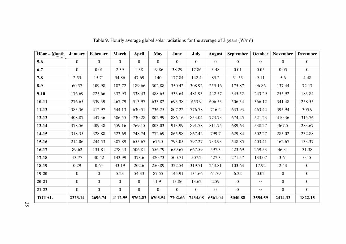
According to Table 9 the maximum value of the monthly-average daily global
radiation for the average of 2005, 2006 and 2007 was recorded to be 7,702.66W/m² in
June. The minimum value of H was 1,822.15W/m² observed during December. The
highest value was recorded between 13 -14 pm. The graph for the average of the 3 years
was shown in Figure 9. As for each month, the monthly-average hourly global solar
radiation tables were attached in Appendix A.
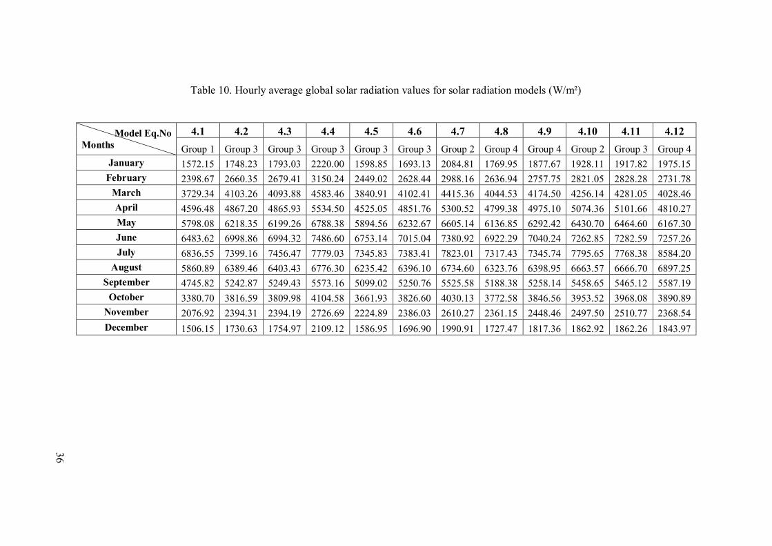
The models used to estimate the monthly-average daily global radiation on a
horizontal surface (H) were categorized in 4 groups, as seen from Eq. (4.1) to Eq.
(4.14). These groups consisted of the relations gained from Angstrom-type equations.
The types of the models and the calculated results were illustrated below in Table 10.
The regression coefficients “a and b” of the Angstrom-type correlation for the monthly
average daily global solar radiation of Eq. (4.2) and Eq. (4.3) were determined as given
in Table 11.
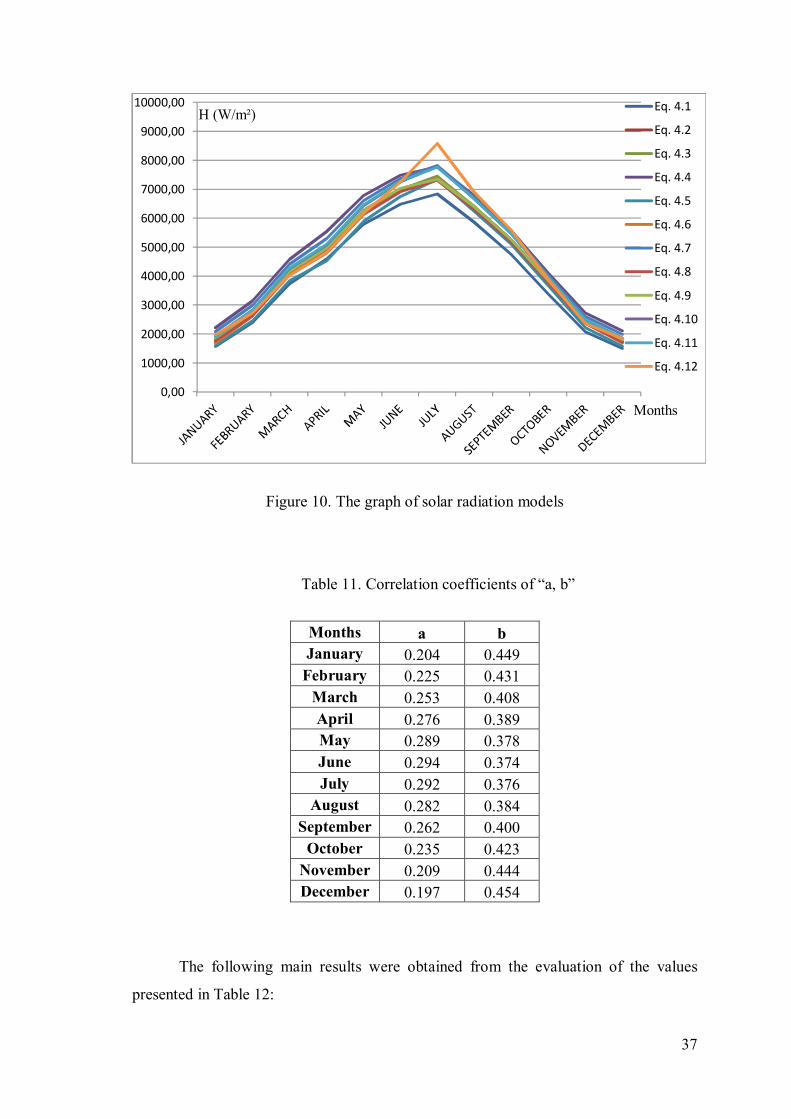
The comparison of solar radiation models can be seen in Figure 10. The results
are close to each other. To analyze the comparison in detail, statistical equations have
been referred. Values of MBE, RMSE and t-stat of selected models were shown in
Table 12. The error percentages of the models were also added in the table.
35
Table 9. Hourly average global solar radiations for the average of 3 years (W/m²)
Hour Month January February March April May June July August September October November December
5-6 0 0 0 0 0 0 0 0 0 0 0 0
6-7 0 0.01 2.39 1.38 19.86 38.29 17.86 3.48 0.01 0.05 0.05 0
7-8 2.55 15.71 54.86 47.69 140 177.84 142.4 85.2 31.53 9.11 5.6 4.48
8-9 60.37 109.98 182.72 189.66 302.88 350.42 308.92 255.16 175.87 96.86 137.44 72.17
9-10 176.69 225.66 332.93 338.43 488.65 533.64 481.93 442.57 345.52 243.29 255.92 183.84
10-11 276.65 339.39 467.79 513.97 633.82 693.38 653.9 606.53 506.34 366.12 341.48 258.55
11-12 383.36 412.97 544.13 630.51 736.25 807.22 776.78 716.2 633.93 463.44 395.94 305.9
12-13 408.87 447.36 586.55 730.28 802.99 886.16 853.04 773.73 674.25 521.23 410.36 315.76
13-14 378.56 409.38 559.16 769.15 803.03 913.99 891.78 811.75 689.63 538.27 367.5 283.67
14-15 318.35 328.88 523.69 748.74 772.69 865.98 867.42 799.7 629.84 502.27 285.02 232.88
15-16 214.06 244.53 387.89 655.67 675.5 793.05 797.27 733.93 548.85 403.41 162.67 133.37
16-17 89.62 131.81 278.43 506.81 556.79 659.67 667.59 597.3 423.69 259.53 46.31 31.38
17-18 13.77 30.42 143.99 373.6 420.73 500.71 507.2 427.3 271.57 133.07 3.61 0.15
18-19 0.29 0.64 43.19 202.6 250.89 322.54 319.71 243.81 103.63 17.92 2.43 0
19-20 0 0 5.23 54.33 87.55 145.91 134.66 61.79 6.22 0.02 0 0
20-21 0 0 0 0 11.91 13.86 13.62 2.59 0 0 0 0
21-22 0 0 0 0 0 0 0 0 0 0 0 0
TOTAL 2323.14 2696.74 4112.95 5762.82 6703.54 7702.66 7434.08 6561.04 5040.88 3554.59 2414.33 1822.15
36
Table 10. Hourly average global solar radiation values for solar radiation models (W/m²)
Model Eq.No Months
4.1 4.2 4.3 4.4 4.5 4.6 4.7 4.8 4.9 4.10 4.11 4.12 Group 1 Group 3 Group 3 Group 3 Group 3 Group 3 Group 2 Group 4 Group 4 Group 2 Group 3 Group 4
January 1572.15 1748.23 1793.03 2220.00 1598.85 1693.13 2084.81 1769.95 1877.67 1928.11 1917.82 1975.15 February 2398.67 2660.35 2679.41 3150.24 2449.02 2628.44 2988.16 2636.94 2757.75 2821.05 2828.28 2731.78
March 3729.34 4103.26 4093.88 4583.46 3840.91 4102.41 4415.36 4044.53 4174.50 4256.14 4281.05 4028.46 April 4596.48 4867.20 4865.93 5534.50 4525.05 4851.76 5300.52 4799.38 4975.10 5074.36 5101.66 4810.27 May 5798.08 6218.35 6199.26 6788.38 5894.56 6232.67 6605.14 6136.85 6292.42 6430.70 6464.60 6167.30 June 6483.62 6998.86 6994.32 7486.60 6753.14 7015.04 7380.92 6922.29 7040.24 7262.85 7282.59 7257.26 July 6836.55 7399.16 7456.47 7779.03 7345.83 7383.41 7823.01 7317.43 7345.74 7795.65 7768.38 8584.20
August 5860.89 6389.46 6403.43 6776.30 6235.42 6396.10 6734.60 6323.76 6398.95 6663.57 6666.70 6897.25 September 4745.82 5242.87 5249.43 5573.16 5099.02 5250.76 5525.58 5188.38 5258.14 5458.65 5465.12 5587.19
October 3380.70 3816.59 3809.98 4104.58 3661.93 3826.60 4030.13 3772.58 3846.56 3953.52 3968.08 3890.89 November 2076.92 2394.31 2394.19 2726.69 2224.89 2386.03 2610.27 2361.15 2448.46 2497.50 2510.77 2368.54 December 1506.15 1730.63 1754.97 2109.12 1586.95 1696.90 1990.91 1727.47 1817.36 1862.92 1862.26 1843.97
37
Figure 10. The graph of solar radiation models
Table 11. Correlation coefficients of “a, b”
Months a b January 0.204 0.449
February 0.225 0.431 March 0.253 0.408 April 0.276 0.389 May 0.289 0.378 June 0.294 0.374 July 0.292 0.376
August 0.282 0.384 September 0.262 0.400
October 0.235 0.423 November 0.209 0.444 December 0.197 0.454
The following main results were obtained from the evaluation of the values
presented in Table 12:
0,00
1000,00
2000,00
3000,00
4000,00
5000,00
6000,00
7000,00
8000,00
9000,00
10000,00 Eq. 4.1
Eq. 4.2
Eq. 4.3
Eq. 4.4
Eq. 4.5
Eq. 4.6
Eq. 4.7
Eq. 4.8
Eq. 4.9
Eq. 4.10
Eq. 4.11
Eq. 4.12
Months
H (W/m²)
38
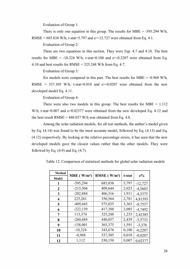
Evaluation of Group 1:
There is only one equation in this group. The results for MBE = -595.294 W/h,
RMSE = 685.838 W/h, t-stat=5.797 and e=-12.727 were obtained from Eq. 4.1.
Evaluation of Group 2:
There are two equations in this section. They were Eqs. 4.7 and 4.10. The best
results for MBE = -10.324 W/h, t-stat=0.100 and e=-0.2207 were obtained from Eq.
4.10 and best results for RMSE = 325.248 W/h from Eq. 4.7.
Evaluation of Group 3:
Six models were compared in this part. The best results for MBE = -0.968 W/h,
RMSE = 337.305 W/h, t-stat=0.010 and e=-0.0207 were obtained from the new
developed model Eq. 4.11.
Evaluation of Group 4:
There were also two models in this group. The best results for MBE = 1.112
W/h, t-stat=0.007 and e=0.02377 were obtained from the new developed Eq. 4.12 and
the best result RMSE = 440.037 W/h was obtained from Eq. 4.8.
Among the solar radiation models, for all test methods, the author’s model given
by Eq. (4.14) was found to be the most accurate model, followed by Eq. (4.13) and Eq.
(4.12) respectively. By looking at the relative percentage errors, it has seen that the new
developed models gave the closest values rather than the other models. They were
followed by Eq. (4.9) and Eq. (4.7).
Table 12. Comparison of statistical methods for global solar radiation models
Method
MBE ( W/m²) RMSE ( W/m²) t-stat e% Model
1 -595,294 685,838 5,797 -12,727 2 -213,304 409,644 2,023 -4,5603 3 -202,884 406,316 1,911 -4,3375 4 225,261 350,564 2,781 4,81593 5 -409,445 575,035 3,363 -8,7537 6 -222,139 417,388 2,085 -4,7492 7 113,374 325,248 1,233 2,42385 8 -260,684 440,037 2,439 -5,5733 9 -158,001 365,375 1,591 -3,378
10 -10,324 343,676 0,100 -0,2207 11 -0,968 337,305 0,010 -0,0207 12 1,112 530,150 0,007 0,02377
39
6.2. Results for Diffuse Solar Radiation
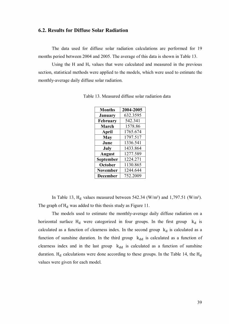
The data used for diffuse solar radiation calculations are performed for 19
months period between 2004 and 2005. The average of this data is shown in Table 13.
Using the H and Hₒ values that were calculated and measured in the previous
section, statistical methods were applied to the models, which were used to estimate the
monthly-average daily diffuse solar radiation.
Table 13. Measured diffuse solar radiation data
Months 2004-2005 January 632.3595 February 542.341
March 1578.86 April 1765.674 May 1797.517 June 1336.541 July 1433.864
August 1277.589 September 1224.271
October 1130.865 November 1244.644 December 752.2009
In Table 13, H values measured between 542.34 (W/m²) and 1,797.51 (W/m²).
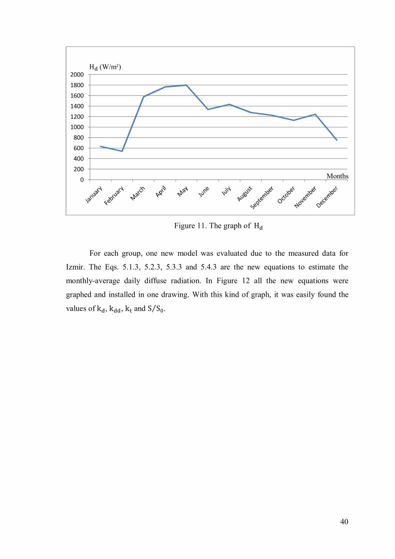
The graph of H was added to this thesis study as Figure 11.
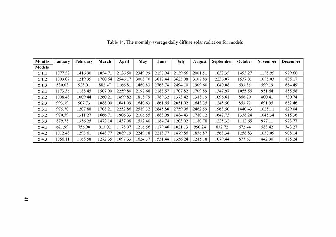
The models used to estimate the monthly-average daily diffuse radiation on a
horizontal surface H were categorized in four groups. In the first group k is
calculated as a function of clearness index. In the second group k is calculated as a
function of sunshine duration. In the third group k is calculated as a function of
clearness index and in the last group k is calculated as a function of sunshine
duration. H calculations were done according to these groups. In the Table 14, the H
values were given for each model.
40
Figure 11. The graph of H
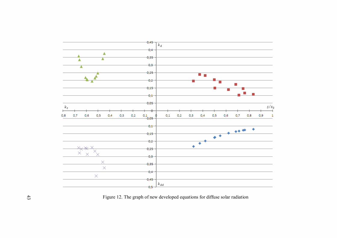
For each group, one new model was evaluated due to the measured data for
Izmir. The Eqs. 5.1.3, 5.2.3, 5.3.3 and 5.4.3 are the new equations to estimate the
monthly-average daily diffuse radiation. In Figure 12 all the new equations were
graphed and installed in one drawing. With this kind of graph, it was easily found the
values of k , k , k and S S⁄ .
0200400600800
100012001400160018002000
H (W/m²)
Months
41
Table 14. The monthly-average daily diffuse solar radiation for models
Months Models
January February March April May June July August September October November December
5.1.1 1077.52 1416.90 1854.71 2126.50 2349.99 2158.94 2139.66 2001.51 1832.35 1493.27 1155.95 979.66 5.1.2 1009.07 1219.95 1780.64 2546.17 3005.70 3812.44 3625.98 3107.89 2236.07 1537.81 1055.03 835.17 5.1.3 530.03 923.01 882.47 1166.81 1460.83 2763.78 2494.10 1909.60 1040.08 693.35 599.19 684.49 5.2.1 1173.36 1188.45 1507.90 2259.80 2197.68 2188.57 1707.82 1709.89 1347.97 1055.56 951.64 855.58 5.2.2 1008.48 1009.44 1260.21 1899.82 1818.79 1789.32 1373.42 1388.19 1096.61 866.20 800.41 730.74 5.2.3 993.39 907.73 1088.00 1641.09 1640.63 1861.65 2051.02 1643.35 1245.50 853.72 691.95 682.46 5.3.1 975.70 1207.88 1708.21 2252.86 2589.32 2845.80 2759.96 2462.59 1963.50 1440.43 1028.11 829.04 5.3.2 970.59 1311.27 1666.71 1906.33 2106.55 1888.99 1884.43 1780.12 1642.73 1338.24 1045.34 915.36 5.3.3 879.78 1356.25 1472.14 1437.08 1532.40 1184.74 1203.02 1180.78 1225.32 1112.65 977.11 973.77 5.4.1 621.99 756.90 913.02 1178.07 1216.56 1179.46 1021.13 990.24 832.72 672.44 583.42 543.27 5.4.2 1012.48 1293.61 1648.77 2089.19 2249.18 2213.77 1879.86 1856.87 1563.34 1258.83 1033.09 908.14 5.4.3 1056.11 1168.58 1272.35 1697.33 1624.37 1531.48 1356.24 1285.18 1079.44 877.63 842.90 875.24
42
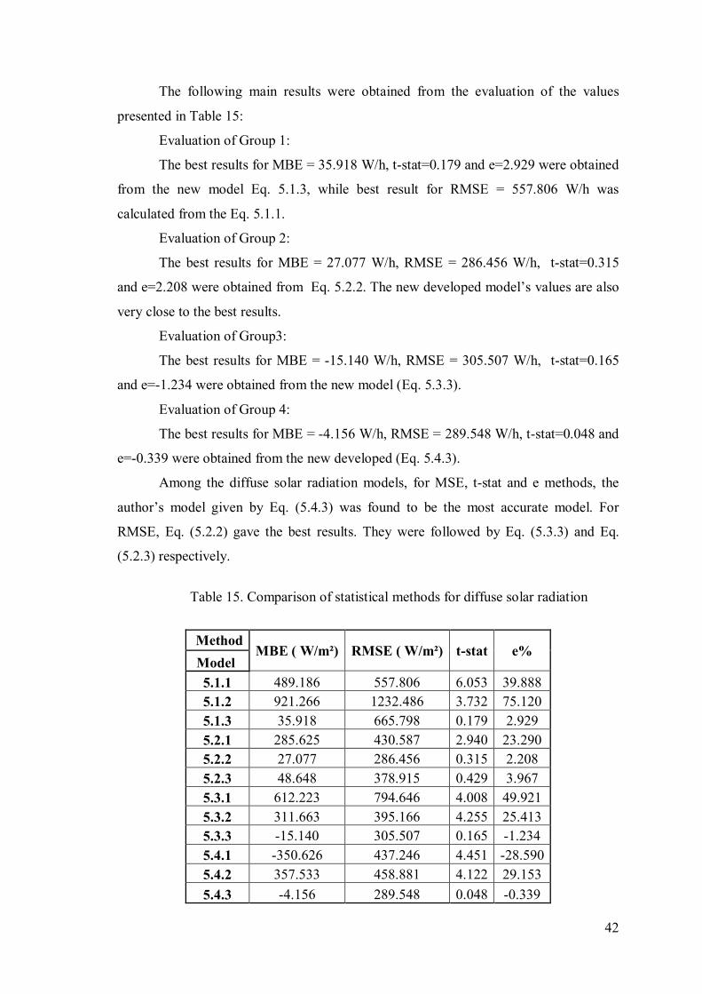
The following main results were obtained from the evaluation of the values
presented in Table 15:
Evaluation of Group 1:
The best results for MBE = 35.918 W/h, t-stat=0.179 and e=2.929 were obtained
from the new model Eq. 5.1.3, while best result for RMSE = 557.806 W/h was
calculated from the Eq. 5.1.1.
Evaluation of Group 2:
The best results for MBE = 27.077 W/h, RMSE = 286.456 W/h, t-stat=0.315
and e=2.208 were obtained from Eq. 5.2.2. The new developed model’s values are also
very close to the best results.
Evaluation of Group3:
The best results for MBE = -15.140 W/h, RMSE = 305.507 W/h, t-stat=0.165
and e=-1.234 were obtained from the new model (Eq. 5.3.3).
Evaluation of Group 4:
The best results for MBE = -4.156 W/h, RMSE = 289.548 W/h, t-stat=0.048 and
e=-0.339 were obtained from the new developed (Eq. 5.4.3).
Among the diffuse solar radiation models, for MSE, t-stat and e methods, the
author’s model given by Eq. (5.4.3) was found to be the most accurate model. For
RMSE, Eq. (5.2.2) gave the best results. They were followed by Eq. (5.3.3) and Eq.
(5.2.3) respectively.
Table 15. Comparison of statistical methods for diffuse solar radiation
Method
MBE ( W/m²) RMSE ( W/m²) t-stat e% Model 5.1.1 489.186 557.806 6.053 39.888 5.1.2 921.266 1232.486 3.732 75.120 5.1.3 35.918 665.798 0.179 2.929 5.2.1 285.625 430.587 2.940 23.290 5.2.2 27.077 286.456 0.315 2.208 5.2.3 48.648 378.915 0.429 3.967 5.3.1 612.223 794.646 4.008 49.921 5.3.2 311.663 395.166 4.255 25.413 5.3.3 -15.140 305.507 0.165 -1.234 5.4.1 -350.626 437.246 4.451 -28.590 5.4.2 357.533 458.881 4.122 29.153 5.4.3 -4.156 289.548 0.048 -0.339
43
Figure 12. The graph of new developed equations for diffuse solar radiation
44
CHAPTER 7
CONCLUSION
In this thesis, firstly solar radiation models for predicting the average daily and
hourly global and diffuse radiations on horizontal surface are reviewed. Then data of
global and diffuse solar radiations are analyzed from February, 2005 to May, 2007 and
from February, 2004 to December, 2005 on the campus area of IZTECH,
respectively. Empirical correlations are developed to estimate the monthly-average
daily global and diffuse radiations on a horizontal surface for Izmir, Turkey. 3 new
models are developed for estimating the monthly-average daily global solar radiation,
whereas 4 new models are developed for estimating the monthly-average daily diffuse
solar radiation. The developed models are compared with the models form the literature
on the basis of statistical methods namely, RMSE, MBE, T-stat and “e”. It is concluded that, the third-order polynomial equation gave the closest results
to the measured data for global solar radiation. The developed model given by Eq.
(4.14) is found to be the most accurate model for all test methods. For diffuse part, it is
concluded that the new models developed during this study are found to be reasonably
good for Izmir, Turkey comparing to the previous studies. The eq. (5.4.3) is found to
have the best results for MBE, t-stat and “e” methods. In RMSE the eq. (5.2.2) gave the
closest result according to the measured data. It can be deduced from the results that the new developed correlations are found
to be reasonably reliable for estimating or predicting the daily global and diffuse
radiations for Izmir, Turkey and, possibly, elsewhere with similar climatic condition.
45
LIST OF REFERENCES
Akinoglu, B. G. and Ecevit, A. (1990). Construction of a quadratic model using modified Angstrom coefficients to estimate global solar radiation. Solar Energy 45(2):85–92. Akpabio, L. E.; Udo S. O.; Etuk S. E. (2004), Empirical correlation of global solar radiation with Meteorological data for Onne, Nigeria. Turkish J.Physics, 28: 222-227. Aksoy, B. (1997), Estimated monthly average global radiation for Turkey and its comparison with observations, Renewable Energy, 10: 625-633 Angstrom, A. (1924), Solar and terrestrial radiation. Quart. Journal of the Royal Meteorological Society, 50:121–125. Aras, H.; Balli, O.; Hepbasli, A. (2006), Global Solar Potential. Part 1: Model Development, Energy Sources, Part B, 1(3):303-315 Barbaro S.; Cannato G.; Coppolina S.; Leone C; Sinagra E.( 1981), Diffuse solar radiation statistics for Italy. Solar Energy, 26:429–35 Che H. Z.; Shi G. Y.; Zhang X. Y.; Zhao J. Q.; Li Y. (2007), Analysis of sky condition using 40 years records of solar radiation data in china. Theoretical and applied climatology, 89: 83-94 Correspondence with Koray Ülgen. Diez-Mediavilla, M.; De Miguel, A.; Bilbao J (2005), Measurement and comparison of diffuse solar irradiance models on inclined surfaces in Valladolid (Spain).Energy Conversion and Management, 46: 2075-2092 El-Sebaii, A. A.; Al-Ghamdi, F. S.; Al-Hazmi and Adel S. Faidah (2009), Estimation of global solar radiation on horizontal surfaces in Jeddah, Saudi Arabia. Energy Policy, 37: 3654-3649 Gunes, M. (2001), Analysis of daily total horizontal solar radiation measurements in Turkey. Energy Sources 23:563–570.
46
Haydar A.; Balli O.; Hepbasli A. (2006), Estimating the horizontal diffuse solar radiation over the Central Anatolia region of Turkey. Energy Convers Manage, 47:2240–9 Haydar A.; Balli O.; Hepbasli A. (2006), Global solar radiation potential, Part 2: Statistical analysis. Energy Sources, 1:317–26 Inforse, (June,2011) http://www.inforse.dk/europe/dieret/Solar/solar.html Kaygusuz K.; Ayhan T. (1999), Analysis of solar radiation data for Trabzon, Turkey. Energy Convers Manage, 40:545–56 Kaygusuz, K. (1999),The comparison of measured and calculated solar radiations in Trabzon, Turkey. Energy Sources, 21:347–353 Kilic, A. ve Öztürk, A. (1983), Güneş Enerjisi, Kipaş Dağıtımcılık, İstanbul Kipp & Zonen, Pyranometer Instruction Manual (2000) Liu R. Y. H.; Jordan R. C. (1960), The interrelationship and characteristics distribution of direct, diffuse and total solar radiation. Solar Energy, 4(3):1–19 Ogelman, H.; Ecevit, A. and Tasdemiroglu, E. (1984), A new method for estimating solar radiation from bright sunshine data. Solar Energy, 33: 619-625 Ogulata, R. T. and Ogulata, S. N. (2002), Solar radiation on Adana, Turkey. Applied Energy, 71: 351–358 REN21 (2008). Global Status Report 2007 REN21 Secretariat, 51 pages. REN21 (2010). Renewables 2010 Global Status Report, p. 15-16. Sen, Z. and Tan, E. (2001), Simple models of solar radiation data for northwestern part of Turkey. Energy Convers Manage, 42:587–598.
47
Stone R. J. (1993) Improved statistical procedure for the evaluation of solar radiation estimation models. Solar Energy, 51(4):288–91 Tarhan, S.; Sari, A. (2005), Model selection for global and diffuse radiation over the Central Black Sea (CBS) region of Turkey. Energy Convers Manage, 46:605–13 Tasdemiroglu, E. and Sever, R. 1986. Monthly and yearly average maps of total and direct solar radiation in Turkey. Solar Energy 37:205–213. Tasdemiroglu E.; Sever, R. (1991), Estimation of monthly average daily, horizontal diffuse radiation in Turkey. Energy, 16(4):787–90 Tiris, M.; Tiris, C. and Ture, I. E. (1996), Correlations of monthly-average daily global, diffuse and beam radiations with hours of bright sunshine in Gebze, Turkey. Energy Convers Manage, 37(9): 1417–1421 Togrul, I. T. and E. Onat (1999), A study for estimating solar radiation in Elazig using geographical and meteorological data. Energy Convers Manage, 40: 1577–1584 Togrul, İ. T. and Togrul, H. (2002), Global solar radiation over Turkey: Comparison of predicted and measured data, Renewable Energy, 25: 55-67 Turkish Electrical Works Research Directorate http://www.eie.gov.tr/turkce/YEK/gunes/tgunes.html
Ulgen, K. and Hepbasli, A. (2004), Solar radiation models. Part 2: Comparison and developing new models, Energy Sources, 26: 521-530 Ulgen, K. ve Ozbalta, N., Measurement and evaluation of total solar radiation on horizantol surfaces in Bornova, Izmir, 12. Ulusal Isı Bilimi ve Tekniği Kongresi Ulgen, K. and Hepbasli, A. (2002), Comparison of solar radiation correlations for Izmir, Turkey. International Journal of Energy Research, 26: 413–430 Ulgen, K. and Hepbasli, A. (2002), Solar Radiation Models. Part 1: A Review. Energy Sources, 26: 413-430
48
Yildiz, M. and Oz, S. (1994), Evaluation of the solar energy potential of Turkey. In Proc. of the 6th National Energy Congress. Izmir, p. 250–260 (in Turkish). Yingni Jiang (2009) Estimation of monthly mean daily diffuse radiation in China. Applied Energy, 86:1458–1464
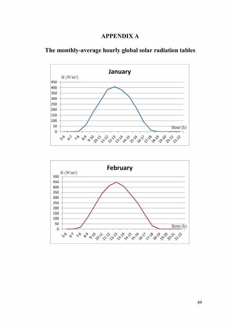
49
APPENDIX A
The monthly-average hourly global solar radiation tables
050
100150200250300350400450
January
050
100150200250300350400450500
February
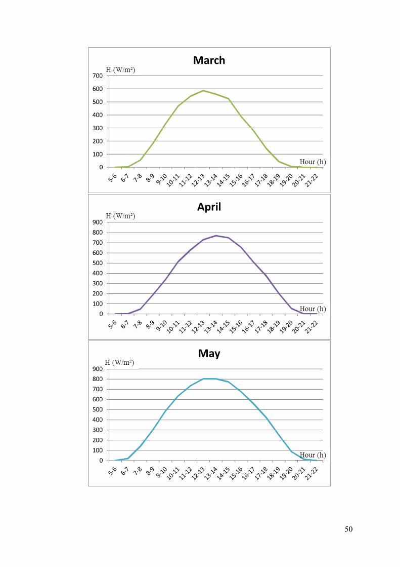
50
0
100
200
300
400
500
600
700
March
0100200300400500600700800900
April
0100200300400500600700800900
May
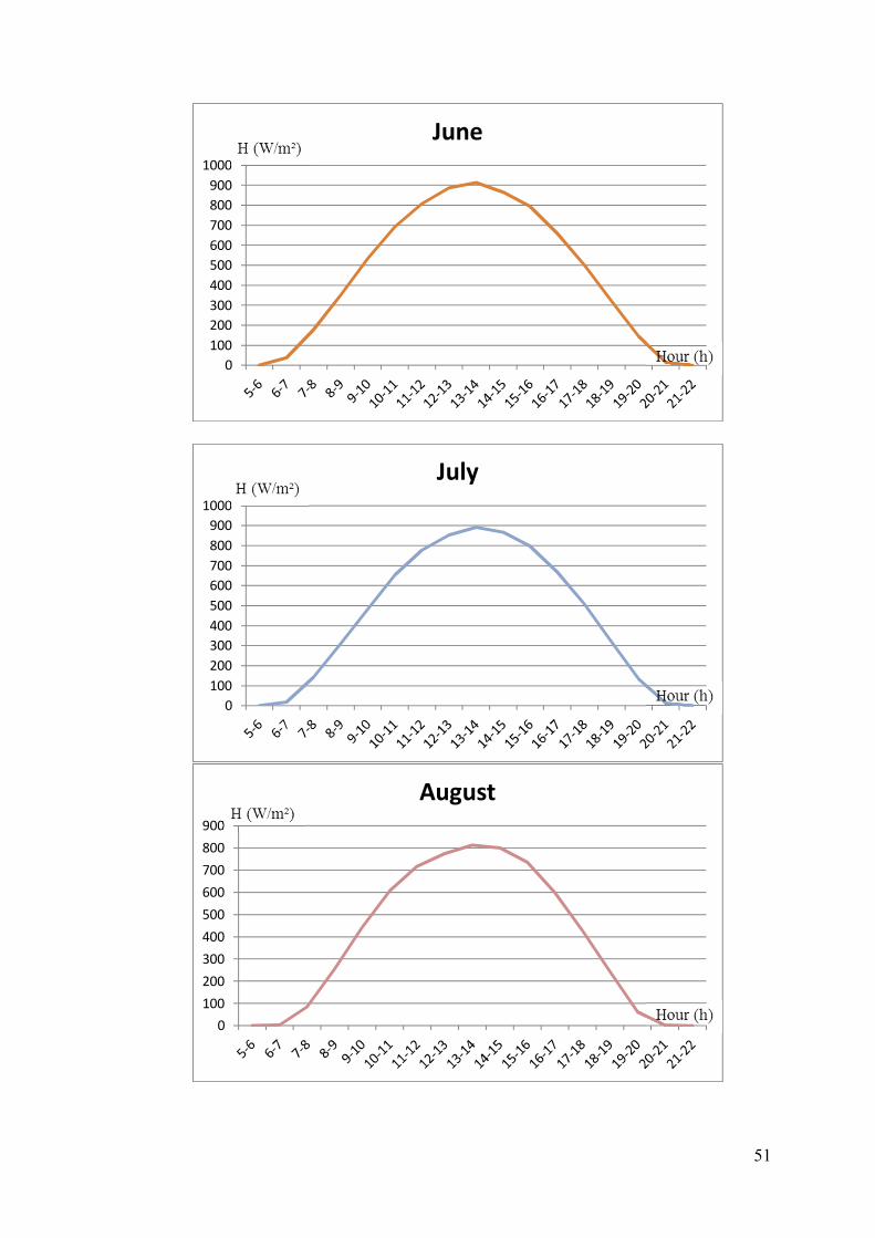
51
0100200300400500600700800900
1000
June
0100200300400500600700800900
1000
July
0100200300400500600700800900
August
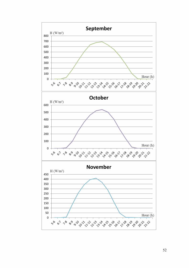
52
0
100
200
300
400
500
600
700
800
September
0
100
200
300
400
500
600
October
050
100150200250300350400450
November
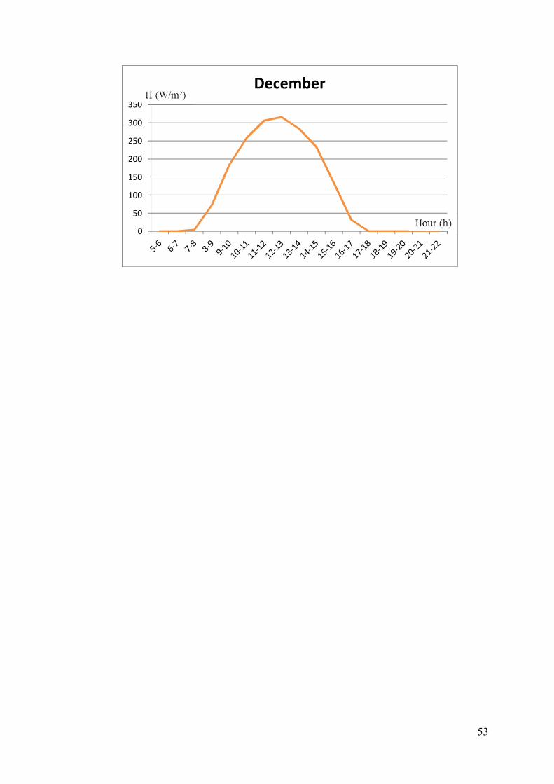
53
0
50
100
150
200
250
300
350
December