mcmc and gibbs sampling · approaches to inference lexact inference algorithms l the elimination...
TRANSCRIPT

MCMC and Gibbs Sampling
Kayhan Batmanghelich
1
Approaches to inferencel Exact inference algorithms
l The elimination algorithml Message-passing algorithm (sum-product, belief propagation)l The junction tree algorithms
l Approximate inference techniquesl Variational algorithms
l Loopy belief propagation l Mean field approximation
l Stochastic simulation / sampling methodsl Markov chain Monte Carlo methods
© Eric Xing @ CMU, 2005-2015 2
3
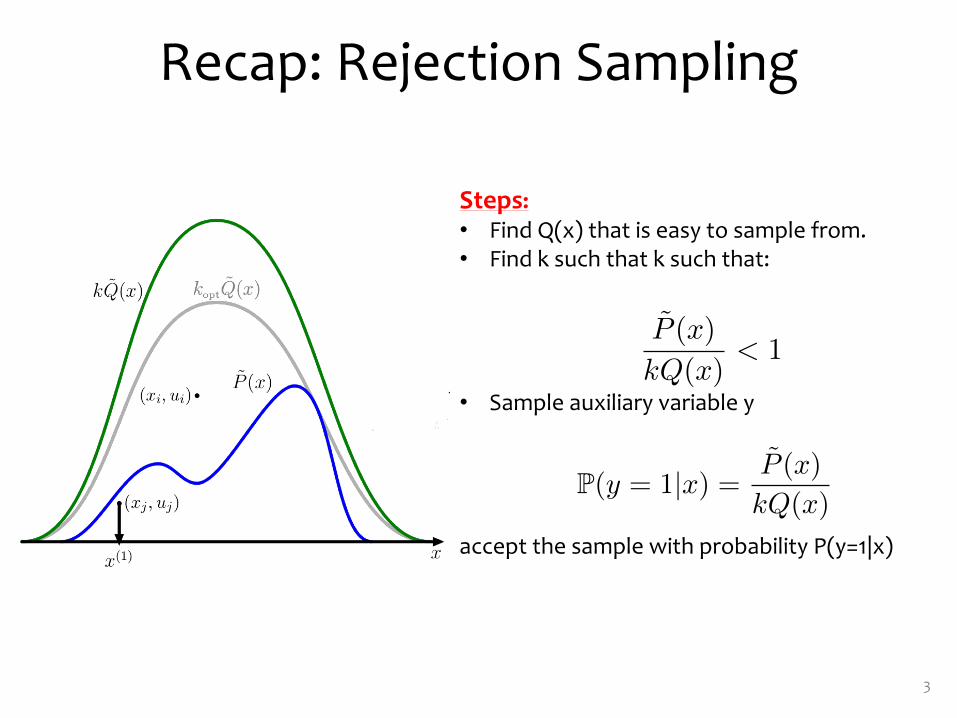
Recap: Rejection Sampling
Steps:• Find Q(x) that is easy to sample from.• Find k such that k such that:
• Sample auxiliary variable y
accept the sample with probability P(y=1|x)
P̃ (x)
kQ(x)< 1
<latexit sha1_base64="C3Pt6Y845+h/bz9d9nFnvLv4uK8=">AAACBnicbVDLSsNAFJ34rPUVdSnIYBHqpiQiqOCi6MZlC8YWmlAmk0k7dDIJMxOxhOzc+CtuXKi49Rvc+TdO2iy09cDlHs65l5l7/IRRqSzr21hYXFpeWa2sVdc3Nre2zZ3dOxmnAhMHxywWXR9JwignjqKKkW4iCIp8Rjr+6LrwO/dESBrzWzVOiBehAachxUhpqW8euKFAOHMVZQHJWnn94TjPRu2iwUto982a1bAmgPPELkkNlGj1zS83iHEaEa4wQ1L2bCtRXoaEopiRvOqmkiQIj9CA9DTlKCLSyyZ35PBIKwEMY6GLKzhRf29kKJJyHPl6MkJqKGe9QvzP66UqPPcyypNUEY6nD4UpgyqGRSgwoIJgxcaaICyo/ivEQ6SDUTq6qg7Bnj15njgnjYuG3T6tNa/KNCpgHxyCOrDBGWiCG9ACDsDgETyDV/BmPBkvxrvxMR1dMMqdPfAHxucP+TmYRA==</latexit><latexit sha1_base64="C3Pt6Y845+h/bz9d9nFnvLv4uK8=">AAACBnicbVDLSsNAFJ34rPUVdSnIYBHqpiQiqOCi6MZlC8YWmlAmk0k7dDIJMxOxhOzc+CtuXKi49Rvc+TdO2iy09cDlHs65l5l7/IRRqSzr21hYXFpeWa2sVdc3Nre2zZ3dOxmnAhMHxywWXR9JwignjqKKkW4iCIp8Rjr+6LrwO/dESBrzWzVOiBehAachxUhpqW8euKFAOHMVZQHJWnn94TjPRu2iwUto982a1bAmgPPELkkNlGj1zS83iHEaEa4wQ1L2bCtRXoaEopiRvOqmkiQIj9CA9DTlKCLSyyZ35PBIKwEMY6GLKzhRf29kKJJyHPl6MkJqKGe9QvzP66UqPPcyypNUEY6nD4UpgyqGRSgwoIJgxcaaICyo/ivEQ6SDUTq6qg7Bnj15njgnjYuG3T6tNa/KNCpgHxyCOrDBGWiCG9ACDsDgETyDV/BmPBkvxrvxMR1dMMqdPfAHxucP+TmYRA==</latexit><latexit sha1_base64="C3Pt6Y845+h/bz9d9nFnvLv4uK8=">AAACBnicbVDLSsNAFJ34rPUVdSnIYBHqpiQiqOCi6MZlC8YWmlAmk0k7dDIJMxOxhOzc+CtuXKi49Rvc+TdO2iy09cDlHs65l5l7/IRRqSzr21hYXFpeWa2sVdc3Nre2zZ3dOxmnAhMHxywWXR9JwignjqKKkW4iCIp8Rjr+6LrwO/dESBrzWzVOiBehAachxUhpqW8euKFAOHMVZQHJWnn94TjPRu2iwUto982a1bAmgPPELkkNlGj1zS83iHEaEa4wQ1L2bCtRXoaEopiRvOqmkiQIj9CA9DTlKCLSyyZ35PBIKwEMY6GLKzhRf29kKJJyHPl6MkJqKGe9QvzP66UqPPcyypNUEY6nD4UpgyqGRSgwoIJgxcaaICyo/ivEQ6SDUTq6qg7Bnj15njgnjYuG3T6tNa/KNCpgHxyCOrDBGWiCG9ACDsDgETyDV/BmPBkvxrvxMR1dMMqdPfAHxucP+TmYRA==</latexit><latexit sha1_base64="C3Pt6Y845+h/bz9d9nFnvLv4uK8=">AAACBnicbVDLSsNAFJ34rPUVdSnIYBHqpiQiqOCi6MZlC8YWmlAmk0k7dDIJMxOxhOzc+CtuXKi49Rvc+TdO2iy09cDlHs65l5l7/IRRqSzr21hYXFpeWa2sVdc3Nre2zZ3dOxmnAhMHxywWXR9JwignjqKKkW4iCIp8Rjr+6LrwO/dESBrzWzVOiBehAachxUhpqW8euKFAOHMVZQHJWnn94TjPRu2iwUto982a1bAmgPPELkkNlGj1zS83iHEaEa4wQ1L2bCtRXoaEopiRvOqmkiQIj9CA9DTlKCLSyyZ35PBIKwEMY6GLKzhRf29kKJJyHPl6MkJqKGe9QvzP66UqPPcyypNUEY6nD4UpgyqGRSgwoIJgxcaaICyo/ivEQ6SDUTq6qg7Bnj15njgnjYuG3T6tNa/KNCpgHxyCOrDBGWiCG9ACDsDgETyDV/BmPBkvxrvxMR1dMMqdPfAHxucP+TmYRA==</latexit>
P(y = 1|x) = P̃ (x)
kQ(x)<latexit sha1_base64="fc+7qCw5lWx1mpKmfwp1fwAzqCk=">AAACF3icbVA7T8MwGHR4lvIKMLJYVEjtUhKEBAyVKlgYW4nQSk1UOY7TWnUesh3UKPRnsPBXWBgAscLGv8FpM0DLSZZPd98n+86NGRXSML61peWV1bX10kZ5c2t7Z1ff278TUcIxsXDEIt51kSCMhsSSVDLSjTlBgctIxx1d537nnnBBo/BWpjFxAjQIqU8xkkrq6yd2gOTQdbPWpJo2zIdxDTag7XOEM1tS5pHcGNcm2aidX7CvV4y6MQVcJGZBKqBAq69/2V6Ek4CEEjMkRM80YulkiEuKGZmU7USQGOERGpCeoiEKiHCyabAJPFaKB/2IqxNKOFV/b2QoECINXDWZxxDzXi7+5/US6V84GQ3jRJIQzx7yEwZlBPOWoEc5wZKliiDMqforxEOkWpGqy7IqwZyPvEis0/pl3WyfVZpXRRslcAiOQBWY4Bw0wQ1oAQtg8AiewSt40560F+1d+5iNLmnFzgH4A+3zB6qHnxw=</latexit><latexit sha1_base64="fc+7qCw5lWx1mpKmfwp1fwAzqCk=">AAACF3icbVA7T8MwGHR4lvIKMLJYVEjtUhKEBAyVKlgYW4nQSk1UOY7TWnUesh3UKPRnsPBXWBgAscLGv8FpM0DLSZZPd98n+86NGRXSML61peWV1bX10kZ5c2t7Z1ff278TUcIxsXDEIt51kSCMhsSSVDLSjTlBgctIxx1d537nnnBBo/BWpjFxAjQIqU8xkkrq6yd2gOTQdbPWpJo2zIdxDTag7XOEM1tS5pHcGNcm2aidX7CvV4y6MQVcJGZBKqBAq69/2V6Ek4CEEjMkRM80YulkiEuKGZmU7USQGOERGpCeoiEKiHCyabAJPFaKB/2IqxNKOFV/b2QoECINXDWZxxDzXi7+5/US6V84GQ3jRJIQzx7yEwZlBPOWoEc5wZKliiDMqforxEOkWpGqy7IqwZyPvEis0/pl3WyfVZpXRRslcAiOQBWY4Bw0wQ1oAQtg8AiewSt40560F+1d+5iNLmnFzgH4A+3zB6qHnxw=</latexit><latexit sha1_base64="fc+7qCw5lWx1mpKmfwp1fwAzqCk=">AAACF3icbVA7T8MwGHR4lvIKMLJYVEjtUhKEBAyVKlgYW4nQSk1UOY7TWnUesh3UKPRnsPBXWBgAscLGv8FpM0DLSZZPd98n+86NGRXSML61peWV1bX10kZ5c2t7Z1ff278TUcIxsXDEIt51kSCMhsSSVDLSjTlBgctIxx1d537nnnBBo/BWpjFxAjQIqU8xkkrq6yd2gOTQdbPWpJo2zIdxDTag7XOEM1tS5pHcGNcm2aidX7CvV4y6MQVcJGZBKqBAq69/2V6Ek4CEEjMkRM80YulkiEuKGZmU7USQGOERGpCeoiEKiHCyabAJPFaKB/2IqxNKOFV/b2QoECINXDWZxxDzXi7+5/US6V84GQ3jRJIQzx7yEwZlBPOWoEc5wZKliiDMqforxEOkWpGqy7IqwZyPvEis0/pl3WyfVZpXRRslcAiOQBWY4Bw0wQ1oAQtg8AiewSt40560F+1d+5iNLmnFzgH4A+3zB6qHnxw=</latexit><latexit sha1_base64="fc+7qCw5lWx1mpKmfwp1fwAzqCk=">AAACF3icbVA7T8MwGHR4lvIKMLJYVEjtUhKEBAyVKlgYW4nQSk1UOY7TWnUesh3UKPRnsPBXWBgAscLGv8FpM0DLSZZPd98n+86NGRXSML61peWV1bX10kZ5c2t7Z1ff278TUcIxsXDEIt51kSCMhsSSVDLSjTlBgctIxx1d537nnnBBo/BWpjFxAjQIqU8xkkrq6yd2gOTQdbPWpJo2zIdxDTag7XOEM1tS5pHcGNcm2aidX7CvV4y6MQVcJGZBKqBAq69/2V6Ek4CEEjMkRM80YulkiEuKGZmU7USQGOERGpCeoiEKiHCyabAJPFaKB/2IqxNKOFV/b2QoECINXDWZxxDzXi7+5/US6V84GQ3jRJIQzx7yEwZlBPOWoEc5wZKliiDMqforxEOkWpGqy7IqwZyPvEis0/pl3WyfVZpXRRslcAiOQBWY4Bw0wQ1oAQtg8AiewSt40560F+1d+5iNLmnFzgH4A+3zB6qHnxw=</latexit>
4
Recap: Importance Sampling Importance sampling (2)
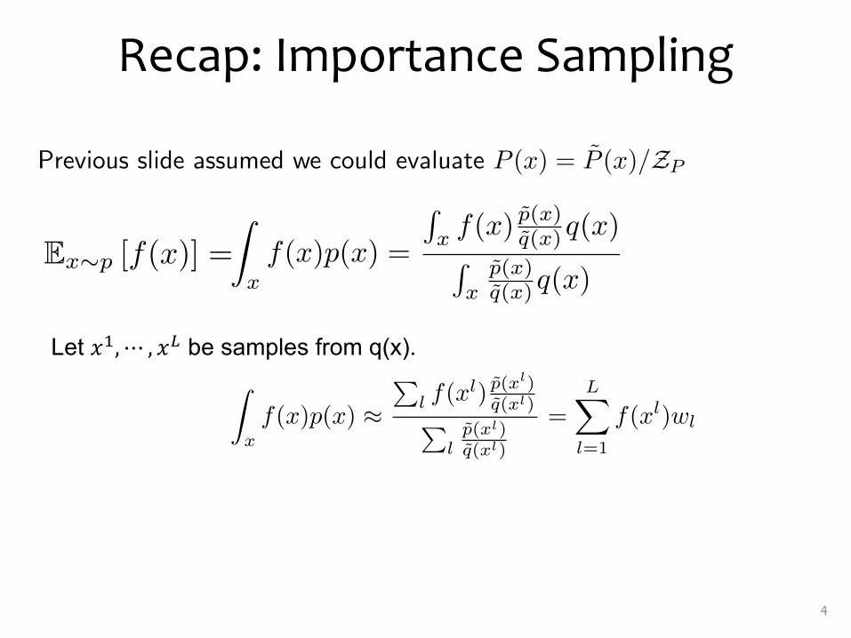
Previous slide assumed we could evaluate P (x) = P̃ (x)/ZP
!f(x)P (x) dx ≈ ZQ
ZP
1
S
S"
s=1
f(x(s))P̃ (x(s))
Q̃(x(s))# $% &r̃(s)
, x(s) ∼ Q(x)
≈✄✄✄✄✄✄1
S
S"
s=1
f(x(s))r̃(s)
✁✁✁✁1
S
's′ r̃
(s′)≡
S"
s=1
f(x(s))w(s)
This estimator is consistent but biased
Exercise: Prove that ZP/ZQ ≈ 1S
's r̃(s)
Let !",⋯ , !% be samples from q(x).
Z
xf(x)p(x) =
Rx f(x)
p̃(x)q̃(x)q(x)R
xp̃(x)q̃(x)q(x)
<latexit sha1_base64="9aLjmpz0Psa/aqaHEXhVmW1D3kE=">AAAC0niclVLPb9MwFHYyYKP8KnDk8kRVqbuUZELadpg0wYUDh1YibFpTRY7rbFYdx7OdqZWxBuLKX8eNf4G/AqcNUrdx4UmRP3/f+/Ls95xLzrSJol9BuHXv/oPtnYedR4+fPH3Wff7is65qRWhCKl6p0xxrypmgiWGG01OpKC5zTk/y+ftGP7miSrNKfDJLSaclPhesYAQbT2Xd3/20xOYiz+3IDZZH8ZfFLhxBWihMbGoYn9FGWOw6Ox83C3T6Z5mEN3CWjSHFUqpq0abHzn50kOq6zHhLOes6KRMmW0Dh3SAHG7+HTeVGRdlUBOcz1vvL1R4cXP7l187/cYHLur1oGK0C7oK4BT3Uxijr/kxnFalLKgzhWOtJHEkztVgZRjj1N6s1lZjM8TmdeChwSfXUrmbioO+ZGRSV8p8wsGI3HRaXWi/L3Gc2A9C3tYb8lzapTXEwtUzI2lBB1oWKmoOpoBkwzJiixPClB5go5s8K5AL7Phn/DDq+CfHtK98Fyd7wcBiP3/aO37Xd2EGv0Gs0QDHaR8foAxqhBJFgFFwF18HXMAlt+C38vk4Ng9bzEt2I8Mcfl1zdig==</latexit><latexit sha1_base64="9aLjmpz0Psa/aqaHEXhVmW1D3kE=">AAAC0niclVLPb9MwFHYyYKP8KnDk8kRVqbuUZELadpg0wYUDh1YibFpTRY7rbFYdx7OdqZWxBuLKX8eNf4G/AqcNUrdx4UmRP3/f+/Ls95xLzrSJol9BuHXv/oPtnYedR4+fPH3Wff7is65qRWhCKl6p0xxrypmgiWGG01OpKC5zTk/y+ftGP7miSrNKfDJLSaclPhesYAQbT2Xd3/20xOYiz+3IDZZH8ZfFLhxBWihMbGoYn9FGWOw6Ox83C3T6Z5mEN3CWjSHFUqpq0abHzn50kOq6zHhLOes6KRMmW0Dh3SAHG7+HTeVGRdlUBOcz1vvL1R4cXP7l187/cYHLur1oGK0C7oK4BT3Uxijr/kxnFalLKgzhWOtJHEkztVgZRjj1N6s1lZjM8TmdeChwSfXUrmbioO+ZGRSV8p8wsGI3HRaXWi/L3Gc2A9C3tYb8lzapTXEwtUzI2lBB1oWKmoOpoBkwzJiixPClB5go5s8K5AL7Phn/DDq+CfHtK98Fyd7wcBiP3/aO37Xd2EGv0Gs0QDHaR8foAxqhBJFgFFwF18HXMAlt+C38vk4Ng9bzEt2I8Mcfl1zdig==</latexit><latexit sha1_base64="9aLjmpz0Psa/aqaHEXhVmW1D3kE=">AAAC0niclVLPb9MwFHYyYKP8KnDk8kRVqbuUZELadpg0wYUDh1YibFpTRY7rbFYdx7OdqZWxBuLKX8eNf4G/AqcNUrdx4UmRP3/f+/Ls95xLzrSJol9BuHXv/oPtnYedR4+fPH3Wff7is65qRWhCKl6p0xxrypmgiWGG01OpKC5zTk/y+ftGP7miSrNKfDJLSaclPhesYAQbT2Xd3/20xOYiz+3IDZZH8ZfFLhxBWihMbGoYn9FGWOw6Ox83C3T6Z5mEN3CWjSHFUqpq0abHzn50kOq6zHhLOes6KRMmW0Dh3SAHG7+HTeVGRdlUBOcz1vvL1R4cXP7l187/cYHLur1oGK0C7oK4BT3Uxijr/kxnFalLKgzhWOtJHEkztVgZRjj1N6s1lZjM8TmdeChwSfXUrmbioO+ZGRSV8p8wsGI3HRaXWi/L3Gc2A9C3tYb8lzapTXEwtUzI2lBB1oWKmoOpoBkwzJiixPClB5go5s8K5AL7Phn/DDq+CfHtK98Fyd7wcBiP3/aO37Xd2EGv0Gs0QDHaR8foAxqhBJFgFFwF18HXMAlt+C38vk4Ng9bzEt2I8Mcfl1zdig==</latexit><latexit sha1_base64="9aLjmpz0Psa/aqaHEXhVmW1D3kE=">AAAC0niclVLPb9MwFHYyYKP8KnDk8kRVqbuUZELadpg0wYUDh1YibFpTRY7rbFYdx7OdqZWxBuLKX8eNf4G/AqcNUrdx4UmRP3/f+/Ls95xLzrSJol9BuHXv/oPtnYedR4+fPH3Wff7is65qRWhCKl6p0xxrypmgiWGG01OpKC5zTk/y+ftGP7miSrNKfDJLSaclPhesYAQbT2Xd3/20xOYiz+3IDZZH8ZfFLhxBWihMbGoYn9FGWOw6Ox83C3T6Z5mEN3CWjSHFUqpq0abHzn50kOq6zHhLOes6KRMmW0Dh3SAHG7+HTeVGRdlUBOcz1vvL1R4cXP7l187/cYHLur1oGK0C7oK4BT3Uxijr/kxnFalLKgzhWOtJHEkztVgZRjj1N6s1lZjM8TmdeChwSfXUrmbioO+ZGRSV8p8wsGI3HRaXWi/L3Gc2A9C3tYb8lzapTXEwtUzI2lBB1oWKmoOpoBkwzJiixPClB5go5s8K5AL7Phn/DDq+CfHtK98Fyd7wcBiP3/aO37Xd2EGv0Gs0QDHaR8foAxqhBJFgFFwF18HXMAlt+C38vk4Ng9bzEt2I8Mcfl1zdig==</latexit>
Z
xf(x)p(x) ⇡
Pl f(x
l) p̃(xl)
q̃(xl)P
lp̃(xl)q̃(xl)
=LX
l=1
f(xl)wl
<latexit sha1_base64="BB77UXZkEMVNag7Tr19P+0k1RJ0=">AAADgHiclVJbb9MwFHYTYCNc1sEjL0eUSu0DXYKQBkiVJnjhYQ+tRNm0posc19msOokXO9Aq+Hfwv3jjzyCcS6V23cssWT7+vvOdm04oOJPKdf+2LPvBw0d7+4+dJ0+fPT9oH774LtM8I3RCUp5m5yGWlLOEThRTnJ6LjOI45PQsXHwp+bMfNJMsTb6plaCzGF8lLGIEKwMFh63fXT/G6joMi5HurYber2UfhuBHGSaFrxif05JY9nWxGJcPON2LQMARXARj8LEQWbps3D1dnGrwZR4HvIF0oZ2uzxIVLCEychC9jfiwyWylFGVK0Maj/t9Uf9Bws8Zr5X1UoJ2dSrYbWNdu+Et+R0UluB29REz8Cq2191GZO6x1BR96+vJ0nflnwIN2xx241YFdw2uMDmrOKGj/8ecpyWOaKMKxlFPPFWpW4EwxwqnpPZdUYLLAV3RqzATHVM6KaoM0dA0yhyjNzE0UVOimosCxlKs4NJ7ltsjbXAnexU1zFX2YFSwRuaIJqRNFOQeVQrmOMGcZJYqvjIFJxkytQK6xmaAyS+uYIXi3W941Ju8GHwfe+H3n5HMzjX30Cr1GPeShY3SCvqIRmiDS+me9sd5aA9u2+/aR7dWuVqvRvERbx/70H1KeFyw=</latexit><latexit sha1_base64="BB77UXZkEMVNag7Tr19P+0k1RJ0=">AAADgHiclVJbb9MwFHYTYCNc1sEjL0eUSu0DXYKQBkiVJnjhYQ+tRNm0posc19msOokXO9Aq+Hfwv3jjzyCcS6V23cssWT7+vvOdm04oOJPKdf+2LPvBw0d7+4+dJ0+fPT9oH774LtM8I3RCUp5m5yGWlLOEThRTnJ6LjOI45PQsXHwp+bMfNJMsTb6plaCzGF8lLGIEKwMFh63fXT/G6joMi5HurYber2UfhuBHGSaFrxif05JY9nWxGJcPON2LQMARXARj8LEQWbps3D1dnGrwZR4HvIF0oZ2uzxIVLCEychC9jfiwyWylFGVK0Maj/t9Uf9Bws8Zr5X1UoJ2dSrYbWNdu+Et+R0UluB29REz8Cq2191GZO6x1BR96+vJ0nflnwIN2xx241YFdw2uMDmrOKGj/8ecpyWOaKMKxlFPPFWpW4EwxwqnpPZdUYLLAV3RqzATHVM6KaoM0dA0yhyjNzE0UVOimosCxlKs4NJ7ltsjbXAnexU1zFX2YFSwRuaIJqRNFOQeVQrmOMGcZJYqvjIFJxkytQK6xmaAyS+uYIXi3W941Ju8GHwfe+H3n5HMzjX30Cr1GPeShY3SCvqIRmiDS+me9sd5aA9u2+/aR7dWuVqvRvERbx/70H1KeFyw=</latexit><latexit sha1_base64="BB77UXZkEMVNag7Tr19P+0k1RJ0=">AAADgHiclVJbb9MwFHYTYCNc1sEjL0eUSu0DXYKQBkiVJnjhYQ+tRNm0posc19msOokXO9Aq+Hfwv3jjzyCcS6V23cssWT7+vvOdm04oOJPKdf+2LPvBw0d7+4+dJ0+fPT9oH774LtM8I3RCUp5m5yGWlLOEThRTnJ6LjOI45PQsXHwp+bMfNJMsTb6plaCzGF8lLGIEKwMFh63fXT/G6joMi5HurYber2UfhuBHGSaFrxif05JY9nWxGJcPON2LQMARXARj8LEQWbps3D1dnGrwZR4HvIF0oZ2uzxIVLCEychC9jfiwyWylFGVK0Maj/t9Uf9Bws8Zr5X1UoJ2dSrYbWNdu+Et+R0UluB29REz8Cq2191GZO6x1BR96+vJ0nflnwIN2xx241YFdw2uMDmrOKGj/8ecpyWOaKMKxlFPPFWpW4EwxwqnpPZdUYLLAV3RqzATHVM6KaoM0dA0yhyjNzE0UVOimosCxlKs4NJ7ltsjbXAnexU1zFX2YFSwRuaIJqRNFOQeVQrmOMGcZJYqvjIFJxkytQK6xmaAyS+uYIXi3W941Ju8GHwfe+H3n5HMzjX30Cr1GPeShY3SCvqIRmiDS+me9sd5aA9u2+/aR7dWuVqvRvERbx/70H1KeFyw=</latexit><latexit sha1_base64="BB77UXZkEMVNag7Tr19P+0k1RJ0=">AAADgHiclVJbb9MwFHYTYCNc1sEjL0eUSu0DXYKQBkiVJnjhYQ+tRNm0posc19msOokXO9Aq+Hfwv3jjzyCcS6V23cssWT7+vvOdm04oOJPKdf+2LPvBw0d7+4+dJ0+fPT9oH774LtM8I3RCUp5m5yGWlLOEThRTnJ6LjOI45PQsXHwp+bMfNJMsTb6plaCzGF8lLGIEKwMFh63fXT/G6joMi5HurYber2UfhuBHGSaFrxif05JY9nWxGJcPON2LQMARXARj8LEQWbps3D1dnGrwZR4HvIF0oZ2uzxIVLCEychC9jfiwyWylFGVK0Maj/t9Uf9Bws8Zr5X1UoJ2dSrYbWNdu+Et+R0UluB29REz8Cq2191GZO6x1BR96+vJ0nflnwIN2xx241YFdw2uMDmrOKGj/8ecpyWOaKMKxlFPPFWpW4EwxwqnpPZdUYLLAV3RqzATHVM6KaoM0dA0yhyjNzE0UVOimosCxlKs4NJ7ltsjbXAnexU1zFX2YFSwRuaIJqRNFOQeVQrmOMGcZJYqvjIFJxkytQK6xmaAyS+uYIXi3W941Ju8GHwfe+H3n5HMzjX30Cr1GPeShY3SCvqIRmiDS+me9sd5aA9u2+/aR7dWuVqvRvERbx/70H1KeFyw=</latexit>
Ex⇠p [f(x)] =<latexit sha1_base64="8DaO0lGvwvmIg3tHZz77mQExMxM=">AAACE3icbVDLSsNAFJ3UV62vqks3g0WoCCURQV0IRRFcVjC20IQymU7aoZMHMzfSEvoRbvwVNy5U3Lpx5984abPQ1gMDh3Pu5c45Xiy4AtP8NgoLi0vLK8XV0tr6xuZWeXvnXkWJpMymkYhkyyOKCR4yGzgI1oolI4EnWNMbXGV+84FJxaPwDkYxcwPSC7nPKQEtdcpHTkCg73np9biTDrGjeIDjMXYE86GN/erwEDuS9/rg4otOuWLWzAnwPLFyUkE5Gp3yl9ONaBKwEKggSrUtMwY3JRI4FWxcchLFYkIHpMfamoYkYMpNJ6HG+EArXexHUr8Q8ET9vZGSQKlR4OnJLIKa9TLxP6+dgH/mpjyME2AhnR7yE4EhwllDuMsloyBGmhAquf4rpn0iCQXdY0mXYM1Gnif2ce28Zt2eVOqXeRtFtIf2URVZ6BTV0Q1qIBtR9Iie0St6M56MF+Pd+JiOFox8Zxf9gfH5A6e/nX0=</latexit><latexit sha1_base64="8DaO0lGvwvmIg3tHZz77mQExMxM=">AAACE3icbVDLSsNAFJ3UV62vqks3g0WoCCURQV0IRRFcVjC20IQymU7aoZMHMzfSEvoRbvwVNy5U3Lpx5984abPQ1gMDh3Pu5c45Xiy4AtP8NgoLi0vLK8XV0tr6xuZWeXvnXkWJpMymkYhkyyOKCR4yGzgI1oolI4EnWNMbXGV+84FJxaPwDkYxcwPSC7nPKQEtdcpHTkCg73np9biTDrGjeIDjMXYE86GN/erwEDuS9/rg4otOuWLWzAnwPLFyUkE5Gp3yl9ONaBKwEKggSrUtMwY3JRI4FWxcchLFYkIHpMfamoYkYMpNJ6HG+EArXexHUr8Q8ET9vZGSQKlR4OnJLIKa9TLxP6+dgH/mpjyME2AhnR7yE4EhwllDuMsloyBGmhAquf4rpn0iCQXdY0mXYM1Gnif2ce28Zt2eVOqXeRtFtIf2URVZ6BTV0Q1qIBtR9Iie0St6M56MF+Pd+JiOFox8Zxf9gfH5A6e/nX0=</latexit><latexit sha1_base64="8DaO0lGvwvmIg3tHZz77mQExMxM=">AAACE3icbVDLSsNAFJ3UV62vqks3g0WoCCURQV0IRRFcVjC20IQymU7aoZMHMzfSEvoRbvwVNy5U3Lpx5984abPQ1gMDh3Pu5c45Xiy4AtP8NgoLi0vLK8XV0tr6xuZWeXvnXkWJpMymkYhkyyOKCR4yGzgI1oolI4EnWNMbXGV+84FJxaPwDkYxcwPSC7nPKQEtdcpHTkCg73np9biTDrGjeIDjMXYE86GN/erwEDuS9/rg4otOuWLWzAnwPLFyUkE5Gp3yl9ONaBKwEKggSrUtMwY3JRI4FWxcchLFYkIHpMfamoYkYMpNJ6HG+EArXexHUr8Q8ET9vZGSQKlR4OnJLIKa9TLxP6+dgH/mpjyME2AhnR7yE4EhwllDuMsloyBGmhAquf4rpn0iCQXdY0mXYM1Gnif2ce28Zt2eVOqXeRtFtIf2URVZ6BTV0Q1qIBtR9Iie0St6M56MF+Pd+JiOFox8Zxf9gfH5A6e/nX0=</latexit><latexit sha1_base64="8DaO0lGvwvmIg3tHZz77mQExMxM=">AAACE3icbVDLSsNAFJ3UV62vqks3g0WoCCURQV0IRRFcVjC20IQymU7aoZMHMzfSEvoRbvwVNy5U3Lpx5984abPQ1gMDh3Pu5c45Xiy4AtP8NgoLi0vLK8XV0tr6xuZWeXvnXkWJpMymkYhkyyOKCR4yGzgI1oolI4EnWNMbXGV+84FJxaPwDkYxcwPSC7nPKQEtdcpHTkCg73np9biTDrGjeIDjMXYE86GN/erwEDuS9/rg4otOuWLWzAnwPLFyUkE5Gp3yl9ONaBKwEKggSrUtMwY3JRI4FWxcchLFYkIHpMfamoYkYMpNJ6HG+EArXexHUr8Q8ET9vZGSQKlR4OnJLIKa9TLxP6+dgH/mpjyME2AhnR7yE4EhwllDuMsloyBGmhAquf4rpn0iCQXdY0mXYM1Gnif2ce28Zt2eVOqXeRtFtIf2URVZ6BTV0Q1qIBtR9Iie0St6M56MF+Pd+JiOFox8Zxf9gfH5A6e/nX0=</latexit>
5
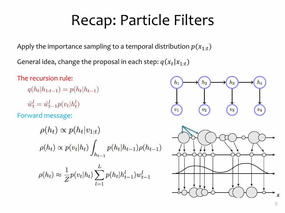
Recap: Particle FiltersApply the importance sampling to a temporal distribution !(#$:&)
General idea, change the proposal in each step: ( #& #$:&)
The recursion rule:
Forward message:
Summary so far
6
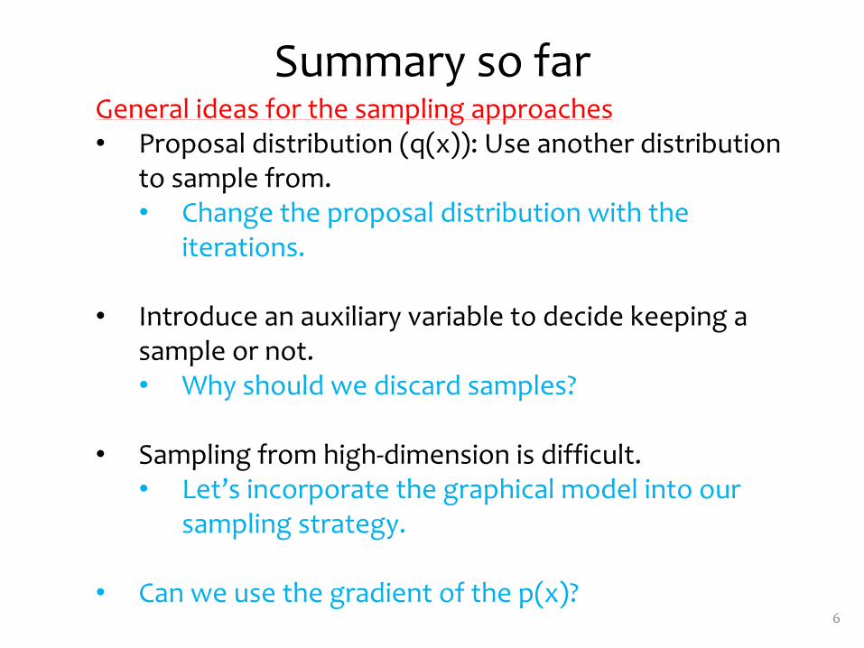
General ideas for the sampling approaches• Proposal distribution (q(x)): Use another distribution
to sample from.• Change the proposal distribution with the
iterations.
• Introduce an auxiliary variable to decide keeping a sample or not.• Why should we discard samples?
• Sampling from high-dimension is difficult.• Let’s incorporate the graphical model into our
sampling strategy.
• Can we use the gradient of the p(x)?
Summary so far
7
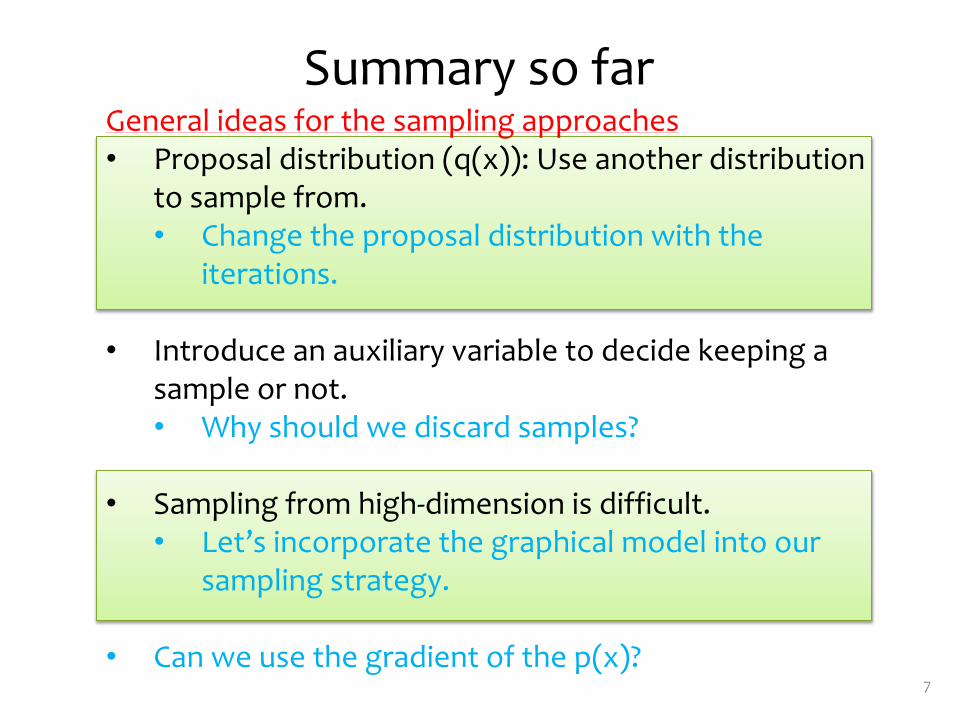
General ideas for the sampling approaches• Proposal distribution (q(x)): Use another distribution
to sample from.• Change the proposal distribution with the
iterations.
• Introduce an auxiliary variable to decide keeping a sample or not.• Why should we discard samples?
• Sampling from high-dimension is difficult.• Let’s incorporate the graphical model into our
sampling strategy.
• Can we use the gradient of the p(x)?
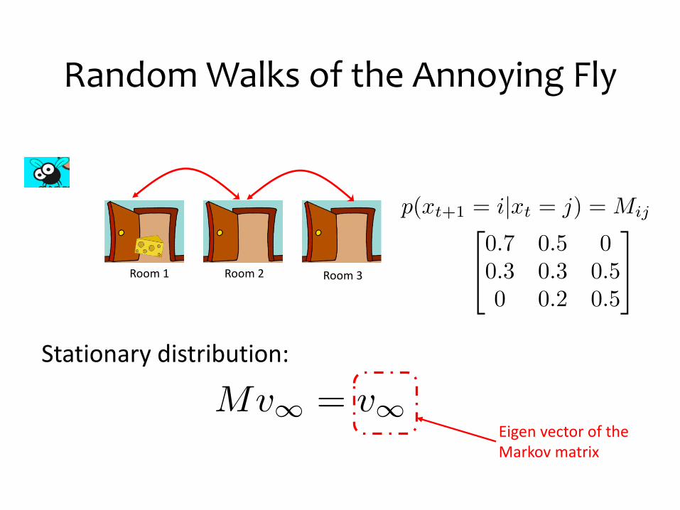
Random Walks of the Annoying Fly
Room 1 Room 2 Room 3
p(xt+1 = i|xt = j) = Mij2
40.7 0.5 00.3 0.3 0.50 0.2 0.5
3
5
Stationary distribution:
Mv1 = v1<latexit sha1_base64="WBXYijMaIEMeBe6QQKQHMXzFhPU=">AAACAHicbZDNSsNAFIVv6l+tf1E3gpvBIrgqiQjqQii6cSNUMLbQhjKZTtqhk0mYmRRKqBtfxY0LFbc+hjvfxmkbUFsPDHycey937gkSzpR2nC+rsLC4tLxSXC2trW9sbtnbO/cqTiWhHol5LBsBVpQzQT3NNKeNRFIcBZzWg/7VuF4fUKlYLO70MKF+hLuChYxgbay2vXeDBu2sxUSohyN08cNtu+xUnInQPLg5lCFXrW1/tjoxSSMqNOFYqabrJNrPsNSMcDoqtVJFE0z6uEubBgWOqPKzyQUjdGicDgpjaZ7QaOL+nshwpNQwCkxnhHVPzdbG5n+1ZqrDMz9jIkk1FWS6KEw50jEax4E6TFKi+dAAJpKZvyLSwxITbUIrmRDc2ZPnwTuunFfc25Ny9TJPowj7cABH4MIpVOEaauABgQd4ghd4tR6tZ+vNep+2Fqx8Zhf+yPr4Bhbolt8=</latexit><latexit sha1_base64="WBXYijMaIEMeBe6QQKQHMXzFhPU=">AAACAHicbZDNSsNAFIVv6l+tf1E3gpvBIrgqiQjqQii6cSNUMLbQhjKZTtqhk0mYmRRKqBtfxY0LFbc+hjvfxmkbUFsPDHycey937gkSzpR2nC+rsLC4tLxSXC2trW9sbtnbO/cqTiWhHol5LBsBVpQzQT3NNKeNRFIcBZzWg/7VuF4fUKlYLO70MKF+hLuChYxgbay2vXeDBu2sxUSohyN08cNtu+xUnInQPLg5lCFXrW1/tjoxSSMqNOFYqabrJNrPsNSMcDoqtVJFE0z6uEubBgWOqPKzyQUjdGicDgpjaZ7QaOL+nshwpNQwCkxnhHVPzdbG5n+1ZqrDMz9jIkk1FWS6KEw50jEax4E6TFKi+dAAJpKZvyLSwxITbUIrmRDc2ZPnwTuunFfc25Ny9TJPowj7cABH4MIpVOEaauABgQd4ghd4tR6tZ+vNep+2Fqx8Zhf+yPr4Bhbolt8=</latexit><latexit sha1_base64="WBXYijMaIEMeBe6QQKQHMXzFhPU=">AAACAHicbZDNSsNAFIVv6l+tf1E3gpvBIrgqiQjqQii6cSNUMLbQhjKZTtqhk0mYmRRKqBtfxY0LFbc+hjvfxmkbUFsPDHycey937gkSzpR2nC+rsLC4tLxSXC2trW9sbtnbO/cqTiWhHol5LBsBVpQzQT3NNKeNRFIcBZzWg/7VuF4fUKlYLO70MKF+hLuChYxgbay2vXeDBu2sxUSohyN08cNtu+xUnInQPLg5lCFXrW1/tjoxSSMqNOFYqabrJNrPsNSMcDoqtVJFE0z6uEubBgWOqPKzyQUjdGicDgpjaZ7QaOL+nshwpNQwCkxnhHVPzdbG5n+1ZqrDMz9jIkk1FWS6KEw50jEax4E6TFKi+dAAJpKZvyLSwxITbUIrmRDc2ZPnwTuunFfc25Ny9TJPowj7cABH4MIpVOEaauABgQd4ghd4tR6tZ+vNep+2Fqx8Zhf+yPr4Bhbolt8=</latexit><latexit sha1_base64="WBXYijMaIEMeBe6QQKQHMXzFhPU=">AAACAHicbZDNSsNAFIVv6l+tf1E3gpvBIrgqiQjqQii6cSNUMLbQhjKZTtqhk0mYmRRKqBtfxY0LFbc+hjvfxmkbUFsPDHycey937gkSzpR2nC+rsLC4tLxSXC2trW9sbtnbO/cqTiWhHol5LBsBVpQzQT3NNKeNRFIcBZzWg/7VuF4fUKlYLO70MKF+hLuChYxgbay2vXeDBu2sxUSohyN08cNtu+xUnInQPLg5lCFXrW1/tjoxSSMqNOFYqabrJNrPsNSMcDoqtVJFE0z6uEubBgWOqPKzyQUjdGicDgpjaZ7QaOL+nshwpNQwCkxnhHVPzdbG5n+1ZqrDMz9jIkk1FWS6KEw50jEax4E6TFKi+dAAJpKZvyLSwxITbUIrmRDc2ZPnwTuunFfc25Ny9TJPowj7cABH4MIpVOEaauABgQd4ghd4tR6tZ+vNep+2Fqx8Zhf+yPr4Bhbolt8=</latexit>
Eigen vector of the Markov matrix

GIBBS SAMPLINGExploiting the structure
9
Gibbs Sampling
10
Copyright Cambridge University Press 2003. On-screen viewing permitted. Printing not permitted. http://www.cambridge.org/0521642981You can buy this book for 30 pounds or $50. See http://www.inference.phy.cam.ac.uk/mackay/itila/ for links.
370 29 — Monte Carlo Methods
(a)x1
x2
P (x)
(b)x1
x2
P (x1 |x(t)2 )
x(t)
(c)x1
x2
P (x2 |x1)
(d)x1
x2
x(t)
x(t+1)
x(t+2)
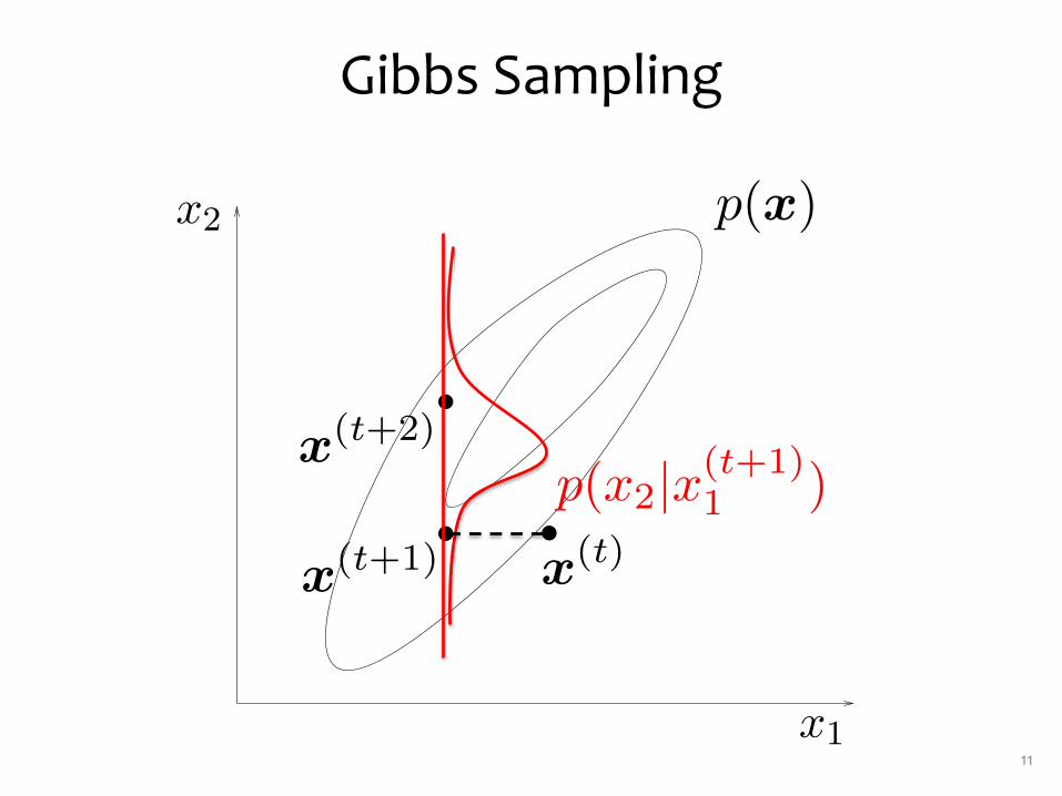
Figure 29.13. Gibbs sampling.(a) The joint density P (x) fromwhich samples are required. (b)Starting from a state x(t), x1 issampled from the conditionaldensity P (x1 |x(t)
2 ). (c) A sampleis then made from the conditionaldensity P (x2 |x1). (d) A couple ofiterations of Gibbs sampling.
This is good news and bad news. It is good news because, unlike thecases of rejection sampling and importance sampling, there is no catastrophicdependence on the dimensionality N . Our computer will give useful answersin a time shorter than the age of the universe. But it is bad news all the same,because this quadratic dependence on the lengthscale-ratio may still force usto make very lengthy simulations.
Fortunately, there are methods for suppressing random walks in MonteCarlo simulations, which we will discuss in the next chapter.
29.5 Gibbs sampling
We introduced importance sampling, rejection sampling and the Metropolismethod using one-dimensional examples. Gibbs sampling, also known as theheat bath method or ‘Glauber dynamics’, is a method for sampling from dis-tributions over at least two dimensions. Gibbs sampling can be viewed as aMetropolis method in which a sequence of proposal distributions Q are definedin terms of the conditional distributions of the joint distribution P (x). It isassumed that, whilst P (x) is too complex to draw samples from directly, itsconditional distributions P (xi | {xj}j ̸=i) are tractable to work with. For manygraphical models (but not all) these one-dimensional conditional distributionsare straightforward to sample from. For example, if a Gaussian distributionfor some variables d has an unknown mean m, and the prior distribution of mis Gaussian, then the conditional distribution of m given d is also Gaussian.Conditional distributions that are not of standard form may still be sampledfrom by adaptive rejection sampling if the conditional distribution satisfiescertain convexity properties (Gilks and Wild, 1992).
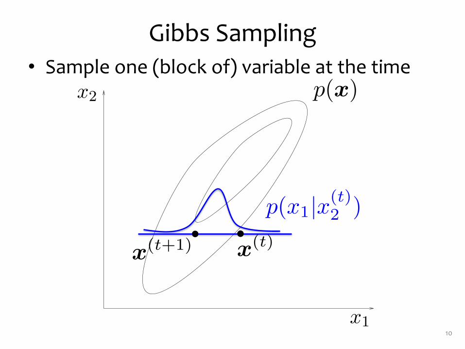
Gibbs sampling is illustrated for a case with two variables (x1, x2) = xin figure 29.13. On each iteration, we start from the current state x(t), andx1 is sampled from the conditional density P (x1 |x2), with x2 fixed to x(t)
2 .A sample x2 is then made from the conditional density P (x2 |x1), using the
p(x)
p(x1|x(t)2 )
x(t)x(t+1)
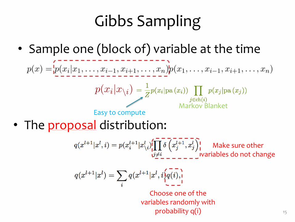
• Sample one (block of) variable at the time
Gibbs Sampling
11
Copyright Cambridge University Press 2003. On-screen viewing permitted. Printing not permitted. http://www.cambridge.org/0521642981You can buy this book for 30 pounds or $50. See http://www.inference.phy.cam.ac.uk/mackay/itila/ for links.
370 29 — Monte Carlo Methods
(a)x1
x2
P (x)
(b)x1
x2
P (x1 |x(t)2 )
x(t)
(c)x1
x2
P (x2 |x1)
(d)x1
x2
x(t)
x(t+1)
x(t+2)
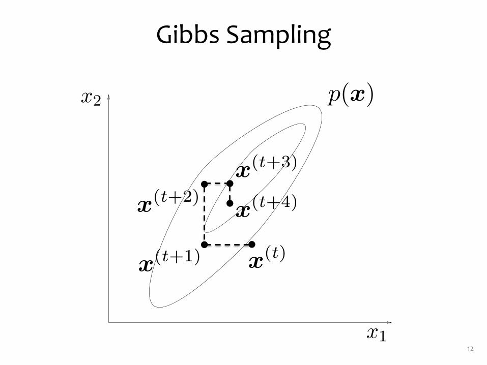
Figure 29.13. Gibbs sampling.(a) The joint density P (x) fromwhich samples are required. (b)Starting from a state x(t), x1 issampled from the conditionaldensity P (x1 |x(t)
2 ). (c) A sampleis then made from the conditionaldensity P (x2 |x1). (d) A couple ofiterations of Gibbs sampling.
This is good news and bad news. It is good news because, unlike thecases of rejection sampling and importance sampling, there is no catastrophicdependence on the dimensionality N . Our computer will give useful answersin a time shorter than the age of the universe. But it is bad news all the same,because this quadratic dependence on the lengthscale-ratio may still force usto make very lengthy simulations.
Fortunately, there are methods for suppressing random walks in MonteCarlo simulations, which we will discuss in the next chapter.
29.5 Gibbs sampling
We introduced importance sampling, rejection sampling and the Metropolismethod using one-dimensional examples. Gibbs sampling, also known as theheat bath method or ‘Glauber dynamics’, is a method for sampling from dis-tributions over at least two dimensions. Gibbs sampling can be viewed as aMetropolis method in which a sequence of proposal distributions Q are definedin terms of the conditional distributions of the joint distribution P (x). It isassumed that, whilst P (x) is too complex to draw samples from directly, itsconditional distributions P (xi | {xj}j ̸=i) are tractable to work with. For manygraphical models (but not all) these one-dimensional conditional distributionsare straightforward to sample from. For example, if a Gaussian distributionfor some variables d has an unknown mean m, and the prior distribution of mis Gaussian, then the conditional distribution of m given d is also Gaussian.Conditional distributions that are not of standard form may still be sampledfrom by adaptive rejection sampling if the conditional distribution satisfiescertain convexity properties (Gilks and Wild, 1992).
Gibbs sampling is illustrated for a case with two variables (x1, x2) = xin figure 29.13. On each iteration, we start from the current state x(t), andx1 is sampled from the conditional density P (x1 |x2), with x2 fixed to x(t)
2 .A sample x2 is then made from the conditional density P (x2 |x1), using the
p(x)
x(t+1)
x(t+2)
p(x2|x(t+1)1 )
x(t)
Gibbs Sampling
12
Copyright Cambridge University Press 2003. On-screen viewing permitted. Printing not permitted. http://www.cambridge.org/0521642981You can buy this book for 30 pounds or $50. See http://www.inference.phy.cam.ac.uk/mackay/itila/ for links.
370 29 — Monte Carlo Methods
(a)x1
x2
P (x)
(b)x1
x2
P (x1 |x(t)2 )
x(t)
(c)x1
x2
P (x2 |x1)
(d)x1
x2
x(t)
x(t+1)
x(t+2)
Figure 29.13. Gibbs sampling.(a) The joint density P (x) fromwhich samples are required. (b)Starting from a state x(t), x1 issampled from the conditionaldensity P (x1 |x(t)
2 ). (c) A sampleis then made from the conditionaldensity P (x2 |x1). (d) A couple ofiterations of Gibbs sampling.
This is good news and bad news. It is good news because, unlike thecases of rejection sampling and importance sampling, there is no catastrophicdependence on the dimensionality N . Our computer will give useful answersin a time shorter than the age of the universe. But it is bad news all the same,because this quadratic dependence on the lengthscale-ratio may still force usto make very lengthy simulations.
Fortunately, there are methods for suppressing random walks in MonteCarlo simulations, which we will discuss in the next chapter.
29.5 Gibbs sampling
We introduced importance sampling, rejection sampling and the Metropolismethod using one-dimensional examples. Gibbs sampling, also known as theheat bath method or ‘Glauber dynamics’, is a method for sampling from dis-tributions over at least two dimensions. Gibbs sampling can be viewed as aMetropolis method in which a sequence of proposal distributions Q are definedin terms of the conditional distributions of the joint distribution P (x). It isassumed that, whilst P (x) is too complex to draw samples from directly, itsconditional distributions P (xi | {xj}j ̸=i) are tractable to work with. For manygraphical models (but not all) these one-dimensional conditional distributionsare straightforward to sample from. For example, if a Gaussian distributionfor some variables d has an unknown mean m, and the prior distribution of mis Gaussian, then the conditional distribution of m given d is also Gaussian.Conditional distributions that are not of standard form may still be sampledfrom by adaptive rejection sampling if the conditional distribution satisfiescertain convexity properties (Gilks and Wild, 1992).
Gibbs sampling is illustrated for a case with two variables (x1, x2) = xin figure 29.13. On each iteration, we start from the current state x(t), andx1 is sampled from the conditional density P (x1 |x2), with x2 fixed to x(t)
2 .A sample x2 is then made from the conditional density P (x2 |x1), using the
p(x)
x(t+1)
x(t+2)
x(t)
x(t+3)
x(t+4)
Gibbs Sampling
13
Link:https://www.youtube.com/watch?v=AEwY6QXWoUghttps://www.youtube.com/watch?v=ZaKwpVgmKTY
Ingredients for Gibb Recipe
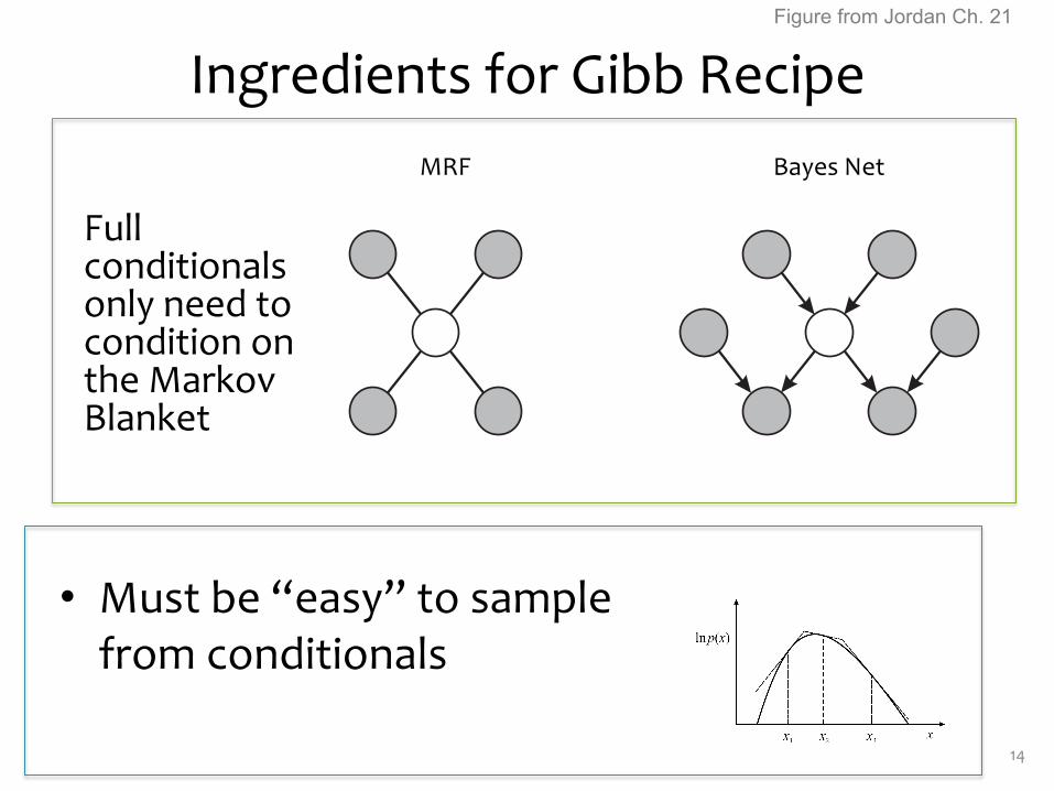
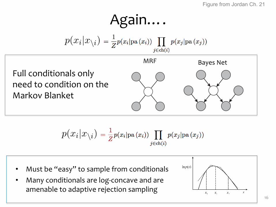
Full conditionals only need to condition on the Markov Blanket
14
1.3. GIBBS SAMPLING 25
drawn from conditional distributions . In the case of graphical models, the conditionaldistributions for individual nodes depend only on the variables in the corresponding Markov blan-kets, as illustrated in Figure ??. For directed graphs, a very broad choice of conditional distribu-
(a) (b)
Figure 1.15: The Gibbs sampling requires samples to be drawn from the conditional distribution ofa variable conditioned on the remaining variables. For graphical models, this conditional distribu-tion is a function only of the states of the nodes in the Markov blanket. In the case of an undirectedgraph (a) this comprises the set of neighbours while for a directed graph (b) the Markov blanketcomprises the parents, the children and the co-parents.
tions for the individual nodes conditioned on their parents will lead to conditional distributionsfor Gibbs sampling which are log concave. The adaptive rejection sampling methods discussedin Section ?? therefore provide a framework for Monte Carlo sampling from directed graphs withbroad applicability.
As with the Metropolis algorithm, we can gain some insight into the behaviour of Gibbs sam-pling by investigating its application to a Gaussian distribution. Consider a correlated Gaussian intwo variables, as illustrated in Figure ??, having a conditional distribution of width and a marginaldistribution of width . The typical step size is governed by the conditional distributions and willbe of order . Since the state evolves according to a random walk, the number of steps needed to ob-tain independent samples from the distribution will be of order . Of course if the Gaussiandistribution were uncorrelated then the Gibbs sampling procedure would be optimally efficient.For this simple problem we could rotate the coordinate system in order to decorrelate the variable,however, in practical applications it will generally be infeasible to find such transformations.
One approach to reducing random walk behaviour in Gibbs sampling is called over-relaxation.In its original form this applies to problems for which the conditional distributions are Gaussian.This represents a more general class of distributions than the multi-variate Gaussian, since for ex-ample the non-Gaussian distribution has Gaussian conditional distributions.At each step of the Gibbs sampling algorithm the conditional distribution for a particular compo-nent has some mean and some variance . In the over-relaxation framework the value ofis replaced with
(1.55)
where is a Gaussian random variate with zero mean and unit variance, and is a parameter suchthat . For the method is equivalent to standard Gibbs sampling. When isnegative the step is biased to the opposite side of the mean. It is easily seen that this step leaves thedesired distribution invariant since if has mean and variance , then so too does . Also itis clear that if the original Gibbs sampling is ergodic, then the over-relaxed version will be ergodic
Figure from Jordan Ch. 21
1.3. GIBBS SAMPLING 25
drawn from conditional distributions . In the case of graphical models, the conditionaldistributions for individual nodes depend only on the variables in the corresponding Markov blan-kets, as illustrated in Figure ??. For directed graphs, a very broad choice of conditional distribu-
(a) (b)
Figure 1.15: The Gibbs sampling requires samples to be drawn from the conditional distribution ofa variable conditioned on the remaining variables. For graphical models, this conditional distribu-tion is a function only of the states of the nodes in the Markov blanket. In the case of an undirectedgraph (a) this comprises the set of neighbours while for a directed graph (b) the Markov blanketcomprises the parents, the children and the co-parents.
tions for the individual nodes conditioned on their parents will lead to conditional distributionsfor Gibbs sampling which are log concave. The adaptive rejection sampling methods discussedin Section ?? therefore provide a framework for Monte Carlo sampling from directed graphs withbroad applicability.
As with the Metropolis algorithm, we can gain some insight into the behaviour of Gibbs sam-pling by investigating its application to a Gaussian distribution. Consider a correlated Gaussian intwo variables, as illustrated in Figure ??, having a conditional distribution of width and a marginaldistribution of width . The typical step size is governed by the conditional distributions and willbe of order . Since the state evolves according to a random walk, the number of steps needed to ob-tain independent samples from the distribution will be of order . Of course if the Gaussiandistribution were uncorrelated then the Gibbs sampling procedure would be optimally efficient.For this simple problem we could rotate the coordinate system in order to decorrelate the variable,however, in practical applications it will generally be infeasible to find such transformations.
One approach to reducing random walk behaviour in Gibbs sampling is called over-relaxation.In its original form this applies to problems for which the conditional distributions are Gaussian.This represents a more general class of distributions than the multi-variate Gaussian, since for ex-ample the non-Gaussian distribution has Gaussian conditional distributions.At each step of the Gibbs sampling algorithm the conditional distribution for a particular compo-nent has some mean and some variance . In the over-relaxation framework the value ofis replaced with
(1.55)
where is a Gaussian random variate with zero mean and unit variance, and is a parameter suchthat . For the method is equivalent to standard Gibbs sampling. When isnegative the step is biased to the opposite side of the mean. It is easily seen that this step leaves thedesired distribution invariant since if has mean and variance , then so too does . Also itis clear that if the original Gibbs sampling is ergodic, then the over-relaxed version will be ergodic
MRF Bayes Net
• Must be “easy” to sample from conditionals
Gibbs Sampling
• Sample one (block of) variable at the time
15
• The proposal distribution:
Choose one of the variables randomly with
probability q(i)
Make sure other variables do not change
Easy to computeMarkov Blanket
Again….
Full conditionals only need to condition on the Markov Blanket
16
1.3. GIBBS SAMPLING 25
drawn from conditional distributions . In the case of graphical models, the conditionaldistributions for individual nodes depend only on the variables in the corresponding Markov blan-kets, as illustrated in Figure ??. For directed graphs, a very broad choice of conditional distribu-
(a) (b)
Figure 1.15: The Gibbs sampling requires samples to be drawn from the conditional distribution ofa variable conditioned on the remaining variables. For graphical models, this conditional distribu-tion is a function only of the states of the nodes in the Markov blanket. In the case of an undirectedgraph (a) this comprises the set of neighbours while for a directed graph (b) the Markov blanketcomprises the parents, the children and the co-parents.
tions for the individual nodes conditioned on their parents will lead to conditional distributionsfor Gibbs sampling which are log concave. The adaptive rejection sampling methods discussedin Section ?? therefore provide a framework for Monte Carlo sampling from directed graphs withbroad applicability.
As with the Metropolis algorithm, we can gain some insight into the behaviour of Gibbs sam-pling by investigating its application to a Gaussian distribution. Consider a correlated Gaussian intwo variables, as illustrated in Figure ??, having a conditional distribution of width and a marginaldistribution of width . The typical step size is governed by the conditional distributions and willbe of order . Since the state evolves according to a random walk, the number of steps needed to ob-tain independent samples from the distribution will be of order . Of course if the Gaussiandistribution were uncorrelated then the Gibbs sampling procedure would be optimally efficient.For this simple problem we could rotate the coordinate system in order to decorrelate the variable,however, in practical applications it will generally be infeasible to find such transformations.
One approach to reducing random walk behaviour in Gibbs sampling is called over-relaxation.In its original form this applies to problems for which the conditional distributions are Gaussian.This represents a more general class of distributions than the multi-variate Gaussian, since for ex-ample the non-Gaussian distribution has Gaussian conditional distributions.At each step of the Gibbs sampling algorithm the conditional distribution for a particular compo-nent has some mean and some variance . In the over-relaxation framework the value ofis replaced with
(1.55)
where is a Gaussian random variate with zero mean and unit variance, and is a parameter suchthat . For the method is equivalent to standard Gibbs sampling. When isnegative the step is biased to the opposite side of the mean. It is easily seen that this step leaves thedesired distribution invariant since if has mean and variance , then so too does . Also itis clear that if the original Gibbs sampling is ergodic, then the over-relaxed version will be ergodic
Figure from Jordan Ch. 21
1.3. GIBBS SAMPLING 25
drawn from conditional distributions . In the case of graphical models, the conditionaldistributions for individual nodes depend only on the variables in the corresponding Markov blan-kets, as illustrated in Figure ??. For directed graphs, a very broad choice of conditional distribu-
(a) (b)
Figure 1.15: The Gibbs sampling requires samples to be drawn from the conditional distribution ofa variable conditioned on the remaining variables. For graphical models, this conditional distribu-tion is a function only of the states of the nodes in the Markov blanket. In the case of an undirectedgraph (a) this comprises the set of neighbours while for a directed graph (b) the Markov blanketcomprises the parents, the children and the co-parents.
tions for the individual nodes conditioned on their parents will lead to conditional distributionsfor Gibbs sampling which are log concave. The adaptive rejection sampling methods discussedin Section ?? therefore provide a framework for Monte Carlo sampling from directed graphs withbroad applicability.
As with the Metropolis algorithm, we can gain some insight into the behaviour of Gibbs sam-pling by investigating its application to a Gaussian distribution. Consider a correlated Gaussian intwo variables, as illustrated in Figure ??, having a conditional distribution of width and a marginaldistribution of width . The typical step size is governed by the conditional distributions and willbe of order . Since the state evolves according to a random walk, the number of steps needed to ob-tain independent samples from the distribution will be of order . Of course if the Gaussiandistribution were uncorrelated then the Gibbs sampling procedure would be optimally efficient.For this simple problem we could rotate the coordinate system in order to decorrelate the variable,however, in practical applications it will generally be infeasible to find such transformations.
One approach to reducing random walk behaviour in Gibbs sampling is called over-relaxation.In its original form this applies to problems for which the conditional distributions are Gaussian.This represents a more general class of distributions than the multi-variate Gaussian, since for ex-ample the non-Gaussian distribution has Gaussian conditional distributions.At each step of the Gibbs sampling algorithm the conditional distribution for a particular compo-nent has some mean and some variance . In the over-relaxation framework the value ofis replaced with
(1.55)
where is a Gaussian random variate with zero mean and unit variance, and is a parameter suchthat . For the method is equivalent to standard Gibbs sampling. When isnegative the step is biased to the opposite side of the mean. It is easily seen that this step leaves thedesired distribution invariant since if has mean and variance , then so too does . Also itis clear that if the original Gibbs sampling is ergodic, then the over-relaxed version will be ergodic
MRF Bayes Net
• Must be “easy” to sample from conditionals• Many conditionals are log-concave and are
amenable to adaptive rejection sampling

Whiteboard
• Gibbs Sampling as M-H
17
Case Study: LDA
18
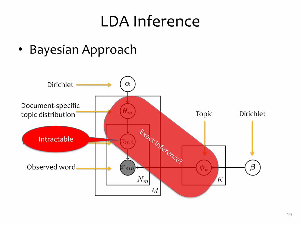
LDA Inference
• Bayesian Approach054055056057058059060061062063064065066067068069070071072073074075076077078079080081082083084085086087088089090091092093094095096097098099100101102103104105106107
M
Nm K
xmn
zmn
⇤m
�
⌅k ⇥
Figure 1: The graphical model for the SCTM.
2 SCTM
A Product of Experts (PoE) [1] model p(x|⌅1, . . . ,⌅C) =QC
c=1 ⇥cxPVv=1
QCc=1 ⇥cv
, where there are C
components, and the summation in the denominator is over all possible feature types.
Latent Dirichlet allocation generative process
For each topic k ⇥ {1, . . . , K}:�k � Dir(�) [draw distribution over words]
For each document m ⇥ {1, . . . , M}✓m � Dir(↵) [draw distribution over topics]For each word n ⇥ {1, . . . , Nm}
zmn � Mult(1, ✓m) [draw topic]xmn � �zmi
[draw word]
The Finite IBP model generative process
For each component c ⇥ {1, . . . , C}: [columns]
�c � Beta( �C , 1) [draw probability of component c]
For each topic k ⇥ {1, . . . , K}: [rows]bkc � Bernoulli(�c)[draw whether topic includes cth component in its PoE]
2.1 PoE
p(x|⌅1, . . . ,⌅C) =⇥C
c=1 ⇤cx�Vv=1
⇥Cc=1 ⇤cv
(2)
2.2 IBP
Latent Dirichlet allocation generative process
For each topic k ⇥ {1, . . . , K}:�k � Dir(�) [draw distribution over words]
For each document m ⇥ {1, . . . , M}✓m � Dir(↵) [draw distribution over topics]For each word n ⇥ {1, . . . , Nm}
zmn � Mult(1, ✓m) [draw topic]xmn � �zmi
[draw word]
The Beta-Bernoulli model generative process
For each feature c ⇥ {1, . . . , C}: [columns]
�c � Beta( �C , 1)
For each class k ⇥ {1, . . . , K}: [rows]bkc � Bernoulli(�c)
2.3 Shared Components Topic Models
Generative process We can now present the formal generative process for the SCTM. For eachof the C shared components, we generate a distribution ⌅c over the V words from a Dirichletparametrized by ⇥. Next, we generate a K � C binary matrix using the finite IBP prior. We selectthe probability ⇥c of each component c being on (bkc = 1) from a Beta distribution parametrizedby �/C. We then sample K topics (rows of the matrix), which combine component distributions,where each position bkc is drawn from a Bernoulli parameterized by ⇥c. These components and the
2
Dirichlet
Document-specific topic distribution
Topic assignment
Observed word
Topic Dirichlet
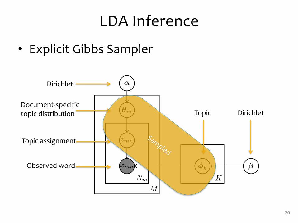
Exact Inference?
Intractable
19
LDA Inference
• Explicit Gibbs Sampler054055056057058059060061062063064065066067068069070071072073074075076077078079080081082083084085086087088089090091092093094095096097098099100101102103104105106107
M
Nm K
xmn
zmn
⇤m
�
⌅k ⇥
Figure 1: The graphical model for the SCTM.
2 SCTM
A Product of Experts (PoE) [1] model p(x|⌅1, . . . ,⌅C) =QC
c=1 ⇥cxPVv=1
QCc=1 ⇥cv
, where there are C
components, and the summation in the denominator is over all possible feature types.
Latent Dirichlet allocation generative process
For each topic k ⇥ {1, . . . , K}:�k � Dir(�) [draw distribution over words]
For each document m ⇥ {1, . . . , M}✓m � Dir(↵) [draw distribution over topics]For each word n ⇥ {1, . . . , Nm}
zmn � Mult(1, ✓m) [draw topic]xmn � �zmi
[draw word]
The Finite IBP model generative process
For each component c ⇥ {1, . . . , C}: [columns]
�c � Beta( �C , 1) [draw probability of component c]
For each topic k ⇥ {1, . . . , K}: [rows]bkc � Bernoulli(�c)[draw whether topic includes cth component in its PoE]
2.1 PoE
p(x|⌅1, . . . ,⌅C) =⇥C
c=1 ⇤cx�Vv=1
⇥Cc=1 ⇤cv
(2)
2.2 IBP
Latent Dirichlet allocation generative process
For each topic k ⇥ {1, . . . , K}:�k � Dir(�) [draw distribution over words]
For each document m ⇥ {1, . . . , M}✓m � Dir(↵) [draw distribution over topics]For each word n ⇥ {1, . . . , Nm}
zmn � Mult(1, ✓m) [draw topic]xmn � �zmi
[draw word]
The Beta-Bernoulli model generative process
For each feature c ⇥ {1, . . . , C}: [columns]
�c � Beta( �C , 1)
For each class k ⇥ {1, . . . , K}: [rows]bkc � Bernoulli(�c)
2.3 Shared Components Topic Models
Generative process We can now present the formal generative process for the SCTM. For eachof the C shared components, we generate a distribution ⌅c over the V words from a Dirichletparametrized by ⇥. Next, we generate a K � C binary matrix using the finite IBP prior. We selectthe probability ⇥c of each component c being on (bkc = 1) from a Beta distribution parametrizedby �/C. We then sample K topics (rows of the matrix), which combine component distributions,where each position bkc is drawn from a Bernoulli parameterized by ⇥c. These components and the
2
Dirichlet
Document-specific topic distribution
Topic assignment
Observed word
Topic Dirichlet
Sampled
20
LDA Inference
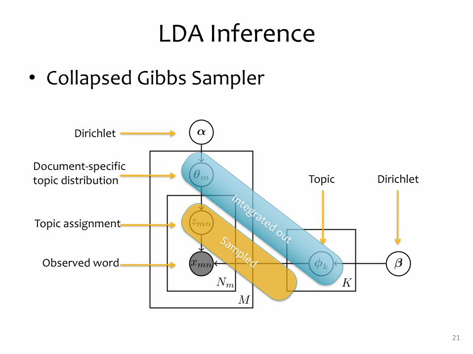
• Collapsed Gibbs Sampler054055056057058059060061062063064065066067068069070071072073074075076077078079080081082083084085086087088089090091092093094095096097098099100101102103104105106107
M
Nm K
xmn
zmn
⇤m
�
⌅k ⇥
Figure 1: The graphical model for the SCTM.
2 SCTM
A Product of Experts (PoE) [1] model p(x|⌅1, . . . ,⌅C) =QC
c=1 ⇥cxPVv=1
QCc=1 ⇥cv
, where there are C
components, and the summation in the denominator is over all possible feature types.
Latent Dirichlet allocation generative process
For each topic k ⇥ {1, . . . , K}:�k � Dir(�) [draw distribution over words]
For each document m ⇥ {1, . . . , M}✓m � Dir(↵) [draw distribution over topics]For each word n ⇥ {1, . . . , Nm}
zmn � Mult(1, ✓m) [draw topic]xmn � �zmi
[draw word]
The Finite IBP model generative process
For each component c ⇥ {1, . . . , C}: [columns]
�c � Beta( �C , 1) [draw probability of component c]
For each topic k ⇥ {1, . . . , K}: [rows]bkc � Bernoulli(�c)[draw whether topic includes cth component in its PoE]
2.1 PoE
p(x|⌅1, . . . ,⌅C) =⇥C
c=1 ⇤cx�Vv=1
⇥Cc=1 ⇤cv
(2)
2.2 IBP
Latent Dirichlet allocation generative process
For each topic k ⇥ {1, . . . , K}:�k � Dir(�) [draw distribution over words]
For each document m ⇥ {1, . . . , M}✓m � Dir(↵) [draw distribution over topics]For each word n ⇥ {1, . . . , Nm}
zmn � Mult(1, ✓m) [draw topic]xmn � �zmi
[draw word]
The Beta-Bernoulli model generative process
For each feature c ⇥ {1, . . . , C}: [columns]
�c � Beta( �C , 1)
For each class k ⇥ {1, . . . , K}: [rows]bkc � Bernoulli(�c)
2.3 Shared Components Topic Models
Generative process We can now present the formal generative process for the SCTM. For eachof the C shared components, we generate a distribution ⌅c over the V words from a Dirichletparametrized by ⇥. Next, we generate a K � C binary matrix using the finite IBP prior. We selectthe probability ⇥c of each component c being on (bkc = 1) from a Beta distribution parametrizedby �/C. We then sample K topics (rows of the matrix), which combine component distributions,where each position bkc is drawn from a Bernoulli parameterized by ⇥c. These components and the
2
Dirichlet
Document-specific topic distribution
Topic assignment
Observed word
Topic DirichletIntegrated outSampled
21
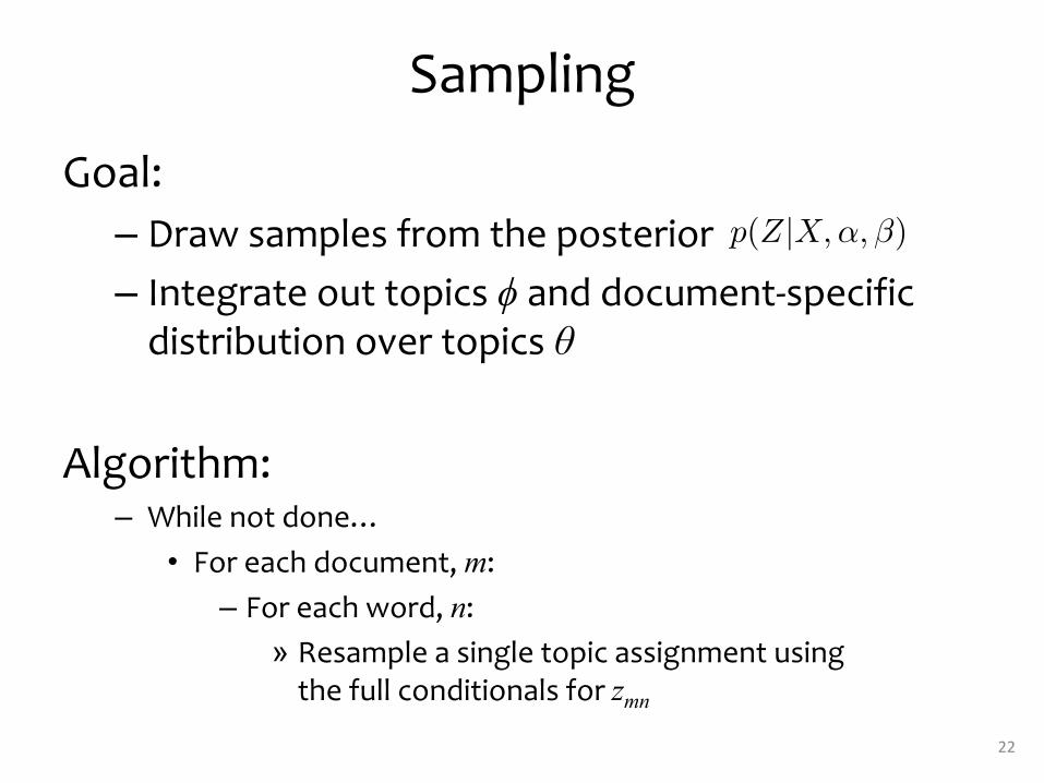
Sampling
Goal:– Draw samples from the posterior – Integrate out topics ϕ and document-specific
distribution over topics θ
Algorithm:– While not done…
• For each document, m:– For each word, n:
» Resample a single topic assignment using the full conditionals for zmn
p(Z|X,↵, �)
22
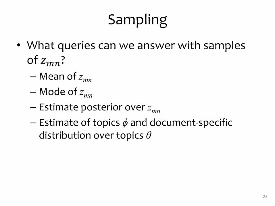
Sampling
• What queries can we answer with samples of !"#?– Mean of zmn– Mode of zmn– Estimate posterior over zmn– Estimate of topics ϕ and document-specific
distribution over topics θ
23
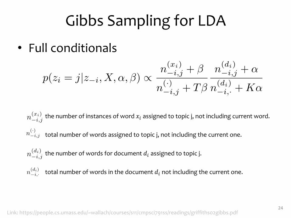
Gibbs Sampling for LDA
• Full conditionals
Link: https://people.cs.umass.edu/~wallach/courses/s11/cmpsci791ss/readings/griffiths02gibbs.pdf
the number of instances of word !" assigned to topic j, not including current word.
total number of words assigned to topic j, not including the current one.
the number of words for document #" assigned to topic j.
total number of words in the document #" not including the current one.
p(zi = j|z�i, X,↵,�) /n(xi)�i,j + �
n(·)�i,j + T�
n(di)�i,j + ↵
n(di)�i,· +K↵
<latexit sha1_base64="hfIqb911FmJq3kvK18JsQedTUiA=">AAAConicbVFda9swFJW9bu3SfWTb414uDYWUZcEehW0Pg9LBKPShKWvaQJwZWZYbtbIkJHk09fzH9jP21n9T2fEga3ZB6HDPuUfSUaI4MzYI7jz/0cbjJ5tbTzvbz56/eNl99frcyEITOiaSSz1JsKGcCTq2zHI6UZriPOH0Irn+WvMXP6k2TIozu1B0luNLwTJGsHWtuPtb9W9jBl/gCn7BbVy+Z9VgMoAIczXHbk+oxXsQKS2VlRBlGpNS1LLBVfWj7N/EbK+Cd0tdVQLAChmRVNqGhrOlAqCCdZP0r0lz6IpLY7CqgONWVBvF3V4wDJqCdRC2oIfaGsXdP1EqSZFTYQnHxkzDQNlZibVlhNOqExWGKkyu8SWdOihwTs2sbDKuYNd1UsikdktYaLqrEyXOjVnkiVPm2M7NQ65u/o+bFjb7NCuZUIWlgiwPygoOLu76wyBlmhLLFw5gopm7K5A5dhFa960dF0L48MnrYPxh+HkYnu73Dg7bNLbQW7SD+ihEH9EBOkIjNEbEA++bd+KN/F3/2D/1vy+lvtfOvEH/lB/dAzAyyBg=</latexit><latexit sha1_base64="hfIqb911FmJq3kvK18JsQedTUiA=">AAAConicbVFda9swFJW9bu3SfWTb414uDYWUZcEehW0Pg9LBKPShKWvaQJwZWZYbtbIkJHk09fzH9jP21n9T2fEga3ZB6HDPuUfSUaI4MzYI7jz/0cbjJ5tbTzvbz56/eNl99frcyEITOiaSSz1JsKGcCTq2zHI6UZriPOH0Irn+WvMXP6k2TIozu1B0luNLwTJGsHWtuPtb9W9jBl/gCn7BbVy+Z9VgMoAIczXHbk+oxXsQKS2VlRBlGpNS1LLBVfWj7N/EbK+Cd0tdVQLAChmRVNqGhrOlAqCCdZP0r0lz6IpLY7CqgONWVBvF3V4wDJqCdRC2oIfaGsXdP1EqSZFTYQnHxkzDQNlZibVlhNOqExWGKkyu8SWdOihwTs2sbDKuYNd1UsikdktYaLqrEyXOjVnkiVPm2M7NQ65u/o+bFjb7NCuZUIWlgiwPygoOLu76wyBlmhLLFw5gopm7K5A5dhFa960dF0L48MnrYPxh+HkYnu73Dg7bNLbQW7SD+ihEH9EBOkIjNEbEA++bd+KN/F3/2D/1vy+lvtfOvEH/lB/dAzAyyBg=</latexit><latexit sha1_base64="hfIqb911FmJq3kvK18JsQedTUiA=">AAAConicbVFda9swFJW9bu3SfWTb414uDYWUZcEehW0Pg9LBKPShKWvaQJwZWZYbtbIkJHk09fzH9jP21n9T2fEga3ZB6HDPuUfSUaI4MzYI7jz/0cbjJ5tbTzvbz56/eNl99frcyEITOiaSSz1JsKGcCTq2zHI6UZriPOH0Irn+WvMXP6k2TIozu1B0luNLwTJGsHWtuPtb9W9jBl/gCn7BbVy+Z9VgMoAIczXHbk+oxXsQKS2VlRBlGpNS1LLBVfWj7N/EbK+Cd0tdVQLAChmRVNqGhrOlAqCCdZP0r0lz6IpLY7CqgONWVBvF3V4wDJqCdRC2oIfaGsXdP1EqSZFTYQnHxkzDQNlZibVlhNOqExWGKkyu8SWdOihwTs2sbDKuYNd1UsikdktYaLqrEyXOjVnkiVPm2M7NQ65u/o+bFjb7NCuZUIWlgiwPygoOLu76wyBlmhLLFw5gopm7K5A5dhFa960dF0L48MnrYPxh+HkYnu73Dg7bNLbQW7SD+ihEH9EBOkIjNEbEA++bd+KN/F3/2D/1vy+lvtfOvEH/lB/dAzAyyBg=</latexit><latexit sha1_base64="hfIqb911FmJq3kvK18JsQedTUiA=">AAAConicbVFda9swFJW9bu3SfWTb414uDYWUZcEehW0Pg9LBKPShKWvaQJwZWZYbtbIkJHk09fzH9jP21n9T2fEga3ZB6HDPuUfSUaI4MzYI7jz/0cbjJ5tbTzvbz56/eNl99frcyEITOiaSSz1JsKGcCTq2zHI6UZriPOH0Irn+WvMXP6k2TIozu1B0luNLwTJGsHWtuPtb9W9jBl/gCn7BbVy+Z9VgMoAIczXHbk+oxXsQKS2VlRBlGpNS1LLBVfWj7N/EbK+Cd0tdVQLAChmRVNqGhrOlAqCCdZP0r0lz6IpLY7CqgONWVBvF3V4wDJqCdRC2oIfaGsXdP1EqSZFTYQnHxkzDQNlZibVlhNOqExWGKkyu8SWdOihwTs2sbDKuYNd1UsikdktYaLqrEyXOjVnkiVPm2M7NQ65u/o+bFjb7NCuZUIWlgiwPygoOLu76wyBlmhLLFw5gopm7K5A5dhFa960dF0L48MnrYPxh+HkYnu73Dg7bNLbQW7SD+ihEH9EBOkIjNEbEA++bd+KN/F3/2D/1vy+lvtfOvEH/lB/dAzAyyBg=</latexit>
24
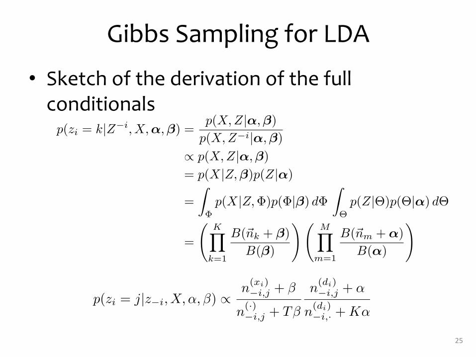
Gibbs Sampling for LDA
• Sketch of the derivation of the full conditionals
054055056057058059060061062063064065066067068069070071072073074075076077078079080081082083084085086087088089090091092093094095096097098099100101102103104105106107
For each topic k ⇤ {1, . . . ,K}:⌅k � Dir(⇥) [draw distribution over words]
For each document m ⇤ {1, . . . ,M}⇤m � Dir(�) [draw distribution over topics]For each word n ⇤ {1, . . . , Nm}
zmn � Mult(1,⇤m) [draw topic assignment]xmn � ⌅zmi
[draw word]
M
Nm K
xmn
zmn
⇤m
�
⌅k ⇥
Figure 1: The graphical model for the SCTM.
LDA Full Conditionals:
p(zi = k|Z�i, X,�,⇥) =p(X, Z|�,⇥)
p(X, Z�i|�,⇥)(2)
⇥ p(X, Z|�,⇥) (3)= p(X|Z,⇥)p(Z|�) (4)
=⇧
⇥p(X|Z,⇥)p(⇥|⇥) d⇥
⇧
�p(Z|�)p(�|�) d� (5)
=
�K⌅
k=1
B(⇤nk + ⇥)B(⇥)
⇥ �M⌅
m=1
B(⇤nm + �)B(�)
⇥(6)
=n�i
kt + ⇥t⇤Tv=1 n�i
kv + ⇥v
·n�i
mk + �k⇤Kj=1 n�i
mj + �j
(7)
where t, m are given by i
(8)
Why conjugacy is great:
2
p(zi = j|z�i, X,↵,�) /n(xi)�i,j + �
n(·)�i,j + T�
n(di)�i,j + ↵
n(di)�i,· +K↵
<latexit sha1_base64="hfIqb911FmJq3kvK18JsQedTUiA=">AAAConicbVFda9swFJW9bu3SfWTb414uDYWUZcEehW0Pg9LBKPShKWvaQJwZWZYbtbIkJHk09fzH9jP21n9T2fEga3ZB6HDPuUfSUaI4MzYI7jz/0cbjJ5tbTzvbz56/eNl99frcyEITOiaSSz1JsKGcCTq2zHI6UZriPOH0Irn+WvMXP6k2TIozu1B0luNLwTJGsHWtuPtb9W9jBl/gCn7BbVy+Z9VgMoAIczXHbk+oxXsQKS2VlRBlGpNS1LLBVfWj7N/EbK+Cd0tdVQLAChmRVNqGhrOlAqCCdZP0r0lz6IpLY7CqgONWVBvF3V4wDJqCdRC2oIfaGsXdP1EqSZFTYQnHxkzDQNlZibVlhNOqExWGKkyu8SWdOihwTs2sbDKuYNd1UsikdktYaLqrEyXOjVnkiVPm2M7NQ65u/o+bFjb7NCuZUIWlgiwPygoOLu76wyBlmhLLFw5gopm7K5A5dhFa960dF0L48MnrYPxh+HkYnu73Dg7bNLbQW7SD+ihEH9EBOkIjNEbEA++bd+KN/F3/2D/1vy+lvtfOvEH/lB/dAzAyyBg=</latexit><latexit sha1_base64="hfIqb911FmJq3kvK18JsQedTUiA=">AAAConicbVFda9swFJW9bu3SfWTb414uDYWUZcEehW0Pg9LBKPShKWvaQJwZWZYbtbIkJHk09fzH9jP21n9T2fEga3ZB6HDPuUfSUaI4MzYI7jz/0cbjJ5tbTzvbz56/eNl99frcyEITOiaSSz1JsKGcCTq2zHI6UZriPOH0Irn+WvMXP6k2TIozu1B0luNLwTJGsHWtuPtb9W9jBl/gCn7BbVy+Z9VgMoAIczXHbk+oxXsQKS2VlRBlGpNS1LLBVfWj7N/EbK+Cd0tdVQLAChmRVNqGhrOlAqCCdZP0r0lz6IpLY7CqgONWVBvF3V4wDJqCdRC2oIfaGsXdP1EqSZFTYQnHxkzDQNlZibVlhNOqExWGKkyu8SWdOihwTs2sbDKuYNd1UsikdktYaLqrEyXOjVnkiVPm2M7NQ65u/o+bFjb7NCuZUIWlgiwPygoOLu76wyBlmhLLFw5gopm7K5A5dhFa960dF0L48MnrYPxh+HkYnu73Dg7bNLbQW7SD+ihEH9EBOkIjNEbEA++bd+KN/F3/2D/1vy+lvtfOvEH/lB/dAzAyyBg=</latexit><latexit sha1_base64="hfIqb911FmJq3kvK18JsQedTUiA=">AAAConicbVFda9swFJW9bu3SfWTb414uDYWUZcEehW0Pg9LBKPShKWvaQJwZWZYbtbIkJHk09fzH9jP21n9T2fEga3ZB6HDPuUfSUaI4MzYI7jz/0cbjJ5tbTzvbz56/eNl99frcyEITOiaSSz1JsKGcCTq2zHI6UZriPOH0Irn+WvMXP6k2TIozu1B0luNLwTJGsHWtuPtb9W9jBl/gCn7BbVy+Z9VgMoAIczXHbk+oxXsQKS2VlRBlGpNS1LLBVfWj7N/EbK+Cd0tdVQLAChmRVNqGhrOlAqCCdZP0r0lz6IpLY7CqgONWVBvF3V4wDJqCdRC2oIfaGsXdP1EqSZFTYQnHxkzDQNlZibVlhNOqExWGKkyu8SWdOihwTs2sbDKuYNd1UsikdktYaLqrEyXOjVnkiVPm2M7NQ65u/o+bFjb7NCuZUIWlgiwPygoOLu76wyBlmhLLFw5gopm7K5A5dhFa960dF0L48MnrYPxh+HkYnu73Dg7bNLbQW7SD+ihEH9EBOkIjNEbEA++bd+KN/F3/2D/1vy+lvtfOvEH/lB/dAzAyyBg=</latexit><latexit sha1_base64="hfIqb911FmJq3kvK18JsQedTUiA=">AAAConicbVFda9swFJW9bu3SfWTb414uDYWUZcEehW0Pg9LBKPShKWvaQJwZWZYbtbIkJHk09fzH9jP21n9T2fEga3ZB6HDPuUfSUaI4MzYI7jz/0cbjJ5tbTzvbz56/eNl99frcyEITOiaSSz1JsKGcCTq2zHI6UZriPOH0Irn+WvMXP6k2TIozu1B0luNLwTJGsHWtuPtb9W9jBl/gCn7BbVy+Z9VgMoAIczXHbk+oxXsQKS2VlRBlGpNS1LLBVfWj7N/EbK+Cd0tdVQLAChmRVNqGhrOlAqCCdZP0r0lz6IpLY7CqgONWVBvF3V4wDJqCdRC2oIfaGsXdP1EqSZFTYQnHxkzDQNlZibVlhNOqExWGKkyu8SWdOihwTs2sbDKuYNd1UsikdktYaLqrEyXOjVnkiVPm2M7NQ65u/o+bFjb7NCuZUIWlgiwPygoOLu76wyBlmhLLFw5gopm7K5A5dhFa960dF0L48MnrYPxh+HkYnu73Dg7bNLbQW7SD+ihEH9EBOkIjNEbEA++bd+KN/F3/2D/1vy+lvtfOvEH/lB/dAzAyyBg=</latexit>
25

MARKOV CHAINSDefinitions and Theoretical Justification for MCMC
28
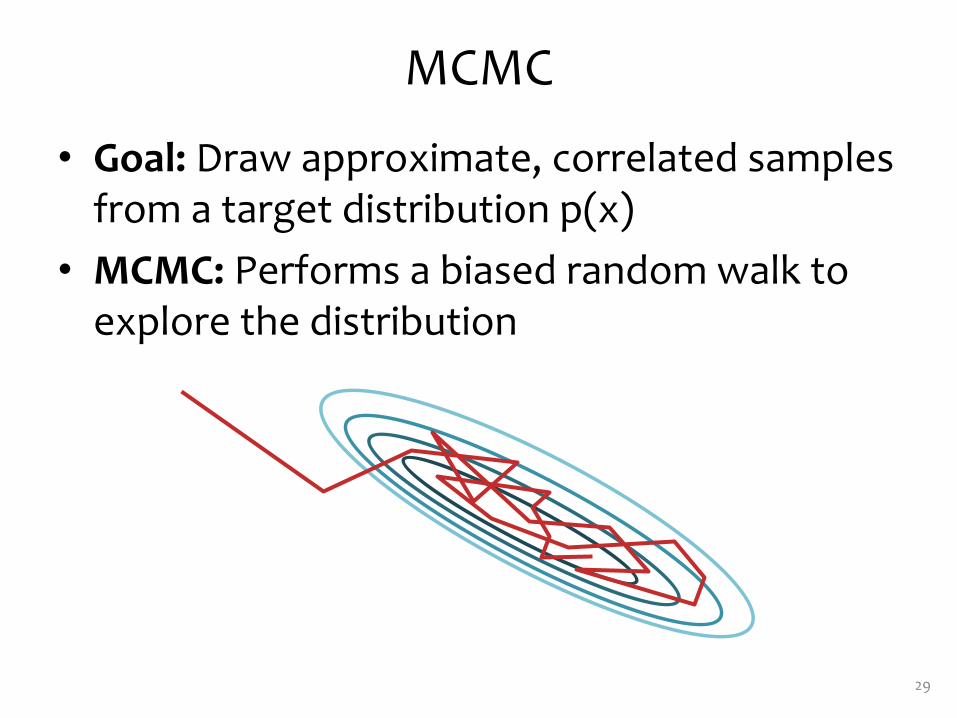
MCMC
• Goal: Draw approximate, correlated samples from a target distribution p(x)
• MCMC: Performs a biased random walk to explore the distribution
29
Simulations of MCMC
30
Visualization of Metroplis-Hastings, Gibbs Sampling, and Hamiltonian MCMC:
https://www.youtube.com/watch?v=Vv3f0QNWvWQ
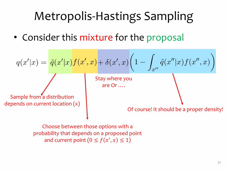
Metropolis-Hastings Sampling
• Consider this mixture for the proposal
31
Stay where you are Or ….
Sample from a distribution depends on current location (x)
Choose between those options with a probability that depends on a proposed point
and current point (0 ≤ # $%, $ ≤ 1)
Of course! It should be a proper density!
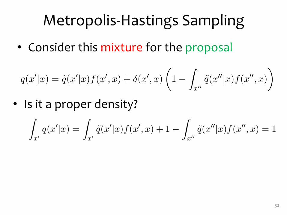
Metropolis-Hastings Sampling
• Consider this mixture for the proposal
32
• Is it a proper density?
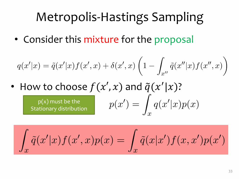
Metropolis-Hastings Sampling
• Consider this mixture for the proposal
33
• How to choose !(#′, #) and '((#)|#)?p(x) must be the
Stationary distribution
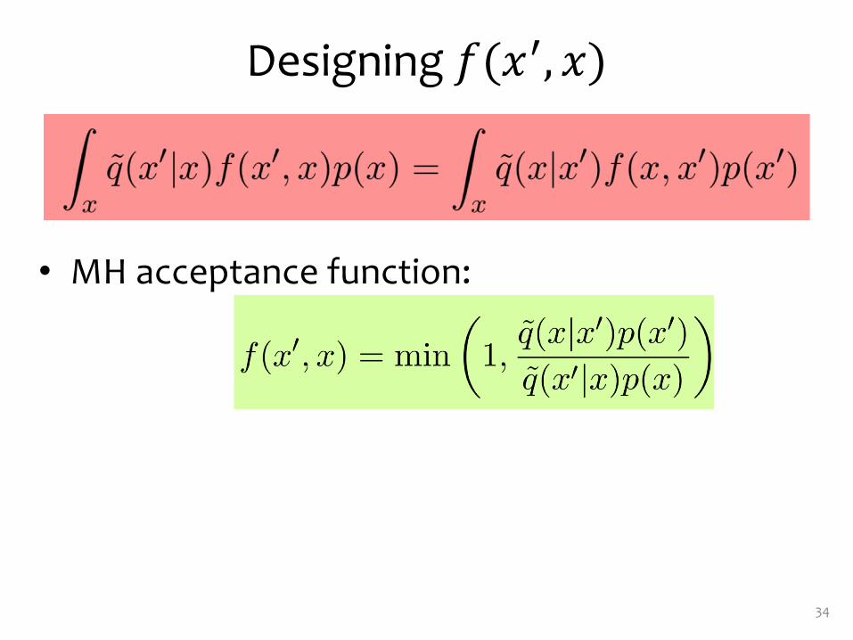
Designing !(#$, #)
34
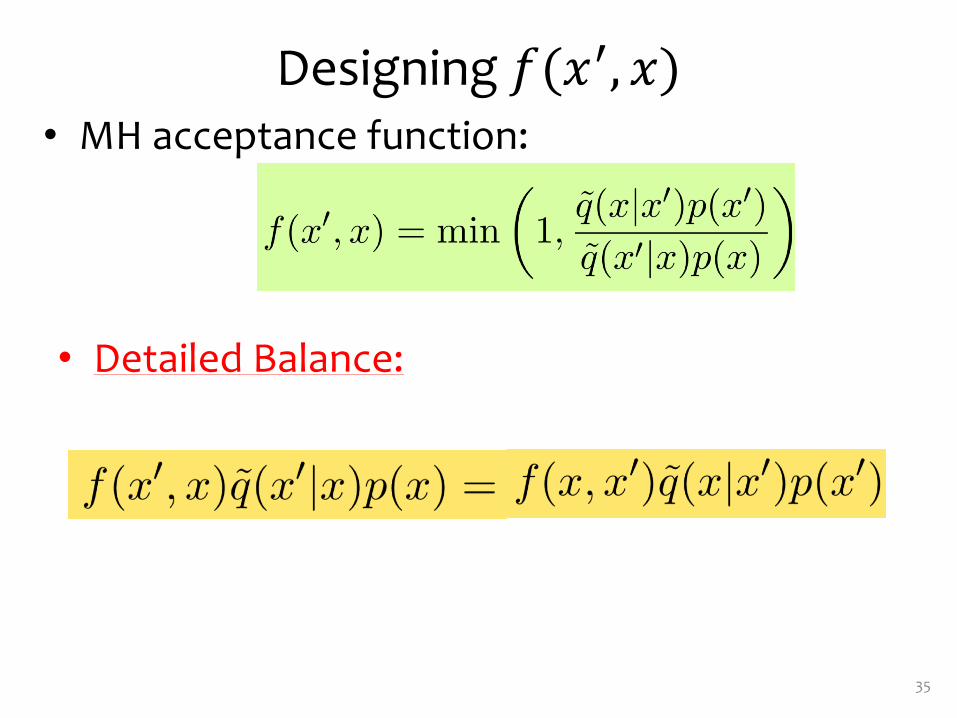
• MH acceptance function:
Designing !(#$, #)
35
• MH acceptance function:
• Detailed Balance:
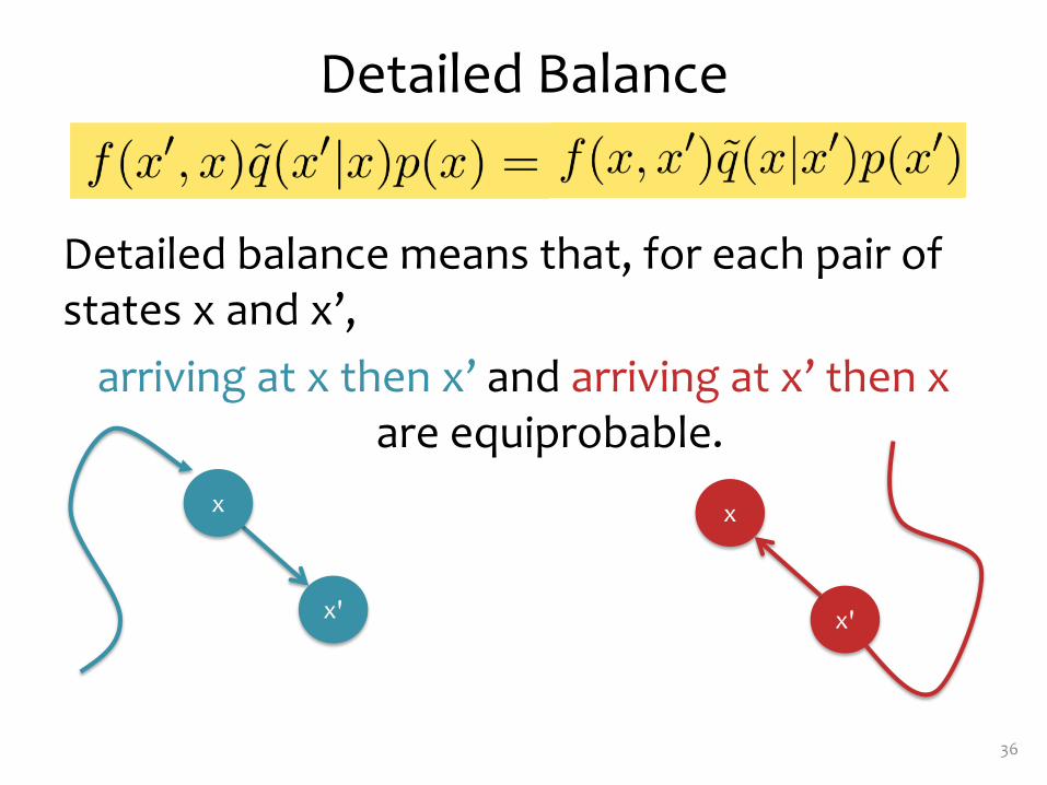
Detailed Balance
Detailed balance means that, for each pair of states x and x’,
arriving at x then x’ and arriving at x’ then xare equiprobable.
36
x
x'
x
x'
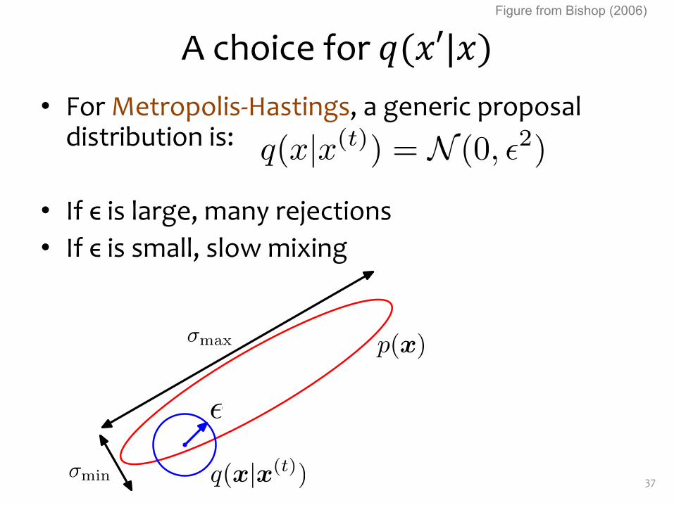
A choice for !(#′|#)• For Metropolis-Hastings, a generic proposal
distribution is:
• If ϵ is large, many rejections• If ϵ is small, slow mixing
37
�max
�min
⇢✏
p(x)
q(x|x(t))
Figure from Bishop (2006)
q(x|x(t)) = N (0, ✏2)
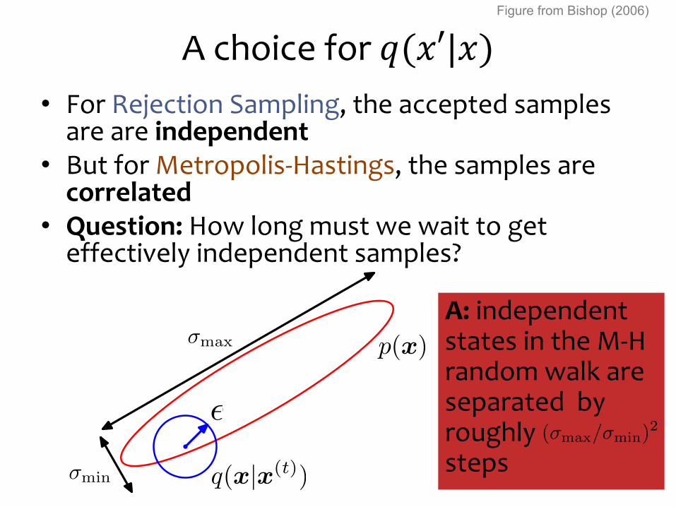
A choice for !(#′|#)• For Rejection Sampling, the accepted samples
are are independent• But for Metropolis-Hastings, the samples are correlated
• Question: How long must we wait to get effectively independent samples?
38
�max
�min
⇢✏
p(x)
q(x|x(t))
A: independent states in the M-H random walk are separated by roughlysteps
(�max/�min)2
Figure from Bishop (2006)
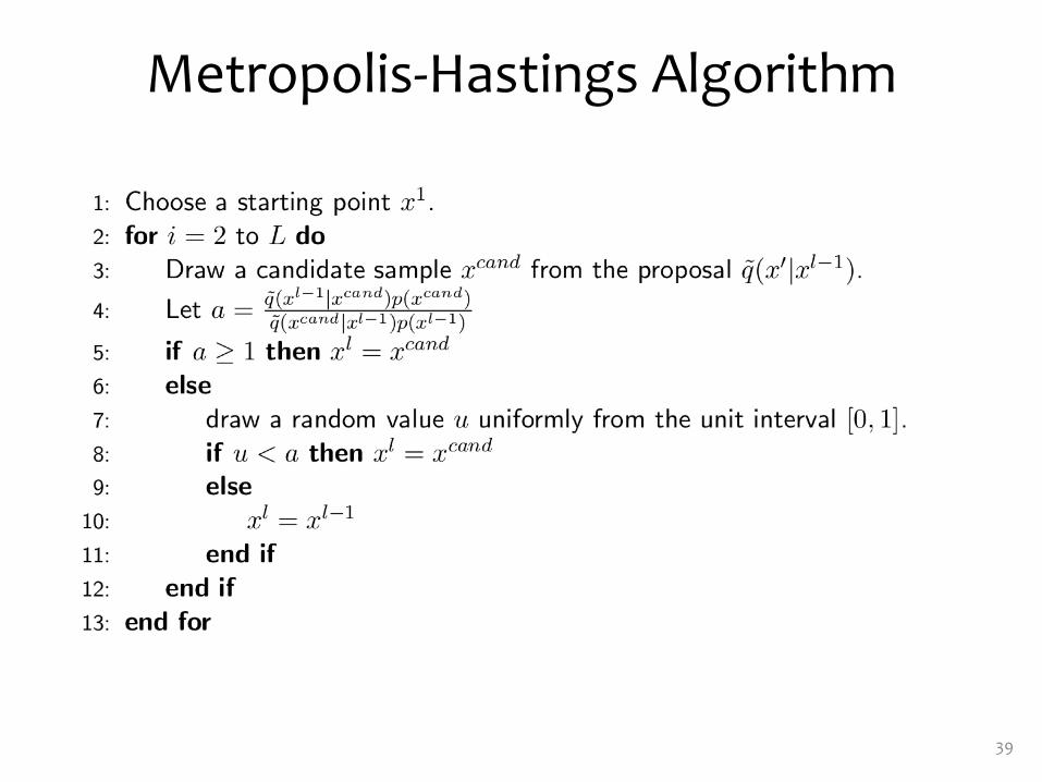
Metropolis-Hastings Algorithm
39
Practical Issues• Question: Is it better to move along one dimension
or many?
• Answer: For Metropolis-Hasings, it is sometimes better to sample one dimension at a time– Q: Given a sequence of 1D proposals, compare rate of
movement for one-at-a-time vs. concatenation.
• Answer: For Gibbs Sampling, sometimes better to sample a block of variables at a time– Q: When is it tractable to sample a block of variables?
42
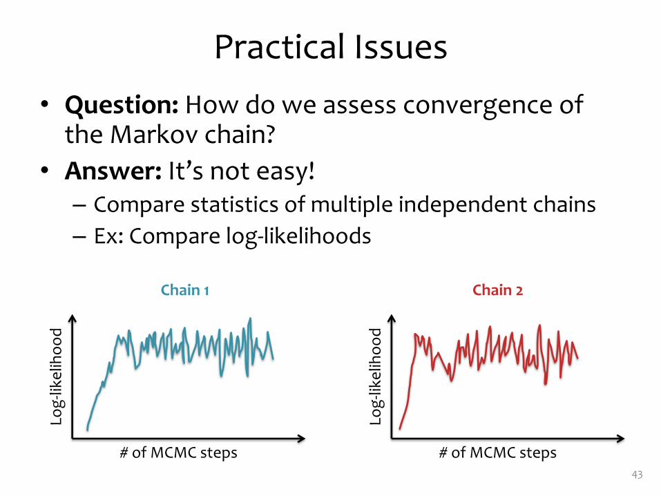
Practical Issues• Question: How do we assess convergence of
the Markov chain?• Answer: It’s not easy!– Compare statistics of multiple independent chains– Ex: Compare log-likelihoods
43
# of MCMC steps
Log-
likel
ihoo
d
# of MCMC steps
Log-
likel
ihoo
d
Chain 1 Chain 2
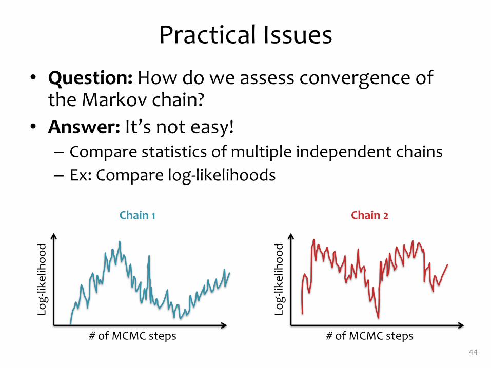
Practical Issues• Question: How do we assess convergence of
the Markov chain?• Answer: It’s not easy!– Compare statistics of multiple independent chains– Ex: Compare log-likelihoods
44
# of MCMC steps
Log-
likel
ihoo
d
# of MCMC steps
Log-
likel
ihoo
d
Chain 1 Chain 2
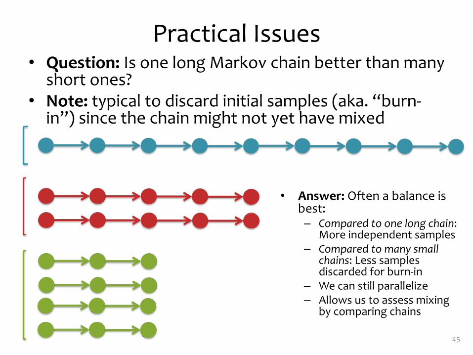
Practical Issues• Question: Is one long Markov chain better than many
short ones?• Note: typical to discard initial samples (aka. “burn-
in”) since the chain might not yet have mixed
45
• Answer: Often a balance is best:– Compared to one long chain:
More independent samples – Compared to many small
chains: Less samples discarded for burn-in
– We can still parallelize– Allows us to assess mixing
by comparing chains