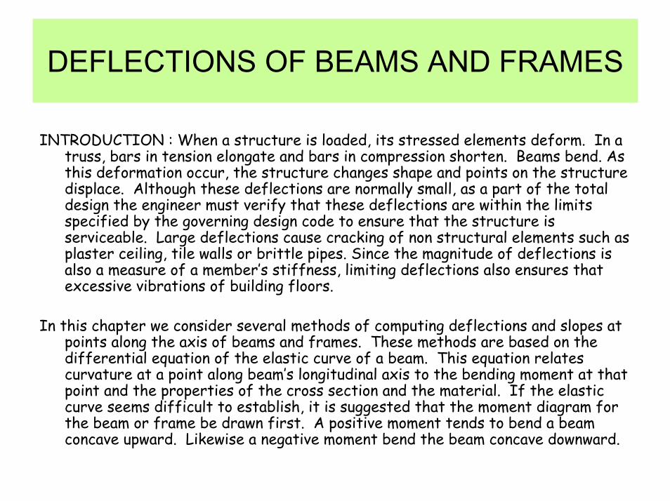
DEFLECTIONS OF BEAMS AND FRAMES

INTRODUCTION : When a structure is loaded, its stressed elements deform. In a truss, bars in tension elongate and bars in compression shorten. Beams bend. As this deformation occur, the structure changes shape and points on the structure displace. Although these deflections are normally small, as a part of the total design the engineer must verify that these deflections are within the limits specified by the governing design code to ensure that the structure is serviceable. Large deflections cause cracking of non structural elements such as plaster ceiling, tile walls or brittle pipes. Since the magnitude of deflections is also a measure of a member’s stiffness, limiting deflections also ensures that excessive vibrations of building floors.

In this chapter we consider several methods of computing deflections and slopes at points along the axis of beams and frames. These methods are based on the differential equation of the elastic curve of a beam. This equation relates curvature at a point along beam’s longitudinal axis to the bending moment at that point and the properties of the cross section and the material. If the elastic curve seems difficult to establish, it is suggested that the moment diagram for the beam or frame be drawn first. A positive moment tends to bend a beam concave upward. Likewise a negative moment bend the beam concave downward.

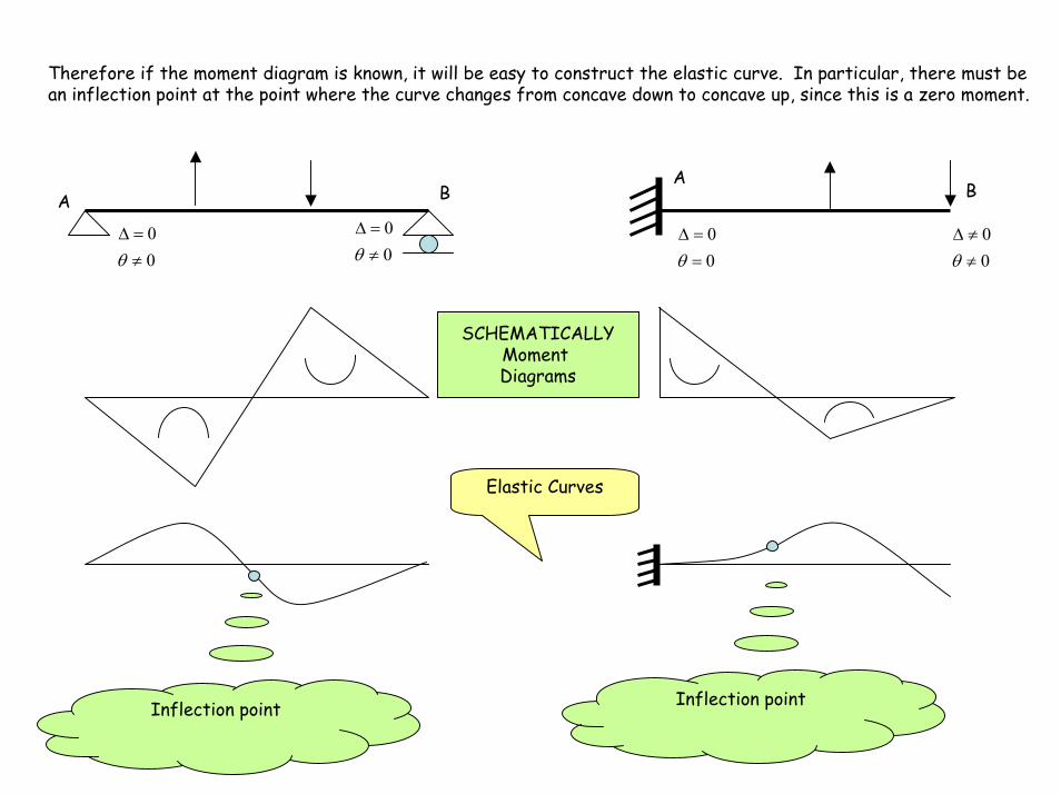
Therefore if the moment diagram is known, it will be easy to construct the elastic curve. In particular, there must be an inflection point at the point where the curve changes from concave down to concave up, since this is a zero moment.

A BA

B

00

≠=∆

θ00

≠=∆

θ 00

==∆

θ 00

≠≠∆

θ

SCHEMATICALLYMoment Diagrams

Elastic Curves

Inflection pointInflection point

DOUBLE INTEGRATION METHOD

The double integration method is a procedure to establish the equations for slope and deflection at points along the elastic curve of a loaded beam. The equations are derived by integrating the differential equation of the elastic curve twice. The method assumes that all deformations are produced by moment.

θ

θd

A

Bds

ρθd

O

Elastic curve

θtan=dxdyThe slope of the curve at point AGEOMETRY OF CURVES

θ=dxdyIf the angles are small, the

slope can be written

From the geometry of triangular segment ABO

A B

dsd =θρ.y

ψθρ

==dsd1

Dividing each side by ds

xx dΘ/ds represents the change in slope per unit length

of distance along the curve, is called curvature and denoted by symbol Ψ. Since slopes are small in actual beams ds=dx we can express the curvature,

dx

Line tangent at B

ρθψ 1==

dxd

Differentiating both sides of the second equation

2

2

dxyd

dxd

=θ

Line tangent at A

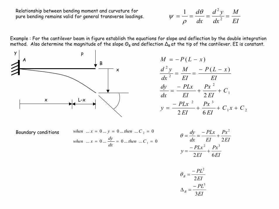
Relationship between bending moment and curvature for pure bending remains valid for general transverse loadings.

EIM

dxyd

dxd

==== 2

21 θρ

ψ

Example : For the cantilever beam in figure establish the equations for slope and deflection by the double integration method. Also determine the magnitude of the slope ΘB and deflection ∆B at the tip of the cantilever. EI is constant.

y P

21

32

1

2

2

2

62

2

)()(

CxCEIPx

EIPLxy

CEIPx

EIPLx

dxdy

EIxLP

EIM

dxyd

xLPM

+++−

=

++−

=

−−==

−−=AB

x

x L-x

0......0...0...

0......0...0...

1

2

===

===

Cthendxdyxwhen

CthenyxwhenBoundary conditions

EIPLEIPL

EIPx

EIPLxy

EIPx

EIPLx

dxdy

B

B

3

2

62

2

3

2

32

2

−=∆

−=

+−

=

+−

==

θ

θ

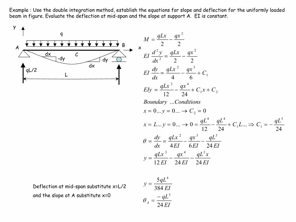
Example : Use the double integration method, establish the equations for slope and deflection for the uniformly loaded beam in figure. Evaluate the deflection at mid-span and the slope at support A. EI is constant.

yq

EIqLEIqLy

EIxqL

EIqx

EIqLxy

EIqL

EIqx

EIqLx

dxdy

qLCLCqLqLyLx

CyxConditionsBoundary

CxCqxqLxEIy

CqxqLxdxdyEI

qxqLxdxydEI

qxqLxM

A 24

3845

242412

2464

24...

24120...0...

0...0...0...

2412

64

22

22

3

4

343

332

3

11

442

21

43

1

32

2

2

2

2

−=

=

−−=

−−==

−=⇒+−=→==

=→==

++−=

+−=

−=

−=

θ

θ

ACdx

-dydx

dy

qL/2

B x

L

Deflection at mid-span substitute x=L/2

and the slope at A substitute x=0

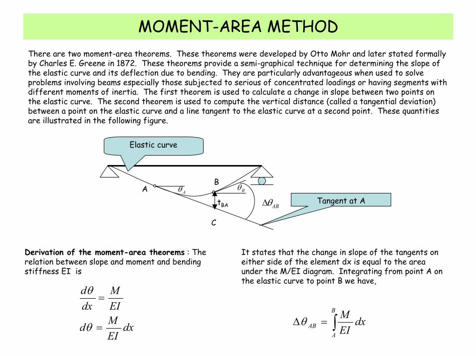
MOMENT-AREA METHODThere are two moment-area theorems. These theorems were developed by Otto Mohr and later stated formally by Charles E. Greene in 1872. These theorems provide a semi-graphical technique for determining the slope of the elastic curve and its deflection due to bending. They are particularly advantageous when used to solve problems involving beams especially those subjected to serious of concentrated loadings or having segments with different moments of inertia. The first theorem is used to calculate a change in slope between two points on the elastic curve. The second theorem is used to compute the vertical distance (called a tangential deviation) between a point on the elastic curve and a line tangent to the elastic curve at a second point. These quantities are illustrated in the following figure.

AB

BθAθ

ABθ∆tBA

C

Elastic curve

Tangent at A

It states that the change in slope of the tangents on either side of the element dx is equal to the area under the M/EI diagram. Integrating from point A on the elastic curve to point B we have,

Derivation of the moment-area theorems : The relation between slope and moment and bending stiffness EI is

dxEIMd

EIM

dxd

=

=

θ

θ

∫=∆B

AAB dx

EIMθ

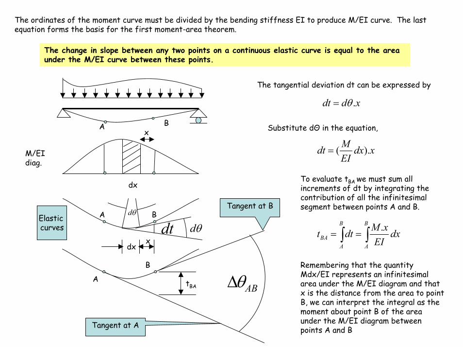
The ordinates of the moment curve must be divided by the bending stiffness EI to produce M/EI curve. The last equation forms the basis for the first moment-area theorem.

The change in slope between any two points on a continuous elastic curve is equal to the area under the M/EI curve between these points.

M/EI diag.

tBAA

B

ABθ∆

dx

θd

θddt

dx

x

x

Tangent at B

Tangent at A

A B

The tangential deviation dt can be expressed by

xddt .θ=

Substitute dΘ in the equation,

xdxEIMdt ).(=

To evaluate tBA we must sum all increments of dt by integrating the contribution of all the infinitesimal segment between points A and B.

∫ ∫==B

A

B

ABA dx

EIxMdtt .

Remembering that the quantity Mdx/EI represents an infinitesimal area under the M/EI diagram and that x is the distance from the area to point B, we can interpret the integral as the moment about point B of the area under the M/EI diagram between points A and B

Elastic curves

BA

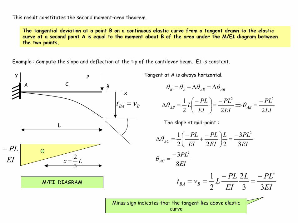
This result constitutes the second moment-area theorem.

The tangential deviation at a point B on a continuous elastic curve from a tangent drawn to the elastic curve at a second point A is equal to the moment about B of the area under the M/EI diagram between the two points.

Example : Compute the slope and deflection at the tip of the cantilever beam. EI is constant.

Tangent at A is always horizontal. y PCA B ABABAB θθθθ ∆=∆+=

x

EIPL

EIPL

EIPLL ABAB 222

1 22 −=⇒

−=

−=∆ θθBBA vt =

The slope at mid-point :L

EIPL

EIPLL

EIPL

EIPL

AC

AC

83

83

2221

2

2

−=

−=

−

+−

=∆

θ

θ

EIPL−

Lx32

=

EIPLL

EIPLLvt BBA 33

221 3−

=−

==M/EI DIAGRAM

Minus sign indicates that the tangent lies above elastic curve

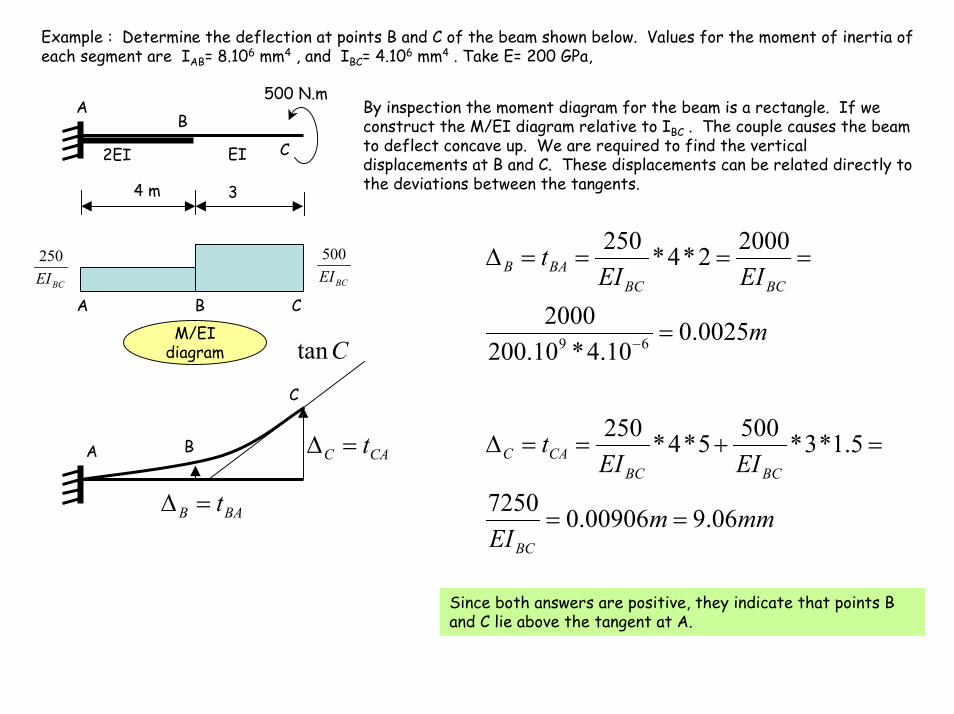
Example : Determine the deflection at points B and C of the beam shown below. Values for the moment of inertia of each segment are IAB= 8.106 mm4 , and IBC= 4.106 mm4 . Take E= 200 GPa,

500 N.m

2EI EI

B

C

A By inspection the moment diagram for the beam is a rectangle. If we construct the M/EI diagram relative to IBC . The couple causes the beam to deflect concave up. We are required to find the vertical displacements at B and C. These displacements can be related directly to the deviations between the tangents. 4 m 3

m

EIEIt

BCBCBAB

0025.010.4*10.200

2000

20002*4*250

69 =

====∆

−

BCEI500

BCEI250

A B C

CAC t=∆

Ctan

C

BAB t=∆

BA

M/EIdiagram

mmmEI

EIEIt

BC

BCBCCAC

06.900906.07250

5.1*3*5005*4*250

==

=+==∆

Since both answers are positive, they indicate that points B and C lie above the tangent at A.

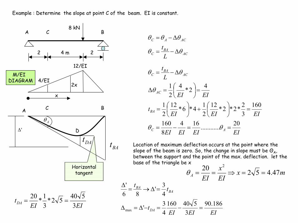
Example : Determine the slope at point C of the beam. EI is constant.

8 kNA BC

ACBA

C

ACAC

Lt θθ

θθθ

∆−=

∆−=

2 24 m

12/EI

EIEIEIEI

EIEIEIt

EIEI

Lt

AC

BA

AC

ACBA

C

20............1648160

16032*2*2*12

214*6*12

21

42*421

==−=

=

+

=

=

=∆

∆−=

θθ

θ

θθ4/EI

M/EI DIAGRAM

x

2x

C BA

Aθ

D

DAt'∆

BAt Location of maximum deflection occurs at the point where the slope of the beam is zero. So, the change in slope must be ΘA, between the support and the point of the max. deflection. let the base of the triangle be x

mxEIx

EIA 47.45220 2

==⇒==θ

EIEIEIt

tt

DA

BABA

186.903

54016043'

43'

86'

max =−=−∆=∆

=∆→=∆

Horizontal tangent

EIEItDA 3

54052*31*20

==

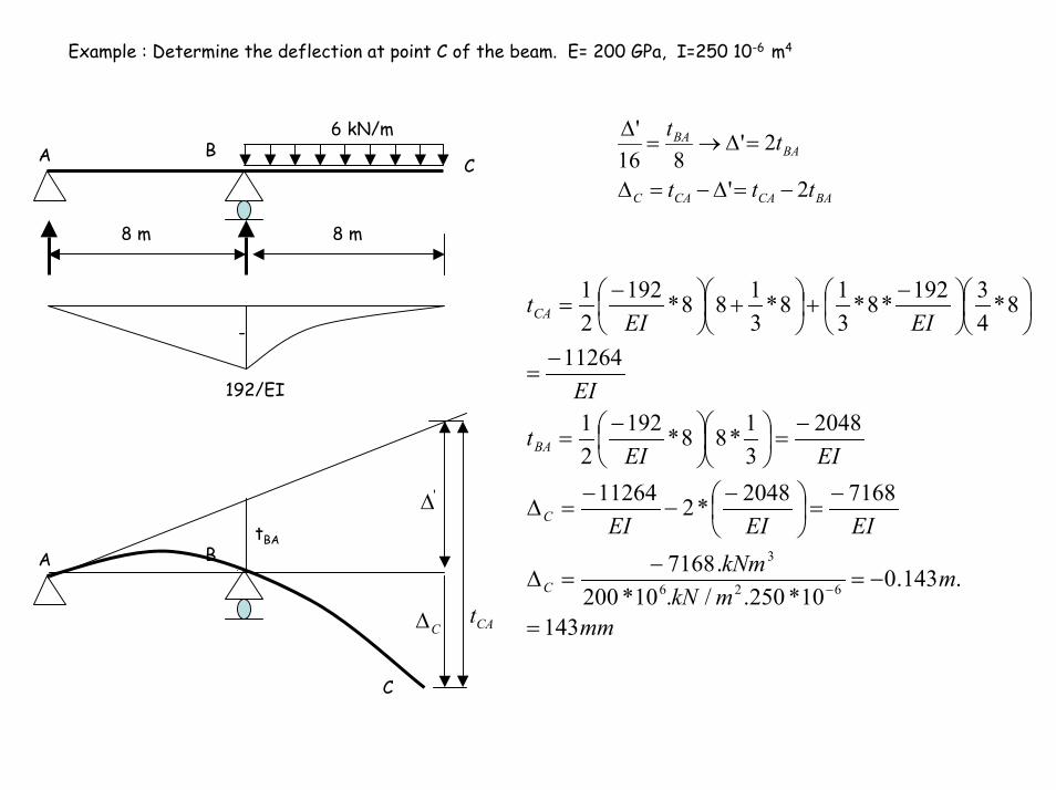
Example : Determine the deflection at point C of the beam. E= 200 GPa, I=250 10-6 m4

BACACAC

BABA

ttt

tt

2'

2'816

'

−=∆−=∆

=∆→=∆6 kN/m

A BC

8 m 8 m

mm

mmkNkNm

EIEIEI

EIEIt

EI

EIEIt

C

C

BA

CA

143

.143.010*250./.10*200

.7168

71682048*211264

204831*88*192

21

11264

8*43192*8*

318*

3188*192

21

626

3

=

−=−

=∆

−=

−−

−=∆

−=

−=

−=

−

+

+

−=

−

-

192/EI

A B

C

tBA

'∆

C∆ CAt

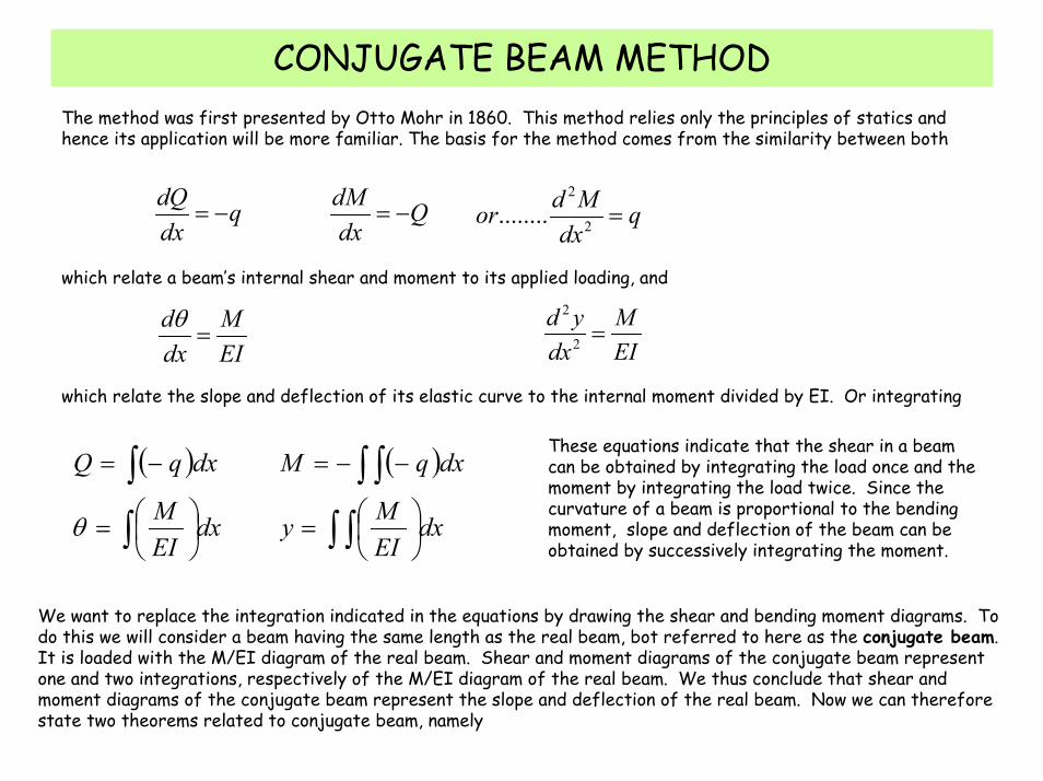
CONJUGATE BEAM METHODThe method was first presented by Otto Mohr in 1860. This method relies only the principles of statics and hence its application will be more familiar. The basis for the method comes from the similarity between both

qdxdQ

−= QdxdM

−= qdxMdor =2

2

........

which relate a beam’s internal shear and moment to its applied loading, and

EIM

dxyd=2

2

EIM

dxd

=θ

which relate the slope and deflection of its elastic curve to the internal moment divided by EI. Or integrating

These equations indicate that the shear in a beam can be obtained by integrating the load once and the moment by integrating the load twice. Since the curvature of a beam is proportional to the bending moment, slope and deflection of the beam can be obtained by successively integrating the moment.

( )

dxEIM

dxqQ

∫

∫

=

−=

θ

( )

∫ ∫

∫ ∫

=

−−=

dxEIMy

dxqM

We want to replace the integration indicated in the equations by drawing the shear and bending moment diagrams. To do this we will consider a beam having the same length as the real beam, bot referred to here as the conjugate beam. It is loaded with the M/EI diagram of the real beam. Shear and moment diagrams of the conjugate beam represent one and two integrations, respectively of the M/EI diagram of the real beam. We thus conclude that shear and moment diagrams of the conjugate beam represent the slope and deflection of the real beam. Now we can therefore state two theorems related to conjugate beam, namely

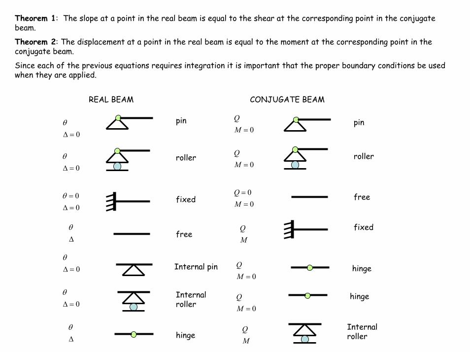
Theorem 1: The slope at a point in the real beam is equal to the shear at the corresponding point in the conjugate beam.

Theorem 2: The displacement at a point in the real beam is equal to the moment at the corresponding point in the conjugate beam.

Since each of the previous equations requires integration it is important that the proper boundary conditions be used when they are applied.

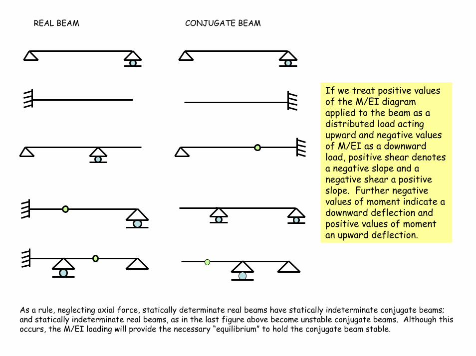
REAL BEAM CONJUGATE BEAM

0=MQ

0=∆θ

0=∆θ

00

=∆=θ

∆θ

0=∆θ

0=∆θ

∆θ

fixed

pin pin

rollerroller0=M

Q

00==

MQ free

fixedMQ

free

0=MQInternal pin hinge

Internal roller

hinge0=M

Q

Internal rollerM

Qhinge

REAL BEAM CONJUGATE BEAM

If we treat positive values of the M/EI diagram applied to the beam as a distributed load acting upward and negative values of M/EI as a downward load, positive shear denotes a negative slope and a negative shear a positive slope. Further negative values of moment indicate a downward deflection and positive values of moment an upward deflection.

As a rule, neglecting axial force, statically determinate real beams have statically indeterminate conjugate beams; and statically indeterminate real beams, as in the last figure above become unstable conjugate beams. Although this occurs, the M/EI loading will provide the necessary “equilibrium” to hold the conjugate beam stable.

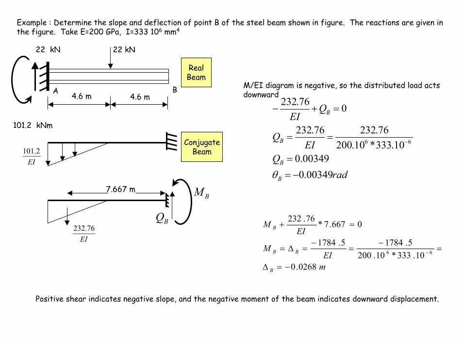
Example : Determine the slope and deflection of point B of the steel beam shown in figure. The reactions are given in the figure. Take E=200 GPa, I=333 106 mm4

22 kN 22 kN

RealBeam

M/EI diagram is negative, so the distributed load acts downward

radQ

EIQ

QEI

B

B

B

B

00349.000349.0

10.333*10.20076.23276.232

076.232

66

−==

==

=+−

−

θ

BA 4.6 m 4.6 m

101.2 kNm

ConjugateBeam

EI2.101

EI76.232

7.667 m

BQ

BM

mEI

M

EIM

B

BB

B

0268.010.333*10.200

5.17845.1784

0667.7*76.232

66

−=∆

=−

=−

=∆=

=+

−

Positive shear indicates negative slope, and the negative moment of the beam indicates downward displacement.

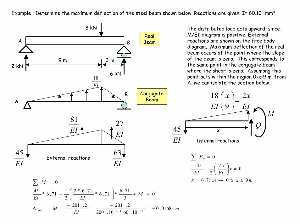
Example : Determine the maximum deflection of the steel beam shown below. Reactions are given. I= 60.106 mm4

8 kN The distributed load acts upward, since M/EI diagram is positive. External reactions are shown on the free body diagram. Maximum deflection of the real beam occurs at the point where the slope of the beam is zero. This corresponds to the same point in the conjugate beam where the shear is zero. Assumong this point acts within the region 0<x<9 m. from A, we can isolate the section below,

RealBeam

9 m 3 m2 kN

6 kN

A B

EI18

B ConjugateBeamA

EI27

EI81

EI63

EI45

External reactions

EIxx

EI2

918

=

MQ

EI45 x

Internal reactions

mxmx

xEIx

EI

F y

9071.6

022145

0

≤≤→=

=

+

−

=∑

mEI

M

MEIEI

M

0168.010.60*10.200

2.2012.201

0371.6*71.6*71.6*2

2171.6*45

0

66max −=−

=−

==∆

=+

−

=

−

∑

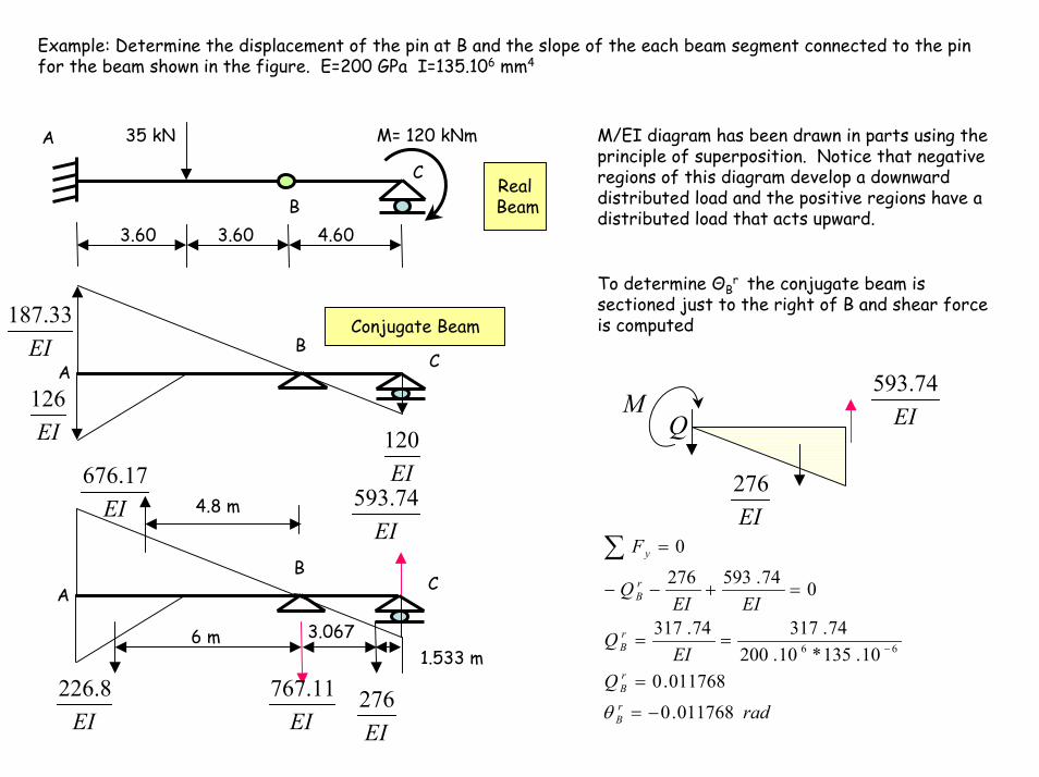
Example: Determine the displacement of the pin at B and the slope of the each beam segment connected to the pin for the beam shown in the figure. E=200 GPa I=135.106 mm4

B

C

M= 120 kNm

3.60 3.60 4.60

RealBeam

35 kN M/EI diagram has been drawn in parts using the principle of superposition. Notice that negative regions of this diagram develop a downward distributed load and the positive regions have a distributed load that acts upward.

A

To determine ΘBr the conjugate beam is

sectioned just to the right of B and shear force is computed

EI33.187

EI126

EI120

Conjugate BeamB

CA

EI17.676

EI8.226

B

EI276

EI74.593

EI11.767

6 m 3.0671.533 m

4.8 m

EI74.593

EI276

MQ

rad

QEI

Q

EIEIQ

F

rB

rB

rB

rB

y

011768.0

011768.010.135*10.200

74.31774.317

074.5932760

66

−=

=

==

=+−−

=

−

∑

θ

CA

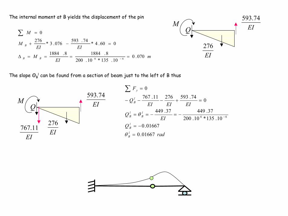
The internal moment at B yields the displacement of the pin

EI74.593

EI276

MQ

mEI

M

EIEIM

M

BB

B

070.010.135*10.200

8.18848.1884

060.4*74.593076.3*2760

66 ====∆

=−+

=

−

∑

The slope ΘBl can be found from a section of beam just to the left of B thus

rad

QEI

Q

EIEIEIQ

F

lB

lB

lB

lB

lB

y

01667.001667.0

10.135*10.20037.44937.449

074.59327611.767

0

66

=

−=

−=−==

=+−−−

=

−

∑

θ

θ

EI74.593

EI276

MQ

EI11.767

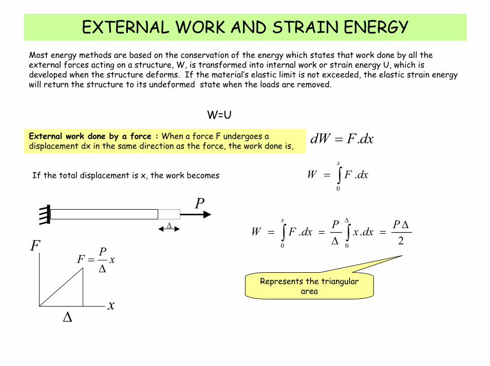
EXTERNAL WORK AND STRAIN ENERGYMost energy methods are based on the conservation of the energy which states that work done by all the external forces acting on a structure, W, is transformed into internal work or strain energy U, which is developed when the structure deforms. If the material’s elastic limit is not exceeded, the elastic strain energy will return the structure to its undeformed state when the loads are removed.

W=U

dxFdW .=External work done by a force : When a force F undergoes a displacement dx in the same direction as the force, the work done is,

∫=x

dxFW0

.If the total displacement is x, the work becomes

P∆

2..

00

∆=

∆== ∫∫

∆ PdxxPdxFWx

x

F

∆

xPF∆

=

Represents the triangular area

∆

x

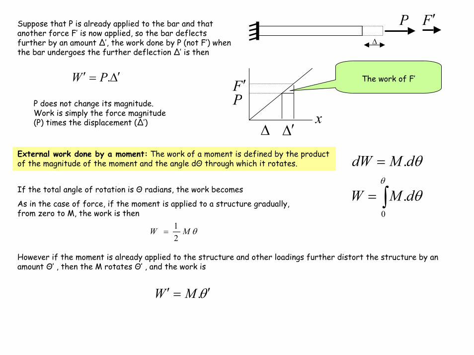
F ′

∆ ∆′

P

θ ′=′ .MW

P F ′Suppose that P is already applied to the bar and that another force F’ is now applied, so the bar deflects further by an amount ∆’, the work done by P (not F’) when the bar undergoes the further deflection ∆’ is then

∆′=′ .PW The work of F’

P does not change its magnitude. Work is simply the force magnitude (P) times the displacement (∆’)

External work done by a moment: The work of a moment is defined by the product of the magnitude of the moment and the angle dΘ through which it rotates.

∫=

=θ

θ

θ

0

.

.

dMW

dMdW

If the total angle of rotation is Θ radians, the work becomes

As in the case of force, if the moment is applied to a structure gradually, from zero to M, the work is then

θMW21

=

However if the moment is already applied to the structure and other loadings further distort the structure by an amount Θ’ , then the M rotates Θ’ , and the work is

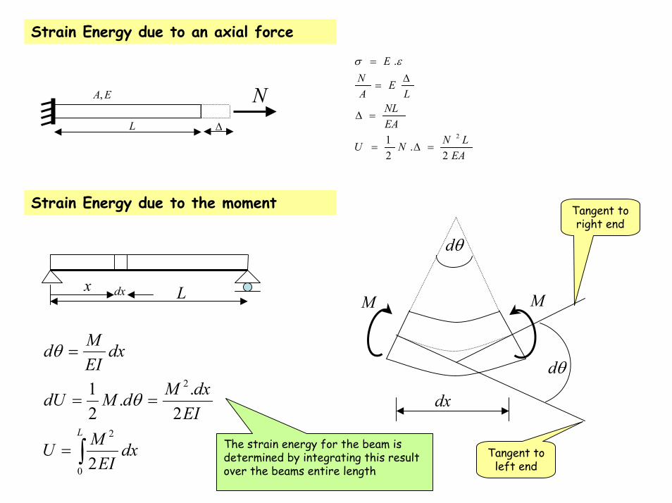
Strain Energy due to an axial force

EALNNU

EANL

LE

AN

E

2.

21

.

2

=∆=

=∆

∆=

= εσ

N∆L

EA,

Strain Energy due to the moment

θd

MM

θd

dx

Tangent to right end

x dx L

∫=

==

=

L

dxEIMU

EIdxMdMdU

dxEIMd

0

2

2

2

2..

21 θ

θ

The strain energy for the beam is determined by integrating this result over the beams entire length

Tangent to left end

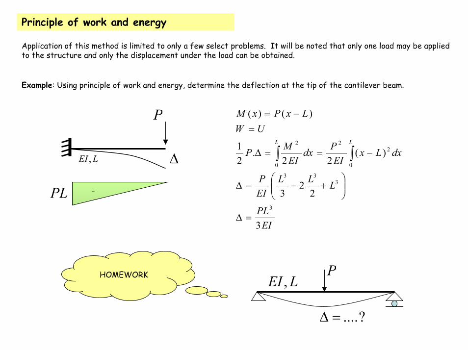
Principle of work and energy

Application of this method is limited to only a few select problems. It will be noted that only one load may be applied to the structure and only the displacement under the load can be obtained.

Example: Using principle of work and energy, determine the deflection at the tip of the cantilever beam.

P

EIPL

LLLEIP

dxLxEIPdx

EIMP

UWLxPxM

LL

3

22

3

)(22

.21

)()(

3

333

0

22

0

2

=∆

+−=∆

−==∆

=−=

∫∫LEI , ∆

-PL

P

?....=∆

LEI ,HOMEWORK

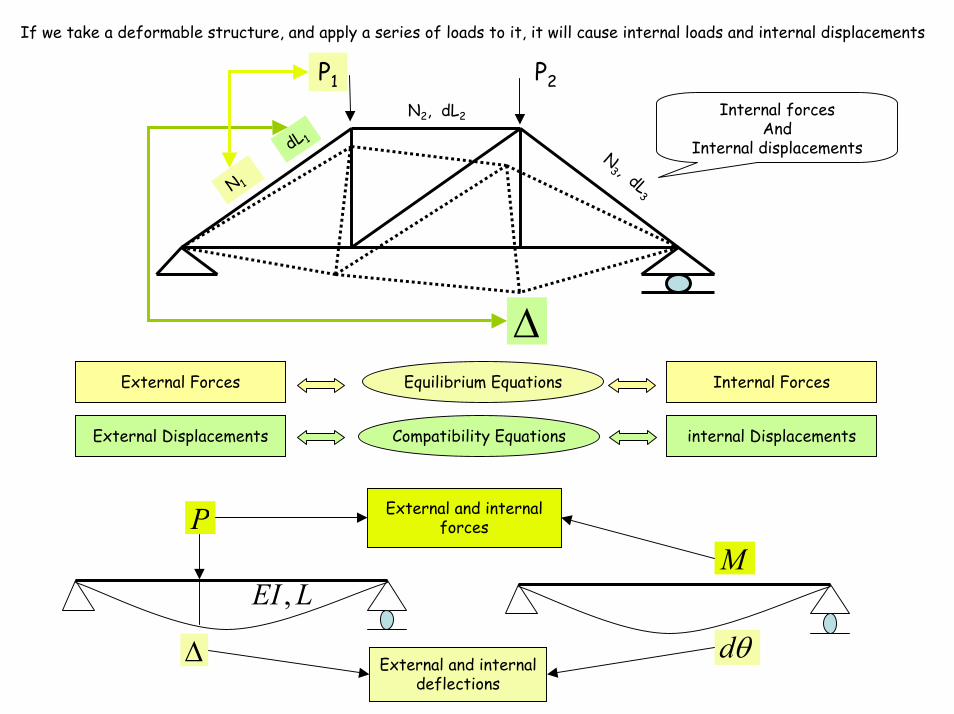
If we take a deformable structure, and apply a series of loads to it, it will cause internal loads and internal displacements

∆

N 1

N2, dL2

N3 , dL

3

dL 1

Internal forcesAnd

Internal displacements

P1 P2

Equilibrium Equations

Compatibility Equations

External Forces Internal Forces

External Displacements internal Displacements

P

LEI ,

∆

M

External and internalforces

θdExternal and internal

deflections

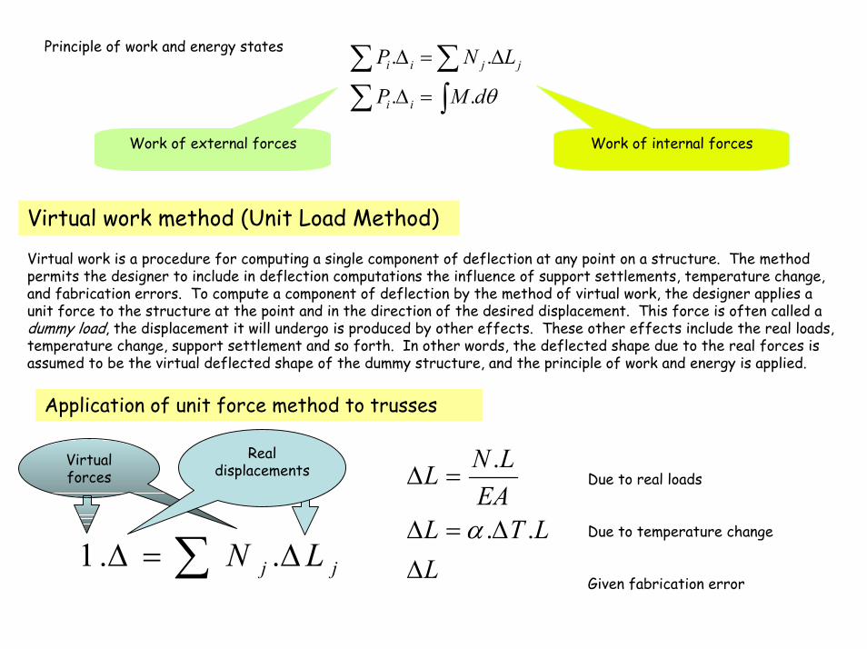
Principle of work and energy states

θdMP

LNP

ii

jjii

..

..

∫∑∑∑

=∆

∆=∆

Work of external forces Work of internal forces

Virtual work method (Unit Load Method)Virtual work is a procedure for computing a single component of deflection at any point on a structure. The method permits the designer to include in deflection computations the influence of support settlements, temperature change, and fabrication errors. To compute a component of deflection by the method of virtual work, the designer applies a unit force to the structure at the point and in the direction of the desired displacement. This force is often called a dummy load, the displacement it will undergo is produced by other effects. These other effects include the real loads, temperature change, support settlement and so forth. In other words, the deflected shape due to the real forces is assumed to be the virtual deflected shape of the dummy structure, and the principle of work and energy is applied.

Application of unit force method to trusses

jj LN ∆=∆ ∑ ..1

Real displacements

LLTL

EALNL

∆∆=∆

=∆

..

.

α

Virtual forces Due to real loads

Due to temperature change

Given fabrication error

A

B

C

kN225

m.4 m.4

5.62−

250−

5.37

5.187−200

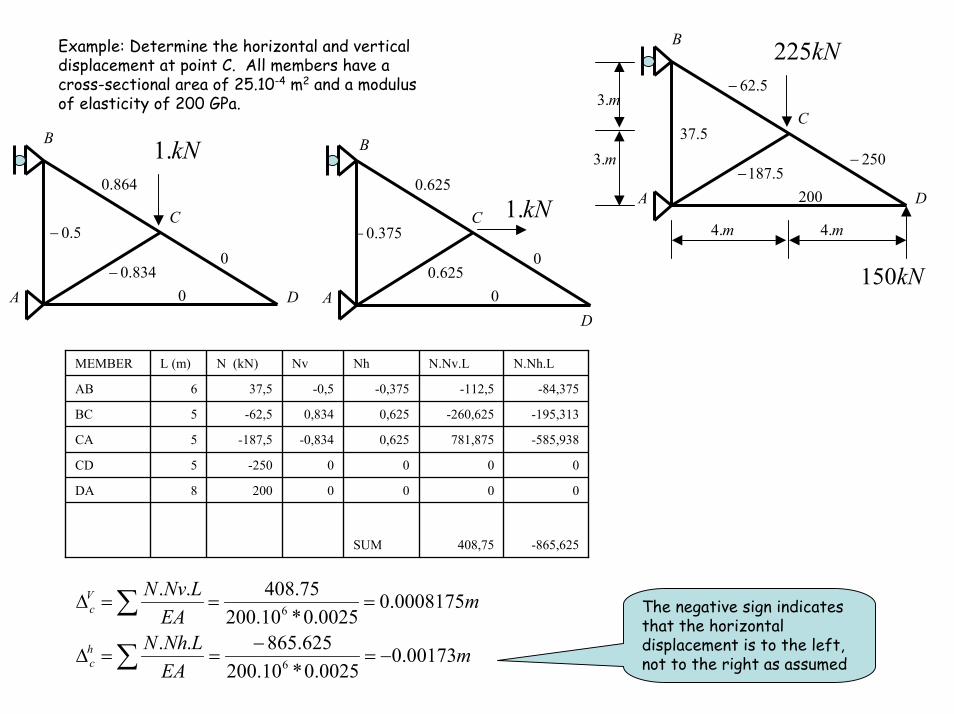
Example: Determine the horizontal and vertical displacement at point C. All members have a cross-sectional area of 25.10-4 m2 and a modulus of elasticity of 200 GPa.

m.3

A

C

D

kN.1625.0

0375.0−

625.00

B

m.3

A

B

C

kN.1864.0

05.0−

834.0−0

D

kN150D

-865,625408,75SUM

00002008DA

0000-2505CD

-585,938781,8750,625-0,834-187,55CA

-195,313-260,6250,6250,834-62,55BC

-84,375-112,5-0,375-0,537,56AB

N.Nh.LN.Nv.LNhNvN (kN)L (m)MEMBER

mEALNhN

mEALNvN

hc

Vc

00173.00025.0*10.200

625.865..

0008175.00025.0*10.200

75.408..

6

6

−=−

==∆

===∆

∑

∑ The negative sign indicates that the horizontal displacement is to the left, not to the right as assumed

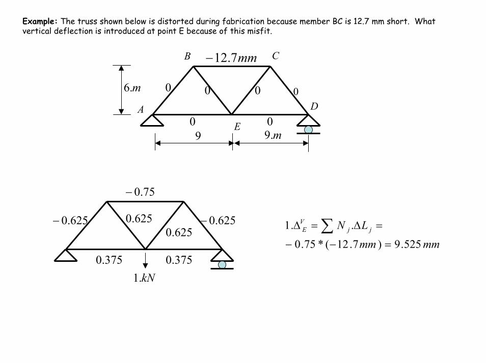
Example: The truss shown below is distorted during fabrication because member BC is 12.7 mm short. What vertical deflection is introduced at point E because of this misfit.

mm7.12−

D

CB

AE 0

000

0

0

m.99

m.6

75.0−

625.0−625.0− 625.0625.0

375.0375.0mmmm

LN jjVE

525.9)7.12(*75.0

..1

=−−

=∆=∆ ∑

kN.1

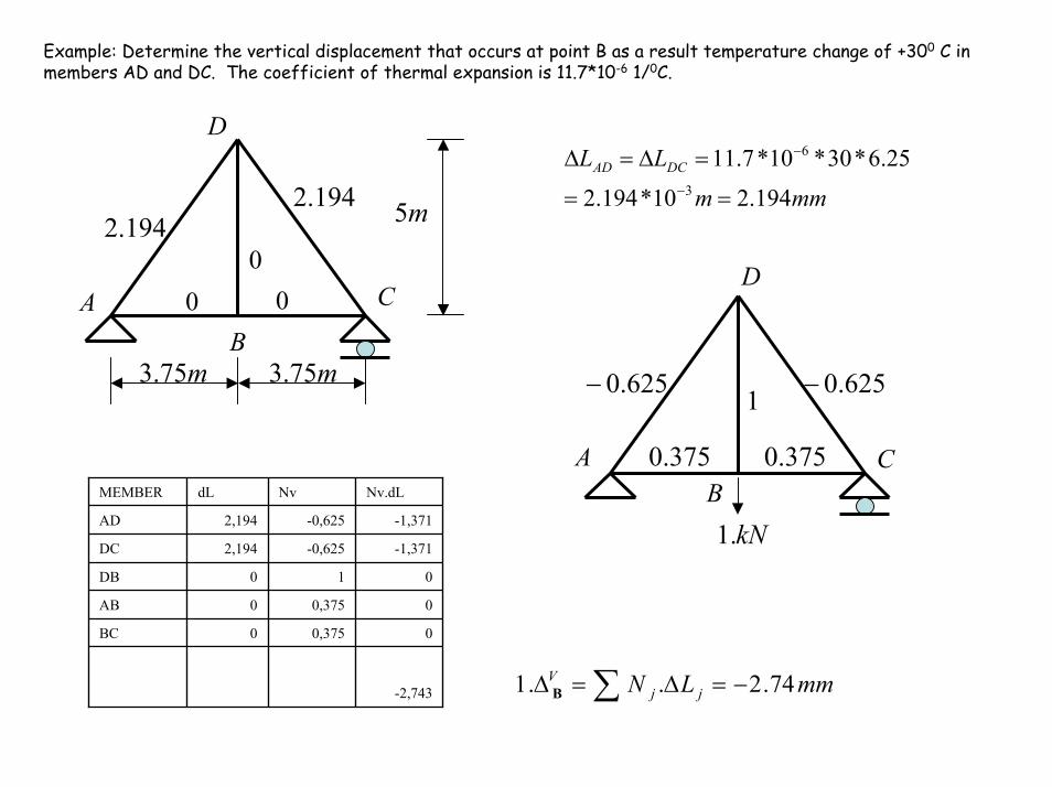
Example: Determine the vertical displacement that occurs at point B as a result temperature change of +300 C in members AD and DC. The coefficient of thermal expansion is 11.7*10-6 1/0C.

m75.3

m5

m75.3

194.2194.2

00 0

D

BA C

mmm

LL DCAD

194.210*194.2

25.6*30*10*7.113

6

==

=∆=∆−

−

D

625.0− 625.0−

375.0 375.0

1

A CB

-2,743

00,3750BC

00,3750AB

010DB

-1,371-0,6252,194DC

-1,371-0,6252,194AD

Nv.dLNvdLMEMBER

kN.1

mmLN jjV 74.2..1 −=∆=∆ ∑B

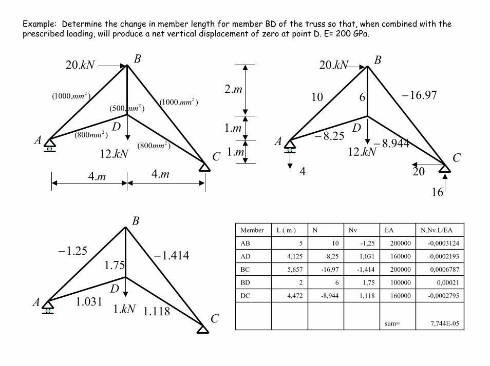
Example: Determine the change in member length for member BD of the truss so that, when combined with the prescribed loading, will produce a net vertical displacement of zero at point D. E= 200 GPa.

B

AC

D

m.4m.4

m.2

m.1

m.1

kN.20

kN.12

).1000( 2mm).1000( 2mm

)800( 2mm)800( 2mm

).500( 2mm

A

B

C

D

kN.12

kN.20

10 97.16−

944.8−25.8−

6

4 20

16

A

B

C

D

kN.1

414.1−

118.1031.1

25.1−75.1

7,744E-05sum=

-0,00027951600001,118-8,9444,472DC

0,000211000001,7562BD

0,0006787200000-1,414-16,975,657BC

-0,00021931600001,031-8,254,125AD

-0,0003124200000-1,25105AB

N.Nv.L/EAEANvNL ( m )Member

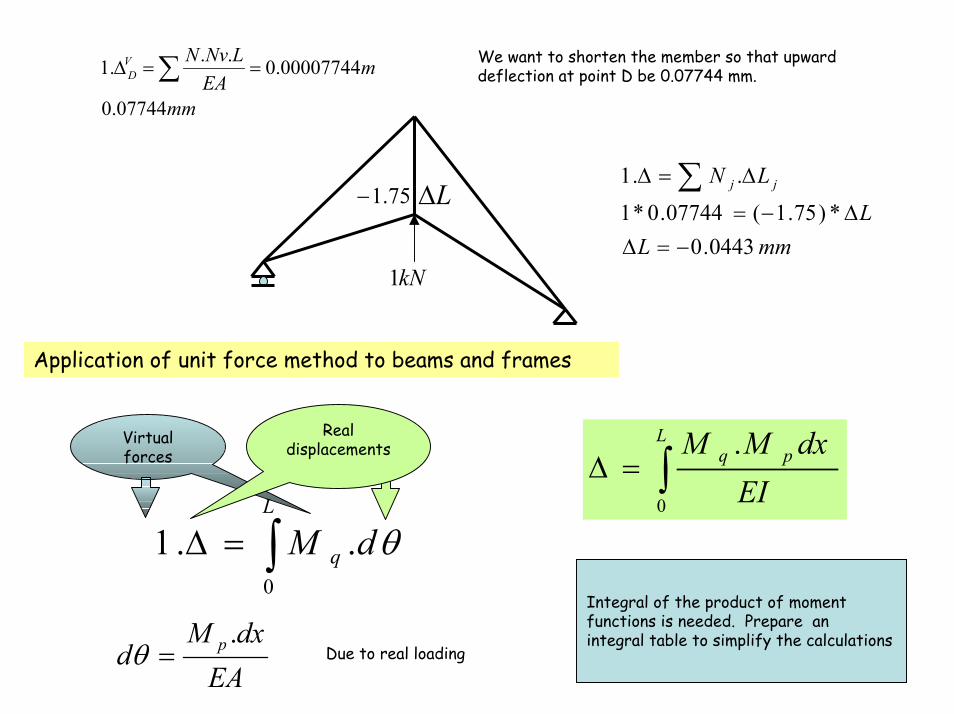
mm

mEALNvNV

D

07744.0

00007744.0...1 ==∆ ∑

kN1

75.1− L∆

We want to shorten the member so that upward deflection at point D be 0.07744 mm.

mmLL

LN jj

0443.0*)75.1(07744.0*1

..1

−=∆∆−=

∆=∆ ∑

Application of unit force method to beams and frames

θdML

q ..10∫=∆

Real displacements

∫=∆L

pq

EIdxMM

0

.Virtual forces

Integral of the product of moment functions is needed. Prepare an integral table to simplify the calculations

EAdxM

d p .=θ Due to real loading

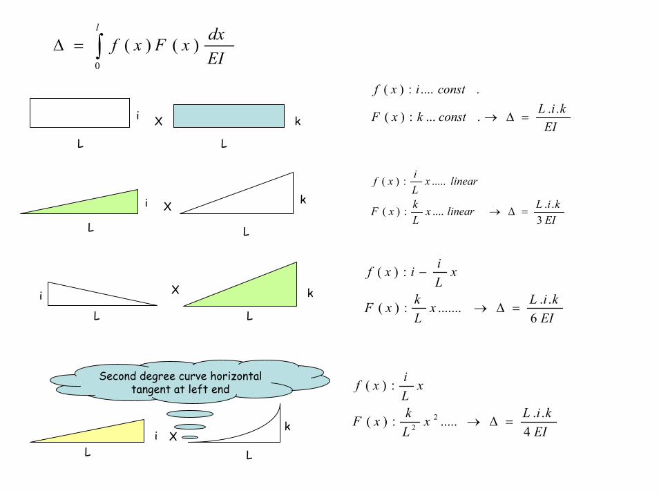
∫=∆l

EIdxxFxf

0

)()(

EIkiLconstkxF

constixf......:)(

.....:)(

=∆→

L L

i kX

EIkiLlinearx

LkxF

linearxLixf

3......:)(

.....:)(

=∆→i k

LL

X

EIkiLx

LkxF

xLiixf

6.........:)(

:)(

=∆→

−

L L

i kX

k

Second degree curve horizontal tangent at left end

EIkiLx

LkxF

xLixf

4.......:)(

:)(

22 =∆→

i XL L

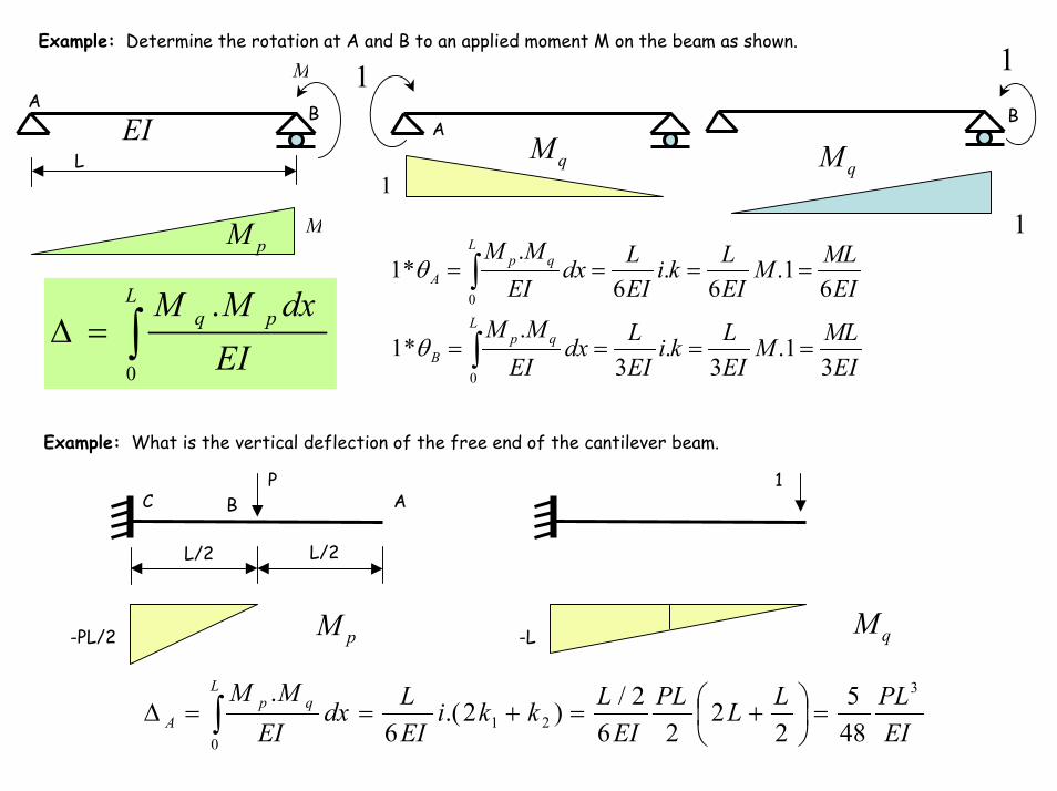
Example: Determine the rotation at A and B to an applied moment M on the beam as shown.

AqM qM

1 1

1

1

B

EIMLM

EILki

EILdx

EIMML qp

A 61.

6.

6.

*10

==== ∫θ

EIMLM

EILki

EILdx

EIMML qp

B 31.

3.

3.

*10

==== ∫θ

M

BEIL

A

pM M

∫=∆L

pq

EIdxMM

0

.

Example: What is the vertical deflection of the free end of the cantilever beam.

BCP 1

A

L/2L/2

qMpM -L-PL/2

EIPLLLPL

EILkki

EILdx

EIMML qp

A

3

210 48

52

226

2/)2.(6

.=

+=+==∆ ∫

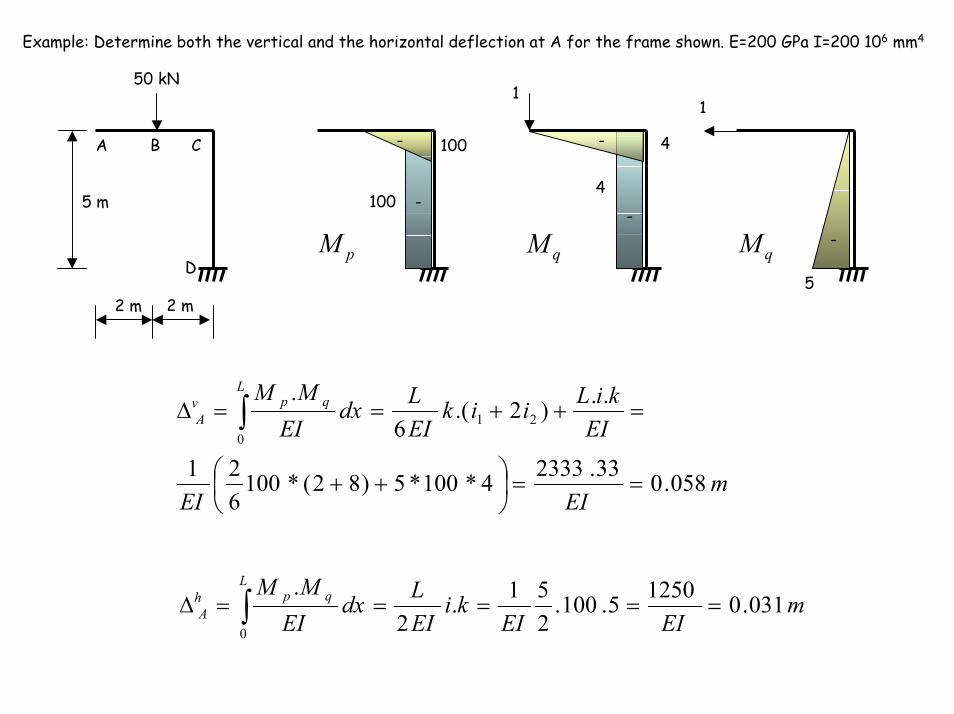
Example: Determine both the vertical and the horizontal deflection at A for the frame shown. E=200 GPa I=200 106 mm4

50 kN

5 m

A B C

DqM

4

4-

-

11

qM5

-pM

100

100

-

-

2 m2 m

mEIEI

EIkiLiik

EILdx

EIMML qpv

A

058.033.23334*100*5)82(*100621

..)2.(6

.21

0

==

++

=++==∆ ∫

mEIEI

kiEILdx

EIMML qph

A 031.012505.100.251.

2.

0

=====∆ ∫

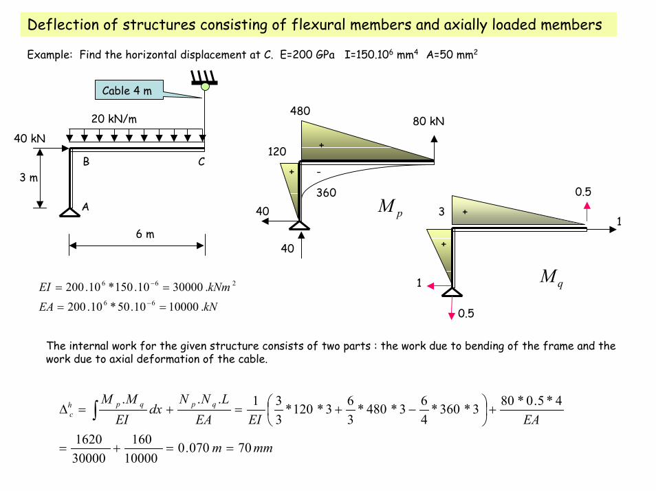
Deflection of structures consisting of flexural members and axially loaded members

Example: Find the horizontal displacement at C. E=200 GPa I=150.106 mm4 A=50 mm2

Cable 4 m

A

B C

80 kN480

360

120 +

-+

pM40

0.5

1 qM

+

+

20 kN/m

40 kN

3 m

3

6 m1

40

kNEAkNmEI

.1000010.50*10.200.3000010.150*10.200

66

266

==

==−

−

0.5

The internal work for the given structure consists of two parts : the work due to bending of the frame and the work due to axial deformation of the cable.

mmm

EAEIEALNN

dxEIMM qpqph

c

70070.010000

160300001620

4*5.0*803*360*463*480*

363*120*

331...

==+=

+

−+=+=∆ ∫

10 kN/m

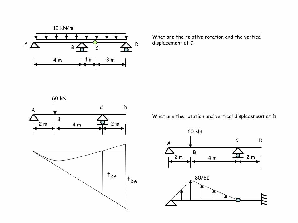
What are the relative rotation and the vertical displacement at C

B CA D

1 m 3 m4 m

60 kN

DCAWhat are the rotation and vertical displacement at DB

2 m2 m 4 m60 kN

tCA tDA

DCA

B2 m2 m 4 m

80/EI

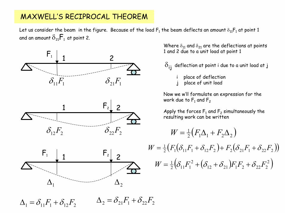
MAXWELL’S RECIPROCAL THEOREMLet us consider the beam in the figure. Because of the load F1 the beam deflects an amount δ11F1 at point 1 and an amount δ21F1 at point 2.

Where δ11 and δ21 are the deflections at points 1 and 2 due to a unit load at point 1

δij deflection at point i due to a unit load at j

i place of deflection j place of unit load

Now we w’ll formulate an expression for the work due to F1 and F2

Apply the forces F1 and F2 simultaneously the resulting work can be written

F1

111Fδ 121Fδ

21

212Fδ 222Fδ

F21 2

( )221121 ∆+∆= FFW

( ) ( )( )2221212212111121 FFFFFFW δδδδ +++=

F1 F2

1∆ 2∆

1 2( )( )2

2222121122

11121 FFFFW δδδδ +++=

2221212 FF δδ +=∆2121111 FF δδ +=∆

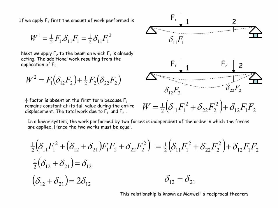
F1If we apply F1 first the amount of work performed is

111Fδ

21

21112

111112

11 . FFFW δδ ==

Next we apply F2 to the beam on which F1 is already acting. The additional work resulting from the application of F2 F1 F2

222Fδ212Fδ

21( ) ( )22222

12121

2 FFFFW δδ +=

( ) 21122

2222

11121 FFFFW δδδ ++=

½ factor is absent on the first term because F1remains constant at its full value during the entire displacement. The total work due to F1 and F2 .

In a linear system, the work performed by two forces is independent of the order in which the forces are applied. Hence the two works must be equal.

( ) 21122

2222

11121 FFFF δδδ ++=( )( )2

2222121122

11121 FFFF δδδδ +++

( ) 12211221 δδδ =+

( ) 122112 2δδδ =+ 2112 δδ =This relationship is known as Maxwell’ s reciprocal theorem

1 1

21δ 12δ

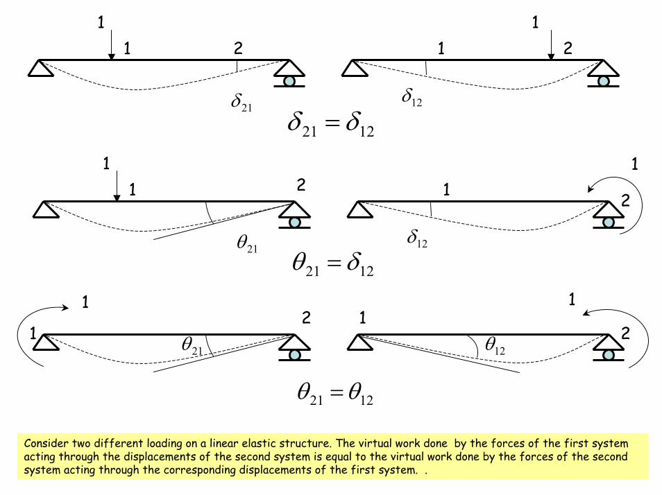
1221 δδ =

2 21 1

21θ 12δ

2

1221 δθ =

1 121 1

21θ112θ 2

1221 θθ =

112 1

Consider two different loading on a linear elastic structure. The virtual work done by the forces of the first system acting through the displacements of the second system is equal to the virtual work done by the forces of the second system acting through the corresponding displacements of the first system. .

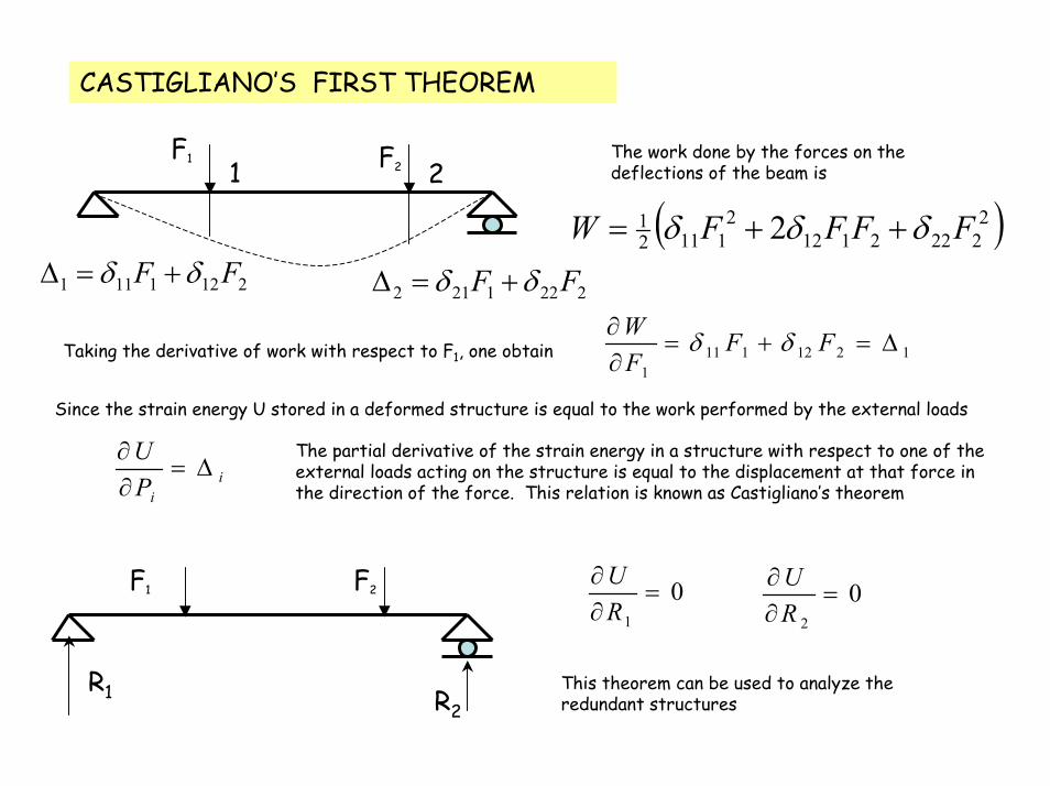
CASTIGLIANO’S FIRST THEOREM

F1 F2The work done by the forces on the deflections of the beam is

( )22222112

21112

1 2 FFFFW δδδ ++=2121111 FF δδ +=∆

2221212 FF δδ +=∆

1 2

12121111

∆=+=∂∂ FFFW δδTaking the derivative of work with respect to F1, one obtain

Since the strain energy U stored in a deformed structure is equal to the work performed by the external loads

iiPU

∆=∂∂ The partial derivative of the strain energy in a structure with respect to one of the

external loads acting on the structure is equal to the displacement at that force in the direction of the force. This relation is known as Castigliano’s theorem

01

=∂∂RUF1 F2 0

2

=∂∂RU

R1 This theorem can be used to analyze the redundant structures R2

F2F1

0=∂∂RU

R

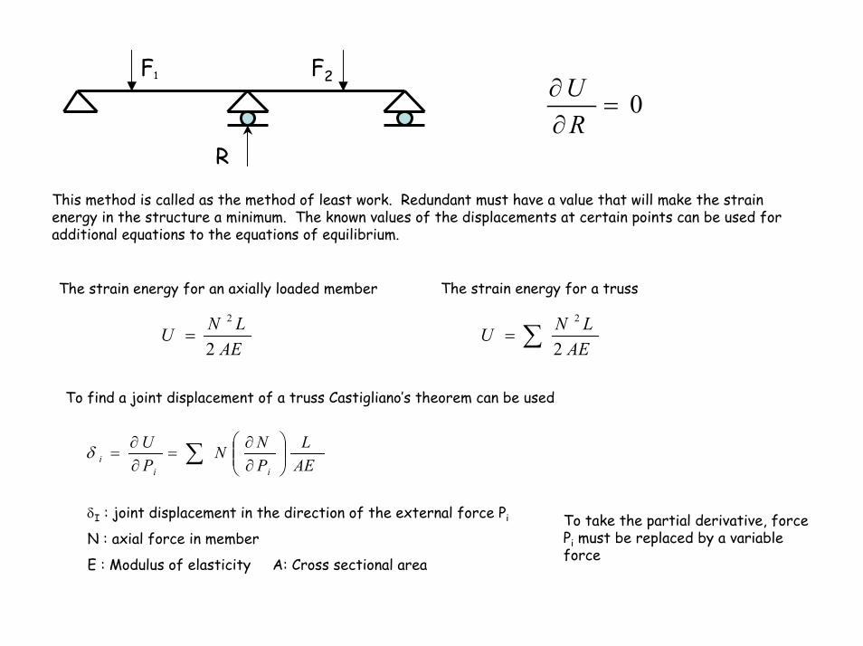
This method is called as the method of least work. Redundant must have a value that will make the strain energy in the structure a minimum. The known values of the displacements at certain points can be used for additional equations to the equations of equilibrium.

The strain energy for a trussThe strain energy for an axially loaded member

AELNU

2

2

= ∑=AELNU

2

2

To find a joint displacement of a truss Castigliano’s theorem can be used

AEL

PNN

PU

iii ∑

∂∂

=∂∂

=δ

δI : joint displacement in the direction of the external force Pi

N : axial force in member

E : Modulus of elasticity A: Cross sectional area

To take the partial derivative, force Pi must be replaced by a variable force

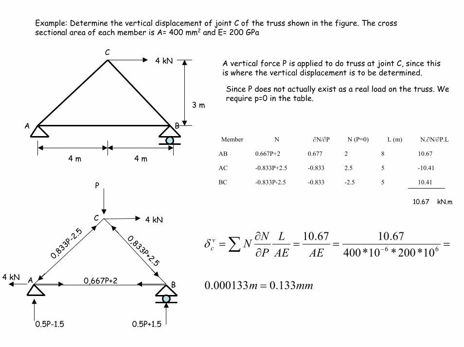
Example: Determine the vertical displacement of joint C of the truss shown in the figure. The cross sectional area of each member is A= 400 mm2 and E= 200 GPa

4 kN

A B

CA vertical force P is applied to do truss at joint C, since thisis where the vertical displacement is to be determined.

Since P does not actually exist as a real load on the truss. We require p=0 in the table.

3 m

10.415-2.5-0.833-0.833P-2.5BC

-10.4152.5-0.833-0.833P+2.5AC

10.67820.6770.667P+2AB

N.∂Ν/∂P.LL (m)N (P=0)∂Ν/∂PNMember

4 m 4 m

P

10.67 kN.m

A B

C

0,833

P-2.5 0,833P+2.5

0,667P+24 kN

0.5P-1.5

4 kN

mmm

AEAEL

PNNv

c

133.0000133.0

10*200*10*40067.1067.10

66

=

===∂∂

= −∑δ

0.5P+1.5

6.667+0.667P

6.667+0.667P13.333+0.333P

-(18.85

6+0.47

1P)

13.3

33+0

.333

P

-(13.333+0.333P)

P9.429

-0.47

1P-(9.429+0.943P)

(13.333+0.333P)(6.667+0.667P)

AB C D

F E

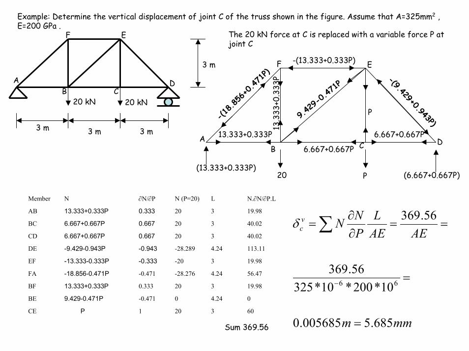
Example: Determine the vertical displacement of joint C of the truss shown in the figure. Assume that A=325mm2 , E=200 GPa .

EF

3 m 3 m

20 kN 20 kN

AB C

D

3 m

3 m

The 20 kN force at C is replaced with a variable force P at joint C

20 P

603201PCE

04.240-0.4719.429-0.471PBE

19.983200.33313.333+0.333PBF

56.474.24-28.276-0.471-18.856-0.471PFA

19.983-20-0.333-13.333-0.333PEF

113.114.24-28.289-0.943-9.429-0.943PDE

40.023200.6676.667+0.667PCD

40.023200.6676.667+0.667PBC

19.983200.33313.333+0.333PAB

N.∂N/∂P.LLN (P=20)∂N/∂PNMember

mmm

AEAEL

PNNv

c

685.5005685.0

10*200*10*32556.369

56.369

66

=

=

==∂∂

=

−

∑δ

Sum 369.56

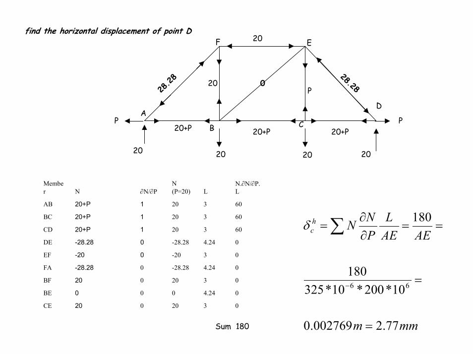
28.28 20

P0

28.28

AC

D

F E

20+P

find the horizontal displacement of point D20

P PB20+P 20+P

20 20 2020

0320020CE

04.24000BE

0320020BF

04.24-28.280-28.28FA

03-200-20EF

04.24-28.280-28.28DE

60320120+PCD

60320120+PBC

60320120+PAB

N.∂N/∂P.LL

N (P=20)∂N/∂PN

Member

mmm

AEAEL

PNNh

c

77.2002769.0

10*200*10*325180

180

66

=

=

==∂∂

=

−

∑δ

Sum 180

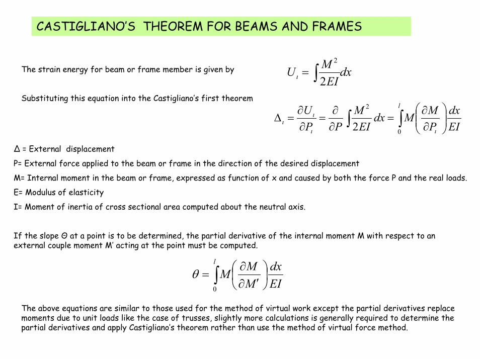
CASTIGLIANO’S THEOREM FOR BEAMS AND FRAMES

dxEIMU ı ∫= 2

2The strain energy for beam or frame member is given by

Substituting this equation into the Castigliano’s first theorem

∫ ∫

∂∂

=∂∂

=∂∂

=∆l

ıı

ıı EI

dxPMMdx

EIM

PPU

0

2

2

∆ = External displacement

P= External force applied to the beam or frame in the direction of the desired displacement

M= Internal moment in the beam or frame, expressed as function of x and caused by both the force P and the real loads.

E= Modulus of elasticity

I= Moment of inertia of cross sectional area computed about the neutral axis.

If the slope Θ at a point is to be determined, the partial derivative of the internal moment M with respect to an external couple moment M’ acting at the point must be computed.

EIdx

MMM

l

∫

′∂∂

=0

θ

The above equations are similar to those used for the method of virtual work except the partial derivatives replace moments due to unit loads like the case of trusses, slightly more calculations is generally required to determine the partial derivatives and apply Castigliano’s theorem rather than use the method of virtual force method.

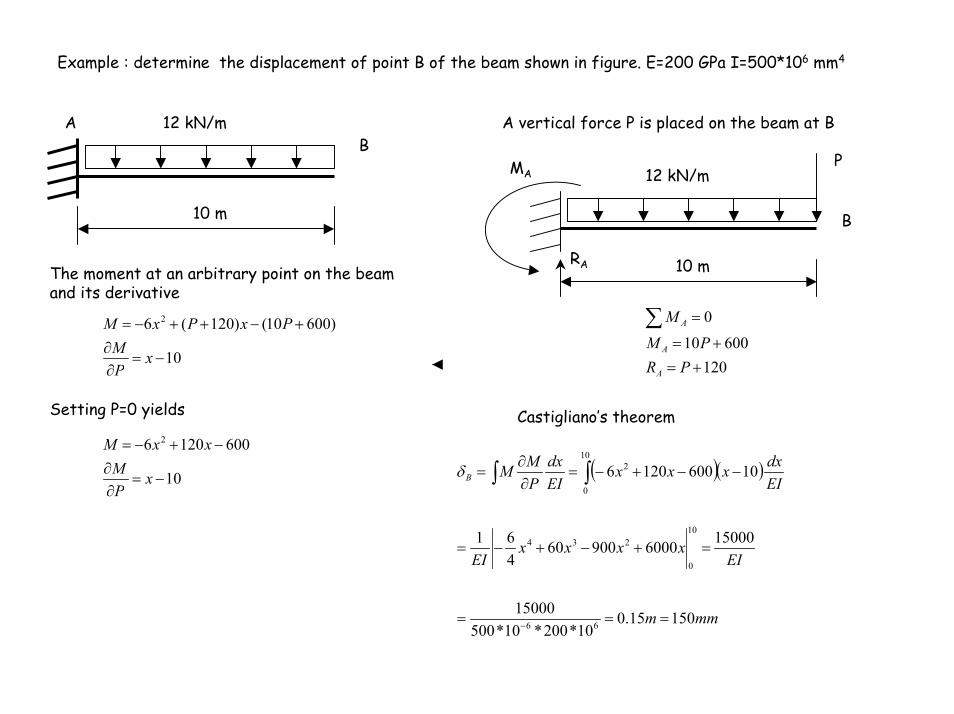
Example : determine the displacement of point B of the beam shown in figure. E=200 GPa I=500*106 mm4

A vertical force P is placed on the beam at BA 12 kN/mB

P

10 m

MA

RA

12 kN/m

B

10 mThe moment at an arbitrary point on the beam and its derivative

12060010

0

+=+=

=∑

PRPM

M

A

A

A

10

)60010()120(6 2

−=∂∂

+−++−=

xPM

PxPxM

Setting P=0 yields Castigliano’s theorem

10

6001206 2

−=∂∂

−+−=

xPM

xxM

( )( )

mmm

EIxxxx

EI

EIdxxxx

EIdx

PMMB

15015.010*200*10*500

15000

15000600090060461

106001206

66

10

0

234

10

0

2

===

=+−+−=

−−+−=∂∂

=

−

∫∫δ

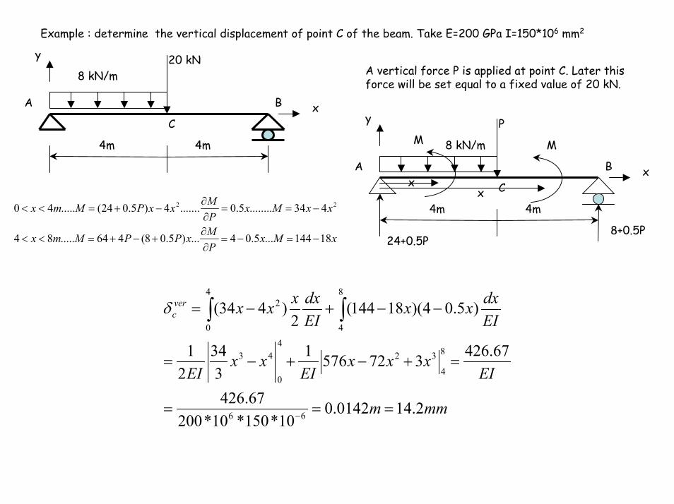
Example : determine the vertical displacement of point C of the beam. Take E=200 GPa I=150*106 mm2

y 20 kNA vertical force P is applied at point C. Later this force will be set equal to a fixed value of 20 kN.

8 kN/m

A B xyC

4m 4m

PM M8 kN/m

4m 4m

A B

Cx

xx

xMxPMxPPMmx

xxMxPMxxPMmx

18144...5.04...)5.08(464.....84

434........5.0.......4)5.024(.....40 22

−=−=∂∂

+−+=<<

−==∂∂

−+=<<

8+0.5P24+0.5P

mmm

EIxxx

EIxx

EI

EIdxxx

EIdxxxxver

c

2.140142.010*150*10*200

67.426

67.42637257613

342

1

)5.04)(18144(2

)434(

66

8

4

324

0

43

8

4

4

0

2

===

=+−+−=

−−+−=

−

∫∫δ

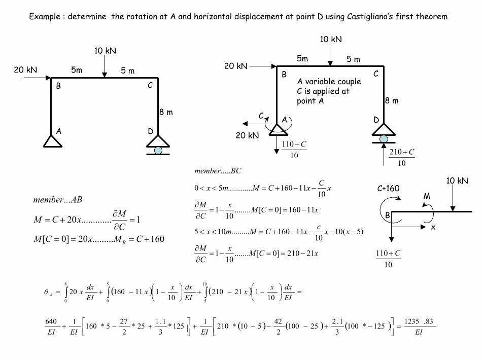
Example : determine the rotation at A and horizontal displacement at point D using Castigliano’s first theorem

D

8 m

10 kN

A

5m

CB

5 m20 kNA variable couple C is applied at point A

10 kN

5m 5 m20 kN

CB

D

8 m

AC

20 kN

10110 C+

10210 C+

xCMxCM

xxcxCMmx

xCMxCM

xCxCMmx

BCmember

21210]0[.......10

1

)5(1010

11160.........105

11160]0[........10

1

1011160............50

.....

−==−=∂∂

−−−−+=<<

−==−=∂∂

−−+=<<

160.........20]0[

1.............20

...

+===

=∂∂

+=

CMxCMCMxCM

ABmember

B

( ) ( )

( ) ( ) ( )EIEIEIEI

EIdxxx

EIdxxx

EIdxxA

83.1235125*1003

1.2251002

42510*2101125*31.125*

2275*1601640

10121210

1011116020

10

5

8

0

5

0

=

−+−−−+

+−+

=

−−+

−−+= ∫∫ ∫θ

10 kN

x

C+160M

B

10110 C+

Example : determine the reactions for the propped cantilever beam.A P

B

M P M

L/2 L/2

MA

AB

xx

C

R

Reaction at point C is taken as redundant

MA=PL/2-RLP-R

PR

EIdxxLxLR

EIdxxLRLPLxRP

EIdx

RMM

RU

xLRMxLRMLxL

xLRMRLPLxRPMLx

L

L

L

L

165

0))(()()2

)((

0

..................).........(.....2

.........2

)(.....2

0

2

2

0

0

=

=−−+−+−−

=∂∂

=∂∂

−=∂∂

−=<<

−=∂∂

+−−=<<

∫∫

∫

Homework, Take the moment at A as redundant force

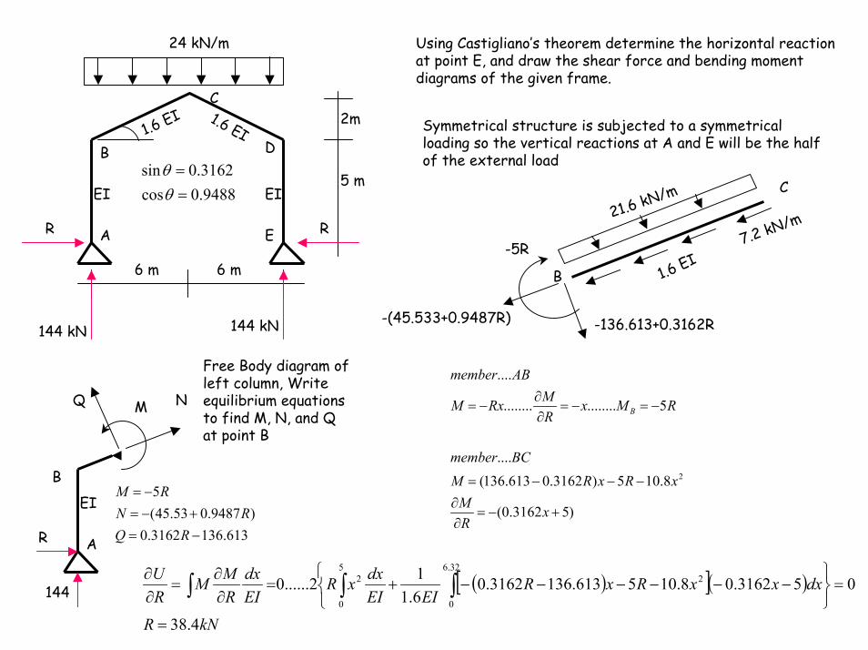
24 kN/m Using Castigliano’s theorem determine the horizontal reaction at point E, and draw the shear force and bending moment diagrams of the given frame.

A

D

C

B

E

EIEI

1.6 EI1.6 EI

9488.0cos3162.0sin

==

θθ

2m

5 m

Symmetrical structure is subjected to a symmetrical loading so the vertical reactions at A and E will be the half of the external load

21.6 kN/m

7.2 kN/m

B

C

1.6 EI

R R-5R

6 m 6 m

-(45.533+0.9487R) -136.613+0.3162R144 kN144 kN

)53162.0(

8.105)3162.0613.136(....

5................

....

2

+−=∂∂

−−−=

−=−=∂∂

−=

xRM

xRxRMBCmember

RMxRMRxM

ABmember

B

A

EI

613.1363162.0)9487.053.45(

5

−=+−=

−=

RQRN

RM

( )[ ]( )

kNR

dxxxRxREIEI

dxxREIdx

RMM

RU

4.38

053162.08.105613.1363162.06.112......0

5

0

32.6

0

22

=

=

−−−−−−+=∂∂

=∂∂

∫ ∫∫

Free Body diagram of left column, Write equilibrium equations to find M, N, and Q at point B

NQ M

B

R

144

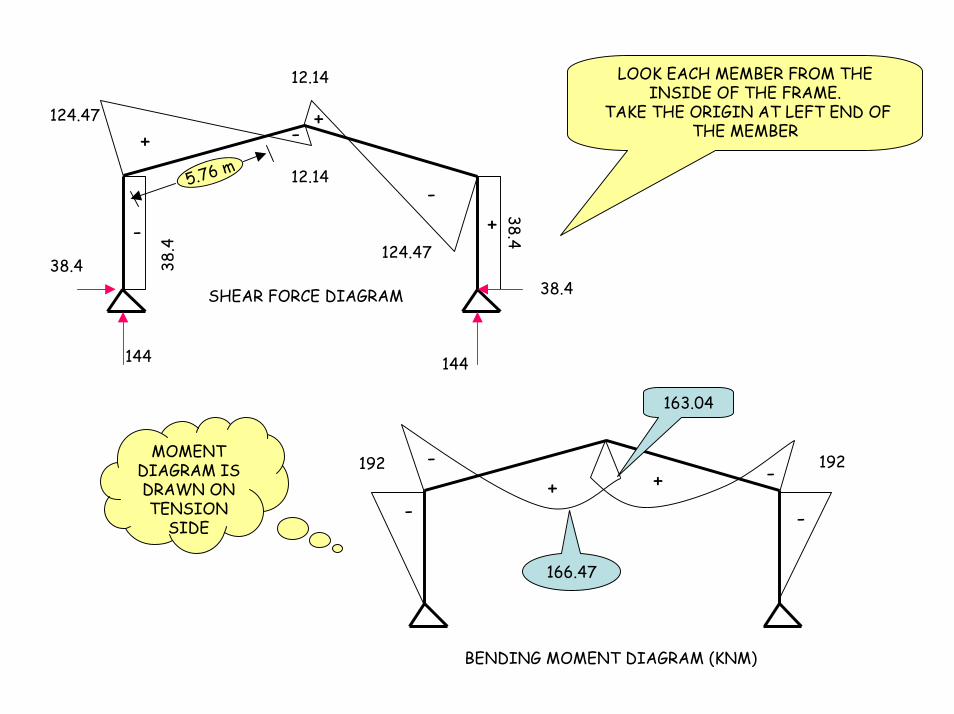
LOOK EACH MEMBER FROM THE INSIDE OF THE FRAME.

TAKE THE ORIGIN AT LEFT END OF THE MEMBER

12.14

124.47

124.47

12.1438

.4

38.4

++

+-

-

-

144

5.76 m

38.438.4SHEAR FORCE DIAGRAM

144

-

++ --

-

163.04

MOMENT DIAGRAM IS DRAWN ON TENSION

SIDE

192192

166.47

BENDING MOMENT DIAGRAM (KNM)