maximum likelihood estimation - department of political ... - cunha.pdf · introductory maximum...
TRANSCRIPT

Maximum Likelihood EstimationAdditional Topics
Raphael Cunha
Program in Statistics and Methodology – PRISM
Department of Political Science
The Ohio State University
March 28, 2014

Overview
We will cover two topics that are not usually covered inintroductory maximum likelihood estimation (MLE) courses:
• Interpretation of multiplicative interaction terms in nonlinearmodels
• Models for truncation and sample selection (Tobit and theHeckman selection model)

Interaction terms in nonlinear models

Interaction terms in linear models (recap)
• We often have conditional hypotheses that can be captured bymultiplicative interaction models. E.g.:
H1: An increase in X is associated with an increase in Y whencondition Z is met, but not when condition Z is absent.
• Suppose that Y and X are continuous and Z is dichotomous.We can write a simple linear interactive model:
Y = β0 + β1X + β2Z + β3XZ + ε
• The marginal effect of X on Y (the effect of a one-unit changein X on Y) is given by:
∂Y∂X = β1 + β3Z
• When Z = 0, ∂Y∂X = β1. When Z = 1, ∂Y
∂X = β1 + β3.

Interaction terms in linear models
Figure: Brambor et al. 2006

Interaction terms in linear models
• We’re usually not interested in the statistical significance orinsignificance of the model parameters themselves. We careabout ∂Y
∂X , so we want to know the standard error of thisquantity, which is given by:
σ̂ ∂Y∂X
=√
var(β̂1) + Z 2var(β̂3) + 2Zcov(β̂1β̂3)
• If Z is dichotomous, we need only compute s.e.’s for ∂Y∂X for
when Z = 0 and Z = 1.
• If Z is continuous, useful to plot ∂Y∂X against a substantively
meaningful range of Z, using same formula above for the 95%confidence intervals

Interaction terms in linear models
Figure: Marginal effect of temporally proximate presidential elections on the effectivenumber of electoral parties. Example from Brambor et al. 2006.

Interaction terms in nonlinear models
• What about nonlinear models?
• Some have argued that it’s not necessary to include aninteraction term, because models like logit and probit forceeffect of all independent variables to depend on each other.E.g., consider the probit model:
E [Y ] = Φ(β0 + β1X + β2Z ) = Φ(·)
• Marginal effect of X is: ∂Φ(·)∂X = β1Φ′(·)
• Marginal effect of X depends on other independent variableswhether the hypothesis being tested is conditional or not. It’sjust a function of how the model is parameterized. Tosubstantively test a conditional hypothesis, one must includean interaction term, just like in the linear case (see Bramboret al. 2006)

Interaction terms in nonlinear models
• Ai & Norton 2003 show that interpreting interaction effects innonlinear models is a lot more complicated than in linear ones
• For example, in our previous linear interactive model with acontinuous Y, interaction effect of X and Z is cross-derivativeof E[Y]:
∂2E [Y |X ,Z ]∂X∂Z = β3
(But remember that not much can be learned from thestatistical significance of β3 alone)

Interaction terms in nonlinear models
• However, intuition does not extend to nonlinear models.Consider a dichotomous y , two independent variables ofinterest, x and z , and a vector of additional independentvariables W. A simple interactive probit model:
E [y |x , z ,W] = Φ(β1x + β2z + β3xz + Wβ) = Φ(·)
• The interaction effect of x and z is the cross-derivative of theexpected value of y :
∂2Φ(·)∂x∂z = β3Φ′(·) + (β1 + β3z)(β2 + β3x)Φ′′(·)
• Very hard to interpret!
Interaction terms in nonlinear models
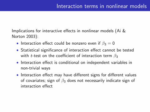
Implications for interactive effects in nonlinear models (Ai &Norton 2003):
• Interaction effect could be nonzero even if β3 = 0
• Statistical significance of interaction effect cannot be testedwith t-test on the coefficient of interaction term β3
• Interaction effect is conditional on independent variables innon-trivial ways
• Interaction effect may have different signs for different valuesof covariates; sign of β3 does not necessarily indicate sign ofinteraction effect
Interaction terms in nonlinear models
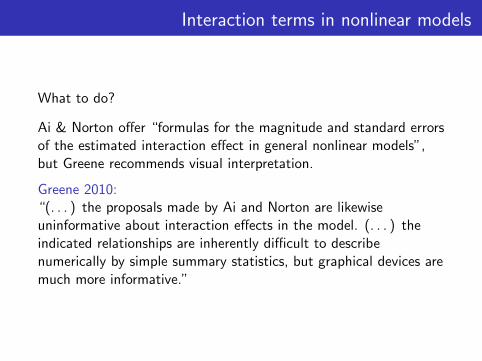
What to do?
Ai & Norton offer “formulas for the magnitude and standard errorsof the estimated interaction effect in general nonlinear models”,but Greene recommends visual interpretation.
Greene 2010:“(. . . ) the proposals made by Ai and Norton are likewiseuninformative about interaction effects in the model. (. . . ) theindicated relationships are inherently difficult to describenumerically by simple summary statistics, but graphical devices aremuch more informative.”
Example
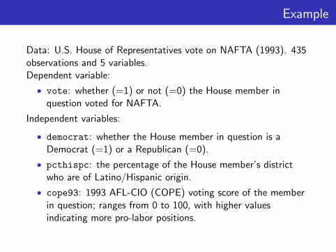
Data: U.S. House of Representatives vote on NAFTA (1993). 435observations and 5 variables.Dependent variable:
• vote: whether (=1) or not (=0) the House member inquestion voted for NAFTA.
Independent variables:
• democrat: whether the House member in question is aDemocrat (=1) or a Republican (=0).
• pcthispc: the percentage of the House member’s districtwho are of Latino/Hispanic origin.
• cope93: 1993 AFL-CIO (COPE) voting score of the memberin question; ranges from 0 to 100, with higher valuesindicating more pro-labor positions.

Example
We have the following hypotheses:
• Higher COPE scores will correspond to lower probabilities ofvoting for NAFTA
• The effect of the former will be moderated by political party.In particular, the (negative) effect of COPE scores onpro-NAFTA voting will be greater for Democrats than forRepublicans.
So we estimate an interactive logit model:
Pr(Y = 1|X ) =Λ(β0+β1democrat+β2cope93+β3democrat∗cope93+β4pcthispc),
where Λ is the logistic CDF.

Example
Figure: Logit parameter estimates for the probability of voting for NAFTA.

Example
0.25
0.50
0.75
1.00
0 25 50 75 100Pro−labor score
Pre
dict
ed p
roba
bilit
y of
vot
ing
for
NAT
A
Figure: Predicted probability of voting for NAFTA as a function of pro-labor score(COPE93) for Democrats (continuous line) and Republicans (dashed line). Shadedareas are 95% bootstrapped CIs.

Example
−0.8
−0.7
−0.6
−0.5
Republican Democrat
Pre
dict
ed c
hang
e in
pro
babi
lity
of v
otin
g fo
r N
ATA
Figure: Discrete change in predicted probability of voting for NAFTA from amean-centered, 2-standard-deviation change in COPE93 for Democrats andRepublicans. Vertical bars are 95% bootstrapped CIs.

Example
Software implementation:
• Example R code available with the accompanying presentationmaterials
• Stata users: Be careful when using multiplicative interactionsin Stata. The most common way of creating interaction termsis to generate a new variable equal to the product of the twointeracting variables. If you do this, Stata will treat theinteraction term as a third, distinct variable rather than twovariables being interacted. When computing predictedprobabilities, you might get wrong results. Make sure youknow what the functions you are using are doing.
Interaction terms in nonlinear models
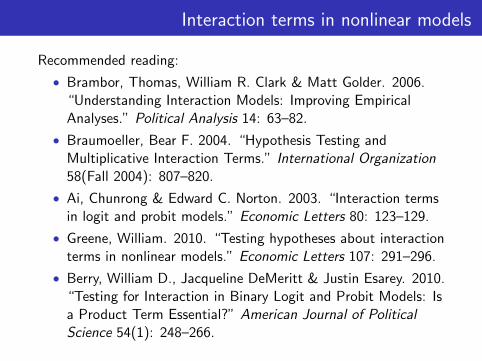
Recommended reading:
• Brambor, Thomas, William R. Clark & Matt Golder. 2006.“Understanding Interaction Models: Improving EmpiricalAnalyses.” Political Analysis 14: 63–82.
• Braumoeller, Bear F. 2004. “Hypothesis Testing andMultiplicative Interaction Terms.” International Organization58(Fall 2004): 807–820.
• Ai, Chunrong & Edward C. Norton. 2003. “Interaction termsin logit and probit models.” Economic Letters 80: 123–129.
• Greene, William. 2010. “Testing hypotheses about interactionterms in nonlinear models.” Economic Letters 107: 291–296.
• Berry, William D., Jacqueline DeMeritt & Justin Esarey. 2010.“Testing for Interaction in Binary Logit and Probit Models: Isa Product Term Essential?” American Journal of PoliticalScience 54(1): 248–266.
Models for sample selection
Censoring and truncation
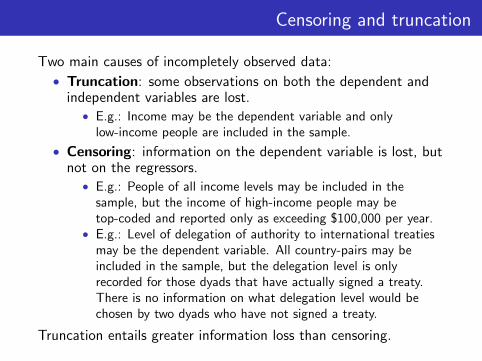
Two main causes of incompletely observed data:
• Truncation: some observations on both the dependent andindependent variables are lost.
• E.g.: Income may be the dependent variable and onlylow-income people are included in the sample.
• Censoring: information on the dependent variable is lost, butnot on the regressors.
• E.g.: People of all income levels may be included in thesample, but the income of high-income people may betop-coded and reported only as exceeding $100,000 per year.
• E.g.: Level of delegation of authority to international treatiesmay be the dependent variable. All country-pairs may beincluded in the sample, but the delegation level is onlyrecorded for those dyads that have actually signed a treaty.There is no information on what delegation level would bechosen by two dyads who have not signed a treaty.
Truncation entails greater information loss than censoring.
Censoring and truncation
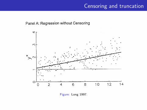
Figure: Long 1997.

Censoring and truncation
Figure: Long 1997.

Censoring and truncation
Truncation and censoring cause inconsistency in OLS estimates ofthe slope parameter (increasing n doesn’t solve the problem if theadditional observations come from the same data-generatingprocess).
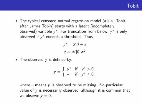
Tobit
• The typical censored normal regression model (a.k.a. Tobit,after James Tobin) starts with a latent (incompletelyobserved) variable y∗. For truncation from below, y∗ is onlyobserved if y∗ exceeds a threshold. Thus,
y∗ = x′β + ε,
ε = N [0, σ2]
• The observed y is defined by:
y =
{y∗ if y∗ > 0,– if y∗ ≤ 0,
where – means y is observed to be missing. No particularvalue of y is necessarily observed, although it is common thatwe observe y = 0.
Tobit
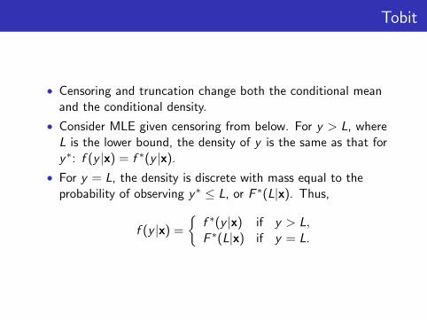
• Censoring and truncation change both the conditional meanand the conditional density.
• Consider MLE given censoring from below. For y > L, whereL is the lower bound, the density of y is the same as that fory∗: f (y |x) = f ∗(y |x).
• For y = L, the density is discrete with mass equal to theprobability of observing y∗ ≤ L, or F ∗(L|x). Thus,
f (y |x) =
{f ∗(y |x) if y > L,F ∗(L|x) if y = L.

Tobit
L92 REGRESSION MODELS
7.2. Truncated and Censored Distributions
Before formally considering the tobit model, we need some resultsabout truncated and censored normal distributions. These distributionsare at the foundation of most models for truncation and censoring. Re-sults are given for censoring and truncation on the left, which translatesinto censoring from below in the tobit model. Corresponding formu-las for censoring and truncation on the right, and both on the lett andon the right are available. For more details, see Johnson et al. (1994,pp.1,5G162) or Maddala (1983, pp. 365-368).
7.2.1. The Normal Distribution
To indicate that y* is distributed normally with mean p and variance02,we write y* - J{(p, oz).y* has the pdf:
r..*tr",d:#*o[-;(?)']which is plotted in panel A of Figure 7.3. The cdf is
ry'F(y* I t", o) : I f Ql t", o)dz : Pr(Y* < y*)
J--so that
Pr(Y* > 1l*) : 1 - F(Y* I t", o)
F(rlt",o) is the shaded region in panel A and t - F(r lpr, a) is theregion to the right of r.\Ponel A: Normol
Limited Outt
When trrthe simplifi
Any normabe written ibe written i
f0.lpand the cdf
So that,
Since the sr
two identiti,
These resulFor examplt
7.2.2. TheTr
When valcated normito consider
'6coo
pon.t S, Truncoted Ponel C: Censored
Censoring
Tl.LTpY' YIY)r
Figure 7.3. Normal Distribution With Tiuncation and
Figure: Long 1997.
Tobit
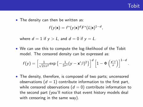
• The density can then be written as:
f (y |x) = f ∗(y |x)dF ∗(L|x)1−d ,
where d = 1 if y > L, and d = 0 if y = L.
• We can use this to compute the log-likelihood of the Tobitmodel. The censored density can be expressed as:
f (y) =[
1√2πσ2
exp{− 1
2σ2 (y − x′β)2}]d [
1− Φ(x′βσ
)]1−d.
• The density, therefore, is composed of two parts; uncensoredobservations (d = 1) contribute information to the first part,while censored observations (d = 0) contribute information tothe second part (you’ll notice that event history models dealwith censoring in the same way).

Tobit
• The Tobit MLE maximizes the censored log-likelihoodfunction:
lnLN(β, σ2) =N∑i
{di
(−1
2ln2π − 1
2lnσ2 − 1
2σ2(yi − x′iβ)2
)+ (1− di )ln
(1− Φ
(x′iβσ
))}

Tobit
Limitations:
• A major weakness of the Tobit MLE is its heavy reliance ondistributional assumptions
• Tobit assumes homoskedastic and normal errors. If either ofthose assumptions is violated, the Tobit MLE is inconsistent
• Consistent estimation with heteroskedastic errors can be doneby specifying a model for the error variance: σ2
i = exp(z′iγ).Consistency then requires correct specification of the errorvariance model
• Tobit restricts the censoring mechanism to be from the samemodel as that generating the outcome variable. On the otherhand, two-part models allow the censoring mechanism and theoutcome to be modeled using separate processes (e.g., theHeckman selection model and zero-inflated count models)
Heckman selection
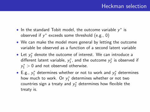
• In the standard Tobit model, the outcome variable y∗ isobserved if y∗ exceeds some threshold (e.g., 0)
• We can make the model more general by letting the outcomevariable be observed as a function of a second latent variable
• Let y∗2 denote the outcome of interest. We can introduce adifferent latent variable, y∗1 , and the outcome y∗2 is observed ify∗1 > 0 and not observed otherwise.
• E.g., y∗1 determines whether or not to work and y∗2 determineshow much to work. Or y∗1 determines whether or not twocountries sign a treaty and y∗2 determines how flexible thetreaty is.

Heckman selection
• A bivariate sample selection model then comprises a selectionequation:
y1 =
{1 if y∗1 > 0,0 if y∗1 ≤ 0.
• And an outcome equation:
y2 =
{y∗2 if y∗1 > 0,– if y∗1 ≤ 0.
• The standard model specifies a linear model for the latentvariables:
y∗1 = x′1β1 + ε1,y∗2 = x′2β2 + ε2.

Heckman selection
Where does selection bias come from?
E.g., suppose y∗2 , the outcome of interest, is wages and we want toestimate the effect of education on wages. y∗1 represents the utilityof entering the labor market or the propensity to work. We mightbelieve education also influences a person’s decision to work.

Heckman selection
There are two selection effects at work:
• First, more educated people might be more likely to enter thelabor force, and so we’ll have a sample of educated people.This non-random aspect of the sample is what is commonlymisunderstood to be the problem of ‘selection bias’ (seeSartori 2003).
• But this on its own does not bias the estimation of theoutcome equation.

Heckman selection
• The second selection effect is that some uneducated peoplewill choose to enter the work force. This is because theydecide that work is worthwhile because they have a high valueon some unmeasured variable, which is captured by ε1. Forexample, they may be smarter, but intelligence is notmeasured in our sample. That is, these people get into thesample not because they have high education, but becausethey have large error terms. The problem is that, whether ornot education is correlated with the unmeasured intelligencein the overall population, these two variables will be correlatedin the selected sample. If intelligence does lead to higherwages, then we will underestimate the effect of education onwages, because in the selected sample people with littleeducation are unusually smart.
Heckman selection
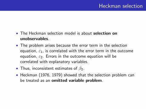
• The Heckman selection model is about selection onunobservables.
• The problem arises because the error term in the selectionequation, ε1, is correlated with the error term in the outcomeequation, ε2. Errors in the outcome equation will becorrelated with explanatory variables.
• Thus, inconsistent estimates of β2.
• Heckman (1976, 1979) showed that the selection problem canbe treated as an omitted variable problem.
Heckman selection
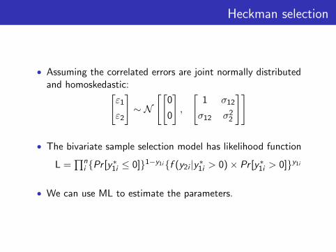
• Assuming the correlated errors are joint normally distributedand homoskedastic:[
ε1
ε2
]∼ N
[[0
0
],
[1 σ12
σ12 σ22
]]
• The bivariate sample selection model has likelihood function
L =∏n
i {Pr [y∗1i ≤ 0]}1−y1i{f (y2i |y∗1i > 0)× Pr [y∗1i > 0]}y1i
• We can use ML to estimate the parameters.

Heckman selection
• Heckman proposed a two-step estimator (LIML,limited-information maximum likelihood).
• For the subsample with a positive y∗2 , the conditionalexpectation of y∗2 is given by:
E (y∗2 |x2, y∗1 > 0) = x′2β2 + E (ε2|ε1 > −x′1β1)
• Given the assumption of joint normality and homoskedasticityof the errors, it can be shown that
E (ε2|ε1 > −x′1β1) = σ12σ1
φ(x′1β1/σ1)
Φ(−(x′1β1/σ1))
Heckman selection
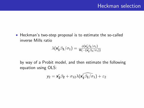
• Heckman’s two-step proposal is to estimate the so-calledinverse Mills ratio
λ(x′1β1/σ1) =φ(x′1β1/σ1)
Φ(−(x′1β1/σ1))
by way of a Probit model, and then estimate the followingequation using OLS:
y2 = x′2β2 + σ12λ( ̂x′1β1/σ1) + ε2

Heckman selection
• OLS standard errors will be wrong, though:• First, because of heteroskedasticity in ε2. Could correct for
heteroskedasticity by using robust s.e.’s, but...• Second, λ̂ is an estimator of λ, so the inverse Mills Ratio is
estimated with uncertainty. Need to take uncertainty intoaccount.
• Heckman 1979 provides a correction

Heckman selection
• Sample selection problem as a special case of omitted variableproblem (λ being the omitted variable).
• Heckman’s estimator is consistent if ε1 is normally distributedand ε2 is independent of λ.
• Two-step procedure has efficiency loss compared to FIML
• But needs less restrictive distributional assumptions thanFIML estimator (MLE requires joint normality of errors)
• Still, LIML estimates very sensitive to distributionalassumptions
• Distributional assumptions of LIML can be weakened evenfurther to permit semiparametric estimation
Heckman selection
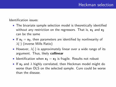
Identification issues:
• The bivariate sample selection model is theoretically identifiedwithout any restriction on the regressors. That is, x1 and x2can be the same
• If x1 = x2, then parameters are identified by nonlinearity ofλ(·) (inverse Mills Ratio)
• However, λ(·) is approximately linear over a wide range of itsargument. Thus, likely collinear
• Identification when x1 = x2 is fragile. Results not robust
• If x2 and λ highly correlated, then Heckman model might doworse than OLS on the selected sample. Cure could be worsethan the disease.
Heckman selection
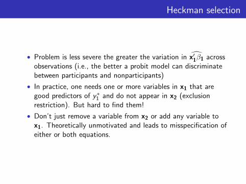
• Problem is less severe the greater the variation in x̂′1β1 acrossobservations (i.e., the better a probit model can discriminatebetween participants and nonparticipants)
• In practice, one needs one or more variables in x1 that aregood predictors of y∗1 and do not appear in x2 (exclusionrestriction). But hard to find them!
• Don’t just remove a variable from x2 or add any variable tox1. Theoretically unmotivated and leads to misspecification ofeither or both equations.

Models for sample selection
Software implementation:
• Tobit:• Stata: tobit• R: vglm function of the VGAM package
• Heckman selection model:• Stata: heckman (both FIML and two-step estimators)• R: heckit function of the sampleSelection package
Models for sample selection
Recommended reading:
• Long, Scott J. 1997. Regression Models for Categorical andLimited Dependent Variables. (Chapter 7)
• Cameron, A. Colin & Pravin K. Trivedi. 2005.Microeconometrics: Methods and Applications. (Chapter 16)
• Heckman, J. J. 1976. “The Common Structure of StatisticalModels of Truncation, Sample Selection and LimitedDependent Variables and a Simple Estimator for SuchModels.” Annals of Economic Social Measurement 5(4):475–492.
• Heckman, J. J. 1979. “Sample Selection Bias as aSpecification Error.” Econometrica 47(1): 53–161.
• Puhani, Patrick A. 2000. “The Heckman Correction forSample Selection and its Critique.” Journal of EconomicSurveys 14(1): 53–68.

Models for sample selection
Recommended reading (cont.):
• Winship, Christopher & Robert D. Mare. 1992. “Models forSample Selection Bias.” Annual Review of Sociology 18:327–350.
• Stolzenberg, Ross M. & Daniel A. Relles. 1997. “Tools forIntuition about Sample Selection Bias and its Correction.”American Sociological Review 62 (June 1997): 494–507.
• Vella, Francis. 1998. “Estimating Models with SampleSelection Bias: A Survey.” Journal of Human Resources33(1): 127–169.
• Sartori, Anne E. 2003. “An Estimator for SomeBinary-Outcome Selection Models Without ExclusionRestrictions.” Political Analysis 11: 111–138.
• Nooruddin, Irfan. 2002. “Modeling Selection Bias in Studiesof Sanctions Efficacy.” International Interactions 28: 59–75.