matrices handling in pdes resolution with matlab® · matrices handling in pdes resolution with...
TRANSCRIPT
Matrices handling in PDEs resolution with MATLAB R©
Riccardo [email protected]
Dipartimento di Ingegneria Meccanica e NavaleUniversità degli Studi Trieste, 34127 TRIESTE
April 6, 2016
Matrices handling in PDEs resolution with MATLAB April 6, 2016 1 / 64
OUTLINE
1 IntroductionExampleSource code files
2 1D case1D advection-diffusion problemDomain discretizationEquation discretizationBoundary conditions (BC)Sparse matrices handling
3 2D case2D advection-diffusion problem
Domain discretizationEquation discretizationBoundary conditions (BC)Coefficient matrix/RHS buildingSolution phase
4 Iterative methodsIntroduction2D Poisson problemDiscretizationIterative cycleSolution visualization
Matrices handling in PDEs resolution with MATLAB April 6, 2016 2 / 64
Introduction
In this part of CFD course we’ll see in practical terms how to handle the entities (matrices,vectors, etc.) that arise from the discretization of the fluid dynamics equations;
We’ll focus on the practical implementation of simple 1D and 2D steady-state cases;
The Finite Volume Method (FVM) will be used for the space discretization of theproblems, using Cartesian structured grids only;
MATLAB R© will be used as reference language, but a totally similar logic in themanipulation of the matrices is used in other languages (Scilab or Python for example,both free and Open source).
Matrices handling in PDEs resolution with MATLAB April 6, 2016 3 / 64
Example
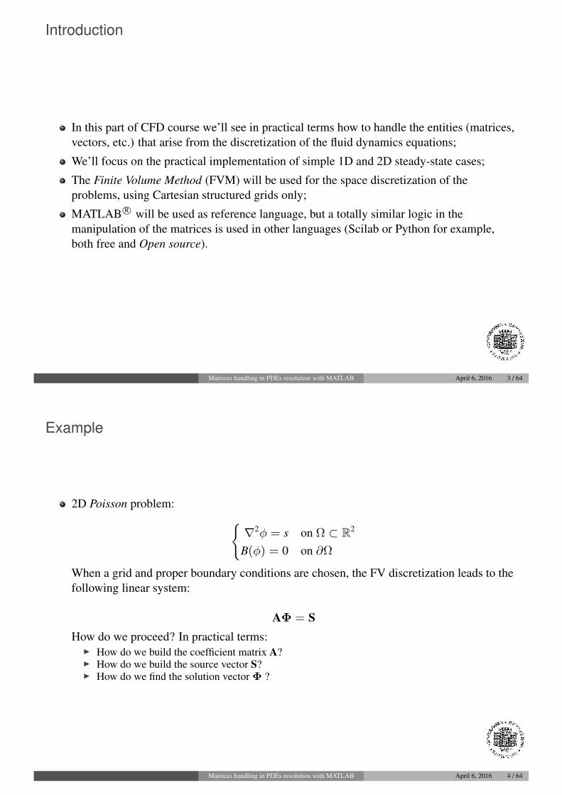
2D Poisson problem: ∇2φ = s on Ω ⊂ R2
B(φ) = 0 on ∂Ω
When a grid and proper boundary conditions are chosen, the FV discretization leads to thefollowing linear system:
AΦ = SHow do we proceed? In practical terms:
I How do we build the coefficient matrix A?I How do we build the source vector S?I How do we find the solution vector Φ ?
Matrices handling in PDEs resolution with MATLAB April 6, 2016 4 / 64
Source code files
MATLAB R© .m source code files used in these slides can be found at:
http://moodle2.units.it/
entering the TERMOFLUIDODINAMICA COMPUTAZIONALE course:
C1 AdvDiff_1D_Sparse.m1D advection-diffusion problem with direct solution (sparse matrix);
C2 AdvDiff_2D_Sparse.m2D advection-diffusion problem with direct and pcg solution (sparse matrix);
C3 Poisson_2D_Iter.m2D Poisson problem with iterative Jacobi and SOR methods (matrix-free).
Matrices handling in PDEs resolution with MATLAB April 6, 2016 5 / 64
1D advection-diffusion problem
1D steady-state advection-diffusion equation:
(ρwφ)x = (Γφx)x + s (1)
with constant properties ρ,Γ and constant velocity w;
Domain:Ω = [0, L]
Boundary conditions (BC):
Type Dirichlet BC Neumann BCEquation φ = φBC Γφx = J′′d,BC
Location x = 0 x = L
Matrices handling in PDEs resolution with MATLAB April 6, 2016 6 / 64
Variables
Variables definition:
% Constant properties (rho, gamma) and advection velocity (w)rho = 1 ;Gamma = 1 ;w = 1 ;
% Domain lengthL = 2*pi ;
% BC valuesphi_BC = 0 ;Jd_BC = 0 ;
Matrices handling in PDEs resolution with MATLAB April 6, 2016 7 / 64
Domain discretization
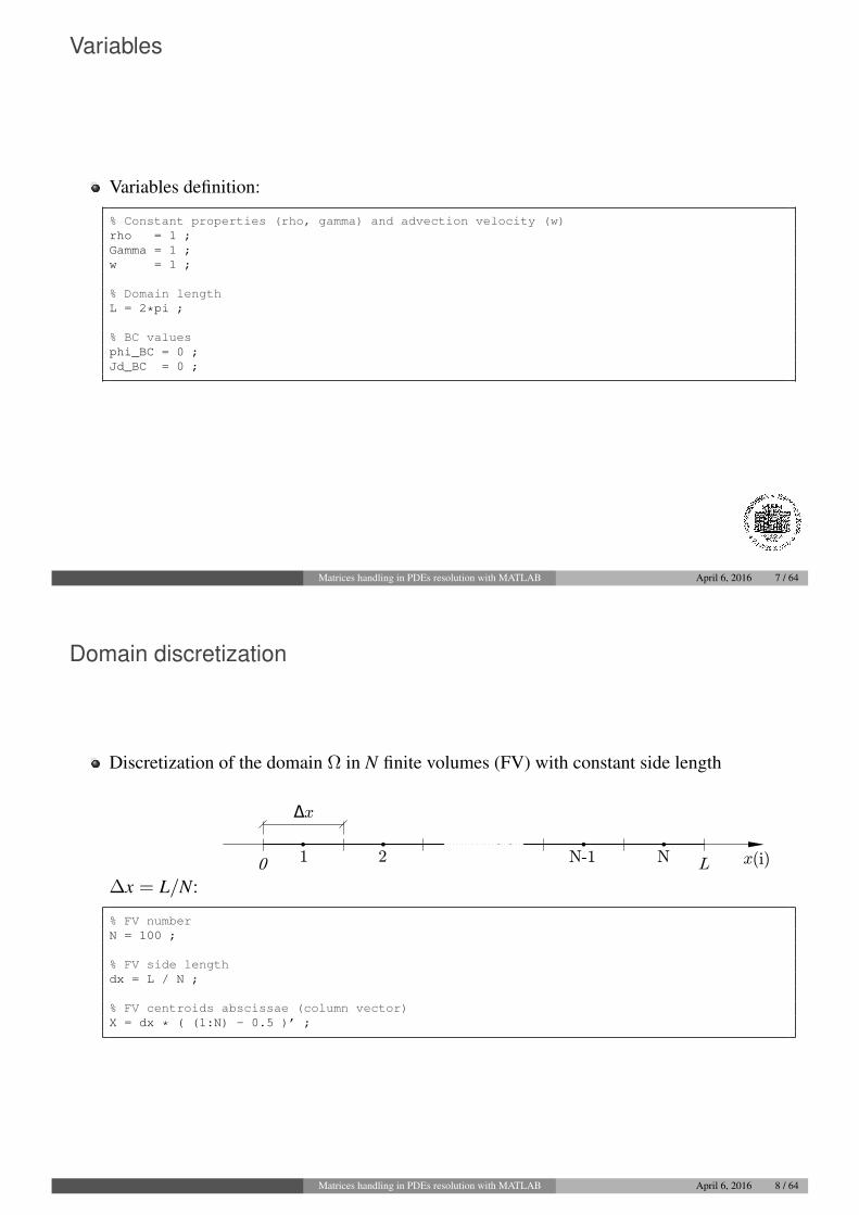
Discretization of the domain Ω in N finite volumes (FV) with constant side length
∆x = L/N:
x
Δx
0 L1 2 N-1 N (i)
% FV numberN = 100 ;
% FV side lengthdx = L / N ;
% FV centroids abscissae (column vector)X = dx * ( (1:N) - 0.5 )’ ;
Matrices handling in PDEs resolution with MATLAB April 6, 2016 8 / 64
Equation discretization
FV discretization of eq. (1) with 2nd order Central Differencing Scheme (CDS)approximation for both diffusive and advective fluxes:
AWφW + APφP + AEφE = SP (2)
% FV equation coefficients (constants for each FV)A_W = -rho * w / 2 - Gamma / dx ;A_E = rho * w / 2 - Gamma / dx ;A_P = -( A_W + A_E ) ;
Eq. (2) holds for each of the N finite volumes except for the first and the last FV, wherethis equation must be corrected because one of the neighbour cells doesn’t exist: BC willbe imposed using a ghost cell.
Matrices handling in PDEs resolution with MATLAB April 6, 2016 9 / 64
Equation discretization
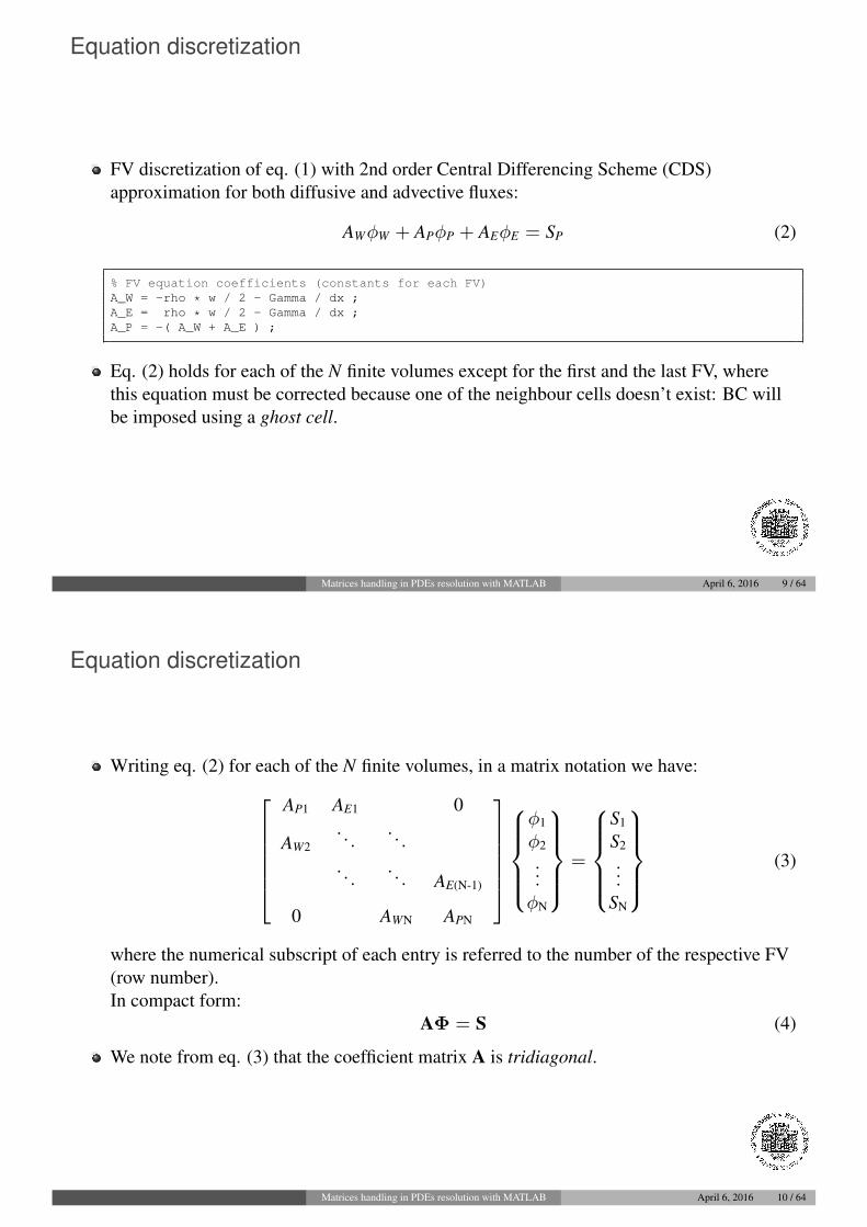
Writing eq. (2) for each of the N finite volumes, in a matrix notation we have:AP1 AE1 0
AW2. . .
. . .. . .
. . . AE(N-1)
0 AWN APN
φ1
φ2
...φN
=
S1
S2
...SN
(3)
where the numerical subscript of each entry is referred to the number of the respective FV(row number).In compact form:
AΦ = S (4)
We note from eq. (3) that the coefficient matrix A is tridiagonal.
Matrices handling in PDEs resolution with MATLAB April 6, 2016 10 / 64
Data organization
Considering the structure of eq. (3), it is appropriate to store the coefficients AWi,APi,AEi
and source terms Si (i = 1, . . . ,N) in column vectors D_W, D_P, D_E and S (N × 1matrices):
% Preparation of the 3 diagonals of A, stored as (column) vectorsD_W = A_W * ones( N , 1 ) ;D_P = A_P * ones( N , 1 ) ;D_E = A_E * ones( N , 1 ) ;
% RHS vector preparation (midpoint second order integration)S = s( X ) * dx ;
where the user defined function s(·) computes the source term s(·); therefore s( X ) isthe column vector of source term s evaluated at the FV centroids abscissæ X.
Matrices handling in PDEs resolution with MATLAB April 6, 2016 11 / 64
Boundary conditions
To impose BC at the boundary locations, we must correct the coefficients and source term forthe first and last FV using a ghost cell:
x = 0 (FV #1), Dirichlet BC:
φ(0) = φBC ⇒ φW + φP
2= φBC ⇒ φW = 2φBC − φP
Replacing φW in eq. (2) gives:
AW(2φBC − φP) + APφP + AEφE = SP (5)
Matrices handling in PDEs resolution with MATLAB April 6, 2016 12 / 64
Boundary conditions
Rearranging eq. (5) gives:
(AP − AW)︸ ︷︷ ︸AP1
φP + AEφE = SP − 2AWφBC︸ ︷︷ ︸S1
(6)
% Diagonals correction in order to impose BC% Left end ( x=0, i=1 ) (Dirichlet)D_P( 1 ) = D_P( 1 ) - D_W( 1 ) ;
S( 1 ) = S( 1 ) - 2 * D_W( 1 ) * phi_BC ;D_W( 1 ) = 0 ;
The last code line assigns a null value to the AW1 coefficient: this is not strictly needed, butit’s formally correct because the BC has been imposed and AW1 value is no longer needed.
Matrices handling in PDEs resolution with MATLAB April 6, 2016 13 / 64
Boundary conditions
x = L (FV #N), Neumann BC:
Γφx(L) = J′′d,BC ⇒ ΓφE − φP
∆x= J′′d,BC ⇒
⇒ φE = φP +∆xJ′′d,BC
Γ
Replacing φE in eq. (2) gives:
AWφW + APφP + AE(φP +∆xJ′′d,BC
Γ) = SP (7)
Matrices handling in PDEs resolution with MATLAB April 6, 2016 14 / 64
Boundary conditions
Rearranging eq. (7) gives:
AWφW + (AP + AE)︸ ︷︷ ︸APN
φP = SP − AE∆xJ′′d,BC
Γ︸ ︷︷ ︸SN
(8)
% Right end ( x=L, i=N ) (Neumann)D_P( N ) = D_P( N ) + D_E( N ) ;
S( N ) = S( N ) - D_E( N ) * dx * Jd_BC / Gamma ;D_E( N ) = 0 ;
Again, in the last code line we assign a null value to AEN because the BC has been imposedand AEN is no longer needed.
Matrices handling in PDEs resolution with MATLAB April 6, 2016 15 / 64
Sparsity
At this point we have all the variables needed to build the final matrix system, eq. (3);
As noted before, the coefficient matrix A is tridiagonal, i.e., only the main diagonal andthe first lower and upper diagonals have non null entries;
This particular sparse structure implies that the number of non null entries is proportionalto N (in this case exactly 3N − 2), while the total number of formal entries of A is N2;
The solution of a linear system with N unknowns requires, in general, a number ofoperations (and thus a time consumption) proportional to N3, while specific sparse solverscan reach an O(N) computational cost.
Matrices handling in PDEs resolution with MATLAB April 6, 2016 16 / 64
Sparse matrices
For example, if we choose N = 20000, the memory size required to naively store A wouldbe 8N2 bytes = 3.2 GB with double precision format, while the size of non null entries isonly 8 · 3N bytes = 480 kB;
A naive resolution of this system would take approximately 1 minute on a modern PC,while a generic sparse solver requires less than 1 ms;
It is clear that we must take advantage of the sparsity pattern of A to get acceptablecomputational resources consumption;
MATLAB R© can efficiently and easily handle sparse matrices, offering a wide set ofelementary sparse operations and, overall, sparse solvers;
Let’s see how to handle these particular matrices for our specific problem.
Matrices handling in PDEs resolution with MATLAB April 6, 2016 17 / 64
Building sparse banded matrices with spdiags()
We recognized the tridiagonal and sparse nature of coefficient matrix A, eq. (3);
Since these properties are particularly important and frequent in numerical problems,MATLAB R© offers the spdiags() function that allows to build sparse banded matricesfrom the diagonals:
A = spdiags( D , d , m , n )
A: sparse m×n banded matrix;D: matrix whose columns are the diagonals of A;d: vector of the shifts of each diagonal from the main diagonal.
Matrices handling in PDEs resolution with MATLAB April 6, 2016 18 / 64
Building sparse banded matrices with spdiags()
Let’s see how spdiags() works in practice with the D_W, D_P and D_E coefficientsvectors (diagonals) of our 1D problem; since we want a square N×N matrix A, m=n=N:
% Concatenation of the (column) vectors of the diagonals of AD = [ D_W D_P D_E ] ;
% Diagonals shifts from main diagonal% D_W is shifted -1 because it’s the first lower diagonal% D_P is shifted 0 because it’s the main diagonal% D_E is shifted 1 because it’s the first upper diagonald = [ -1 0 1 ] ;
% spdiags() callA_bad = spdiags( D , d , N , N ) ;
Matrices handling in PDEs resolution with MATLAB April 6, 2016 19 / 64
Building sparse banded matrices with spdiags()
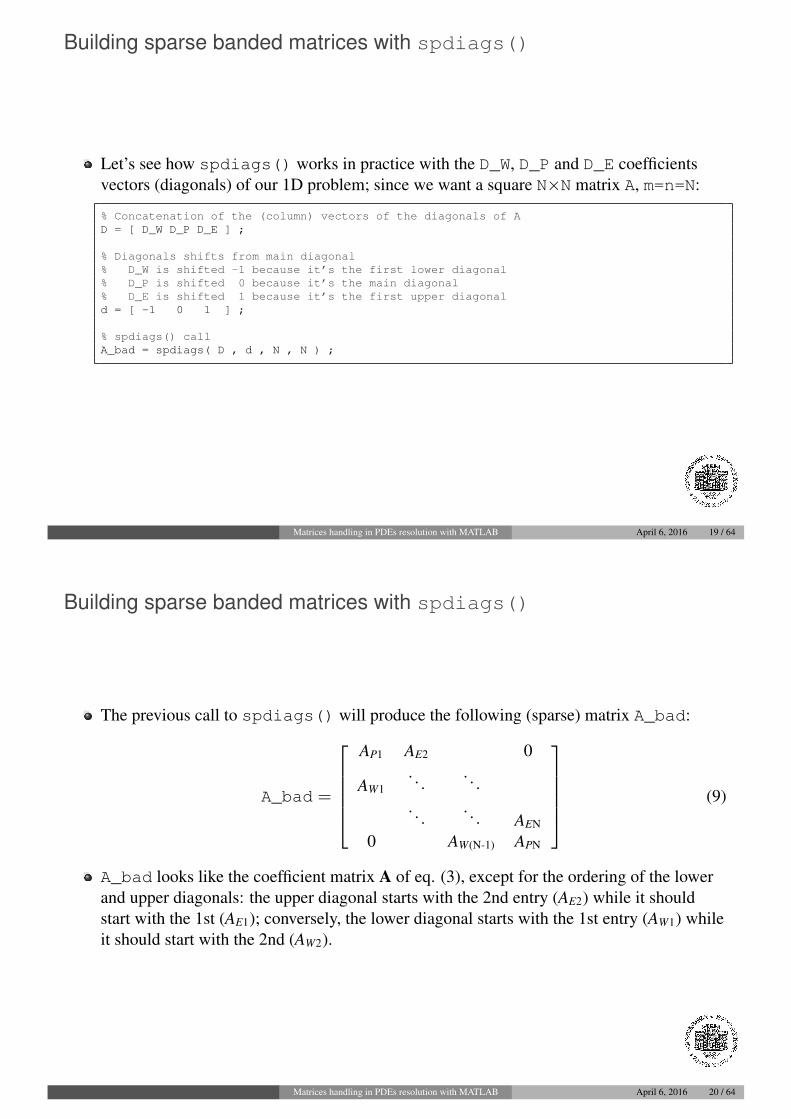
The previous call to spdiags() will produce the following (sparse) matrix A_bad:
A_bad =
AP1 AE2 0
AW1. . .
. . .. . .
. . . AEN
0 AW(N-1) APN
(9)
A_bad looks like the coefficient matrix A of eq. (3), except for the ordering of the lowerand upper diagonals: the upper diagonal starts with the 2nd entry (AE2) while it shouldstart with the 1st (AE1); conversely, the lower diagonal starts with the 1st entry (AW1) whileit should start with the 2nd (AW2).
Matrices handling in PDEs resolution with MATLAB April 6, 2016 20 / 64
Building sparse banded matrices with spdiags()
To fix this incorrect ordering of the diagonals, we can shift the elements in D_W and D_Evectors before the spdiags() call, using for example the circshift() commandwhich circularly shifts the elements of a matrix:
S_M = circshift( M , s , dim )
S_M: shifted matrix;M: matrix to be shifted;s: integer shift;
dim: dimension along which the shift is done.
If the matrix M to be shifted is a column vector (that’s our case) we can omit the thirdargument dim (= 1).
Matrices handling in PDEs resolution with MATLAB April 6, 2016 21 / 64
Building sparse banded matrices with spdiags()
We use circshift() with shift s=-1 for D_W because a negative shift is needed forthe lower diagonal, while a positive shift s=1 is needed for the upper diagonal D_E:
% Lower diagonal (West) and upper diagonal (East) shift.D_W = circshift( D_W , -1 ) ;D_E = circshift( D_E , 1 ) ;
Final (correct) spdiags() call:
% Concatenation of the (column) vectors of the diagonals of AD = [ D_W D_P D_E ] ;
% Diagonals shifts from main diagonald = [ -1 0 1 ] ;
% spdiags() call to build sparse tridiagonal AA = spdiags( D , d , N , N ) ;
Matrices handling in PDEs resolution with MATLAB April 6, 2016 22 / 64
Remarks
In our specific case where the AW , AP and AE coefficients are constants for each FV, theshift correction with circshift() could be avoided (D_W and D_E have constantentries), but it’s formally correct;
The circular property of circshift() is not strictly needed because the element beingcircularly shifted is anyway unused by spdiags();
The shift correction with circshift() could be anyway avoided inverting thediagonals order and taking the transpose (’):
% Concatenation of the (column vectors) diagonals of A, inverse orderD = [ D_E D_P D_W ] ;
% Diagonals shifts from main diagonald = [ -1 0 1 ] ;
% spdiags() call with transpose (’)A = spdiags( D , d , N , N )’ ;
Matrices handling in PDEs resolution with MATLAB April 6, 2016 23 / 64
Solution phase
At this point we have the (sparse) coefficient matrix A and the source vector S, thereforewe can calculate the solution vector Φ with the backslash \ operator:
% Direct solution (backslash \): A * phi = S => phi = A\Sphi = A\S ;
The \ operator is a powerful MATLAB R© function that allows the direct solution of linearsystems. It automatically checks for the input matrix nature (square/not square,dense/sparse, diagonal/tridiagonal/banded, Hermitian/non-Hermitian, real/complex, etc.)to choose the appropriate direct solver;
We’ll focus on the use of iterative solvers in the last section.
Matrices handling in PDEs resolution with MATLAB April 6, 2016 24 / 64
Solution plot
To graphically display the solution vector phi versus the X abscissæ vector we can usethe plot() function:
% Solution plotplot( X , phi ) ;
We can add labels to the axes:
% Naming axesxlabel( ’x’ ) ;ylabel( ’phi’ ) ;
There’s a large set of tunable properties for the graphics objects (Figures, Axes, Lines,etc.) to get aesthetically pleasant graphic plots.
Matrices handling in PDEs resolution with MATLAB April 6, 2016 25 / 64
Solution plot
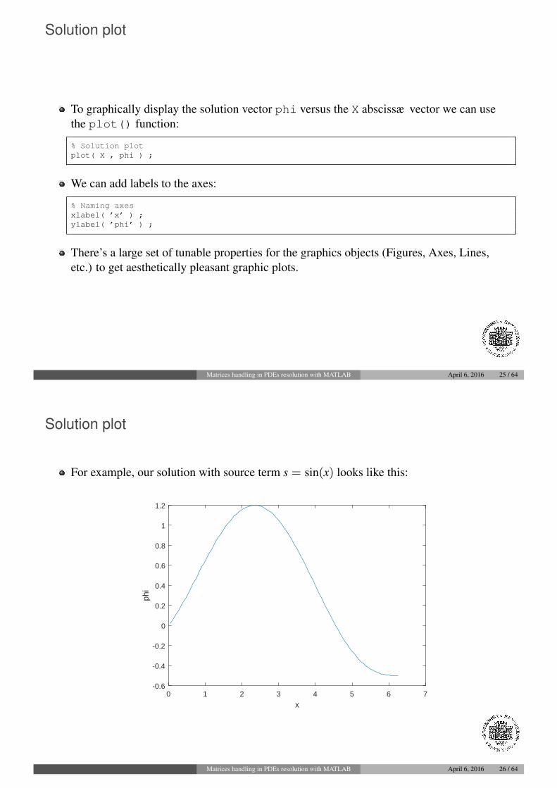
For example, our solution with source term s = sin(x) looks like this:
0 1 2 3 4 5 6 7
x
-0.6
-0.4
-0.2
0
0.2
0.4
0.6
0.8
1
1.2
phi
Matrices handling in PDEs resolution with MATLAB April 6, 2016 26 / 64
2D advection-diffusion problem
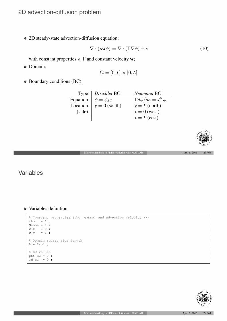
2D steady-state advection-diffusion equation:
∇ · (ρwφ) = ∇ · (Γ∇φ) + s (10)
with constant properties ρ,Γ and constant velocity w;
Domain:Ω = [0, L]× [0, L]
Boundary conditions (BC):
Type Dirichlet BC Neumann BCEquation φ = φBC Γdφ/dn = J′′d,BC
Location y = 0 (south) y = L (north)(side) x = 0 (west)
x = L (east)
Matrices handling in PDEs resolution with MATLAB April 6, 2016 27 / 64
Variables
Variables definition:
% Constant properties (rho, gamma) and advection velocity (w)rho = 1 ;Gamma = 1 ;w_x = 0 ;w_y = 1 ;
% Domain square side lengthL = 2*pi ;
% BC valuesphi_BC = 0 ;Jd_BC = 0 ;
Matrices handling in PDEs resolution with MATLAB April 6, 2016 28 / 64
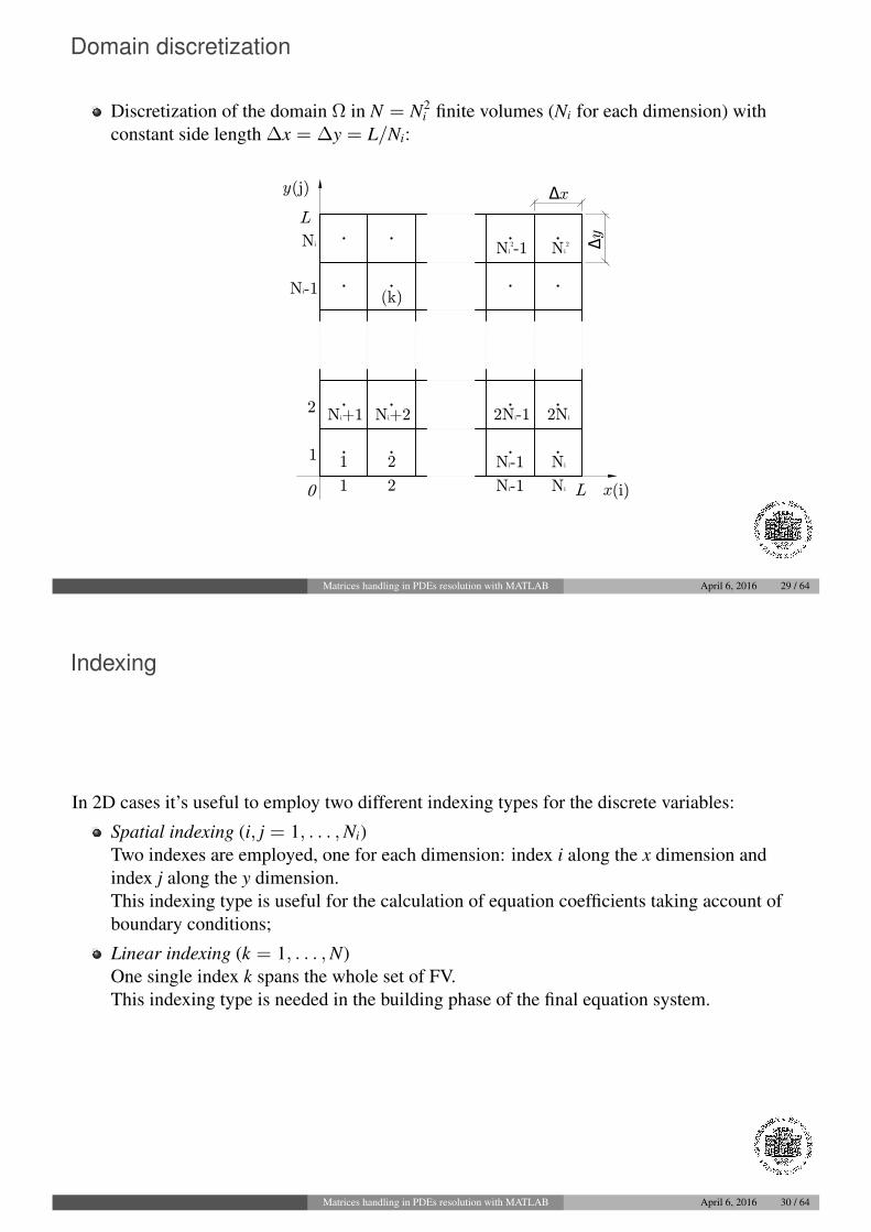
Domain discretization
Discretization of the domain Ω in N = N2i finite volumes (Ni for each dimension) with
constant side length ∆x = ∆y = L/Ni:
x
y
Δy
Δx
0
L
L
1
Ni+1
1
1
2
2
2
Ni+2 2Ni-1
Ni-1
Ni2-1
Ni-1
Ni-1
Ni Ni2
2Ni
Ni
Ni
(k)
(i)
(j)
Matrices handling in PDEs resolution with MATLAB April 6, 2016 29 / 64
Indexing
In 2D cases it’s useful to employ two different indexing types for the discrete variables:
Spatial indexing (i, j = 1, . . . ,Ni)Two indexes are employed, one for each dimension: index i along the x dimension andindex j along the y dimension.This indexing type is useful for the calculation of equation coefficients taking account ofboundary conditions;
Linear indexing (k = 1, . . . ,N)One single index k spans the whole set of FV.This indexing type is needed in the building phase of the final equation system.
Matrices handling in PDEs resolution with MATLAB April 6, 2016 30 / 64
Indexing
There’s a one-to-one correspondence for these indexing types:
k = i + Ni(j− 1) ;
i = 1 + (k − 1) mod Ni
j = 1 + (k − i )/Ni
However, we can ignore the previous formulas because we can implicitly pass from oneindexing to the other using reshape() command:
M_k = reshape( M_ij , N , 1 )M_ij = reshape( M_k , Ni , Ni )
M_k: N×1 column vector (linear indexing);M_ij: Ni×Ni matrix (spatial indexing);
N, Ni: N, Ni (total FV # and FV # for each dimension).
Matrices handling in PDEs resolution with MATLAB April 6, 2016 31 / 64
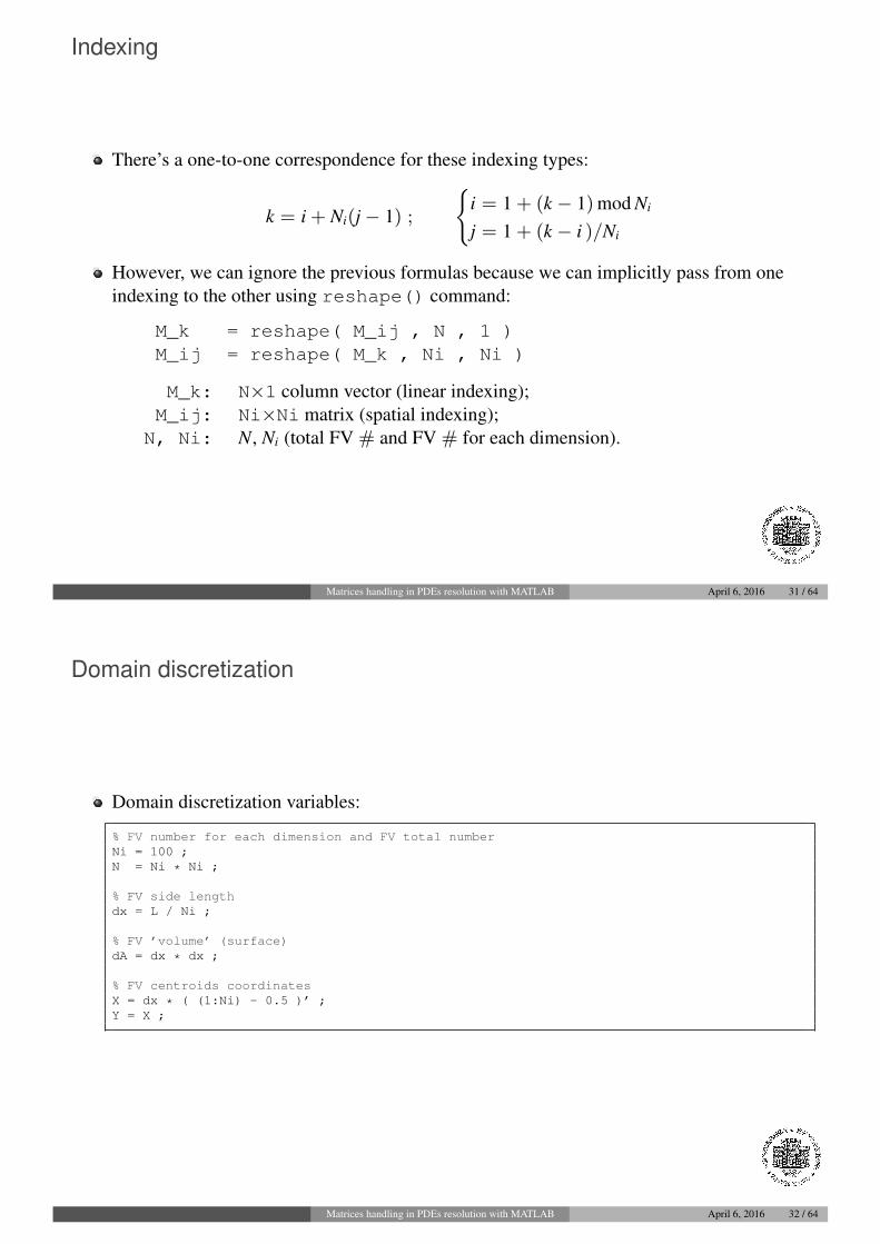
Domain discretization
Domain discretization variables:
% FV number for each dimension and FV total numberNi = 100 ;N = Ni * Ni ;
% FV side lengthdx = L / Ni ;
% FV ’volume’ (surface)dA = dx * dx ;
% FV centroids coordinatesX = dx * ( (1:Ni) - 0.5 )’ ;Y = X ;
Matrices handling in PDEs resolution with MATLAB April 6, 2016 32 / 64
Equation discretization
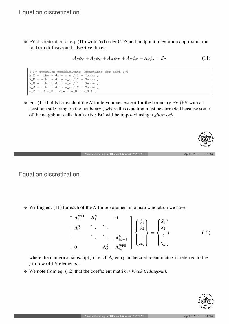
FV discretization of eq. (10) with 2nd order CDS and midpoint integration approximationfor both diffusive and advective fluxes:
APφP + AEφE + AWφW + ANφN + ASφS = SP (11)
% FV equation coefficients (constants for each FV)A_E = rho * dx * w_x / 2 - Gamma ;A_W = -rho * dx * w_x / 2 - Gamma ;A_N = rho * dx * w_y / 2 - Gamma ;A_S = -rho * dx * w_y / 2 - Gamma ;A_P = -( A_E + A_W + A_N + A_S ) ;
Eq. (11) holds for each of the N finite volumes except for the boundary FV (FV with atleast one side lying on the boubdary), where this equation must be corrected because someof the neighbour cells don’t exist: BC will be imposed using a ghost cell.
Matrices handling in PDEs resolution with MATLAB April 6, 2016 33 / 64
Equation discretization
Writing eq. (11) for each of the N finite volumes, in a matrix notation we have:AWPE
1 AN1 0
AS2
. . .. . .
. . .. . . AN
Ni−1
0 ASNi AWPE
Ni
φ1
φ2
...φN
=
S1
S2
...SN
(12)
where the numerical subscript j of each Aj entry in the coefficient matrix is referred to thej-th row of FV elements .
We note from eq. (12) that the coefficient matrix is block tridiagonal.
Matrices handling in PDEs resolution with MATLAB April 6, 2016 34 / 64
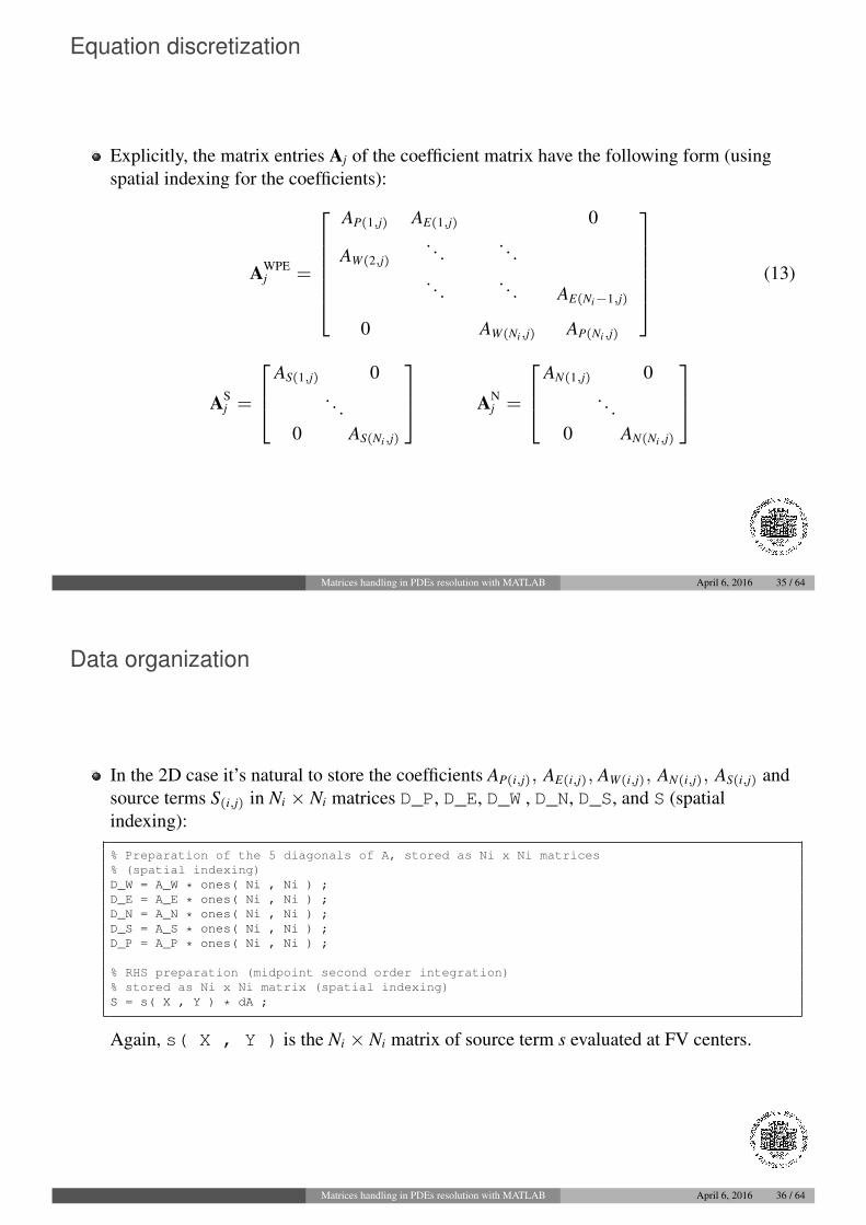
Equation discretization
Explicitly, the matrix entries Aj of the coefficient matrix have the following form (usingspatial indexing for the coefficients):
AWPEj =
AP(1,j) AE(1,j) 0
AW(2,j). . .
. . .. . .
. . . AE(Ni−1,j)
0 AW(Ni,j) AP(Ni,j)
(13)
ASj =
AS(1,j) 0. . .
0 AS(Ni,j)
ANj =
AN(1,j) 0. . .
0 AN(Ni,j)
Matrices handling in PDEs resolution with MATLAB April 6, 2016 35 / 64
Data organization
In the 2D case it’s natural to store the coefficients AP(i,j), AE(i,j), AW(i,j), AN(i,j), AS(i,j) andsource terms S(i,j) in Ni × Ni matrices D_P, D_E, D_W , D_N, D_S, and S (spatialindexing):
% Preparation of the 5 diagonals of A, stored as Ni x Ni matrices% (spatial indexing)D_W = A_W * ones( Ni , Ni ) ;D_E = A_E * ones( Ni , Ni ) ;D_N = A_N * ones( Ni , Ni ) ;D_S = A_S * ones( Ni , Ni ) ;D_P = A_P * ones( Ni , Ni ) ;
% RHS preparation (midpoint second order integration)% stored as Ni x Ni matrix (spatial indexing)S = s( X , Y ) * dA ;
Again, s( X , Y ) is the Ni × Ni matrix of source term s evaluated at FV centers.
Matrices handling in PDEs resolution with MATLAB April 6, 2016 36 / 64
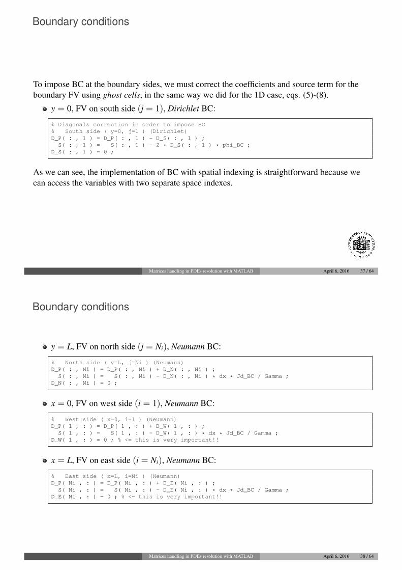
Boundary conditions
To impose BC at the boundary sides, we must correct the coefficients and source term for theboundary FV using ghost cells, in the same way we did for the 1D case, eqs. (5)-(8).
y = 0, FV on south side (j = 1), Dirichlet BC:
% Diagonals correction in order to impose BC% South side ( y=0, j=1 ) (Dirichlet)D_P( : , 1 ) = D_P( : , 1 ) - D_S( : , 1 ) ;
S( : , 1 ) = S( : , 1 ) - 2 * D_S( : , 1 ) * phi_BC ;D_S( : , 1 ) = 0 ;
As we can see, the implementation of BC with spatial indexing is straightforward because wecan access the variables with two separate space indexes.
Matrices handling in PDEs resolution with MATLAB April 6, 2016 37 / 64
Boundary conditions
y = L, FV on north side (j = Ni), Neumann BC:
% North side ( y=L, j=Ni ) (Neumann)D_P( : , Ni ) = D_P( : , Ni ) + D_N( : , Ni ) ;
S( : , Ni ) = S( : , Ni ) - D_N( : , Ni ) * dx * Jd_BC / Gamma ;D_N( : , Ni ) = 0 ;
x = 0, FV on west side (i = 1), Neumann BC:
% West side ( x=0, i=1 ) (Neumann)D_P( 1 , : ) = D_P( 1 , : ) + D_W( 1 , : ) ;
S( 1 , : ) = S( 1 , : ) - D_W( 1 , : ) * dx * Jd_BC / Gamma ;D_W( 1 , : ) = 0 ; % <= this is very important!!
x = L, FV on east side (i = Ni), Neumann BC:
% East side ( x=L, i=Ni ) (Neumann)D_P( Ni , : ) = D_P( Ni , : ) + D_E( Ni , : ) ;
S( Ni , : ) = S( Ni , : ) - D_E( Ni , : ) * dx * Jd_BC / Gamma ;D_E( Ni , : ) = 0 ; % <= this is very important!!
Matrices handling in PDEs resolution with MATLAB April 6, 2016 38 / 64
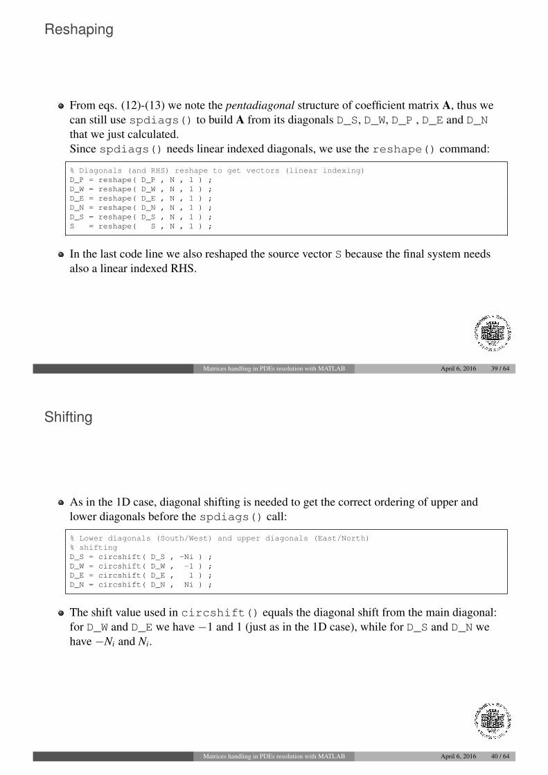
Reshaping
From eqs. (12)-(13) we note the pentadiagonal structure of coefficient matrix A, thus wecan still use spdiags() to build A from its diagonals D_S, D_W, D_P , D_E and D_Nthat we just calculated.Since spdiags() needs linear indexed diagonals, we use the reshape() command:
% Diagonals (and RHS) reshape to get vectors (linear indexing)D_P = reshape( D_P , N , 1 ) ;D_W = reshape( D_W , N , 1 ) ;D_E = reshape( D_E , N , 1 ) ;D_N = reshape( D_N , N , 1 ) ;D_S = reshape( D_S , N , 1 ) ;S = reshape( S , N , 1 ) ;
In the last code line we also reshaped the source vector S because the final system needsalso a linear indexed RHS.
Matrices handling in PDEs resolution with MATLAB April 6, 2016 39 / 64
Shifting
As in the 1D case, diagonal shifting is needed to get the correct ordering of upper andlower diagonals before the spdiags() call:
% Lower diagonals (South/West) and upper diagonals (East/North)% shiftingD_S = circshift( D_S , -Ni ) ;D_W = circshift( D_W , -1 ) ;D_E = circshift( D_E , 1 ) ;D_N = circshift( D_N , Ni ) ;
The shift value used in circshift() equals the diagonal shift from the main diagonal:for D_W and D_E we have −1 and 1 (just as in the 1D case), while for D_S and D_N wehave −Ni and Ni.
Matrices handling in PDEs resolution with MATLAB April 6, 2016 40 / 64
spdiags() call
At this point we have the 5 diagonals with correct indexing and correct ordering, so we cancall spdiags():
% Concatenation of the (column) vectors of the diagonals of AD = [ D_S D_W D_P D_E D_N ] ;
% Diagonals shifts from main diagonald = [ -Ni -1 0 1 Ni ] ;
% spdiags() call to build sparse pentadiagonal AA = spdiags( D , d , N , N ) ;
As we can see, the diagonals shifts from the main diagonal (d) are the same used incircshift() in the previous shifting phase.
Now we have sparse N × N pentadiagonal coefficient matrix A and N × 1 source termvector S, thus we can proceed to the solution phase.
Matrices handling in PDEs resolution with MATLAB April 6, 2016 41 / 64
Remarks
The shifting operation on D_W and D_E diagonals with circshift(), together with thenull assignation to the same diagonals in the BC imposition on west and east sides, iscrucial in 2D case even if the coefficients A are the same for every FV;
Again, the circular property of circshift() is not strictly needed;
The shift correction with circshift() could also be avoided inverting the diagonalsorder and taking the transpose (’):
% Concatenation of the (column vectors) diagonals of A, inverse orderD = [ D_N D_E D_P D_W D_S ] ;
% Diagonals shifts from main diagonald = [ -Ni -1 0 1 Ni ] ;
% spdiags() call with transpose (’)A = spdiags( D , d , N , N )’ ;
Matrices handling in PDEs resolution with MATLAB April 6, 2016 42 / 64
Solution phase
We can now calculate the solution vector Φ in the same way as in the 1D case, using thebackslash \ operator:
% Direct solution (backslash \): A * phi = S => phi = A\Sphi = A\S ;
Alternatively, we can compute an approximate solution using one of the MATLAB R©
built-in iterative solvers (pcg, minres, symmlq, etc.);
For example, we can use the Preconditioned Conjugate Gradient method (pcg) with anIncomplete Cholesky factorization (ichol) as preconditioner:
% PCG solution with Incomplete Cholesky factorization preconditionertol = relative tolerance on residual ;n_iter = maximum number of iterations ;L = ichol( A ) ;phi = pcg( A , S , tol , n_iter , L , L’ ) ;
Matrices handling in PDEs resolution with MATLAB April 6, 2016 43 / 64
Solution visualization: contour lines
For the graphical visualization of the solution, we need a spatial indexed solution phi(Ni × Ni matrix), thus we use reshape():
% Solution reshape to get again the spatial indexingphi = reshape( phi , [ Ni , Ni ] ) ;
We can display solution contour lines using contourf() command, which also fills thespaces with solution related colours (note the transpose (’) on phi to get the right axesorder):
% Contour line plot (orthogonal to the diffusive flux)contourf( X , Y , phi’ ) ;
% Naming axesxlabel( ’x’ ) ;ylabel( ’y’ ) ;
Matrices handling in PDEs resolution with MATLAB April 6, 2016 44 / 64
Solution visualization: 3D surface plot
We can also display a 3D solution surface using surf() command, which also coloursthe surface with solution related colours (again, note the transpose (’) on phi to get theright axes order):
% Surface plot on figure 2surf( X , Y , phi’ ) ;
% Naming axesxlabel( ’x’ ) ;ylabel( ’y’ ) ;zlabel( ’phi’ ) ;
With 3D surfaces it’s useful to tune some graphic properties (Edge Colors, Face Lighting,Lights, etc.) to get pretty and more understandable plots.
Matrices handling in PDEs resolution with MATLAB April 6, 2016 45 / 64
Solution visualization
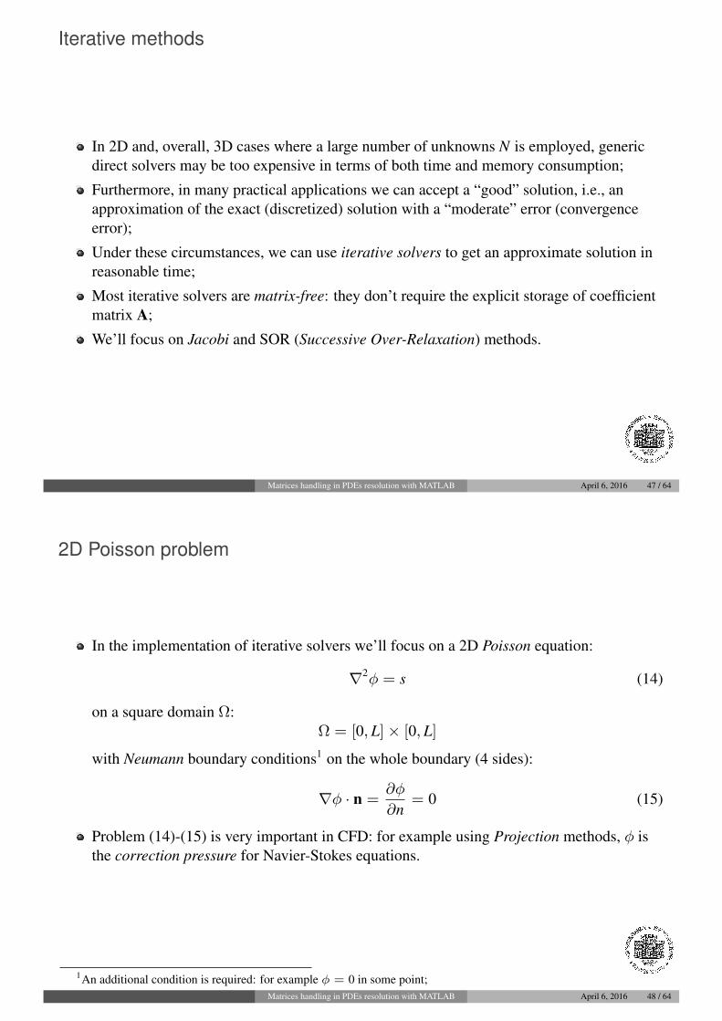
For example, with source term s = sin(x) sin(y) and some graphical tuning, our solutionlooks like this:
Matrices handling in PDEs resolution with MATLAB April 6, 2016 46 / 64
Iterative methods
In 2D and, overall, 3D cases where a large number of unknowns N is employed, genericdirect solvers may be too expensive in terms of both time and memory consumption;
Furthermore, in many practical applications we can accept a “good” solution, i.e., anapproximation of the exact (discretized) solution with a “moderate” error (convergenceerror);
Under these circumstances, we can use iterative solvers to get an approximate solution inreasonable time;
Most iterative solvers are matrix-free: they don’t require the explicit storage of coefficientmatrix A;
We’ll focus on Jacobi and SOR (Successive Over-Relaxation) methods.
Matrices handling in PDEs resolution with MATLAB April 6, 2016 47 / 64
2D Poisson problem
In the implementation of iterative solvers we’ll focus on a 2D Poisson equation:
∇2φ = s (14)
on a square domain Ω:Ω = [0, L]× [0, L]
with Neumann boundary conditions1 on the whole boundary (4 sides):
∇φ · n =∂φ
∂n= 0 (15)
Problem (14)-(15) is very important in CFD: for example using Projection methods, φ isthe correction pressure for Navier-Stokes equations.
1An additional condition is required: for example φ = 0 in some point;Matrices handling in PDEs resolution with MATLAB April 6, 2016 48 / 64
Domain discretization
We discretize the domain Ω in the same way as in the previous 2D case, with Ni finitevolumes for each dimension:
% Domain square side lengthL = 2*pi ;
% FV number for each dimensionNi = 100 ;
% FV side lengthdx = L / Ni ;
% FV ’volume’ (surface)dA = dx * dx ;
% FV centroids coordinatesX = dx * ( (1:Ni) - 0.5 )’ ;Y = X ;
Matrices handling in PDEs resolution with MATLAB April 6, 2016 49 / 64
Equation discretization
FV discretization of eq. (14) with 2nd order CDS and midpoint integration approximationfor diffusive flux:
APφP + AEφE + AWφW + ANφN + ASφS = SP (16)
% FV equation coefficients (constants for each FV)A_E = 1 ;A_W = 1 ;A_N = 1 ;A_S = 1 ;A_P = -4 ;
Eq. (16) holds for every FV, even for the boundary FV where coefficient corrections arenot needed anymore: BC will be enforced using ghost cells in a direct way.
Matrices handling in PDEs resolution with MATLAB April 6, 2016 50 / 64
Data organization
We store the solution phi as a (Ni + 2)× (Ni + 2) matrix (initialized with null values)because we need to store the ghost cells values explicitly, with spatial indexing:
% Solution matrix (spatial indexing + ghost cells)phi = zeros( Ni+2 , Ni+2 ) ;
We also need the vector k for the indexing in phi:
% Indexes of FV inside the domain (not ghost cells)k = 2 : (Ni+1) ;
For example, phi(k,k) is the Ni × Ni matrix of all φ values for the FV inside thedomain.
Matrices handling in PDEs resolution with MATLAB April 6, 2016 51 / 64
Data organization
Graphical representation of solution matrix phi:
1
1
2
2
W
Ni+1
Ni+1
Ni+2
Ni+2 i
k
k
jGhost cells
Matrices handling in PDEs resolution with MATLAB April 6, 2016 52 / 64
Data organization
The ghost cells values have the following access indexes:
Side Ghost cellsSouth phi(k,1)West phi(1,k)
North phi(k,Ni+2) or phi(k,end)East phi(Ni+2,k) or phi(end,k)
The source term is also spatial indexed and calculated with the classic midpoint secondorder integration approximation:
% Source term (midpoint second order integration)% Ni x Ni matrix (spatial indexing)S = s( X , Y ) * dA ;
Matrices handling in PDEs resolution with MATLAB April 6, 2016 53 / 64
Iterative cycle
The structure of the iterative cycle is the following:
% Number of iterationsn_iter = 1000 ;
% Iterative cyclefor iter = 1 : n_iter
UPDATE_SOLUTION() ;UPDATE_GHOST_CELLS_VALUES() ;
end
The function UPDATE_SOLUTION() updates the solution values in phi using a specificiterative method (Jacobi or SOR);
The function UPDATE_GHOST_CELLS_VALUES() only updates the ghost cells valuesin phi in order to enforce BC in a direct way.
Matrices handling in PDEs resolution with MATLAB April 6, 2016 54 / 64
Jacobi method
Jacobi method updates each unknown from the previous iteration values:
φn+1P =
SP − AEφnE − AWφ
nW − ANφ
nN − ASφ
nS
AP(17)
Since this method only requires φn values at previous iteration n, we can implement thisiteration in a matrix way:
UPDATE_SOLUTION():% Jacobi iterationngbrs = A_E*phi( k+1 , k ) + A_W*phi( k-1 , k ) + ...
A_N*phi( k , k+1 ) + A_S*phi( k , k-1 ) ;phi( k , k ) = ( S - ngbrs ) / A_P ;
Matrices handling in PDEs resolution with MATLAB April 6, 2016 55 / 64
Jacobi method
The previous matrix assignations used the vector k as index to access the neighbor cells inphi;
For example, phi(k+1,k) is the Ni × Ni matrix of all φE values, because the firstvectorial index is k+1;
We first calculate the Ni × Ni matrix ngbrs which contains the sum of the 4 neighbormatrices multiplied by their respective coefficient A; then we update the solution p(k,k)(Ni × Ni matrix);
The use of matrix assignations is efficient (no explicit for loops).
Matrices handling in PDEs resolution with MATLAB April 6, 2016 56 / 64
SOR method
Successive Over-Relaxation (SOR) method updates each unknown using the updatedvalues as soon as they’re available, with an over-relaxation step to accelerate theconvergence rate:
φn+1P = (1− ω)φn
P + (18)
+ ωSP − AEφ
nE − AWφ
n+1W − ANφ
nN − ASφ
n+1S
AP
Since this method requires φn+1 values at new iteration n + 1 as soon as they’re available,we can’t implement this iteration in a matrix way;
We have to explicitly write some for loops spanning over the solution matrix phi.
Matrices handling in PDEs resolution with MATLAB April 6, 2016 57 / 64
SOR method
The SOR code is therefore the following:
UPDATE_SOLUTION():% SOR over-relaxation parameterw = 1.6 ;
% SOR iterationfor i = k
for j = kngbrs = A_E*phi( i+1 , j ) + A_W*phi( i-1 , j ) + ...
A_N*phi( i , j+1 ) + A_S*phi( i , j-1 ) ;phi(i,j) = w*( S(i-1,j-1) - ngbrs )/A_P + (1-w)*phi(i,j) ;
endend
We used two for loops to span over the FV in the domain (i and j assume all the valuesin k);
In this case we update phi values one by one, not in a matrix way;
The source term S has to be accessed with i-1 and j-1 because it doesn’t have ghostcells.
Matrices handling in PDEs resolution with MATLAB April 6, 2016 58 / 64
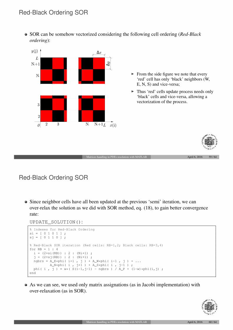
Red-Black Ordering SOR
SOR can be somehow vectorized considering the following cell ordering (Red-Blackordering):
x
y
Δy
Δx
0
L
L
2
2
3
3 Ni+1
Ni+1
Ni
Ni (i)
(j)
I From the side figure we note that every‘red’ cell has only ‘black’ neighbors (W,E, N, S) and vice-versa;
I Thus ‘red’ cells update process needs only‘black’ cells and vice-versa, allowing avectorization of the process.
Matrices handling in PDEs resolution with MATLAB April 6, 2016 59 / 64
Red-Black Ordering SOR
Since neighbor cells have all been updated at the previous ‘semi’ iteration, we canover-relax the solution as we did with SOR method, eq. (18), to gain better convergencerate:
UPDATE_SOLUTION():% Indexes for Red-Black Orderingsi = [ 0 1 0 1 ] ;sj = [ 0 1 1 0 ] ;
% Red-Black SOR iteration (Red cells: RB=1,2; Black cells: RB=3,4)for RB = 1 : 4
i = (2+si(RB)) : 2 : (Ni+1) ;j = (2+sj(RB)) : 2 : (Ni+1) ;ngbrs = A_E*phi( i+1 , j ) + A_W*phi( i-1 , j ) + ...
A_N*phi( i , j+1 ) + A_S*phi( i , j-1 ) ;phi( i , j ) = w*( S(i-1,j-1) - ngbrs ) / A_P + (1-w)*phi(i,j) ;
end
As we can see, we used only matrix assignations (as in Jacobi implementation) withover-relaxation (as in SOR).
Matrices handling in PDEs resolution with MATLAB April 6, 2016 60 / 64
Updating ghost cells
When the solution update phase is complete, we must update ghost cells values to directlyenforce BC; we proceed side by side:
UPDATE_GHOST_CELLS_VALUES():% Updating ’ghost cells’ values to enforce BC% South side ( y=0, j=1 ) (Neumann)phi( k , 1 ) = phi( k , 2 ) ;
% North side ( y=L, j=end ) (Neumann)phi( k , end ) = phi( k , end-1 ) ;
% West side ( x=0, i=1 ) (Neumann)phi( 1 , k ) = phi( 2 , k ) ;
% East side ( x=L, i=end ) (Neumann)phi( end , k ) = phi( end-1 , k ) ;
Matrices handling in PDEs resolution with MATLAB April 6, 2016 61 / 64
Solution shift
Since the Neumann BC (15) doesn’t specify any φ value, and Poisson equation (14) isinvariant under solution shiftings (φ+ c), we must enforce a fixed φ value on a point in thedomain to get an unique solution, for example φ(0, 0) = 0:
UPDATE_GHOST_CELLS_VALUES() continuation:
% Null solution on first FV [phi(2,2) = phi(x=0,y=0) to II order% because of BC]phi = phi - phi(2,2) ;
Matrices handling in PDEs resolution with MATLAB April 6, 2016 62 / 64
Solution extraction and visualization
At this point we accomplished the computation phase of the (approximate) solution of thediscrete FV equations;
If we’re not interested in the ghost cells values, we can now extract the solution values forthe FV inside the domain:
% Extraction of solution values for FV inside the domainphi = phi( k , k ) ;
Finally, we can display the solution as we did in the 2D advection-diffusion case usingcontourf() and surf() commands, for example.
Matrices handling in PDEs resolution with MATLAB April 6, 2016 63 / 64
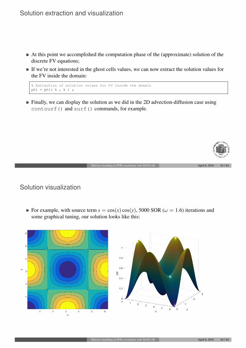
Solution visualization
For example, with source term s = cos(x) cos(y), 5000 SOR (ω = 1.6) iterations andsome graphical tuning, our solution looks like this:
Matrices handling in PDEs resolution with MATLAB April 6, 2016 64 / 64