matlab matrix and array operations
TRANSCRIPT
8/4/2019 Matlab Matrix and Array Operations
http://slidepdf.com/reader/full/matlab-matrix-and-array-operations 1/46
MATLAB array manipulation tips and tricks
Peter J. Acklam
E-mail: [email protected]
URL: http://home.online.no/~pjacklam
14th August 2002
8/4/2019 Matlab Matrix and Array Operations
http://slidepdf.com/reader/full/matlab-matrix-and-array-operations 2/46
Abstract
This document is intended to be a compilation of tips and tricks mainly related to
efficient ways of performing low-level array manipulation in MATLAB. Here, “manipu-
lation” means replicating and rotating arrays or parts of arrays, inserting, extracting,
permuting and shifting elements, generating combinations and permutations of ele-
ments, run-length encoding and decoding, multiplying and dividing arrays and calcu-
lating distance matrics and so forth. A few other issues regarding how to write fast
MATLAB code are also covered.
I’d like to thank the following people (in alphabetical order) for their suggestions, spotting typos and
other contributions they have made.
Ken Doniger and Dr. Denis Gilbert
Copyright © 2000–2002 Peter J. Acklam. All rights reserved.
Any material in this document may be reproduced or duplicated for personal or educational use.
MATLAB is a trademark of The MathWorks, Inc. (http://www.mathworks.com).
TEX is a trademark of the American Mathematical Society (http://www.ams.org).
Adobe PostScript and Adobe Acrobat Reader are trademarks of Adobe Systems Incorporated
(http://www.adobe.com).
The TEX source was written with the GNU Emacs text editor. The GNU Emacs home page ishttp://www.gnu.org/software/emacs/emacs.html.
The TEX source was formatted with AMS -LATEX to produce a DVI (device independent) file.
The PS (PostScript) version was created from the DVI file with dvips by Tomas Rokicki.
The PDF (Portable Document Format) version was created from the PS file with ps2pdf, a part of
Aladdin Ghostscript by Aladdin Enterprises.
The PS and PDF version may be viewed and printed with software available at the Ghostscript,
Ghostview and GSview Home Page, http://www.cs.wisc.edu/~ghost/index.html.
The PDF version may also be viewed and printed with Adobe Acrobat Reader, which is available at
http://www.adobe.com/products/acrobat/readstep.html.
8/4/2019 Matlab Matrix and Array Operations
http://slidepdf.com/reader/full/matlab-matrix-and-array-operations 3/46
CONTENTS 2
Contents
1 Introduction 4
1.1 The motivation for writing this document . . . . . . . . . . . . . . . . . . . . . . . 4
1.2 Who this document is for . . . . . . . . . . . . . . . . . . . . . . . . . . . . . . . . 5
1.3 Credit where credit is due . . . . . . . . . . . . . . . . . . . . . . . . . . . . . . . . 5
1.4 Errors and feedback . . . . . . . . . . . . . . . . . . . . . . . . . . . . . . . . . . . 5
1.5 Vectorization . . . . . . . . . . . . . . . . . . . . . . . . . . . . . . . . . . . . . . 5
2 Operators, functions and special characters 6
2.1 Operators . . . . . . . . . . . . . . . . . . . . . . . . . . . . . . . . . . . . . . . . 6
2.2 Built-in functions . . . . . . . . . . . . . . . . . . . . . . . . . . . . . . . . . . . . 7
2.3 M-file functions . . . . . . . . . . . . . . . . . . . . . . . . . . . . . . . . . . . . . 7
3 Basic array properties 83.1 Size . . . . . . . . . . . . . . . . . . . . . . . . . . . . . . . . . . . . . . . . . . . 8
3.1.1 Size along a specific dimension . . . . . . . . . . . . . . . . . . . . . . . . 8
3.1.2 Size along multiple dimension . . . . . . . . . . . . . . . . . . . . . . . . . 8
3.2 Dimensions . . . . . . . . . . . . . . . . . . . . . . . . . . . . . . . . . . . . . . . 9
3.2.1 Number of dimensions . . . . . . . . . . . . . . . . . . . . . . . . . . . . . 9
3.2.2 Singleton dimensions . . . . . . . . . . . . . . . . . . . . . . . . . . . . . . 9
3.3 Number of elements . . . . . . . . . . . . . . . . . . . . . . . . . . . . . . . . . . . 9
4 Array indices and subscripts 9
5 Creating vectors, matrices and arrays 9
5.1 Creating a constant array . . . . . . . . . . . . . . . . . . . . . . . . . . . . . . . . 9
5.1.1 When the class is determined by the scalar to replicate . . . . . . . . . . . . 95.1.2 When the class is stored in a string variable . . . . . . . . . . . . . . . . . . 10
5.2 Special vectors . . . . . . . . . . . . . . . . . . . . . . . . . . . . . . . . . . . . . 11
5.2.1 Uniformly spaced elements . . . . . . . . . . . . . . . . . . . . . . . . . . . 11
6 Shifting 11
6.1 Vectors . . . . . . . . . . . . . . . . . . . . . . . . . . . . . . . . . . . . . . . . . 11
6.2 Matrices and arrays . . . . . . . . . . . . . . . . . . . . . . . . . . . . . . . . . . . 11
7 Replicating elements and arrays 12
7.1 Creating a constant array . . . . . . . . . . . . . . . . . . . . . . . . . . . . . . . . 12
7.2 Replicating elements in vectors . . . . . . . . . . . . . . . . . . . . . . . . . . . . . 12
7.2.1 Replicate each element a constant number of times . . . . . . . . . . . . . . 12
7.2.2 Replicate each element a variable number of times . . . . . . . . . . . . . . 127.3 Using KRON for replicating elements . . . . . . . . . . . . . . . . . . . . . . . . . 12
7.3.1 KRON with an matrix of ones . . . . . . . . . . . . . . . . . . . . . . . . . 12
7.3.2 KRON with an identity matrix . . . . . . . . . . . . . . . . . . . . . . . . . 13
8 Reshaping arrays 13
8.1 Subdividing 2D matrix . . . . . . . . . . . . . . . . . . . . . . . . . . . . . . . . . 13
8.1.1 Create 4D array . . . . . . . . . . . . . . . . . . . . . . . . . . . . . . . . . 14
8.1.2 Create 3D array (columns first) . . . . . . . . . . . . . . . . . . . . . . . . . 14
8.1.3 Create 3D array (rows first) . . . . . . . . . . . . . . . . . . . . . . . . . . 14
8.1.4 Create 2D matrix (columns first, column output) . . . . . . . . . . . . . . . 15
8/4/2019 Matlab Matrix and Array Operations
http://slidepdf.com/reader/full/matlab-matrix-and-array-operations 4/46
CONTENTS 3
8.1.5 Create 2D matrix (columns first, row output) . . . . . . . . . . . . . . . . . 15
8.1.6 Create 2D matrix (rows first, column output) . . . . . . . . . . . . . . . . . 168.1.7 Create 2D matrix (rows first, row output) . . . . . . . . . . . . . . . . . . . 16
8.2 Stacking and unstacking pages . . . . . . . . . . . . . . . . . . . . . . . . . . . . . 17
9 Rotating matrices and arrays 17
9.1 Rotating 2D matrices . . . . . . . . . . . . . . . . . . . . . . . . . . . . . . . . . . 17
9.2 Rotating ND arrays . . . . . . . . . . . . . . . . . . . . . . . . . . . . . . . . . . . 17
9.3 Rotating ND arrays around an arbitrary axis . . . . . . . . . . . . . . . . . . . . . . 18
9.4 Block-rotating 2D matrices . . . . . . . . . . . . . . . . . . . . . . . . . . . . . . . 19
9.4.1 “Inner” vs “outer” block rotation . . . . . . . . . . . . . . . . . . . . . . . . 19
9.4.2 “Inner” block rotation 90 degrees counterclockwise . . . . . . . . . . . . . . 20
9.4.3 “Inner” block rotation 180 degrees . . . . . . . . . . . . . . . . . . . . . . . 21
9.4.4 “Inner” block rotation 90 degrees clockwise . . . . . . . . . . . . . . . . . . 22
9.4.5 “Outer” block rotation 90 degrees counterclockwise . . . . . . . . . . . . . 239.4.6 “Outer” block rotation 180 degrees . . . . . . . . . . . . . . . . . . . . . . 24
9.4.7 “Outer” block rotation 90 degrees clockwise . . . . . . . . . . . . . . . . . 25
9.5 Blocktransposing a 2D matrix . . . . . . . . . . . . . . . . . . . . . . . . . . . . . 25
9.5.1 “Inner” blocktransposing . . . . . . . . . . . . . . . . . . . . . . . . . . . . 25
9.5.2 “Outer” blocktransposing . . . . . . . . . . . . . . . . . . . . . . . . . . . . 26
10 Multiply arrays 26
10.1 Multiply each 2D slice with the same matrix (element-by-element) . . . . . . . . . . 26
10.2 Multiply each 2D slice with the same matrix (left) . . . . . . . . . . . . . . . . . . . 26
10.3 Multiply each 2D slice with the same matrix (right) . . . . . . . . . . . . . . . . . . 26
10.4 Multiply matrix with every element of a vector . . . . . . . . . . . . . . . . . . . . 27
10.5 Multiply each 2D slice with corresponding element of a vector . . . . . . . . . . . . 28
10.6 Outer product of all rows in a matrix . . . . . . . . . . . . . . . . . . . . . . . . . . 28
10.7 Keeping only diagonal elements of multiplication . . . . . . . . . . . . . . . . . . . 28
10.8 Products involving the Kronecker product . . . . . . . . . . . . . . . . . . . . . . . 29
11 Divide arrays 29
11.1 Divide each 2D slice with the same matrix (element-by-element) . . . . . . . . . . . 29
11.2 Divide each 2D slice with the same matrix (left) . . . . . . . . . . . . . . . . . . . . 29
11.3 Divide each 2D slice with the same matrix (right) . . . . . . . . . . . . . . . . . . . 30
12 Calculating distances 30
12.1 Euclidean distance . . . . . . . . . . . . . . . . . . . . . . . . . . . . . . . . . . . 30
12.2 Distance between two points . . . . . . . . . . . . . . . . . . . . . . . . . . . . . . 30
12.3 Euclidean distance vector . . . . . . . . . . . . . . . . . . . . . . . . . . . . . . . . 3112.4 Euclidean distance matrix . . . . . . . . . . . . . . . . . . . . . . . . . . . . . . . . 31
12.5 Special case when both matrices are identical . . . . . . . . . . . . . . . . . . . . . 31
12.6 Mahalanobis distance . . . . . . . . . . . . . . . . . . . . . . . . . . . . . . . . . . 32
13 Statistics, probability and combinatorics 33
13.1 Discrete uniform sampling with replacement . . . . . . . . . . . . . . . . . . . . . . 33
13.2 Discrete weighted sampling with replacement . . . . . . . . . . . . . . . . . . . . . 33
13.3 Discrete uniform sampling without replacement . . . . . . . . . . . . . . . . . . . . 33
13.4 Combinations . . . . . . . . . . . . . . . . . . . . . . . . . . . . . . . . . . . . . . 33
13.4.1 Counting combinations . . . . . . . . . . . . . . . . . . . . . . . . . . . . . 34
8/4/2019 Matlab Matrix and Array Operations
http://slidepdf.com/reader/full/matlab-matrix-and-array-operations 5/46
1 INTRODUCTION 4
13.4.2 Generating combinations . . . . . . . . . . . . . . . . . . . . . . . . . . . . 34
13.5 Permutations . . . . . . . . . . . . . . . . . . . . . . . . . . . . . . . . . . . . . . 3413.5.1 Counting permutations . . . . . . . . . . . . . . . . . . . . . . . . . . . . . 34
13.5.2 Generating permutations . . . . . . . . . . . . . . . . . . . . . . . . . . . . 34
14 Types of arrays 35
14.1 Numeric array . . . . . . . . . . . . . . . . . . . . . . . . . . . . . . . . . . . . . . 35
14.2 Real array . . . . . . . . . . . . . . . . . . . . . . . . . . . . . . . . . . . . . . . . 35
14.3 Identify real or purely imaginary elements . . . . . . . . . . . . . . . . . . . . . . . 35
14.4 Array of negative, non-negative or positive values . . . . . . . . . . . . . . . . . . . 36
14.5 Array of integers . . . . . . . . . . . . . . . . . . . . . . . . . . . . . . . . . . . . 36
14.6 Scalar . . . . . . . . . . . . . . . . . . . . . . . . . . . . . . . . . . . . . . . . . . 36
14.7 Vector . . . . . . . . . . . . . . . . . . . . . . . . . . . . . . . . . . . . . . . . . . 36
14.8 Matrix . . . . . . . . . . . . . . . . . . . . . . . . . . . . . . . . . . . . . . . . . . 37
14.9 Array slice . . . . . . . . . . . . . . . . . . . . . . . . . . . . . . . . . . . . . . . . 37
15 Logical operators and comparisons 37
15.1 List of logical operators . . . . . . . . . . . . . . . . . . . . . . . . . . . . . . . . . 37
15.2 Rules for logical operators . . . . . . . . . . . . . . . . . . . . . . . . . . . . . . . 37
15.3 Quick tests before slow ones . . . . . . . . . . . . . . . . . . . . . . . . . . . . . . 38
16 Miscellaneous 38
16.1 Accessing elements on the diagonal . . . . . . . . . . . . . . . . . . . . . . . . . . 38
16.2 Creating index vector from index limits . . . . . . . . . . . . . . . . . . . . . . . . 39
16.3 Matrix with different incremental runs . . . . . . . . . . . . . . . . . . . . . . . . . 40
16.4 Finding indices . . . . . . . . . . . . . . . . . . . . . . . . . . . . . . . . . . . . . 41
16.4.1 First non-zero element in each column . . . . . . . . . . . . . . . . . . . . . 41
16.4.2 First non-zero element in each row . . . . . . . . . . . . . . . . . . . . . . . 41
16.4.3 Last non-zero element in each row . . . . . . . . . . . . . . . . . . . . . . . 42
16.5 Run-length encoding and decoding . . . . . . . . . . . . . . . . . . . . . . . . . . . 43
16.5.1 Run-length encoding . . . . . . . . . . . . . . . . . . . . . . . . . . . . . . 43
16.5.2 Run-length decoding . . . . . . . . . . . . . . . . . . . . . . . . . . . . . . 43
16.6 Counting bits . . . . . . . . . . . . . . . . . . . . . . . . . . . . . . . . . . . . . . 44
Glossary 44
Index 44
1 Introduction
1.1 The motivation for writing this document
Since the early 1990’s I have been following the discussions in the main MATLAB newsgroup on
Usenet, comp.soft-sys.matlab. I realized that many of the postings in the group were about how to
manipulate arrays efficiently, which was something I had a great interest in. Since many of the the
same questions appeared again and again, I decided to start collecting what I thought were the most
interestings problems and solutions and see if I could compile them into one document. That was
the beginning of the document you are now reading.
8/4/2019 Matlab Matrix and Array Operations
http://slidepdf.com/reader/full/matlab-matrix-and-array-operations 6/46
1 INTRODUCTION 5
Instead of just providing a bunch of questions and answers, I have attempted to give general
answers, where possible. That way, a solution for a particular problem doesn’t just answer that oneproblem, but rather, that problem and all similar problems.
For a list of frequently asked questions, with answers, see see Peter Boettcher’s excellent MAT-
LAB FAQ which is posted to the news group comp.soft-sys.matlab regularely and is also available on
the web at http://www.mit.edu/~pwb/cssm/ .
1.2 Who this document is for
This document is mainly intended for the reader who knows the basics of MATLAB and would like
to dig further into the material. This document is more of a reference than a tutorial. The language
is rather technical although many of the terms used are explained. The index at the back should be
an aid in finding the explanation for a term unfamiliar to the reader.
1.3 Credit where credit is due
To the extent possible, I have given credit to what I believe is the author of a particular solution. In
many cases there is no single author, since several people have been tweaking and trimming each
other’s solutions. If I have given credit to the wrong person, please let me know.
In particular, I do not claim to be the sole author of a solution even though there is no other name
mentioned.
1.4 Errors and feedback
If you find errors, or have suggestions for improvements, or if there is anything you think should be
here but is not, please mail me and I will see what I can do. My address is on the front page of this
document.
1.5 Vectorization
The term “vectorization” is frequently associated with MATLAB. It is used and abused to the extent
that I think it deserves a section of its own in this introduction. I want to clearify what I put into the
term “vectorization”.
Strictly speaking, vectorization means to rewrite code so that one takes advantage of the vecto-
rization capabilities of the language being use. In particulaar, this means that one does scalar opera-
tions on multiple elements in one go, in stead of using a for-loop iterating over each element in an
array. For instance, the five lines
x = [ 1 2 3 4 5 ];
y = zeros(size(x));for i = 1:5
y(i) = x(i)^2;
end
may be written in the vectorized fashion
x = [ 1 2 3 4 5 ];
y = x.^2;
which is faster, more compact, and easier to read. An important aspect of vectorization is that the
operation being vectorized should be possible to do in parallel. The order in which the operation is
performed on each scalar should be irrelevant. This is the case with the example above. The order in
8/4/2019 Matlab Matrix and Array Operations
http://slidepdf.com/reader/full/matlab-matrix-and-array-operations 7/46
2 OPERATORS, FUNCTIONS AND SPECIAL CHARACTERS 6
which the elements are squared does not matter. With this rather strict definition of “vectorization”,
vectorized code is always faster than non-vectorized code.Some people use the term “vectorization” in the loose sense “removing a for-loop”, regardless
of what is inside the loop, but I will stick to the former, more strict definition.
2 Operators, functions and special characters
Clearly, it is important to know the language one intends to use. The language is described in the
manuals so I won’t repeat here what they say, but I strongly encourage the reader to type
help ops
at the command prompt and take a look at the list of operators, functions and special characters, and
look at the associated help pages.
When manipulating arrays in MATLAB there are some operators and functions that are particu-larely useful.
2.1 Operators
: The colon operator.
Type help colon for more information.
.’ Non-conjugate transpose.
Type help transpose for more information.
’ Complex conjugate transpose.
Type help ctranspose for more information.
8/4/2019 Matlab Matrix and Array Operations
http://slidepdf.com/reader/full/matlab-matrix-and-array-operations 8/46
2 OPERATORS, FUNCTIONS AND SPECIAL CHARACTERS 7
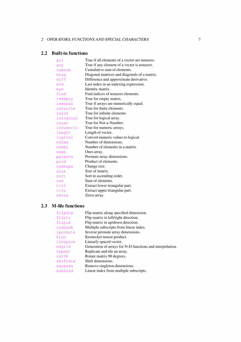
2.2 Built-in functions
all True if all elements of a vector are nonzero.any True if any element of a vector is nonzero.
cumsum Cumulative sum of elements.
diag Diagonal matrices and diagonals of a matrix.
diff Difference and approximate derivative.
end Last index in an indexing expression.
eye Identity matrix.
find Find indices of nonzero elements.
isempty True for empty matrix.
isequal True if arrays are numerically equal.
isfinite True for finite elements.
isinf True for infinite elements.
islogical True for logical array.isnan True for Not-a-Number.
isnumeric True for numeric arrays.
length Length of vector.
logical Convert numeric values to logical.
ndims Number of dimensions.
numel Number of elements in a matrix.
ones Ones array.
permute Permute array dimensions.
prod Product of elements.
reshape Change size.
size Size of matrix.
sort Sort in ascending order.
sum Sum of elements.tril Extract lower triangular part.
triu Extract upper triangular part.
zeros Zeros array.
2.3 M-file functions
flipdim Flip matrix along specified dimension.
fliplr Flip matrix in left/right direction.
flipud Flip matrix in up/down direction.
ind2sub Multiple subscripts from linear index.
ipermute Inverse permute array dimensions.
kron Kronecker tensor product.
linspace Linearly spaced vector.
ndgrid Generation of arrays for N-D functions and interpolation.
repmat Replicate and tile an array.
rot90 Rotate matrix 90 degrees.
shiftdim Shift dimensions.
squeeze Remove singleton dimensions.
sub2ind Linear index from multiple subscripts.
8/4/2019 Matlab Matrix and Array Operations
http://slidepdf.com/reader/full/matlab-matrix-and-array-operations 9/46
3 BASIC ARRAY PROPERTIES 8
3 Basic array properties
3.1 Size
The size of an array is a row vector with the length along all dimensions. The size of the array x can
be found with
sx = size(x); % size of x (along all dimensions)
The length of the size vector sx is the number of dimensions in x. That is, length(size(x))
is identical to ndims(x) (see section 3.2.1). No builtin array class in MATLAB has less than two
dimensions.
To change the size of an array without changing the number of elements, use reshape.
3.1.1 Size along a specific dimension
To get the length along a specific dimension dim, of the array x, use
size(x, dim) % size of x (along a specific dimension)
This will return one for all singleton dimensions (see section 3.2.2), and, in particular, it will return
one for all dim greater than ndims(x).
3.1.2 Size along multiple dimension
Sometimes one needs to get the size along multiple dimensions. It would be nice if we could use
size(x, dims), where dims is a vector of dimension numbers, but alas, size only allows the
dimension argument to be a scalar. We may of course use a for-loop solution:
siz = zeros(size(dims)); % initialize size vector to returnfor i = 1 : numel(dims) % loop over the elements in dims
siz(i) = size(x, dims(i)); % get the size along dimension
end % end loop
The above works, but a better solution is:
siz = ones(size(dims)); % initialize size vector to return
sx = size(x); % get size along all dimensions
k = dims <= ndims(x); % dimensions known not to be trailing singleton
siz(k) = sx(dims(k)); % insert size along dimensions of interest
Code like the following is sometimes seen, unfortunately. It might be more intuitive than the above,
but it is more fragile since it might use a lot more memory than necessary when dims contains a
large value.
sx = size(x); % get size along all dimensions
n = max(dims(:)) - ndims(x); % number of dimensions to append
sx = [ sx ones(1, n) ]; % pad size vector
siz = sx(dims); % extract dimensions of interest
An unlikely scenario, but imagine what happens if x and dims both are scalars and that dims is a
million. The above code would require more than 8 MB of memory. The suggested solution further
above requires a negligible amount of memory. There is no reason to write fragile code when it can
easily be avoided.
8/4/2019 Matlab Matrix and Array Operations
http://slidepdf.com/reader/full/matlab-matrix-and-array-operations 10/46
4 ARRAY INDICES AND SUBSCRIPTS 9
3.2 Dimensions
3.2.1 Number of dimensions
The number of dimensions of an array is the number of the highest non-singleton dimension (see
section 3.2.2) which is no less than two. Builtin arrays in MATLAB always have at least two dimen-
sions. The number of dimensions of an array x is
dx = ndims(x); % number of dimensions
In other words, ndims(x) is the largest value of dim, no less than two, for which size(x,dim)
is different from one. Here are a few examples
x = ones(2,1) % 2-dimensional
x = ones(2,1,1,1) % 2-dimensional
x = ones(1,0) % 2-dimensional
x = ones(1,2,3,0,0) % 5-dimensionalx = ones(2,3,0,0,1) % 4-dimensional
x = ones(3,0,0,1,2) % 5-dimensional
3.2.2 Singleton dimensions
A “singleton dimension” is a dimension along which the length is one. That is, if size(x,dim)
is one, then dim is a singleton dimension. If, in addition, dim is larger than ndims(x), then dim
is called a “trailing singleton dimension”. Trailing singleton dimensions are ignored by size and
ndims.
Singleton dimensions may be removed with squeeze. Removing singleton dimensions does
not change the number of elements in an array
Flipping an array along a singleton dimension is a null-operation, that is, it has no effect, itchanges nothing.
3.3 Number of elements
The number of elements in an array may be obtained with numel, e.g., numel(x) is the number
of elements in x. The number of elements is simply the product of the length along all dimensions,
that is, prod(size(x)). In particular, if the length along at least one dimension is zero, then the
array has zero elements regardless of the length along the other dimensions.
4 Array indices and subscripts
To be written.
5 Creating vectors, matrices and arrays
5.1 Creating a constant array
5.1.1 When the class is determined by the scalar to replicate
To create an array whose size is siz =[m n p q ...] and where each element has the value
val, use
X = repmat(val, siz);
8/4/2019 Matlab Matrix and Array Operations
http://slidepdf.com/reader/full/matlab-matrix-and-array-operations 11/46
5 CREATING VECTORS, MATRICES AND ARRAYS 10
Following are three other ways to achieve the same, all based on what repmat uses internally. Note
that for these to work, the array X should not already existX(prod(siz)) = val; % array of right class and num. of elements
X = reshape(X, siz); % reshape to specified size
X(:) = X(end); % fill ‘val’ into X (redundant if ‘val’ is zero)
If the size is given as a cell vector siz ={m n p q ...}, there is no need to reshape
X(siz{:}) = val; % array of right class and size
X(:) = X(end); % fill ‘val’ into ‘X’ (redundant if ‘val’ is zero)
If m, n, p, q, . . . are scalar variables, one may use
X(m,n,p,q) = val; % array of right class and size
X(:) = X(end); % fill ‘val’ into X (redundant if ‘val’ is zero)
The following way of creating a constant array is frequently used
X = val(ones(siz));
but this solution requires more memory since it creates an index array. Since an index array is used, it
only works if val is a variable, whereas the other solutions above also work when val is a function
returning a scalar value, e.g., if val is Inf or NaN:
X = NaN(ones(siz)); % this won’t work unless NaN is a variable
X = repmat(NaN, siz); % here NaN may be a function or a variable
Avoid using
X = val * ones(siz);
since it does unnecessary multiplications and only works for classes for which the multiplication
operator is defined.
5.1.2 When the class is stored in a string variable
To create an array of an arbitrary class cls, where cls is a character array (i.e., string) containing
the class name, use any of the above which allows val to be a function call and let val be
feval(cls, val)
As a special case, to create an array of class cls with only zeros, here are two ways
X = repmat(feval(cls, 0), siz); % a nice one-liner
X(prod(siz)) = feval(cls, 0);
X = reshape(X, siz);
Avoid using
X = feval(cls, zeros(siz)); % might require a lot more memory
since it first creates an array of class double which might require many times more memory than X
if an array of class cls requires less memory pr element than a double array.
8/4/2019 Matlab Matrix and Array Operations
http://slidepdf.com/reader/full/matlab-matrix-and-array-operations 12/46
6 SHIFTING 11
5.2 Special vectors
5.2.1 Uniformly spaced elements
To create a vector of uniformly spaced elements, use the linspace function or the : (colon)
operator:
X = linspace(lower, upper, n); % row vector
X = linspace(lower, upper, n).’; % column vector
X = lower : step : upper; % row vector
X = ( lower : step : upper ).’; % column vector
If the difference upper-lower is not a multiple of step, the last element of X, X(end), will be
less than upper. So the condition A(end) <= upper is always satisfied.
6 Shifting
6.1 Vectors
To shift and rotate the elements of a vector, use
X([ end 1:end-1 ]); % shift right/down 1 element
X([ end-k+1:end 1:end-k ]); % shift right/down k elements
X([ 2:end 1 ]); % shift left/up 1 element
X([ k+1:end 1:k ]); % shift left/up k elements
Note that these only work if k is non-negative. If k is an arbitrary integer one may use something
like
X( mod((1:end)-k-1, end)+1 ); % shift right/down k elements
X( mod((1:end)+k-1, end)+1 ); % shift left/up k element
where a negative k will shift in the opposite direction of a positive k.
6.2 Matrices and arrays
To shift and rotate the elements of an array X along dimension dim, first initialize a subscript cell
array with
idx = repmat({’:’}, ndims(X), 1); % initialize subscripts
n = size(X, dim); % length along dimension dim
then manipulate the subscript cell array as appropriate by using one of
idx{dim} = [ n 1:n-1 ]; % shift right/down/forwards 1 element
idx{dim} = [ n-k+1:n 1:n-k ]; % shift right/down/forwards k elements
idx{dim} = [ 2:n 1 ]; % shift left/up/backwards 1 element
idx{dim} = [ k+1:n 1:k ]; % shift left/up/backwards k elements
finally create the new array
Y = X(idx{:});
8/4/2019 Matlab Matrix and Array Operations
http://slidepdf.com/reader/full/matlab-matrix-and-array-operations 13/46
7 REPLICATING ELEMENTS AND ARRAYS 12
7 Replicating elements and arrays
7.1 Creating a constant array
See section 5.1.
7.2 Replicating elements in vectors
7.2.1 Replicate each element a constant number of times
Example Given
N = 3; A = [ 4 5 ]
create N copies of each element in A, so
B = [ 4 4 4 5 5 5 ]
Use, for instance,
B = A(ones(1,N),:);
B = B(:).’;
If A is a column-vector, use
B = A(:,ones(1,N)).’;
B = B(:);
Some people use
B = A( ceil( (1:N*length(A))/N ) );
but this requires unnecessary arithmetic. The only advantage is that it works regardless of whether
A is a row or column vector.
7.2.2 Replicate each element a variable number of times
See section 16.5.2 about run-length decoding.
7.3 Using KRON for replicating elements
7.3.1 KRON with an matrix of ones
Using kron with one of the arguments being a matrix of ones, may be used to replicate elements.
Firstly, since the replication is done by multiplying with a matrix of ones, it only works for classes
for which the multiplication operator is defined. Secondly, it is never necessary to perform any
multiplication to replicate elements. Hence, using kron is not the best way.
Assume A is a p-by-q matrix and that n is a non-negative integer.
Using KRON with a matrix of ones as first argument The expression
B = kron(ones(m,n), A);
may be computed more efficiently with
i = (1:p).’; i = i(:,ones(1,m));
j = (1:q).’; j = j(:,ones(1,n));
B = A(i,j);
or simply
B = repmat(A, [m n]);
8/4/2019 Matlab Matrix and Array Operations
http://slidepdf.com/reader/full/matlab-matrix-and-array-operations 14/46
8 RESHAPING ARRAYS 13
Using KRON with a matrix of ones as second argument The expression
B = kron(A, ones(m,n));
may be computed more efficiently with
i = 1:p; i = i(ones(1,m),:);
j = 1:q; j = j(ones(1,n),:);
B = A(i,j);
7.3.2 KRON with an identity matrix
Assume A is a p-by-q matrix and that n is a non-negative integer.
Using KRON with an identity matrix as second argument The expression
B = kron(A, eye(n));
may be computed more efficiently with
B = zeros(p, q, n, n);
B(:,:,1:n+1:n^2) = repmat(A, [1 1 n]);
B = permute(B, [3 1 4 2]);
B = reshape(B, [n*p n*q]);
or the following, which does not explicitly use either p or q
B = zeros([size(A) n n]);
B(:,:,1:n+1:n^2) = repmat(A, [1 1 n]);
B = permute(B, [3 1 4 2]);
B = reshape(B, n*size(A));
Using KRON with an identity matrix as first argument The expression
B = kron(eye(n), A);
may be computed more efficiently with
B = zeros(p, q, n, n);
B(:,:,1:n+1:n^2) = repmat(A, [1 1 n]);
B = permute(B, [1 3 2 4]);
B = reshape(B, [n*p n*q]);
or the following, which does not explicitly use either p or q
B = zeros([size(A) n n]);
B(:,:,1:n+1:n^2) = repmat(A, [1 1 n]);
B = permute(B, [1 3 2 4]);
B = reshape(B, n*size(A));
8 Reshaping arrays
8.1 Subdividing 2D matrix
Assume X is an m-by-n matrix.
8/4/2019 Matlab Matrix and Array Operations
http://slidepdf.com/reader/full/matlab-matrix-and-array-operations 15/46
8 RESHAPING ARRAYS 14
8.1.1 Create 4D array
To create a p-by-q-by-m/p-by-n/q array Y where the i,j submatrix of X is Y(:,:,i,j), use
Y = reshape( X, [ p m/p q n/q ] );
Y = p e r m u t e ( Y , [ 1 3 2 4 ] ) ;
Now,
X = [ Y(:,:,1,1) Y(:,:,1,2) ... Y(:,:,1,n/q)
Y(:,:,2,1) Y(:,:,2,2) ... Y(:,:,2,n/q)
... ... ... ...
Y(:,:,m/p,1) Y(:,:,m/p,2) ... Y(:,:,m/p,n/q) ];
To restore X from Y use
X = p e r m u t e ( Y , [ 1 3 2 4 ] ) ;
X = reshape( X, [ m n ] );
8.1.2 Create 3D array (columns first)
Assume you want to create a p-by-q-by-m*n/(p*q) array Y where the i,j submatrix of X is
Y(:,:,i+(j-1)*m/p). E.g., if A, B, C and D are p-by-q matrices, convert
X = [ A B
C D ] ;
into
Y = cat( 3, A, C, B, D );
use
Y = reshape( X, [ p m/p q n/q ] );
Y = p e r m u t e ( Y , [ 1 3 2 4 ] ) ;
Y = reshape( Y, [ p q m*n/(p*q) ] )
Now,
X = [ Y(:,:,1) Y(:,:,m/p+1) ... Y(:,:,(n/q-1)*m/p+1)
Y(:,:,2) Y(:,:,m/p+2) ... Y(:,:,(n/q-1)*m/p+2)
... ... ... ...
Y(:,:,m/p) Y(:,:,2*m/p) ... Y(:,:,n/q*m/p) ];
To restore X from Y use
X = reshape( Y, [ p q m/p n/q ] );
X = p e r m u t e ( X , [ 1 3 2 4 ] ) ;
X = reshape( X, [ m n ] );
8.1.3 Create 3D array (rows first)
Assume you want to create a p-by-q-by-m*n/(p*q) array Y where the i,j submatrix of X is
Y(:,:,j+(i-1)*n/q). E.g., if A, B, C and D are p-by-q matrices, convert
X = [ A B
C D ] ;
8/4/2019 Matlab Matrix and Array Operations
http://slidepdf.com/reader/full/matlab-matrix-and-array-operations 16/46
8 RESHAPING ARRAYS 15
into
Y = cat( 3, A, B, C, D );
use
Y = reshape( X, [ p m/p n ] );
Y = permute( Y, [ 1 3 2 ] );
Y = reshape( Y, [ p q m*n/(p*q) ] );
Now,
X = [ Y(:,:,1) Y(:,:,2) ... Y(:,:,n/q)
Y(:,:,n/q+1) Y(:,:,n/q+2) ... Y(:,:,2*n/q)
... ... ... ...
Y(:,:,(m/p-1)*n/q+1) Y(:,:,(m/p-1)*n/q+2) ... Y(:,:,m/p*n/q) ];
To restore X from Y use
X = reshape( Y, [ p n m/p ] );
X = permute( X, [ 1 3 2 ] );
X = reshape( X, [ m n ] );
8.1.4 Create 2D matrix (columns first, column output)
Assume you want to create a m*n/q-by-q matrix Y where the submatrices of X are concatenated
(columns first) vertically. E.g., if A, B, C and D are p-by-q matrices, convert
X = [ A B
C D ] ;
into
Y = [ A
C
B
D ];
use
Y = reshape( X, [ m q n/q ] );
Y = permute( Y, [ 1 3 2 ] );
Y = reshape( Y, [ m*n/q q ] );
To restore X from Y use
X = reshape( Y, [ m n/q q ] );
X = permute( X, [ 1 3 2 ] );
X = reshape( X, [ m n ] );
8.1.5 Create 2D matrix (columns first, row output)
Assume you want to create a p-by-m*n/p matrix Y where the submatrices of X are concatenated
(columns first) horizontally. E.g., if A, B, C and D are p-by-q matrices, convert
X = [ A B
C D ] ;
8/4/2019 Matlab Matrix and Array Operations
http://slidepdf.com/reader/full/matlab-matrix-and-array-operations 17/46
8 RESHAPING ARRAYS 16
into
Y = [ A C B D ];
use
Y = reshape( X, [ p m/p q n/q ] )
Y = p e r m u t e ( Y , [ 1 3 2 4 ] ) ;
Y = reshape( Y, [ p m*n/p ] );
To restore X from Y use
Z = reshape( Y, [ p q m/p n/q ] );
Z = p e r m u t e ( Z , [ 1 3 2 4 ] ) ;
Z = reshape( Z, [ m n ] );
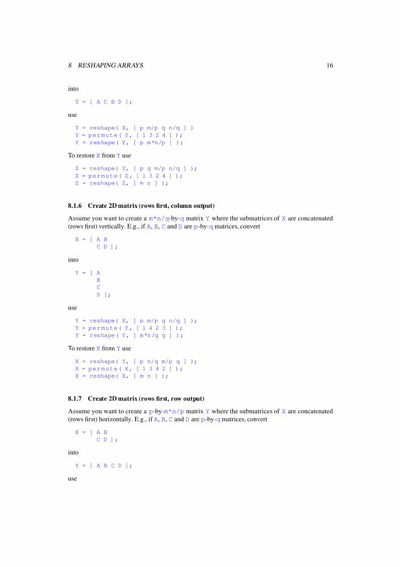
8.1.6 Create 2D matrix (rows first, column output)
Assume you want to create a m*n/q-by-q matrix Y where the submatrices of X are concatenated
(rows first) vertically. E.g., if A, B, C and D are p-by-q matrices, convert
X = [ A B
C D ] ;
into
Y = [ A
B
C
D ];
use
Y = reshape( X, [ p m/p q n/q ] );
Y = p e r m u t e ( Y , [ 1 4 2 3 ] ) ;
Y = reshape( Y, [ m*n/q q ] );
To restore X from Y use
X = reshape( Y, [ p n/q m/p q ] );
X = p e r m u t e ( X , [ 1 3 4 2 ] ) ;
X = reshape( X, [ m n ] );
8.1.7 Create 2D matrix (rows first, row output)
Assume you want to create a p-by-m*n/p matrix Y where the submatrices of X are concatenated
(rows first) horizontally. E.g., if A, B, C and D are p-by-q matrices, convert
X = [ A B
C D ] ;
into
Y = [ A B C D ];
use
8/4/2019 Matlab Matrix and Array Operations
http://slidepdf.com/reader/full/matlab-matrix-and-array-operations 18/46
9 ROTATING MATRICES AND ARRAYS 17
Y = reshape( X, [ p m/p n ] );
Y = permute( Y, [ 1 3 2 ] );
Y = reshape( Y, [ p m*n/p ] );
To restore X from Y use
X = reshape( Y, [ p n m/p ] );
X = permute( X, [ 1 3 2 ] );
X = reshape( X, [ m n ] );
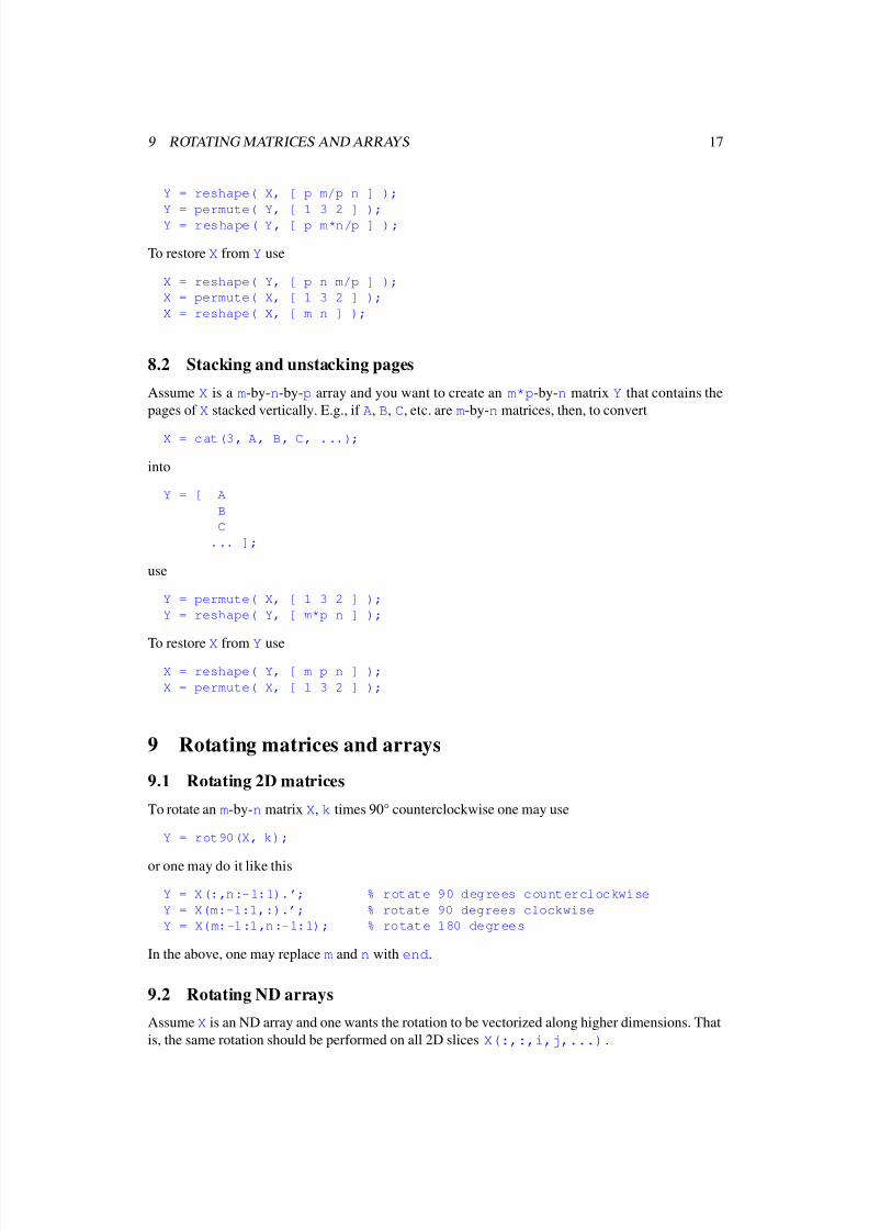
8.2 Stacking and unstacking pages
Assume X is a m-by-n-by-p array and you want to create an m*p-by-n matrix Y that contains the
pages of X stacked vertically. E.g., if A, B, C, etc. are m-by-n matrices, then, to convert
X = cat(3, A, B, C, ...);
into
Y = [ A
B
C
... ];
use
Y = permute( X, [ 1 3 2 ] );
Y = reshape( Y, [ m*p n ] );
To restore X from Y use
X = reshape( Y, [ m p n ] );
X = permute( X, [ 1 3 2 ] );
9 Rotating matrices and arrays
9.1 Rotating 2D matrices
To rotate an m-by-n matrix X, k times 90° counterclockwise one may use
Y = rot90(X, k);
or one may do it like this
Y = X(:,n:-1:1).’; % rotate 90 degrees counterclockwise
Y = X(m:-1:1,:).’; % rotate 90 degrees clockwise
Y = X(m:-1:1,n:-1:1); % rotate 180 degrees
In the above, one may replace m and n with end.
9.2 Rotating ND arrays
Assume X is an ND array and one wants the rotation to be vectorized along higher dimensions. That
is, the same rotation should be performed on all 2D slices X(:,:,i,j,...).
8/4/2019 Matlab Matrix and Array Operations
http://slidepdf.com/reader/full/matlab-matrix-and-array-operations 19/46
9 ROTATING MATRICES AND ARRAYS 18
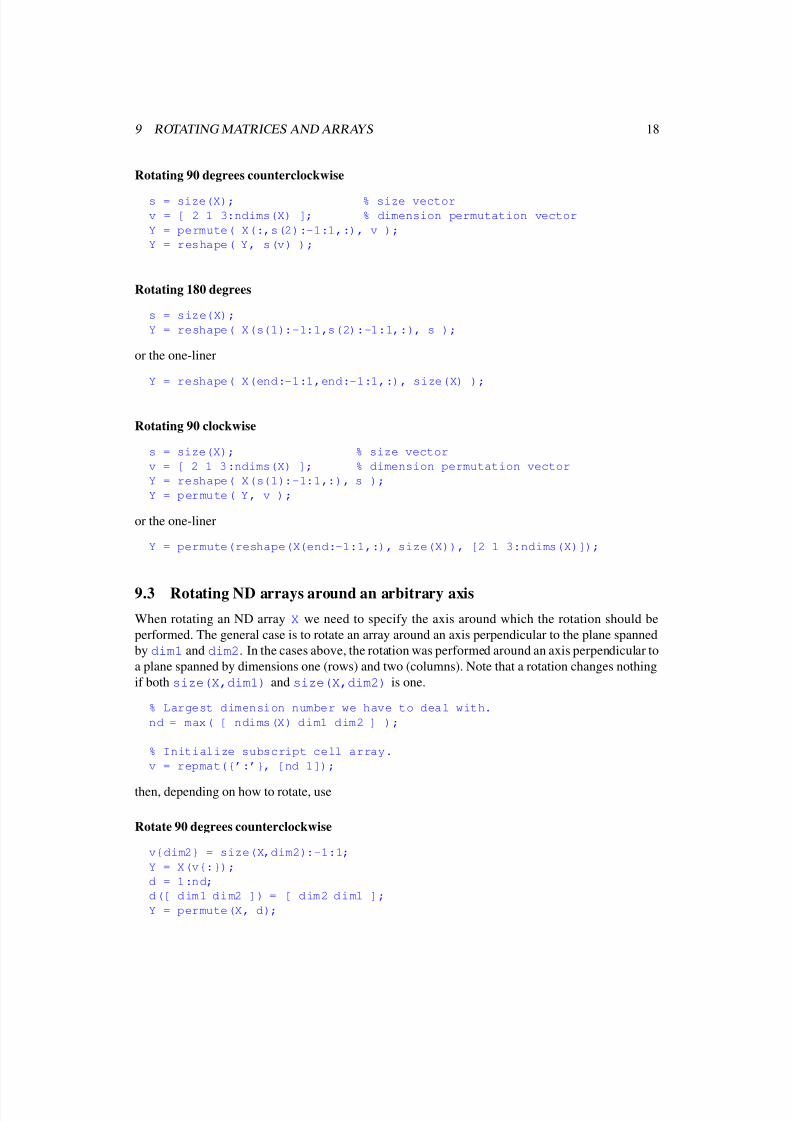
Rotating 90 degrees counterclockwise
s = size(X); % size vector
v = [ 2 1 3:ndims(X) ]; % dimension permutation vector
Y = permute( X(:,s(2):-1:1,:), v );
Y = reshape( Y, s(v) );
Rotating 180 degrees
s = size(X);
Y = reshape( X(s(1):-1:1,s(2):-1:1,:), s );
or the one-liner
Y = reshape( X(end:-1:1,end:-1:1,:), size(X) );
Rotating 90 clockwise
s = size(X); % size vector
v = [ 2 1 3:ndims(X) ]; % dimension permutation vector
Y = reshape( X(s(1):-1:1,:), s );
Y = permute( Y, v );
or the one-liner
Y = permute(reshape(X(end:-1:1,:), size(X)), [2 1 3:ndims(X)]);
9.3 Rotating ND arrays around an arbitrary axis
When rotating an ND array X we need to specify the axis around which the rotation should be
performed. The general case is to rotate an array around an axis perpendicular to the plane spanned
by dim1 and dim2. In the cases above, the rotation was performed around an axis perpendicular to
a plane spanned by dimensions one (rows) and two (columns). Note that a rotation changes nothing
if both size(X,dim1) and size(X,dim2) is one.
% Largest dimension number we have to deal with.
nd = max( [ ndims(X) dim1 dim2 ] );
% Initialize subscript cell array.
v = repmat({’:’}, [nd 1]);
then, depending on how to rotate, use
Rotate 90 degrees counterclockwise
v{dim2} = size(X,dim2):-1:1;
Y = X(v{:});
d = 1:nd;
d([ dim1 dim2 ]) = [ dim2 dim1 ];
Y = permute(X, d);
8/4/2019 Matlab Matrix and Array Operations
http://slidepdf.com/reader/full/matlab-matrix-and-array-operations 20/46
9 ROTATING MATRICES AND ARRAYS 19
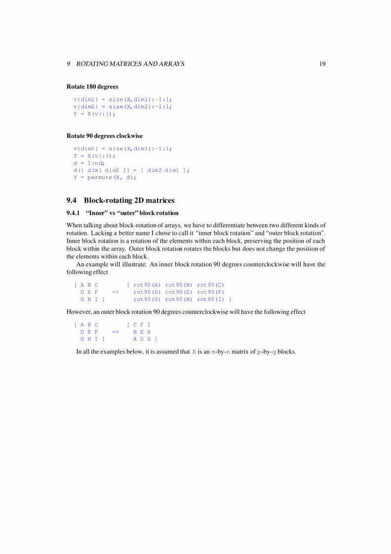
Rotate 180 degrees
v{dim1} = size(X,dim1):-1:1;
v{dim2} = size(X,dim2):-1:1;
Y = X(v{:});
Rotate 90 degrees clockwise
v{dim1} = size(X,dim1):-1:1;
Y = X(v{:});
d = 1:nd;
d([ dim1 dim2 ]) = [ dim2 dim1 ];
Y = permute(X, d);
9.4 Block-rotating 2D matrices
9.4.1 “Inner” vs “outer” block rotation
When talking about block-rotation of arrays, we have to differentiate between two different kinds of
rotation. Lacking a better name I chose to call it “inner block rotation” and “outer block rotation”.
Inner block rotation is a rotation of the elements within each block, preserving the position of each
block within the array. Outer block rotation rotates the blocks but does not change the position of
the elements within each block.
An example will illustrate: An inner block rotation 90 degrees counterclockwise will have the
following effect
[ A B C [ rot90(A) rot90(B) rot90(C)
D E F => rot90(D) rot90(E) rot90(F)G H I ] rot90(G) rot90(H) rot90(I) ]
However, an outer block rotation 90 degrees counterclockwise will have the following effect
[ A B C [ C F I
D E F => B E H
G H I ] A D G ]
In all the examples below, it is assumed that X is an m-by-n matrix of p-by-q blocks.
8/4/2019 Matlab Matrix and Array Operations
http://slidepdf.com/reader/full/matlab-matrix-and-array-operations 21/46
9 ROTATING MATRICES AND ARRAYS 20
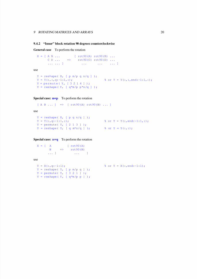
9.4.2 “Inner” block rotation 90 degrees counterclockwise
General case To perform the rotation
X = [ A B ... [ rot90(A) rot90(B) ...
C D ... => rot90(C) rot90(D) ...
... ... ] ... ... ... ]
use
Y = reshape( X, [ p m/p q n/q ] );
Y = Y(:,:,q:-1:1,:); % or Y = Y(:,:,end:-1:1,:);
Y = p e r m u t e ( Y , [ 3 2 1 4 ] ) ;
Y = reshape( Y, [ q*m/p p*n/q ] );
Special case: m=p To perform the rotation
[ A B ... ] => [ rot90(A) rot90(B) ... ]
use
Y = reshape( X, [ p q n/q ] );
Y = Y(:,q:-1:1,:); % or Y = Y(:,end:-1:1,:);
Y = permute( Y, [ 2 1 3 ] );
Y = reshape( Y, [ q m*n/q ] ); % or Y = Y(:,:);
Special case: n=q To perform the rotation
X = [ A [ rot90(A)B => rot90(B)
... ] ... ]
use
Y = X(:,q:-1:1); % or Y = X(:,end:-1:1);
Y = reshape( Y, [ p m/p q ] );
Y = permute( Y, [ 3 2 1 ] );
Y = reshape( Y, [ q*m/p p ] );
8/4/2019 Matlab Matrix and Array Operations
http://slidepdf.com/reader/full/matlab-matrix-and-array-operations 22/46
9 ROTATING MATRICES AND ARRAYS 21
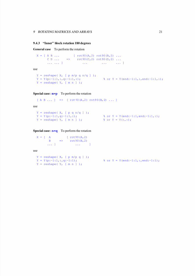
9.4.3 “Inner” block rotation 180 degrees
General case To perform the rotation
X = [ A B ... [ rot90(A,2) rot90(B,2) ...
C D ... => rot90(C,2) rot90(D,2) ...
... ... ] ... ... ... ]
use
Y = reshape( X, [ p m/p q n/q ] );
Y = Y(p:-1:1,:,q:-1:1,:); % or Y = Y(end:-1:1,:,end:-1:1,:);
Y = reshape( Y, [ m n ] );
Special case: m=p To perform the rotation
[ A B ... ] => [ rot90(A,2) rot90(B,2) ... ]
use
Y = reshape( X, [ p q n/q ] );
Y = Y(p:-1:1,q:-1:1,:); % or Y = Y(end:-1:1,end:-1:1,:);
Y = reshape( Y, [ m n ] ); % or Y = Y(:,:);
Special case: n=q To perform the rotation
X = [ A [ rot90(A,2)
B => rot90(B,2)
... ] ... ]
use
Y = reshape( X, [ p m/p q ] );
Y = Y(p:-1:1,:,q:-1:1); % or Y = Y(end:-1:1,:,end:-1:1);
Y = reshape( Y, [ m n ] );
8/4/2019 Matlab Matrix and Array Operations
http://slidepdf.com/reader/full/matlab-matrix-and-array-operations 23/46
9 ROTATING MATRICES AND ARRAYS 22
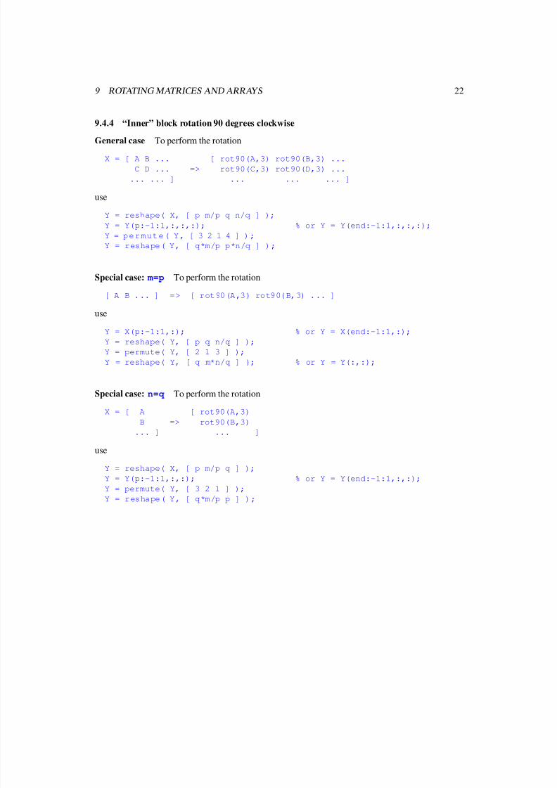
9.4.4 “Inner” block rotation 90 degrees clockwise
General case To perform the rotation
X = [ A B ... [ rot90(A,3) rot90(B,3) ...
C D ... => rot90(C,3) rot90(D,3) ...
... ... ] ... ... ... ]
use
Y = reshape( X, [ p m/p q n/q ] );
Y = Y(p:-1:1,:,:,:); % or Y = Y(end:-1:1,:,:,:);
Y = p e r m u t e ( Y , [ 3 2 1 4 ] ) ;
Y = reshape( Y, [ q*m/p p*n/q ] );
Special case: m=p To perform the rotation
[ A B ... ] => [ rot90(A,3) rot90(B,3) ... ]
use
Y = X(p:-1:1,:); % or Y = X(end:-1:1,:);
Y = reshape( Y, [ p q n/q ] );
Y = permute( Y, [ 2 1 3 ] );
Y = reshape( Y, [ q m*n/q ] ); % or Y = Y(:,:);
Special case: n=q To perform the rotation
X = [ A [ rot90(A,3)B => rot90(B,3)
... ] ... ]
use
Y = reshape( X, [ p m/p q ] );
Y = Y(p:-1:1,:,:); % or Y = Y(end:-1:1,:,:);
Y = permute( Y, [ 3 2 1 ] );
Y = reshape( Y, [ q*m/p p ] );
8/4/2019 Matlab Matrix and Array Operations
http://slidepdf.com/reader/full/matlab-matrix-and-array-operations 24/46
9 ROTATING MATRICES AND ARRAYS 23
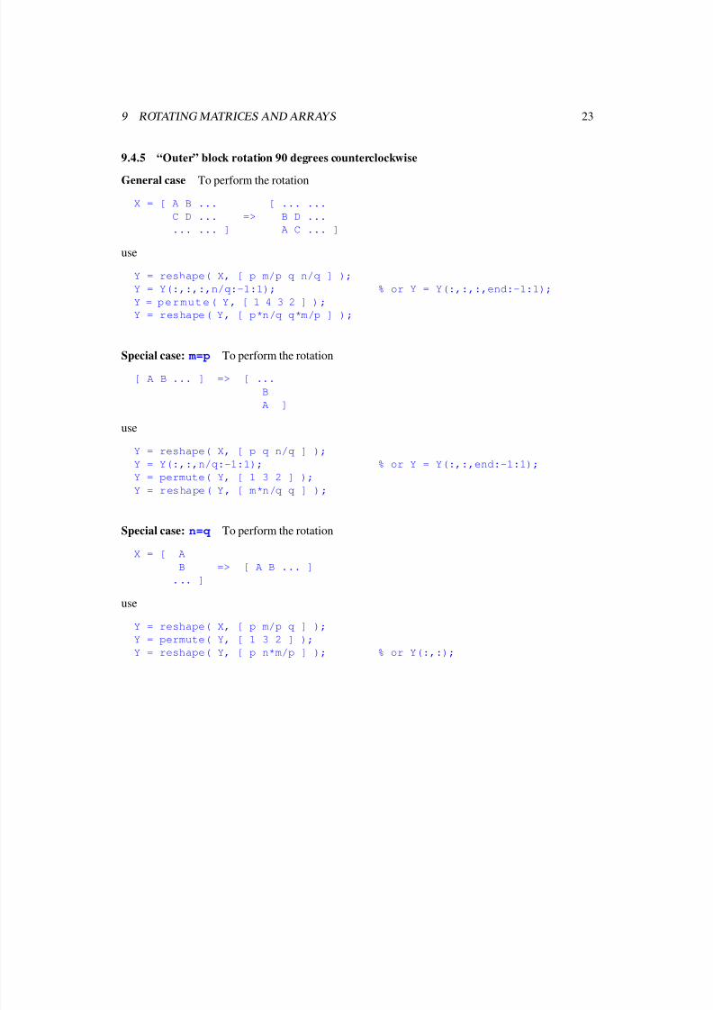
9.4.5 “Outer” block rotation 90 degrees counterclockwise
General case To perform the rotation
X = [ A B ... [ ... ...
C D ... => B D ...
... ... ] A C ... ]
use
Y = reshape( X, [ p m/p q n/q ] );
Y = Y(:,:,:,n/q:-1:1); % or Y = Y(:,:,:,end:-1:1);
Y = p e r m u t e ( Y , [ 1 4 3 2 ] ) ;
Y = reshape( Y, [ p*n/q q*m/p ] );
Special case: m=p To perform the rotation
[ A B ... ] => [ ...
B
A ]
use
Y = reshape( X, [ p q n/q ] );
Y = Y(:,:,n/q:-1:1); % or Y = Y(:,:,end:-1:1);
Y = permute( Y, [ 1 3 2 ] );
Y = reshape( Y, [ m*n/q q ] );
Special case: n=q To perform the rotation
X = [ A
B => [ A B ... ]
... ]
use
Y = reshape( X, [ p m/p q ] );
Y = permute( Y, [ 1 3 2 ] );
Y = reshape( Y, [ p n*m/p ] ); % or Y(:,:);
8/4/2019 Matlab Matrix and Array Operations
http://slidepdf.com/reader/full/matlab-matrix-and-array-operations 25/46
9 ROTATING MATRICES AND ARRAYS 24
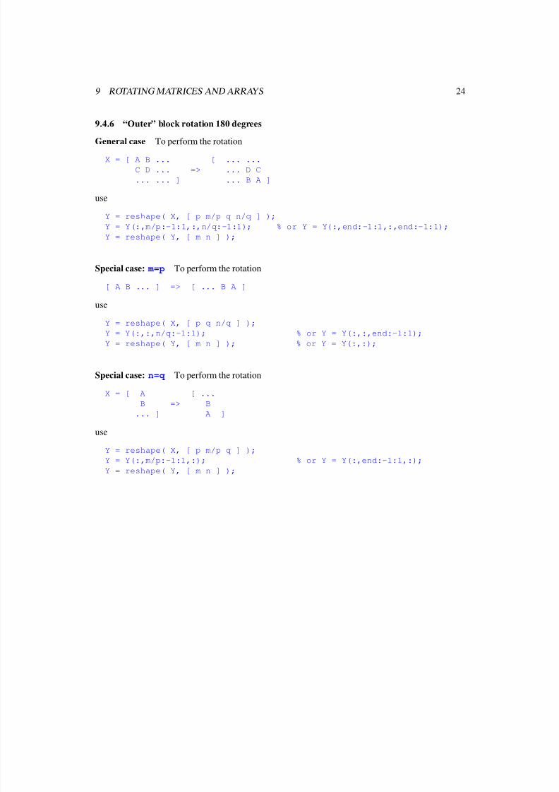
9.4.6 “Outer” block rotation 180 degrees
General case To perform the rotation
X = [ A B ... [ ... ...
C D ... => ... D C
... ... ] ... B A ]
use
Y = reshape( X, [ p m/p q n/q ] );
Y = Y(:,m/p:-1:1,:,n/q:-1:1); % or Y = Y(:,end:-1:1,:,end:-1:1);
Y = reshape( Y, [ m n ] );
Special case: m=p To perform the rotation
[ A B ... ] => [ ... B A ]
use
Y = reshape( X, [ p q n/q ] );
Y = Y(:,:,n/q:-1:1); % or Y = Y(:,:,end:-1:1);
Y = reshape( Y, [ m n ] ); % or Y = Y(:,:);
Special case: n=q To perform the rotation
X = [ A [ ...
B => B
... ] A ]
use
Y = reshape( X, [ p m/p q ] );
Y = Y(:,m/p:-1:1,:); % or Y = Y(:,end:-1:1,:);
Y = reshape( Y, [ m n ] );
8/4/2019 Matlab Matrix and Array Operations
http://slidepdf.com/reader/full/matlab-matrix-and-array-operations 26/46
9 ROTATING MATRICES AND ARRAYS 25
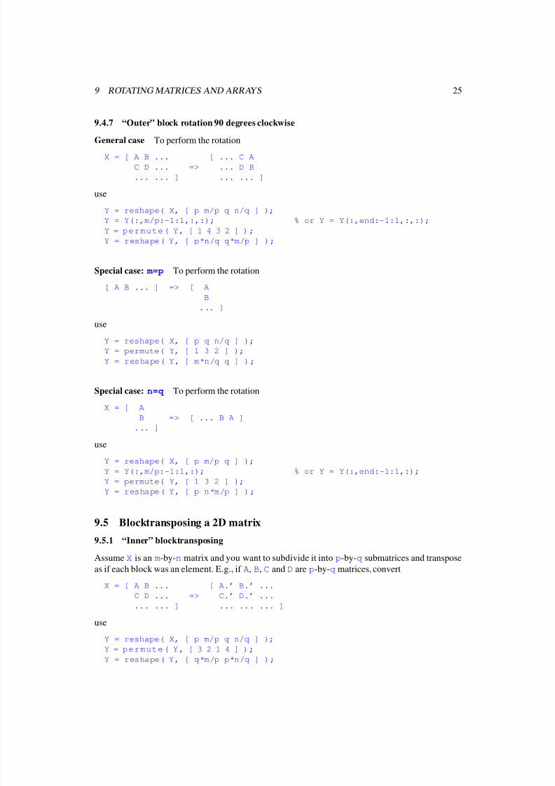
9.4.7 “Outer” block rotation 90 degrees clockwise
General case To perform the rotation
X = [ A B ... [ ... C A
C D ... => ... D B
... ... ] ... ... ]
use
Y = reshape( X, [ p m/p q n/q ] );
Y = Y(:,m/p:-1:1,:,:); % or Y = Y(:,end:-1:1,:,:);
Y = p e r m u t e ( Y , [ 1 4 3 2 ] ) ;
Y = reshape( Y, [ p*n/q q*m/p ] );
Special case: m=p To perform the rotation[ A B ... ] => [ A
B
... ]
use
Y = reshape( X, [ p q n/q ] );
Y = permute( Y, [ 1 3 2 ] );
Y = reshape( Y, [ m*n/q q ] );
Special case: n=q To perform the rotation
X = [ A
B => [ ... B A ]
... ]
use
Y = reshape( X, [ p m/p q ] );
Y = Y(:,m/p:-1:1,:); % or Y = Y(:,end:-1:1,:);
Y = permute( Y, [ 1 3 2 ] );
Y = reshape( Y, [ p n*m/p ] );
9.5 Blocktransposing a 2D matrix
9.5.1 “Inner” blocktransposing
Assume X is an m-by-n matrix and you want to subdivide it into p-by-q submatrices and transpose
as if each block was an element. E.g., if A, B, C and D are p-by-q matrices, convert
X = [ A B ... [ A.’ B.’ ...
C D ... => C.’ D.’ ...
... ... ] ... ... ... ]
use
Y = reshape( X, [ p m/p q n/q ] );
Y = p e r m u t e ( Y , [ 3 2 1 4 ] ) ;
Y = reshape( Y, [ q*m/p p*n/q ] );
8/4/2019 Matlab Matrix and Array Operations
http://slidepdf.com/reader/full/matlab-matrix-and-array-operations 27/46
10 MULTIPLY ARRAYS 26
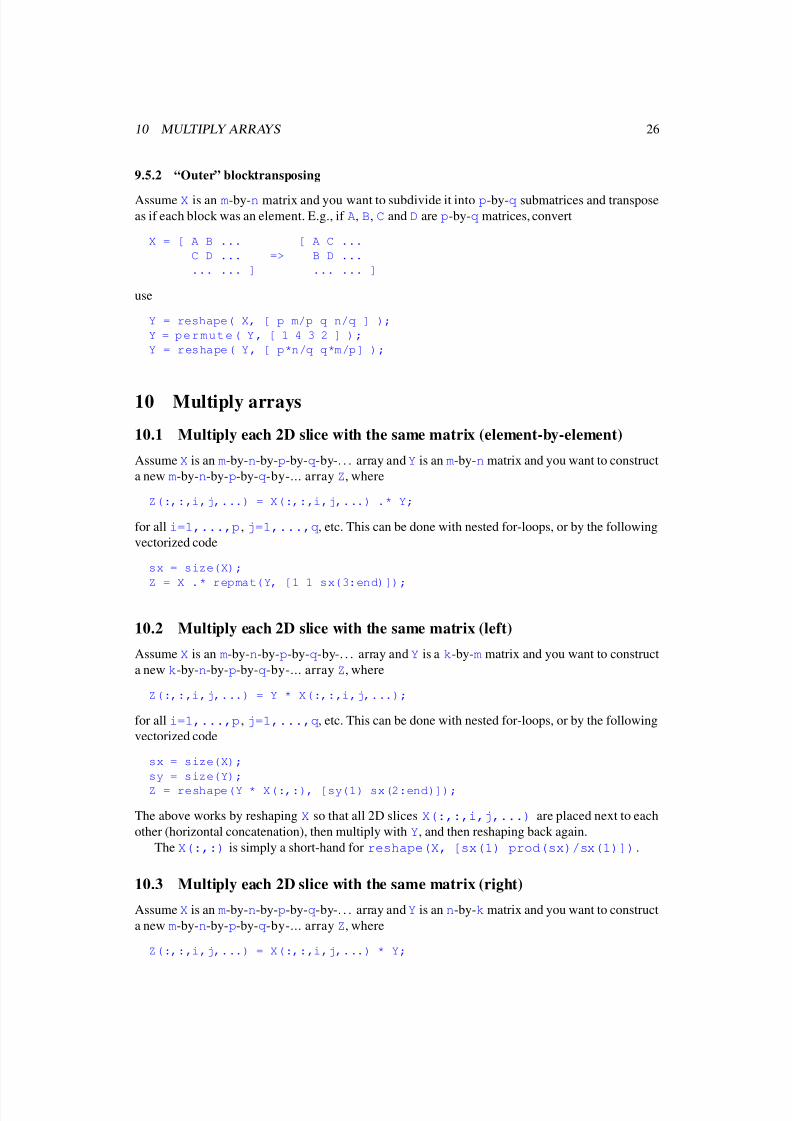
9.5.2 “Outer” blocktransposing
Assume X is an m-by-n matrix and you want to subdivide it into p-by-q submatrices and transposeas if each block was an element. E.g., if A, B, C and D are p-by-q matrices, convert
X = [ A B ... [ A C ...
C D ... => B D ...
... ... ] ... ... ]
use
Y = reshape( X, [ p m/p q n/q ] );
Y = p e r m u t e ( Y , [ 1 4 3 2 ] ) ;
Y = reshape( Y, [ p*n/q q*m/p] );
10 Multiply arrays
10.1 Multiply each 2D slice with the same matrix (element-by-element)
Assume X is an m-by-n-by-p-by-q-by-. . . array and Y is an m-by-n matrix and you want to construct
a new m-by-n-by-p-by-q-by-... array Z, where
Z(:,:,i,j,...) = X(:,:,i,j,...) .* Y;
for all i=1,...,p, j=1,...,q, etc. This can be done with nested for-loops, or by the following
vectorized code
sx = size(X);
Z = X .* repmat(Y, [1 1 sx(3:end)]);
10.2 Multiply each 2D slice with the same matrix (left)
Assume X is an m-by-n-by-p-by-q-by-. . . array and Y is a k-by-m matrix and you want to construct
a new k-by-n-by-p-by-q-by-... array Z, where
Z(:,:,i,j,...) = Y * X(:,:,i,j,...);
for all i=1,...,p, j=1,...,q, etc. This can be done with nested for-loops, or by the following
vectorized code
sx = size(X);
sy = size(Y);
Z = reshape(Y * X(:,:), [sy(1) sx(2:end)]);
The above works by reshaping X so that all 2D slices X(:,:,i,j,...) are placed next to each
other (horizontal concatenation), then multiply with Y, and then reshaping back again.
The X(:,:) is simply a short-hand for reshape(X, [sx(1) prod(sx)/sx(1)]).
10.3 Multiply each 2D slice with the same matrix (right)
Assume X is an m-by-n-by-p-by-q-by-. . . array and Y is an n-by-k matrix and you want to construct
a new m-by-n-by-p-by-q-by-... array Z, where
Z(:,:,i,j,...) = X(:,:,i,j,...) * Y;
8/4/2019 Matlab Matrix and Array Operations
http://slidepdf.com/reader/full/matlab-matrix-and-array-operations 28/46
10 MULTIPLY ARRAYS 27
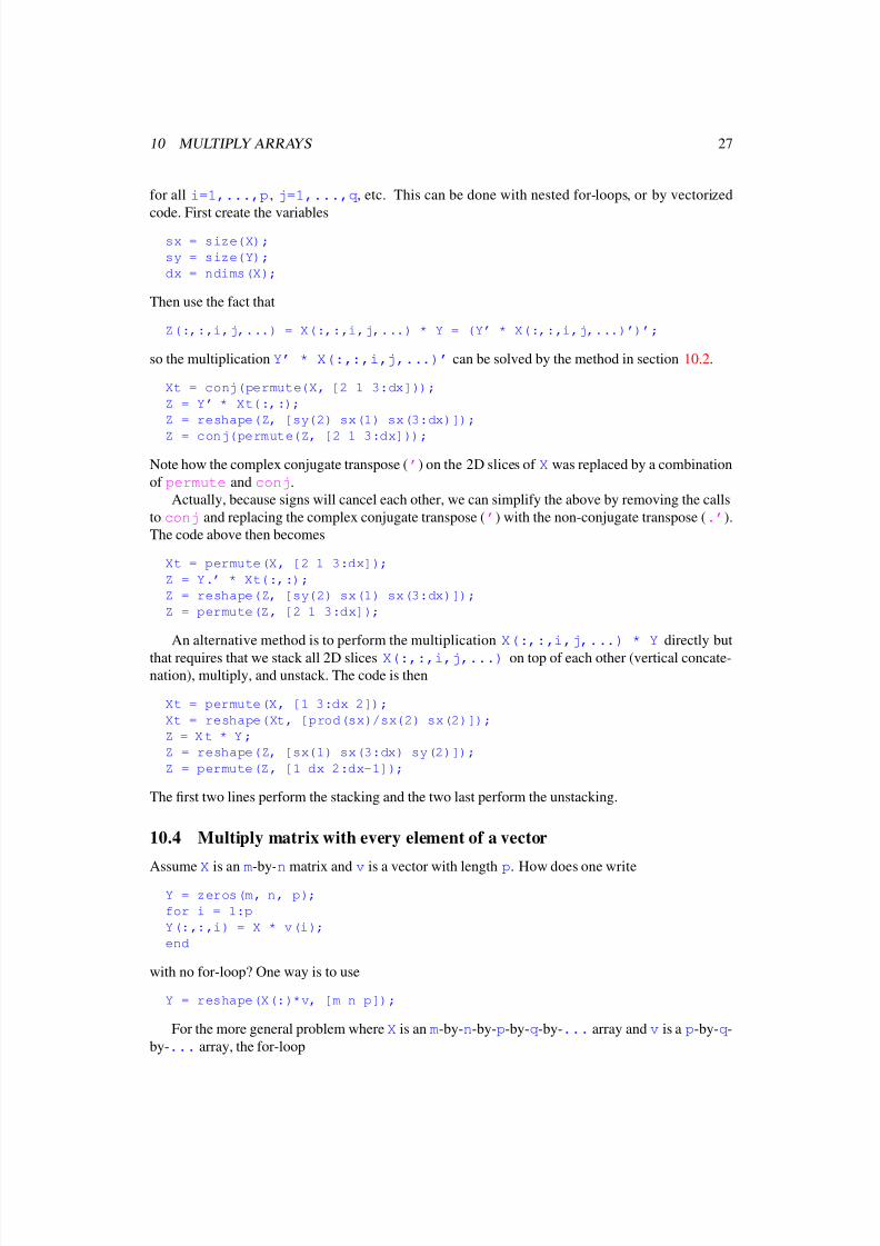
for all i=1,...,p, j=1,...,q, etc. This can be done with nested for-loops, or by vectorized
code. First create the variablessx = size(X);
sy = size(Y);
dx = ndims(X);
Then use the fact that
Z(:,:,i,j,...) = X(:,:,i,j,...) * Y = (Y’ * X(:,:,i,j,...)’)’;
so the multiplication Y’ * X(:,:,i,j,...)’ can be solved by the method in section 10.2.
Xt = conj(permute(X, [2 1 3:dx]));
Z = Y’ * Xt(:,:);
Z = reshape(Z, [sy(2) sx(1) sx(3:dx)]);
Z = conj(permute(Z, [2 1 3:dx]));
Note how the complex conjugate transpose (’) on the 2D slices of X was replaced by a combination
of permute and conj.
Actually, because signs will cancel each other, we can simplify the above by removing the calls
to conj and replacing the complex conjugate transpose (’) with the non-conjugate transpose (.’).
The code above then becomes
Xt = permute(X, [2 1 3:dx]);
Z = Y.’ * Xt(:,:);
Z = reshape(Z, [sy(2) sx(1) sx(3:dx)]);
Z = permute(Z, [2 1 3:dx]);
An alternative method is to perform the multiplication X(:,:,i,j,...) * Y directly but
that requires that we stack all 2D slices X(:,:,i,j,...) on top of each other (vertical concate-nation), multiply, and unstack. The code is then
Xt = permute(X, [1 3:dx 2]);
Xt = reshape(Xt, [prod(sx)/sx(2) sx(2)]);
Z = X t * Y ;
Z = reshape(Z, [sx(1) sx(3:dx) sy(2)]);
Z = permute(Z, [1 dx 2:dx-1]);
The first two lines perform the stacking and the two last perform the unstacking.
10.4 Multiply matrix with every element of a vector
Assume X is an m-by-n matrix and v is a vector with length p. How does one writeY = zeros(m, n, p);
for i = 1:p
Y(:,:,i) = X * v(i);
end
with no for-loop? One way is to use
Y = reshape(X(:)*v, [m n p]);
For the more general problem where X is an m-by-n-by-p-by-q-by-... array and v is a p-by-q-
by-... array, the for-loop
8/4/2019 Matlab Matrix and Array Operations
http://slidepdf.com/reader/full/matlab-matrix-and-array-operations 29/46
10 MULTIPLY ARRAYS 28
Y = zeros(m, n, p, q, ...);
...
for j = 1:q
for i = 1:p
Y(:,:,i,j,...) = X(:,:,i,j,...) * v(i,j,...);
end
end
...
may be written as
sx = size(X);
Z = X .* repmat(reshape(v, [1 1 sx(3:end)]), [sx(1) sx(2)]);
10.5 Multiply each 2D slice with corresponding element of a vectorAssume X is an m-by-n-by-p array and v is a row vector with length p. How does one write
Y = zeros(m, n, p);
for i = 1:p
Y(:,:,i) = X(:,:,i) * v(i);
end
with no for-loop? One way is to use
Y = X .* repmat(reshape(v, [1 1 p]), [m n]);
10.6 Outer product of all rows in a matrixAssume X is an m-by-n matrix. How does one create an n-by-n-by-m matrix Y so that, for all i from
1 to m,
Y(:,:,i) = X(i,:)’ * X(i,:);
The obvious for-loop solution is
Y = zeros(n, n, m);
for i = 1:m
Y(:,:,i) = X(i,:)’ * X(i,:);
end
a non-for-loop solution is
j = 1:n;
Y = reshape(repmat(X’, n, 1) .* X(:,j(ones(n, 1),:)).’, [n n m]);
Note the use of the non-conjugate transpose in the second factor to ensure that it works correctly
also for complex matrices.
10.7 Keeping only diagonal elements of multiplication
Assume X and Y are two m-by-n matrices and that W is an n-by-n matrix. How does one vectorize
the following for-loop
8/4/2019 Matlab Matrix and Array Operations
http://slidepdf.com/reader/full/matlab-matrix-and-array-operations 30/46
11 DIVIDE ARRAYS 29
Z = zeros(m, 1);
for i = 1:m
Z(i) = X(i,:)*W*Y(i,:)’;
end
Two solutions are
Z = diag(X*W*Y’); % (1)
Z = sum(X*W.*conj(Y), 2); % (2)
Solution (1) does a lot of unnecessary work, since we only keep the n diagonal elements of the nˆ2
computed elements. Solution (2) only computes the elements of interest and is significantly faster if
n is large.
10.8 Products involving the Kronecker product
The following is based on a posting by Paul Fackler <[email protected]> to the Usenet newsgroup comp.soft-sys.matlab.
Kronecker products of the form kron(A, eye(n)) are often used to premultiply (or post-
multiply) another matrix. If this is the case it is not necessary to actually compute and store the
Kronecker product. Assume A is an p-by-q matrix and that B is a q*n-by-m matrix.
Then the following two p*n-by-m matrices are identical
C1 = kron(A, eye(n))*B;
C2 = reshape(reshape(B.’, [n*m q])*A.’, [m p*n]).’;
The following two p*n-by-m matrices are also identical.
C1 = kron(eye(n), A)*B;
C2 = reshape(A*reshape(B, [q n*m]), [p*n m]);
11 Divide arrays
11.1 Divide each 2D slice with the same matrix (element-by-element)
Assume X is an m-by-n-by-p-by-q-by-. . . array and Y is an m-by-n matrix and you want to construct
a new m-by-n-by-p-by-q-by-... array Z, where
Z(:,:,i,j,...) = X(:,:,i,j,...) ./ Y;
for all i=1,...,p, j=1,...,q, etc. This can be done with nested for-loops, or by the following
vectorized code
sx = size(X);
Z = X./repmat(Y, [1 1 sx(3:end)]);
11.2 Divide each 2D slice with the same matrix (left)
Assume X is an m-by-n-by-p-by-q-by-. . . array and Y is an m-by-m matrix and you want to construct
a new m-by-n-by-p-by-q-by-... array Z, where
Z(:,:,i,j,...) = Y \ X(:,:,i,j,...);
for all i=1,...,p, j=1,...,q, etc. This can be done with nested for-loops, or by the following
vectorized code
Z = reshape(Y\X(:,:), size(X));
8/4/2019 Matlab Matrix and Array Operations
http://slidepdf.com/reader/full/matlab-matrix-and-array-operations 31/46
12 CALCULATING DISTANCES 30
11.3 Divide each 2D slice with the same matrix (right)
Assume X is an m-by-n-by-p-by-q-by-. . . array and Y is an m-by-m matrix and you want to constructa new m-by-n-by-p-by-q-by-... array Z, where
Z(:,:,i,j,...) = X(:,:,i,j,...) / Y;
for all i=1,...,p, j=1,...,q, etc. This can be done with nested for-loops, or by the following
vectorized code
sx = size(X);
dx = ndims(X);
Xt = reshape(permute(X, [1 3:dx 2]), [prod(sx)/sx(2) sx(2)]);
Z = Xt/Y;
Z = permute(reshape(Z, sx([1 3:dx 2])), [1 dx 2:dx-1]);
The third line above builds a 2D matrix which is a vertical concatenation (stacking) of all 2D slicesX(:,:,i,j,...). The fourth line does the actual division. The fifth line does the opposite of the
third line.
The five lines above might be simplified a little by introducing a dimension permutation vector
sx = size(X);
dx = ndims(X);
v = [1 3:dx 2];
Xt = reshape(permute(X, v), [prod(sx)/sx(2) sx(2)]);
Z = Xt/Y;
Z = ipermute(reshape(Z, sx(v)), v);
If you don’t care about readability, this code may also be written as
sx = size(X);dx = ndims(X);
v = [1 3:dx 2];
Z = ipermute(reshape(reshape(permute(X, v), ...
[prod(sx)/sx(2) sx(2)])/Y, sx(v)), v);
12 Calculating distances
12.1 Euclidean distance
The Euclidean distance from xi to y j is
di j = xi−y j =
( x1i− y1 j)2 + · · ·+ ( x pi− y p j)2
12.2 Distance between two points
To calculate the Euclidean distance from a point represented by the vector x to another point repre-
seted by the vector y, use one of
d = norm(x-y);
d = sqrt(sum(abs(x-y).^2));
8/4/2019 Matlab Matrix and Array Operations
http://slidepdf.com/reader/full/matlab-matrix-and-array-operations 32/46
12 CALCULATING DISTANCES 31
12.3 Euclidean distance vector
Assume X is an m-by-p matrix representing m points in p-dimensional space and y is a 1-by-p vectorrepresenting a single point in the same space. Then, to compute the m-by-1 distance vector d where
d(i) is the Euclidean distance between X(i,:) and y, use
d = sqrt(sum(abs(X - repmat(y, [m 1])).^2, 2));
d = sqrt(sum(abs(X - y(ones(m,1),:)).^2, 2)); % inline call to repmat
12.4 Euclidean distance matrix
Assume X is an m-by-p matrix representing m points in p-dimensional space and Y is an n-by-p
matrix representing another set of points in the same space. Then, to compute the m-by-n distance
matrix D where D(i,j) is the Euclidean distance X(i,:) between Y(j,:), use
D = sqrt(sum(abs( repmat(permute(X, [1 3 2]), [1 n 1]) ...
- repmat(permute(Y, [3 1 2]), [m 1 1]) ).^2, 3));
The following code inlines the call to repmat, but requires to temporary variables unless one do-
esn’t mind changing X and Y
Xt = permute(X, [1 3 2]);
Yt = permute(Y, [3 1 2]);
D = sqrt(sum(abs( Xt(:,ones(1,n),:) ...
- Yt(ones(1,m),:,:) ).^2, 3));
The distance matrix may also be calculated without the use of a 3-D array:
i = (1:m).’; % index vector for x
i = i(:,ones(1,n)); % index matrix for x
j = 1:n; % index vector for y
j = j(ones(1,m),:); % index matrix for y
D = zeros(m, n); % initialise output matrix
D(:) = sqrt(sum(abs(X(i(:),:) - Y(j(:),:)).^2, 2));
12.5 Special case when both matrices are identical
If X and Y are identical one may use the following, which is nothing but a rewrite of the code above
D = sqrt(sum(abs( repmat(permute(X, [1 3 2]), [1 m 1]) ...
- repmat(permute(X, [3 1 2]), [m 1 1]) ).^2, 3));
One might want to take advantage of the fact that D will be symmetric. The following code firstcreates the indices for the upper triangular part of D. Then it computes the upper triangular part of D
and finally lets the lower triangular part of D be a mirror image of the upper triangular part.
[ i j ] = find(triu(ones(m), 1)); % trick to get indices
D = zeros(m, m); % initialise output matrix
D( i + m*(j-1) ) = sqrt(sum(abs( X(i,:) - X(j,:) ).^2, 2));
D( j + m*(i-1) ) = D( i + m*(j-1) );
8/4/2019 Matlab Matrix and Array Operations
http://slidepdf.com/reader/full/matlab-matrix-and-array-operations 33/46
12 CALCULATING DISTANCES 32
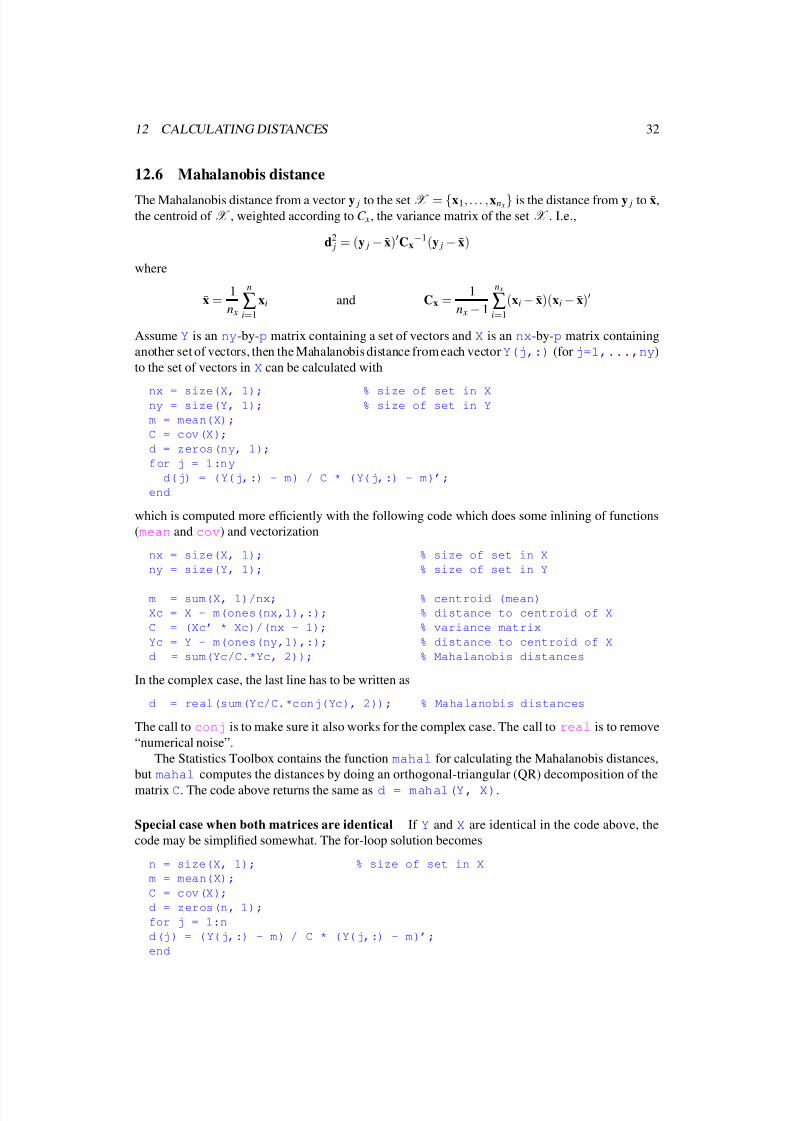
12.6 Mahalanobis distance
The Mahalanobis distance from a vector y j to the set X = {x1, . . . , xn x} is the distance from y j to x̄,the centroid of X , weighted according to C x, the variance matrix of the set X . I.e.,
d2 j = (y j− x̄)Cx
−1(y j− x̄)
where
x̄ =1
n x
n
∑i=1
xi and Cx =1
n x−1
n x
∑i=1
(xi− x̄)(xi− x̄)
Assume Y is an ny-by-p matrix containing a set of vectors and X is an nx-by-p matrix containing
another set of vectors, then the Mahalanobis distance from each vector Y(j,:) (for j=1,...,ny)
to the set of vectors in X can be calculated with
nx = size(X, 1); % size of set in Xny = size(Y, 1); % size of set in Y
m = mean(X);
C = cov(X);
d = zeros(ny, 1);
for j = 1:ny
d(j) = (Y(j,:) - m) / C * (Y(j,:) - m)’;
end
which is computed more efficiently with the following code which does some inlining of functions
(mean and cov) and vectorization
nx = size(X, 1); % size of set in X
ny = size(Y, 1); % size of set in Y
m = sum(X, 1)/nx; % centroid (mean)
Xc = X - m(ones(nx,1),:); % distance to centroid of X
C = (Xc’ * Xc)/(nx - 1); % variance matrix
Yc = Y - m(ones(ny,1),:); % distance to centroid of X
d = sum(Yc/C.*Yc, 2)); % Mahalanobis distances
In the complex case, the last line has to be written as
d = real(sum(Yc/C.*conj(Yc), 2)); % Mahalanobis distances
The call to conj is to make sure it also works for the complex case. The call to real is to remove
“numerical noise”.
The Statistics Toolbox contains the function mahal for calculating the Mahalanobis distances,
but mahal computes the distances by doing an orthogonal-triangular (QR) decomposition of the
matrix C. The code above returns the same as d = mahal(Y, X).
Special case when both matrices are identical If Y and X are identical in the code above, the
code may be simplified somewhat. The for-loop solution becomes
n = size(X, 1); % size of set in X
m = mean(X);
C = cov(X);
d = zeros(n, 1);
for j = 1:n
d(j) = (Y(j,:) - m) / C * (Y(j,:) - m)’;
end
8/4/2019 Matlab Matrix and Array Operations
http://slidepdf.com/reader/full/matlab-matrix-and-array-operations 34/46
13 STATISTICS, PROBABILITY AND COMBINATORICS 33
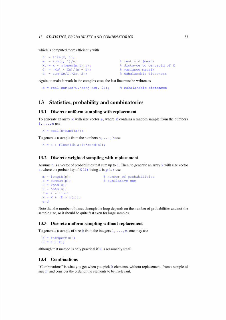
which is computed more efficiently with
n = size(x, 1);
m = sum(x, 1)/n; % centroid (mean)
Xc = x - m(ones(n,1),:); % distance to centroid of X
C = (Xc’ * Xc)/(n - 1); % variance matrix
d = sum(Xc/C.*Xc, 2); % Mahalanobis distances
Again, to make it work in the complex case, the last line must be written as
d = real(sum(Xc/C.*conj(Xc), 2)); % Mahalanobis distances
13 Statistics, probability and combinatorics
13.1 Discrete uniform sampling with replacementTo generate an array X with size vector s, where X contains a random sample from the numbers
1,...,n use
X = ceil(n*rand(s));
To generate a sample from the numbers a,...,b use
X = a + floor((b-a+1)*rand(s));
13.2 Discrete weighted sampling with replacement
Assume p is a vector of probabilities that sum up to 1. Then, to generate an array X with size vector
s, where the probability of X(i) being i is p(i) use
m = length(p); % number of probabilities
c = cumsum(p); % cumulative sum
R = rand(s);
X = ones(s);
for i = 1:m-1
X = X + (R > c(i));
end
Note that the number of times through the loop depends on the number of probabilities and not the
sample size, so it should be quite fast even for large samples.
13.3 Discrete uniform sampling without replacementTo generate a sample of size k from the integers 1,...,n, one may use
X = randperm(n);
x = X(1:k);
although that method is only practical if N is reasonably small.
13.4 Combinations
“Combinations” is what you get when you pick k elements, without replacement, from a sample of
size n, and consider the order of the elements to be irrelevant.
8/4/2019 Matlab Matrix and Array Operations
http://slidepdf.com/reader/full/matlab-matrix-and-array-operations 35/46
13 STATISTICS, PROBABILITY AND COMBINATORICS 34
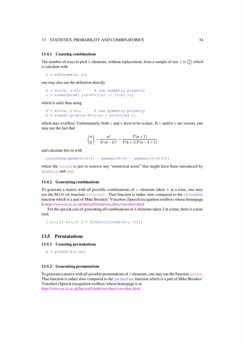
13.4.1 Counting combinations
The number of ways to pick k elements, without replacement, from a sample of size n isnk
which
is calculate with
c = nchoosek(n, k);
one may also use the definition directly
k = min(k, n-k); % use symmetry property
c = round(prod( ((n-k+1):n) ./ (1:k) ));
which is safer than using
k = min(k, n-k); % use symmetry property
c = round( prod((n-k+1):n) / prod(1:k) );
which may overflow. Unfortunately, both n and k have to be scalars. If n and/or k are vectors, one
may use the fact that
n
k
=
n!
k ! (n− k )!=
Γ (n + 1)
Γ (k + 1)Γ (n− k + 1)
and calculate this in with
round(exp(gammaln(n+1) - gammaln(k+1) - gammaln(n-k+1)))
where the round is just to remove any “numerical noise” that might have been introduced by
gammaln and exp.
13.4.2 Generating combinations
To generate a matrix with all possible combinations of n elements taken k at a time, one may
use the MATLAB function nchoosek. That function is rather slow compared to the choosenk
function which is a part of Mike Brookes’ Voicebox (Speech recognition toolbox) whose homepage
is http://www.ee.ic.ac.uk/hp/staff/dmb/voicebox/voicebox.html
For the special case of generating all combinations of n elements taken 2 at a time, there is a neat
trick
[ x(:,2) x(:,1) ] = find(tril(ones(n), -1));
13.5 Permutations
13.5.1 Counting permutations
p = prod(n-k+1:n);
13.5.2 Generating permutations
To generate a matrix with all possible permutations of n elements, one may use the function perms.
That function is rather slow compared to the permutes function which is a part of Mike Brookes’
Voicebox (Speech recognition toolbox) whose homepage is at
http://www.ee.ic.ac.uk/hp/staff/dmb/voicebox/voicebox.html
8/4/2019 Matlab Matrix and Array Operations
http://slidepdf.com/reader/full/matlab-matrix-and-array-operations 36/46
14 TYPES OF ARRAYS 35
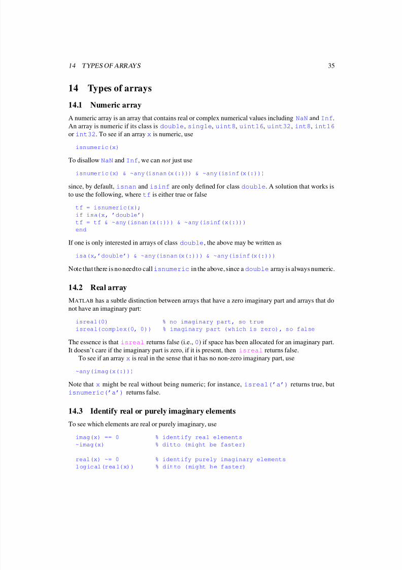
14 Types of arrays
14.1 Numeric array
A numeric array is an array that contains real or complex numerical values including NaN and Inf.
An array is numeric if its class is double, single, uint8, uint16, uint32, int8, int16
or int32. To see if an array x is numeric, use
isnumeric(x)
To disallow NaN and Inf, we can not just use
isnumeric(x) & ~any(isnan(x(:))) & ~any(isinf(x(:)))
since, by default, isnan and isinf are only defined for class double. A solution that works is
to use the following, where tf is either true or false
tf = isnumeric(x);
if isa(x, ’double’)
tf = tf & ~any(isnan(x(:))) & ~any(isinf(x(:)))
end
If one is only interested in arrays of class double, the above may be written as
isa(x,’double’) & ~any(isnan(x(:))) & ~any(isinf(x(:)))
Note that there is no needto call isnumeric in the above, since a double array is always numeric.
14.2 Real array
MATLAB has a subtle distinction between arrays that have a zero imaginary part and arrays that donot have an imaginary part:
isreal(0) % no imaginary part, so true
isreal(complex(0, 0)) % imaginary part (which is zero), so false
The essence is that isreal returns false (i.e., 0) if space has been allocated for an imaginary part.
It doesn’t care if the imaginary part is zero, if it is present, then isreal returns false.
To see if an array x is real in the sense that it has no non-zero imaginary part, use
~any(imag(x(:)))
Note that x might be real without being numeric; for instance, isreal(’a’) returns true, but
isnumeric(’a’) returns false.
14.3 Identify real or purely imaginary elements
To see which elements are real or purely imaginary, use
imag(x) == 0 % identify real elements
~imag(x) % ditto (might be faster)
real(x) ~= 0 % identify purely imaginary elements
logical(real(x)) % ditto (might be faster)
8/4/2019 Matlab Matrix and Array Operations
http://slidepdf.com/reader/full/matlab-matrix-and-array-operations 37/46
14 TYPES OF ARRAYS 36
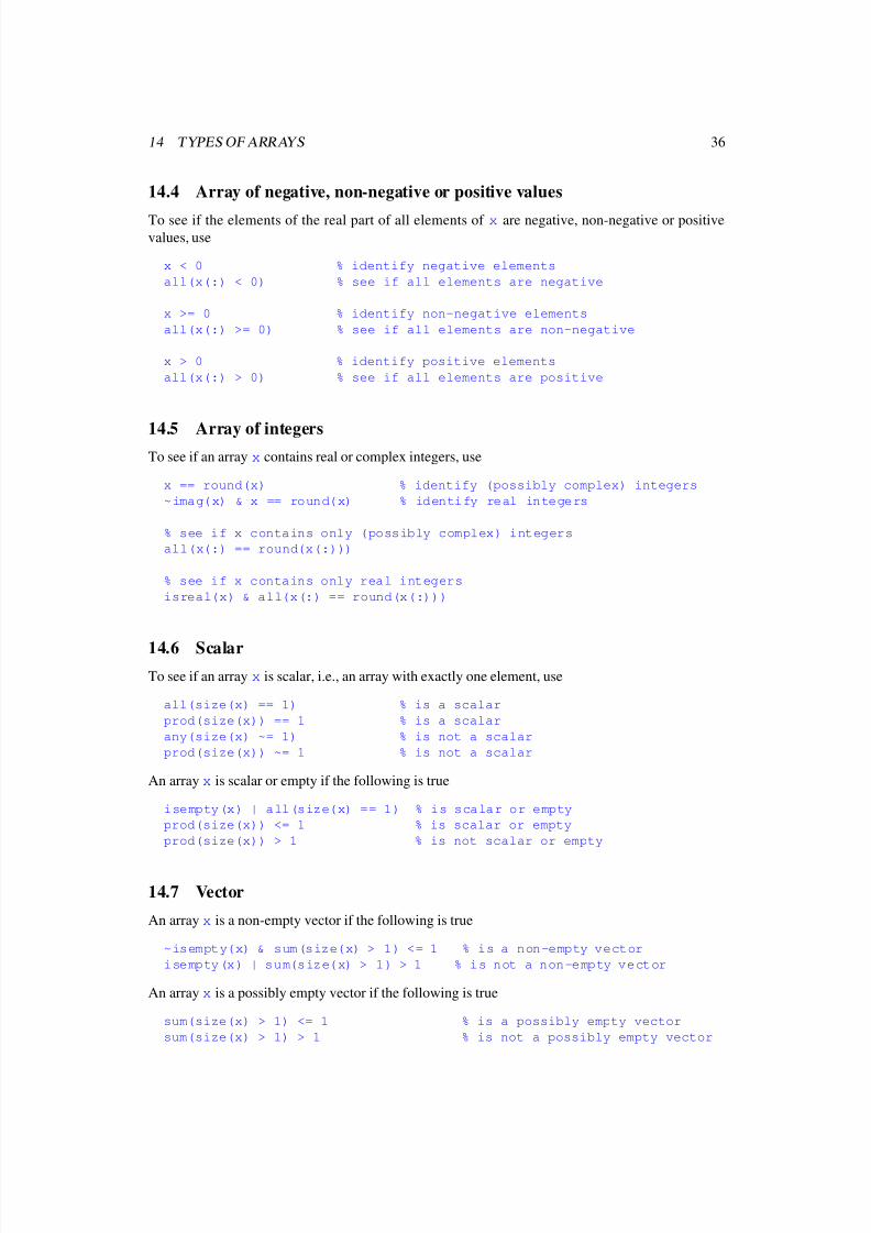
14.4 Array of negative, non-negative or positive values
To see if the elements of the real part of all elements of x are negative, non-negative or positivevalues, use
x < 0 % identify negative elements
all(x(:) < 0) % see if all elements are negative
x >= 0 % identify non-negative elements
all(x(:) >= 0) % see if all elements are non-negative
x > 0 % identify positive elements
all(x(:) > 0) % see if all elements are positive
14.5 Array of integersTo see if an array x contains real or complex integers, use
x == round(x) % identify (possibly complex) integers
~imag(x) & x == round(x) % identify real integers
% see if x contains only (possibly complex) integers
all(x(:) == round(x(:)))
% see if x contains only real integers
isreal(x) & all(x(:) == round(x(:)))
14.6 Scalar
To see if an array x is scalar, i.e., an array with exactly one element, use
all(size(x) == 1) % is a scalar
prod(size(x)) == 1 % is a scalar
any(size(x) ~= 1) % is not a scalar
prod(size(x)) ~= 1 % is not a scalar
An array x is scalar or empty if the following is true
isempty(x) | all(size(x) == 1) % is scalar or empty
prod(size(x)) <= 1 % is scalar or empty
prod(size(x)) > 1 % is not scalar or empty
14.7 Vector
An array x is a non-empty vector if the following is true
~isempty(x) & sum(size(x) > 1) <= 1 % is a non-empty vector
isempty(x) | sum(size(x) > 1) > 1 % is not a non-empty vector
An array x is a possibly empty vector if the following is true
sum(size(x) > 1) <= 1 % is a possibly empty vector
sum(size(x) > 1) > 1 % is not a possibly empty vector
8/4/2019 Matlab Matrix and Array Operations
http://slidepdf.com/reader/full/matlab-matrix-and-array-operations 38/46
15 LOGICAL OPERATORS AND COMPARISONS 37
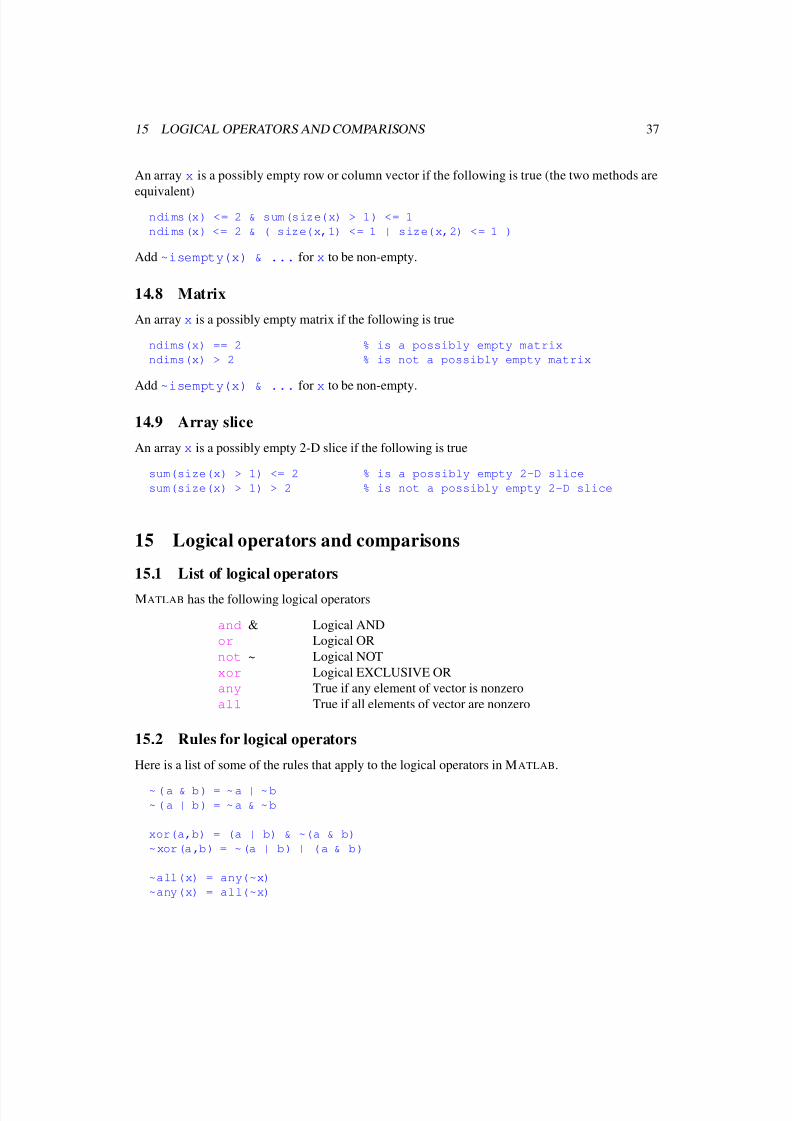
An array x is a possibly empty row or column vector if the following is true (the two methods are
equivalent)ndims(x) <= 2 & sum(size(x) > 1) <= 1
ndims(x) <= 2 & ( size(x,1) <= 1 | size(x,2) <= 1 )
Add ~isempty(x) & ... for x to be non-empty.
14.8 Matrix
An array x is a possibly empty matrix if the following is true
ndims(x) == 2 % is a possibly empty matrix
ndims(x) > 2 % is not a possibly empty matrix
Add ~isempty(x) & ... for x to be non-empty.
14.9 Array slice
An array x is a possibly empty 2-D slice if the following is true
sum(size(x) > 1) <= 2 % is a possibly empty 2-D slice
sum(size(x) > 1) > 2 % is not a possibly empty 2-D slice
15 Logical operators and comparisons
15.1 List of logical operators
MATLAB has the following logical operators
and & Logical AND
or Logical OR
not ~ Logical NOT
xor Logical EXCLUSIVE OR
any True if any element of vector is nonzero
all True if all elements of vector are nonzero
15.2 Rules for logical operators
Here is a list of some of the rules that apply to the logical operators in MATLAB.
~ ( a & b ) = ~ a | ~ b
~ ( a | b ) = ~ a & ~ b
xor(a,b) = (a | b) & ~(a & b)
~xor(a,b) = ~(a | b) | (a & b)
~all(x) = any(~x)
~any(x) = all(~x)
8/4/2019 Matlab Matrix and Array Operations
http://slidepdf.com/reader/full/matlab-matrix-and-array-operations 39/46
16 MISCELLANEOUS 38
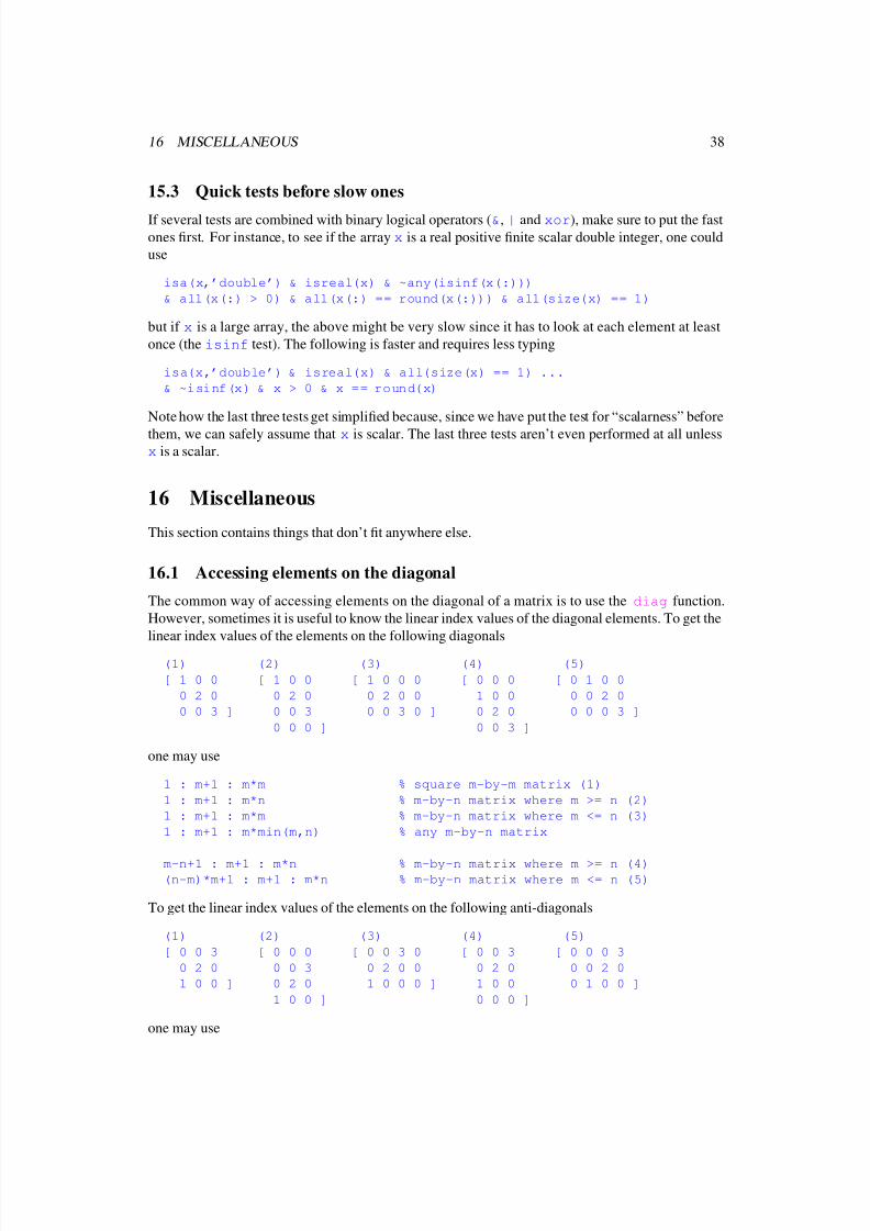
15.3 Quick tests before slow ones
If several tests are combined with binary logical operators (&, | and xor), make sure to put the fastones first. For instance, to see if the array x is a real positive finite scalar double integer, one could
use
isa(x,’double’) & isreal(x) & ~any(isinf(x(:)))
& all(x(:) > 0) & all(x(:) == round(x(:))) & all(size(x) == 1)
but if x is a large array, the above might be very slow since it has to look at each element at least
once (the isinf test). The following is faster and requires less typing
isa(x,’double’) & isreal(x) & all(size(x) == 1) ...
& ~isinf(x) & x > 0 & x == round(x)
Note how the last three tests get simplified because, since we have put the test for “scalarness” before
them, we can safely assume that x is scalar. The last three tests aren’t even performed at all unlessx is a scalar.
16 Miscellaneous
This section contains things that don’t fit anywhere else.
16.1 Accessing elements on the diagonal
The common way of accessing elements on the diagonal of a matrix is to use the diag function.
However, sometimes it is useful to know the linear index values of the diagonal elements. To get the
linear index values of the elements on the following diagonals
(1) (2) (3) (4) (5)
[ 1 0 0 [ 1 0 0 [ 1 0 0 0 [ 0 0 0 [ 0 1 0 0
0 2 0 0 2 0 0 2 0 0 1 0 0 0 0 2 0
0 0 3 ] 0 0 3 0 0 3 0 ] 0 2 0 0 0 0 3 ]
0 0 0 ] 0 0 3 ]
one may use
1 : m+1 : m*m % square m-by-m matrix (1)
1 : m+1 : m*n % m-by-n matrix where m >= n (2)
1 : m+1 : m*m % m-by-n matrix where m <= n (3)
1 : m+1 : m*min(m,n) % any m-by-n matrix
m-n+1 : m+1 : m*n % m-by-n matrix where m >= n (4)(n-m)*m+1 : m+1 : m*n % m-by-n matrix where m <= n (5)
To get the linear index values of the elements on the following anti-diagonals
(1) (2) (3) (4) (5)
[ 0 0 3 [ 0 0 0 [ 0 0 3 0 [ 0 0 3 [ 0 0 0 3
0 2 0 0 0 3 0 2 0 0 0 2 0 0 0 2 0
1 0 0 ] 0 2 0 1 0 0 0 ] 1 0 0 0 1 0 0 ]
1 0 0 ] 0 0 0 ]
one may use
8/4/2019 Matlab Matrix and Array Operations
http://slidepdf.com/reader/full/matlab-matrix-and-array-operations 40/46
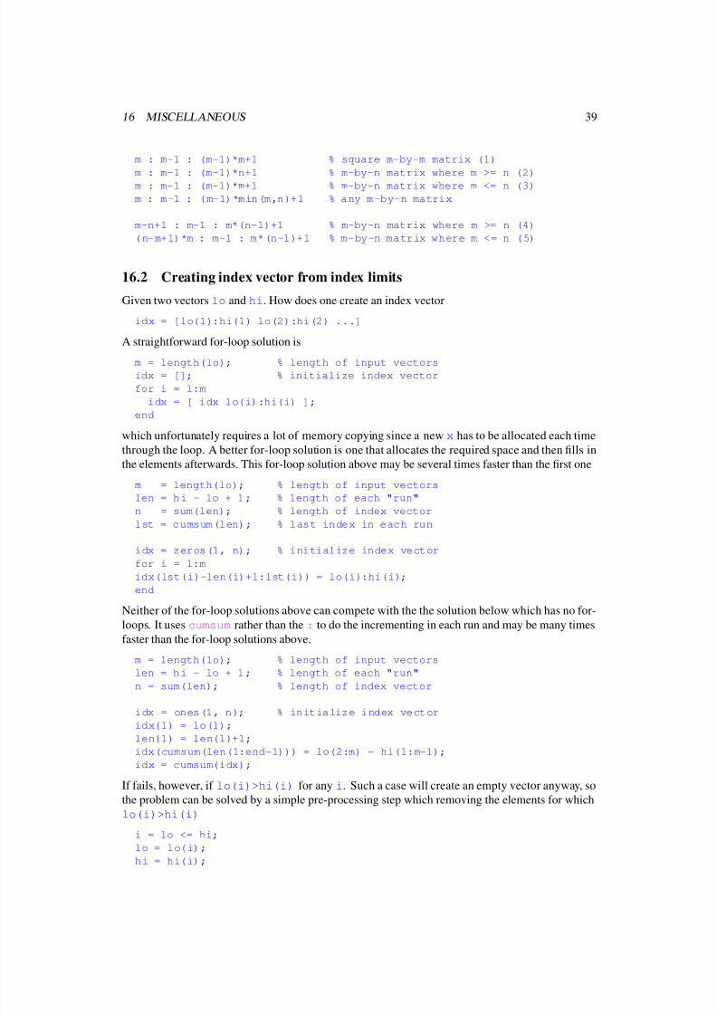
16 MISCELLANEOUS 39
m : m-1 : (m-1)*m+1 % square m-by-m matrix (1)
m : m-1 : (m-1)*n+1 % m-by-n matrix where m >= n (2)
m : m-1 : (m-1)*m+1 % m-by-n matrix where m <= n (3)
m : m-1 : (m-1)*min(m,n)+1 % any m-by-n matrix
m-n+1 : m-1 : m*(n-1)+1 % m-by-n matrix where m >= n (4)
(n-m+1)*m : m-1 : m*(n-1)+1 % m-by-n matrix where m <= n (5)
16.2 Creating index vector from index limits
Given two vectors lo and hi. How does one create an index vector
idx = [lo(1):hi(1) lo(2):hi(2) ...]
A straightforward for-loop solution is
m = length(lo); % length of input vectors
idx = []; % initialize index vector
for i = 1:m
idx = [ idx lo(i):hi(i) ];
end
which unfortunately requires a lot of memory copying since a new x has to be allocated each time
through the loop. A better for-loop solution is one that allocates the required space and then fills in
the elements afterwards. This for-loop solution above may be several times faster than the first one
m = length(lo); % length of input vectors
len = h i - lo + 1 ; % length of each "run"
n = sum(len); % length of index vector
lst = cumsum(len); % last index in each run
idx = zeros(1, n); % initialize index vector
for i = 1:m
idx(lst(i)-len(i)+1:lst(i)) = lo(i):hi(i);
end
Neither of the for-loop solutions above can compete with the the solution below which has no for-
loops. It uses cumsum rather than the : to do the incrementing in each run and may be many times
faster than the for-loop solutions above.
m = length(lo); % length of input vectors
len = h i - lo + 1 ; % length of each "run"
n = sum(len); % length of index vector
idx = ones(1, n); % initialize index vectoridx(1) = lo(1);
len(1) = len(1)+1;
idx(cumsum(len(1:end-1))) = lo(2:m) - hi(1:m-1);
idx = cumsum(idx);
If fails, however, if lo(i)>hi(i) for any i. Such a case will create an empty vector anyway, so
the problem can be solved by a simple pre-processing step which removing the elements for which
lo(i)>hi(i)
i = lo <= hi;
lo = lo(i);
hi = hi(i);
8/4/2019 Matlab Matrix and Array Operations
http://slidepdf.com/reader/full/matlab-matrix-and-array-operations 41/46
16 MISCELLANEOUS 40
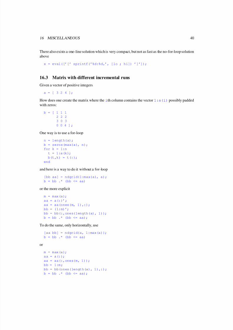
There also exists a one-line solution which is very compact, but not as fast as the no-for-loop solution
abovex = eval([’[’ sprintf(’%d:%d,’, [lo ; hi]) ’]’]);
16.3 Matrix with different incremental runs
Given a vector of positive integers
a = [ 3 2 4 ];
How does one create the matrix where the ith column contains the vector 1:a(i) possibly padded
with zeros:
b = [ 1 1 1
2 2 2
3 0 3
0 0 4 ] ;
One way is to use a for-loop
n = length(a);
b = zeros(max(a), n);
for k = 1:n
t = 1:a(k);
b(t,k) = t(:);
end
and here is a way to do it without a for-loop
[bb aa] = ndgrid(1:max(a), a);
b = bb .* (bb <= aa)
or the more explicit
m = max(a);
aa = a(:)’;
aa = aa(ones(m, 1),:);
bb = (1:m)’;
bb = bb(:,ones(length(a), 1));
b = bb .* (bb <= aa);
To do the same, only horizontally, use
[aa bb] = ndgrid(a, 1:max(a));
b = bb .* (bb <= aa)
or
m = max(a);
aa = a(:);
aa = aa(:,ones(m, 1));
bb = 1:m;
bb = bb(ones(length(a), 1),:);
b = bb .* (bb <= aa);
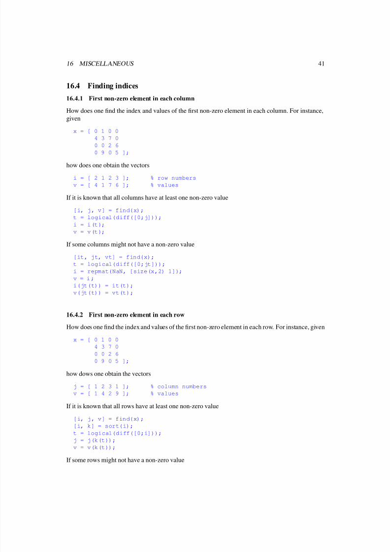
8/4/2019 Matlab Matrix and Array Operations
http://slidepdf.com/reader/full/matlab-matrix-and-array-operations 42/46
16 MISCELLANEOUS 41
16.4 Finding indices
16.4.1 First non-zero element in each column
How does one find the index and values of the first non-zero element in each column. For instance,
given
x = [ 0 1 0 0
4 3 7 0
0 0 2 6
0 9 0 5 ];
how does one obtain the vectors
i = [ 2 1 2 3 ]; % row numbers
v = [ 4 1 7 6 ]; % values
If it is known that all columns have at least one non-zero value
[i, j, v] = find(x);
t = logical(diff([0;j]));
i = i(t);
v = v(t);
If some columns might not have a non-zero value
[it, jt, vt] = find(x);
t = logical(diff([0;jt]));
i = repmat(NaN, [size(x,2) 1]);
v = i ;
i(jt(t)) = it(t);
v(jt(t)) = vt(t);
16.4.2 First non-zero element in each row
How does one find the index and values of the first non-zero element in each row. For instance, given
x = [ 0 1 0 0
4 3 7 0
0 0 2 6
0 9 0 5 ];
how dows one obtain the vectors
j = [ 1 2 3 1 ]; % column numbersv = [ 1 4 2 9 ]; % values
If it is known that all rows have at least one non-zero value
[i, j, v] = find(x);
[i, k] = sort(i);
t = logical(diff([0;i]));
j = j(k(t));
v = v(k(t));
If some rows might not have a non-zero value
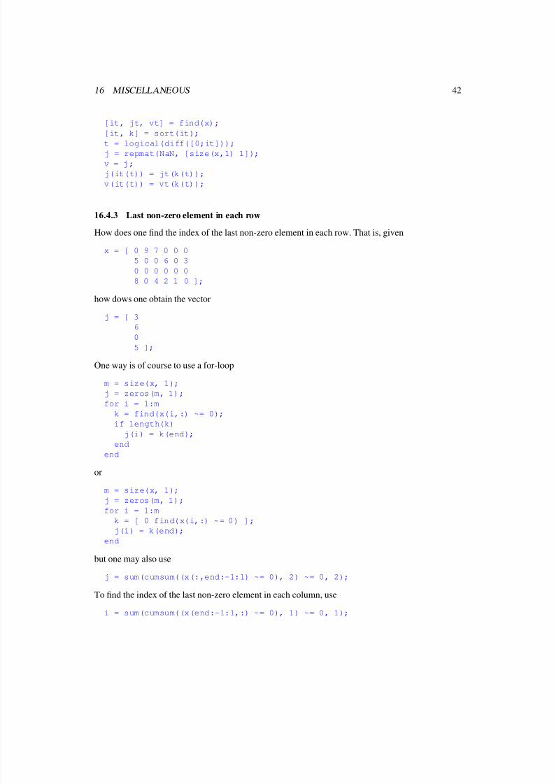
8/4/2019 Matlab Matrix and Array Operations
http://slidepdf.com/reader/full/matlab-matrix-and-array-operations 43/46
16 MISCELLANEOUS 42
[it, jt, vt] = find(x);
[it, k] = sort(it);
t = logical(diff([0;it]));
j = repmat(NaN, [size(x,1) 1]);
v = j ;
j(it(t)) = jt(k(t));
v(it(t)) = vt(k(t));
16.4.3 Last non-zero element in each row
How does one find the index of the last non-zero element in each row. That is, given
x = [ 0 9 7 0 0 0
5 0 0 6 0 3
0 0 0 0 0 08 0 4 2 1 0 ];
how dows one obtain the vector
j = [ 3
6
0
5 ];
One way is of course to use a for-loop
m = size(x, 1);
j = zeros(m, 1);
for i = 1:m
k = find(x(i,:) ~= 0);if length(k)
j(i) = k(end);
end
end
or
m = size(x, 1);
j = zeros(m, 1);
for i = 1:m
k = [ 0 find(x(i,:) ~= 0) ];
j(i) = k(end);
end
but one may also use
j = sum(cumsum((x(:,end:-1:1) ~= 0), 2) ~= 0, 2);
To find the index of the last non-zero element in each column, use
i = sum(cumsum((x(end:-1:1,:) ~= 0), 1) ~= 0, 1);
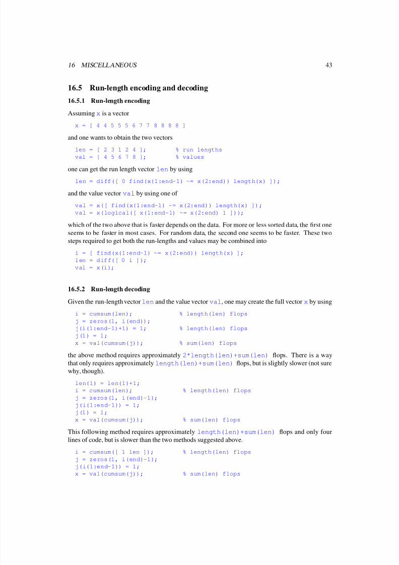
8/4/2019 Matlab Matrix and Array Operations
http://slidepdf.com/reader/full/matlab-matrix-and-array-operations 44/46
16 MISCELLANEOUS 43
16.5 Run-length encoding and decoding
16.5.1 Run-length encoding
Assuming x is a vector
x = [ 4 4 5 5 5 6 7 7 8 8 8 8 ]
and one wants to obtain the two vectors
len = [ 2 3 1 2 4 ]; % run lengths
val = [ 4 5 6 7 8 ]; % values
one can get the run length vector len by using
len = diff([ 0 find(x(1:end-1) ~= x(2:end)) length(x) ]);
and the value vector val by using one of
val = x([ find(x(1:end-1) ~= x(2:end)) length(x) ]);
val = x(logical([ x(1:end-1) ~= x(2:end) 1 ]));
which of the two above that is faster depends on the data. For more or less sorted data, the first one
seems to be faster in most cases. For random data, the second one seems to be faster. These two
steps required to get both the run-lengths and values may be combined into
i = [ find(x(1:end-1) ~= x(2:end)) length(x) ];
len = diff([ 0 i ]);
val = x(i);
16.5.2 Run-length decoding
Given the run-length vector len and the value vector val, one may create the full vector x by using
i = cumsum(len); % length(len) flops
j = zeros(1, i(end));
j(i(1:end-1)+1) = 1; % length(len) flops
j(1) = 1;
x = val(cumsum(j)); % sum(len) flops
the above method requires approximately 2*length(len)+sum(len) flops. There is a way
that only requires approximately length(len)+sum(len) flops, but is slightly slower (not sure
why, though).
len(1) = len(1)+1;
i = cumsum(len); % length(len) flops
j = zeros(1, i(end)-1);
j(i(1:end-1)) = 1;
j(1) = 1;
x = val(cumsum(j)); % sum(len) flops
This following method requires approximately length(len)+sum(len) flops and only four
lines of code, but is slower than the two methods suggested above.
i = cumsum([ 1 len ]); % length(len) flops
j = zeros(1, i(end)-1);
j(i(1:end-1)) = 1;
x = val(cumsum(j)); % sum(len) flops
8/4/2019 Matlab Matrix and Array Operations
http://slidepdf.com/reader/full/matlab-matrix-and-array-operations 45/46
16 MISCELLANEOUS 44
16.6 Counting bits
Assume x is an array of non-negative integers. The number of set bits in each element, nsetbits,is
nsetbits = reshape(sum(dec2bin(x)-’0’, 2), size(x));
or
bin = dec2bin(x);
nsetbits = reshape(sum(bin,2) - ’0’*size(bin,2), size(x));
The following solution is slower, but requires less memory than the above so it is able to handle
larger arrays
nsetbits = zeros(size(x));
k = find(x);while length(k)
nsetbits = nsetbits + bitand(x, 1);
x = bitshift(x, -1);
k = k(logical(x(k)));
end
The total number of set bits, nsetbits, may be computed with
bin = dec2bin(x);
nsetbits = sum(bin(:)) - ’0’*prod(size(bin));
nsetbits = 0;
k = find(x);
while length(k)
nsetbits = nsetbits + sum(bitand(x, 1));
x = bitshift(x, -1);
k = k(logical(x(k)));
end
Glossary
null-operation an operation which has no effect on the operand
operand an argument on which an operator is applied
singleton dimension a dimension along which the length is zero
subscript context an expression used as an array subscript is in a subscript context
vectorization taking advantage of the fact that many operators and functions can perform the same
operation on several elements in an array without requiring the use of a for-loop
8/4/2019 Matlab Matrix and Array Operations
http://slidepdf.com/reader/full/matlab-matrix-and-array-operations 46/46
Indexmatlab faq, 5
comp.soft-sys.matlab, 4, 5
dimensions
number of, 9
singleton, 9
trailing singleton, 9
elements
number of, 9
null-operation, 9
run-length
decoding, 43
encoding, 43
shift
elements in vectors, 11
singleton dimensions, see dimensions, single-
ton
size, 8
trailing singleton dimensions, see dimensions,trailing singleton
Usenet, 4
vectorization, 5