mathematics of seismic imaging part i - mathtube.org · mathematics of seismic imaging part i...
TRANSCRIPT

Mathematics of Seismic ImagingPart I
William W. Symes
PIMS, July 2005

A mathematical view
...of reflection seismic imaging, as practiced in the petroleum industry:
• an inverse problem, based on a model of seismic wave propagation
• contemporary practice relies onpartial linearizationand high-frequency asymp-totics
• recent progress in understanding capabilities, limitations of methods based onlinearization/asymptotics in presence ofstrong refraction: applications ofmi-crolocal analysiswith implications for practice
• limitations of linearization lead to many open problems
1

Agenda
1. The reflection seismic experiment, nature of data and of Earth mechanical fields,the acoustic model, linearization and its limitations, definition of imaging basedon high frequency asymptotics, geometric optics analysis of the model-data rela-tionship and the GRT representation, zero-offset migration, standard processing= layered imaging
2. Analysis of GRT migration, asymptotic inversion, difficulties due to multipathing,global theory of imaging, ”wave equation” imaging;
3. The partially linearized inverse problem (“velocity analysis”), extended models,importance of invertibility, geometric optics of extensions, some invertible ex-tensions, automating the solution of the partially linearized inverse problem viadifferential semblance.
2

Marine reflection seismology
• acoustic source (airgun array, explosives,...)
• acoustic receivers (hydrophone streamer, ocean bottom cable,...)
• recording and onboard processing
hydrophone streameracoustic source(airgun array)x xr sh
Land acquisition similar, but acquisition and processing are more complex. Vastbulk (90%+) of data acquired each year is marine.
Data parameters: timet, source locationxs, and receiver locationxr or half offseth = xr−xs
2 , h = |h|.
3

Idealized marine “streamer” geometry:xs andxr lie roughly on constant depthplane, source-receiver lines are parallel→ 3 spatial degrees of freedom (eg.xs, h):codimension 1. [Other geometries are interesting, eg. ocean bottom cables, butstreamer surveys still prevalent.]
How much data? Contemporary surveys may feature
• Simultaneous recording by multiple streamers (up to 12!)
• Many (roughly) parallel ship tracks (“lines”), areal coverage
• single line (“2D”)∼ Gbyte; multiple lines (“3D”)∼ Tbyte
NB: In these lectures, will largely ignore sampling issues and treat data as contin-uously sampled.First of many approximations...
4

Gathers: distinguished data subsets
Aka “bins”, extracted from data after acquisition.
Characterized by common value of an acquisition parameter
• shot (or common source) gather: traces with same shot location xs (previousexpls)
• offset (or common offset) gather: traces with same half offset h
• ...
5

Shot gather, Mississippi Canyon
0
1
2
3
4
5
time
(s)
-4 -3 -2 -1offset (km)
(thanks: Exxon)
6
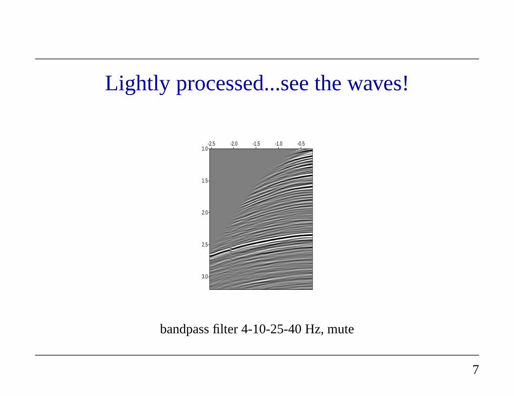
Lightly processed...see the waves!
1.0
1.5
2.0
2.5
3.0
-2.5 -2.0 -1.5 -1.0 -0.5
bandpass filter 4-10-25-40 Hz, mute
7

A key observation
The most striking visual characteristic of seismic reflection data: presence of waveevents (“reflections”) = coherent space-time structures.
What features in the subsurface structure cause reflectionsto occur?
Abrupt (wavelength scale) changes in material mechanics act as internal bound-aries, causing reflection of waves.
What is the mechanism through which this occurs?
8

Well logs: a “direct” view of the subsurface
1000 1200 1400 1600 1800 2000 2200 2400 2600 2800 3000500
1000
1500
2000
2500
3000
3500
4000
4500
depth (m)
Blocked logs from well in North Sea (thanks: Mobil R & D). Solid: p-wave ve-locity (m/s), dashed: s-wave velocity (m/s), dash-dot: density (kg/m3). “Blocked”means “averaged” (over 30 m windows). Original sample rate of log tool < 1 m.Reflectors= jumps in velocities, density,velocity trends.
9

The Modeling Task
A useful model of the reflection seismology experiment must
• predict wave motion
• produce reflections from reflectors
• accomodate significant variation of wave velocity, material density,...
A really goodmodel will also accomodate
• multiple wave modes, speeds
• material anisotropy
• attenuation, frequency dispersion of waves
• complex source, receiver characteristics
10

The Acoustic Model
Not really good, but good enough for this week and basis of most contemporaryprocessing.
Relatesρ(x)= material density,λ(x) = bulk modulus,p(x, t)= pressure,v(x, t) =particle velocity,f(x, t)= force density (sound source):
ρ∂v
∂t= −∇p + f ,
∂p
∂t= −λ∇ · v (+ i.c.′s, b.c.′s)
(compressional) wave speedc =√
λρ
11

acoustic field potentialu(x, t) =∫ t
−∞ ds p(x, s):
p =∂u
∂t, v =
1
ρ∇u
Equivalent form: second order wave equation for potential
1
ρc2
∂2u
∂t2−∇ ·
1
ρ∇u =
∫ t
−∞
dt∇ ·
(
f
ρ
)
≡f
ρ
plus initial, boundary conditions.
12

Theory
Weak solutionof Dirichlet problem inΩ ⊂ R3 (similar treatment for other b. c.’s):
u ∈ C1([0, T ]; L2(Ω)) ∩ C0([0, T ]; H10(Ω))
satisfying for anyφ ∈ C∞0 ((0, T ) × Ω),
∫ T
0
∫
Ω
dt dx
1
ρc2
∂u
∂t
∂φ
∂t−
1
ρ∇u · ∇φ +
1
ρfφ
= 0
Theorem (Lions, 1972) Suppose thatlog ρ, log c ∈ L∞(Ω), f ∈ L2(Ω × R). Thenweak solutions of Dirichlet problem exist, uniquely determined by initial data
u(·, 0) ∈ H10(Ω),
∂u
∂t(·, 0) ∈ L2(Ω)
NB: No hint of waves here...
13
Further idealizations
• density is constant,
• source force density isisotropic point radiator with known time dependence(“source pulse”w(t))
f(x, t;xs) = w(t)δ(x− xs)
⇒ acoustic potential, pressure depends onxs also.
Forward map F [c] = time history of pressure for eachxs at receiver locationsxr
(predicted seismic data), as function of velocity fieldc(x):
F [c] = p(xr, t;xs)
14

Reflection seismic inverse problem
givenobserved seismic datad, find c so that
F [c] ≃ d
This inverse problem is
• large scale - up to Tbytes, Pflops
• nonlinear
• yields to no known direct attack
15

Partial linearization
Almost all useful technology to date relies on partial linearization: writec = v(1+r)
and treatr as relative first order perturbation aboutv, resulting in perturbation ofpresure fieldδp = ∂δu
∂t= 0, t ≤ 0, where
(
1
v2
∂2
∂t2−∇2
)
δu =2r
v2
∂2u
∂t2
Definelinearized forward map F by
F [v]r = δp(xr, t;xs)
Analysis ofF [v] is the main content of contemporary reflection seismic theory.
16

Linearization error
Critical question: If there is any justiceF [v]r = directional derivativeDF [v][vr]
of F - but in what sense? Physical intuition, numerical simulation, and not nearlyenough mathematics: linearization error
F [v(1 + r)] − (F [v] + F [v]r)
• smallwhenv smooth,r rough or oscillatory on wavelength scale - well-separatedscales
• largewhenv not smooth and/orr not oscillatory - poorly separated scales
2D finite difference simulation: shot gathers with typical marine seismic geometry.Smooth (linear)v(x, z), oscillatory (random)r(x, z) depending only onz(“layeredmedium”). Source waveletw(t) = bandpass filter.
17
0
0.2
0.4
0.6
0.8
1.0
z (k
m)
0 0.5 1.0 1.5 2.0x (km)
1.6
1.8
2.0
2.2
2.4
,
0
0.2
0.4
0.6
0.8
t (s)
0 0.2 0.4 0.6 0.8 1.0x_r (km)
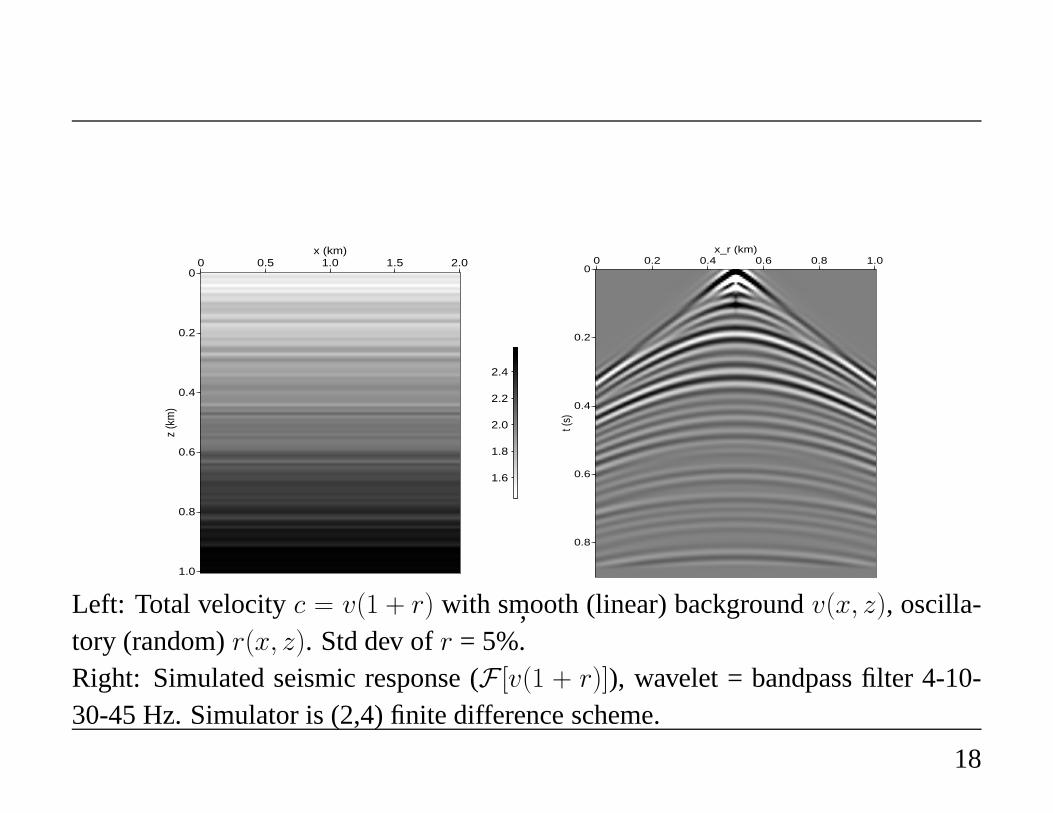
Left: Total velocityc = v(1 + r) with smooth (linear) backgroundv(x, z), oscilla-tory (random)r(x, z). Std dev ofr = 5%.Right: Simulated seismic response (F [v(1 + r)]), wavelet = bandpass filter 4-10-30-45 Hz. Simulator is (2,4) finite difference scheme.
18

0
0.2
0.4
0.6
0.8
1.0
z (k
m)
0 0.5 1.0 1.5 2.0x (km)
1.6
1.8
2.0
2.2
2.4
,
0
0.2
0.4
0.6
0.8
1.0z
(km
)
0 0.5 1.0 1.5 2.0x (km)
-0.10
-0.05
0
0.05
0.10
Model in previous slide as smooth background (left,v(x, z)) plus rough perturba-tion (right,r(x, z)).
19

0
0.2
0.4
0.6
0.8
t (s)
0 0.2 0.4 0.6 0.8 1.0x_r (km)
.
0
0.2
0.4
0.6
0.8
t (s)
0 0.2 0.4 0.6 0.8 1.0x_r (km)
Left: Simulated seismic response of smooth model (F [v]),Right: Simulated linearized response, rough perturbationof smooth model (F [v]r)
20
0
0.2
0.4
0.6
0.8
1.0
z (k
m)
0 0.5 1.0 1.5 2.0x (km)
1.4
1.6
1.8
2.0
2.2
2.4
,
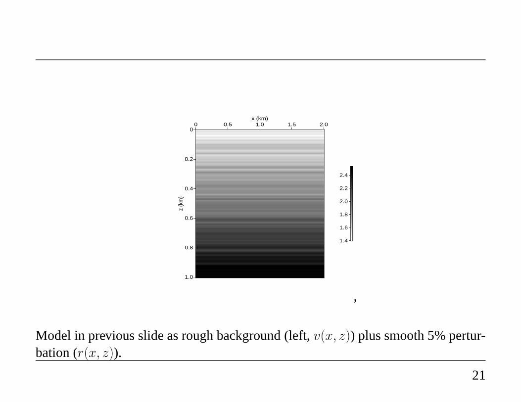
Model in previous slide as rough background (left,v(x, z)) plus smooth 5% pertur-bation (r(x, z)).
21
0
0.2
0.4
0.6
0.8
t (s)
0 0.2 0.4 0.6 0.8 1.0x_r (km)
.
0
0.2
0.4
0.6
0.8
t (s)
0 0.2 0.4 0.6 0.8 1.0x_r (km)
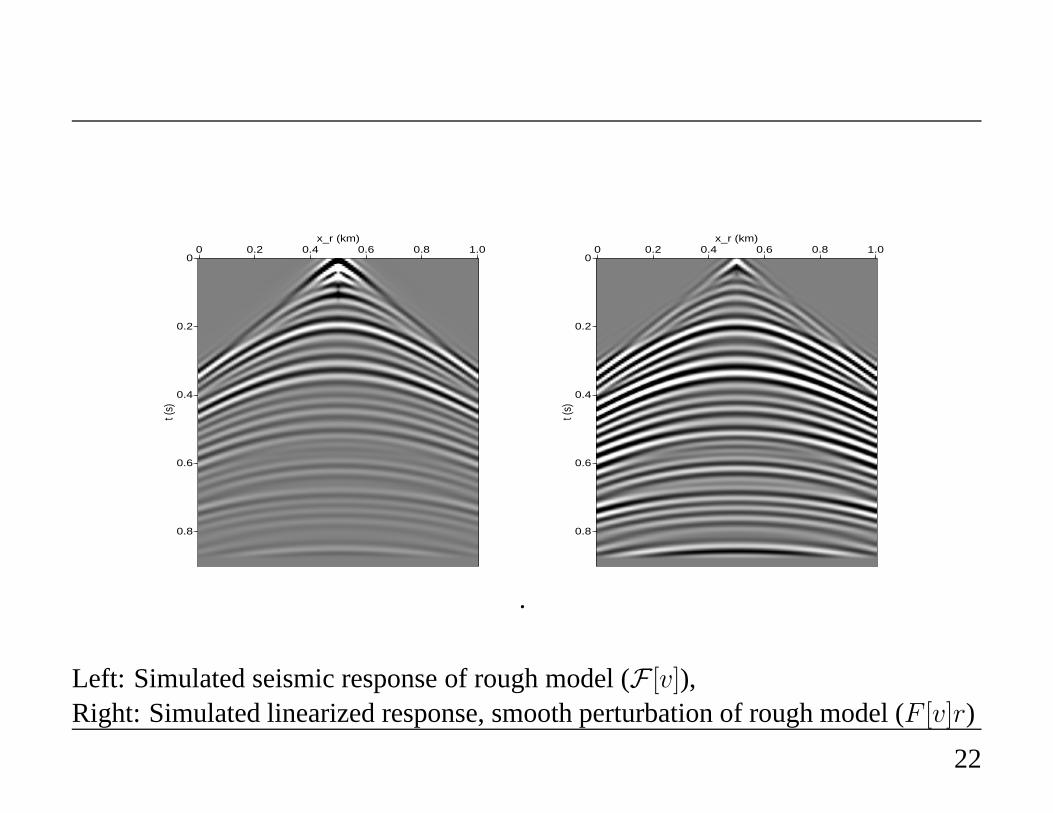
Left: Simulated seismic response of rough model (F [v]),Right: Simulated linearized response, smooth perturbation of rough model (F [v]r)
22
0
0.2
0.4
0.6
0.8
t (s)
0 0.2 0.4 0.6 0.8 1.0x_r (km)
,
0
0.2
0.4
0.6
0.8
t (s)
0 0.2 0.4 0.6 0.8 1.0x_r (km)
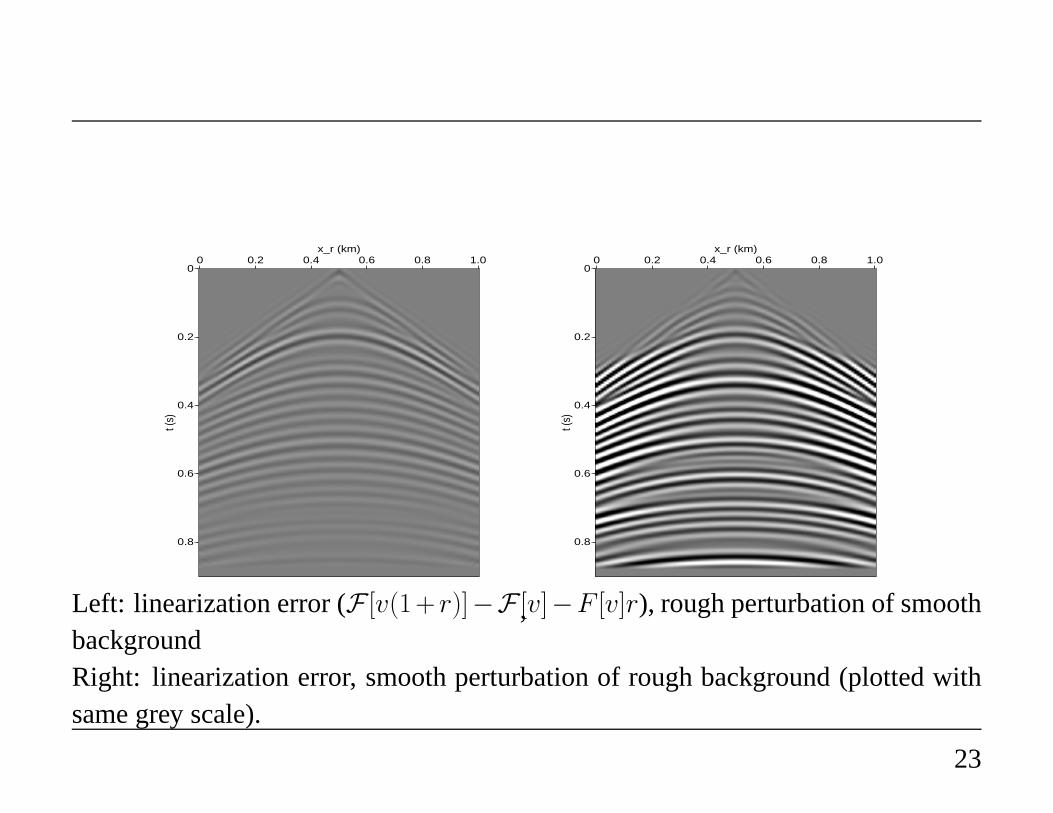
Left: linearization error (F [v(1+ r)]−F [v]−F [v]r), rough perturbation of smoothbackgroundRight: linearization error, smooth perturbation of rough background (plotted withsame grey scale).
23

Summary
• v smooth,r oscillatory⇒ F [v]r approximatesprimary reflection = result ofwave interacting with material heterogeneity only once (single scattering); errorconsists ofmultiple reflections, which are “not too large” ifr is “not too big”,and sometimes can be suppressed.
• v nonsmooth,r smooth⇒ error consists oftime shiftsin waves which are verylarge perturbations as waves are oscillatory.
No mathematical results are known which justify/explain these observations in anyrigorous way, except in 1D.
24
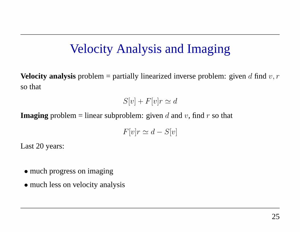
Velocity Analysis and Imaging
Velocity analysisproblem = partially linearized inverse problem: givend find v, r
so that
S[v] + F [v]r ≃ d
Imaging problem = linear subproblem: givend andv, find r so that
F [v]r ≃ d − S[v]
Last 20 years:
• much progress on imaging
• much less on velocity analysis
25

Aymptotic assumption
Linearization is accurate⇔ length scale ofv >> length scale ofr ≃ wavelength,properties ofF [v] dominated by those ofFδ[v] (= F [v] with w = δ). Implicit inmigration concept (eg. Hagedoorn, 1954); explicit use: Cohen & Bleistein, SIAMJAM 1977.
Key idea:reflectors (rapid changes inr) emulatesingularities; reflections(rapidlyoscillating features in data) also emulate singularities.
NB: “everybody’s favorite reflector”: the smooth interfaceacross whichr jumps.But this is an oversimplification - reflectors in the Earth may be complex zones ofrapid change, pehaps in all directions. More flexible notionneeded!!
26
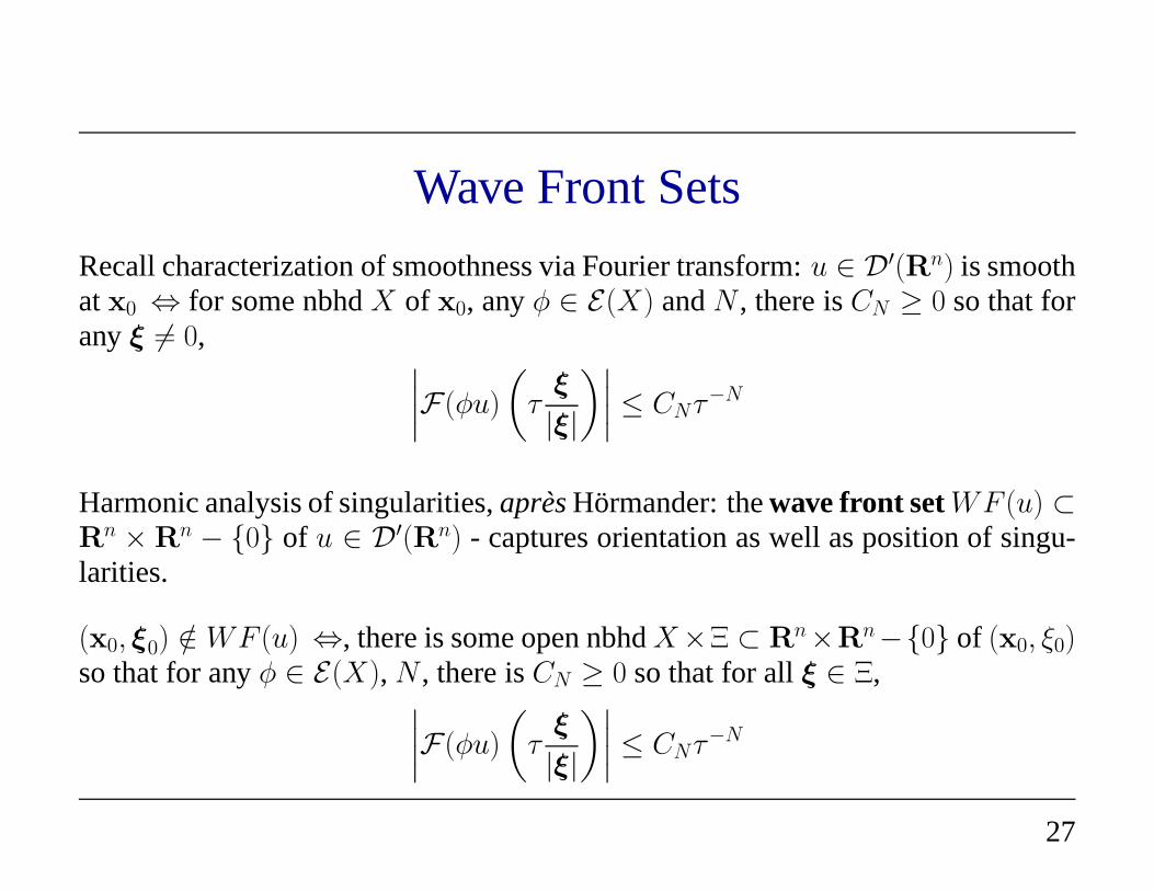
Wave Front Sets
Recall characterization of smoothness via Fourier transform: u ∈ D′(Rn) is smoothatx0 ⇔ for some nbhdX of x0, anyφ ∈ E(X) andN , there isCN ≥ 0 so that foranyξ 6= 0,
∣
∣
∣
∣
F(φu)
(
τξ
|ξ|
)∣
∣
∣
∣
≤ CNτ−N
Harmonic analysis of singularities,apresHormander: thewave front setWF (u) ⊂R
n × Rn − 0 of u ∈ D′(Rn) - captures orientation as well as position of singu-
larities.
(x0, ξ0) /∈ WF (u) ⇔, there is some open nbhdX×Ξ ⊂ Rn×R
n−0 of (x0, ξ0)so that for anyφ ∈ E(X), N , there isCN ≥ 0 so that for allξ ∈ Ξ,
∣
∣
∣
∣
F(φu)
(
τξ
|ξ|
)∣
∣
∣
∣
≤ CNτ−N
27

Housekeeping chores
(i) note that the nbhdsΞ may naturally be taken to becones;
(ii) u is smooth atx0 ⇔ (x0, ξ0) /∈ WF (u) for all ξ0 ∈ Rn − 0;
(iii) WF (u) is invariant under chg. of coords if it is regarded as a subsetof thecotangent bundleT ∗(Rn) (i.e. theξ components transform as covectors).
[Good refs: Duistermaat, 1996; Taylor, 1981; Hormander, 1983]
The standard example: ifu jumps across the interfacef(x) = 0, otherwise smooth,thenWF (u) ⊂ Nf = (x, ξ) : f(x) = 0, ξ||∇f(x) (normal bundleof f = 0).
28

Wavefront set of a jump discontinuity
H(
)=0
φ
φ
=0φ
φ)=1
>0
<0
φH(
ξx
WF (H(φ)) = (x, ξ) : φ(x) = 0, ξ||∇φ(x)
29

Microlocal property of differential operators
Supposeu ∈ D′(Rn), (x0, ξ0) /∈ WF (u), andP (x, D) is a partial differentialoperator:
P (x, D) =∑
|α|≤m
aα(x)Dα
D = (D1, ..., Dn), Di = −i∂
∂xi
α = (α1, ..., αn), |α| =∑
i
αi,
Dα = Dα11 ...Dαn
n
Then(x0, ξ0) /∈ WF (P (x, D)u) [i.e.: WF (Pu) ⊂ WF (u)].
30

Proof
ChooseX × Ξ as in the definition,φ ∈ D(X) form the required Fourier transform∫
dx eix·(τξ)φ(x)P (x, D)u(x)
and start integrating by parts: eventually
=∑
|α|≤m
τ |α|ξα
∫
dx eix·(τξ)φα(x)u(x)
whereφα ∈ D(X) is a linear combination of derivatives ofφ and theaαs. Sinceeach integral is rapidly decreasing asτ → ∞ for ξ ∈ Ξ, it remains rapidly decreas-ing after multiplication byτ |α|, and so does the sum.Q. E. D.
31
Formalizing the reflector concept
Key idea, restated: reflectors (or “reflecting elements”) will be points inWF (r).Reflections will be points inWF (d).
These ideas lead to a usable definition ofimage: a reflectivity modelr is an imageof r if WF (r) ⊂ WF (r) (the closer to equality, the better the image).
Idealizedmigration problem : givend (henceWF (d)) deduce somehow a functionwhich hasthe right reflectors, i.e. a functionr with WF (r) ≃ WF (r).
NB: you’re going to needv! (“It all depends on v(x,y,z)” - J. Claerbout)
32
Integral representation of linearized operator
With w = δ, acoustic potentialu is same as Causal Green’s functionG(x, t;xs) =retarded fundamental solution:
(
1
v2
∂2
∂t2−∇2
)
G(x, t;xs) = δ(t)δ(x − bxs)
andG ≡ 0, t < 0. Then (w = δ!) p = ∂G∂t , δp = ∂δG
∂t , and(
1
v2
∂2
∂t2−∇2
)
δG(x, t;xs) =2
v2(x)
∂2G
∂t2(x, t;xs)r(x)
Simplification: from now on, defineF [v]r = δG|x=xr
- i.e. lose at-derivative.Duhamel’s principle⇒
δG(xr, t;xs) =
∫
dx2r(x)
v(x)2
∫
dsG(xr, t − s;x)∂2G
∂t2(x, s;xs)
33

Add geometric optics...
Geometric optics approximation ofG should be good, asv is smooth. Summary: ifx “not too far” fromxs, then
G(x, t;xs) = a(x;xs)δ(t − τ (x; xs)) + R(x, t;xs)
where the traveltimeτ (x; xs) solves the eikonal equation
v|∇τ | = 1, τ (x;xs) ∼|x − xs|
v(xs), x → xs
and the amplitudea(x;xs) solves the transport equation
∇ · (a2∇τ ) = 0, ...
Refs: Courant & Hilbert, FriedlanderSound Pulses, WWSFoundationsand manyrefs cited there...
34

Simple Geometric Optics
“Not too far” means: there should be one and only one ray of geometric opticsconnecting eachxs or xr to eachx ∈ suppr.
Will call this thesimple geometric opticsassumption.
Within region satisfying simple geometric optics assumption,τ is smooth (x 6= xs)solution of eikonal equation. Effective methods for numerical solution of eikonal,transport equations: ray tracing (Lagrangian), various sorts of upwind finite differ-ence (Eulerian) methods. See eg. Sethian book, WWS 1999 MGSSnotes (online)for details.
35
Caution - caustics!
For “random but smooth”v(x) with varianceσ, more than one connecting ray oc-curs as soon as the distance isO(σ−2/3). Suchmultipathingis invariably accompa-nied by the formation of acaustic= envelope of rays (White, 1982).
Upon caustic formation, the simple geometric optics field description above is nolonger correct.
Failure of GO at caustic understood in 19th century. Generalization of GO to re-gions containing caustics accomplished by Ludwig and Kravtsov, 1966-7, elabo-rated by Maslov, Hormander, Duistermaat, many others.
36

A caustic example (1)
0 0.1 0.2 0.3 0.4 0.5 0.6 0.7 0.8 0.9 1
0
0.2
0.4
0.6
0.8
1
1.2
1.4
1.6
1.8
2
sin1: velocity field
2D Example of strong refraction: Sinusoidal velocity fieldv(x, z) = 1+0.2 sin πz2
sin 3πx
37

A caustic example (2)
0 0.1 0.2 0.3 0.4 0.5 0.6 0.7 0.8 0.9 1
0
0.2
0.4
0.6
0.8
1
1.2
1.4
1.6
1.8
2
sin1: rays with takeoff angles in range 1.41372 to 1.72788
Rays in sinusoidal velocity field, source point = origin. Note formation of caustic,multiple rays to source point in lower center.
38

An oft-forgotten detail
All of this is meaningful only if the remainderR is small in a suitable sense: energyestimate (Exercise!) ⇒
∫
dx
∫ T
0
dt |R(x, t;xs)|2 ≤ C‖v‖C4
(this is an easy, suboptimal estimate - with more work can replace 4 with 2)
If v ∈ C∞, can complete the geometric optics approximation of the Green’s func-tion so that the difference isC∞ - then the two sides have the same singularities, ie.the same wavefront set.
39
Finally, a wave!
The geometric optics approximation to the Green’s function
G(x, t;xs) ≃ a(x;xs)δ(t − τ (x; xs))
describes a (singular) quasi-spherical waves [spherical,if v = const., for thenτ (x,xs) = |x − xs|/v].
Geometric optics is the the best currently available explanation for waves in het-erogeneous media.Note the inadequacy:v must besmooth, but the compressionalvelocity distribution in the Earth varies on all scales!
40

The linearized operator as Generalized Radon
Transform
Assume:supp r contained in simple geometric optics domain (each point reachedby unique ray from any source or receiver point).
Then distribution kernelK of F [v] is
K(xr, t,xs;x) =
∫
dsG(xr, t − s;x)∂2G
∂t2(x, s;xs)
2
v2(x)
≃
∫
ds2a(xr,x)a(x,xs)
v2(x)δ′(t − s − τ (xr,x))δ′′(s − τ (x,xs))
41
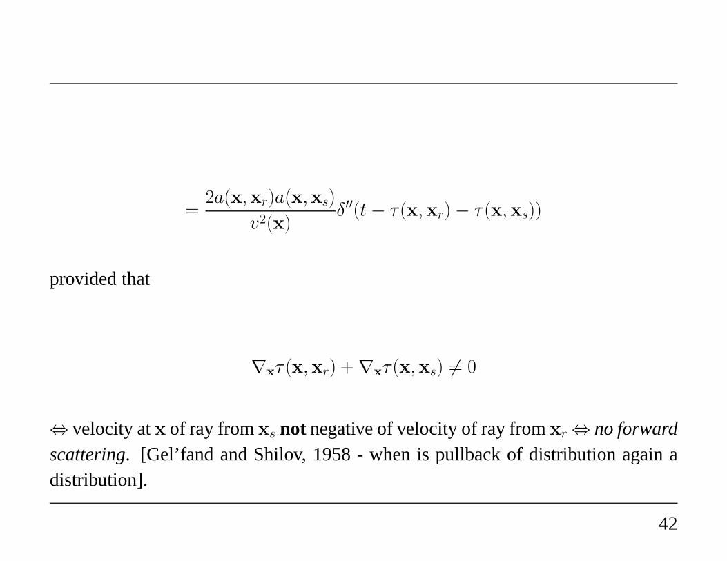
=2a(x,xr)a(x,xs)
v2(x)δ′′(t − τ (x,xr) − τ (x,xs))
provided that
∇xτ (x,xr) + ∇xτ (x,xs) 6= 0
⇔ velocity atx of ray fromxs not negative of velocity of ray fromxr ⇔ no forwardscattering. [Gel’fand and Shilov, 1958 - when is pullback of distribution again adistribution].
42

GRT = “Kirchhoff” modeling
So: forr supported in simple geometric optics domain, no forward scattering⇒
δG(xr, t;xs) ≃
∂2
∂t2
∫
dx2r(x)
v2(x)a(x,xr)a(x,xs)δ(t − τ (x,xr) − τ (x,xs))
That is: pressure perturbation is sum (integral) ofr over reflection isochronx :
t = τ (x,xr) + τ (x,xs), w. weighting, filtering. Note: ifv =const. then isochronis ellipsoid, asτ (xs,x) = |xs − x|/v!
(y,x )+ (y,x )ττt=
x x
y
s
r s
r
43

Zero Offset data and the Exploding Reflector
Zero offset data (xs = xr) is seldom actually measured (contrast radar, sonar!), butroutinelyapproximatedthroughNMO-stack(to be explained later).
Extracting image from zero offset data, rather than from all(100’s) of offsets, istremendousdata reduction- when approximation is accurate, leads to excellentimages.
Imaging basis: theexploding reflectormodel (Claerbout, 1970’s).
44

For zero-offset data, distribution kernel ofF [v] is
K(xs, t,xs;x) =∂2
∂t2
∫
ds2
v2(x)G(xs, t − s;x)G(x, s;xs)
Under some circumstances (explained below),K ( = G time-convolved with itself)is “similar” (also explained) toG = Green’s function forv/2. Then
δG(xs, t;xs) ∼∂2
∂t2
∫
dx G(xs, t,x)2r(x)
v2(x)
∼ solutionw of(
4
v2
∂2
∂t2−∇2
)
w = δ(t)2r
v2
Thus reflector “explodes” at time zero, resulting field propagates in “material” withvelocity v/2.
45

Explain when the exploding reflector model “works”, i.e. when G time-convolvedwith itself is “similar” to G = Green’s function forv/2. If supp r lies in simplegeometry domain, then
K(xs, t,xs;x) =
∫
ds2a2(x,xs)
v2(x)δ(t − s − τ (xs,x))δ′′(s − τ (x,xs))
=2a2(x,xs)
v2(x)δ′′(t − 2τ (x,xs))
whereas the Green’s functionG for v/2 is
G(x, t;xs) = a(x,xs)δ(t − 2τ (x,xs))
(half velocity = double traveltime, same rays!).
46
Difference between effects ofK, G: for eachxs scaler by smooth fcn - preservesWF (r) henceWF (F [v]r) and relation between them. Also: adjoints have sameeffect onWF sets.
Upshot: from imaging point of view (i.e. apart from amplitude, derivative (filter)),kernel ofF [v] restricted to zero offset is same as Green’s function forv/2, providedthat simple geometry hypothesis holds:only one ray connects each source point toeach scattering point, ie.no multipathing.
See Claerbout, IEI, for examples which demonstrate that multipathing really doesinvalidate exploding reflector model.
47
Standard Processing
Inspirational interlude: the sort-of-layered theory =“Standard Processing”
Suppose werev,r functions ofz = x3 only, all sources and receivers atz = 0.Then the entire system is translation-invariant inx1, x2 ⇒ Green’s functionG itsperturbationδG, and the idealized dataδG|z=0 are really only functions oft, z, andhalf-offseth = |xs−xr|/2. There would beonly one seismic experiment, equivalentto anycommon midpoint gather(“CMP”).
This isn’t really true -look at the data!!! However it isapproximatelycorrect inmany places in the world: CMPs change very slowly with midpoint xm = (xr +
xs)/2.
48

Standard processing: treat each CMPas if it were the result of an experiment per-formed over a layered medium, but permit the layers to vary with midpoint.
Thusv = v(z), r = r(z) for purposes of analysis, but at the endv = v(xm, z), r =
r(xm, z).
F [v]r(xr, t;xs)
≃
∫
dx2r(z)
v2(z)a(x, xr)a(x, xs)δ
′′(t − τ (x, xr) − τ (x, xs))
=
∫
dz2r(z)
v2(z)
∫
dω
∫
dxω2a(x, xr)a(x, xs)eiω(t−τ(x,xr)−τ(x,xs))
49

Since we have already thrown away smoother (lower frequency) terms, do it againusingstationary phase.Upshot (see 2000 MGSS notes for details): up to smoother(lower frequency) error,
F [v]r(h, t) ≃ A(z(h, t), h)R(z(h, t))
Herez(h, t) is the inverse of the 2-way traveltime
t(h, z) = 2τ ((h, 0, z), (0, 0, 0))
i.e. z(t(h, z′), h) = z′. R is (yet another version of) “reflectivity”
R(z) =1
2
dr
dz(z)
That is,F [v] is a a derivative followed by a change of variable followed bymulti-plication by a smooth function. Substitutet0 (vertical travel time) forz (depth) andyou get “Inverse NMO” (t0 → (t, h)). Will be sloppy and callz → (t, h) INMO.
50

Anatomy of an adjoint
∫
dt
∫
dh d(t, h)F [v]r(t, h) =
∫
dt
∫
dh d(t, h)A(z(t, h), h)R(z(t, h))
=
∫
dz R(z)
∫
dh∂t
∂z(z, h)A(z, h)d(t(z, h), h) =
∫
dz r(z)(F [v]∗d)(z)
soF [v]∗ = − ∂∂z
SM [v]N [v], where
• N [v] = NMO operator N [v]d(z, h) = d(t(z, h), h)
• M [v] = multiplication by ∂t∂z
A
• S = stacking operatorSf(z) =∫
dh f(z, h)
51

Normal Op is PDO⇒ Imaging
F [v]∗F [v]r(z) = −∂
∂z
[∫
dhdt
dz(z, h)A2(z, h)
]
∂
∂zr(z)
Microlocal property of PDOs⇒ WF (F [v]∗F [v]r) ⊂ WF (r) i.e. F [v]∗ is an imag-ing operator.
If you leave out the amplitude factor (M [v]) and the derivatives, as is commonlydone, then you get essentially the same expression - so (NMO,stack) is an imagingoperator!
It’s even easy to get an (asymptotic) inverse out of this - exercise for the reader.
Now make everything dependent onxm and you’ve got standard processing. (endof layered interlude).
52

But the Earth is not layered!
In general,
Is F [v]∗ an imaging operator?
What sort of thing isF [v]∗F [v]??
Stay tuned!
53

Mathematics of Seismic ImagingPart II
William W. Symes
PIMS, June 2005
Review: Normal Operators and imaging
If d = F [v]r, then
F [v]∗d = F [v]∗F [v]r
Recall: In the layered case,F [v]∗F [v] is an operator which preserves wave frontsets.
WheneverF [v]∗F [v] preserves wave front sets,F [v]∗ is an imaging operator.
1

Review: Generalized Radon Representation
Assume (1)r (oscillatory) supported in simple geometric optics domainfor v (smooth),(2) no forward scattering. Then
F [v]r(xr, t;xs) ≃
∫
dx2r(x)
v2(x)a(x,xr)a(x,xs)δ
′′(t− τ (x,xr) − τ (x,xs))
Similar representation of adjoint follows:
F [v]∗d(x) =
∫ ∫ ∫
dxr dxs dt a(x,xr)a(x,xs)δ′′(t−τ (x;xs)−τ (x;xr))d(xr, t;xs)
2

Beylkin, J. Math. Phys.1985
For r supported in simple geometric optics domain,
•WF (F [v]∗F [v]r) ⊂WF (r)
• if d = F [v]+F [v]r (data consistent with linearized model), thenF [v]∗(d−F [v])
is an image ofr
• an operatorF [v]† exists for whichF [v]†(d−F [v])− r is smootherthanr, undersome constraints onr - an inverse modulo smoothing operatorsor parametrix.
3

Outline of proof
ExpressF [v]∗F [v] as “Kirchhoff modeling” followed by “Kirchhoff migration”;(ii) introduce Fourier transform; (iii) approximate for large wavenumbers usingstationary phase, leads to representation ofF [v]∗F [v] modulo smoothing error aspseudodifferential operator(“ΨDO”):
F [v]∗F [v]r(x) ≃ p(x, D)r(x) ≡
∫
dξ p(x, ξ)eix·ξr(ξ)
in which p ∈ C∞, and for somem (theorder of p), all multiindicesα, β, and allcompactK ⊂ R
n, there exist constantsCα,β,K ≥ 0 for which
|DαxD
β
ξp(x, ξ)| ≤ Cα,β,K(1 + |ξ|)m−|β|, x ∈ K
Explicit computation ofsymbol p - for details, see Notes on Math Foundations.
4

Microlocal PropertyofΨDOs
:
if p(x,D) is aΨDO, u ∈ E ′(Rn) thenWF (p(x,D)u) ⊂ WF (u).
Will prove this, from which imaging property of prestack Kirchhoff migration fol-lows. First, a few other properties:
• differential operators areΨDOs (easy - exercise)
• ΨDOs of orderm form a module overC∞(Rn) (also easy)
• product ofΨDO orderm, ΨDO orderl = ΨDO order≤ m + l; adjoint ofΨDOorderm is ΨDO orderm (harder)
Complete accounts of theory, many apps: books of Duistermaat, Taylor, Nirenberg,Treves, Hormander.
5

Proof of Microlocal Property
Suppose(x0, ξ0) /∈ WF (u), choose neighborhoodsX, Ξ as in defn, withΞ conic.Need to choose analogous nbhds forP (x,D)u. Pick δ > 0 so thatB3δ(x0) ⊂ X,setX ′ = Bδ(x0).
Similarly pick 0 < ǫ < 1/3 so thatB3ǫ(ξ0/|ξ0|) ⊂ Ξ, and choseΞ′ = τξ : ξ ∈
Bǫ(ξ0/|ξ0|), τ > 0.
Need to chooseφ ∈ E ′(X ′), estimateF(φP (x, D)u). Chooseψ ∈ E(X) so thatψ ≡ 1 onB2δ(x0).
NB: this implies that ifx ∈ X ′, ψ(y) 6= 1 then|x − y| ≥ δ.
6

Write u = (1 − ψ)u + ψu. Claim: φP (x, D)((1 − ψ)u) is smooth.
φ(x)P (x, D)((1 − ψ)u))(x)
= φ(x)
∫
dξ P (x, ξ)eix·ξ∫
dy (1 − ψ(y))u(y)e−iy·ξ
=
∫
dξ
∫
dy P (x, ξ)φ(x)(1 − ψ(y))ei(x−y)·ξu(y)
=
∫
dξ
∫
dy (−∇2ξ)MP (x, ξ)φ(x)(1 − ψ(y))|x − y|−2Mei(x−y)·ξu(y)
7
using the identity
ei(x−y)·ξ = |x − y|−2[
−∇2ξei(x−y)·ξ
]
and integrating by parts2M times in ξ. This is permissible becauseφ(x)(1 −
ψ(y)) 6= 0 ⇒ |x − y| > δ.
According to the definition ofΨDO,
|(−∇2ξ)MP (x, ξ)| ≤ C|ξ|m−2M
For anyK, the integral thus becomes absolutely convergent afterK differentiationsof the integrand, providedM is chosen large enough. Q.E.D. Claim.
This leaves us withφP (x, D)(ψu). Pickη ∈ Ξ′ and w.l.o.g. scale|η| = 1.
8

Fourier transform:
F(φP (x, D)(ψu))(τη) =
∫
dx
∫
dξ P (x, ξ)φ(x)ψu(ξ)eix·(ξ−τη)
Introduceτθ = ξ, and rewrite this as
= τn∫
dx
∫
dθ P (x, τθ)φ(x)ψu(τθ)eiτx·(θ−η)
Divide the domain of the inner integral intoθ : |θ − η| > ǫ and its complement.Use
−∇2xeiτx·(θ−η) = τ 2|θ − η|2eiτx·(θ−η)
9
Integrate by parts2M times to estimate the first integral:
τn−2M
∣
∣
∣
∣
∫
dx
∫
|θ−η|>ǫ
dθ (−∇2x)M [P (x, τθ)φ(x)]ψu(τθ)
× |θ − η|−2Meiτx·(θ−η)∣
∣
∣
≤ Cτn+m−2M
m being the order ofP . Thus the first integral is rapidly decreasing inτ .
10

For the second integral, note that|θ − η| ≤ ǫ ⇒ θ ∈ Ξ, per the defn ofΞ′. SinceX × Ξ is disjoint from the wavefront set ofu, for a sequence of constantsCN ,|ψu(τθ)| ≤ CNτ
−N uniformly for θ in the (compact) domain of integration, whencethe second integral is also rapidly decreasing inτ . Q. E. D.
And that’s why Kirchhoff migration works, at least in the simple geometric opticsregime.
11

Inversion aperture
Γ[v] ⊂ R3 × R
3 − 0:
if WF (r) ⊂ Γ[v], thenWF (F [v]∗F [v]r) = WF (r) andF [v]∗F [v] “acts invertible”.[construction ofΓ[v] - later!]
Beylkin: with proper choice of amplitudeb(xr, t;xs), the modified Kirchhoff mi-gration operator
F [v]†d(x) =
∫ ∫ ∫
dxr dxs dt b(xr, t;xs)δ(t− τ (x; xs) − τ (x;xr))d(xr, t;xs)
yieldsF [v]†F [v]r ≃ r if WF (r) ⊂ Γ[v]
12

For details of Beylkin construction: Beylkin, 1985; Milleret al 1989; Bleistein,Cohen, and Stockwell 2000; WWS Math Foundations, MGSS notes1998. Allcomponents are by-products of eikonal solution.
aka: Generalized Radon Transform (“GRT”) inversion, Ray-Born inversion, migra-tion/inversion, true amplitude migration,...
Many extensions, eg. to elasticity: Bleistein, Burridge, deHoop, Lambare,...
Apparent limitation: construction relies on simple geometric optics (no multipathing)- is this really necessary?
13

0
500
1000
1500
2000
2500
Dep
th in
Met
ers
0 200 400 600 800 1000 1200 1400CDP
Example of GRT Inversion (application ofF [v]†): K. Araya (1995), “2.5D” in-version of marine streamer data from Gulf of Mexico: 500 source positions, 120receiver channels, 750 Mb.
14

Why Beylkin isn’t enough
The theory developed by Beylkin and others cannot be the end of the story:
• The “single ray” hypotheses generally fails in the presenceof strong refraction.
• B. White, “The Stochastic Caustic” (1982): For “random but smooth”v(x) withvarianceσ, points at distanceO(σ−2/3) from source have more than one rayconnecting to source, with probability 1 -multipathingassociated with formationof caustics= ray envelopes.
• Formation of caustics invalidates asymptotic analysis on which Beylkin result isbased.
15
Why it matters
• Strong refraction leading to multipathing and caustic formation typical of salt(4-5 km/s) intrusion into sedimentary rock (2-3 km/s) (eg. Gulf of Mexico),also chalk tectonics in North Sea and elsewhere - some of the most promisingpetroleum provinces!
16

Escape from simplicity - the Canonical Relation
How do we get away from “simple geometric optics”, SSR, DSR,... - all violatedin sufficiently complex (and realistic) models? RakeshComm. PDE1988, NolanComm. PDE1997: global description ofFδ[v] as mapping reflectors7→ reflections.
Y = xs, t,xr (time × set of source-receiver pairs) submfd ofR7 of dim. ≤ 5,
Π : T ∗(R7) → T ∗Y the natural projection
supp r ⊂ X ⊂ R3
Canonical relationCFδ[v] ⊂ T ∗(X) − 0 × T ∗(Y ) − 0 describes singularitymapping properties ofF :
(x, ξ,y, η) ∈ CFδ[v] ⇔
for someu ∈ E ′(X), (x, ξ) ∈WF (u), and (y, η) ∈WF (Fu)
17

Rays Construction of the Relation
Rays of geometric optics: solutions of Hamiltonian system
dX
dt= ∇ΞH(X,Ξ),
dΞ
dt= −∇XH(X,Ξ)
with H(X,Ξ) = 12[1 − v2(X)|Ξ|2] = 0 (null bicharacteristics).
Characterization of CF :
((x, ξ), (xs, t,xr, ξs, τ, ξr)) ∈ CFδ[v] ⊂ T ∗(X) − 0 × T ∗(Y ) − 0
⇔ there arerays of geometric optics(Xs,Ξs), (Xr,Ξr) and timests, tr so that
Π(Xs(0), t,Xr(t),Ξs(0), τ,Ξr(t)) = (xs, t,xr, ξs, τ, ξr),
Xs(ts) = Xr(t− tr) = x, ts + tr = t, Ξs(ts) − Ξr(t− tr)||ξ
18

SinceΞs(ts), −Ξr(t − tr) have same length, sum = bisector⇒ velocity vectors ofincident ray from source and reflected ray from receiver (traced backwards in time)make equal angles with reflector atx with normalξ.
Upshot: canonical relation ofFδ[v] simply enforces the equal-angles law of reflec-tion.
Further,rays carry high-frequency energy, in exactly the fashion that seismologistsimagine.
Finally,Rakesh’s characterization ofCF is global: no assumptions about ray geom-etry, other than no forward scattering and no grazing incidence on the acquisitionsurfaceY , are needed.
19

The Picture
−Ξ
X
s
r
Ξ (t )s
r (t )
X s
x
x x ξ rs, r,sξ,
Ξ s
ξ,
rΞr,
,
ΠΠ
20

Proof: Plan of attack
Recall that
F [v]r(xr, t;xs) =∂δu
∂t(xr, t;xs)
where
1
v2
∂2δu
∂t2−∇2δu =
1
v2
∂2u
∂t2r
1
v2
∂2u
∂t2−∇2u = δ(t)δ(x − xs)
andu, δu ≡ 0, t < 0.
Need to understand (1)WF (u), (2) relationWF (r) ↔ WF (ru), (3)WF of solnof WE in terms ofWF of RHS (this also gives (1)!).
21

Singularities of the Acoustic Potential Field
Main tool: Propagation of Singularities theorem of Hormander (1970).
Given symbolp(x, ξ), order m, with asymptotic expansion, definenull bicharater-istics(= rays) as solutions(x(t), ξ(t)) of Hamiltonian system
dx
dt=∂p
∂ξ(x, ξ),
dξ
dt= −
∂p
∂x(x, ξ)
with p(x(t), ξ(t)) ≡ 0.
Theorem: Supposep(x, D)u = f , and suppose that fort0 ≤ t ≤ t1, (x(t), ξ(t)) /∈
WF (f). Then either(x(t), ξ(t)) : t0 ≤ t ≤ t1 ⊂ WF (u) or (x(t), ξ(t)) : t0 ≤
t ≤ t1 ⊂ T ∗(Rn) −WF (u).
22
Source to Field
RHS of wave equation foru = δ function inx, t. WF set =(x, t, ξ, τ ) : x = xs, t =
0 - i.e. no restriction on covector part.
⇒ (x, t, ξ, τ ) ∈ WF (u) iff a ray starting at(xs, 0) passes over(x, t) - i.e. (x, t)
lies on the “light cone” with vertex at(xx, 0). Symbol for wave op isp(x, t, ξ, τ ) =12(τ 2 − v2(x)|ξ|2), so Hamilton’s equations for null bicharacteristics are
dX
dt= −v2(X)Ξ,
dΞ
dt= ∇ log v(X)
Thusξ is proportional to velocity vector of ray.
[(ξ, τ ) normal to light cone.]
23
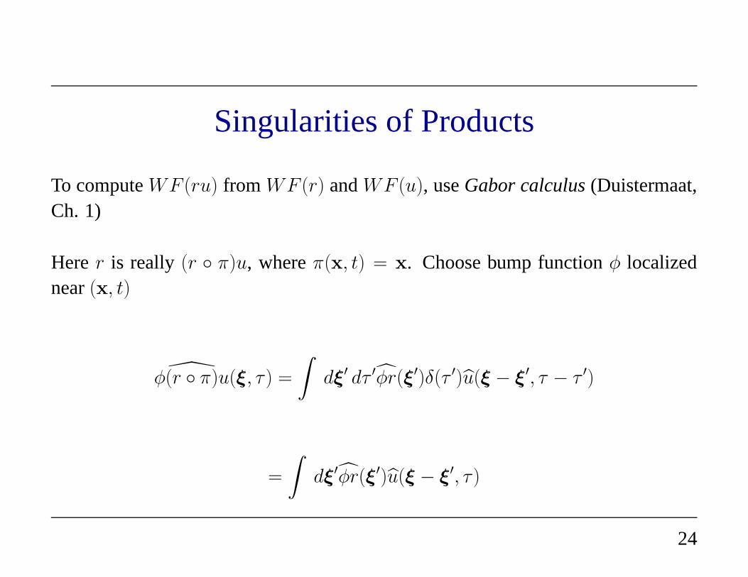
Singularities of Products
To computeWF (ru) fromWF (r) andWF (u), useGabor calculus(Duistermaat,Ch. 1)
Herer is really (r π)u, whereπ(x, t) = x. Choose bump functionφ localizednear(x, t)
φ(r π)u(ξ, τ ) =
∫
dξ′ dτ ′φr(ξ′)δ(τ ′)u(ξ − ξ′, τ − τ ′)
=
∫
dξ′φr(ξ′)u(ξ − ξ′, τ )
24

This will decay rapidly as|(ξ, τ )| → ∞ unless (i) you can find(x′, ξ′) ∈ WF (r)
so thatx,x′ ∈ π(suppφ), ξ − ξ′ ∈ WF (u), i.e. (ξ, τ ) ∈ WF (r π) + WF (u), or(ii) ξ ∈ WF (r) or (ξ, τ ) ∈ WF (u).
Possibility (ii) will not contribute, so effectively
WF ((r π)u) = (x, ts, ξ + Ξs(ts), ·) : (x, ξ) ∈WF (r), x = Xs(ts)
for a ray(Xs,Ξs) with Xs(0) = xs, someτ .
25

Wavefront set of Scattered Field
Once again use propagation of singularities:(xr, t, ξr, τr) ∈ WF (δu) ⇔ on ray(Xr,Ξr) passing throughWF (ru). Can argue that time of intersection ist− tr < t.
That is,
Xr(t) = xr,Xr(t− tr) = Xs(ts) = x,
t = tr + ts, and
Ξr(ts) = ξ + Ξs(ts)
for someξ ∈ WF (r). Q. E. D.
26

Rakesh’s Thesis
Rakesh also showed thatF [v] is aFourier Integral Operator= class of oscillatoryintegral operators, introduced by Hormander and others in the ’70s to describe thesolutions of nonelliptic PDEs.
Phases and amplitudes of FIOs satisfy certain restrictive conditions. Canonicalrelations have geometric description similar to that ofF [v]. Adjoint of FIO is FIOwith inverse canonical relation.
ΨDOs are special FIOs, as are GRTs.
Composition of FIOs doesnot yield an FIO in general. Beylkin had shown thatF [v]∗F [v] is FIO (ΨDO, actually) under simple ray geometry hypothesis - but thisis only sufficient. Rakesh noted that this follows from general results of Hormander:simple ray geometry⇔ canonical relation is graph of ext. deriv. of phase function.
27

The Shell Guys and TIC
Smit, tenKroode and Verdel (1998): provided that
• source, receiver positions(xs,xr) form anopen4D manifold (“complete cover-age” - all source, receiver positions at least locally), and
• theTraveltime Injectivity Condition(“TIC”) holds: C−1F [v] ⊂ T ∗Y −0×T ∗X−
0 is afunction- that is, initial data for source and receiver rays and totaltraveltime together determine reflector uniquely.
thenF [v]∗F [v] is ΨDO ⇒ application ofF [v]∗ produces image, andF [v]∗F [v] hasmicrolocal parametrix (“asymptotic inversion”).
28
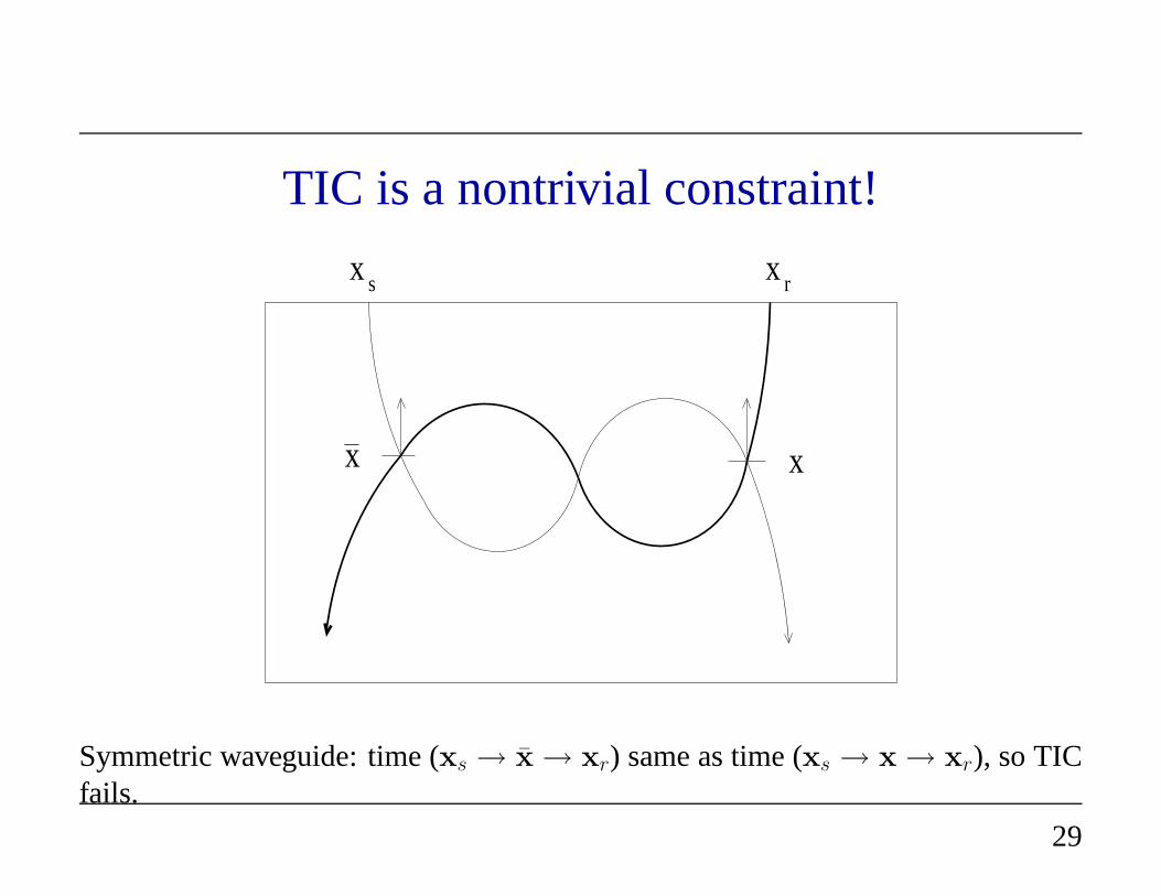
TIC is a nontrivial constraint!
x x
x xs r
Symmetric waveguide: time (xs → x → xr) same as time (xs → x → xr), so TICfails.
29

Stolk’s Thesis
Stolk (2000): under “complete coverage” hypothesis,v for which F [v]∗F [v] is =[ΨDO + rel. smoothing op] form open, dense set (without assuming TIC!).
NB: application ofF [v]∗ involves accounting forall rays connecting source andreceiver with reflectors. Standard practice still attemptsimaging with single choiceof ray pair (shortest time, max energy,...). Operto et al (2000) give nice illustrationthat all rays must be included.
30

Nolan’s Thesis
Limitation of Smit-tenKroode-Verdel: most idealized dataacquisition geometriesviolate “complete coverage”: for example, idealized marine streamer geometry(src-recvr submfd is 3D)
Nolan (1997): result remains true without “complete coverage” condition: requiresonly TIC plus addl condition so that projectionCF [v] → T ∗Y is embedding - butexamples violating TIC are much easier to construct when source-receiver submfdhas positive codim.
Sinister Implication: When data is just a single gather - common shot, commonoffset - image may containartifacts, i.e. spurious reflectors not present in model.
31

Horrible Example I
Synthetic 2D Example (Stolk and WWS, 2001 -Geophysics2004)
Strongly refracting acoustic lens (v) over horizontal reflector (r), d = F [v]r.
(i) for open source-receiver set,F [v]∗d = good image of reflector - within limits offinite frequency implied by numerical method,F [v]∗F [v] acts likeΨDO;
(ii) for common offsetsubmfd (codim 1), TIC is violated andWF (F [v]∗d) is largerthanWF (r).
32

2
1
0
x2
-1 0 1x1
1
0.6
Gaussian lens velocity model, flat reflector at depth 2 km, overlain with rays andwavefronts (Stolk & S. 2002 SEG).
33

5
4
time
HsL
-2 -1 0 1 2receiver position HkmL
Typical shot gather - lots of arrivals
34
1.6
2.0
2.4
x2
0 1 2offset
3,2
3,1
1,2
2,1
3,3
1,1
travel time # s,r
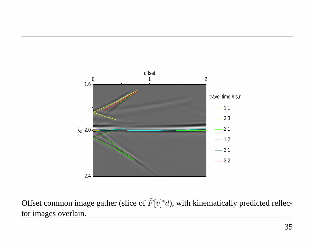
Offset common image gather (slice ofF [v]∗d), with kinematically predicted reflec-tor images overlain.
35

Horrible Example II
Stolk and Symes,Geophysics2004: “Marmouflat” model = smoothed Marmousi(Versteeg & Grau 1991) with two flat reflectors.
2
1
0
z
HkmL
3 4 5 6 7 8 9x HkmL
5.5 kms
1.5 kms
36

2.8
2.6
2.4
2.2
2
1.8
time
HsL
5.2 5.6 6 6.4 6.8 7.2receiver position HkmL
Typical shot gather: much evidence of multipathing, caustic formation.
37

2.2
2.4
2.6
z (k
m)
0 20 40 60 80angle (deg)
Typical common scattering angle image gather: note nonflat event in box - resultsfrom data event migrating alongwrong ray pair.
38

2.4
2
1.6
1.2
0.8
0.4
0
z
HkmL
5.6 6 6.4 6.8 7.2 7.6x HkmL
Blue rays = energy path producing data event. Black rays: energy path for migra-tion, resulting in displaced, angle-dependent image artifact.
39
What it all means
Note that a gather scheme makes the scattering operator block-diagonal: for exam-ple with data sorted into common offset gathersh = (xr − xs)/2,
F [v] = [Fh1[v], ..., FhN [v]]T , d = [dh1, ..., dhN ]T
ThusF [v]∗d =∑
i Fhi[v]∗dhi. Otherwise put: to form image,migrate ith gather
(apply migration operatorFhi[v]∗, then stack individual migrated images (hence
prestack migration).
Horrible Examples show that individual migrated images maycontain nonphysicalapparent reflectors (artifacts).
Smit-tenKroode-Verdel, Nolan, Stolk: if TIC holds, then these artifacts are not sta-tionary with respect to the gather parameter, hencestack out(interfere destructively)in final image.
40


Mathematics of Seismic Imaging
Part II - addendum on Wave Equation
Migration
William W. Symes
PIMS, July 2005

Wave Equation Migration
Techniques for computingF [v]∗:
(i) Reverse time
(ii) Reverse depth
1

Reverse Time Migration, Zero Offset
Start with the zero-offset case - easier, but only if you replace it with the explodingreflector model, which replacesF [v] by
F [v]r(xs, t) = w(xs, t), xs ∈ Xs, 0 ≤ t ≤ T
(
4
v2
∂2
∂t2−∇2
)
w = δ(t)2r
v2, w ≡ 0, t < 0
To compute the adjoint, start with its definition: choosed ∈ E(Xs × (0, T )), so that
< F [v]∗d, r >=< d, F [v]r >
=
∫
Xs
dxs
∫ T
0
dt d(xs, t)w(xs, t)
2

The only thing you know aboutw is that it solves a wave equation withr on theRHS. To get this fact into play, (i) rewrite the integral as a space-time integral:
=
∫
R3dx
∫ T
0
dt
∫
Xs
dxs d(xs, t)δ(x − xs)w(x, t)
(ii) write the other factor in the integrand as the image of a fieldq under the (adjointof the) wave operator (it’s self-adjoint), that is,
(
4
v2
∂2
∂t2−∇2
)
q(x, t) =
∫
Xs
dxs d(xs, t)δ(x − xs)
so
=
∫
R3dx
∫ T
0
dt
[(
4
v2(x)
∂2
∂t2−∇2
)
q(x, t)
]
w(x, t)
3

(iii) integrate by parts
=
∫
R3dx
∫ T
0
dt
[(
4
v2(x)
∂2
∂t2−∇2
)
w(x, t)
]
q(x, t)
which works ifq ≡ 0, t > T (final value condition); (iv) use the wave equation forw
=
∫
R3dx
∫ T
0
dt2
v(x)2r(x)δ(t)q(x, t)
(v) observe that you have computed the adjoint:
=
∫
R3dx r(x)
[
2
v(x)2q(x, 0)
]
=< r, F [v]∗d >
i.e.
F [v]∗d =2
v(x)2q(x, 0)
4

Summary of the computation, with the usual description:
• Use that data as sources, backpropagate in time - i.e. solve the final value (“re-verse time”) problem
(
4
v2
∂2
∂t2−∇2
)
q(x, t) =
∫
Xs
dxs d(xs, t)δ(x − xs), q ≡ 0, t > T
• read out the “image” (= adjoint output) att = 0:
F [v]∗d =2
v(x)2q(x, 0)
Note: The adjoint (time-reversed) fieldq is not the physical field (δu) run back-wards in time, contrary to some imputations in the literature.
5

Historical Remarks
• Known as “two way reverse time finite difference poststack migration” in geo-physical literature (Whitmore, 1982)
• uses full (two way) wave equation, propagates adjoint field backwards in time,generally implemented using finite difference discretization.
• Same as “adjoint state method”, Lions 1968, Chavent 1974 forcontrol and in-verse problems for PDEs - much earlier for control of ODEs - Lailly, Tarantola’80s.
• My buddy Tapia says: all you’re doing is transposing a matrix! True (afterdiscretization), but it’s important that these matrices are triangular, so can beimplemented by recursions - forward for simulation, backwards for adjoint.
6

Reverse Time Migration, Prestack
A slightly messier computation computes the adjoint ofF [v] (i.e. multioffset orprestackmigration):
F [v]∗d(x) = −2
v(x)
∫
dxs
∫ T
0
dt
(
∂q
∂t∇2u
)
(x, t;xs)
whereadjoint fieldq satisfiesq ≡ 0, t ≥ T and
(
1
v2
∂2
∂t2−∇2
)
q(x, t;xs) =
∫
dxr d(xr, t;xs)δ(x − xr)
7

Proof
< F [v]∗d, r >=< d, F [v]r >
=
∫ ∫
dxs dxr
∫ T
0
dt d(xr, t;xs)∂δu
∂t(xr, t;xs)
=
∫
dxs
∫
dx
∫ T
0
dt
∫
dxr d(xr, t;xs)δ(x − xr)
∂δu
∂t(x, t;xs)
=
∫
dxs
∫
dx
∫ T
0
dt
[(
1
v2
∂2
∂t2−∇2
)
q
]
∂δu
∂t(x, t;xs)
8

= −
∫
dxs
∫
dx
∫ T
0
dt
[(
1
v2
∂2
∂t2−∇2
)
δu
]
∂q
∂t(x, t;xs)
(boundary terms in integration by parts vanish because (i)δu ≡ 0, t << 0; (ii)q ≡ 0, t >> 0; (iii) both vanish for largex, at eacht)
= −
∫
dxs
∫
dx
∫ T
0
dt
(
2r
v2
∂2u
∂t2∂q
∂t
)
(x, t;xs)
= −
∫
dxs
∫
dx r(x)2
v2(x)
∫ T
0
dt
(
∂2u
∂t2∂q
∂t
)
(x, t;xs)
=< r, F [v]∗d >
q.e.d.
9

Implementation
Algorithm: finite difference or finite element discretization in x, finite differencetime stepping.
• For eachxs, solve wave equation foru forward in t, record final (t=T) Cauchydata, also (for example) Dirichlet boundary data.
• Stepu andq backwards in time together; at each time step, data serves assourcefor q (“backpropagate data”)
• During backwards time stepping, accumulate (approximations to)
Q(x)+ =2
v2(x)
∫ T
0
dt
(
∂2u
∂t2∂q
∂t
)
(x, t;xs)
(“crosscorrelate reference and backpropagated field”).
• nextxs - after lastxs, F [v]∗d = Q.
10

Reverse Depth Migration, Zero Offset
aka: depth extrapolation, downward continuation, or simply “wave equation migra-tion”.
Introduced by Claerbout, early 70’s (“swimming pool equation”). Again, assumeexploding reflector model:
F [v]r(xs, t) = w(xs, t), xs ∈ Xs, 0 ≤ t ≤ T
(
4
v2
∂2
∂t2−∇2
)
w = δ(t)2r
v2, w ≡ 0, t < 0
Basic idea: 2nd order wave equation permits waves to move in all directions, butwaves carrying reflected energy are (mostly) movingup. Should satisfy a 1st orderequation for wave motion in one direction.
11
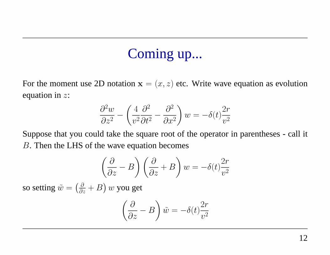
Coming up...
For the moment use 2D notationx = (x, z) etc. Write wave equation as evolutionequation inz:
∂2w
∂z2−
(
4
v2
∂2
∂t2−
∂2
∂x2
)
w = −δ(t)2r
v2
Suppose that you could take the square root of the operator inparentheses - call itB. Then the LHS of the wave equation becomes
(
∂
∂z− B
)(
∂
∂z+ B
)
w = −δ(t)2r
v2
so settingw =(
∂∂z + B
)
w you get(
∂
∂z− B
)
w = −δ(t)2r
v2
12

Some issues
Thismightbe the required equation for upcoming waves.
Two major problems: (i) how the h–l do you take the square rootof a PDO?
(ii) what guarantees that the equation just written governsupcoming waves?
Answers to be found in the theory ofΨDOs!
13

ClassicalΨDOs
Importantsubclassof classicalΨDOs: those whose (“classical”) symbols haveasymptotic expansions:
p(x, ξ) ∼∑
j≤m
pj(x, ξ), |ξ| → ∞
in whichpj is homogeneous inξ of degreej:
pj(x, τξ) = τ jpj(x, τξ), τ, |ξ| ≥ 1
Theprincipal symbolis the homogeneous term of highest degree, i.e.pm above.
14

Products ofΨDOs areΨDOs.
ClassicalΨDOs have more completecalculus, including prescriptions for “com-puting” adjoints, products, and the like. From now on unlessotherwise stated, allΨDOs are classical.
Product rule forΨDOs: if p1, p2 are classical,
p1(x, ξ) =∑
j≤m1
p1j(x, ξ), p2(x, ξ) =
∑
j≤m2
p2j(x, ξ)
then so isp1(x, D)p2(x, D), and its principal symbol isp1m1(x, ξ)p2
m2(x, ξ), andthere is an algorithm for computing the rest of the expansion.
In an open neighborhoodX × Ξ of (x0, ξ0), symbol ofp1(x, D)p2(x, D) dependsonly on symbols ofp1, p2 in X × Ξ.
15
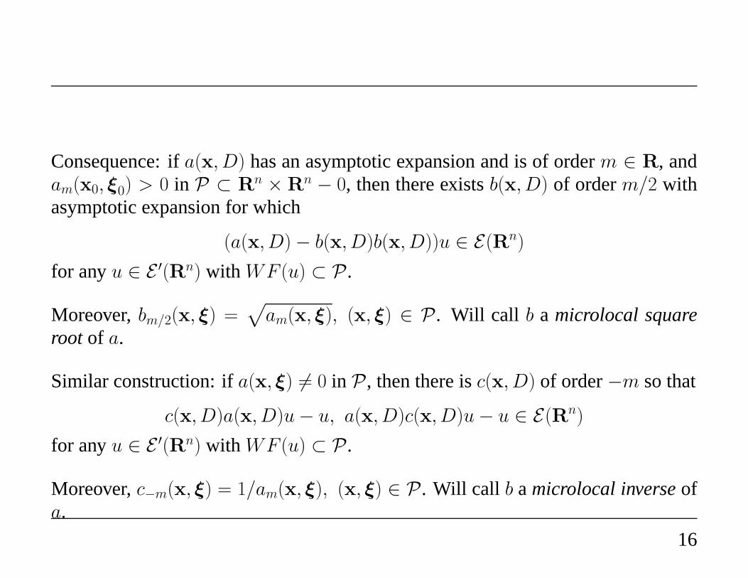
Consequence: ifa(x, D) has an asymptotic expansion and is of orderm ∈ R, andam(x0, ξ0) > 0 in P ⊂ R
n × Rn − 0, then there existsb(x, D) of orderm/2 with
asymptotic expansion for which
(a(x, D) − b(x, D)b(x, D))u ∈ E(Rn)
for anyu ∈ E ′(Rn) with WF (u) ⊂ P.
Moreover,bm/2(x, ξ) =√
am(x, ξ), (x, ξ) ∈ P. Will call b a microlocal squareroot of a.
Similar construction: ifa(x, ξ) 6= 0 in P, then there isc(x, D) of order−m so that
c(x, D)a(x, D)u − u, a(x, D)c(x, D)u − u ∈ E(Rn)
for anyu ∈ E ′(Rn) with WF (u) ⊂ P.
Moreover,c−m(x, ξ) = 1/am(x, ξ), (x, ξ) ∈ P. Will call b a microlocal inverseofa.
16

Application: the Square Root Operator
a(x, z,Dt, Dx) =∂2
∂x2−
4
v(x, z)2∂2
∂t2=
4
v(x, z)2D2
t − D2x
is
a(x, z, τ, ξ) =4
v(x, z)2τ 2 − ξ2
For δ > 0, set
Pδ(z) =
(x, t, ξ, τ ) :4
v(x, z)2τ 2 > (1 + δ)ξ2
17

The SSR Operator
Then according to the last slide, there is an order 1ΨDO-valued function ofz,b(x, z, Dt, Dx), with principal symbol
b1(x, z, τ, ξ) =
√
4
v(x, z)2τ 2 − ξ2 = τ
√
4
v(x, z)2−
ξ2
τ 2, (x, t, ξ, τ ) ∈ Pδ(z)
for whicha(x, z,Dt, Dx)u ≃ b(x, z, Dt, Dx)b(x, z, Dt, Dx)u if WF (u) ⊂ Pδ(z).
b is the world-famoussingle square root (“SSR”) operator - see Claerbout, IEI.
18

The SSR Assumption
To what extent has this construction factored the wave operator:
(
∂
∂z− ib(x, z,Dx, Dt)
)(
∂
∂z+ ib(x, z, Dx, Dt)
)
=∂2
∂z2+ b(x, z, Dx, Dt)b(x, z,Dx, Dt) +
∂b
∂z(x, z,Dx, Dt)
SSR Assumption: For someδ > 0, the wavefieldw satisfies
(x, z, t, ξ, ζ, τ ) ∈ WF (w) ⇒ (x, t, ξ, τ ) ∈ Pδ(z) andζτ > 0
19
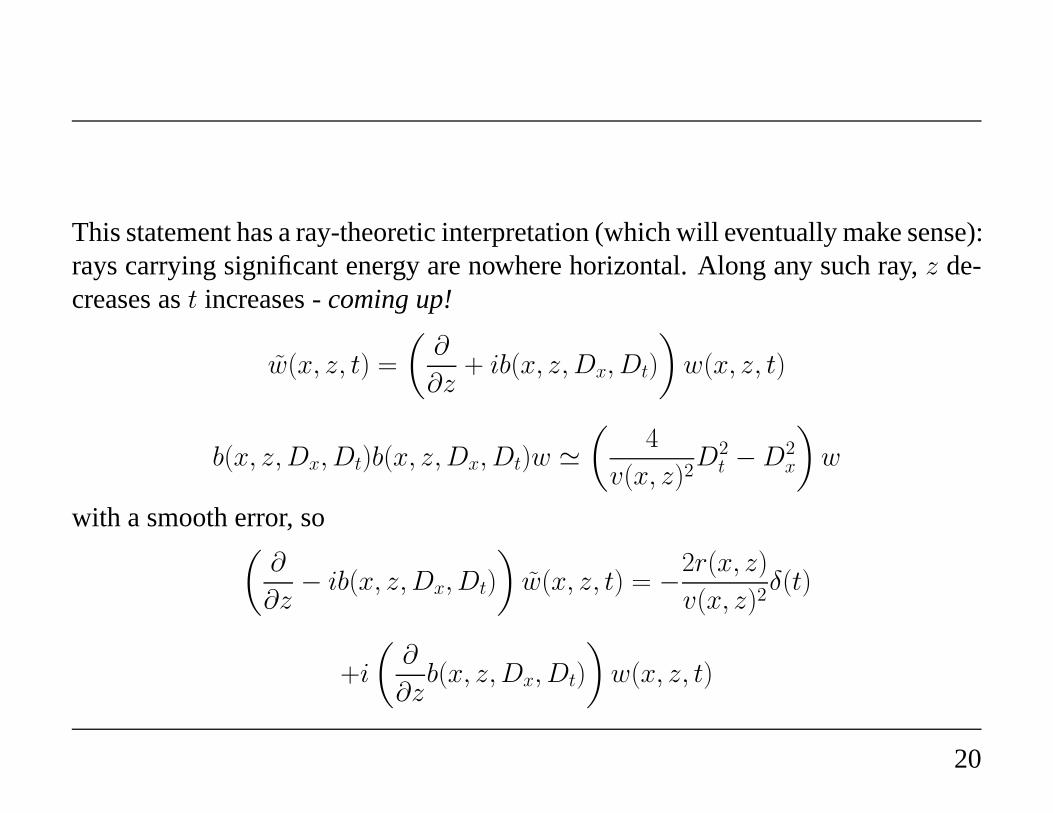
This statement has a ray-theoretic interpretation (which will eventually make sense):rays carrying significant energy are nowhere horizontal. Along any such ray,z de-creases ast increases -coming up!
w(x, z, t) =
(
∂
∂z+ ib(x, z, Dx, Dt)
)
w(x, z, t)
b(x, z,Dx, Dt)b(x, z,Dx, Dt)w ≃
(
4
v(x, z)2D2
t − D2x
)
w
with a smooth error, so(
∂
∂z− ib(x, z,Dx, Dt)
)
w(x, z, t) = −2r(x, z)
v(x, z)2δ(t)
+i
(
∂
∂zb(x, z,Dx, Dt)
)
w(x, z, t)
20

(sinceb depends onz, thez deriv. does not commute withb). So w = w0 + w1,where
(
∂
∂z− ib(x, z,Dx, Dt)
)
w0(x, z, t) = −2r(x, z)
v(x, z)2δ(t)
(this is theSSR modeling equation)
(
∂
∂z− ib(x, z,Dx, Dt)
)
w1(x, z, t) = i
(
∂
∂zb(x, z,Dx, Dt)
)
w(x, z, t)
Claim: WF (w1) ⊂ WF (w). Granted this⇒ WF (w0) ⊂ WF (w) also.
21

Upshot: SSR modeling
F0[v]r(xs, zs, t) = w0(xs, zs, t)
produces the same singularities (i.e. the same waves) as exploding reflector model-ing, so is as good a basis for migration.
SSR migration: assume that sources all lie onzs = 0.
< F0[v]∗d, r >=< d, F0[v]r >
=
∫
dxs
∫
dt d(xs, t)w0(xs, 0, t)
22

=
∫
dxs
∫
dt
∫
dz ¯d(xs, t)δ(z)w0(xs, z, t)
Define the adjoint fieldq by(
∂
∂z− b(x, z,Dx, Dt)
)
q(x, z, t) = d(x, t)δ(z), q(x, z, t) ≡ 0, z < 0
which is equivalent to solving the initial value problem(
∂
∂z− ib(x, z,Dx, Dt)
)
q(x, z, t) = 0, z > 0; , q(x, 0, t) = d(x, t)
Insert in expression for inner product, integrate by parts,use self-adjointness ofb,get
< d, F0[v]r >=
∫
dx
∫
dz2r(x, z)
v(x, z)2q(x, z, 0)
23

whence
F0[v]∗d(x, z) =2
v(x, z)2q(x, z, 0)
Standard description of the SSR migration algorithm:
• downward continue data (i.e. solve forq)
• image att = 0.
The art of SSR migration: computable approximations tob(x, z, Dx, Dt) - swim-ming pool operator, many successors.
24

Proof of the Claim
Unfinished business: proof of claim
Depends on celebratedPropagation of Singularities theorem of Hormander (1970).
Given symbolp(x, ξ), order m, with asymptotic expansion, definebicharateristicsas solutions(x(t), ξ(t)) of Hamiltonian system
dx
dt=
∂p
∂ξ(x, ξ),
dξ
dt= −
∂p
∂x(x, ξ)
with p(x(t), ξ(t)) ≡ 0.
Theorem: Supposep(x, D)u = f , and suppose that fort0 ≤ t ≤ t1, (x(t), ξ(t)) /∈
WF (f). Then either(x(t), ξ(t)) : t0 ≤ t ≤ t1 ⊂ WF (u) or (x(t), ξ(t)) : t0 ≤
t ≤ t1 ⊂ T ∗(Rn) − WF (u).
25
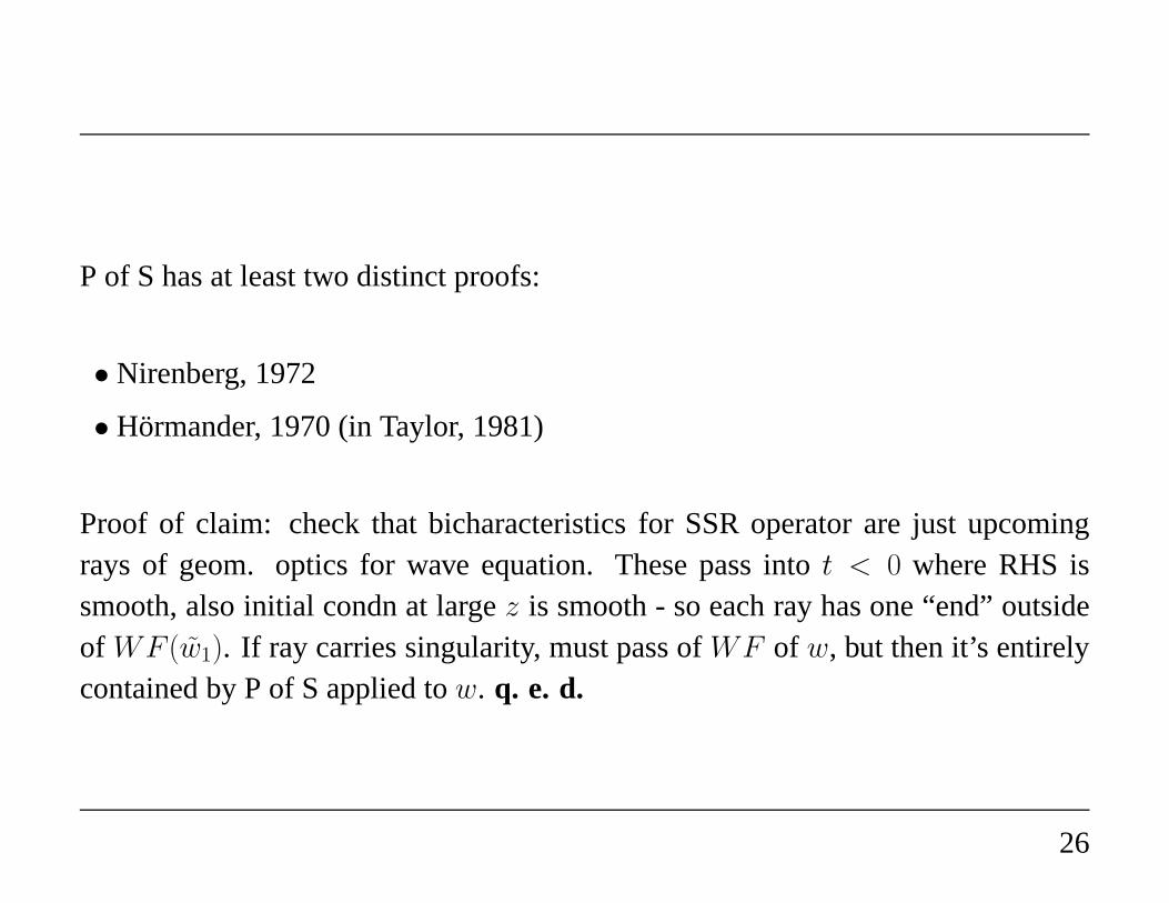
P of S has at least two distinct proofs:
• Nirenberg, 1972
• Hormander, 1970 (in Taylor, 1981)
Proof of claim: check that bicharacteristics for SSR operator are just upcomingrays of geom. optics for wave equation. These pass intot < 0 where RHS issmooth, also initial condn at largez is smooth - so each ray has one “end” outsideof WF (w1). If ray carries singularity, must pass ofWF of w, but then it’s entirelycontained by P of S applied tow. q. e. d.
26

Reverse Depth Migration, Prestack
Nonzero offset (“prestack”): starting point is integral representation of the scatteredfield
F [v]r(xr, t;xs) =∂2
∂t2
∫
dx2r(x)
v(x)2
∫
dsG(xr, t − s;x)G(xs, s;x)
By analogy with zero offset case, would like to view this as “exploding reflectorsin both directions”: reflectors propagate energy upward to sources and to receivers.
However can’t do this because reflection location issamefor both.
27
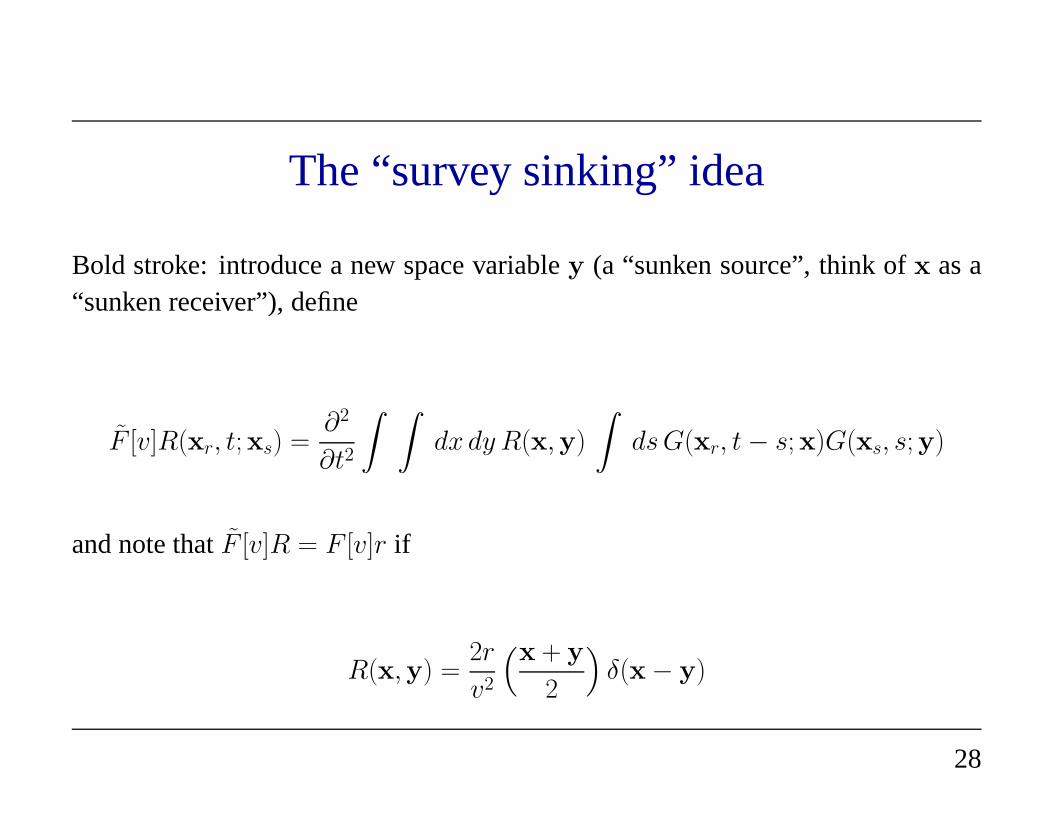
The “survey sinking” idea
Bold stroke: introduce a new space variabley (a “sunken source”, think ofx as a“sunken receiver”), define
F [v]R(xr, t;xs) =∂2
∂t2
∫ ∫
dx dy R(x,y)
∫
dsG(xr, t − s;x)G(xs, s;y)
and note thatF [v]R = F [v]r if
R(x,y) =2r
v2
(
x + y
2
)
δ(x − y)
28

This trick decomposesF [v] into two “exploding reflectors”:
F [v]R(xr, t;xs) = u(x, t;xs)|x=xr
where(
1
v(x)2∂2
∂t2−∇2
x
)
u(x, t;xs) =
∫
dy R(x,y)G(xs, t;y)
≡ ws(xs, t;x)
(“upward continue the receivers”),(
1
v(y)2∂2
∂t2−∇2
y
)
ws(y, t;x) = R(x,y)δ(t)
(“upward continue the sources”).
29
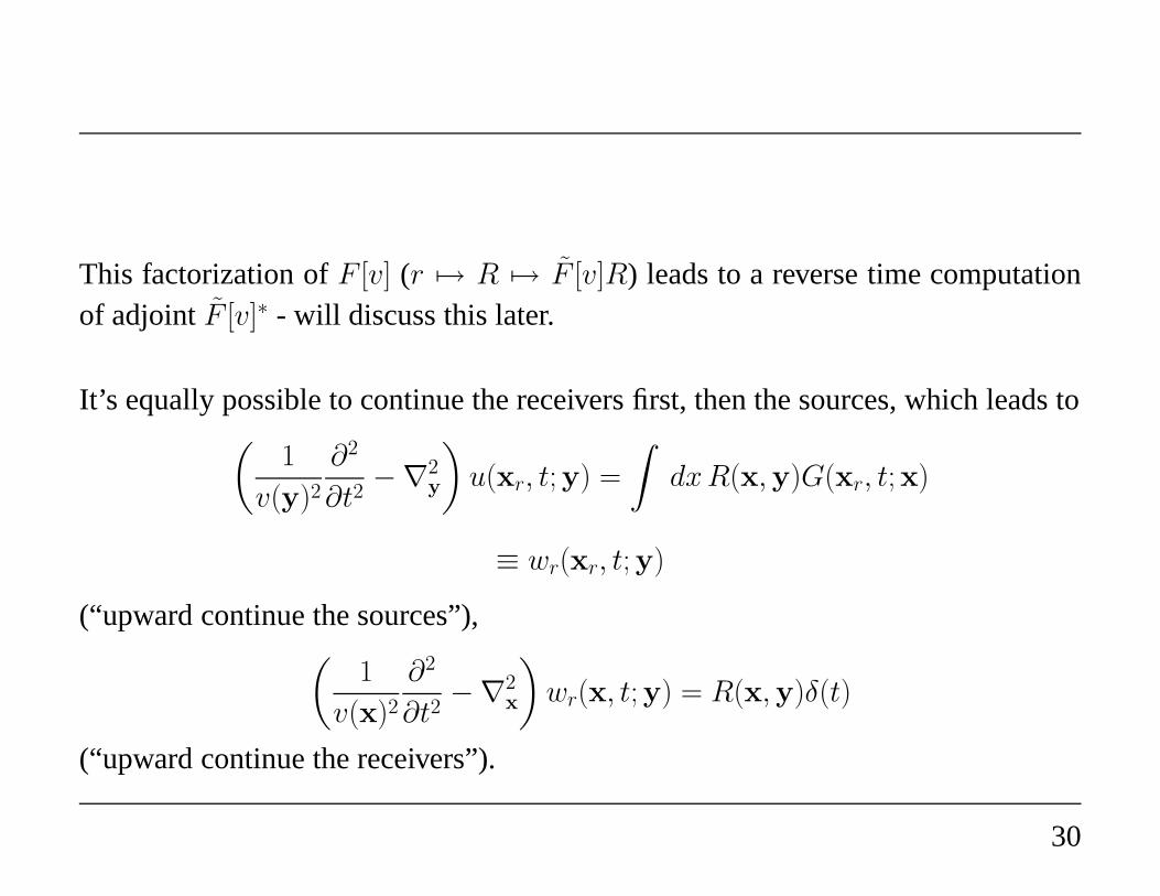
This factorization ofF [v] (r 7→ R 7→ F [v]R) leads to a reverse time computationof adjointF [v]∗ - will discuss this later.
It’s equally possible to continue the receivers first, then the sources, which leads to(
1
v(y)2∂2
∂t2−∇2
y
)
u(xr, t;y) =
∫
dxR(x,y)G(xr, t;x)
≡ wr(xr, t;y)
(“upward continue the sources”),(
1
v(x)2∂2
∂t2−∇2
x
)
wr(x, t;y) = R(x,y)δ(t)
(“upward continue the receivers”).
30

The DSR Assumption
Apply reverse depth concept: as before, go 2D temporarily,x = (x, zr),y = (y, zs),all sources and receivers onz = 0.
Double Square Root (“DSR”) assumption: For someδ > 0, the wavefieldu satis-fies
(x, zr, t, y, zs, ξ, ζs, τ, η, ζr) ∈ WF (u) ⇒
(x, t, ξ, τ ) ∈ Pδ(zr), (y, t, η, τ ) ∈ Pδ(zs), andζrτ > 0, ζsτ > 0,
As for SSR, there is a ray-theoretic interpretation: rays from source and receiver toscattering point stay away from the vertical and decrease inz for increasingt, i.e.they are all upcoming.
31
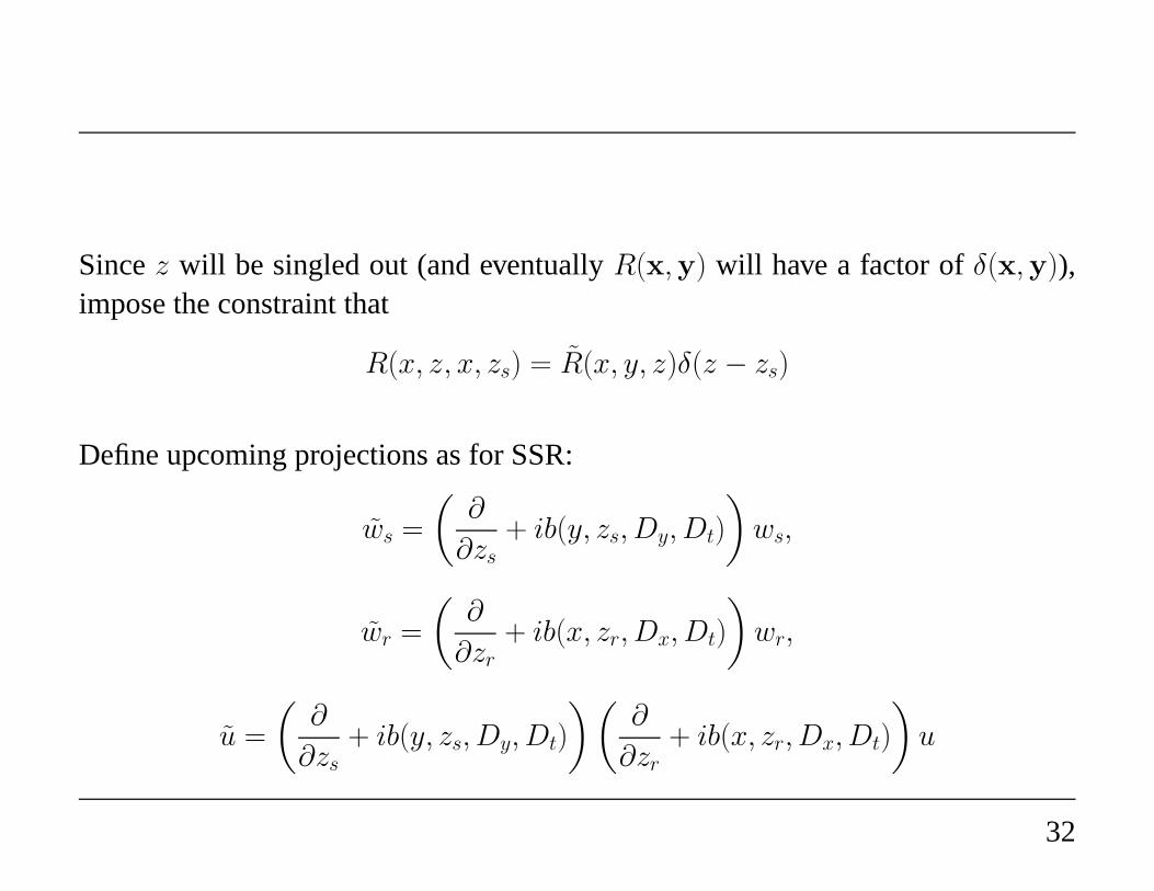
Sincez will be singled out (and eventuallyR(x,y) will have a factor ofδ(x,y)),impose the constraint that
R(x, z, x, zs) = R(x, y, z)δ(z − zs)
Define upcoming projections as for SSR:
ws =
(
∂
∂zs+ ib(y, zs, Dy, Dt)
)
ws,
wr =
(
∂
∂zr+ ib(x, zr, Dx, Dt)
)
wr,
u =
(
∂
∂zs+ ib(y, zs, Dy, Dt)
) (
∂
∂zr+ ib(x, zr, Dx, Dt)
)
u
32

Except for lower order commutators which we justify throwing away as before,(
∂
∂zs− ib(y, zs, Dy, Dt)
)
ws = Rδ(zr − zs)δ(t),
(
∂
∂zr− ib(x, zr, Dx, Dt)
)
wr = Rδ(zr − zs)δ(t),
(
∂
∂zr− ib(x, zr, Dx, Dt)
)
u = ws
(
∂
∂zs− ib(y, zs, Dy, Dt)
)
u = wr
Initial (final) conditions are thatwr, ws, andu all vanish for largez - the equationsare to be solve in decreasingz (“upward continuation”).
33

Simultaneous upward continuation:
∂
∂zu(x, z, t; y, z) =
∂
∂zru(x, zr, t; y, z)|z=zr +
∂
∂zru(x, z, t; y, zs)|z=zs
= [ib(x, zr, Dx, Dt)u + ws + ib(y, zs, Dy, Dt)u + wr]zr=zs=z
Sincews(y, z, t; x, z) = wr(x, z, t; y, z) = R(x, y, z)δ(t), u is seen to satisfy the
DSR modeling equation:(
∂
∂z− ib(x, z,Dx, Dt) − ib(y, z, Dy, Dt)
)
u(x, z, t; y, z) = 2R(x, y, z)δ(t)
F [v]R(xr, t; xs) = u(xr, 0, t; xs, 0)
34

DSR Migration
Computation of adjoint follows same pattern as for SSR, and leads to
DSR migration equation: solve(
∂
∂z− ib(x, z, Dx, Dt) − ib(y, z, Dy, Dt)
)
q(x, y, z, t) = 0
in increasingz with initial condition atz = 0:
q(xr, xs, 0, t) = d(xr, xs, t)
ThenF [v]∗d(x, y, z) = q(x, y, z, 0)
The physical DSR model hasR(x, y, z) = r(x, z)δ(x − y), so final step in DSRcomputation ofF [v]∗ is adjoint ofr 7→ R:
F [v]∗d(x, z) = q(x, x, z, 0)
35

Standard description of DSR migration
(See Claerbout, IEI):
• downward continue sources and receivers (solve DSR migration equation)
• image att = 0 and zero offset (x = y)
Another moniker: “survey sinking”: DSR fieldq is (related to) the field that youwould get by conducting the survey with sources and receivers at depthz. At anygiven depth, the zero-offset, time-zero part of the field is the instantaneous responseto scatterers on which source = receiver is sitting, therefore constitutes an image.
As for SSR, the art of DSR migration is in the approximation ofthe DSR operator.
36

Remarks
Stolk and deHoop (2001) derived DSR modeling and migration via a more system-atic argument than that used here, involvingΨDO matrix factorization of the waveequation written as a first order evolution system inz. This idea goes back to Tay-lor (1975) who used it to show that singularities propagating along bicharacteristicsreflect as expected at boundaries.
Stolk (2003) has also carried out a very careful global construction of a family ofSSRΨDOs which are of non-classical type at near-horizontal directions (“nearlyevanescent waves”). This construction should lead to more reliable discretizations.
The last part of the course will present the various apparently ad-hoc “prestackmodeling” ideas within a unified framework.
37

Mathematics of Seismic ImagingPart III
William W. Symes
PIMS, July 2005

A step beyond linearization: velocity analysis
1
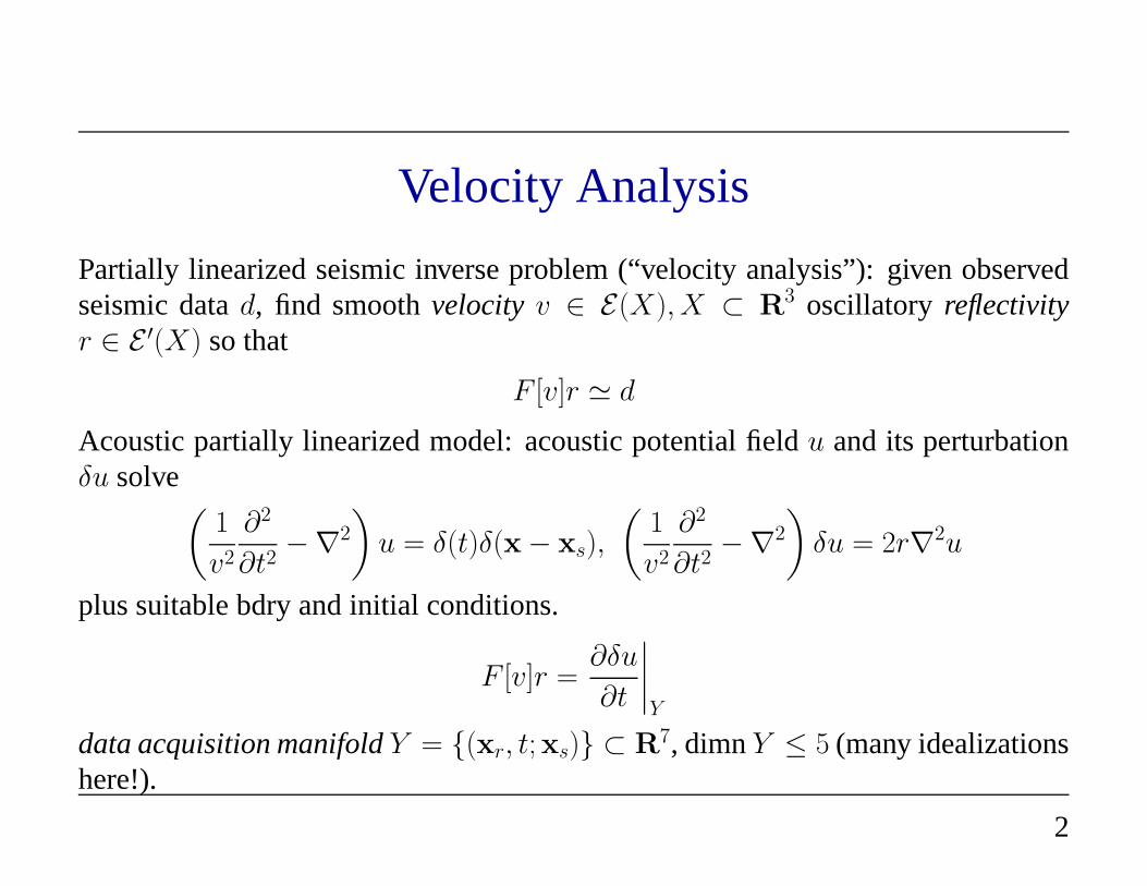
Velocity Analysis
Partially linearized seismic inverse problem (“velocity analysis”): given observedseismic datad, find smoothvelocity v ∈ E(X), X ⊂ R
3 oscillatory reflectivityr ∈ E ′(X) so that
F [v]r ≃ d
Acoustic partially linearized model: acoustic potential field u and its perturbationδu solve
(
1
v2
∂2
∂t2−∇2
)
u = δ(t)δ(x − xs),
(
1
v2
∂2
∂t2−∇2
)
δu = 2r∇2u
plus suitable bdry and initial conditions.
F [v]r =∂δu
∂t
∣
∣
∣
∣
Y
data acquisition manifoldY = (xr, t;xs) ⊂ R7, dimnY ≤ 5 (many idealizations
here!).
2

F [v] : E ′(X) → D′(Y ) is a linear map (FIO of order1), but dependence onv isquite nonlinear, so this inverse problem is nonlinear.
Agenda:
• reformulation of inverse problem viaextensions
• “standard processing” extension and standard VA
• the surface oriented extension and standard MVA
• theΨDO property and why it’s important
• global failure of theΨDO property for the SOE
• Claerbout’s depth oriented extension has theΨDO property
• differential semblance
3

Extensions
Extensionof F [v]: manifold X and mapsχ : E ′(X) → E ′(X), F [v] : E ′(X) →D′(Y ) so that
F [v]E ′(X) → D′(Y )
χ ↑ ↑ idE ′(X) → D′(Y )
F [v]
commutes.
Invertible extension:F [v] has aright parametrixG[v], i.e. I − F [v]G[v] is smooth-ing. [The trivial extension -X = X, F = F - is virtually never invertible.] Alsoχhas aleft inverseη.
Reformulation of inverse problem: givend, find v so thatG[v]d ∈ R(χ) (implicitlydeterminesr also!).
4
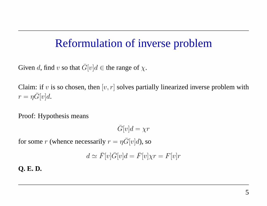
Reformulation of inverse problem
Givend, find v so thatG[v]d ∈ the range ofχ.
Claim: if v is so chosen, then[v, r] solves partially linearized inverse problem withr = ηG[v]d.
Proof: Hypothesis means
G[v]d = χr
for somer (whence necessarilyr = ηG[v]d), so
d ≃ F [v]G[v]d = F [v]χr = F [v]r
Q. E. D.
5
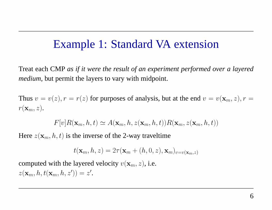
Example 1: Standard VA extension
Treat each CMPas if it were the result of an experiment performed over a layeredmedium, but permit the layers to vary with midpoint.
Thusv = v(z), r = r(z) for purposes of analysis, but at the endv = v(xm, z), r =
r(xm, z).
F [v]R(xm, h, t) ≃ A(xm, h, z(xm, h, t))R(xm, z(xm, h, t))
Herez(xm, h, t) is the inverse of the 2-way traveltime
t(xm, h, z) = 2τ (xm + (h, 0, z),xm)v=v(xm,z)
computed with the layered velocityv(xm, z), i.e.z(xm, h, t(xm, h, z′)) = z′.
6
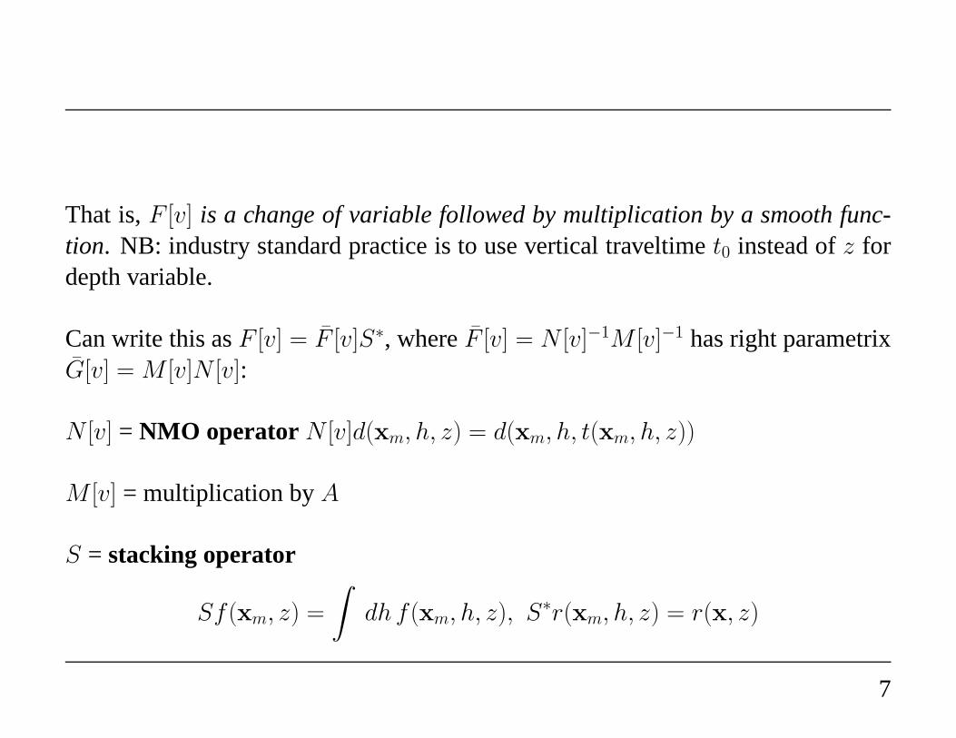
That is,F [v] is a change of variable followed by multiplication by a smooth func-tion. NB: industry standard practice is to use vertical traveltime t0 instead ofz fordepth variable.
Can write this asF [v] = F [v]S∗, whereF [v] = N [v]−1M [v]−1 has right parametrixG[v] = M [v]N [v]:
N [v] = NMO operator N [v]d(xm, h, z) = d(xm, h, t(xm, h, z))
M [v] = multiplication byA
S = stacking operator
Sf(xm, z) =
∫
dh f(xm, h, z), S∗r(xm, h, z) = r(x, z)
7

Identify as extension:F [v], G[v] as above,X = xm, z, H = h, X = X ×
H,χ = S∗, η = S - the invertible extension properties are clear.
Standard names for the Standard VA extension objects:F [v] = “inverse NMO”,G[v] = “NMO” [often the multiplication opM [v] is neglected];η = “stack”, χ =“spread”
How this is used for velocity analysis: Look for v that makesG[v]d ∈ R(χ)
So what isR(χ)? χ[r](xm, z, h) = r(xm, z) Anything in range ofχ is independentof h. Practical issues⇒ replace “independent of” with “smooth in”.
8

Flatten them gathers!
Inverse problem reduced to: adjustv to makeG[v]dobs smooth inh, i.e. flat in z, h
display for eachxm (NMO-corrected CMP).
Replacez with t0, v with vRMS em localizes computation: reflection throughxm, t0, 0
flattenedby adjustingvRMS(xm, t0) ⇒ 1D search, do by visual inspection.
Various aids - NMO corrected CMP gathers, velocity spectra,etc.
See: Claerbout:Imaging the Earth’s Interior
WWS: MGSS 2000 notes
9

0.6
0.8
1.0
1.2
1.4
1.6
1.8
time
(s)
10 20 30 40 50channel
,
0
0.5
1.0
1.5
2.0
time
(s)
0.5 1.0 1.5 2.0 2.5offset (km)
Left: part of survey (d) from North Sea (thanks: Shell Research), lightly prepro-cessed.Right: restriction ofG[v]d to xm = const (function of depth, offset): shows rel.sm’ness inh (offset) for properly chosenv.
10

Example 2: Surface oriented or standard MVA
extension
. Standard VA only works where Earth is “nearly layered”. Where this fails, replaceNMO by prestack migration.
Version based on common offset modeling/migration:Σh = set of half-offsets indata,X = X × Σh, χ[r](x,h) = r(x).
F [v]r(xs, t,h) =∂2
∂t2
∫
dx r(x,h)
∫
dsG(xs + 2h, t − s;x)G(xs, s; x)
Note that this operator is “block diagonal” inh.
11

Properties of SOE
Beylkin (1985), Rakesh (1988): if‖v‖C2(X) “not too big”, then
• F hasthe ΨDO property: F F ∗ is ΨDO
• singularities ofF F ∗d ⊂ singularities ofd
• straightforward construction of right parametrixG = F ∗Q, Q = ΨDO, also asgeneralized Radon Transform - explicitly computable.
Range ofχ (offset version):r(x,h) independent ofh ⇒ “semblance principle”:find v so thatG[v]dobs is independent ofh. Practical limitations⇒ replace “inde-pendent ofh” by “smooth inh”.
12

Industrial MVA
Application of these ideas = industrial practice of migration velocity analysis.
Idea: twiddlev until G[v]dobs is smooth inh.
Since it is hard to inspectG[v]dobs(x, y, z, h), pull out subset for constantx, y =common image gather (“CIG”): display function ofz, h for fixedx, y. These playsame role as NMO corrected CMP gathers in layered case.
Try to adjustv so that selected CIGs areflat - just as in Standard VA. This is muchharder, as there is no RMS velocity trick to localize the computation - each CIGdepends globally onv.
Description, some examples: Yilmaz,Seismic Data Processing.
13

Bad news
Nolan (1997), Stolk & WWS (2004): big trouble! In general, standard extensiondoesnot have theΨDO property. Geometric optics analysis: for‖v‖C2(X) “large”,multiple rays connect source, receiver to reflecting pointsin X; block diagonalstructure ofF [v] ⇒ info necessary to distinguish multiple rays isprojected out.
14

2
1
0
x2
-1 0 1x1
1
0.6
Example (Stolk & WWS, 2001): Gaussian lens over flat reflectorat depth z (r(x) =
δ(x1 − z), x1 = depth).
15

1.6
2.0
2.4
x2
0.0 0.4 0.8x1
,
1.6
2.0
2.4
x2
0 1 2offset
3,2
3,1
1,2
2,1
3,3
1,1
travel time # s,r
Left: Const.h slice of Gd: several refl. points corresponding to same singularityin dobs.Right: CIG (const.x, y slice) ofGd: not smooth inh!
16

Example 3: Claerbout’s depth oriented extension
Standard MVA extension only works when Earth has simple ray geometry. Claer-bout (1971) proposed alternative extension:
Σd = somewhat arbitrary set of vectors near 0 (“offsets”),X = X×Σd, χ[r](x,h) =
r(x)δ(h), η[r](x) = r(x, 0)
F [v]r(xs, t,xr) =∂2
∂t2
∫
dx
∫
Σd
dh r(x,h)
∫
dsG(xs, t − s;x + 2h)G(xr, s;x)
=∂2
∂t2
∫
dx
∫
x+2Σd
dy r(x,y − x)
∫
dsG(xs, t − s;y)G(xr, s;x)
NB: in this formulation, there appears to be too many model parameters.
17

Shot record modeling
for eachxs solve
F [v]r(xr, t;xs) = u(x, t;xs)|x=xr
where(
1
v(x)2∂2
∂t2−∇2
x
)
u(x, t;xs) =
∫
x+2Σd
dy r(x,y)G(y, t;xs)
(
1
v(y)2∂2
∂t2−∇2
y
)
G(y, t;xs) = δ(t)δ(xs − y)
Finite difference scheme: form RHS for eqn 1, stepu, G forward in t.
18

ComputingG[v]
Instead of parametrix, be satisfied with adjoint.
Reverse time adjoint computation - specify adjoint field as in standard reverse timeprestack migration:
(
1
v(x)2∂2
∂t2−∇2
x
)
w(x, t;xs) =
∫
dxr d(xr, t;xs)δ(x − xr)
with w(x, t;xs) = 0, t >> 0. Then
F [v]∗d(x,h) =
∫
dxs
∫
dtG(x + 2h, t;xs)w(x, t;xs)
i.e. exactly the same computation as for reverse time prestack, except that crosscor-relation occurs at an offset2h.
19
Nomenclature
NB: the “usual computation” ofG[v] is either DSR or a variant of shot record com-putation of previous slide using depth extrapolation.h is usually restricted to behorizontal, i.e.h3 = 0.
Common names: shot-geophone or survey-sinking migration (with DSR), or shotrecord migration.
“Downward continue sources and receivers, image att = 0, h = 0”
These are what is typically meant by “wave equation migration”!
20

What should be the character of the image when the velocity iscorrect?
Hint: for simulation of seismograms, the input reflectivityhad the formr(x)δ(h).
Therefore guess that when velocity is correct,image is concentrated nearh = 0.
Examples: 2D finite difference implementation of reverse time method. Correctvelocity ≡ 1. Input reflectivity used to generate synthetic data: random! Foroutput reflectivity (image ofF [v]∗), constrain offset to be horizontal:r(x,h) =
r(x, h1)δ(h3). Display CIGs (i.e.x1 =const. slices).
21

0
0.1
0.2
0.3
0.4
0.5
depth
(km
)
-0.2 -0.1 0 0.1offset (km)
Offset Image Gather, x=1 km
,
0
0.1
0.2
0.3
0.4
0.5
depth
(km
)
-0.2 -0.1 0 0.1offset (km)
OIG, x=1 km: vel 10% high
,
0
0.1
0.2
0.3
0.4
0.5
depth
(km
)
-0.2 -0.1 0 0.1offset (km)
OIG, x=1 km: vel 10% low
Two way reverse time horizontal offset S-G image gathers of data from randomreflectivity, constant velocity. From left to right: correct velocity, 10% high, 10%low.
22

Stolk and deHoop, 2001
Claerbout extension has theΨDO property, at least when restricted tor of the formr(x,h) = R(x, h1, h2)δ(h3), and under DSR assumption.
Sketch of proof (after Rakesh, 1988):
This will follow from injectivityof wavefront orcanonical relationCF ⊂ T ∗(X)−
0 × T ∗(Y ) − 0 which describes singularity mapping properties ofF :
(x,h, ξ, ν,y, η) ∈ CFδ[v] ⇔
for someu ∈ E ′(X), (x,h, ξ, ν) ∈ WF (u), and (y, η) ∈ WF (F u)
23
Characterization ofCF
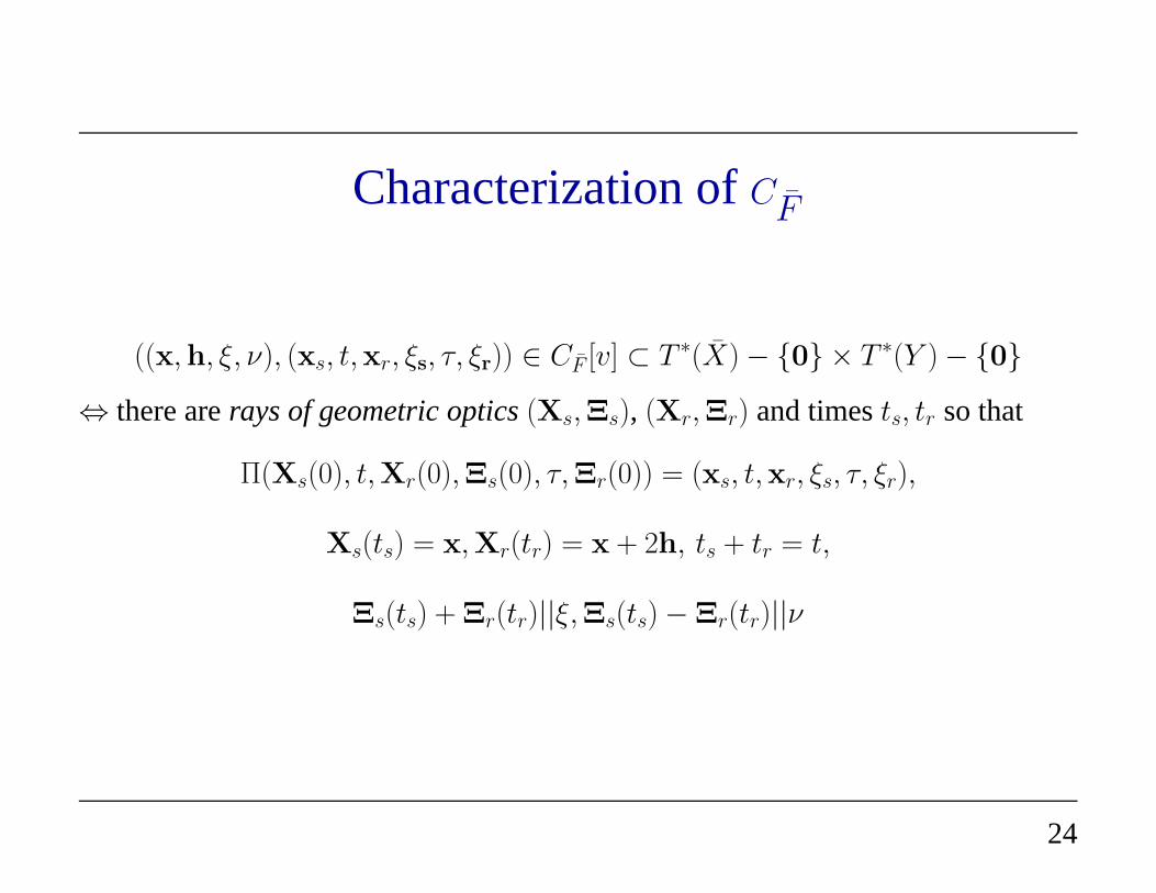
((x,h, ξ, ν), (xs, t,xr, ξs, τ, ξr)) ∈ CF [v] ⊂ T ∗(X) − 0 × T ∗(Y ) − 0
⇔ there arerays of geometric optics(Xs,Ξs), (Xr,Ξr) and timests, tr so that
Π(Xs(0), t,Xr(0),Ξs(0), τ,Ξr(0)) = (xs, t,xr, ξs, τ, ξr),
Xs(ts) = x,Xr(tr) = x + 2h, ts + tr = t,
Ξs(ts) + Ξr(tr)||ξ,Ξs(ts) − Ξr(tr)||ν
24

ξ,
Π Π
ξ
(t )r r
(t )r r
s(t )s (t )ss
ss ss(t’ ) (t’ )
r rr (t’ ) (t’ )
t + t = t’ + t’s s r,r,
r
x s, s x r, rp
x
p
kx x k
kxk
25

Proof
Uses wave equations foru, G and
• Gabor calculus: computes wave front sets of products, pullbacks, integrals, etc.See Duistermaat, Ch. 1.
• Propagation of Singularities Theorem
and that’s all! [No integral representations, phase functions,...]
26

Note intrinsic ambiguity: if you have a ray pair, move timests, tr resp. t′s, t′r, for
whichts+tr = t′s+t′r = t then you can construct two points(x,h, ξ, ν), (x′,h′, ξ′, ν ′)
which are candidates for membership inWF (r) and which satisfy the above rela-tions with the same point in the cotangent bundle ofT ∗(Y ).
No wonder - there are too many model parameters!
Stolk and deHoop fix this ambiguity by imposing two constraints:
• DSR assumption: all rays carrying significant reflected energy (source or re-ceiver) are upcoming.
• RestrictF to the domainZ ⊂ E ′(X)
r ∈ Z ⇔ r(x,h) = R(x, h1, h2)δ(h3)
27

If r ∈ Z, then(x,h, ξ, ν) ∈ WF (r) ⇒ h3 = 0. So source and receiver rays inCF
must terminate at same depth, to hit such a point.
Because of DSR assumption, this fixes the traveltimests, tr.
Restricted to Z , CF is injective.
⇒ CF ∗F = I
⇒ F ∗F is ΨDO when restricted toZ.
28

xr(t )
r r(t )
r
s ,p
s(t )s(t )sx s
x r, rx s,,p
k k
29

Lens data, shot-geophone migration [B. Biondi, 2002]Left: Image via DSR. Middle:G[v]d - well-focused (ath = 0), i.e. in range ofχ to
extent possible. Right: Angle CIG.
30

Quantitative VA
SupposeW : E ′(X) → D′(Z) annihilates range ofχ:
χ WE ′(X) → E ′(X) → D′(Z) → 0
and moreoverW is bounded onL2(X). Then
J [v; d] =1
2‖WG[v]d‖2
minimizedwhen[v, ηG[v]d] solves partially linearized inverse problem.
Construction ofannihilatorof R(F [v]) (Guillemin, 1985):
d ∈ R(F [v]) ⇔ G[v]d ∈ R(χ) ⇔ WG[v]d = 0
31
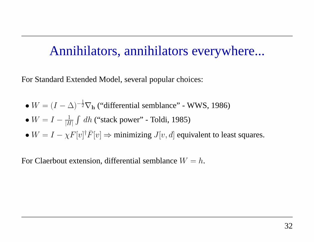
Annihilators, annihilators everywhere...
For Standard Extended Model, several popular choices:
• W = (I − ∆)−12∇h (“differential semblance” - WWS, 1986)
• W = I − 1|H|
∫
dh (“stack power” - Toldi, 1985)
• W = I − χF [v]†F [v] ⇒ minimizingJ [v, d] equivalent to least squares.
For Claerbout extension, differential semblanceW = h.
32
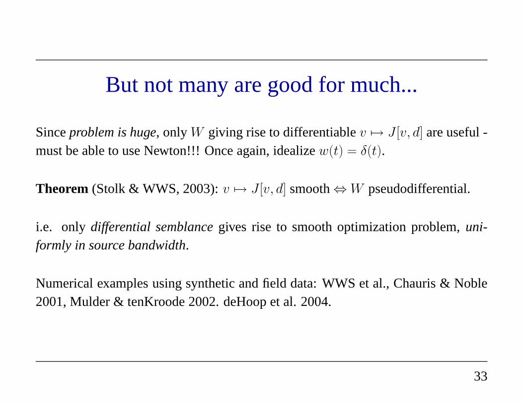
But not many are good for much...
Sinceproblem is huge, only W giving rise to differentiablev 7→ J [v, d] are useful -must be able to use Newton!!! Once again, idealizew(t) = δ(t).
Theorem (Stolk & WWS, 2003):v 7→ J [v, d] smooth⇔ W pseudodifferential.
i.e. only differential semblancegives rise to smooth optimization problem,uni-formly in source bandwidth.
Numerical examples using synthetic and field data: WWS et al., Chauris & Noble2001, Mulder & tenKroode 2002. deHoop et al. 2004.
33
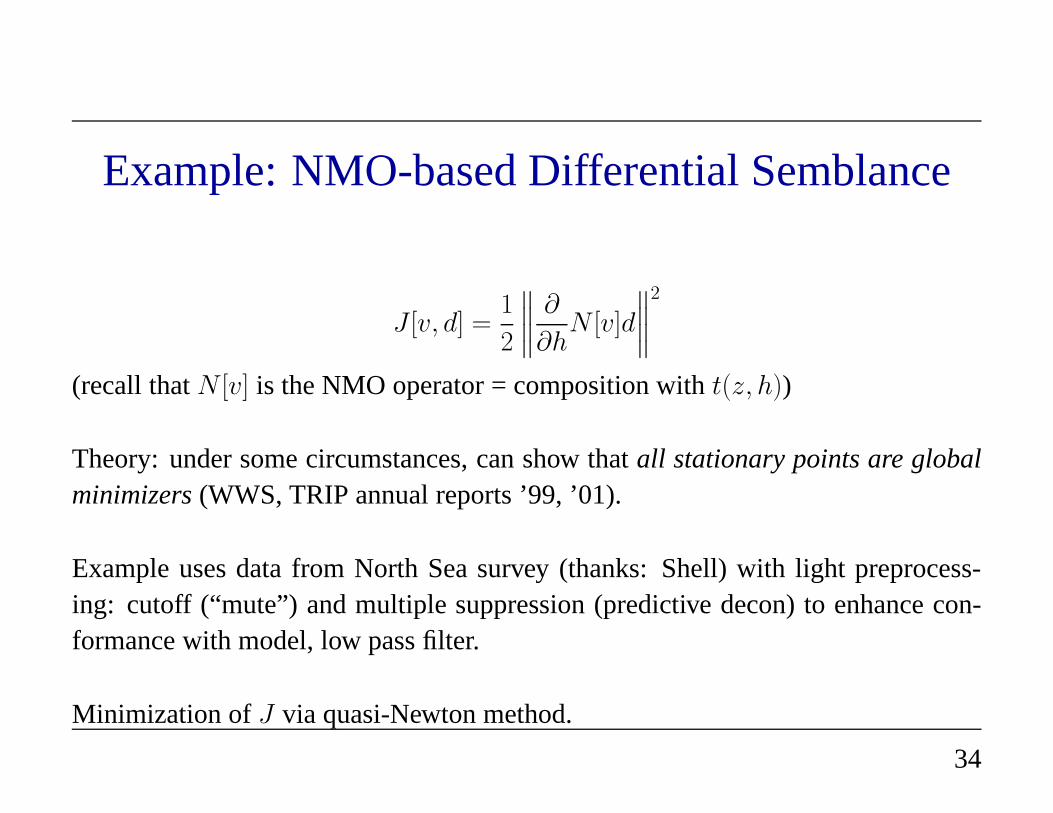
Example: NMO-based Differential Semblance
J [v, d] =1
2
∥
∥
∥
∥
∂
∂hN [v]d
∥
∥
∥
∥
2
(recall thatN [v] is the NMO operator = composition witht(z, h))
Theory: under some circumstances, can show thatall stationary points are globalminimizers(WWS, TRIP annual reports ’99, ’01).
Example uses data from North Sea survey (thanks: Shell) withlight preprocess-ing: cutoff (“mute”) and multiple suppression (predictivedecon) to enhance con-formance with model, low pass filter.
Minimization ofJ via quasi-Newton method.
34
Beyond Born
Nonlinear effects not included in linearized model:multiple reflections. Conven-tional approach: treat ascoherent noise, attempt to eliminate - active area of re-search going back 40+ years, with recent important developments.
Why not model this “noise”?
Proposal:nonlinear extensionswith F [v]r replaced byF [c]. Create annihilators insame way (now also nonlinear), optimize differential semblance.
Nonlinear analog of Standard Extended Model appears to beinvertible - in factextended nonlinear inverse problem isunderdetermined.
Open problems: no theory. Also must determinew(t) (Lailly SEG 2003).
35

And so on...
• Elasticity: theory of asymptotic Born inversion at smooth background in goodshape (Beylkin & Burridge 1988, deHoop & Bleistein 1997). Theory of exten-sions, annihilators, differential semblance partially complete (Brandsberg-Dahlet al 2003).
• Anisotropy - work of deHoop (Brandsberg-Dahl et al 2003).
• Anelasticity - in the sedimentary section,Q = 100 − 1000, lower in gassy sedi-ments and near surface. No mathematical results, but some numerics - Minkoff& WWS 1997, Blanch et al 1998.
• Source determination - actually always an issue. Some success in casting as aninverse problem - Minkoff & WWS 1997, Routh et al SEG 2003.
• ...
36

Mathematics of Seismic Imaging:Selected References
William W. Symes
July 2005

Overviews
Bleistein, N., Cohen, J. and Stockwell, J.:The Mathematics of Seismic Imaging,Migration, and Inversion, Springer, 2000.
Symes, W. W.:Mathematics of Reflection Seismology, Lecture Notes,www.trip.caam.rice.edu, 1995.
1

Imaging (1)
Cohen, J. K. and Bleistein, N.: An inverse method for determining small variationsin propagation speed,SIAM J. Appl. Math. 32, 1977, pp. 784-799.
Beylkin, G.: Imaging of discontinuities in the inverse scattering problem by inver-sion of a causal generalized Radon transform,J. Math. Phys 26, 1985, pp. 99-108.
Miller, D., Oristaglio,, M. and Beylkin, G.: A new slant on seismic imaging,Geo-physics 52, pp. 943-964, 1987.
Rakesh: A linearized inverse problem for the wave equation,Comm. PDE 13, 1988,pp. 573-601.
Ten Kroode, A. P. E., Smit, D. J., and Verdel, A. R.: A microlocal analysis ofmigrationWave Motion 28, 1998, pp. 149-172.
2

Imaging (2)
Nolan, C. J. and Symes, W. W.: Global solution of a linearizedinverse problem forthe wave equation,Comm. PDE 22, 1997, pp. 919-952.
deHoop, M. and Bleistein, N.: Generalized Radon Transform inversions for reflec-tivity in anisotropic elastic media,Inverse Problems 16, 1998, pp. 669-690.
Stolk, C.: Microlocal analysis of a seismic linearized inverse problem,Wave Motion32, 2000, pp. 267-290.
Operto, S., Xu, S. and Lambare, G.: Can we image quantitatively complex modelswith rays?,Geophysics 65, 2001, pp. 1223-1238.
Stolk, C. and Symes, W. W.: Kinematic artifacts in prestack depth migration,Geo-physics 68, May-June 2004.
3

Velocities
Minkoff, S. E. and Symes, W. W.: Full waveform inversion of marine reflectiondata in the plane wave domain,Geophysics 62, 1997, pp. 540-553.
Brandsberg-Dahl, S., De Hoop, M., and Ursin, B.: Focussing in dip and AVAcompensation on scattering angle/azimuth common image gathers,Geophysics 68,2003, pp. 232-254.
Stolk, C. and Symes, W. W.: Smooth objective functionals forseismic velocityinversion,Inverse Problems 19, 2003, pp. 73-89.
Stolk, C. and deHoop, M.: Seismic inverse scattering in the wave equation ap-proach, MSRI preprint, 2001.
Shen, P., Stolk, C. and Symes, W. W.: Differential semblancevelocity analysis bywave-equation migration, Expanded Abstracts, Society of Exploration Geophysi-cists 73rd Annual International Meeting and Exposition, pp. 2135-2139, 2003.
4
Mathematical Background
Lions, J. L.:Nonhomogeneous Boundary Value Problems and Applications, SpringerVerlag, Berlin, 1972.
Nirenberg, L.: Lectures on Partial Differential Equations, CMBS Lecture Notes,AMS, 1972.
Treves, F.:Introduction To Pseudodifferential Operators And FourierIntegral Op-erators, Plenum, 1980.
Duistermaat, J.:Fourier Integral Operators, Birkhauser, NY, 1996.
Taylor, M.: Pseudodifferential Operators, Princeton University Press, 1981.
Hormander, L.:The Analysis of Linear Partial Differential Operators, vols. I-IV,Springer Verlag, 1983.
5

Geophysical Classics
Hagedoorn, F.: A process of seismic reflection interpretation,Geophysical Prospect-ing, 1954, pp. 85-127.
Claerbout, J.:Basic Earth Imaging(“BEI”) and Imaging the Earth’s Interior(“IEI”),available through SEP web site,sepwww.stanford.edu.
Grau, G. and Versteeg, R.:The Marmousi Experience: Practical Aspects of Inver-sion, IFP-Technip, Paris, 1991.
Dobrin, M. and Savit, C.:Introduction to Geophysical Prospecting, 4th edition,McGraw-Hill, 1988.
Yilmaz, O.: Seismic Data Processing, 2nd edtion, SEG, 1999.
6