Math 320-3: Lecture NotesNorthwestern University, Spring 2015

Written by Santiago Canez

These are lecture notes for Math 320-3, the third quarter of “Real Analysis”, taught at North-western University in the spring of 2015. The book used was the 4th edition of An Introduction toAnalysis by Wade. Watch out for typos! Comments and suggestions are welcome.

Contents

March 30, 2015: Limits and Continuity 2

April 1, 2015: Linear Transformations, Partial Derivatives 5

April 3, 2015: Second-Order Partial Derivatives 9

April 6, 2015: Clairaut’s Theorem, Differentiability 13

April 8, 2015: More on Differentiability 18

April 10, 2015: Yet More on Derivatives 22

April 13, 2015: The Chain Rule 26

April 15, 2015: Mean Value Theorem 31

April 17, 2015: More on Mean Value, Taylor’s Theorem 35

April 20, 2015: Inverse Function Theorem 38

April 22, 2015: Implicit Function Theorem 43

April 24, 2015: More on Implicit Functions 46

April 27, 2015: Jordan Measurability 50

May 1, 2015: Riemann Integrability 56

May 4, 2015: More on Integrability 61

May 6, 2015: Fubini’s Theorem 65

May 8, 2015: Change of Variables 72

May 11, 2015: Curves 77

May 13, 2015: Surfaces 81

May 15, 2015: Orientations 86

May 18, 2015: Vector Line/Surface Integrals 91

May 22, 2015: Green’s Theorem 94

May 27, 2015: Stokes’ Theorem 98

May 29, 2015: Gauss’s Theorem 105

June 1, 2015: Differential Forms 109

March 30, 2015: Limits and Continuity

Welcome to the final quarter of real analysis! This quarter, to use an SAT-style analogy, is tomultivariable calculus what the first quarter was to single-variable calculus. That is, this quarteris all about making precise the various concepts you would see in a multivariable calculus course—such as multivariable derivatives and integrals, vector calculus and Stokes’ Theorem—and pushingthem further. After giving a broad introduction to this, we started talking about limits.

The Euclidean norm. First we clarify some notation we’ll be using all quarter long. The bookdiscusses this in Chapter 8, which is essentially a review of linear algebra.

For a point a ∈ Rn written in components as a = (a1, . . . , an), the (Euclidean) norm of a is

‖a‖ =√a2

1 + . . .+ a2n,

and is nothing but the usual notion of length when we think of a as a vector. Thus for a,b ∈ Rn,the norm of their difference:

‖a− b‖ =√

(a1 − b1)2 + · · ·+ (an − bn)2

is nothing but the Euclidean distance between a and b, so in the language of metrics from lastquarter we have

d(a,b) = ‖a− b‖

and ‖a‖ is then the distance from a to the origin 0. Using what we know about this Euclideandistance, we know that sometimes we can instead phrase things in terms of the taxicab or boxmetrics instead, but ‖·‖ will always denote Euclidean length.

Limits. Suppose that V ⊆ Rn is open and that a ∈ Rn. For a function f : V \a → Rm, we saythat the limit of f as x approaches a is L ∈ Rm if for all ε > 0 there exists δ > 0 such that

0 < ‖x− a‖ < δ implies ‖f(x)− L‖ < ε.

Limits are unique when they exist, and we use the notation limx→a

f(x) = L when this is the case.

The book discusses such limits in Chapter 9, which we skipped last quarter in favor of the metricspace material in Chapter 10. These notes should cover everything we’ll need to know about limits,but it won’t hurt to briefly glance over Chapter 9 on your own.

Remarks. A few remarks are in order. First, since the two norms used in the definitions are givingdistances in Rn and Rm respectively, it is clear that a similar definition works for metric spacesin general. Indeed, all we do is take the ordinary definition of a limit for single-variable functionsfrom first quarter analysis and replace absolute values by metrics; the special case where we usethe Euclidean metric on Rn and Rm results in the definition we have here. But, this quarter wewon’t be using general metric spaces, so the special case above will be enough.

Second, we should clarify why we are considering the domain of the function to be V \a whereV is open in Rn. The fact that we exclude a from the domain just indicates that the definitionworks perfectly well for functions which are not defined at a itself, since when considering limitswe never care about what is happening at a, only what is happening near a. (The 0 < ‖x− a‖ inthe definition is what excludes x = a as a possible value.)

More importantly, why are we assuming that V is open? The idea is that in order for the limitas x→ a to exist, we should allow x to approach a from any possible direction, and in order for this

2

to be the case we have to guarantee that our function is defined along all such “possible directions”near a. Saying that V is open guarantees that we can find a ball around a which is fully containedwithin V , so that it makes sense to take any “possible direction” towards a and remain within V .This will be a common theme throughout this quarter, in that whenever we have a definition whichcan be phrased in terms of limits, we will assume that the functions in question are defined on opensubsets of Rn.

Proposition. Here are two basic facts when working with multivariable limits. First, just as wesaw for single-variable limits in Math 320-1, instead of using ε’s and δ’s we can characterize limitsin terms of sequences instead:

limx→a

f(x) = L if and only if for any sequence xn → a with all xn 6= a, we have f(xn)→ L.

One use of this is the following: if we can find two sequences xn and yn which both converge toa (and none of those terms are equal to a) such that either f(xn) and f(yn) converge to differentthings or one of these image sequences does not converge, then limx→a f(x) does not exist.

The second fact is the one which makes working with multivariable limits more manageable,since it says that we can just work with component-wise limits instead. To be precise, we can writef : V \a → Rm in terms of its components as

f(x) = (f1(x), . . . , fm(x))

where each fi : V \a → R maps into R1, and we can write L ∈ Rm in terms of components asL = (L1, . . . , Lm). Then:

limx→a

f(x) = L if and only if for each i = 1, . . . ,m, limx→a

fi(x) = Li,

so that a multivariable limit exists if and only if the component-wise limits exist, and the valueof the multivariable limit is a point whose components are the individual component-wise limits.This is good, since working with inequalities in R is simpler than working with inequalities in Rm.

The proof of the first fact is the same as the proof of the corresponding statement for single-variable limits, only replacing absolute values in R by norms in Rn. The second fact comes fromthe sequential characterization of limits and the fact that, as we saw last quarter, a sequence in Rmconverges if and only if its individual component sequences converge.

Example. Define f : R2\(0, 0) → R2 by

f(x, y) =

(x4 + y4

x2 + y2,

√|xy|

3√x2 + y2

).

We show that the limit of f as (x, y) → (0, 0) is (0, 0). To get a sense for why this is the correctvalue of the limit, recall the technique of converting to polar coordinates from multivariable calculus.Making the substitution x = r cos θ and y = r sin θ, we get

x4 + y4

x2 + y2= r2(cos4 θ + sin4 θ) and

√|xy|

3√x2 + y2

= r1/3√| cos θ sin θ|.

The pieces involving sine and cosine are bounded, and so the factors of r leftover will force thelimits as r → 0 to be zero. Still, we will prove this precisely using the definition we gave above, orrather the second fact in the proposition above.

3

Before doing so, note how messy it would be verify the definition directly without the fact aboutcomponent-wise limits. For a fixed ε > 0, we would need to find δ > 0 such that

0 <√x2 + y2 < δ implies ‖f(x, y)− (0, 0)‖ =

√√√√(x4 + y4

x2 + y2

)2

+

( √|xy|

3√x2 + y2

)2

< ε.

The complicated nature of the term on the right suggests that this might not be very straightfor-ward, and is why looking at the component-wise limits instead is simpler.

Thus, first we claim that

lim(x,y)→(0,0)

x4 + y4

x2 + y2= 0.

Indeed, for a fixed ε > 0 let δ =√ε > 0. Since x4 + y4 ≤ x4 + 2x2y2 + y4 = (x2 + y2)2, for (x, y)

such that 0 <√x2 + y2 < δ we have:

|f(x, y)− 0| =∣∣∣∣x4 + y4

x2 + y2

∣∣∣∣ ≤ x2 + y2 < δ2 = ε

as required. To justify that

lim(x,y)→(0,0)

√|xy|

3√x2 + y2

= 0,

for a fixed ε > 0 we set δ = ε3 > 0. Since

|xy| ≤ maxx2, y2 ≤ x2 + y2,

for (x, y) such that 0 <√x2 + y2 < δ we have:√

|xy|3√x2 + y2

≤ (x2 + y2)1/2

(x2 + y2)1/3= (x2 + y2)1/6 = (

√x2 + y2)1/3 < δ1/3 = ε,

as required. Hence since the component-wise limits of f as (x, y) → (0, 0) both exist and equalzero, we conclude that lim

(x,y)→(0,0)f(x, y) exists and equals (0, 0).

Important. A multivariable limit exists if and only if its component-wise limits exist. Thus,in order to determine the value of such limits, most of the time it will be simpler to look at thecomponent-wise limits instead.

Continuity. We have already seen what it means for a function Rn → Rm to be continuous, bytaking any of the versions of continuity we had for functions between metric spaces last quarter andspecializing them to the Euclidean metric. For instance, the ε-δ definition looks like: f : Rn → Rmis continuous at a ∈ Rn if for any ε > 0 there exists δ > 0 such that

‖x− a‖ < δ implies ‖f(x)− f(a)‖ < ε.

We also have the characterization in terms of sequences and the one in terms of pre-images of opensets, both of which will be useful going forward.

But now we can add one more phrased in terms of limits, which is really just a rephrasing ofeither the ε-δ definition of the sequential definition: f : Rn → Rm is continuous at a ∈ Rn if and

4

only if limx→a

f(x) = f(a). In other words, saying that a function is continuous at a point means that

the limit as you approach that point is the value of the function at that point.

Back to the example. The function from the previous example was undefined at (0, 0), but usingthe value we found for the limit in that problem we can now conclude that the function f : R2 → R2

defined by

f(x, y) =

(x4+y4

x2+y2,

√|xy|

3√x2+y2

)(x, y) 6= (0, 0)

(0, 0) (x, y) = (0, 0)

is actually continuous on all of R2.

Important. A function f : Rn → Rm (or defined on some smaller domain) is continuous at a ∈ Rnif and only if lim

x→af(x) = f(a).

April 1, 2015: Linear Transformations, Partial Derivatives

Today we continued talking a bit about continuous functions, in particular focusing on propertiesof linear transformations, and then began talking about partial derivatives. Partial derivatives arethe first step towards formalizing the concept of differentiability in higher dimensions, but as wesaw, they alone aren’t enough to get the job done.

Warm-Up. Suppose that f : Rn → Rm is a function and that for some a ∈ Rn, limx→a f(x) = Lexists. We show that f is then bounded on some open set containing a. To be precise, we showthat there exists an open subset V ⊆ Rn which contains a and a constant M such that

‖f(x)‖ ≤M for all x ∈ V.

(We’ll take this inequality as what it means for a multivariable function to be bounded and isequivalent to saying that the image of f is contained in a ball of finite radius, which matches upwith the definition of bounded we had for metric spaces last quarter.)

The ε-δ definition of a limit guarantees that for ε = 1 there exists δ > 0 such that

if 0 < ‖x− a‖ < δ, then ‖f(x)− L‖ < 1.

The reverse triangle inequality‖f(x)‖ − ‖ L‖ ≤ ‖f(x)− L‖

then implies that ‖f(x)‖ < 1 + ‖ L‖, so f is bounded among points of Bδ(a) which are differentfrom a. To include a as well we can simply make the bound 1 + ‖ L‖ larger if need be, say to bethe maximum of 1 + ‖ L‖ and 1 + ‖f(a)‖. Thus for M = max1 + ‖ L‖ , 1 + ‖f(a)‖ and V = Bδ(a),we have

‖f(x)‖ ≤M for all x ∈ V,

so f is bounded on the open set V containing a as required. The point of this is to show that afunction cannot be unbounded near a point at which it has a limit.

Proposition. You might recall the following fact from a multivariable calculus course, which isessentially a rephrasing of the sequential characterization of limits: lim

x→af(x) exists and equals L

5

if and only if the single-variable limit as you approach a along any possible path exists and equalsL. This gives a nice rephrasing, and is useful when trying to show that limits don’t exist.

Linear transformations. We recall a concept from linear algebra, which will play an importantrole when discussing multivariable differentiability. A function T : Rn → Rm is said to be a lineartransformation if it has the following properties:

• T (x + y) = T (x) + T (y) for all x,y ∈ Rn, and

• T (cx) = cT (x) for all x ∈ Rn and c ∈ R.

Thus, linear transformations preserve addition (the first property) and preserve scalar multiplication(the second property).

Apart from the definition, the key fact to know is that these are precisely the types of functionswhich can be defined via matrix multiplication: for any linear transformation T : Rn → Rm thereexists an m× n matrix B such that

T (x) = Bx for all x ∈ Rn.

Here, when multiplying an element x of Rn by a matrix, we are expressing x as a column vector.Thus, linear transformations concretely look like:

T (x1, . . . , xn) = (a11x1 + · · ·+ a1nxn, a21x1 + · · ·+ a2nxn, . . . , am1x1 + · · ·+ amnxn)

for scalars aij ∈ R. Here, the aij are the entries of the matrix B and this expression is the result—written as a row—of the matrix product Bx, where we write x = (x1, . . . , xn) as a column. Thisexpression makes it clear that linear transformations are always continuous since their componentfunctions are continuous.

Norms of linear transformations. Given a linear transformation T : Rn → Rm, we define itsnorm ‖T‖ by:

‖T‖ := sup‖x‖=1

‖T (x)‖ .

That is, ‖T‖ is the supremum of the vector norms ‖T (x)‖ in Rm as x ranges through all vectorsin Rn of norm 1. (To see why such a restriction on the norm of x is necessary, note that nonzerolinear transformations are always unbounded since for x 6= 0,

‖T (cx)‖ = ‖cT (x)‖ = |c| ‖T (x)‖

gets arbitrarily large as c→∞. Thus for nonzero T , supx∈Rn ‖T (x)‖ is always infinite.)To justify that the supremum used in the definition of ‖T‖ is always finite, note that the set

x ∈ Rn | ‖x‖ = 1 the supremum is being taken over is closed and bounded, so it is compact.Thus the composition

x ∈ Rn | ‖x‖ = 1 → Rm → R

defined by x 7→ T (x) 7→ ‖T (x)‖, which is continuous since it is the composition of continuousfunctions, has a maximum value by the Extreme Value Theorem, and this (finite) maximum valueis then ‖T‖.

For us, the most important property of this concept of the norm of a linear transformation isthe following inequality, which will soon give us a way to bound expressions involving multivariablederivatives: for a linear transformation T : Rn → Rm, we have

‖T (x)‖ ≤ ‖T‖ ‖x‖ for any x ∈ Rn.

6

To see this, note first that when x = 0, T (x) = 0 and both sides of the inequality are 0 in thiscase. When x 6= 0, x

‖x‖ has norm 1 and so∥∥∥∥T ( x

‖x‖

)∥∥∥∥ ≤ ‖T‖since the left side is among the quantities of which the right side is the supremum. Thus for x 6= 0:

‖T (x)‖ =

∥∥∥∥T (‖x‖ x

‖x‖

)∥∥∥∥ =

∥∥∥∥‖x‖T ( x

‖x‖

)∥∥∥∥ = ‖x‖∥∥∥∥T ( x

‖x‖

)∥∥∥∥ ≤ ‖x‖ ‖T‖as claimed. The exact value of ‖T‖ for a given linear transformation will not be so important, onlythat it always finite and nonnegative.

Remark. The book goes through this material in Chapter 8, where it gives a slightly differentdefinition of ‖T‖ as:

‖T‖ := supx 6=0

‖T (x)‖‖x‖

.

This is equivalent to our definition since we can rewrite the expressions of which we are taking thesupremum as

‖T (x)‖‖x‖

=1

‖x‖‖T (x)‖ =

∥∥∥∥ 1

‖x‖T (x)

∥∥∥∥ =

∥∥∥∥T ( x

‖x‖

)∥∥∥∥where x

‖x‖ at the end as norm 1. Thus the book’s definition of ‖T‖ can be reduced to one whichonly involves vectors of norm 1, which thus agrees with our definition.

The book then goes onto to prove that ‖T‖ is always finite and that ‖T (x)‖ ≤ ‖T‖ ‖x‖ usingpurely linear-algebraic means and without using the fact that T is continuous; the (in fact uniform)continuity of T is then derived from this using the bound:

‖T (x)− T (y)‖ = ‖T (x− y)‖ ≤ ‖T‖ ‖x− y‖ .

I think our approach is nicer and more succinct, especially since it builds off of the Extreme ValueTheorem and avoids linear algebra. But feel free to check the book for full details about thisalternate approach to defining ‖T‖.

Important. For a linear transformation T : Rn → Rm, ‖Tx‖ ≤ ‖T‖ ‖x‖ for any x ∈ Rn.

Partial derivatives. Let f : V → R be a function defined on an open subset V of Rn, letx = (x1, . . . , xn) and let a = (a1, . . . , an) ∈ V . The partial derivative of f with respect to xi at ais the derivative—if it exists—of the single-variable function

g(xi) := f(a1, . . . , xi, . . . , an)

obtained by holding xj fixed at aj for j 6= i and only allowing xi to vary. To be clear, denoting this

partial derivative by ∂f∂xi

(or fxj ) we have:

∂f

∂xi(a) = lim

xi→ai

f(a1, . . . , xi, . . . , an)− f(a1, . . . , ai, . . . , an)

xi − ai

if this limits exists. (The fraction on the right is simply g(xi)−g(ai)xi−ai where g is the single-variable

function introduced above.)

7

Equivalently, by setting h = xi − ai, we can rewrite this limit as:

∂f

∂xi(a) = lim

h→0

f(a1, . . . , ai + h, . . . , an)− f(a1, . . . , ai, . . . , an)

h,

which is analogous to the expression

limh→0

g(ai + h)− g(ai)

has opposed to lim

xi→ai

g(xi)− g(ai)

xi − ai

for single-variable derivatives. Even more succinctly, by introducing the vector ei which has a 1 inthe i-th coordinate and zeros elsewhere, we have:

∂f

∂xi(a) = lim

h→0

f(a + hei)− f(a)

h,

again whenever this limit exists.For a function f : V → Rm written in components as f(x) = (f1(x), . . . , fn(x)), we say that the

partial derivative of f with respect to xi at a exists when the partial derivative of each componentfunction with respect to xi exists and we set

∂f

∂xi(a) :=

(∂f1

∂xi(a), . . . ,

∂fn∂xi

(a)

).

Example. Define f : R2 → R by

f(x, y) =

x2y2

x4+y4(x, y) 6= (0, 0)

0 (x, y) = (0, 0).

We claim that both partial derivatives fx(0, 0) and fy(0, 0) exist and equal 0. Indeed, we have:

fx(0, 0) =∂f

∂x(0, 0) = lim

h→0

f(h, 0)− f(0, 0)

h= lim

h→0

0− 0

h= 0

and

fy(0, 0) =∂f

∂y(0, 0) = lim

h→0

f(0, h)− f(0, 0)

h= lim

h→0

0− 0

h= 0,

where in both computations we use the fact that f(h, 0) = 0h4

= f(0, h) since we are considering happroaching 0 but never equal to 0 in such limits.

Partial derivatives and continuity. Here’s the punchline. Ideally, we would like the fact that“differentiability implies continuity” to be true in the higher-dimensional setting as well, and theprevious example shows that if we try to characterize “differentiability” solely in terms of partialderivatives this won’t be true. Indeed, both partial derivatives of that function exist at the originand yet that function is not continuous at the origin: taking the limit as we approach (0, 0) alongthe x-axis gives:

limx→0

f(x, 0) = limx→0

0

x4= 0

while taking the limit as we approach (0, 0) along the line y = x gives:

limx→0

f(x, x) = limx→0

x4

x4 + x4=

1

2,

8

so lim(x,y)→(0,0) f(x, y) does not exist, let alone equal f(0, 0) as would be required for continuityat the origin. The issue is that differentiability in higher-dimensions is a trickier beat and requiresmore than the existence of partial derivatives alone, and will force us to think harder about whatderivatives are really meant to measure. We’ll get to this next week.

Important. Partial derivatives of a function Rn → R are defined as in a multivariable calculuscourse, by taking single-variable derivatives of the function in question as we hold all variables exceptfor one constant. For functions mapping into Rm where m > 1, partial derivatives are definedcomponent-wise. The existence of all partial derivatives at a point is not enough to guaranteecontinuity at that point.

April 3, 2015: Second-Order Partial Derivatives

Today we spoke about second-order partial derivatives, focusing on an example where the mixedsecond-order derivatives are unequal. We then stated Clairaut’s Theorem, which guarantees thatsuch mixed second-order derivatives are in fact equal as long as they’re continuous.

Warm-Up 1. We determine the partial differentiability of the function f : R2 → R defined by

f(x, y) =

−2x3+3y4

x2+y2(x, y) 6= (0, 0)

0 (x, y) = (0, 0).

First, for any (x, y) 6= (0, 0), there exists an open set around (x, y) which excludes the origin andhence the function f on this open set agrees with the function

g(x, y) =−2x3 + 3y4

x2 + y2.

Since the limits defining partial derivatives only care about what’s happening close enough to thepoint being approached, this means that the partial differentiability of f at any (x, y) 6= (0, 0) isthe same as that of f . Thus because both partial derivatives gx(x, y) and gy(x, y) exist at any(x, y) 6= (0, 0) since g is a quotient of partially-differentiable functions with nonzero denominator,we conclude that fx(x, y) and fy(x, y) exist at any (x, y) 6= (0, 0) as well. (The values of thesepartial derivatives are obtained simply by differentiating with respect to the one variable at a timeusing the quotient rule, as you would have done in a multivariable calculus course.)

The reasoning above doesn’t work at (0, 0), in which case we fall back to the limit definition ofpartial derivatives. We have:

fx(0, 0) = limh→0

f(h, 0)− f(0, 0)

h= lim

h→0

−2h− 0

h= −2

and

fy(0, 0) = limh→0

f(0, h)− f(0, 0)

h= lim

h→0

3h2 − 0

h= 0.

To be clear, for fx(0, 0) we are taking a limit where only x varies and y is held constant at 0, andfor fy(0, 0) we hold x constant at 0 and take a limit where only y varies. We conclude that fx andfy exist on all of R2.

Warm-Up 2. Suppose that f : Rn → Rm is such that all partial derivatives of f exist and are equalto zero throughout Rn. We show that f must be constant. To keep the notation and geometric

9

picture simpler, we only do this for the case where n = 2 and m = 1, but the general case is verysimilar.

The issue is that fx and fy only gives us information about how f behaves in two specificdirections, whereas to say that f is constant we have to consider how f behaves on all of R2.Concretely, suppose that (a, b), (c, d) ∈ R2; we want to show that f(a, b) = f(c, d). To get someintuition we will use the following picture which assumes that (a, b) and (c, d) do not lie on thesame horizontal nor straight line in R2, but our proof works even when this is the case:

Consider the point (c, b). Since fx(x, y) = 0 for all (x, y) ∈ R2, f is constant along any horizontalline, and thus along the line connecting (a, b) and (c, b). Hence f(a, b) = f(c, b). Now, sincefy(x, y) = 0 for all (x, y) ∈ R2, f is constant along any vertical line and thus along the vertical lineconnecting (c, b) and (c, d). Hence f(c, b) = f(c, d) and together with the previous equal we get

f(a, b) = f(c, b) = f(c, d)

as required. We conclude that f is constant on R2, and mention again that a similar argumentworks in a more general Rn → Rm setting.

Remark. The key take away from the second Warm-Up is that we were able to use informationabout the behavior of f in specific directions to conclude something about the behavior of f overall.In particular, the fact that fx = 0 everywhere implies that f is constant along horizontal lines is aconsequence of the single-variable Mean Value Theorem applied to the x-coordinate, and the factthat fy = 0 everywhere implies that f is constant along vertical lines comes from the single-variableMean Value Theorem applied to the y-coordinate. We’ll see a similar application of the Mean ValueTheorem one coordinate at-a-time in the proof of Clairaut’s Theorem.

Important. Sometimes, but not always, behavior of a function along specific directions can bepieced together to obtain information about that function everywhere.

Higher-order partial derivatives. Second-order partial derivatives are defined by partial dif-ferentiating first-order partial derivatives, and so on for third, fourth, and higher-order partialderivatives. In particular, for a function f of two variables, there are four total second-order partialderivatives we can take:

∂2f

∂x2:=

∂

∂x

(∂f

∂x

),∂2f

∂y∂x:=

∂

∂y

(∂f

∂x

),∂2f

∂x∂y:=

∂

∂x

(∂f

∂y

),∂2f

∂y2:=

∂

∂y

(∂f

∂y

).

We say that a function f : V → Rm, where V ⊆ Rn is open, is Cp on V if all partial derivatives upto and including the p-th order ones exist and are continuous throughout V .

10

Example. This is a standard example showing that fxy and fyx are not necessary equal, contraryto what you might remember from a multivariable calculus course. The issue is that these so-calledmixed second-order derivatives are only guaranteed to be equal when at least one is continuous,which is thus not the case in this example. This example is so commonly used that even after hoursof searching I was unable to find a different one which illustrates this same concept. This exampleis in our book, but we’ll flesh out some of the details which the book glosses over.

Consider the function f : R2 → R defined by

f(x, y) =

xy(x2−y2x2+y2

)(x, y) 6= (0, 0)

0 (x, y) = (0, 0).

We claim that this function is C1 and that both second-order derivatives fxy(0, 0) and fyx(0, 0)exist at the origin and are not equal. First, as in the Warm-Up, the existence of fx(x, y) andfy(x, y) for (x, y) 6= (0, 0) follow from the fact that f agrees with the function

g(x, y) = xy

(x2 − y2

x2 + y2

)near such (x, y). By the quotient rule we have:

fx(x, y) = xy

((x2 + y2)2x− (x2 − y2)2x

(x2 + y2)2

)+ y

(x2 − y2

x2 + y2

)= xy

4xy2

(x2 + y2)2+ y

(x2 − y2

x2 + y2

)for (x, y) 6= (0, 0). To check the existence of fx(0, 0) we compute:

limh→0

f(h, 0)− f(0, 0)

h= lim

h→0

0

h= 0,

so fx(0, 0) = 0. Thus we have:

fx(x, y) =

xy 4xy2

(x2+y2)2+ y

(x2−y2x2+y2

)(x, y) 6= (0, 0)

0 (x, y) = (0, 0).

Now, f is continuous at (x, y) 6= (0, 0) again because f agrees with the continuous expression

xy4xy2

(x2 + y2)2+ y

(x2 − y2

x2 + y2

)at and near such points. To check continuity at the origin we must show that

lim(x,y)→(0,0)

fx(x, y) = 0 = fx(0, 0).

We use the inequality 2|xy| ≤ x2 + y2 which comes from rearranging the terms in

0 ≤ (|x| − |y|)2 = x2 − 2|xy|+ y2.

This gives 4|xy|2 ≤ (x2 + y2)2, so for (x, y) 6= (0, 0) we have:

|fx(x, y)| =∣∣∣∣xy 4xy2

(x2 + y2)2+ y

(x2 − y2

x2 + y2

)∣∣∣∣11

≤∣∣∣∣xy 4xy2

(x2 + y2)2

∣∣∣∣+

∣∣∣∣y(x2 − y2

x2 + y2

)∣∣∣∣=

4|xy|2|y|(x2 + y2)2

+ |y|∣∣∣∣x2 − y2

x2 + y2

∣∣∣∣≤ (x2 + y2)2|y|

(x2 + y2)2+ |y|

∣∣∣∣x2 − y2

x2 + y2

∣∣∣∣= |y|+ |y|= 2|y|,

where we use the fact that |x2−y2|x2+y2

≤ 1 since the denominator is larger than the numerator. Since

2|y| → 0 as (x, y)→ (0, 0), |fx(x, y)| ≤ 2|y| implies that |fx(x, y)| → 0 as (x, y)→ (0, 0) and hencethat fx(x, y) → 0 as well. Thus fx is continuous on all of R2 as claimed. Similar reasoning showsthat fy exists and is continuous on all of R2, but we’ll leave this verification to the homework.

Next we claim that fxy(0, 0) exists and equals −1. Note that for y 6= 0 we have

fx(0, y) = 0 + y

(0− y2

0 + y2

)= −y,

and that this expression also gives the correct value of fx(0, 0) = 0. Thus the single-variablefunction fx(0, y) is given by

fx(0, y) = −y

for all y, and hence its single-variable derivative at y = 0 is −1. But this single-variable derivativeis precisely the definition of fxy(0, 0), so fxy(0, 0) = −1 as claimed. A similar computation which isalso left to the homework will show that fyx(0, 0) = 1, so fxy(0, 0) 6= fyx(0, 0) as was to be shown.

Clairaut’s Theorem. As the example above shows, fxy and fyx do not have to agree in general.However, if these second-order derivatives are continuous, then they must be equal. More generally,we have:

Suppose that f : V → Rm is C2 on an open subset V of Rn and that x1, . . . , xn arevariables on V . Then fxixj (a, b) = fxjxi(a, b) for any i and j and any (a, b) ∈ V .

Thus continuity of mixed second order derivatives guarantees their equality. The name “Clairaut’sTheorem” for this result is very common although our book doesn’t use it and instead only refersto this as Theorem 11.2.

The book actually proves a slightly stronger version which instead of assuming that f is C2 onlyassumes it is C1 and that one of the mixed second-order derivatives fxixj exists and is continuousat (a, b)—-the existence of the other mixed derivative fxjxi(a, b) and the fact that it’s equal tofxixj (a, b) is then derived as a consequence. The ideas behind the proofs of this stronger versionand our version are the same, so we’ll only focus on our version. We’ll save the proof for next time.

Finally, we’ll state that this result about second-order derivatives implies similar ones abouthigher-order derivatives. For instance, if f is C3, then applying Clairaut’s Theorem to the C2

function fxi gives the equality of fxixjxk and fxixkxj , and so on.

Important. Mixed second (and higher) order derivatives do not always agree, except when they’recontinuous as is the case for C2 (or Cp with p > 2) functions.

What Clairaut’s Theorem is really about. We’ll finish today by going off on a bit of a tangent,to allude to some deeper meaning behind Clairaut’s Theorem. This is something we might come

12

back to later on when we talk about surfaces, but even if we do we won’t go into it very deeply atall. Take a course on differential geometry to really learn what this is all about.

We denote the sphere in R3 by S2. (In general, Sn denotes the set of points in Rn+1 at distance1 from the origin.) Then we can develop much of what we’re doing this quarter for functionsf : S2 → R defined on S2. In particular, we can make sense of partial derivatives of such a functionwith respect to variables (s, t) which are variables “along” the sphere. (In more precise language,the sphere can be parametrized using parametric equations, and s and t are the parameters of theseequations.) Then we can also compute second-order partial derivatives, and ask whether the analogof Clairaut’s Theorem still holds. The fact is that this analog does not hold in this new setting:

fst is not necessarily equal to fts

for f : S2 → R even if both of these second-order derivatives are continuous!The issue is that there sphere S2 is a curved surface while R2 (or more generally Rn) is what’s

called flat. The fact that Clairaut’s Theorem holds on Rn but not on S2 reflects the fact that Rnhas zero curvature but that S2 has nonzero (in fact positive) curvature. The difference

fxy − fyx

measures the extent to which a given space is curved: this difference is identically zero on R2 butnonzero on S2. This is all we’ll say about this for now, but in the end this gives some nice geometricmeaning to Clairaut’s Theorem. Again, take a differential geometry course to learn more.

April 6, 2015: Clairaut’s Theorem, Differentiability

Today we proved Clairaut’s Theorem and then started talking about differentiability in the higher-dimensional setting. Here differentiability is defined in terms of matrices, and truly gets at the ideawhich derivatives in general are meant to capture.

Warm-Up. Consider the function f : R2 → R defined by

f(x, y) =

−2x3+3y4

x2+y2(x, y) 6= (0, 0)

0 (x, y) = (0, 0).

from the Warm-Up last time. We now show that the second-order derivatives fyy(0, 0) and fyx(0, 0)exist and determine their values.

First, for (x, y) 6= (0, 0) we have

fy(x, y) =(x2 + y2)(12y3)− 2y(−2x3 + 3y4)

(x2 + y2)2=

12x2y3 + 6y5 − 4x3y

(x2 + y2)2.

Since f(0, y) = 3y2 for all y, we get fy(0, 0) = 0 after differentiating with respect to y and settingy = 0. (Note one subtlety: the expression f(0, y) = 3y2 was obtained by setting x = 0 in thefraction defining f for (x, y) 6= (0, 0) so that technically at this point we only have f(0, y) = 3y2

for y 6= 0. But since this happens to also give the correct value for f(0, 0) = 0, we indeed havef(0, y) = 3y2 for all y as claimed.)

Thus the function fy is defined by

fy(x, y) =

12x2y3+6y5−4x3y

(x2+y2)2(x, y) 6= (0, 0)

0 (x, y) = (0, 0).

13

Now, from this we see that fy(0, y) = 6y for all y (including y = 0), so that fyy(0, 0) = 6. (We canalso use the fact that fyy should be the ordinary second derivative of the single variable functionf(0, y) = 3y2.) The second-order derivative fyx(0, 0) should be the ordinary derivative at x = 0 ofthe single-variable function obtained by holding y constant at 0 in fy(x, y), so since

fy(x, 0) = 0 for all x including x = 0,

we get fyx(0, 0) = 0 too. Thus both second-order partial derivatives fyy(0, 0) and fyx(0, 0) existand equal 6 and 0 respectively.

Back to Clairaut’s Theorem. Recall the statement of Clairaut’s Theorem: if f : V → Rm isC2 on an open subset V of Rn, then fxixj (a, b) = fxjxi(a, b) at any (a, b) ∈ V for any i and j. Wenow give a proof in the case where V is a subset of R2, so that f is a function of two variables xand y, and where m = 1. This is only done to keep the notation simpler, but the proof in the mostgeneral case is very similar.

Before giving the proof, let us talk about the ideas which go into it. Fix (a, b) ∈ V . For smallvalues of h and k (small enough to guarantee that (a + h, b + k), (a + h, b), and (a, b + k) are allstill in domain of f ; this is where openness of V is used and is where the book gets the requirementthat |h|, |k| < r/

√2 ) we introduce the function

∆(h, k) = f(a+ h, b+ k)− f(a, b+ k)− f(a+ h, b) + f(a, b),

which measures the behavior of f at the corners of a rectangle:

The proof amounts to computing

lim(h,k)→(0,0)

∆(h, k)

hk

in two ways: computing it one way gives the value fyx(a, b) and computing it the other waygives fxy(a, b), so since these two expressions equal the same limit, they must equal each other asClairaut’s Theorem claims.

This limit is computed in the first way by focusing on what’s happening in the picture above“vertically” and then “horizontally”, and in the second way by focusing on what’s happening“horizontally” and then “vertically”. To be precise, both computations come from the applyingthe single-variable Mean Value Theorem in one direction and then in the other, and so the proof isa reflection of the idea mentioned last time that sometimes we can check the behavior of a functionin one direction at a time to determine its overall behavior.

14

Looking at the definition of ∆(h, k), note that the first and third terms have the same firstinput and only differ in their second input; applying the Mean Value Theorem in the y-coordinateto these gives

f(a+ h, b+ k)− f(a+ h, b) = fy(a+ h, c)k

for some c between b and b+ k. Similarly, applying the Mean Value Theorem in the y-coordinateto the second and fourth terms in the definition of ∆(h, k) gives

f(a, b+ k)− f(a, b) = fy(a, d)k

for some d between b and b+ k, so that overall we get

∆(h, k) = fy(a+ h, c)k − f(a, d)k = k[fy(a+ h, c)− fy(a, d)].

At this point we would like to now apply the Mean Value Theorem in the x-coordinate to getan expression involving fyx, but the problem is that the two terms above also differ in their y-coordinates; we can only apply the single-variable Mean Value Theorem to expressions where the“other” coordinate is the same. In the proof below we will see how to guarantee we can take c andd here to be the same—this is why we use the functions F and G defined below—but this is a pointwhich the book glosses over without explaining fully. Apart from this though, the book’s approachworks fine, but hopefully we’ll make it a little easier to follow.

Proof of Clairaut’s Theorem. For h and k small enough we define

∆(h, k) = f(a+ h, b+ k)− f(a, b+ k)− f(a+ h, b) + f(a, b)

and compute lim(h,k)→(0,0)∆(h,k)hk in two ways. First, introduce the single-variable function

F (y) = f(a+ h, y)− f(a, y).

Then we have ∆(h, k) = F (b+ k)−F (b). By the single-variable Mean Value Theorem, there existsc between b and b+ k such that

F (b+ k)− F (b) = Fy(c)k,

which gives∆(h, k) = k[fy(a+ h, c)− fy(a, c)].

(The book uses the fact that any number c between b and b + k can be written as c = b + tk forsome t ∈ (0, 1) in its proof.) Now, applying the single-variable Mean Value Theorem again in thex-coordinate gives the existence of ` between a and a+ h such that

fy(a+ h, c)− fy(a, c) = fyx(`, c)h.

(The book writes ` as ` = a+ sh for some s ∈ (0, 1).) Thus we have that

∆(h, k) = khfyx(`, c) so∆(h, k)

hk= fyx(`, c).

Since ` is between a and a + h and c is between b and b + k, (`, c) → (a, b) as (h, k) → (0, 0) sosince fyx is continuous at (a, b) we have:

lim(h,k)→(0,0)

∆(h, k)

hk= lim

(h,k)→(0,0)fyx(`, c) = fyx(a, b).

15

Now go back to the original definition of ∆(h, k) and introduce the single-variable function

G(x) = f(x, b+ k)− f(x, b).

Then ∆(h, k) = G(a+h)−G(a). By the Mean Value Theorem there exists m between a and a+hsuch that

G(a+ h)−G(a) = Gx(m)h,

which gives

∆(h, k) = G(a+ h)−G(a) = Gx(m)h = h[fx(m, b+ k)− fx(m, b)].

By the Mean Value Theorem again there exists n between b and b+ k such that

fx(m, b+ k)− fx(m, b) = fxy(m,n)k,

so∆(h, k) = h[fx(m, b+ k)− fx(m, b)] = hkfxy(m,n).

As (h, k) → (0, 0), (m,n) → (a, b) since m is between a and a + h and n between b and b + k, sothe continuity of fxy at (a, b) gives:

lim(h,k)→(0,0)

∆(h, k)

hk= lim

(h,k)→(0,0)fxy(m,n) = fxy(a, b).

Thus fxy(a, b) = fyx(a, b) since these both equal the same limit lim(h,k)→(0,0) ∆(h, k)/hk.

Motivating higher-dimensional derivatives. The idea of viewing derivatives as “slopes” forsingle-variable functions is nice visually, but doesn’t capture the correct essence of what differentia-bility means in higher-dimensions. (It is also harder to visualize what “slope” might mean in thesehigher-dimensional settings.) Instead, we use another point of view—the“linear approximation”point of view—of single-variable derivatives to motivate the more general notion of differentiability.

If f : R → R is differentiable at a ∈ R, then values of f at points near a are pretty wellapproximated by the tangent line to the graph of f at the point a; to be clear, we have that

f(a+ h) ≈ f(a) + f ′(a)h for small h,

where the expression on the right is the usual tangent line approximation. Rewriting gives

f(a+ h)− f(a) ≈ f ′(a)h

again for small h. Here’s the point: if we view h as describing the “small” difference between theinputs a and a + h, then the expression on the left f(a + h) − f(a) gives the resulting differencebetween the outputs at these inputs. Thus we have:

(change in output) ≈ f ′(a)(change in input),

and this approximation gets better and better as h → 0. Thus, we can view the single-variablederivative f ′(a) at a as the object which tells us how to go from small changes in input to corre-sponding changes in output, or even better: f ′(a) transforms “infinitesimal” changes in input into“infinitesimal” changes in output. From this point of view, f ′(a) is not simply a number but isbetter thought of as the transformation obtained via multiplication by that number.

16

And now we claim that the same idea works for functions f : Rn → Rm as well. The derivativeof such an f at some a ∈ Rn should be something which transforms “small” changes in input intocorresponding “changes” in output, or said another way transforms infinitesimal changes in inputinto infinitesimal changes in output. But changes in inputs in this case look like

(a + h)− a,

which is a difference of vectors and hence is itself a vector, and similarly changes in outputs looklike

f(a + h)− f(a),

which is also a vector quantity. Thus the “derivative” of f at a, whatever it is, should be somethingwhich transforms (infinitesimal) input vectors into (infinitesimal) output vectors. Throwing in thepoint of view that derivatives should also be “linear” objects in some sense gives the conclusionthat the derivative of f at a should be a linear transformation, i.e. a matrix! This will lead us tothe following definition, where indeed the derivative of f : Rn → Rm at a ∈ Rn is not just a singlenumber, but is rather an entire matrix of numbers.

Differentiability. Suppose that f : V → Rm is defined on some open subset V of Rn. We saythat f is differentiable at a ∈ V if there exists an m× n matrix B such that

limh→0

f(a + h)− f(a)−Bh

‖h‖= 0.

We will soon see that if there is a matrix with this property, there is only one and we can give anexplicit description of what it has to be. We call this matrix the (total) derivative of f at a, or theJacobian matrix of f at a. In a sense, this matrix geometrically captures the “slopes” of f in allpossible “directions”.

This limit precisely captures the intuition we outlined earlier. The first two terms in the numer-ator f(a + h)− f(a) measure the change in outputs and the Bh term measures the “approximate”change in output corresponding to the change in input h; saying that this limit is 0 means thatthe approximated change in output gets closer and closer to the actual change in output as h→ 0.Note that the numerator has limit 0 as long as f is continuous, so the ‖h‖ in the denominator isthere to guarantee that the overall limit is zero not just because of the continuity of f but ratheras a result of of how well f is approximated by the linear transformation given by B.

The single-variable case. Finally, we note that the definition of differentiability for a functionf : Rn → Rm give above becomes the usual notion of differentiability in the case n = m = 1. So,suppose that f : R → R is differentiable at a ∈ R in the above sense. Then there exists a 1 × 1matrix B such that

limh→0

f(a+ h)− f(a)−Bhh

= 0.

Denote the single entry in B by b, so that B =(b)

as a matrix and thus Bh = bh in the limitexpression above. Then we can rewrite this expression as:

0 = limh→0

f(a+ h)− f(a)− bhh

= limh→0

(f(a+ h)− f(a)

h− b)

= limh→0

f(a+ h)− f(a)

h− b.

Thus we see that the remaining limit on the right exists and equals b:

limh→0

f(a+ h)− f(a)

h= b,

17

which says that f is differentiable in the sense we saw in first-quarter analysis and that f ′(a) = b.Hence, this new notion of differentiability really is a generalization of the previous version forsingle-variable functions, and the derivative in this new sense viewed as a matrix agrees with theordinary derivative in the previous sense for single-variable functions.

Important. A function f : V → Rm defined on an open subset V of Rn is differentiable at a ∈ Vif there exists an m× n matrix B such that

f(a + h)− f(a)−Bh

‖h‖→ 0 as h→ 0.

We call B the derivative (or Jacobian matrix) of f at a and this definition captures the idea thatB transforms infinitesimal changes in input into infinitesimal changes in output. When n = m = 1,this agrees with the usual notion of a derivative for single-variable functions. We also use Df(a)to denote the Jacobian matrix of f at a.

April 8, 2015: More on Differentiability

Today we continued talking about differentiability of multivariable functions, focusing on examplesand general properties. The main result is an explicit description in terms of partial derivatives ofthe Jacobian matrices which are used in the definition of differentiability.

Warm-Up 1. We show that the function f : R2 → R defined by f(x, y) = x2 + y2 is differentiableat (0, 1) using B =

(0 2

)as the candidate for the Jacobian matrix. (We will see in a bit how to

determine that this is the right matrix to use.) So, we must verify that for this matrix B we have:

limh→0

f(a + h)− f(a)−Bh

‖h‖= 0,

where a = (0, 1) and in Bh we think of h = (h, k) as a column vector. The numerator is:

f(h, k + 1)− f(0, 1)−(0 2

)(hk

)= h2 + (k + 1)2 − 1− 2k = h2 + k2.

Thus:

limh→0

f(a + h)− f(a)−Bh

‖h‖= lim

(h,k)→(0,0)

h2 + k2

√h2 + k2

= lim(h,k)→(0,0)

√h2 + k2 = 0

as required. Thus f is differentiable at (0, 1) and Df(0, 1) =(0 2

).

Warm-Up 2. We show that the function f : R2 → R2 defined by f(x, y) = (x2 + y2, xy + y) isdifferentiable at (0, 1) using B = ( 0 2

1 1 ) as the candidate for the Jacobian matrix. Setting a = (0, 1)and h = (h, k), we compute:

f(a + h)− f(a)−Bh = f(h, k + 1)− f(0, 1)−(

0 21 1

)(hk

)= (h2 + (k + 1)2, h(k + 1) + k + 1)− (1, 1)− (2k, h+ k)

= (h2 + k2, hk).

Note that when computing the product Bh we have the written the result as a row vector so thatwe can combine it with the f(a + h)− f(a) part of the expression.

18

Now we claim that

limh→0

f(a + h)− f(a)−Bh

‖h‖= lim

(h,k)→(0,0)

(h2 + k2, hk)√h2 + k2

= 0.

For this we need to show that the limit of each component function

h2 + k2

√h2 + k2

andhk√h2 + k2

is zero. But the limit of the first component is precisely the one we considered in the first Warm-Up,where we showed that it was indeed zero. This is no accident: the first component x2 + y2 of ourfunction f in this case was the function we looked at previously, and our work here shows that afunction is differentiable if and only if each component function is differentiable. So, we can usethe result of the first Warm-Up to say that the first component of f here is differentiable, so weneed only consider the second component. For this, we use 2|hk| ≤ h2 + k2 to say∣∣∣∣ hk√

h2 + k2

∣∣∣∣ ≤ 1

2

h2 + k2

√h2 + k2

=1

2

√h2 + k2,

and since this final expression goes to 0 as (h, k)→ (0, 0), the squeeze theorem gives

lim(h,k)→(0,0)

hk√h2 + k2

= 0

as desired. We conclude that f is differentiable at (0, 1) and that Df(0, 1) = ( 0 21 1 ).

Important. A function f : V → Rm written in components as f = (f1, . . . , fm) is differentiableat a ∈ V ⊆ Rn if and only if each component function fi : V → R is differentiable at a ∈ V .

Differentiability implies continuity. And now we verify something we would hope is true:differentiability implies continuity. Recall that existence of all partial derivatives at a point aloneis not enough to guarantee continuity at that point, but the stronger version of differentiabilitywe’ve given will make this work. This will also be our first instance of using the norm of a lineartransformation to bound expressions involving multivariable derivatives.

Suppose that f : V → Rm is differentiable at a ∈ V ⊆ Rn. We must show that

limh→0

f(a + h) = f(a).

Since f is differentiable at a there exists an m× n matrix B such that

limh→0

f(a + h)− f(a)−Bh

‖h‖= 0.

Then there exists δ > 0 such that

‖f(a + h)− f(a)−Bh‖‖h‖

< 1 when 0 < ‖h‖ < δ.

Thus for such h we have

‖f(a + h)− f(a)−Bh‖ ≤ ‖h‖ , which gives ‖f(a + h)− f(a)‖ ≤ ‖h‖+ ‖Bh‖

19

after using the reverse triangle inequality ‖f(a + h)− f(a)‖ − ‖Bh‖ ≤ ‖f(a + h)− f(a)−Bh‖.Since ‖Bh‖ ≤ ‖B‖ ‖h‖ where ‖B‖ denotes the norm of the linear transformation induced by B,we get

‖f(a + h)− f(a)‖ ≤ (1 + ‖B‖) ‖h‖ ,

which goes to 0 as h→ 0. Thus f(a + h)− f(a)→ 0, so f(a + h)→ f(a) as h→ 0 as was to beshown. Hence f is continuous at a.

Description of Jacobian matrices. The definition of differentiable at a point requires theexistence of a certain matrix, but it turns out that we can determine which matrix this has to be.In particular, there can only be one matrix B satisfying the requirement that

limh→0

f(a + h)− f(a)−Bh

‖h‖= 0

and its entries have to consist of the various partial derivatives of f . Thus, when determiningwhether or not a function is differentiable, we first find this matrix—which requires that the partialderivatives of our function all exist—and then try to compute the limit above where B is thismatrix.

To be precise, suppose that f : V → Rm is differentiable at a ∈ V ⊆ Rn. We claim that thenall partial derivatives of f at a exist, and moreover that Df(a) is the matrix whose ij-th entry isthe value of ∂fi

∂xj(a) where fi is the i-th component of f . The proof is in the book, but we’ll include

it here anyway. Since f is differentiable at a we know that there is an m× n matrix B such that

limh→0

f(a + h)− f(a)−Bh

‖h‖= 0.

Since this limit exists, we should get the same limit no matter the direction from which we approach0. Approaching along points of the form h = hei where ei is the standard basis vector with 1 inthe i-th entry and zeroes elsewhere—so we are approaching 0 along the xi-axis—we have:

limh→0

f(a + hei)− f(a)−B(hei)

|h|= 0

where in the denominator we use the fact that ‖hei‖ = |h|. For h > 0 we have |h| = h so

f(a + hei)− f(a)−B(hei)

|h|=f(a + hei)− f(a)

h− hBei

h=f(a + hei)− f(a)

h−Bei,

while for h < 0 we have |h| = −h so

f(a + hei)− f(a)−B(hei)

|h|=f(a + hei)− f(a)

−h− hBei−h

= −f(a + hei)− f(a)

h+Bei, .

Thus since

limh→0

f(a + hei)− f(a)−B(hei)

|h|= 0

we get that

limh→0

f(a + hei)− f(a)

h= Bei.

20

The left side is the definition of the partial derivative ∂f∂xi

(a) = (∂f1∂xi(a), . . . , ∂fm∂xi (a)), so it exists, and

the right side is precisely the i-th column of B. Thus the i-th column of B is (∂f1∂xi(a), . . . , ∂fm∂xi (a))

written as a column vector so

B =

∂f1∂x1

(a) · · · ∂f1∂xn

(a)...

. . ....

∂fm∂x1

(a) · · · ∂fm∂xn

(a)

as claimed.

Example. Define f : R2 → R by

f(x, y) =

x3+y3√x2+y2

(x, y) 6= (0, 0)

0 (x, y) = (0, 0).

We claim that f is differentiable at (0, 0). Since the matrix needed in the definition of differentia-bility must be the one consisting of the partial derivatives of f at (0, 0), we must first determinethe values of these partials. We have:

fx(0, 0) = limh→0

f(h, 0)− f(0, 0)

h= lim

h→0

h3

h|h|= 0

and

fy(0, 0) = limh→0

f(0, h)− f(0, 0)

h= lim

h→0

h3

h|h|= 0.

Thus Df(0) =(0 0

). Now we must show that

limh→0

f(0 + h)− f(0)−Df(0)h

‖h‖= 0.

Setting h = (h, k), the numerator is

f(h, k)− f(0, 0)−(0 0

)(hk

)=

h3 + k3

√h2 + k2

.

Thusf(0 + h)− f(0)−Df(0)h

‖h‖=h3 + k3

h2 + k2,

and converting to polar coordinates (h, k) = (r cos θ, r sin θ) gives

h3 + k3

h2 + k2= r(cos3 θ + sin3 θ)

which goes to 0 as r → 0 since the cos3 θ + sin3 θ part is bounded. Hence we conclude that f isdifferentiable at (0, 0) as claimed.

Important. To check if a function f is differentiable at a, we first compute all partial derivativesof f at a; if at least one of these does not exist then f is not differentiable at a. If they all exist,we form the matrix Df(a) having these as entries and then check whether or not the limit

limh→0

f(a + h)− f(a)−Df(a)h

‖h‖is zero. If it is zero, then f is differentiable at a and hence also continuous at a.

21

April 10, 2015: Yet More on Derivatives

Yet another day talking about derivatives! Today we showed that having continuous partial deriva-tives implies being differentiable, which often times gives a quick way to show differentiabilitywithout having to compute a limit. Take note, however, that having non-continuous partial deriva-tives does NOT imply non-differentiability. We also mentioned properties of higher-dimensionaldifferentiable functions related to sums and products, which are analogous to properties we saw forsingle-variable functions.

Warm-Up 1. We show that the function

f(x, y) =

−2x3+3y4

x2+y2(x, y) 6= (0, 0)

0 (x, y) = (0, 0)

is not differentiable at (0, 0). We computed the partial derivatives fx(0, 0) and fy(0, 0) in a previousWarm-Up where we found that

fx(0, 0) = −2 and fy(0, 0) = 0.

Thus the candidate for the Jacobian matrix is Df(0, 0) =(−2 0

). For this matrix we have:

f(0 + h)− f(0)−Df(0)h =−2h3 + 3k4

h2 + k2− 0 + 2h =

2hk2 + 3k4

h2 + k2,

sof(0 + h)− f(0)−Df(0)h

‖h‖=

2hk2 + 3k4

(h2 + k2)√h2 + k2

.

However, taking the limit as we approach 0 along h = k gives

limh→0

2h3 + 3h4

2√

2|h|h2,

which does not exist since for h→ 0+ this limit is 1/√

2 while for h→ 0− it is −1/√

2. Thus thislimit is not zero, so

limh→0

f(0 + h)− f(0)−Df(0)h

‖h‖is also not zero. (In fact it does not exist.) Hence f is not differentiable at 0.

Warm-Up 2. Suppose that f : Rn → R satisfies |f(x)| ≤ ‖x‖2 for all x ∈ Rn. We show that f isdifferentiable at 0. First, note that

|f(0)| ≤ ‖0‖2 = 0

implies f(0) = 0. Now, we have

|f(tei)| ≤ ‖tei‖2 = t2 for all i

where ei is a standard basis vector, so∣∣∣∣f(0 + tei)− f(0)

t

∣∣∣∣ =

∣∣∣∣f(tei)

t

∣∣∣∣ ≤ |t|.22

The right side has limit 0 as t→ 0, so the squeeze theorem implies that

∂f

∂xi(0) = lim

t→0

f(0 + tei)− f(0)

t= 0.

Hence the candidate for the Jacobian matrix of f at 0 is the zero matrix Df(0) = 0.Thus

f(0 + h)− f(0)−Df(0)h = f(h)− 0− 0 = f(h),

so|f(0 + h)− f(0)−Df(0)h|

‖h‖=|f(h)|‖h‖

≤ ‖h‖2

‖h‖= ‖h‖ .

This has limit 0 as h→ 0, so the squeeze theorem again gives

limh→0

f(0 + h)− f(0)−Df(0)h

‖h‖= 0

and hence f is differentiable at 0 as claimed.

C1 implies differentiable. The definition we have of differentiable is at times tedious to workwith, due to the limit involved, but is usually all we have available. However, there is nice scenarioin which we can avoid using this definition directly, namely the scenario when we’re looking at aC1 function.

To be precise, suppose that all partial derivatives of f : V → Rm exist and are continuous ata ∈ V ⊆ Rn. Then the result is that f is differentiable at a. However, note that the converse isnot true: if f is differentiable at a it is NOT necessarily true that the partial derivatives of f arecontinuous at a. In other words, just because a function has non-continuous partial derivatives at apoint does not mean it is not differentiable at that point; in such cases we must resort to using thelimit definition of differentiability. Indeed, the result we’re stating here will really only be usefulfor functions whose partial derivatives are simple enough so that determining their continuity isrelatively straightforward. For “most” examples we’ve seen this is not the case, so most of the timewe’ll have to use the limit definition anyway, or some of the other properties we’ll soon mention.

This result is proved in the book, but the proof can be a little hard to follow. So here we’ll givethe proof only in the n = 2,m = 1 case when V ⊆ R2, which is enough to illustrate the generalprocedure. The main idea, as in the proof of Clairaut’s Theorem, is to rewrite the expression wewant to take the limit of in the definition of differentiability by applying the single-variable MeanValue Theorem one coordinate at a time.

Proof. Suppose that the partial derivatives of f : V → R at (a, b) ∈ V ⊆ R2 both exist and arecontinuous. For h, k small enough so that (a+h, b+ k), (a, b+ k), and (a+h, k) also lie in V , writef(a+ h, b+ k)− f(a, b) as

f(a+ h, b+ k)− f(a, b+ k) + f(a, b+ k)− f(a, b)

by subtracting and adding f(a, b+k). The first two terms have the same second input, so applyingthe Mean Value Theorem in the x-direction gives

f(a+ h, b+ k)− f(a, b+ k) = fx(c, b+ k)h

for some c between a and a + h. The second two terms in the previous expression have the samefirst input, so applying the Mean Value Theorem in the y-direction gives

f(a, b+ k)− f(a, b) = fy(a, d)k

23

for some d between b and b+ k. All together we thus have

f(a+ h, b+ k)− f(a, b) = fx(c, b+ k)h+ fy(a, d)k =(fx(c, b+ k) fy(a, d)

)(hk

)where at the end we have written our expression as a matrix product. This gives

f(a+ h, b+ k)− f(a, b)−Df(a, b)

(hk

)=(fx(c, b+ k)− fx(a, b) fy(a, d)− fy(a, b)

)(hk

)where we use Df(a, b) =

(fx(a, b) fy(a, b)

). Thus setting h = (h, k), we have

‖f(a + h)− f(a)−Df(a)h‖‖h‖

=

∥∥∥∥(fx(c, b+ k)− fx(a, b) fy(a, d)− fy(a, b))(h

k

)∥∥∥∥∥∥∥∥(hk)∥∥∥∥

≤

∥∥(fx(c, b+ k)− fx(a, b) fy(a, d)− fy(a, b))∥∥ ∥∥∥∥(hk

)∥∥∥∥∥∥∥∥(hk)∥∥∥∥

=∥∥(fx(c, b+ k)− fx(a, b) fy(a, d)− fy(a, b)

)∥∥where in the second step we use ‖Bh‖ ≤ ‖B‖ ‖h‖. As (h, k) → (0, 0), (c, b + k) → (a, b) since c isbetween a and a + h and (a, d) → (a, b) since d is between b and b + h. Thus since fx and fy arecontinuous at (a, b), we have(fx(c, b+ k)− fx(a, b) fy(a, d)− fy(a, b)

)→(fx(a, b)− fx(a, b) fy(a, b)− fy(a, b)

)=(0 0

),

so∥∥(fx(c, b+ k)− fx(a, b) fy(a, d)− fy(a, b)

)∥∥→ 0 as h→ 0. The inequality above thus impliesthat

limh→0

f(a + h)− f(a)−Df(a)h

‖h‖= 0

by the squeeze theorem, so f is differentiable at a as claimed.

Converse not true. An important word of warning: the converse of the above result is NOTtrue. That is, just because a function might have non-continuous partial derivatives at a point doesNOT guarantee that it is not differentiable there. Indeed, the function

f(x, y) =

(x2 + y2) sin 1√x2+y2

(x, y) 6= (0, 0)

0 (x, y) = (0, 0)

is differentiable at (0, 0) even though its partial derivatives are not continuous at (0, 0), as shownin Example 11.18 in the book. (Think of this function as an analog of the single-variable functionf(x) = x2 sin 1

x we saw back in first-quarter analysis, as an example of a differentiable functionwith non-continuous derivative.)

Example. Consider the function

f(x, y) =

x3+y3√x2+y2

(x, y) 6= (0, 0)

0 (x, y) = (0, 0).

24

Last time we showed this was differentiable at the origin by explicitly working out the Jacobianmatrix and verifying the limit definition, but now we note that we can also conclude differentiabilityby verifying that the partial derivatives of f are both continuous at (0, 0).

The partial derivative of f with respect to x is explicitly given by

fx(x, y) =

3x2√x2+y2−x x3+y3√

x2+y2

x2+y2= 3x2(x2+y2)−x(x3+y3)

(x2+y2)√x2+y2

(x, y) 6= (0, 0)

0 (x, y) = (0, 0).

Converting to polar coordinates x = r cos θ and y = r sin θ, we have

|fx(x, y)| = 3r4 cos2 θ − r4 cos θ(cos3 θ + sin3 θ)

r3= r(some bounded expression),

which goes to 0 as r → 0. Thus fx(x, y) → 0 = fx(0, 0) as (x, y) → (0, 0), so fx is continuous at(0, 0) as claimed. The justification that fy is continuous at (0, 0) involves the same computationonly with the roles of x and y reserved. Since the partial derivatives of f are both continuous at(0, 0), f is differentiable at (0, 0).

Important. If a function has continuous partial derivatives at a point, then it is automaticallydifferentiable at that point. HOWEVER, a function can still be differentiable at a point even if itspartial derivatives are not continuous there.

More properties. Finally, we list some properties which allow us to construct new differentiablefunctions out of old ones, analogous to properties we saw in first-quarter analysis for single-variablefunctions. Suppose that f, g : V → Rm are both differentiable at a ∈ V ⊆ Rn. Then:

• f + g is differentiable at a and D(f + g)(a) = Df(a) +Dg(a),

• cf is differentiable at a and D(cf)(a) = cDf(a) for c ∈ R,

• f · g is differentiable at a and D(f · g)(a) = f(a)Dg(a) + g(a)Df(a).

The first two say that “the derivative of a sum is the sum of derivatives” and “constants can bepulled out of derivatives” respectively.

The third is a version of the product rule and requires some explanation. The function f · g :V → R in question is the dot product of f and g defined by

(f · g)(x) = f(x) · g(x).

The Jacobian matrix of this dot product is obtained via the “product rule”-like expression givenin the third property, where the right side of that expression consists of matrix products: f(a) isan element of Rm and so is a 1 ×m matrix, and Dg(a) is an m × n matrix so the f(a)Dg(a) isthe ordinary matrix product of these and results in a 1 × n matrix; similarly g(a)Df(a) is also amatrix product which gives a 1×n matrix, so the entire right hand side of that expression is a rowvector in Rn, just as the Jacobian matrix of the map f · g : V ⊆ Rn → R should be.

There is also a version of the “quotient rule” for Jacobian matrices of functions Rn → R,and a version of the product rule for the cross product of functions f, g : Rn → Rm defined by(f × g)(x) = f(x)× g(x). These are given in some of the exercises in the book, but we won’t reallyuse them much, if at all. The main point for us is that these all together give yet more ways ofjustifying that various functions are differentiable.

Important. Sums, scalar multiples, and (appropriately defined) products of differentiable func-tions are differentiable, and the Jacobian matrices of sums, scalar multiples, and products obeysimilar differentiation rules as do single-variable derivatives.

25

April 13, 2015: The Chain Rule

Today we spoke about the chain rule for higher-dimensional derivatives phrased in terms of Jacobianmatrices. This is the most general version of the chain rule there is and subsumes all versions youmight have seen in a multivariable calculus course.

Warm-Up. Define f : R4 → R4 by

f(x, y, z, w) = (x2 + yz, xy + yw, xz + wz, zy + w2).

We claim that f is differentiable everywhere. Indeed, one way to justify this is to note that all thepartial derivatives of f are polynomial expressions, and so are continuous everywhere. Or, we cansay that each component of f is made up by taking sums and products of differentiable functionsand so are each differentiable. The point is that we can justify that f is differentiable without anyhard work using other tools we’ve built up.

So that’s it for the Warm-Up, but see below for why we looked at this example; in particular,this function isn’t just some random function I came up with, but has some actual meaning.

Derivatives of matrix expressions. All examples we’ve seen of differentiable functions in higherdimensions were thought up of in order to illustrate how to use a certain definition or property,but aren’t truly representative of all types of functions you might seen in actual applications. So,here we see how to apply the material we’ve been developing to a more interesting and “relevant”example, motivated by the fact that higher-dimensional functions expressed in terms of matricestend to turn up quite a bit in concrete applications. This is a bit of a tangent and isn’t somethingwe’ll come back to, but hopefully it illustrates some nice ideas.

Let M2(R) denote the “space” of 2×2 matrices and let f : M2(R)→M2(R) denote the squaringfunction defined by

f(X) = X2 for X ∈M2(R).

Here X2 denotes the usual matrix product XX. We want to make sense of what it means for f to bedifferentiable and what the derivative of f should be. (The idea is that we want to differentiate thematrix expression X2 with respect to the matrix X.) Going by what we know about the analogousfunction g(x) = x2 on R we might guess that the derivative of f should be f ′(X) = 2X, which isnot quite right but understanding what this derivative actually is really serves to illustrate whatdifferentiability means in higher dimensions.

First we note that we can identity M2(R) with R4 by associating to a 2× 2 matrix the vectorin R4 whose coordinates are the entries in that matrix:(

x yz w

)7→ (x, y, z, w).

So, under this identification, the squaring map we’re looking at should really be thought us as afunction f : R4 → R4. Concretely, since(

x yz w

)2

=

(x yz w

)(x yz w

)=

(x2 + yz xy + ywxz + wz yz + w2

),

the squaring function f : R4 → R4 is given by:

f(x, y, z, w) = (x2 + yz, xy + yw, xz + wz, yz + w2),

26

which lo-and-behold is the function we looked at in the Warm-Up! Now we see that the point ofthat Warm-Up was to show that this squaring function was differentiable everywhere.

Now, the Jacobian of this squaring function at x = (x, y, z, w) is given by:

Df(x) =

2x z y 0y x+ w 0 yx 0 x+ w z0 z y 2w

.

It is not at all clear that we can interpret this “derivative” as 2X as we guessed above might be thecase. But remember that Df(x) is meant to represent a linear transformation, in this case a lineartransformation from R4 → R4. When acting on a vector h = (h, k, `,m), this linear transformationgives:

Df(x)h =

2x z y 0y x+ w 0 yx 0 x+ w z0 z y 2w

hk`m

=

2xh+ zk + y`

hy + xk + wk + ymxh+ x`+ w`+ zmxk + y`+ 2wm

.

Phrasing everything in terms of matrices again, this says that the Jacobian Df(X) of the squaringfunction is the linear transformation M2(R)→M2(R) defined by

H =

(h k` m

)7→(

2xh+ zk + y` hy + xk + wk + ymxh+ x`+ w`+ zm xk + y`+ 2wm

).

Perhaps we can interpret our guess that f ′(X) = 2X as saying that this resulting linear transfor-mation should be given by the matrix 2X in the sense that

H 7→ 2XH.

However, a quick computation:

2XH = 2

(x yz w

)(h k` m

)=

(2xh+ 2y` 2xk + 2ym2zh+ 2w` 2zk + 2wm

)shows that this is not the case.

The crucial observation is that the matrix derived above when computing the linear transfor-mation M2(R)→M2(R) induced by Df(X) is precisely:(

2xh+ zk + y` hy + xk + wk + ymxh+ x`+ w`+ zm xk + y`+ 2wm

)=

(x yz w

)(h k` m

)+

(h k` m

)(x yz w

),

so that Df(X) is the linear transformation M2(R)→M2(R) defined by

H 7→ XH +HX.

Thus, the conclusion is that the “derivative” f ′(X) of the squaring map X 7→ X2 at X ∈ M2(R)is the linear transformation which sends a 2 × 2 matrix H to XH + HX! (Note that, in a sense,this derivative is “almost” like 2X = X + X in that there are two X terms which show up andare being added, only after multiplying by H on opposite sides. So, our guess wasn’t totally off.)With this in mind, we can now verify that f(X) = X2 is differentiable at any X directly using thedefinition of differentiability, only phrased in terms of matrices:

limH→0

f(X +H)− f(X)−Df(X)H

‖H‖= lim

H→0

(X +H)2 −X2 − (XH +HX)

‖H‖= lim

H→0

H2

‖H‖= 0.

27

Note that (X + H)2 = X2 + XH + HX + H2, so since XH 6= HX in general we indeed need tohave XH +HX in the Jacobian expression in order to have the numerator above simplify to H2.

Finally, we note that a similar computation shows that the squaring map X 7→ X2 for n × nmatrices in general is differentiable everywhere and that the derivative at any X is the lineartranformation H 7→ XH + HX. In particular, for 1 × 1 matrices the squaring map is the usualf(x) = x2 and the derivative acts as

h 7→ xh+ hx = 2xh

Thus the 1 × 1 Jacobian matrix Df(x) representing this linear transformation is simply Df(x) =(2x), which agrees with the well known fact that f ′(x) = 2x is true in this case. Thus the above

results really do generalize what we know about f(x) = x2. Using similar ideas you can then definedifferentiability and derivatives of more general functions expressed in terms of matrices. Huzzah!

Second Derivatives. As one more aside, we note that we can also make sense of what the secondderivative (as opposed to the second-order partial derivatives) of a function f : Rn → Rm shouldmean. To keep notation cleaner, we’ll only look at the f : R2 → R case.

As we’ve seen, the derivative of f at (x, y) is now interpreted as the 1× 2 Jacobian matrix

Df(x) =(fx(x) fy(x)

).

We view this now as a function Df : R2 → R2 which assigns to any x ∈ R2 the vector in R2 givenby this Jacobian matrix:

Df : x 7→ Df(x).

To say that f is twice-differentiable should mean that this “first derivative” map Df : R2 → R2

is itself differentiable, in which case the second derivative of f should be given by the Jacobianmatrix of Df , which we think of as the “derivative of the derivative of f”:

D2f(x) := D(Df)(x) =

(fxx(x) fxy(x)fyx(x) fyy(x)

),

where these entries are found by taking the partial derivatives of the components of the functionDf : R2 → R2 defined above. This resulting matrix is more commonly known as the Hessianof f at x and is denoted by Hf(x); it literally does play the role of the “second derivative” off in this higher-dimensional setting. And so on, you can keep going and define higher orders ofdifferentiability in analogous ways.

Chain Rule. The single-variable chain rule says that derivatives of compositions are given byproducts of derivatives, and now we see that the same is true in the higher-dimensional setting. Tobe clear, suppose that g : Rn → Rm and f : Rm → Rp are functions with g differentiable at a ∈ Rnand f differentiable at g(a) ∈ Rm. (Of course, these functions could be defined on smaller opendomains—the only requirement is that the the image of g is contained in the domain of f so thatthe composition f g makes sense.) The claim is that f g is then differentiable at a as well andthe Jacobian matrix of the composition is given by:

D(f g)(a) = Df(g(a))Dg(a),

where the right sides denote the ordinary product of the p ×m matrix Df(g(a)) with the m × nmatrix Dg(a). Thus the derivative of f g is indeed the product of the derivatives of f and of g.

28

Note that in the case n = m = p = 1, all of the matrices involved are 1 × 1 matrices withordinary derivatives as their entries, and the expression D(f g)(a) = Df(g(a))Dg(a) becomes

(f g)′(a) = f ′(g(a))g′(a),

which is the usual single-variable chain rule.

Intuition behind the chain rule. The chain rule is actually pretty intuitive from the point ofview that derivatives are meant to measure how a small change in inputs into a function transformsinto a small change in outputs. Intuitively, we have:

But the outputs of g can then be fed in as inputs of f so:

and putting it all together gives

Thus the product Df(g(a))Dg(a) tells us how to transform an infinitesimal change in input intof g into an infinitesimal change in output of f g, but this is precisely what the Jacobian matrixof f g at a should do as well so it makes sense that we should have D(f g)(a) = Df(g(a))Dg(a)as the chain rule claims.

Deriving other chain rules. Note also that this statement of the chain rule encodes within itall other versions you would have seen in a multivariable calculus course. To be specific, supposethat f : R2 → R is a function of two variables f(x, y) and that each of x = x(s, t) and y = y(s, t)themselves depend on some other variables s and t. In a multivariable calculus course you wouldhave seen expressions such as:

∂f

∂t=∂f

∂x

∂x

∂t+∂f

∂y

∂y

∂t.

29

We can view the fact that x and y depend on s and t as defining a map g : R2 toR2:

g(s, t) = (x(s, t), y(s, t)).

Then according to the chain rule, the composition f g has Jacobian matrix given by:

D(f g) = Df ·Dg =(fx fy

)(xs xtys yt

)=(fxxs + fyys fxxt + fyyt

).

The second entry of this resulting 1× 2 Jacobian should be ft, so we get

ft = fxxt + fyyt, or∂f

∂t=∂f

∂x

∂x

∂t+∂f

∂y

∂y

∂t

as the well-known formula above claims. In a similar way, all other types of expressions youget when differentiating with respect to the variables which themselves depend on other variables(which themselves possibly depend on other variables, and so on) can be derived from this onechain rule we’ve given in terms of Jacobian matrices.

Important. For differentiable functions f and g for which the composition f g makes sense, thechain rule says that f g is differentiable and that its Jacobian matrices are given by

D(f g)(a) = Df(g(a))Dg(a).

Thus, the chain rule is essentially nothing but a statement about matrix multiplication!

Proof of Chain Rule. The proof of the chain rule is in the book and is not too difficult to followonce you understand what the book is trying to do. So here we only give the basic idea and leavethe full details to the book. The key idea is to rewrite the numerator in the limit

limh→0

f(g(a + h))− f(g(a))−Df(g(a))Dg(a)h

‖h‖which says that f g is differentiable at a with Jacobian matrix Df(g(a))Dg(a) in a way whichmakes it possible to see that this limit is indeed zero.

We introduce the “error” functions

ε(h) = g(a + h)− g(a)−Dg(a)h

andδ(k) = f(g(a) + k)− f(g(a))−Df(g(a))k

for g at a and f at g(a) respectively which measure how good/bad the linear approximations to fand g given by their “first derivatives” are. With this notation, note that saying g is differentiableat a and f is differentiable at g(a) translates to

limh→0

ε(h)

‖h‖= 0 and lim

k→0

δ(k)

‖k‖= 0

respectively. (In other books you might see the definition of differentiability phrased in preciselythis way.) After some manipulations, the book shows that the numerator we want to rewrite canbe expressed in terms of these error functions as:

f(g(a + h))− f(g(a))−Df(g(a))Dg(a)h = Df(g(a))ε(h) + δ(k).

The proof is finished by showing that

Df(g(a))ε(h)

‖h‖and

δ(k)

‖h‖both go to 0 as h→ 0. Again, you can check the book for all necessary details.

30

April 15, 2015: Mean Value Theorem

Today we spoke about the Mean Value Theorem in the higher-dimensional setting. For certaintypes of functions—namely scalar-valued ons—the situation is the same as what we saw for single-variable functions in first-quarter analysis, but for other functions—those which are vector-valued—the statement of the Mean Value Theorem requires some modification.

Geometric meaning of the chain rule. Before moving on, we give one more bit of intuitionbehind the chain rule, this time from a more geometric point of view. The interpretation of Jacobianmatrices we’ve seen in terms of measuring what a function does to infinitesimal changes in inputdoes not seem to be as nice as the interpretation in the single-variable case in terms of slopes, butif we interpret “slope” in a better way we do get a nice geometric interpretation of Jacobians. Thekey is that we should no longer think of a “slope” as simply being a number, but rather as a vector!(We won’t make this more precise, but we are considering what are called “tangent vectors”.)

So, for a function f : Rn → Rm we think of having an “infinitesimal” vector at a given pointa. The behavior induced by the function f should transform this infinitesimal vector at a into aninfinitesimal vector at f(a):

and the point is that this “infinitesimal” transformation is described precisely by the Jacobianmatrix Df(a)! That is, the matrix Df(a) tells us how to transform infinitesimal vectors at a intoinfinitesimal vectors at f(a), which is the geometric analog of the view that Df(a) transforms smallchanges in input into small changes in output.

Now, given functions g : Rn → Rm and f : Rm → Rp, starting with an infinitesimal vector ata ∈ Rn, after applying Dg(a) we get an infinitesimal vector at f(a), which then gets transformedby Df(g(a)) into an infinitesimal vector at f(g(a)):

But the same infinitesimal vector should be obtained by applying the Jacobian of the compositionf g, so we get that D(f g)(a) should equal Df(g(a))Dg(a) as the chain rules states.

31

The point of view that Jacobian matrices tells us how to transform “infinitesimal” vectors (ormore precisely tangent vectors) would be further developed in a differential geometry course. Beinga geometer myself, I’m probably biased but I do believe that this point of view provides the bestintuition behind the meaning of higher-dimensional derivatives and differentiability.

Warm-Up. Suppose that F : R2 → R is differentiable at (a, b) and that Fy(a, b) 6= 0. Supposefurther that f : I → R is a differentiable function on some open interval I ⊆ R and that F (x, f(x)) =0 for all x ∈ I. We claim that then the derivative of f is given by the expression

f ′(a) = −Fx(a, b)

Fy(a, b).

Before proving this, here is the point of this setup and claim. Suppose that F is something likeF (x, y) = x2y+ y3−xy+x− 1. Then the equation F (x, y) = 0 defines some curve in the xy-plane:

x2y + y3 − xy + x = 1.

The idea is that we should think of this equation as implicitly defining y = f(x) as a function of x,so that this curve looks like the graph of this function f . Even if we don’t know what f explicitlyis, the result of this Warm-Up says that we can nonetheless compute the derivatives of f in termsof the partial derivatives of F , giving us a way to find the slope of the curve at some given point aslong as Fy is nonzero at that point. This is a first example of what’s called the Implicit FunctionTheorem, which we will talk about in more generality later. Indeed, the result of this Warm-Up isthe justification behind the method of “implicit differentiation” you might have seen in a previouscalculus course.

Consider the function g : I → R2 defined by g(x) = (x, f(x)) and look at the composition F g.On the one hand, this composition is constant since F (x, f(x)) = 0 for all x ∈ I, so its derivativeis 0. On the other hand, the chain rule gives:

D(F g)(a) = Df(g(a))Dg(a) =(Fx(a, b) Fy(a, b)

)( 1f ′(a)

)= Fx(a, b) + Fy(a, b)f

′(a).

Thus we must have 0 = Fx(a, b) + Fy(a, b)f′(a), and solving for f ′(a)—which we can do since

Fy(a, b) is nonzero—gives the desired conclusion.

Convexity. Recall that in the statement of the single-variable Mean Value Theorem, at the endwe get the existence of c between some values x and a satisfying some equality. To get a higher-dimensional analog of this we first need to generalize what “between” means in Rn for n > 1. Forx,a ∈ Rn we define L(x; a) to be the line segment in Rn between x and a, so L(x; a) consists ofvectors of the form a + t(x− a) for 0 ≤ t ≤ 1:

L(x; a) = a + t(x− a) | 0 ≤ t ≤ 1.

We think of a vector c ∈ L(x; a) as one which is “between” x and a.We say that a set V ⊆ Rn is convex if for any x,a ∈ V , the entire line segment L(x; a) lies in

V . In the case of R2, we have:

32

So, a set is convex if any point “between” two elements of that set is itself in that set. In the caseof R, a subset is convex if and only if it is an interval.

First version of Mean Value Theorem. For a first version of the Mean Value Theorem, weconsider functions which map into R. Then the statement is the same as it is for single-variablefunctions, only we replace the single-variable derivative by the Jacobian derivative.

To be precise, suppose that f : V → R is differentiable where V ⊆ Rn is open and convex. Thenfor any x,a ∈ V there exists c ∈ L(x; a) such that

f(x)− f(a) = Df(c)(x− a).

The right side is an ordinary matrix product: since Df(c) is 1 × n And x − a (thinking of it asa column vector) is n × 1, the product Df(c)(x − a) is 1 × 1, just as the difference f(x) − f(a)of numbers in R should be. Note that the book writes this right side instead as a dot product∇f(c) · (x − a), where ∇f(c) = Df(c) is the (row) gradient of f and we think of x − a as a rowvector. We’ll use the Df(c)(x− a) notation to remain consistent with other notations we’ve seeninvolving Jacobians.

Proof. The proof of this Mean Value Theorem works by finding a way to convert f : Rn → R intoa single-variable function and then using the single-variable Mean Value Theorem. Here are thedetails, which are also in the book. The idea is that, since at the end we want to get c being on theline segment L(x; a), we restrict our attention to inputs which come only from this line segment,in which case we can indeed interpret f after restriction as a single-variable function.

Define g : [0, 1] → V by g(t) = a + t(x − a), so that g parameterizes the line segment inquestion, and consider the composition f g : [0, 1]→ R. Since f and g are differentiable, so is thiscomposition and so the single-variable chain rule gives the existence of t ∈ (0, 1) such that

f(g(1))− f(g(0)) = (f g)′(c)(1− 0) = (f g)′(0).

The left side is f(x)− f(a) since g(1) = x and g(0) = a. By the chain rule, the right side is:

(f g)′(0) = Df(g(t))Dg(t) = Df(g(t)))(x− a)

where we use the fact that g′(t) = x − a for all t. Thus for c = g(t) = a + t(x − a) ∈ L(x; a), wehave

f(x)− f(a) = Df(c)(x− a)

as desired. Note that the convexity of V guarantees that the image of g, which is the line segmentL(x; a), remains within the domain of f , which is needed in order to have the composition f gmake sense.

33

Incorrect guess for a more general version. The above statement of the Mean Value Theoremfor a function f : Rn → R looks to be pretty much the same as the statement

f(x)− f(a) = f ′(c)(x− a)

for a function f : R → R, only we use the more general Jacobian derivative. This together withthe fact that the equation

f(x)− f(a) = Df(c)(x− a)

also makes sense when f : Rn → Rm might lead us to believe that the same result should be trueeven in this more general setting. Indeed, now Df(c) is an m× n matrix and so its product withthe n × 1 matrix x − a will give an m × 1 matrix, which is the type of thing which f(x) − f(a)should be.

However, this more general version is NOT true, as the following example shows. Take thefunction f : R→ R2 defined by

f(x) = (cosx, sinx).

If the above generalization of the Mean Value Theorem were true, there should exist c ∈ (0, 2π)such that

f(2π)− f(0) = Df(c)(2π − 0).

But f(2π) = (1, 0) = f(0) so this means that Df(c) = (− sin ccos c ) should be the zero matrix, which is

not possible since there is no value of c which makes sin c and cos c simultaneously zero.

Why the incorrect guess doesn’t work. The issue is that, although we can apply the MeanValue Theorem to each component of f : Rn → Rm, the point c we get in the statement mightvary from one component to the next. To be clear, if f = (f1, . . . , fm) are the components of adifferentiable f : Rn → Rm, for x,a ∈ Rn the Mean Value Theorem applied to fi : Rn → R givesthe existence of ci ∈ L(x; a) such that

fi(x)− fi(a) = Dfi(ci)(x− a).

Note that this gives m different points c1, . . . , cm on this line segment, one for each component off . However, to get

f(x)− f(a) = Df(c)(x− a)

we would need the same c = c1 = c2 = . . . = cm to satisfy the component equations above, andthere is no way to guarantee that this will happen. In the concrete example we looked at above,we can find c1 such that

1− 1 = (− sin c1)(2π − 0)

by applying the Mean Value Theorem to the first component f1(x) = cosx and we can find c2 suchthat

1− 1 = (cos c2)(2π − 0)

by applying it to the second component f2(x) = sinx, but c1 and c2 are different.The upshot is that such a direct generalization of the Mean Value Theorem for functions R→ R

or Rn → R does not work for functions Rn → Rm when m > 1. Instead, we’ll see next time thatthe best we can do in this higher-dimensional setting is to replace the equality being asked for byan inequality instead, which for many purposes is good enough.

Important. For a differentiable function f : V → R with V ⊆ Rn open and convex, for anyx,a ∈ V there exists c ∈ L(x; a) such that f(x)−f(a) = Df(c)(x−a). When n = 1 and V = (a, b),this is the ordinary single-variable Mean Value Theorem. There is no direct generalization of thisto functions f : V → Rm when m > 1 if we require a similar equality to hold.

34

April 17, 2015: More on Mean Value, Taylor’s Theorem

Today we finished talking about the Mean Value Theorem, giving the correct generalization forfunctions which map into higher-dimensional spaces. We also spoke about Taylor’s Theorem,focusing on the second-order statement.

Warm-Up. Suppose that f : V → Rm is differentiable on the open, convex set V ⊆ Rm and thatthere exists a ∈ V such that Df(x) = Df(a) for all x ∈ V . (So, the derivative of f is “constant”in the sense that the Jacobian matrix at any point is the constant matrix given by Df(a).) Weshow that f then has the form f(x) = Ax + b for some m×n matrix A and some b ∈ Rm. This isa higher-dimensional analogue of the claim that a single-variable function with constant derivativemust look like f(x) = ax+ b, where the coefficient a is now replaced by a constant matrix and b isreplaced by a constant vector.

Let f = (f1, . . . , fm) denote the components of f and fix x ∈ V . For each 1 ≤ i ≤ m, applyingthe Mean Value Theorem to fi : V → R gives the existence of ci ∈ L(x; a) such that

fi(x)− fi(a) = Dfi(ci)(x− a).

But now Df(ci) = Df(a) for any i, so we get

fi(x)− fi(a) = Dfi(a)(x− a) for each i = 1, . . . ,m.

The 1 × n row vector Dfi(a) gives the i-th row of the Jacobian matrix Df(a) of f , so the rightsides of the above expressions as i varies give the rows of the matrix product Df(a)(x − a). Theleft sides fi(x)− fi(a) give the rows of the difference

f(x)− f(a) =

f1(x)− f1(a)...

fm(x)− fm(a)

,

so all-in-all the equations above for the different fi fit together to give the equality

f(x)− f(a) = Df(a)(x− a).

Thus f(x) = Df(a)x + (f(a) − Df(a)a), so setting A = Df(a) and b = f(a) − Df(a)a) givesf(x) = Ax + b as the required form of f .

Second version of Mean Value Theorem. As we went through last time, a direct generalizationof the Mean Value Theorem phrased as an equality doesn’t work when f maps into Rm with m > 1,the issue being that the ci’s we get when applying the Mean Value Theorem component-wise mightbe different. Note that in the Warm-Up above we were able to get around this since the functionthere satisfied Df(x) = Df(a) for all x, so that the different Dfi(ci)’s could be replaced usingJacobians evaluated at the same a throughout.

Instead, for a function mapping into a higher-dimensional Rm we have the following result,which we still view as a type of Mean Value Theorem. (This is sometimes called the Mean ValueInequality.) Suppose that f : V → Rm is continuously differentiable (i.e. C1) on the open subsetV ⊆ Rn. (Note the new requirement that the partial derivatives of f be continuous on V .) Thenfor any compact and convex K ⊆ V there exists M > 0 such that

‖f(x)− f(a)‖ ≤M ‖x− a‖ for all x,a ∈ K.

35

So, in the most general higher-dimensional setting the Mean Value Theorem only gives aninequality instead of an equality, but for many purposes we’ll see this is good enough. Also, theconstant M can be explicitly described as a certain supremum, which we’ll elaborate on below;this explicit description is just as important as the fact that such a bound exists, and is where therequirements that f have continuous partial derivatives and that K is compact come in.

Idea behind the proof. The Mean Value Inequality is Corollary 11.34 in the book, and the proof isgiven there. Here we only give some insights into the proof and leave the full details to the book.To start with, the bound M is explicitly given by

M := supx∈K‖Df(x)‖ .

In order to see that this quantity is defined, note that the continuity of the partial derivatives off imply that the function x 7→ Df(x) mapping x to the Jacobian matrix of f at x is continuouswhen we interpret the m × n matrix Df(x) as being a vector in Rmn. The matrix norm mapDf(x) 7→ ‖Df(x)‖ is also continuous, so the composition

K → R defined by x 7→ ‖Df(x)‖

is continuous as well. SinceK is compact, the Extreme Value Theorem implies that this compositionhas a maximum value, which is the supremum M defined above. (So, this supremum is actually amaximum, meaning that M = ‖Df(c)‖ for some c ∈ K.)

The book’s proof then works by turning f : V → Rm into a function which maps into R aloneby composing with the function g : Rm → R defined by g(y) = (f(x)− f(a)) ·y, and then applyingthe equality-version of the Mean Value Theorem to this composition g f : V → R and using thechain rule to compute D(g f). (Actually, the book uses what it calls Theorem 11.32, which wedidn’t talk about but makes precise the idea mentioned above of “turning” a function mapping intoRm into one which maps into R.) Various manipulations and inequalities then give the requiredstatement, and again you can check the book for the details.

To give an alternate idea, we start with the point at which we got stuck before when trying togeneralize the Mean Value Theorem as an equality directly, namely the fact that after applying theMean Value Theorem component-wise we get

fi(x)− fi(a) = Dfi(ci)(x− a)

for various c1, . . . , cm. These equalities for i = 1, . . . ,m then give the equality

f(x)− f(a) =

Df1(c1)...

Dfm(cm)

(x− a)

where the Dfi(ci) are row vectors. (Note again that we cannot express this resulting matrix asthe Jacobian matrix at a single point unless the ci’s were all the same.) Taking norms and using‖Ay‖ ≤ ‖A‖ ‖y‖ gives:

‖f(x)− f(a)‖ ≤

∥∥∥∥∥∥∥ Df1(c1)

...Dfm(cm)

∥∥∥∥∥∥∥ ‖x− a‖

Thus if we can bound the norm of the matrix in question we would be done.

36

The trouble is that, because the rows are evaluated at different ci’s it is not at all clear that thisentire norm is indeed bounded by the M defined above since the that M depended on Jacbobianmatrices in which all rows Dfi(x) are evaluated at the same x. Still, this suggests that is it notbeyond the realm of reason to believe that the norm we end up with here should be bounded,in particular since, for the same reasons as before, the compactness of K and continuity of thepartials of f imply that the norm of each row here attains a supremum value. Turning this intoan argument that the given M works as a bound requires some linear algebra which we’ll skip, butprovides an alternate approach than the book’s proof.

Important. For f : V → Rm continuously differentiable with V ⊆ Rn, for any convex and compactK ⊆ V we have

‖f(x)− f(a)‖ ≤M ‖x− a‖ for all x,a ∈ K

where M = supx∈K ‖Df(x)‖. Moreover, there exists c ∈ K such that M = ‖Df(c)‖.

Example. An easy consequence of the Mean Value Theorem (inequality version) is that any C1

function on a compact and convex set is uniformly continuous. This is something we already knowto be true since continuous functions on compact sets are always uniformly continuous, but thepoint is that we can give a proof in this special case without making use of this more general fact.

So, suppose that f : V → Rm is C1 and that K ⊆ V is compact and convex. By the MeanValue Theorem there exists M > 0 such that

‖f(x)− f(a)‖ ≤M ‖x− a‖ for all x,a ∈ K.

Let ε > 0. Then for δ = εM > 0 we have that if ‖x− y‖ < δ for some x,y ∈ K, then

‖f(x)− f(y)‖ ≤M ‖x− y‖ < Mδ = ε,

showing that f is uniformly continuous on K as claimed.

Taylor’s Theorem. We finish with a version of Taylor’s Theorem in the multivariable setting.Recall that the single-variable Taylor’s Theorem from first-quarter analysis is a generalization ofthe single-variable Mean Value Theorem: this latter theorem gives the existence of c such that

f(x) = f(a) + f ′(c)(x− a),

and (the second order) Taylor’s Theorem gives the existence of c satisfying

f(x) = f(a) + f ′(a)(x− a) +1

2f ′′(c)(x− a)2.

Of course, Taylor’s Theorem gives higher-order statements as well, but the second-order statementis the only one we’ll give explicitly in the multivariable setting.

Now we move to the multivariable setting. If f : V → R is differentiable where V ⊆ Rn is openand convex, the Mean Value Theorem gives c ∈ L(x; a) such that

f(x) = f(a) +Df(c)(x− a).

In the case n = 2, with x = (x, y),a = (a, b), and c = (c, d) this equation explicitly looks like

f(x, y) = f(a, b) + fx(c, d)(x− a) + fy(c, d)(y − b).

37

If now f has second-order partial derivatives on V , (the second-order) Taylor’s Theorem gives theexistence of c ∈ L(x; a) such that

f(x) = f(a) +Df(a)(x− a) +1

2(x− a)THf(c)(x− a),

where Hf denotes the Hessian (i.e. second derivative) of f . Note that, as in the single-variablecase, it is only the “second derivative” term Hf(c) which is evaluated at the “between” point c.

To make the notation clear, in the final term we are thinking of x − a as a column vector, sothe transpose (x− a)T denotes the corresponding row vector. Then (x− a)THf(c)(x− a) denotesthe usual matrix product of a 1 × n vector, an n × n matrix, and an n × 1 vector, which gives a1× 1 matrix in the end. In the n = 2 case, this product explicitly gives:

(x− a)THf(c)(x− a) =(x− a y − b

)(fxx(c, d) fxy(c, d)fyx(c, d) fyy(c, d)

)(x− ay − b

)= fxx(c, d)(x− a)2 + fxy(c, d)(x− a)(y − b)

+ fyx(c, d)(y − b)(x− a) + fyy(c, d)(y − b)2,

which is analogous to the f ′′(c)(x − a)2 term in the single-variable version: we have one term foreach possible second-order partial derivative, and each is multiplied by an (x − a) and/or (y − b)depending on which two variables the second-order partial derivative is taken with respect to. (Thebook calls this expression the “second-order total differential” of f and denotes it by D(2)f .)

The fact that we can more succinctly encode all of these second-order terms using the singleHessian expression is the reason why we’ll only consider the second-order statement of Taylor’sTheorem—such a nice expression in terms of matrices is not available once we move to third-orderand beyond.

Important. If f : V → R, where V ⊆ Rn is open and convex, has second-order partial derivativeson V , then for any x,a ∈ V there exists c ∈ L(x; a) such that

f(x) = f(a) +Df(a)(x− a) +1

2(x− a)THf(c)(x− a).

Setting x = a + h for some h, we can also write this as

f(a + h) = f(a) +Df(a)h +1

2hTHf(c)h.

This gives a way to estimate the “error” which arises when approximating f(x) using the linearapproximation f(x) ≈ f(a) +Df(a)(x− a).

April 20, 2015: Inverse Function Theorem

Today we spoke about the Inverse Function Theorem, which is one of our final big two theoremsconcerning differentiable functions. This result is truly a cornerstone of modern analysis as it leadsto numerous other facts and techniques; in particular, it is the crucial point behind the ImplicitFunction Theorem, which is our other big remaining theorem. These two theorems give us ways toshow that equations having solutions using only Jacobians.

Warm-Up 1. Suppose that f : Rn → Rn is C1 and that there exists 0 < C < 1 such that

‖Df(x)‖ ≤ C for all x ∈ Br(a)

38

for some ball Br(a). (In class we only did this for a ball centered at 0 and for C = 12 , but this

general version is no more difficult.) We claim that f then has a unique fixed point on the closedball Br(a), meaning that there exists a unique x ∈ Br(a) such that f(x) = x. The idea is thatthe given condition will imply that f is a contraction on this closed ball, and so the ContractionMapping Principle we saw at the end of last quarter will apply.

First we show that the given bound also applies when x ∈ ∂Br(a), which will then tells us thatit applies for all x ∈ Br(a). Since f is continuously differentiable, the Jacobian map x 7→ Df(x)is continuous, so Df(x)→ Df(a) as x→ a. The operation of taking the norm of a matrix is alsocontinuous, so ‖Df(x)‖ → ‖Df(a)‖ as x→ a. Thus if (xn) is a sequence of points in Br(a) whichconverges to x ∈ ∂Br(a), taking limits in

‖Df(xn)‖ ≤ C

gives ‖Df(x)‖ ≤ C as claimed. Hence ‖Df(x)‖ ≤ C for all x ∈ Br(a), so the supremum of suchnorms is also less than or equal to C.

Now, since Br(a) is compact (it is closed and bounded) and convex, the Mean Value Theoremimplies that

‖f(x)− f(y)‖ ≤ C ‖x− y‖ for all x,y ∈ Br(a).

Since 0 < C < 1, this says that f is a contraction on Br(a). Since Br(a) is closed in the completespace Rn, it is complete itself and so the Contraction Mapping Principle tells us that f has a uniquefixed point in Br(a) as claimed.

Warm-Up 2. We show that for h and k small enough, the values of

cos(π

4+ h)

sin(π

4+ k)

and1

2− 1

2h+

1

2k

agree to 3 decimal places. Thus the expression on the right will provide a fairly accurate approxi-mation to the expression on the left for such h, k.

Define f : R2 → R by f(x, y) = cosx sin y. For a given h = (h, k) and a = (π4 ,π4 ), by the

second-order statement of Taylor’s Theorem there exists c = (c, d) ∈ L(a; a + h) such that

f(a + h) = f(a) +Df(a)h +1

2hTHf(c)h.

The term on the left is cos(π4 + h) sin(π4 + k). We compute:

Df(x) =(− sinx sin y cosx cos y

)and Df(a) =

(−1

212

),

so

f(a) +Df(a)h =1

2− 1

2h+

1

2k.

Thus

cos(π

4+ h)

sin(π

4+ k)−(

1

2− 1

2h+

1

2k

)= f(a + h)− [f(a) +Df(a)h] =

1

2hTHf(c)h,

and hence ∣∣∣∣cos(π

4+ h)

sin(π

4+ k)−(

1

2− 1

2h+

1

k

)∣∣∣∣ ≤ 1

2

∥∥hT∥∥ ‖Hf(c)‖ ‖h‖ .

Now, we compute:

Hf(c) =

(− cos c sin d − sin c cos d− sin c cos d − cos c sin d

).

39

Note that each of the entries in this matrix has absolute value smaller or equal to than 1. We claimthat ‖Hf(c)‖ ≤ 2

√2. Indeed, denoting this matrix by ( p qr s ) to keep notation simpler, we have for

x = (x, y) of norm 1:

‖Hf(c)x‖ =

∥∥∥∥(p qr s

)(xy

)∥∥∥∥=

∥∥∥∥(px+ qyrx+ sy

)∥∥∥∥=√|px+ qy|2 + |rx+ sy|2

≤√

(|p||x|+ |q||y|)2 + (|r||x|+ |s||y|)2

≤√

(1 + 1)2 + (1 + 1)2

= 2√

2

where we use the fact that |x|, |y| ≤ 1 since x has norm 1. Thus the supremum of the values‖Hf(c)x‖ as x varies over vectors of norm 1 is also bounded by 2

√2, and this supremum is the

definition of ‖Hf(c)‖.Hence we have:∣∣∣∣cos

(π4

+ h)

sin(π

4+ k)−(

1

2− 1

2h+

1

2k

)∣∣∣∣ ≤ 1

2

∥∥hT∥∥ ‖Hf(c)‖ ‖h‖ ≤√

2 ‖h‖2 ,

and so as long as

‖h‖ ≤ 1√10000

√2

we have ∣∣∣∣cos(π

4+ h)

sin(π

4+ k)−(

1

2− 1

2h+

1

2k

)∣∣∣∣ < 1

10000,

which implies that cos(π4 + h) sin(π4 + k) and 12 −

12h+ 1

2k agree to 3 decimal places as required.

Inverse Function Theorem. The Inverse Function Theorem is a result which derives localinformation about a function near a point from infinitesimal information about the function atthat point. In the broadest sense, it gives a simple condition involving derivatives which guaranteesthat certain equations have solutions.

Consider first the single-variable version: if f : (c, d) → R is differentiable and f ′(c) 6= 0 forsome a ∈ (c, d), then there exist intervals around a and f(a) on which f is invertible and wheref−1 is differentiable and (f−1)′(b) = 1

f ′(a) , where b = f(a). The key parts to this are that f−1

exists near a and f(a) and that it is differentiable—the expression for the derivative of f−1 (whichsays that “the derivative of the inverse is the inverse of the derivative”) comes from the chain ruleapplied to f−1(f(x)) = x. This makes some intuitive sense geometrically: if f ′(a) 6= 0, it is eitherpositive or negative, and so roughly f should look something like:

40

near a. Thus, near a it does appear that f is invertible (if f sends x to y, the inverse f−1 sends yto x), and at least in this picture the inverse also appears to be differentiable. Of course, it takeseffort to make all this intuition precise.

Here is then the multivariable analog:

Suppose that f : V → Rn is C1 on an open V ⊆ Rn and that Df(a) is invertibleat some a ∈ V . (This invertibility condition is equivalent to detDf(a) 6= 0, which ishow the book states it.) Then there exists an open set W ⊆ V containing a such thatf(W ) is open in Rn, f : W → f(W ) is invertible, and f−1 : f(W ) → W is C1 withD(f−1)(b) = [Df(a)]−1 where b = f(a).

The key parts again are that f−1 exists near a and f(a) and that it is continuously differentiable.The fact that the Jacobian matrix of the inverse of f is the inverse of Jacobian matrix of f followsfrom the chain rule as in the single-variable case. Often times we won’t make the open set Wexplicit and will simply say that “f is locally invertible at a” or “f is invertible near a”.

Intuition and proof. Thus, the Inverse Function Theorem says that if f is “infinitesimallyinvertible” at a point it is actually invertible near that point with a differentiable inverse. To givesome idea as to why we might expect this to be true, recall that near a the function f is supposedto be well-approximated by Df(a) in the sense that:

f(x) ≈ f(a) +Df(a)(x− a) for x near a.

If Df(a) is invertible, the function on the right is invertible (it is a sum of an invertible linear trans-formation with a constant vector) and so this approximation suggests that f should be invertiblenear a as well. Moreover, the function on the right has an inverse which looks like

c + [Df(a)]−1y

where y is the variable and c is a constant vector, and such an inverse is itself differentiable withJacobian matrix [Df(a)]−1. We might expect that this inverse approximates f−1 well, so we wouldguess that f−1 is also differentiable with Jacobian matrix [Df(a)]−1.

The hard work comes in actually proving all of these claims, which is possibly the most difficultproof we’ve come across so far among all quarters of analysis. Indeed, in the book this proof isbroken up into pieces and takes multiple pages to go through. Going through all the details isn’tso important for us, so here we will only give an outline and leave the precise proof to the book.(However, we will give a proof of the first step of the outline which is different than the book’sproof.) Here is the outline:

• First, the condition that Df(a) is invertible is used to show that f is invertible near a. Thisis essentially the content of Lemma 11.40 in the book, which is roughly a big linear algebraiccomputation. I don’t think that this sheds much light on what is actually going on, so wewill give an alternate proof of this claim below. In particular, showing that f is invertibleessentially requires that we show we can solve y = f(x) for y in terms of x, and the book’sproof gives no indication as to how this might be done. (This is the sense in which I claimedbefore that the Inverse Function Theorem is a result about showing that certain equationshave solutions.)

• Second, once we know that f−1 exists near a, the invertible of Df(a) is used again to showthat f−1 is actually continuous near a. This is essentially the content of Lemma 11.39 in thebook. (Note that the book does this part before the first part.)

41

• Finally, it is shown that f−1 is continuously differentiable and that D(f−1) = (Df)−1, whichis done in the proof of Theorem 11.41 in the book.

Again, this is a tough argument to go through completely, and I wouldn’t suggest you do sountil you have some free time, say over the summer when you’re feeling sad that Math 320 is over.But, as promised, we give an alternate proof of the first part, which helps to make it clear whyy = f(x) should be solvable for y in terms x, as needed to define the inverse function f−1. Theproof we give depends on properties of contractions and the result of the first Warm-Up from today.The point is that we can rephrase the existence of a solution to y = f(x) as a fixed point problem,and then the Warm-Up applies.

Proof of first step of the Inverse Function Theorem. Fix y ∈ Rn near f(a), with how “near” thismust be still to be determined. Define the function g : V → Rn by setting

g(x) = x + [Df(a)]−1(y − f(x)).

Note that g(x) = x if and only if [Df(a)]−1(y − f(x)) = 0, which since [Df(a)]−1 is invertible istrue if and only if y − f(x). Thus x satisfies

g(x) = x if and only if y = f(x),

which gives the connection between solving y = f(x) for x and finding a fixed point x of g.The function g is differentiable on V since it is a sum of differentiable functions, and its Jacobian

matrix is given by:

Dg(x) = I + [Df(a)]−1](0−Df(x)) = I − [Df(a)]−1Df(x),

where I denotes the n × n identity matrix (which is the Jacobian matrix of the identity functionx 7→ x), [Df(a)]−1 remains as is since it behaves like a constant with respect to x and the Jacobianof the y term is 0 since it does not depend on x. Writing the identity matrix as I = [Df(a)]−1Df(a),we can rewrite the above as:

Dg(x) = [Df(a)[−1[Df(a)−Df(x)], so ‖Dg(x)‖ ≤∥∥[Df(a)]−1

∥∥ ‖Df(a)−Df(x)‖ .

Since f is C1, the map x 7→ Df(x) is continuous so Df(x) → Df(a) as x → a. Thus for x closeenough to a we can make ‖Df(a)−Df(x)‖ however small we like, so in particular we can make itsmall enough so that

‖Dg(x)‖ ≤∥∥[Df(a)]−1

∥∥ ‖Df(a)−Df(x)‖ ≤ 1

2for x close enough to a.

This “x close enough to a” business is where the open set W ⊆ V in the statement of the InverseFunction Theorem comes from, and hence the y’s we are considering should be “near” f(a) in thesense that they lie in the image f(W ).

Thus g is a contraction on this W , and so the Warm-Up (or rather the Warm-Up applied tosome smaller closed ball Br(a) contained in W ) tells us that g has a unique fixed point x in W ,which as mentioned previously is then a unique x satisfying f(x) = y. The existence of such an xsays that f is onto near a, and the uniqueness of x says that f is one-to-one, so f is invertible onW with inverse given by f−1(y) = x.

42

Important. If f is C1 and Df(a) is invertible, then f is invertible near a and has a C1 inverse.We should view this as a statement that equations of the form f(x) = y can be solved for x interms of y in a “continuously differentiable” way.

What’s the point? The Inverse Function Theorem seems like a nice enough result in that itrelates “infinitesimal invertibility” to actual invertibility, but nonetheless it’s fair to ask why wecare about this. Although the Inverse Function Theorem has many applications we won’t talkabout, the point for us is that one of the main applications is to derive the so-called ImplicitFunction Theorem, which is truly remarkable. We’ll spend the next few lectures talking about thisImplicit Function Theorem and its applications, and I hope you’ll be convinced at the end that itand hence the Inverse Function Theorem really are amazing in that they tell us that things existwithout having to know what those things actually are.

April 22, 2015: Implicit Function Theorem

Today we started talking about the Implicit Function Theorem, which is our final topic in the“differentiability” portion of the course. As mentioned last time, this theorem is a consequence ofthe Inverse Function Theorem and gives a way to show that equations have differentiable solutionswithout having to explicitly derive them. We will continue talking about this next time, wherewe’ll see some interesting applications.

Warm-Up. Suppose that A is an n× n invertible matrix and that f : Rn → Rn is defined by

f(x) = Ax + g(x)

where g : Rn → Rn is a C1 function such that ‖g(x)‖ ≤ M ‖x‖2 for some M > 0 and all x ∈ Rn.We show that f is locally invertible near 0 ∈ Rn, meaning that there exists an open set containing 0such that f is invertible on this open set. The intuition is that the condition on g says roughly thatg is “negligible” as x→ 0, so that the Ax term (with A invertible) should dominate the behaviorof f .

First note that ‖g(0)‖ ≤M ‖0‖2 = 0 implies that g(0) = 0. Moreover,∥∥∥∥g(h)

‖h‖

∥∥∥∥ ≤ M ‖h‖2

‖h‖= M ‖h‖ → 0 as h→ 0,

so

limh→0

g(h)− g(0)− 0h

‖h‖= 0

where 0 denotes the zero matrix and we use the fact that g(0) = 0. This shows that Dg(0) = 0since the zero matrix satisfies the required property of Dg(0) in the definition of differentiabilityat 0 for g. Since Ax and g(x) are C1 at 0, f is as well and

Df(0) = A+Dg(0) = A.

Since this is invertible the Inverse Function Theorem implies that f is locally invertible near 0 asclaimed.

Implicit functions. Say we are given an equation of the form

F (x, y) = 0

43

where F is a function of two variables. We want to understand conditions under which such anequation implicitly defines y as a function x. For instance, we know that

x2 + y2 − 1 = 0

is the equation of the unit circle in R2 and that we can solve for x or y to get

x = ±√

1− y2 or y = ±√

1− x2

respectively. In this case, we can solve for either x or y explicitly in terms of the other variable,at least “locally”, meaning that such an explicit solution characterizes one variable in terms of theother over a portion of the entire unit circle: x = −

√1− y2 gives the left half of the circle while

the positive square root gives the right half, and y = −√

1− x2 gives the bottom half while thepositive square root the top half. Moreover, once we have these explicit functions we can computederivatives such as dy

dx (giving slopes along the unit circle) or dxdy .

However, if F (x, y) = 0 was given by something more complicated, say:

x3y2 − xy + y − x2y4 − 4 = 0,

solving for x or y explicitly in terms of the other becomes impossible. Nonetheless, the ImplicitFunction Theorem guarantees that, under some mild Jacobian condition, it will be possible toimplicitly solve for x or y in terms of the other, so that we can locally think of the curve F (x, y) = 0as the graph of a single-variable function.

Higher dimensional example. Consider now the system of (non-linear) equations

xu2 + yv2 + xy = 11

xv2 + yu2 − xy = −1

for (u, v, x, y) ∈ R4, with one solution given by (1, 1, 2, 3). We can ask if there are any othersolutions, and if so, what type of geometric object these equations characterize in R4.

We claim that it is possible to (implicitly) solve these equations for u and v in terms of x andy. Define F : R2 × R2 → R2 (we’re writing the domain R4 as R2 × R2 in order to separate thevariables u, v we want to solve for from the variables x, y they will be expressed in terms of) by

F (u, v, x, y) = (xu2 + yv2 + xy − 11, xv2 + yu2 − xy + 1),

so that the given system of equations is the same as F (u, v, x, y) = 0. Denoting the components ofF by F = (F1, F2), we use DF(u,v) to denote the partial Jacobian matrix obtained by differentiatingF with respect to only u and v:

DF(u,v) =

(∂F1∂u

∂F1∂v

∂F2∂u

∂F2∂v

)=

(2xu 2yv2yu 2xv

).

(Note that the book does NOT use this notation.) The partial Jacobian determinant is then

∂(F1, F2)

∂(u, v):= detDF(u,v) = 4x2uv − 4y2uv.

Evaluating at the point (1, 1, 2, 3) which we know is a solution of the original system of equations,we get:

∂(F1, F2)

∂(u, v)(1, 1, 2, 3) = 16− 36 = −20,

44

so since this is nonzero the partial Jacobian matrix

DF(u,v)(1, 1, 2, 3) =

(4 66 4

)is invertible. The Implicit Function Theorem (which we’ll state in a bit) thus guarantees that it ispossible to solve for u = u(x, y) and v = v(x, y) in terms of x and y (at least implicilty) locally near(1, 1, 2, 3), giving many points (u(x, y), v(x, y), x, y) which satisfy the equations F (u, v, x, y) = 0.

Thus, even without knowing what u(x, y) and v(x, y) explicitly are, we know that the givenequations have infinitely many solutions near (1, 1, 2, 3) and that near this point the equationsdefine a 2-dimensional surface in R4, where we know this is 2-dimensional since the resulting“parametric equations” u(x, y) and v(x, y) in the end depend on two parameters. In this case,explicitly solving for u and v in terms of x and y is not possible, but the point is that we cananswer the questions we want without knowing these explicit solutions. Moreover, as we’ll see, theImplicit Function Theorem also gives a way to explicitly compute the Jacobian matrix obtainedby differentiating u(x, y) and v(x, y) with respect to x and y, so that in the end, even though wedon’t know u(x, y) and v(x, y), we do know their partial derivatives and the fact that they satisfythe system of equations F (u, v, x, y) = 0.

Implicit Function Theorem. Here then is the statement. Suppose that F : Rn × Rk → Rn isC1 and that F (x0, t0) = 0, where x0 ∈ Rn and t0 ∈ Rk. (The x’s in Rn are the variables we wantto solve for and the t’s in Rk are the variables the x’s will be expressed in terms of.) If the partialJacobian matrix DFx(x0, t0) is invertible, then there exists an open set W ⊆ Rk containing t0 anda unique C1 function g : W → Rn such that F (g(t), t) = 0. Moreover, the Jacobian matrix of g isgiven by

Dg(t) = −[DFx(g(t), t))]−1DFt(g(t), t).

Some remarks are in order. Thinking of F (x, t) = 0 as a system of n non-linear equations interms of n+ k variables, the goal is to solve for the n variables in x in terms of the k variables int. Note that we, in theory, we can solve for as many variables as there are equations. The partialJacobian matrix DFx is obtained by differentiating with respect to the variables we want to solvefor, and the fact that there are as many of these as there are equations (i.e. components of F )guarantees that DFx is a square matrix so that it makes sense to talk about it being invertible.The function g : W → Rn obtained has as its components the expressions for x = g(t) in termsof t we are after, which hold only “locally” on W near t0. The result that F (g(t), t) = 0 saysthat indeed the points (x = g(t), t) satisfying the equations given by the components of F , so weget one such simultaneous solutions for each t ∈ W . Said another way, this says that locally near(x0, t0), the object defined by F (x, t) = 0 is given by the graph of g.

So, the Implicit Function Theorem essentially says that if we have one solution of a system ofnon-linear equations and an invertibility condition on a certain partial Jacobian, we can solve forsome variables in terms of the others. In the higher-dimensional example given above, the functiong is the one defined by

g(x, y) = (u(x, y), v(x, y))

where u(x, y) and v(x, y) are the implicit expressions for u and v in terms of x and y. We willlook at the idea behind the proof (which depends on the Inverse Function Theorem) next time.Note that the statement of this theorem in the book does not include the part about the explicitexpression for the Jacobian of g.

Important. Using an invertibility criteria, the Implicit Function Theorem gives a way to show thatsystems of equations have solutions, by showing that locally these equations characterize the graph

45

of a function. This helps to understand the object defined by those equations, by “parameterizing”solutions in terms of only some of the variables involved.

Back to two-variable case. Let us see what the Implicit Function Theorem looks like in thecase where F : R2 → R, so that F (x, y) = 0 describes a curve in R2. Say F (a, b) = 0. The partialJacobian matrix

DFy(a, b) =(Fy(a, b)

)is just a 1 × 1 matrix, so the condition required is that Fy(a, b) 6= 0. Then the Implicit FunctionTheorem gives a function y = f(x) which expresses y implicitly as a function of x, so that F (x, y) =0 is (locally) the graph of f : I → R where I ⊆ R is an open interval. In particular, for the point(a, b) satisfying F (x, y) = 0 we have b = f(a). The expression

Dg(t) = −[DFx(g(t), t))]−1DFt(g(t), t)

in this case becomes

f ′(a) = −Fx(a, b)

Fy(a, b),

allowing us to compute the slope of the graph of f (and hence of the curve F (x, y) = 0) at x = ain terms of the partial derivatives of F . (Note that this expression for f ′ was derived back in theWarm-Up from April 15th using the chain rule.)

April 24, 2015: More on Implicit Functions

Today we spoke more about the Implicit Function Theorem, giving an outline of the proof andsome possible applications. We also pointed out a linear algebraic analog to keep in mind whichhelps to get at the heart of the Implicit Function Theorem.

Warm-Up. Suppose that T : Rn × Rk → Rn is a linear transformation, which we write as

T (x, t) = Ax +Bt

where (x, t) ∈ Rn × Rk, A is an n × n matrix, and B is an n × k matrix. (All together A and Bform an n× (n+k) matrix

(A B

), which is the matrix of T : Rn+k → Rn. With this notation, the

A part is multiplied only by the first n entries x of a vector in Rn+k and the B part is multipliedonly by the final k entries t.) Supposing that A is invertible and that T (x, t) = 0, we show thatwe can solve for x in terms of t.

The partial Jacobian matrix DTx is simply A since only A involves the variables given in x.Since this is invertible and linear transformations are C1, the Implicit Function Theorem impliesthat we can indeed solve for x in terms of t in the system of equations T (x, t) = 0, so we are done.

Of course, using what we know about matrices, we can actually solve for x in terms of t explicitlyin this case. After all, T (x, t) = 0 is

Ax +Bt = 0, or Ax = −Bt,

and since A is invertible we havex = −A−1Bt.

So actually, we didn’t need the Implicit Function Theorem to solve this, only linear algebra. Thepoint is not to view this result as a consequence of the Implicit Function Theorem as we did above,but rather to view it as motivation for the Implicit Function Theorem. The equation

Ax +Bt = 0

46

gives a system of n linear equations in n+k unknowns (x, t), and the condition that A is invertiblesays that the corresponding augmented matrix

(A B

)has rank n. Solving these equations using

Gaussian elimination (i.e. using row operations to reduce to echelon form) will in the end expressthe first n variables x in terms of the final k “free” variables t, an expression which is explicitlygiven by x = −A−1Bt.

Thus, we should view the Implicit Function Theorem as a non-linear analog of this linear alge-braic fact! The requirement that DFx be invertible is a type of “rank” or “linear independence”condition, and the implicit function g expresses the “dependent” variables x in terms of the “inde-pendent” or “free” variables t. The claimed expression for the Jacobian matrix of g:

Dg(t) = −[DFx(g(t), t))]−1DFt(g(t), t)

mimics the x = −A−1Bt equation obtained in the linear-algebraic case.

Important. The Implicit Function Theorem is a non-linear analog of the fact that systems oflinear equations with more unknowns than equations and full rank always have infinitely manysolutions, which can moreover be expressed solely in terms of “free” variables.

Idea behind the proof of Implicit Function Theorem. We will here give an idea behind theproof of the Implicit Function Theorem, only going as far as explaining where the implicit functiong and its Jacobian come from. Check the book for full details and for the rest of the proof.

First, the idea that the Implicit Function Theorem should be a consequence of the InverseFunction Theorem comes from the point of view that both the idea that, under suitable conditionson Jacobians, certain equations have solutions: F (x, t) = 0 in the case of the Implicit FunctionTheorem and y = f(x) in the case of the Inverse Function Theorem since finding f−1 amountsto solving y = f(x) for x in terms of y. However, the Inverse Function Theorem only applies tofunctions between spaces of the same dimension, while here in the Implicit Function Theorem wehave F : Rn×Rk → Rn, so we need a way of “extending” this function F to one between spaces ofthe same dimension.

Define F : Rn × Rk → Rn × Rk by

F (x, t) = (F (x, t), t),

so the “extra dimensions” required come from keeping track of t. The Jacobian matrix of F thenlooks like:

DF =

(DFx DFt

0 I

),

where DFx and DFt are partial Jacobian n × n and n × k matrices respectively and come fromdifferentiating the F (x, t) component of F , 0 in the lower left denotes the k × n zero matrix andcomes from differentiating the t component of F with respect to x, and I in the lower right denotesthe k × k identity matrix and comes from differentiating the t component with respect to t. At(x0, t0) we have thus have:

DF (x0, t0) =

(DFx(x0, t0) DFt(x0, t0)

0 I

).

Since the two main diagonal “blocks” DFx(x0, t0) and I are invertible (recall the assumptionsof the Implicit Function Theorem), this entire Jacobian matrix is invertible as well. Thus by theInverse Function Theorem, F is locally invertible near (x0, t0). The portion of the inverse of F :

(F )−1 : (F (x, t), t) 7→ (x, t)

47

which sends the second component t of the input to the first component x of the output then givesthe implicit function g(t) = x which is asked for in the Implicit Function Theorem. The fact that gis C1 comes from the fact that the inverse of F is C1, which is part of the statement of the InverseFunction Theorem.

The claimed expression for Dg as

Dg(t) = −[DFx(g(t), t))]−1DFt(g(t), t)

can be justified in multiple ways. One way is via the chain rule, which is done in the solution toProblem 7 from the collection of practice problems for the first midterm. Another way is as follows.First consider a 2× 2 matrix of the form (

a b0 1

),

which is a simplified version of the form for DF we have above. This has inverse(a b0 1

)−1

=1

a

(1 −b0 a

)=

(a−1 −a−1b0 1

).

It turns out that the same type of expression works for the matrix we have consisting of four“blocks”, so that:

(DF )−1 =

([DFx]−1 −[DFx]−1DFt

0 I

).

Since g is the portion of F which sends the second component of (F (x, t), t) to the first componentof (x, t), Dg should come from the upper-right part of this matrix, giving the desired expression forDg. (This approach requires knowing some linear algebraic properties of block matrices. Instead,the chain rule method described in Problem 7 of the practice problems is much more rigorous.)

Approximating implicit functions. Let us comment on one aspect of the implicit functiontheorem which might seem troubling: the fact that the function g is usually only implicitly andnot explicitly defined. Although explicitly knowing Dg and the fact that g satisfies F (g(x),x) = 0is often times good enough, other times having some better information about g itself is neces-sary. While we can almost never explicitly find g, it turns out that there are fairly good ways ofapproximating g.

The key comes from the contraction/fixed-point approach to the Inverse Function Theoremwe outlined a few lectures ago. In the end, the function g we’re after comes from inverting somefunction F , and finding F−1 (i.e. solving w = F (z) for z in terms of w) amounts to finding a fixedpoint of a function of the form

h(z) = z + [DF (a)]−1(w − F (z)).

As we saw when looking at contractions and fixed points at the end of last quarter, this fixed pointis obtained as the limit of a sequence

z, h(z), h(h(z)), . . .

obtained by repeated application of h. Thus, we can approximate the implicit function g via aniterated procedure where we take some z and apply h over and over again. This description is a

48

bit vague, but rest assured that there do exist honest workable algorithms and techniques whichturn this idea into a concrete way of approximating implicit functions.

Application 1. We finish by outlining some applications of the Implicit Function Theorem. Tostart with, the Implicit Function Theorem lies behind the fact that any randomly drawn sufficiently“smooth” surface in R3 can be described using equations. This is clear for something like a spherewhich can be described using

x2 + y2 + z2 = R2,

and for other familiar surfaces, but is not so clear for a surface which does not come from such arecognizable shape. Nonetheless, the Implicit Function Theorem implies that such random-lookingsurfaces can indeed be described via equations, and in particular locally as the graphs of smoothfunctions. This gives rise to the idea that we can describe such surfaces parametrically, at leastimplicitly.

The same is true for sufficiently smooth geometric objects in higher dimensions, and suchapplications are at the core of why computations in differential geometry work the way they do.Without the Implicit Function Theorem, we would really have no way of approaching higher-dimensional geometric structures in a systematic way.

Application 2. For an economic application, suppose we have some products we’re producing atvarious quantities x = (x1, . . . , xn) we have control over. But there are also variables we have nocontrol over, say based on prices the market determines or the amount of labor available, and soon—denote these variables by t = (t1, . . . , tk). Given some relation between these different variables

F (x, t) = 0

we look to be able to determine how to adjust our production in response to changes in theuncontrolled various; in other words, we’d like to be able to solve for x in terms of t. Under somesuitable “non-degeneracy” conditions the Implicit Function Theorem says that we can in fact doso. Moreover, even though we may have an explicit expression for x in terms of t, we can indeedget an explicit expression for the rate of change of x with respect to t via the Jacobian Dg of theimplicit function, so that we can predict how we should adjust production in order to maximizeprofit given a change in the market.

Application 3. The method of Lagrange multipliers is no doubt a basic technique you saw in amultivariable calculus course. The statement is that at a point a at which a function f : Rn → Rachieves a maximum or minimum among points satisfying some constraint equations:

g1(x) = 0, . . . , gk(x) = 0,

there exists scalars λ1, . . . , λk such that

∇f(a) = λ1∇g1(a) + · · ·+ λk∇gk(a).

The point is that if we want to optimize f subject to the given constraints, we should first try tosolve the equation

∇f(a) = λ1∇g1(a) + · · ·+ λk∇gk(a)

in order to find the candidate points a at which maximums or minimums can occur.The derivation of the equation above which must be satisfies at such a maximum or minimum

depends on the Implicit Function Theorem. The idea is that saying such scalars λi exist at a

49

critical point a amounts to saying that we can find (i.e. solve for) the λi’s in terms a. Applyingthe Implicit Function Theorem to the expression

F (a, λ) = ∇f(a)− λ1∇g1(a)− · · · − λk∇gk(a)

in the end gives λ = g(a), which says that such λi’s exist. Check the optional section at the end ofChapter 11 in the book for a complete derivation.

Application 4. Finally, we give an application in the infinite-dimensional setting, which is quitepowerful in modern mathematics. (We didn’t talk about this example in class.) The ImplicitFunction Theorem we’ve given applies to functions F : Rn × Rk → Rn between finite dimensionalspaces, but it turns out that there are version of this theorem for functions between infinite-dimensional (even of uncountable dimension) spaces as well. We won’t state this version, but willsay that the book’s proof of the Inverse Function Theorem does not generalize to this infinitedimensional setting since it involves solving systems of finitely many linear equations in terms offinitely many unknowns; instead, to get the infinite-dimensional version of the Inverse and henceImplicit Function Theorems you need to use the contraction/fixed-point approach, which does workin this setting since it applies to general metric spaces.

A partial differential equation (abbreviated PDE) is an equation involving an unknown functionf : Rn → Rm and its partial derivatives. For instance, the equation

uxx + uyy + uzz = ut

for a function u(x, y, z, t) is called the heat equation and models those functions which describe thedissipation of heat in a 3-dimensional region. To solve this PDE means to find all such functions.In rare instances this is possible to do explicitly, but the behavior of such equations in generalis complicated enough that explicit solutions are impossible to come by. Nonetheless, versionsof the Implicit Function Theorem in infinite-dimensions guarantee that certain PDEs do havesolutions and gives a way to parametrize the space of solutions. (The infinite-dimensional spacebeing considered here is not solely made up of the variables x, but also consists of the functionsbeing considered themselves; this is analogous to looking at metric spaces like C[a, b] from lastquarter where the “points” in such spaces are actually functions.) Moreover, the fact that wecan approximate these implicit solutions using iterations as described earlier gives methods forapproximating solutions of PDEs, which in many applications is good enough. These ideas arecrucial to understanding the various types of PDEs which pop-up across diverse disciplines: theSchrodinger equation in physics, the Black-Scholes equation in economics and finances, the waveequation in engineering, etc. The (infinite-dimensional) Implicit Function Theorem is the onlyreason we know how to work with such equations in general.

Important. The Implicit Function Theorem has some truly amazing applications, most of theinteresting of which go far beyond the scope of this course.

April 27, 2015: Jordan Measurability

Today we moved on to the “integration” portion of the course, starting with characterizing regionsin Rn which have a well-defined “volume”. Such regions will form the domains of integration formultivariable integrals.

Moral of first four weeks. Before moving on, let us emphasize the key take-away from the firstfour weeks of the course:

50

locally, multivariable calculus is linear algebra.

The idea is that basically every concept we’ve seen when dealing with higher-dimensional differ-entiability stems from some corresponding concept in linear algebra—the linear algebra describeswhat happens “infinitesimally” at a point and the calculus describes how that translates into some“local” property near that point.

Indeed, here is a table of analogies to keep in mind, where the concept in the first column ismeant to be the nonlinear analog of the linear concept in the second column:

Calculus (nonlinear) Linear Algebra

differentiable function matrix or linear transformation

chain rule matrix multiplication gives composition of linear transformations

Mean Value Equality linearity of A: Ax−Ay = A(x− y)

Mean Value Inequality Cauchy-Schwarz: ‖Ax−Ay‖ ≤ ‖A‖ ‖x− y‖Inverse Function Theorem invertible matrices define invertible linear transformations

Implicit Function Theorem in a system of n equations in n+ k unknowns of rank n,can solve for n variables in terms of other k variables

In particular, the last line corresponding to the Implicit Function Theorem was the point of theWarm-Up from last time. In a nutshell, whenever you have some nice linear algebraic fact available,there is likely to be some corresponding non-linear analog in calculus.

Regions of integration. Before looking at multivariable integration, we recall the single-variableintegral. We consider functions f : [a, b]→ R satisfying the property that the “upper” and “lower”sums can be made arbitrarily close, as expressed by the inequalities

U(f, P )− L(f, P ) < ε

we saw back in the first quarter. A key point here is that we only defined integration over closedintervals [a, b]. More generally, we can extend the definition of the integral to finite unions ofdisjoint closed intervals, where we define, say, the integral of f over [a, b] ∪ [c, d] to be the sum ofthe integrals of f over [a, b] and over [c, d]:∫

[a,b]∪[c,d]f(x) dx :=

∫[a,b]

f(x) dx+

∫[c,d]

f(x) dx,

and similarly for finite unions of more than two closed intervals.However, this is as far as we can go with the Riemann integral of the first quarter. (On the

last day of the first quarter we briefly looked at what’s called the Lebesgue integral, which allowsus to extend single-variable integration further, but that is not what we are talking about here.)What all of these regions of integration, obtained as finite unions of disjoint closed intervals, havein common is that they all have a well-defined “length”—indeed, the length of [a, b] ∪ [c, d], whenthis union is disjoint, is just the length of [a, b] plus the length of [c, d].

Thus, the upshot is that the single-variable Riemann integral is only defined over subsets of Rwith a well-defined length. By analogy, we might expect that a similar thing should be true forintegration in higher-dimensional spaces, only replacing “length” by “volume”. (In the case of R2,“volume” just means “area”.) This is correct, but it requires that we give a precise notion of whatit means for a subset of Rn to have a volume, a complication which wasn’t readily apparent in thecase of single-variable integration.

51

Jordan outer sums. How can we precisely measure the volume of a subset of Rn? First, the setshould definitely be bounded, which implies that we can encase it in a large enough rectangularbox:

R = [a1, b1]× [a2, b2]× · · · × [an, bn],

which denotes the region in Rn consisting of points (x1, . . . , xn) where the i-th coordinate xi is inthe closed interval [ai, bi]. In the case of R2 this gives an ordinary rectangle. (Most pictures wedraw from now on will take place in R2, since things are simpler to visualize there.)

But we know geometrically that the “volume”, whatever that means, of such a box should justbe obtained by multiplying the lengths of the various edges, so we define the volume |R| of R tobe:

|R| = (b1 − a1) · · · (bn − an).

(Once we give a precise notion of “volume” we will show that this is indeed the correct volumeof a rectangular box; for now, we think of |R| as simply being some quantity which we expect tobe “volume” based on geometric intuition.) The idea now is that, if E ⊆ R is a region which wewant to define the volume of, we can use rectangular boxes which get smaller and smaller to betterand better approximate the “volume” of S; if we get a well-defined number by doing so, then thatnumber should be defined to be the volume of S. Here are the first definitions.

A grid G on R is a partition of R obtained by partitioning (in the sense of how “partition” wasused in the first quarter) each of the edges [ai, bi] making up R. Each grid cuts R up into smallerrectangular boxes:

Clearly, adding together the volumes |Ri| of all the Ri will just give the volume |R| of R, so tobring the region E into play we should only take those smaller rectangular boxes which intersectE:

52

We define the outer sum V (E;G) to be the sum of the volumes of all such rectangular boxes:

V (E;G) =∑

Ri∩E 6=∅

|Ri|.

The idea is that such an outer sum overestimates the volume of E.Now, as the grid G gets finer (meaning that we split the small rectangular boxes making up G

into even smaller pieces), the outer sum also gets smaller since when splitting up some Ri we mightbe left with pieces which no longer intersect E, meaning that they will no longer contribute to thenew outer sum:

We expect that as the grid gets finer and finer, the outer sums provide a better and better approxi-mation to the volume E, and that “in the limit” they should approach said volume. Thus we guessthat we should define the volume of E as the infimum of all such outer sums:

Vol(E) := infV (E;G) | G is a grid on R,

where R is a rectangular box containing E.

Clarifying example. The above procedure almost works, only that there are sets E for whichthe resulting “volume” does not behave how we expect volume to behave. In particular, one keyproperty we would expect is that if A and B are disjoint, then the volume of A ∪ B should beobtained by adding together the volumes of A and B separately:

Vol(A ∪B) = VolA+ VolB.

Indeed, it makes intuitive sense in R3 at least that if we take some solid with a well-defined volumeand break it up into two pieces, the sum of the volumes of those pieces should give the volume ofthe original solid.

However, here is an examples where this equality cannot hold. Take E ⊆ [0, 1]× [0, 1] to be thesubset of the unit square in R2 consisting of points which rational coordinates:

E = (x, y) ∈ [0, 1]× [0, 1] | x, y ∈ Q.

Given any grid G on [0, 1]× [0, 1], any smaller rectangle Ri contains a point of E since Q2 is densein R2, so every smaller rectangle of the grid will contribute to V (E;G), giving:

V (E;G) =∑

Ri∩E 6=∅

|Ri| =∑Ri

|Ri| = Vol([0, 1]× [0, 1]) = 1.

53

(Volume in this case just means area.) But note that we get the same result using the complementEc of E: since the irrationals are dense in R, any Ri will also contain a point of Ec so every suchrectangle contributes to the outer sum V (Ec;G), giving:

V (Ec;G) =∑Ri

|Ri| = 1

as well. Thus the infimum of such outer sums will be 1 for both E and Ec, so even though[0, 1]× [0, 1] = E ∪ Ec, we have:

Vol(E) + Vol(Ec) = 2 6= 1 = VolE ∪ Ec

if Vol(E) and Vol(Ec) are defined as in our attempt above.

Regions of zero volume. The above example shows that there are regions for which our at-tempted definition of volume gives something which does not necessarily behave how we expectvolumes to behave. The issue in that example is that both E and Ec are dense in [0, 1] × [0, 1],which is what ends up giving a value of 1 for all outer sums. Last quarter we saw that this propertyis equivalent to the claim that ∂E = [0, 1] × [0, 1], and so the point is that in some sense theboundary of E is “too large” in order to allow for E to have a well-defined volume.

The upshot is that volume should only be defined for regions which have as “small” a boundaryas possible, which we will now interpret as meaning that the boundary should have volume zero.We can make this precise as follows:

We say that a bounded set S ⊆ Rn contained in a rectangular box R has Jordan measurezero (or zero volume) if for any ε > 0 there exists a grid G on R such that V (S;G) < ε.

The intuition is that we can cover S by small enough rectangles which have total area less than anysmall quantity like—this would imply that if VolS were defined, it would have to satisfy VolS < εfor all ε > 0, which means that VolS would have to be zero.

For example, a continuous curve drawn in R2 will have Jordan measure zero, since intuitivelywe can cover it with finitely many small rectangles of arbitrarily small total area:

Note that we are not talking here about the area of the region enclosed by the curve, but ratherabout the area of the curve itself, which should be zero since a curve only has “length” but no“width”. Similarly, a 2-dimensional surface in R3 should have Jordan measure zero in R3, wherewe use small rectangular boxes to cover the surface. Note that a square such as [0, 1]× [0, 1] is does

54

not have Jordan measure zero when viewed as a subset of R2 but that it does have Jordan measurezero when viewed as a subset of R3. The point is that this notion of “measure zero” is relative tothe “ambient space” the region in question is sitting inside of.

Jordan measurability. Now armed with the notion of zero volume, we can characterize the typesof regions which have well-defined volumes, with the intuition being that these are the regionswhose boundaries are as small as possible:

We say that a bounded set E ⊆ Rn is Jordan measurable (or is a Jordan region) if itsboundary ∂E has Jordan measure zero. In this case, we define the volume (or Jordanmeasure of E to be the infimum of all outer sums obtained by varying through allpossible grids covering a rectangular box R containing E:

Vol(E) = infV (E;G) | G is a grid on R.

These will be the regions over which the notion of Riemann integration will make sense in themultivariable setting. After having defined integration in this setting, we will see a better reasonas to why Jordan measurable sets are indeed the right types of regions to consider.

Important. Volumes in Rn are computed using grid approximations, where we define

V (E;G) =∑

Ri∩E 6=∅

|Ri| and Vol(E) = infV (E;G) | G is a grid on R

for a region E contained in a rectangular box R. This only makes sense for regions whose boundaryhas volume (or measure) zero, meaning that V (∂E;G) can be made arbitrary small by choosingappropriate grids.

A comment on the term “measure”. The book does not use the phrases Jordan measure zero,Jordan measurable, nor Jordan measure, instead using “zero volume”, “Jordan region”, and “vol-ume” respectively. But, I think emphasizing the term “measure” is important since it emphasizesthe connection between what we’re doing and the more general subject of measure theory, whichprovides the most general theory of integration available. The word “measure” in this sense issimply meant to be a general notion of “volume”.

To say a bit more, note that in our approach we started with outer sums which overestimate thevolume we’re interested in. Similarly, we can define “inner sums” by underestimating this volume,using rectangles which lie fully inside E as opposed to ones which can extend beyond. In this case,as grids get finer and finer, inner sums get larger and larger, so it is the supremum of the innersums which should approach the volume we want. For a region to have a well-defined volume weshould expect that the outer sum and inner sum approach give the same value, meaning that

infouter sums = supinner sums.

The infimum on the left is more generally called the outer Jordan measure of E and the supremumon the right is the inner Jordan measure, and a set should be Jordan measurable precisely whenthese two numbers are the same. (For the clarifying example above, the inner Jordan measureturns out to be zero since the interior of the set in question is empty.) It turns out that the outerand inner Jordan measure agree if and only if ∂E has Jordan measure zero, which thus reproducesthe definition we gave of Jordan measurability. The idea is that that volume of ∂E should besandwiched between the inner and outer Jordan measures since when subtracting inner sums from

55

outer sums you’re left only with rectangular boxes which cover ∂E. Thus the inner and outerJordan measures agree if and only if the difference between the inner and outer sums can be madearbitrarily small, which says that the volume of ∂E can be made arbitrarily small.

We won’t look at these notions of inner sums and measures in class, but the book has someoptional material you can look at if interested. In all of our definitions we only consider gridswhich consist of finitely many rectangular boxes, but in more generality we can consider collectionsof countable infinitely many rectangular boxes (at least those for which the infinite sum

∑Ri|Ri|

converges) covering a given region—the resulting “measure” obtained is what’s called the Lebesguemeasure of a region in Rn, so what we’re doing is essentially a simplified version of Lebesgue measuretheory, namely the simplification where we only allow finitely many rectangular boxes. Again, thebook has some optional sections which elaborate on this if interested.

May 1, 2015: Riemann Integrability

Today we started talking about integrability of multivariable functions, using an approach analogousto what we saw for single-variable functions back in the first quarter. For the most part we get thesame properties and facts we had in the single-variable case, although there are some new thingswhich happen in the multivariable setting which we’ll elaborate on next time.

Warm-Up 1. One of the main reasons we restrict the types of regions we want to consider tothose whose boundaries have volume zero is the desire for

Vol(A ∪B) = VolA+ VolB

to be true when A and B are disjoint. We show that this equality holds in the simpler case whereA and B are closed Jordan measurable subsets of R2, although it is in fact true for any disjointJordan measurable sets. (In fact, it’s true as long as A ∩B has Jordan measure zero!)

We use the following picture as a guide:

(The point of requiring that A and B are closed—and hence compact—and disjoint is to guaranteethat there is some positive distance between them.) The idea is that for fine enough grids, the smallrectangles making up the grid can be separated into only those which cover A and only those whichcover B, as in the picture above. First, we need to know that if A and B are Jordan measurable,A∪B is as well. This is done in the book, but for completeness here is the argument. Since A andB are Jordan measurable, ∂A and ∂B have Jordan measure zero, so for a fixed ε > 0 there existgrids G1 and G2 such that

V (∂A;G1) <ε

2and V (∂B;G2) <

ε

2.

56

Since ∂(A ∪B) ⊆ ∂A ∪ ∂B, for a grid G finer than both G1 and G2 we have:

V (∂(A ∪B);G) ≤ V (∂A;G) + V (∂B;G) <ε

2+ε

2= ε,

where the first inequality comes from separating out the rectangles which cover ∂(A ∪B) into theunion of those which cover ∂A with those which cover ∂B. (If G1 and G2 are not fine enough,some rectangles might cover both ∂A and ∂B, which is why we can only guarantee a non-strictinequality in this step.) Thus ∂(A ∪ B) has Jordan measure zero, so A ∪ B is Jordan measurableas claimed.

Now, take a fine enough grid G where all small rectangles have diagonal length less than thedistance between A and B, which guarantees that any small rectangle can only intersect A or Bbut not both simultaneously. Thus we can separate the rectangles Ri in this grid which intersectA∪B into those which intersect A and those which intersect B with no overlap between these, so:

V (A ∪B;G) =∑

Ri∩(A∪B)6=∅

|Ri| =∑

Ri∩A 6=∅

|Ri|+∑

Ri∩B 6=∅

|Ri| = V (A;G) + V (B;G).

Hence taking infimums of both sides of this equality once G is fine enough gives

infV (A ∪B;G) = infV (A;G)+ infV (B;G),

so Vol(A ∪B) = VolA+ VolB as claimed.(In the more general setting where A and B are not necessarily closed nor disjoint but A ∩ B

still has Jordan measure zero, we would have to separate the rectangles into three categories: thosewhich intersect A but not B, those which intersect B but not A, and those which intersect A ∩B.In this case, the contribution to V (A∪B;G) coming from the third type of rectangle can be madearbitrarily small using the fact that A∩B has Jordan measure zero, so that when taking infimumsthis contribution can be ignored. There are details to fill in, but that’s the basic idea for thisgeneral case.)

Important. If A,B ⊆ Rn are Jordan measurable, then A∪B is Jordan measurable. If in additionA ∩B has Jordan measure zero, then Vol(A ∪B) = VolA+ VolB.

Banach-Tarski Paradox. As an aside, we give an example which truly illustrates the importanceof the of the property given in the first Warm-Up, which seems like it should be an “obvious” fact.Here is the result, which is known as the Banach-Tarski Paradox : it is possible to take a solidunit ball, break it up into a finite number of pieces, and rearrange those pieces to end up with twosolid unit balls! To be clear, this is a true statement and the “paradox” in the name only refersto the paradoxical observation that it seems as if we’ve doubled the total volume we started outwith through this process. Indeed, if this could be done in the “real world” this would say that youcould turn a solid bar of gold into two solid bars of gold, each of the same size as the original one.

The point is that the “pieces” which we break the sphere up into originally will not be Jordanmeasurable and so do not have a well-defined volume, thus since at some point in the process youwork with sets for which “volume” does not make sense there is no reason to expect that the totalvolume you end up with at the end should be the same as the one you started with. This resultsshows why care has to be taken when making claims such as the one in the Warm-Up. (Here’s ajoke for you all: What’s the anagram of Banach-Tarski? Banach-Tarski Banach-Tarsiki.)

Warm-Up 2. We show that the unit disk B1(0) in R2 is Jordan measurable by showing that theunit circle, which is the boundary of B1(0), has Jordan measure zero. Here we do this by finding

57

explicit grids which do the job, but later we will see a quicker approach, which generalizes to showthat any continuous curve has Jordan measure zero.

Given some ε > 0 we want to cover the unit circle by a finite number of small rectangles whosetotal summed area is smaller than ε. For each n ≥ 2, take the point (1, 0) together with the other2n− 1 points which all together give the vertices of a convex regular 2n-gon inscribed in the circle:

Let Gn be the grid on [0, 1] × [0, 1] determined by all these points, meaning start with the smallrectangles which have “adjacent” vertices as corners and then fill in the rest of the grid by translatingthese. Focus on the small rectangle which has its lower right corner at (1, 0):

The central angle of the 2n-gon is 2π2n = π

2n−1 , so this rectangle has height sin(π/2n−1) and baselength 1− cos(π/2n−1), and hence has area sin(π/2n−1)[1− cos(π/2n−1]. All together there are 2n

rectangles in our grid which touch the unit circle (namely those with a corner at one of the verticesof the 2n-gon we used), and by symmetry all have the same area. Thus for this grid we get:

V (∂B1(0);Gn) =∑

Ri∩∂B1(0) 6=∅

|Ri| = 2n sinπ

2n−1

(1− cos

π

2n−1

).

It can be shown, say using L’Hopital’s rule, that this converges to 0 as n → ∞, implying thatfor any ε > 0 there exists n such that V (∂B1(0);Gn) < ε, which shows that ∂B1(0) has Jordanmeasure zero as desired.

Again, after we’ve spoken about various ways of interpreting integrability, we will come backand show that the unit circle has volume zero without having to explicitly construct any grids.

58

Upper and lower sums. Given a Jordan region E ⊆ Rn and a bounded function f : E → Rn,we construct the Riemann integral of f over E using upper and lower sums in similar manner aswe did for single-variable functions. The only difference is that while in the single-variable casewe only integrated over intervals, now we are integrating over a Jordan region which may not bea rectangular box even though the upper and lower sums we want should depend on grids definedover rectangular boxes. Thus, we need some way of extending f , which is only a priori defined overE, to a function defined on an entire rectangular box containing E.

We proceed as follows. Pick a rectangular box R containing E and extend f to a function onall of R by defining it to be zero outside of E. The point of doing so is to ensure that the integralwe end up with will only depend on how f behaves over E, since outside of E it is zero and zerofunctions contribute nothing to integrals. With this extended function in mind, given a grid G onR we define upper and lower sums just as we did in the single-variable case, only now summingover the small rectangular boxes arising from G which intersect E:

U(f ;G) =∑

Ri∩E 6=∅

(supx∈Ri

f(x)

)|Ri| and L(f ;G) =

∑Ri∩E 6=∅

(infx∈Ri

f(x)

)|Ri|.

Again to be clear, even if the given f : E → R can actually already be viewed as a functiondefined on a larger domain, for the purposes of these definitions we nonetheless define the extensionof f outside of E to be zero; for instance, if f was the constant function 1, which is clearly definedon all of Rn, when constructing the integral of f over E we “change” the values of f outside of Eto be zero instead of 1 to ensure that the integral only depends on E.

Integrability. Analogous to the single-variable case, as grids get finer upper sums can only getsmaller and lower sums can only get larger. Thus we define the upper and lower integrals of f overE as:

(U)

∫Ef(x) dx = inf(U(f ;G) | G is a grid on R and

(L)

∫Ef(x) dx = supL(f ;G) | G is a grid on R.

We say that f is (Riemann) integrable over E if the upper and lower integrals agree, and definethis common value to be the integral of f over E, which we denote by either∫

Ef(x) dx or

∫Ef dV.

As expected from a multivariable calculus course, in the two-variable case this gives the signedvolume of the region in R3 between the graph of f and the Jordan region E in the xy-plane: theupper sums overestimate this volume while the lower sums underestimate it.

Alternate characterization. As in the single-variable case, we have the following alternatecharacterization: a bounded function f : E → R on a Jordan measurable region E ⊆ Rn inside ofa rectangular box R is integrable if and only if for any ε > 0 there exists a grid G on R such that

U(f ;G)− L(f ;G) < ε.

The proof of this is exactly the same as in the single-variable case.

Important. The definition of the Riemann integral in the multivariable setting works in the sameway as in the single-variable case, only that before constructing upper and lower sums we define

59

the function in question to be zero outside of the region of integration to ensure that this outsideregion does not contribute to the integral.

Example. Define f : [0, 1]× [0, 1]→ R to be a function which has the value 1 at two points p andq of the unit square and the value 0 elsewhere:

We claim that this is integrable with integral zero. The value of zero for the integral comes from thefact that the lower sums corresponding to any grid is always 0 since the infimum of f over any smallrectangle will always be zero. Thus (using dA instead of dV as is customary in the two-variablecase):

(L)

∫[0,1]×[0,1]

f dA = inf0 = 0,

and so if f is integrable this will necessarily be the value of∫

[0,1]×[0,1] f dA.To show that f is integrable we must show that given any ε > 0 we can find a grid G such that

U(f ;G)− L(f ;G) = U(f ;G) < ε.

But in any grid, the only small rectangles Rp and Rq which will contribute something nonzero tothe upper sum are those which contain the points p and q at which f has the value 1 since f iszero everywhere else; hence the upper sum will look like:

U(f,G) =

(supx∈Rp

f(x)

)|Rp|+

(supx∈Rq

f(x)

)|Rq| = |Rp|+ |Rq|.

Thus we can use a similar idea we used in the single-variable case: make Rp and Rq small enoughto balance out the supremum value of 1 in order to make the entire sum smaller than ε.

Thus, for ε > 0, pick a rectangle Rp ⊆ [0, 1] × [0, 1] around p whose area is less than ε2 and a

rectangle Rq ⊆ [0, 1]× [0, 1] around q whose area is less than ε2 . If necessary, make these rectangles

smaller to ensure that they do not intersect each other. Letting G be a grid which contains thesetwo as subrectangles, we get:

U(f ;G)− L(f ;G) = |Rp|+ |Rq| <ε

2+ε

2= ε,

showing that f is integrable on [0, 1]× [0, 1] as claimed.

60

May 4, 2015: More on Integrability

Today we continued talking about integrability in higher-dimensions, elaborating on a key newaspect which doesn’t have a direct single-variable analog. We also gave yet another characterizationof integrability which makes precise the geometric intuition that integrals should give volumes ofregions between graphs and domains of integration; this also works in the single-variable case, wejust didn’t have enough machinery available in the first quarter to state the claim.

Warm-Up. Let E ⊆ Rn be a Jordan region. We show that the constant function 1 is integrableover E. On the one hand, this will be a consequence of the soon-to-be-mentioned fact that con-tinuous functions on compact domains are always integrable, but we’ll work it out here directlyin order to demonstrated the subtleties involved. Based on what we know from a multivariablecalculus course, we would expect that ∫

E1 dV = VolE,

which is indeed true; we won’t prove this in detail here but it’s worked out in the book.We’ll assume n = 2 for the sake of being able to draw nice pictures, but the general case is the

same. Given a grid G on a rectangle R containing E, we want to work out what U(f ;G)−L(f ;G)looks like. Recall that in order to define these upper and lower sums, we extend the given functionto be zero outside of E; denote this extended function by f , so that f = 1 on E and f = 0 outsideof E:

Note that we can separate the subrectangles Ri making up G into three categories: those whichare fully contained in the interior of E, those which are fully contained in the interior of Ec, andthose which intersect ∂E. Over the first type f always the value 1, so sup f − inf f = 0 in this case.Hence such rectangles contribute nothing to U(f ;G) − L(f ;G). Over the second type, f alwayshas the value 0 so again sup f − inf f = 0, meaning that these rectangles also do not contribute toupper sum minus lower sum.

Thus the only nonzero contributions to upper sum minus lower sum can come from the rectangleswhich intersect the boundary of E:

U(f ;G)− L(f ;G) =∑

Ri∩∂E 6=∅

(sup f − inf f)|Ri|.

61

Now, any such Ri contains something in E, so sup f = 1 on Ri, and something not in E, so inf f = 0on Ri. Thus we get

U(f ;G)− L(f ;G) =∑

Ri∩∂E 6=∅

|Ri| = V (∂E;G).

Since E is a Jordan region, ∂E has volume zero, so for any ε > 0 there exists G such that this finalexpression is less than ε, and hence for this grid we have U(f ;G)− L(f ;G) < ε, showing that 1 isintegrable over E.

The fact that the value of the integral is actually VolE can be derived from the fact that

L(f ;G) ≤ V (E;G) ≤ U(f ;G)

for any grid G on R, so that the infimum of the terms in the middle (i.e. the volume of E) willbe the common value of the supremum of the terms on the left and the infimum of the terms onthe right. It would be good practice to understand why these final inequalities hold. In particular,the fact that L(f ;G) ≤ V (E;G) depends on the fact that we extended the constant function 1to be zero outside of E: if we had simply kept the value outside of E as 1 we would get thatL(f ;G) = U(f ;G) and so the lower sums would no longer underestimate the value of the integralas we expect them to do.

Integrability in terms of Jordan measurability. When f is integrable over E, given ε > 0 weknow that we can find a grid G such that

U(f ;G)− L(f ;G) < ε.

Note what this difference looks like in the single-variable case, which we mentioned in passing backin the first quarter. For f : [a, b]→ R integrable (actually continuous in the picture) we get:

But, encasing the graph of f inside of a rectangle and viewing these small rectangles as the portionsof a grid G which intersect the graph of f , we can now interpret this upper sum minus lower sumas an outer sum for the graph of f in R2:

U(f, P )− L(f, P ) = V (graph f ;G).

Thus, the fact that we can make upper sum minus lower sum arbitrarily small says that we can findgrids which make the outer sum for graph f arbitrarily small, which says that graph f has Jordanmeasure zero in R2! The same idea works for the graph of any integrable function over a Jordanregion in Rn, so we get that:

62

If a bounded function f : E → R is integrable over a Jordan region E ⊆ Rn, then thegraph of f has Jordan measure zero in Rn+1.

This hints at a deep connection between integrability and Jordan measurability, and indeed wecan now give the precise statement, which also applies in the single-variable case. For a nonnegativebounded function f : E → R on a Jordan region E ⊆ Rn, define the undergraph of f to be theregion in Rn+1 lying between the graph of f and the region E in the hyperplane xn+1 = 0 where(x1, . . . , xn+1) are coordinates on Rn+1. (So, when n = 1 or 2, the undergraph is literally the regionunder the graph of f and above E.) Then we have:

f is integrable over E if and only if the undergraph of f is Jordan measurable, in whichcase the integral of f over E equals the volume of the undergraph.

Thus, we see that the basic intuition we’ve used all along (going back to the first quarter) whendefining integration is the correct one: to say that

∫E f dV exists should mean the region under the

graph of f has a well-defined volume, and the value of the integral should be equal to this volume.Hence, Riemann integrability and Jordan measurability are indeed closely linked to one another.

The proof of this final equivalence is left as an optional problem on the homework, but the ideais as follows. The boundary of the undergraph should consist of three pieces: the graph of f on“top”, the Jordan region E on the “bottom ”, and the “sides” obtained by sliding the boundaryof E “up” until you hit the graph of f . Each of these pieces should have Jordan measure zero inorder for the undergraph to be Jordan measurable, and the fact that each piece does so relates tosomething showing up in the definition of integrability: that the “bottom” E has Jordan measurezero in Rn+1 is related to the fact that E is Jordan measurable in Rn, that the “sides” have Jordanmeasure zero is related to the fact that ∂E has Jordan measure zero in Rn, and that the “top” (i.e.the graph of f) has Jordan measure zero relates to the fact that we can make upper sums minuslower sums arbitrarily small.

Important. The graph of an integrable function has Jordan measure zero, and integrability isequivalent to the undergraph being Jordan measurable: the Jordan measure of the undergraph isequal to the integral of f .

Properties analogous to single-variable case. Multivariable integrals have the same types ofproperties (with similar proofs) that single-variable integrals do. Here are a few key ones:

• continuous functions on compact domains are integrable (the proof, as in the single-variablecase, uses the fact that continuous functions on compact domains are uniformly continuous),

• sums and scalar multiples of integrable functions are integrable, integrals of sums split upinto sums of integrals, and constants can be pulled outside of integrals

• regions of integration can be split up when each piece is Jordan measurable, and the integralssplit up accordingly

• integrals preserve inequalities: if f ≤ g and each is integrable, then∫f ≤

∫g.

Check the book for full details, but again the proofs are very similar to the ones for the analogoussingle-variable claims.

Projectable regions. We didn’t talk about projectable regions in class, but it’s worth mentioning.You can check the book for more details. A bounded subset E ⊆ Rn is projectable essentially if its

63

boundary can be described using graphs of continuous functions, or in other words if we can view Eas the region enclosed by different graphs of continuous functions. (Check the book for the precisedefinition.) For instance, the unit disk in R2 is projectable since the top portion of its boundary isthe graph of y =

√1− x2 and the bottom portion of its boundary is the graph of y = −

√1− x2.

The basic fact is that projectable regions are always Jordan measurable. Indeed, since theboundary of such a region consists of graphs of continuous functions, it is enough to show thateach such graph has Jordan measure zero. But continuous functions are always integrable, so thecharacterization of integrability in terms of Jordan measurability implies that such a graph indeedhas Jordan measure zero, and we are done. This gives a much quicker proof of the fact that theunit circle has Jordan measure zero as opposed to the proof we gave last time in terms of explicitgrids: we can find grids which make the outer sums for the top half and bottom half each arbitrarilysmall since these halves are each graphs of continuous functions, so putting these grids togethergives grids which make the outer sum for the entire circle arbitrarily small.

More generally, all standard types of geometric objects you’re used to seeing in R2 and R3

(spheres, cones, ellipses, paraboloids, hyperboloids, etc.) are projectable regions and hence are Jor-dan measurable. To argue along these lines, note that if we are given some nice enough continuous(or better yet C1) curve in R2 or surface in R3, something like the Implicit Function Theorem (!!!)will imply that we can view this object locally as being made up of graphs of continuous functions,and so the same reasoning as above will imply that this is Jordan measurable.

Regions of volume zero don’t matter. Although there are many similarities between mul-tivariable and single-variable integrals, here is one which does not have a direct analog in thesingle-variable case, at least using the Riemann integral. (This DOES have a direct analog whenusing the single-variable Lebesgue integral, but this is not a topic we’ll explore further.) The differ-ence is that in the multivariable case we can integrate over more general types of regions than wecan in the single-variable case.

Here is the claim: if E ⊆ Rn has Jordan measure zero, then any bounded function f : E → R isintegrable and

∫E f dV = 0. Thus, regions of volume zero can never contribute anything to values

of integrals. The proof depends on Theorem 12.20 in the book, which essentially says that for anyJordan region E, upper and lower sums (and hence upper and lower integrals) can be approximatedto whatever degree of accuracy we want using only subrectangles in a grid which are contained fullyin the interior of E. The idea is that in any grid we can separate the rectangles intersecting Einto those contained in the interior and those which intersect the boundary, and the fact thatboundary has volume zero can be used to make these contributions negligible, so that only thecontributions from those rectangles in the interior actually matter. If E has empty interior, thenthis implies that the upper and lower sums themselves can be made arbitrarily small (since theycan be approximated by a bunch of zeroes), so that

∫E f dV = 0. In particular, it can be shown

that if E has volume zero, then it must have empty interior and we have our result.Since regions of volume zero never contribute to integrals, it follows that if we take an integrable

function and change its values only over a set of volume zero, the resulting function is still integrableand has the same integral as the original one. The idea is as follows. If f : E → R is integrableand S ⊆ E has volume zero, then we can split up the integral of f over E as:∫

Ef dV =

∫Sf dV +

∫E\S

f dV,

assuming that E \ S is also Jordan measurable, which it will be. The first integral on the right iszero, and so ∫

Ef dV =

∫E\S

f dV,

64

meaning that the entire value of∫E f dV comes solely from the region outside S. If g : E → R has

the same values on E \ S as does f , then∫E\S f dV =

∫E\S g dV and the claim follows.

This is all clarified in detail in the book, and is an important fact to remember. We sawsomething analogous in the first quarter, where a homework problem showed that changing thevalue of an integrable function at a finite number of points does not affect the value of the integral,but now we have the most general statement available.

Important. Integrating over a region of volume zero (or with empty interior) always gives thevalue zero, so that regions of volume zero never actually contribute to integrals. Thus, altering anintegrable function on a set of volume zero does not affect the existence of nor value of the integral.

May 6, 2015: Fubini’s Theorem

Today we spoke about Fubini’s Theorem, which gives a way to compute multivariable integralsusing iterated integrals. No doubt you did this plenty of times in a previous multivariable calculuscourses, but here we delve into the reasons as to why this actually works since, at first glance, thedefinitions of multivariable integrals and iterated integrals are quite different.

Warm-Up. Define f : [0, 1]× [0, 1]→ R by

f(x, y) =

1− y y ≥ x2− 2x2 y < x.

We show that f is integrable. To be clear, the graph of f is a plane over the upper-left half of thesquare and looks like a downward curved parabolic surface over the bottom-right half:

Over the upper-left half of the square, f(x, y) = 1− y is continuous and so is integrable. Overthe bottom-right half, f(x, y) equals the continuous function g(x, y) = 2 − 2x2 expect along thediagonal. Since the diagonal has Jordan measure zero, what happens along the diagonal does noaffect integrability, so since f equals an integrable function expect on a set of volume zero, it toois integrable. Thus f is integrable over the upper-left half of the square and over the bottom-righthalf, so it is integrable over the entire square. To be clear, this is a property we mentioned lasttime and which is proved in the book: if f is integrable over a Jordan region A and also over aJordan region B such that A ∩B has Jordan measure zero, then f is integrable over A ∪B.

65

Iterated integrals. For f : [a, b]× [c, d]→ R, the iterated integrals of f are the expressions:∫ d

c

(∫ b

af(x, y) dx

)dy and

∫ b

a

(∫ d

cf(x, y) dy

)dx.

(For simplicity, we will only give the definitions and results we’ll look at in the two-variable case,even though the same applies to functions of more variables.) Computing these is what you no doubtspent plenty of time doing in a multivariable calculus course, where you first compute the “inner”integral and then the “outer” integral. We are interesting in knowing when these computationsgive the value of the multivariable integral∫∫

[a,b]×[c,d]f(x, y) d(x, y)

we’ve defined in terms of two-dimensional upper and lower sums. (We use two integrals symbols inthe notation here simply to emphasize that we are integrating over a 2-dimensional region.)

Here are some basic observations. First, in order for the iterated integrals to exist we need toknow that that inner integrals exist. In the case of:∫ b

af(x, y) dx,

this requires knowing that for any fixed y ∈ [c, d], the function x 7→ f(x, y) is integrable over theinterval [a, b]; it is common to denote this function by f(·, y), where y is fixed and the · indicatesthe variable we are allowed to vary. Similarly, in order for the inner integral∫ d

cf(x, y) dy

in the second iterated integral to exist we need to know that for any x ∈ [a, b], the single-variable function f(x, ·) is integrable over [c, d]. In addition, in order for the double integral∫∫

[a,b]×[c,d] f(x, y) d(x, y) to exist we need to know that f is integrable (in the two-variable sense)

over [a, b]× [c, d].It turns out that when all these hypotheses are met all integrals in question are indeed equal,

which is the content of Fubini’s Theorem. Before giving a proof, we look at some examples whichillustrate what can happen when some of the requirements are not met.

Example: iterated integrals need not be equal. (This example is in the book; here we’re justmaking the idea a little more explicit.) Define the function f : [0, 1] × [0, 1] → R according to thefollowing picture:

66

So, all nonzero values of f are positive or negative powers of 2: start with 22 in the “upper-right”quarter of the unit square, then −23 for the left-adjacent “eighth”; then move down to the nextsmaller square “along the diagonal” and give f the value 24, then −25 for the next left-adjacentrectangle of half the size; then take the vale 26 for the next diagonal square, and −27 for theleft-adjacent half, and so on, and everywhere else f has the value zero. We claim both iteratedintegrals of this function exist but are not equal.

Consider ∫ 1

0f(x, y) dx

for a fixed y ∈ [0, 1]. Along the horizontal line at this fixed y the function f has only two possiblenonzero values: either a positive power of 2 or the negative next larger power of 2. (So in particularf(·, y) is integrable for any y ∈ [0, 1].) For instance, in the picture:

at the first fixed y value f only has the value 4 or −8. But the interval along which it has the value−8 has length 1

4 and the interval along which it has the value 4 has length 12 , so at this fixed y we

get: ∫ 1

0f(x, y) dx = −8

(1

4

)+ 4

(1

2

)= 0.

At the next fixed y in the picture, f only has the values −32 and 16, but the value −32 occursalong an interval of length 1

8 and the value 16 along an interval of length 14 , so at this y we get∫ 1

0f(x, y) dx = −32

(1

8

)+ 16

(1

4

)= 0

as well. The same thing happens at any fixed y, so in the end∫ 1

0 f(x, y) dx = 0 for any y ∈ [0, 1].Thus: ∫ 1

0

∫ 1

0f(x, y) dx dy =

∫ 1

00 dy = 0.

Now we consider the other iterated integral. For the inner integral we now fix x ∈ [0, 1] andlook at what happens to f along the vertical line at this fixed x:

67

For 0 ≤ x ≤ 12 we get the same behavior as before: f has two possible values—a positive power of 2

and a negative power—along intervals whose lengths make the total integral equal 0. For instance,at the first x in the picture, f has the value 16 along a vertical interval of length 1

4 and the value−8 along a vertical interval of length 1

2 , so at this x we have:∫ 1

0f(x, y) dy = 16

(1

4

)− 8

(1

2

)= 0.

Thus∫ 1

0 f(x, y) dy = 0 for 0 ≤ x ≤ 12 , so:∫ 1

0

∫ 1

0f(x, y) dy dx =

∫ 1/2

0

∫ 1

0f(x, y) dy︸ ︷︷ ︸

0

dx+

∫ 1

1/2

∫ 1

0f(x, y) dy dx =

∫ 1

1/2

∫ 1

0f(x, y) dy dx.

For 12 ≤ x ≤ 1, f only has one nonzero value: 4 along a vertical interval of length 1

2 . Thus∫ 1

0f(x, y) dy = 4

(1

2

)= 2 for

1

2≤ x ≤ 1,

and hence ∫ 1

1/2

∫ 1

0f(x, y) dy dx =

∫ 1

1/22 dx = 1,

so ∫ 1

0

∫ 1

0f(x, y) dy dx = 1 6=

∫ 1

0

∫ 1

0f(x, y) dx dy = 0.

Therefore the iterated integrals of this function both exist but are not equal. (Fubini’s Theoremwill not apply here because f is not integrable over the unit square in the two-variable sense.)

Example: equality of iterated integrals does not imply integrability. (This example isalso in the book.) Define f : [0, 1]× [0, 1]→ R by

f(x, y) =

1 (x, y) =

( p2n ,

q2n

)∈ Q2

0 otherwise.

So, f gives the value 1 on points whose coordinates are both rational with denominators equal tothe same power of 2 and f gives the value 0 otherwise. For a fixed y ∈ [0, 1], there are only finitely

68

many x such that f(x, y) = 1: indeed, if y is not of the form q2n there are no such x since f(x, y) = 0

for all x in this case, whereas if y = q2n only

x =1

2n,

2

2n, . . . ,

2n

2n

will satisfy f(x, y) = 1. Thus for any y ∈ [0, 1], f(·, y) differs from the constant zero function onlyon a finite set of volume zero, so f(·, y) is integrable on [0, 1] with integral 0. The same reasoningapplies to show that for any x ∈ [0, 1], f(x, ·) is integrable on [0, 1] with integral zero. Hence:∫ 1

0

∫ 1

0f(x, y) dx︸ ︷︷ ︸

0

dy = 0 and

∫ 1

0

∫ 1

0f(x, y) dy︸ ︷︷ ︸

0

dx = 0,

so the iterated integrals of f exist and are equal.However, we claim that f is not integrable over [0, 1]× [0, 1]. Indeed, the set of points

E =( p

2n,q

2n

) ∣∣∣ p, q ∈ Z and n ≥ 0

is dense in R2 as a consequence of the fact that the set of rationals with denominator a power of 2is dense in R, and the complement of E is also dense in R2 since it contains points with irrationalcoordinates. Thus given any grid R on [0, 1]× [0, 1], any small rectangle will always contain a pointof E and a point of Ec, so sup f = 1 and inf f = 0 on any small rectangle. Thus

U(f,G) = 1 and L(f,G) = 0

for any grid, so the upper integral of f is 1 and the lower integral is 0, showing that f is notintegrable over the unit square. Thus, existence and equality of iterated integrals does not implyintegrability of the function in question.

Fubini’s Theorem. The above examples show that iterated integrals do not always behave inexpected ways, but if all integrals in question—the double integral and both iterated integrals—doexist, then they will all have the same value, which is the statement of Fubini’s Theorem:

Suppose that f : [a, b] → [c, d] → R is integrable, that for each y ∈ [c, d] the single-variable function f(·, y) is integrable on [a, b], and that for each x ∈ [a, b] the single-variable function f(x, ·) is integrable on [c, d]. Then∫∫

[a,b]×[c,d]f(x, y) d(x, y) =

∫ d

c

∫ b

af(x, y) dx dy =

∫ b

a

∫ d

cf(x, y) dy dx.

More generally, even if one of the iterated integrals does not exist, we will still have equalityamong the remaining iterated integral and the double integral. A similar statement holds in higherdimensions, and for other Jordan regions apart from rectangles as well.

We give a different and easier to follow proof than the book’s. The book’s proof depends onLemma 12.30, which is a nice but somewhat complicated result on its own; however, if all weare interested in is a proof of Fubini’s Theorem, avoiding the use of this lemma gives a simperargument. The key point is that the double integral

∫∫[a,b]×[c,d] f(x, y) d(x, y) is defined in terms of

two-dimensional upper and lower sums, whereas the iterated integrals in question do not explicitlyinvolve these two-dimensional sums; yet nonetheless, we can come up with inequalities which relatethe required upper and lower sums to the iterated integrals we want.

69

Proof. The partitions of [a, b] and [c, d] respectively:

a = x0 < x1 < · · · < xn = b and c = y0 < y1 < · · · < yn = b

and let G be the corresponding grid. Let mij and Mij respectively denote the infimum and supre-mum of f over the small rectangle Rij = [xi−1, xi] × [yj−1, yj ], and set ∆xi = xi − xi−1 and∆yj = yj − yj−1. For a fixed y ∈ [yj−1, yj ], we have:

mij ≤ f(x, y) ≤Mij for x ∈ [xi−1, xi],

so

mij∆xi =

∫ xi

xi−1

mij dx ≤∫ xi

xi−1

f(x, y) dx ≤∫ xi

xi−1

Mij dx = Mij∆xi.

Note that the middle integral exists since we are assuming that the single-variable function f(·, y)is integrable for any y. Summing these terms up over all subintervals [xi−1, xi] gives:

∑i

mij∆xi ≤∫ b

af(x, y) dx ≤

∑i

Mij∆xi

where for the middle term we use the fact that the subintervals in question cover [a, b] so that:∫ b

af(x, y) dx =

∫ x1

x0

f(x, y) dx+

∫ x2

x1

f(x, y) dx+ · · ·+∫ xn

xn−1

f(x, y) dx.

Taking integrals throughout with respect to y over the interval [yj−1, yj ] preserves the inequal-ities, giving:∫ yj

yj−1

(∑i

mij∆xi

)dy ≤

∫ yj

yj−1

∫ b

af(x, y) dx dy ≤

∫ yj

yj−1

(∑i

Mij∆xi

)dy,

which is the same as∑i

mij∆xi∆yj ≤∫ yj

yj−1

∫ b

af(x, y) dx dy ≤

∑i

Mij∆xi∆yj

since ∆yj =∫ yjyj−1

dy. Summing up over all the subintervals [yj−1, yj ] gives:

∑i,j

mij∆xi∆yj ≤∫ d

c

∫ b

af(x, y) dx dy ≤

∑i,j

Mij∆xi∆yj

where we use ∫ d

cblah =

∫ y1

y0

blah +

∫ y2

y1

blah + · · ·+∫ yn

yn−1

blah.

The left hand side in the resulting inequalities is precisely the lower sum L(f,G) and the righthand side is the upper sum U(f,G), so we get that

L(f,G) ≤∫ d

c

∫ b

af(x, y) dx dy ≤ U(f,G)

70

for any grid G, saying that the value of the iterated integral is sandwiched between all lower andupper sums. Taking the supremums of the lower sums and infimums of the upper sums thus gives:

supL(f,G) ≤∫ d

c

∫ b

af(x, y) dx dy ≤ infU(f,G).

Since f is integrable over [a, b]× [c, d], this supremum and infimum are equal, and thus must equalthe iterated integral in the middle so∫∫

[a,b]×[c,d]f(x, y) d(x, y) =

∫ d

c

∫ b

af(x, y) dx dy

as claimed.A similar argument switching the roles of x and y shows that∫∫

[a,b]×[c,d]f(x, y) d(x, y) =

∫ b

a

∫ d

cf(x, y) dy dx

as the rest of Fubini’s Theorem claims. To be clear, we start with fixing x ∈ [xi−1, xi] and use

mij ≤ f(x, y) ≤Mij for y ∈ [yj−1, yj ],

to get

mij∆yj =

∫ yj

yj−1

mij dy ≤∫ yj

yj−1

f(x, y) dy ≤∫ yj

yj−1

Mij dy = Mij∆yj .

Then we take sums over all subintervals [yj−1, yj ], which gives:

∑j

mij∆yj ≤∫ d

cf(x, y) dy ≤

∑j

Mij∆yj ,

and finally we take integrals with respect to x over [xi−1, xi] and sum up over such intervals to get

L(f,G) ≤∫ b

a

∫ d

cf(x, y) dy dx ≤ U(f,G).

The same conclusions as before then hold.

Remark. If the double integral and only one of the iterated integrals in question exists, the proofof Fubini’s Theorem still gives equality between these two integrals. It is possible to find exampleswhere

∫∫R f(x, y) dx dy and one of the iterated integrals exists, but the other iterated integral does

not. The book has such an example based on what I declared to be my “favorite function” of alltime in the first quarter, check there for details.

Important. If f is integrable over a Jordan region D ⊆ Rn, then its integral can be computedusing any iterated integrals which exist as well. However, it is possible that these iterated integralsexist (with the same or different values) even if f is not integrable over D.

71

May 8, 2015: Change of Variables

Today we spoke about the change of variable formula for multivariable integrals, which will allowus to write integrals given in terms of one set of coordinates in terms of another set. Together withFubini’s Theorem, this gives the most general method for computing explicit integrals, and we’llsee later on that it also justifies us the formulas we use for so-called line and surface integrals takenover curves and surfaces respectively.

Warm-Up. We justify Cavieleri’s Principle: given two solids A and B of the same height, iffor any z the two-dimensional regions Az and Bz obtained by intersecting A and B respectivelywith the horizontal plane at height z have the same area, then A and B have the same volume.The picture to have in mind is the following, where on the left we have a cylinder and the right acylinder with a “bulge”:

The volumes in question are given by the integrals:

VolA =

∫∫∫A

1 dV and VolB =

∫∫∫B

1 dV.

Since the constant function 1 is continuous, Fubini’s Theorem applies to say that each of theseintegrals can be computed using iterated integrals of the form:

VolA =

∫ h

0

(∫∫Az

1 dx dy

)dz and VolB =

∫ h

0

(∫∫Bz

1 dx dy

)dz

where h is the common height of the two solids. To be clear about the notation, at a fixed z theinner integrals in terms of x and y are taken over the piece of the solid which occurs at that fixedheight, which are precisely what Az and Bz denote. But integrating 1 over these two-dimensionalregions gives their area, so we can write the integrals above as:

VolA =

∫ h

0(area of Az) dz and VolB =

∫ h

0(area of Bz) dz.

We are assuming that for any z, Az and Bz have the same area, and thus the integrals above arethe same, showing that VolA = VolB as claimed.

Fun applications of Cavieleris’ Principle. For this class, the important part of the aboveWarm-Up was the use of Fubini’s Theorem. But just for fun, here are some well-known uses ofCavieleri’s Principle.

First, take a cone of height and radius h sitting within a cylinder of height and radius h, andtake the upper-half of a sphere of radius h:

72

The claim is that the volume of this half-sphere is equal to the volume of the region within thecylinder but outside the cone. Indeed, fix a height z and look at the intersections of these twosolids with the horizontal plane at height z:

For the solid consisting of the region inside the cylinder but outside the cone, this intersection isthe two-dimensional region inside a circle of radius h and outside a circle of radius z, so it has area

(area of larger disk)− (area of smaller disk) = πh2 − πz2 = π(h2 − z2).

For the solid within the top half of the sphere, this intersection is a disk of radius√h2 − z2 by the

Pythagorean Theorem, so it has area

π√h2 − z2

2= π(h2 − z2).

Thus since these two intersections have the same area at any height z, Cavieleri’s Principle impliesthat the two solids in question have the same volume. If we know that the volume of the cone inquestion is 1

3πh3, then the volume of the region outside the cone is

(volume of cylinder)− (volume of cone) = πh3 − 1

3πh3 =

2

3πh3,

which is thus the volume of the upper half of the sphere. Hence the volume of the entire sphereis twice this amount, which gives the well-known formula for the volume enclosed by a sphere ofradius h, provided we know the formula for the volume of a cone. Or conversely, if we happen toknow the formula for the volume of a sphere, this will give a way to derive the formula for thevolume of a cone.

Second, take spheres of different radii and cut out from each a cylindrical piece through themiddle so that the remaining solids have the same height:

73

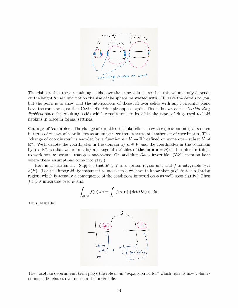
The claim is that these remaining solids have the same volume, so that this volume only dependson the height h used and not on the size of the sphere we started with. I’ll leave the details to you,but the point is to show that the intersections of these left-over solids with any horizontal planehave the same area, so that Cavieleri’s Principle applies again. This is known as the Napkin RingProblem since the resulting solids which remain tend to look like the types of rings used to holdnapkins in place in formal settings.

Change of Variables. The change of variables formula tells us how to express an integral writtenin terms of one set of coordinates as an integral written in terms of another set of coordinates. This“change of coordinates” is encoded by a function φ : V → Rn defined on some open subset V ofRn. We’ll denote the coordinates in the domain by u ∈ V and the coordinates in the codomainby x ∈ Rn, so that we are making a change of variables of the form u = φ(x). In order for thingsto work out, we assume that φ is one-to-one, C1, and that Dφ is invertible. (We’ll mention laterwhere these assumptions come into play.)

Here is the statement. Suppose that E ⊆ V is a Jordan region and that f is integrable overφ(E). (For this integrability statement to make sense we have to know that φ(E) is also a Jordanregion, which is actually a consequence of the conditions imposed on φ as we’ll soon clarify.) Thenf φ is integrable over E and:∫

φ(E)f(x) dx =

∫Ef(φ(u))| detDφ(u)| du.

Thus, visually:

The Jacobian determinant term plays the role of an “expansion factor” which tells us how volumeson one side relate to volumes on the other side.

74

Some of the assumptions can be relaxed a bit: we only need φ to be one-to-one on E away froma set of Jordan measure zero and similarly we only need Dφ to be invertible on E away from a set ofJordan measure zero. This makes sense, since what happens on these sets of Jordan measure zerocan’t possibly affect the integrals in question. The requirement that φ be one-to-one guaranteesthat φ(E) is only “traced out once”, which we’ll clarify in the following example.

Example. Let us run through the standard conversion you would have seen in a multivariablecalculus course from rectangular to polar coordinates in double integrals, in order to make sure thatthe various assumptions in the change of variables formula indeed hold in this case. The functionφ : R2 → R2 in this case is defined by φ(r, θ) = (r cos θ, r sin θ). This is C1 and has Jacobiandeterminant given by:

detDφ(r, φ) = det

(∂φ1∂r

∂φ1∂θ

∂φ2∂r

∂φ2∂θ

)= det

(cos θ −r sin θsin θ r cos θ

)= r.

Thus this Jacobian matrix is invertible as long as r 6= 0, so this fails to be invertible only at theorigin which is okay since (0, 0) has Jordan measure zero.

Take E = [0, 1] × [0, 2π], which is a Jordan region. Then φ(E) = B1(0, 0), the closed unitdisk of radius 1. Note that this is also a Jordan region, which as mentioned before is actually aconsequence of the assumptions we have on φ. Note that φ is not one-to-one on all of E since

φ(r, 0) = φ(r, 2π) for all r,

but that it only fails to be one-to-one along the bottom and top edges of the rectangle E, whichhave Jordan measure zero; as mentioned before, this is good enough for the change of variablesformula to be applicable. Thus for some integrable function f : φ(E)→ R, the changes of variablesformula gives: ∫

closed unit diskf(x, y) d(x, y) =

∫[0,1]×[0,2π]

f(r cos θ, r sin θ) r d(r, θ),

just as you would expect.Suppose that instead we took E = [0, 1]× [0, 4π], which still has image φ(E) equal to the closed

unit disk. For the constant function f = 1, if the changes of variables formula we’re applicable wewould get: ∫

closed unit diskd(x, y) =

∫[0,1]×[0,4π]

r d(r, θ) =

∫ 4π

0

∫ 1

0r dr dθ = 2π,

which is nonsense because we know that the left hand side should equal the area of the unit disk,which is π. (Note the use of Fubini’s Theorem when computing the integral in polar coordinatesas an iterated integral.) The problem is now that φ fails to be one-to-one throughout E since

φ(r, θ) = φ(r, θ + 2π) for all r and 0 ≤ θ ≤ 2π,

and so the region on which φ is not one-to-one no longer has Jordan measure zero. Thus the changeof variables formula is not applicable in this case. Geometrically, the problem is that allowing θto go all the way up to 4π gives two copies of the unit disk superimposed on one another, whichmeans that the unit disk is “traced out twice”.

Outline of proof of change of variables formula. The proof of the change of variables formulais quite involved, requiring multiple steps. The book divides these into various lemmas, and youcan see that it takes multiple pages to work it all out. Here we only give an outline, emphasizingwhere the various assumptions we make come into play. Here are the basic steps required:

75

• Step 0: show that if φ is C1, one-to-one, and has invertible Jacobian matrix, then it sendsJordan regions to Jordan regions. I’m calling this Step 0 because it is actually done inSection 12.1 in the book as Theorem 12.10, so way before the change of variables section.This guarantees that the regions of integration in both integrals showing up in the changeof variables formula are indeed Jordan regions. As mentioned previously, the one-to-one andinvertibility requirements can be relaxed a bit.

• Step 1: show that the change of variables formula holds in the special case where E is arectangle and f is the constant function 1. This is Lemma 12.44 in the book, which we’ll givesome geometric intuition for in a bit.

• Step 2: show that the change of variables formula holds for various pieces of the Jordan regionE and an arbitrary integrable function f . This is Lemma 12.43 in the book, and all stepsso far are summarized as Lemma 12.45. This is also the step where it is shown that f φ isautomatically integrable as a consequence of our assumptions. The “various” pieces alludedto above come from the open sets on which φ is locally invertible as a consequence of theInverse Function Theorem.

• Step 3: use compactness to show that what happens over the “local” pieces of E gives therequire formula over all of E. This is Theorem 12.46 in the book. From the previous stepsyou end up covering E with various open rectangles, and compactness of E allows us to workwith only finitely many of these.

As mentioned, the details are are quite involved, but since Jordan regions can in a sense beapproximated by rectangles (an idea which is used in Step 2), the truly key part is Step 1. Thisis also the step which explains where the Jacobian determinant factor in the formula comes from,which has a linear algebraic origin. (Don’t forget that locally, calculus is just linear algebra afterall!) We finish with the geometric intuition behind Step 1.

Geometric intuition behind change of variables. Suppose that E is a rectangle and that weare given some grid on it. Then φ transforms this into a possibly “curved grid” on φ(E):

Since φ is differentiable, the Jacobian matrix Dφ provides a good approximation to the behavior off , and Dφ roughly transforms a small rectangle in the grid on E into a small “curved parallelogram”in the “grid” on φ(E). According to the geometric interpretation of determinants from linearalgebra, the volume of the this parallelogram is related to the area of the rectangle from which itcame by:

area of φ(R) = | detDφ(p)|(area of R).

76

Thus given an outer sum∑

i |Ri| for E, we get a corresponding “outer sum” for φ(E) of the form:∑i

|φ(Ri)| =∑i

|detDφ(pi)||Ri|.

Note that this is not quite an outer sum since we don’t have an honest grid on φ(E), but rathera curved grid. Also note that since φ is C1, so that Dφ is continuous, we have some control overhow changing the grid on E will alter the grid on φ(E).

Now, since φ is C1 with invertible Jacobian, the Inverse Function Theorem implies that φ−1

is also C1. The Jacobian matrix Dφ−1 transforms the curved grid on φ(E) into the original gridon E. Since Dφ−1 is continuous, given an honest grid on φ(E) which approximates the curvedgrid, the curved grid on E resulting from this honest grid after applying Dφ−1 will approximatethe original grid on E fairly well. (A mouthful!) Using these ideas we can relate outer, lower, andupper sums on one side to those on the other side, and after some magic we get Step 1.

Important. For a one-to-one, C1 change of variables x = φ(u) with invertible Jacobian matrix,we have ∫

φ(E)f(x) dx =

∫Ef(φ(u))|detDφ(u)| du

whenever everything involved in this formula makes sense, meaning that E should be a Jordanregion and f should be integrable on φ(E). A key takeaway is that the Jacobian determinantdetDφ tells us how volumes are transformed under a change of variables.

May 11, 2015: Curves

Today we started working towards our final topic: the theorems of vector calculus. As a firststep we defined and looked at various properties of curves, most of which should be familiar froma previous multivariable calculus course. A key takeaway is that most things we do with curvesare done with respect to specific parametric equations, but in the end the results we develop areindependent of the choice of parametric equations.

Warm-Up 1. We compute the value of the integral∫∫E

cos(3x2 + y2) d(x, y)

where E is the elliptical region defined by x2 + y2/3 ≤ 1. Note that this integral exists since theintegrand is continuous.

We use the change of variables x = r cos θ, y =√

3r sin θ, which we can describe using thefunction φ : [0, 1]× [0, 2π]→ R2 defined by

φ(r, θ) = (r cos θ,√

3r sin θ).

This is C1, one-to-one away from a set of volume zero, and has Jacobian determinant

detDφ = det

(cos θ −r sin θ√3 sin θ

√3r cos θ

)=√

3r,

which is nonzero away from a set of volume zero as well. Since E = φ([0, 1]× [0, 2π]) and 3x2 +y2 =3r2, the change of variables formula applies to give:∫∫

Ecos(3x2 + y2) d(x, y) =

∫∫[0,1]×[0,2π]

cos(3r2)|√

3r| d(r, θ).

77

By Fubini’s Theorem, we have:∫∫[0,1]×[0,2π]

cos(3r2)|√

3r| d(r, θ) =

∫ 2π

0

∫ 1

0

√3r cos(3r2) dr dθ =

∫ 2π

0

√3

6sin 3 dθ =

π sin 3√3,

and thus∫∫E cos(3x2 + y2) d(x, y) = π sin 3/

√3 as well.

Warm-Up 2. Suppose that f : Rn → Rn is C1, one-to-one, and has invertible Jacobian matrix atevery point. We show that for each x0 ∈ Rn,

limr→0+

Vol(f(Br(x0)))

Vol(Br(x0))= | detDf(x0)|.

(This is almost the same as Exercise 12.4.6 on the homework, only there we do not assume that fis one-to-one. I’ll leave it to you to think about how to get around this subtlety.)

First, we can rewrite the numerator of the fraction of which we are taking the limit as:

Vol(f(Br(x0))) =

∫f(Br(x0))

dx =

∫Br(x0)

|detDf(u)| du

where we use x = f(u) as a change of variables, which we can do given the assumptions on f . Thusthe fraction of which we are taking the limit is

Vol(f(Br(x0)))

Vol(Br(x0))=

1

Vol(Br(x0))

∫Br(x0)

|detDf(u)| du.

Since f is C1, the map u 7→ Df(u) is continuous, and hence so is u 7→ |detDf(u)| since theoperation of taking the determinant of a matrix is a continuous one given that determinants canbe expressed as polynomials in the entries of a matrix. Thus the integrand in the resulting integralis continuous at x0, so Exercise 12.2.3 from the previous homework gives

limr→0+

Vol(f(Br(x0)))

Vol(Br(x0))= lim

r→0+

1

Vol(Br(x0))

∫Br(x0)

| detDf(u)| du = |detDf(x0)|

as claimed.

Calculus is linear algebra, redux. The previous result should be viewed as another instance ofthe fact that, locally, multivariable calculus is just linear algebra. Indeed, the linear algebraic factwe are generalizing here is that for an invertible matrix A:

Vol(A(Ω))

Vol(Ω)= | detA|

for any Jordan region Ω with nonzero volume. The result above says that is true “in the limit” fora more general C1 function with invertible Jacobian. Rewriting this equality as

Vol(A(Ω)) = |detA|Vol(Ω)

suggests that the entire change of variables formula itself should be viewed as the non-linear analogof this linear algebraic fact, which we alluded to when outlining the proof of the change of variablesformula.

78

Curves. A “curve” in Rn should be what we expect it to be, namely some sort of 1-dimensionalobject. To give a precise definition, we say that a Cp curve in Rn is the image C of a Cp functionφ : I → Rn where I is an interval and φ is one-to-one in the interior Io. To be clear, the curve Cbeing described is the one in Rn with parametric equations given by

φ(t) = (x1(t), . . . , xn(t)), t ∈ I

where (x1, . . . , xn) are the component of φ. We call φ : I → Rn a parametrization of C. Forthe most part, C1 curves—i.e. curves which can be described using continuously differentiableparametric equations—are what we will be interested in.

We say that a curve with parametrization φ : I → Rn is an arc is I is a closed interval [a, b] (soarcs have a start point and an end point), is closed if it is an arc and φ(a) = φ(b), and is simple if itdoes not intersect itself apart from possibly the common start and end point in the case of a closedcurve. Simple, closed curves in R2 are the ones which divide the plane into two pieces: a piece“interior” to the curve and a piece “exterior” to it. Look up the famous Jordan Curve Theorem tolearn more about this.

Smooth Curves. A curve C ⊆ Rn is said to be smooth at a point x0 if there exists a C1

parametrization φ : I → Rn of C such that φ′(t0) 6= 0 where t0 is the point in I which givesφ(t0) = x0. A curve is smooth if it is smooth at each of its points.

As we will show in a bit, the point is that smooth curves are the ones which have well-definedtangent lines. To clarify one possible subtlety in the definition, to say that a curves is smooth at apoint means that φ′(t0) 6= 0 for some parametrization, but it is not true that every parametrizationof a smooth curve has this property. For instance, the unit circle has parametric equations

φ(t) = (cos t, sin t) for t ∈ [0, 2π],

and since φ′(t) = (− sin t, cos t) is never 0, the unit circle is smooth everywhere. However, we canalso take

ψ(t) = (cos t3, sin t3) for t ∈ [0,3√

2π]

as parametric equations for the unit circle, but in this case

ψ′(t) = (−3t2 sin t3, 3t2 cos t3)

is 0 at t = 0, so this would be a non-smooth parametrization of the smooth unit circle. So, wecan rephrase the definition of smoothness as saying that a smooth curve is one which has a smoothparametrization, even though it may have non-smooth parametrizations as well.

Why we care about smooth curves. To justify the definition of smoothness given above,we show that smooth curves in R2 have well-defined tangent lines. (Later we will also see thatsmooth curves are the ones which have well-defined “directions”.) We assume that the only typesof curves we can precisely define tangent lines for are those which are graphs of single-variablefunctions (indeed, the whole point of the definition of differentiability for a single-variable functionis to capture the idea that the graph should have a well-defined tangent line), so the point is toshow that a smooth curve in R2 can, at least locally, be described by such graphs. This will anapplication of the Implicit Function Theorem.

So, suppose that C ⊆ R2 is a smooth C1 curve with smooth C1 parametrization φ : I → R2.Pick a point x0 ∈ C and t0 ∈ I such that φ(t0) = x0. Then we have parametric equations

x = φ1(t) y = φ2(t)

79

where (φ1, φ2) are the components of φ. Since φ is a smooth parametrization,

φ′(t0) = (φ′1(t0), φ′2(t0)) 6= (0, 0),

so at least one component is nonzero—say that φ′1(t0) 6= 0. By the Implicit Function Theorem, wecan then solve for y in terms of x locally near x0 in the given parametric equations, or to work itout a little more explicitly, by the Inverse Function Theorem we can solve for t in terms of x in

x = φ1(t)

locally near x0 to get t = φ−1(x) where φ−11 is C1, and then plugging into the second parametric

equation givesy = (φ2 φ−1

1 )(x)

which expresses y as a C1 function of x, at least near x0. Thus near x0, the curve C is the graphof the function f = φ2 φ−1

1 , so the curve has a well-defined tangent line at x0 = (x0, y0) given by

y = f(x0) + f ′(x0)(x− x0).

Important. A smooth curve is one which has a smooth parametrization. Geometrically, thisis precisely the condition needed to guarantee that the curve has well-defined tangent lines andtangent vectors.

Arclength. Now we can define the notion of the arclength of a smooth C1 arc. Suppose thatC ⊆ Rn is a smooth C1 arc with smooth C1 parametrization φ : [a, b] → Rn. The arclength of Cis by the definition the value of ∫ b

a

∥∥φ′(t)∥∥ dtwhere ‖·‖ denotes the usual Euclidean norm. (This is likely a definition you saw in a previouscourse.) The intuition is that φ′(t) gives a vector tangent to the curve at a given point, so ‖φ′(t)‖gives the length of a little infinitesimal piece of C and this integral is then adding up these infinites-imal lengths to get the total length.

Arclength is independent of parametrization. In order for this to be a good definition,we have to know that the number obtained solely depends on the curve C itself and not on theparametrization used. So, suppose that ψ : [c, d] → Rn is another smooth parametrization of C.We take it as a given that for any two such parametrizations ψ : [c, d]→ Rn and φ : [a, b]→ Rn canbe related by a “change of variables” function τ : [c, d]→ [a, b] such that ψ = φ τ , which describeshow to move from the parameter u in ψ to the parameter t = τ(u) in φ:

80

That such a τ exists is given as Remark 13.7 in the book, which you should check on your own.With this τ at hand, we have first using a change of variables:∫

[a,b]|φ′(t)| dt =

∫τ([c,d])

|φ′(t)| dt =

∫[c,d]|φ′(τ(u))||τ ′(u)| du.

Since ψ = φ τ , the chain rules gives ψ′(u) = φ′(τ(u))τ ′(u), so this final integral is∫[c,d]|φ′(τ(u))||τ ′(u)| du =

∫[c,d]|ψ′(u)| du,

so ∫ b

a|φ′(t)| dt =

∫ d

c|ψ′(u)| du

as required in order to say that φ and ψ give the same arclength.

Line integrals. Given a smooth C1 arc C in Rn with parametrization φ : [a, b] → Rn and acontinuous function f : C → R, we define the line integral of f over C to be:∫

Cf ds =

∫ b

af(φ(t))

∥∥φ′(t)∥∥ dt.This integral essentially “adds up” the values of f along the curve C, and the fact that φ is C1 andthat f is continuous guarantees that this integral exists. In a previous course you might have seenthis referred to as a scalar line integral, to distinguish it from so-called vector line integrals whicharise when integrating vector fields along curves—we’ll look at this type of line integral later on.

Even though the definition given depends on a parametrization of C, an argument similar tothat for arclength shows that the line integral of f over C is independent of the parametrizationused. In fact, we can also try to define the integral

∫C f ds via an upper/lower sum approach which

makes no reference to parametrizations at all; we’ll outline how to do this later on and argue thatthis approach gives the same value for

∫C f ds as to how we’ve defined it here.

Important. The line integral of a continuous function f : C → R over a smooth C1 arc C isindependent of parametrization. In the case where f is the constant function 1, this line integralgives the arclength of C.

May 13, 2015: Surfaces

Today we spoke about surfaces, where as we did last time with curves, the point is to give precisedefinitions and justifications for concepts you would have seen in a previous multivariable calculuscourse. Note that everything we now do is an analog of something we did for curves.

Another approach to arclength. Before moving on to surfaces, we give another reason as towhy the definition we gave for arclength last time makes sense geometrically, by relating it toanother possible definition. This is all covered in the optional material at the end of Section 13.1in the book.

The idea is that to define the length of a curve we can also argue using “line segment approxi-mations”. Say we are given some curve, and choose a finite number of points along it:

81

The distances d(pi, pi−1) (where d denotes the Euclidean distance) between successive points givesome sort of approximation to the length of the curve between those points, and the total sum:∑

i

d(pi, pi−1)

then underestimates the actual length of the curve. Taking more and more points results in betterand better approximations, so we can try to define the length as the supremum of such sums:

arclength of C = sup

∑i

d(pi, pi−1)

.

Curves for which this quantity is finite are called rectifiable, and the claim is that for rectifiablesmooth C1 curves, this definition of arclength agrees with the previous one.

The idea behind the proof is as follows. Choose a parametrization φ : [a, b] → Rn of C and apartition of [a, b]. Then the points φ(x0), φ(x1), . . . , φ(xn) give successive points on the curve, andthe distance between then are given by the expressions

‖φ(xi)− φ(xi−1)‖ .

Thus the sum over the entire partition is∑i

‖φ(xi)− φ(xi−1)‖ .

Now, using some version of the Mean Value Theorem, we can approximate these terms by

‖φ(xi)− φ(xi−1)‖ ≈∥∥φ′(xi)∥∥∆xi,

so ∑i

‖φ(xi)− φ(xi−1)‖ ≈∑i

∥∥φ′(xi)∥∥∆xi.

But the right-hand side can now be viewed as a Riemann sum for the integral∫ ba ‖φ

′(t)‖ dt, sotaking supremums of both sides gives the result. This is only meant to be a rough idea, but youcan check the book for full details.

One final thing to note: this approach to defining arclength only depends on the Euclideandistance d, and so can in fact be generalized to arbitrary metric spaces. The result is a definitionof arclength which makes sense in any metric space!

82

Warm-Up. Suppose that f : I → R is a C1 function on some interval I ⊆ R such that

|f(θ)|2 + |f ′(θ)|2 6= 0 for all θ ∈ I.

We show that the curve defined by the polar equation r = f(θ) is a smooth C1 curve.The curve we are looking at is the one consisting of all points in R2 whose polar coordinates

satisfy r = f(θ). Thus our curve is given parametrically by:

x = r cos θ = f(θ) cos θ y = r sin θ = f(θ) sin θ.

Since f is C1, the function φ : I → R2 given by φ(θ) = (f(θ) cos θ, f(θ) sin θ) is C1 as well so we dohave a C1 curve. To check smoothness we compute:

x′(θ) = f ′(θ) cos θ − f(θ) sin θ y′(θ) = f ′(θ) sin θ + f(θ) cos θ.

Then ∥∥(x′(θ), y′(θ))∥∥ =

√(f ′(θ) cos θ − f(θ) sin θ)2 + (f ′(θ) sin θ + f(θ) cos θ)2

=√f ′(θ)2 + f(θ)2 6= 0

after simplification. Thus φ′(θ) = (x′(θ), y′(θ)) is nonzero everywhere, so C is smooth as claimed.

Surfaces. Intuitively, a surface should be a “2-dimensional” object in R3. To make this precise, wesay that a Cp surface in R3 is the image S of a Cp function φ : E → R3 defined on a closed Jordanregion E in R2 which is one-to-one on Eo. As with curves, we call φ : E → R3 a parametrizationof S and its components (φ1, φ2, φ3) give us parametric equations

x = φ1(u, v), y = φ2(u, v), z = φ3(u, v) with (u, v) ∈ E

for S. The fact that there are two parameters in these equations is what makes S two-dimensional.We note that, as with curves, a given surface can be expressed using different sets of parametric

equations. In general, if φ : E → R3 and ψ : D → R3 are two parametrizations of a surface S, thereis a “change of variables” function τ : D → E such that ψ = φ τ , which tells us how to move fromparameters (s, t) for ψ to parameters (u, v) = τ(s, t) for φ:

The proof of this fact is similar to the proof of the corresponding fact for curves given in the book.

83

Example. Suppose that S is the portion of the cone z =√x2 + y2 for 0 ≤ z ≤ h, where h is some

fixed height. One set of parametric equations for S is

φ(u, v) = (u, v,√u2 + v2) with (u, v) ∈ Bh(0, 0).

Note however that this parametrization is not C1 since the z-component is not differentiable at(u, v) = (0, 0), which corresponds to the point (0, 0, 0) on the cone.

Instead, the parametrization given by

ψ(r, θ) = (r cos θ, r sin θ, r) with (r, θ) ∈ [0, h]× [0, 2π]

is C1. (In fact, this parametrization is C∞, showing that the cone is a C∞ surface.)

Smooth surfaces and normal vectors. Suppose that φ : E → R3 is a Cp (C1 will usually beenough) parametrization of a surface S. Denote the parameters by (u, v) ∈ E. Holding v fixed ata point and varying u results in a parametrization φ(·, v) of a curve on S, and thus differentiatingwith respect to u gives a vector tangent to the surface, which we denote by φu. Similarly, holdingu fixed gives a parametrization φ(u, ·) of another curve on S with tangent vector φv obtained bydifferentiating with respect to v.

We say that S is smooth at a point (x0, y0, z0) = φ(u0, v0) if the cross product

(φu × φv)(u0, v0)

is nonzero at that point, in which we case we call (φu×φv)(u0, v0) a normal vector to S at φ(u0, v0).(Recall that this cross product is perpendicular to both tangent vectors φu and φv, which intuitivelysuggests that it should indeed be perpendicular to the surface S.) We say that S is smooth if itis smooth everywhere. This smoothness condition is what guarantees that well-defined tangentplanes exist, as we will see in the Warm-Up next time. For now we mention that, as we saw withcurves, a smooth surface may have non-smooth parametrizations—all that matters is that a smoothparametrization exists.

Concretely, if φ = (φ1, φ2, φ3) are the components of φ, then:

φu × φv =

∣∣∣∣∣∣i j k∂φ1∂u

∂φ2∂u

∂φ3∂u

∂φ1∂v

∂φ2∂v

∂φ3∂v

∣∣∣∣∣∣ =

(∂φ2

∂u

∂φ3

∂v− ∂φ2

∂v

∂φ3

∂u,−∂φ1

∂u

∂φ3

∂v+∂φ1

∂v

∂φ3

∂u,∂φ1

∂u

∂φ2

∂v− ∂φ1

∂v

∂φ2

∂u

).

But note that the first component here can be viewed as the Jacobian determiant of the matrix:

D(φ2, φ3) :=

(∂φ2∂u

∂φ3∂u

∂φ2∂v

∂φ3∂v

),

and similarly the other components can also be viewed as Jacobian determinants. (Technically,the matrix above is the transpose of the Jacobian matrix D(φ2, φ3) of the function defined by thecomponents (φ2, φ3), but since a matrix and its transpose have the determinant this will not affectour formulas.) That is, we have:

φu × φv = (detD(φ2, φ3),−detD(φ1, φ3), detD(φ1, φ2))

where D(φi, φj) denotes the Jacobian matrix of the function defined by the components φi and φj .To save space, we will also denote this normal vector by Nφ.

84

Important. A surface is smooth if it has nonzero normal vectors at every point. (Often times, be-ing smooth except on a set of volume zero will be enough.) Geometrically, this condition guaranteesthe existence of a well-defined tangent plane.

Back to cone example. Consider the C1 parametrization ψ(r, θ) = (r cos θ, r sin θ, r) of the conez =

√x2 + y2 we saw earlier. We have:

ψr = (cos θ, sin θ, 1) and ψθ = (−r sin θ, r cos θ, 0),

so normal vectors are given by

ψr × ψθ = (−r sin θ,−r cos θ, r).

This is nonzero as long as r 6= 0, so we see that the cone is smooth everywhere except at (0, 0, 0),which is the “tip” of the cone. Note that it makes sense geometrically that the cone should not besmooth a this point, since the cone does not have a well-defined tangent plane at this point.

How normal vectors change under a change of variables. Suppose that φ : E → R3 andψ : D → R3 are two parametrizations of a smooth C1 surface S, with parameters (u, v) ∈ E and(s, t) ∈ D. We can directly relate the normal vectors obtained by φ to those obtained by ψ asfollows.

Recall that given these parametrizations there exists a C1 function τ : D → E such thatψ = φ τ . Also recall the expression derived previously for normal vectors determined by ψ:

ψs × ψt = (detD(ψ2, ψ3),−detD(ψ1, ψ3), detD(ψ1, ψ2)) .

Since ψ = φ τ , we also have

(ψi, ψj) = (φi, φj) τ, so detD(ψi, ψj) = (detD(φi, φj))(detDτ)

by the chain rule. Thus

ψs × ψt = (detDτ) (detD(φ2, φ3),−detD(φ1, φ3),detD(φ1, φ2)) ,

so we get thatNψ(s, t) = (detDτ(s, t))Nφ(τ(s, t)).

Hence normal vectors determined by ψ are obtained by multiplying those which are determined byφ by detDτ , so we should think of detDτ as a type of “expansion factor” telling us how normalvectors are affected under a change of variables. This is analogous to the formula

ψ′(u) = τ ′(u)φ′(τ(u))

relating tangent vectors determined by two parametrizations of a curve, where τ (a single-variablechange of coordinates in this case) plays a similar “expansion factor” role.

Surface area. Suppose that S is a smooth C1 surface. Given a smooth C1 parametrizationφ : E → R3 with parameters (u, v) ∈ E, we define the surface area of S to be:∫∫

E‖Nφ(u, v)‖ d(u, v).

85

Intuitively, ‖φu × φv‖ gives the area of the little infinitesimal portion of S swept out by the tangentvectors φu and φv, so to obtain the total surface area we add up all of these infinitesimal areas.

As with arclength, this definition is independent of parametrization, as we now show. Letψ : D → R3 be another smooth C1 parametrization with τ : D → E satisfying ψ = φ τ , so that(u, v) = τ(s, t). Then:∫∫

E‖Nφ(u, v)‖ d(u, v) =

∫∫τ(D)‖Nφ(u, v)‖ d(u, v)

=

∫∫D‖Nφ(τ(s, t))‖ |detDτ(s, t)| d(s, t)

=

∫∫D‖Nψ(s, t)‖ d(s, t)

where in the second line we’ve used a change of variables and in the final line the relation betweenNψ and Nφ derived above. Thus the surface area as computed using ψ is the same as that computedusing φ, so the surface area is independent of parametrization.

Surface integrals. Given a smooth C1 surface S with parameterization φ : E → R3 and acontinuous function f : S → R3, we define the surface integral of f over S to be:∫∫

Sf dS :=

∫∫Ef(φ(u, v)) ‖φu × φv‖ d(u, v),

which we interpret as adding up all the values of f as we vary throughout S. Note that the bookuses dσ instead of dS in the notation for surface integrals, but I like dS since it emphasizes betterthat we are integrating over a surface.

Using an argument similar to the one for surface area, it can be shown that this definition isalso independent of parametrization. As such, it makes sense to ask whether we can define surfaceintegrals without using parametrizations at all. We’ll come back to this next time.

Important. Surface integrals arise when integrating functions over surfaces and are independentof the parametrization used. In the case where f is the constant function 1, the surface integralgives the surface area.

May 15, 2015: Orientations

Today we spoke about orientations of both curves and surfaces. The point is that an orientationwill give us a to turn vector-valued functions (i.e. vector fields) into scalar-valued functions whichare then suitable for integration. Although curves are always orientable, we’ll see a well-knownexample of a surface which is not orientable.

Warm-Up. Suppose that S is a C1 surface which is smooth at (x0, y0, z0) ∈ S. We show that Sthen has a well-defined tangent plane at (x0, y0, z0). To be clear, we are assuming that the only typeof surface for which tangent planes are well-defined are graphs of differentiable functions f : V → Rwith V ⊆ R2(indeed, you can take the definition of differentiable in this setting as what it means forthe graph to have a well-defined tangent plane), so the claim is that locally near (x0, y0, z0) we canexpress S as the graph of such a function. This calls for the Implicit/Inverse Function Theorem.

Since S is smooth at (x0, y0, z0) there exists a parametrization φ : E → R3 with φ(u0, v0) =(x0, y0, z0) such that Nφ(u0, v0) 6= 0. Recall from last time the expression

Nφ(u0, v0) = (detD(φ2, φ3)(u0, v0),−detD(φ1, φ3)(u0, v0),detD(φ1, φ2)(u0, v0))

86

for the normal vector Nφ, where φ = (φ1, φ2, φ3) are the components of φ. Since this is nonzero, atleast one component is nonzero—we will assume that it is the third component which is nonzero.(This will result in expressing z as a function of x and y, so if instead one of the other componentswere nonzero we would end up expressing that corresponding variable as a function of the othertwo.) Our parametric equations looks like

x = φ1(u, v), y = φ2(u, v), z = φ3(u, v) (u, v) ∈ E,

so since detD(φ1, φ2)(u0, v0) 6= 0 and (φ1, φ2) is C1, the Inverse Function Theorem implies that wecan locally express u and v as a C1 function of x and y:

(u, v) = ψ(x, y) for some C1 function ψ

near (x0, y0, z0). This givesz = φ3(u, v) = (φ3 ψ)(x, y)

near (x0, y0, z0), which expresses S near this point as the graph of the C1 function f := φ3 ψ.Thus S has a well-defined tangent plane at (x0, y0, z0) which is explicitly given by

z = f(x0, y0) + fx(x0, y0)(x− x0) + fy(x0, y0)(y − y0)

where f is the C1 function defined above.

Line and surface integrals without parametrizations. Before moving on to orientations,we outline an attempt to define line and surface integrals without resorting to using parametricequations, mimicking the definitions we gave for integrals in terms of Riemann sums.

Suppose we are given some smooth C1 arc C ⊆ Rn and a continuous function f : C → Rn. Todefine the integral of f over C we can proceed by “partitioning” C by choosing successive pointsp0, p1, . . . , pn along C:

taking the infimum or supremum of f along the part of C between successive partition points, andthen forming “lower” and “upper” sums∑

i

(inf f)d(pi, pi−1) and∑I

(sup f)d(pi, pi−1)

where d denotes the ordinary Euclidean distance. (Note that we are essentially mimicking thealternate approach to defining arclength we outlined previously for “rectifiable” curves.) We wouldthen define

∫C f ds as the common value of the supremum of the lower sums or the infimum of the

87

upper sums. It turns out that this definition works perfectly well for rectifiable curves and givesthe value we would expect.

However, note now that, in this setting, we would expect a “change of variables” formula tohold just as it does for other types of integrals we’ve seen, where a change of variables functionφ : [a, b]→ Rn:

is precisely a parametrization of C! Thus, the change of variable formula in this setting would give∫Cf ds =

∫φ([a,b])

f ds =

∫[a,b]

f(φ(t))∥∥φ′(t)∥∥ dt,

where ‖φ′(t)‖ is the Jacobian expansion factor, which is precisely the definition we gave for∫C f ds

using a parametrization. Here’s the point: even if we defined line integrals using a Riemann sumapproach, the corresponding change of variables formula would imply that this definition to theone in terms of a parametrization, so rather than go through the trouble of defining such Riemannsums we simply take the parametrization approach as our definition, since in the end it would givethe correct answer anyway.

The same is true for surface integrals. We can define surface integrals independently of parametriza-tion by using certain upper and lower sums by picking “grids” on our surface, but in the end thechange of variables formula will say that the resulting integral is equal to the one given in termsof a parametrization, so we simply take the latter approach as our definition of a surface integral,thereby avoiding having to develop some extra theory. This is morally why constructions involvingcurves and surfaces always come down to some computations in terms of parametrizations: even ifwe could perform these constructions without using parametric equations, in the end we would getthe same types of objects using parametric equations anyway.

Orientations of curves. Given a smooth C1 curve C, an orientation on C is simply a choice ofcontinuously-varying unit tangent vectors along C. (We need the smoothness and C1 assumptionsto guarantee that our curves have well-defined tangent vectors, coming from the fact that they havewell-defined tangent lines.) Visually this just amounts to choosing a “direction” in which to followC. Concretely, if φ : I → Rn is a parametrization of C, then the unit tangent vectors

φ′(t)

‖φ′(t)‖

give us one possible orientation of C and the negative of these gives us the other possible orientation.To be clear, the C1 assumption says that the assignment t 7→ φ′(t) of a tangent vector to each

point on the curve is a continuous one, which is what we mean by saying that the tangent vectors

88

vary “continuously” along the curve. Note that because of this, for a connected curve we cannothave a scenario such as:

since some version of the Intermediate Value Theorem would imply that in this setting there mustbe some p = φ(t0) ∈ C at which φ′(t0) = 0, which is ruled out by the smoothness assumption onC. This is what guarantees that we are indeed choosing a single direction of movement along Cwhen we are picking an orientation.

When do parametrizations give the same orientation? We can easily determine when twoparametrizations φ, ψ of a curve C give the same orientation. Recall that we have ψ = φ τ forsome function t = τ(u). Then

ψ′(u) = φ′(τ(u))τ ′(u),

which implies that the unit vectors obtained from ψ and φ are the same precisely when τ ′(u) > 0.Thus two parametrizations give the same orientation when the “change of parameters” function τhas positive derivative everywhere.

For instance, consider the unit circle C in R2. This has possible parametric equations

φ(t) = (cos t, sin t) for 2π ≤ t ≤ 4π,

and alsoψ(u) = (cosu3, sinu3) for

3√

2π ≤ u ≤ 3√

4π.

In this case, τ(u) = u3 is the function satisfying ψ = φ τ , and since τ ′(u) = 3u2 is positive for all3√

2π ≤ u ≤ 3√

4π, we have that φ and ψ determine the same orientation on C, which makes sensesince both sets of parametric equations give the “counterclockwise” direction on the unit circle.

Orientations of surfaces. Given a smooth C1 surface S, an orientation on S is a choice ofcontinuously-varying unit normal vectors across S. (Again, the smoothness and C1 assumptionsguarantee that S has well-defined tangent planes, so the the notion of a “normal vector” makessense through S.) For a parametrization φ : E → R3 of S, the possible unit normal vectors aregiven by

φu × φv‖φu × φv‖

orφv × φu‖φu × φv‖

,

which are negatives of one another.The C1 assumption says that the map (u, v) 7→ φu×φv is continuous, which is what we mean by

“continuously-varying” normal vectors across S. The smoothness assumption guarantees that fora connected surface we can’t have one possible orientation along a portion of our surface but thenopposite orientation along another portion: for this to be true the Intermediate Value Theoremwould imply that at some point the normal vector would have to be zero, which is not allowed by

89

smoothness. However, there is a new subtlety with surfaces which we didn’t see for curves: not allsurfaces have well-defined orientations. We’ll come back to this in a it.

Recalling that the normal vectors of two parametrizations φ and ψ are related by

Nψ = (detDτ)Nφ

where τ is the change of parameters function satisfying ψ = φ τ , we see that two parametrizationsdetermine the same orientation when detDτ > 0 throughout S.

Example. Parametric equations for the unit sphere are given by:

X(φ, θ) = (sinφ cos θ, sinφ sin θ, cosφ) for (φ, θ) ∈ [0, π]× [0, 2π].

This gives the normal vectors

Xφ ×Xθ = sinφ(sinφ cos θ, sinφ sin θ, cosφ) = (sinφ)X(φ, θ).

Since sinφ > 0 for φ ∈ (0, π), this gives normal vectors which point in the same direction as thevector X(φ, θ) extending from the origin to a point on the sphere, so this gives the “outward”orientation on the sphere. The negatives of these normal vectors give the inward orientation. Notethat the possibility that certain normal vectors point outward and others inward is ruled out bythe Intermediate Value Theorem and the fact that X is a C1 parametrization, as mentioned earlier.

Non-orientable surfaces. Consider the surface S with C1 parametrization

φ(u, v) =((

1 + v sinu

2

)cosu,

(1 + v sin

u

2

)sinu, v cos

u

2

)for (u, v) ∈ [0, 2π]×

[−1

2,1

2

].

A lengthy computation shows that

φu × φv = sinu

2

(cosu+ 2v

(cos3 u

2− cos

u

2

))i +

1

2

(4 cos

u

2− 4 cos3 u

2+ v(1 + cosu− cos2 u)

)j

− cosu

2

(1 + v cos

u

2

)k,

and from this it is possible (although tedious) to show that S is smooth everywhere.Now, note from the normal vector derived above that:

Nφ(0, 0) = (0, 0,−1) and Nφ(2π, 0) = (0, 0, 1).

However, going back to the parametric equations, we see that

φ(0, 0) = (1, 0, 0) = φ(2π, 0),

so the values (u, v) = (0, 0) and (u, v) = (2π, 0) of our parameters both determine the same pointon S. This is bad: using (u, v) = (0, 0) gave a normal vector of (0, 0,−1) at this point whileusing (u, v) = (2π, 0) gave a normal vector of (0, 0, 1), which points in the opposite direction. Theconclusion is that the given parametrization does not give a unique well-defined normal vector at(1, 0, 0). We will show as a Warm-Up next time that no choice of parametrization of this surfaceS gives a well-defined normal vector at (1, 0, 0), so the problem here is really a fault of the surfaceand not any specific choice of parametrization.

The lack of being able to define a unique normal vector at each point of S says that it is notpossible to give S an orientation, so we say that S is non-orientable. The problem is that we

90

cannot make a consistent choice of “continuously-varying” normal vectors across S. We will avoidsuch surfaces in this class since the types of integrals we will soon consider depend on having anorientation. This surface in particular is known as the Mobius strip, and is what you get if youtake a strip of paper, twist one end, and then glue the ends together—there’s a picture in thebook. Two other famous non-orientable surfaces are the Klein bottle and the real projective plane,although these really aren’t “surfaces” according to our definition since they cannot be embeddedin R3—rather, they would be examples of non-orientable surfaces in R4.

Important. An orientation of a curve is a continuous choice of unit tangent vectors along thecurve, and an orientation of a surface is a continuous choice of unit normal vectors across thesurface. All curves have orientations, but not all surfaces do.

May 18, 2015: Vector Line/Surface Integrals

Today we started talking about vector line/surface integrals, which the book calls oriented line/surfaceintegrals. These are the integrals which arise when wanting to integrate a vector field over a curveor surface, and are the types of integrals which the “Big Theorems of Vector Calculus” deal with.We reviewed some properties and even computed a couple of explicit examples.

Warm-Up. We justify a claim we made last time about the Mobius strip S, that the lack of havinga well-defined normal vector at every point throughout the surface really is a characteristic of thesurface itself and not a fault of the specific parametrization we previously gave. To be precise,the claim is that if ψ : D → R3 is any parametrization of S, then ψ does not assign to the point(1, 0, 0) ∈ S a well-defined unique normal vector.

Let φ : D → R3 be the parametrization we gave for S last time. The key thing to recall is thatfor these equations we have

Nφ(0, 0) = −k but Nφ(2π, 0) = k

even though φ(0, 0) and φ(2π, 0) both give the same point (1, 0, 0) on S. If τ : D → E is the changeof parameters function satisfying ψ = φ τ , then

Nψ(s, t) = (detDτ(s, t))Nφ(τ(s, t)).

In particular, take (s0, t0) to be one set of values which give (1, 0, 0) and (s1, t1) to be another, sothat τ(s0, t0) = (0, 0) and τ(s1, t1) = (2π, 0). Then

Nψ(s0, t0) = (detDτ(s0, t0))Nφ(0, 0) = −(detDτ(s0, t0))k

andNψ(s1, t1) = (detDτ(s1, t1))Nφ(2π, 0) = (detDτ(s1, t1))k.

But detDτ is either always positive or always negative since otherwise the Intermediate Value The-orem would imply that it was zero somewhere, contradicting the smoothness of these parametriza-tions. Thus in either case, the two vectors above will never point in the same direction since oneis going to be a positive multiple of k and the other a negative multiple of k. Since (s0, t0) and(s1, t1) both give the point (1, 0, 0) on S, this shows that ψ does not assign a unique normal vectorto this point as claimed.

Vector line integrals. Suppose that C is a smooth C1 oriented arc in Rn and that F : C → Rnis a continuous function. (Such an F is said to be a continuous vector field along C, which we

91

normally visualize as a field of little vectors varying along C.) We define the vector line integral(or oriented line integral) of F over C as: ∫

CF ·T ds

where T denotes the unit tangent vector field along C determined by the given orientation. To beclear, the orientation determines T, which is then used to turn the Rn-valued function F into anR-valued function F ·T, which is then integrated over the curve using a scalar line integral. Thisprocedure is why we care about orientations! Given a parametrization φ : [a, b]→ Rn of C, we get:∫

CF ·T ds =

∫ b

aF(φ(t)) · φ′(t)

‖φ′(t)‖∥∥φ′(t)∥∥ dt,

which gives the familiar formula∫C

F ·T ds =

∫ b

aF(φ(t)) · φ′(t) dt

you would have seen in a multivariable calculus course. (Of course, the value is actually independentof the parametrization.)

Geometrically, this integral measures the extent to which you move “with” or “against” theflow of F as you move along the curve. To be concrete, the dot product F · T is positive whenF and T point in the same “general” direction—i.e. when the angle between them is less than90–and is negative when F and T point in “opposite” directions—i.e. when the angle betweenthem is greater than 90— and the line integral then “adds up” all of these individual dot productcontributions.

Example 1. Just in case it’s been a while since you’ve looked at these types of integrals, we’ll doan explicit computation. Let C be the piece of the parabola y = x2 oriented from (π/2, π2/4) to(5π/4, 25π2/16) and let F : C → R2 be

F(x, y) =

(−y sinx

x2,cosx

2x

).

We use φ : [π/2, 5π/4]→ R2 defined by φ(t) = (t, t2) as a parametrization of C. Then:∫C

(F ·T) ds =

∫ 5π/4

π/2F(φ(t)) · φ′(t) dt

=

∫ 5π/4

π/2

(− t

2 sin t

t2,cos t

2t

)· (1, 2t) dt

=

∫ 5π/4

π/2(− sin t+ cos t) dt

= −√

2− 1.

Vector surface integrals. Suppose S is a smooth C1 oriented surface in R3 and that F : S → R3

is a continuous vector field on S. We define the vector surface integral (or oriented surface integral)of F over S as ∫∫

SF · n dS

92

where n denotes the unit normal vector field across S determined by the given orientation. Anal-ogously to the line integral case, the point is that the orientation determines n, which is then usedto turn the vector-valued function F into a scalar-valued function F · n, which is then integratedover S using a scalar surface integral. Given a parametrization φ : E → R3 of S such that φu × φvgives the correct direction for normal vectors, we get∫∫

SF · n dS =

∫∫E

F(φ(u, v)) · (φu × φv)‖φu × φv‖

‖φu × φv‖ d(u, v),

which gives the familiar formula∫∫S

F · n dS =

∫∫E

F(φ(u, v)) · (φu × φv) d(u, v)

you would have seen in a multivariable calculus course. As with all of these types of integrals, thevalue is independent of parametrization.

Geometrically, this integral measures the extent to which F “flows” across S either “with” or“against” the orientation. Indeed, the dot product F · n is positive when F points in the samegeneral direction as n and is negative when it points “opposite” the direction of n, and the surfaceintegral then adds up these individual quantities.

Example 2. We compute the vector surface integral of F = (−4, 0,−x) over the portion S ofthe plane x + z = 5 which is enclosed by the cylinder x2 + y2 = 9, oriented with upward-pointingnormal vectors. Parametric equations for S are given by:

φ(r, θ) = (r cos θ, r sin θ, 5− r cos θ) for (r, θ) ∈ [0, 3]× [0, 2π].

This givesφr × φθ = (cos θ, sin θ,− cos θ)× (−r sin θ, r cos θ, r sin θ) = (r, 0, r),

which gives the correct orientation since these normal vectors point upwards due to the positivethird-component. Thus∫∫

SF · n dS =

∫∫[0,3]×[0,2π]

F(φ(r, θ)) · (φr × φθ) d(r, θ)

=

∫ 2π

0

∫ 3

0(−4, 0,−r cos θ) · (r, 0, r) dr dθ

=

∫ 2π

0

∫ 3

0(−4r − r2 cos θ) dr dθ

= −36π.

Important. Vector line and surface integrals are both defined by using orientations to turn vector-valued vector fields into scalar-valued functions (via taking dot products with tangent or normalvectors), and then integrating the resulting functions. In terms of parametric equations, we get theformulas we would have seen previously in a multivariable calculus course.

Fundamental Theorem of Line Integrals. We say that a continuous vector field F : E → Rndefined on some region E ⊆ Rn is conservative on E if there exists a C1 function f : E → R suchthat F = ∇f . We call such a function f a potential function for F.

93

The value obtained when integrating a conservative field over a curve is given by the followinganalog of the Fundamental Theorem of Calculus for Line Integrals: if f : E → R is C1 and C ⊆ Eis a smooth oriented C1 arc in E, then∫

C∇f ·T ds = f(end point of C)− f(initial point of C).

Indeed, suppose that φ : [a, b]→ Rn is a parametrization of C. then∫C∇f ·T ds =

∫ b

a∇f(φ(t)) · φ′(t) dt.

By the chain rule, the integrand in this integral is the derivative of the single-variable functionobtained as the composition f φ:

(f φ)′(t) = ∇f(φ(t)) · φ′(t),

So by the single-variable Fundamental Theorem of Calculus we have:∫ b

a∇f(φ(t)) · φ′(t) dt =

∫ b

a(f φ)′(t) dt = f(φ(b))− f(φ(a)),

which gives ∫C∇f ·T ds = f(end point of C)− f(initial point of C)

as claimed.In particular, two immediate consequences are the following facts:

• If C1, C2 are two smooth C1 arcs with the same initial point and the same end point, then∫C1∇f · T ds =

∫C2∇f · T ds. This property says that line integrals of conservative vector

fields are path-independent in the sense that the value does only depends on the endpoints ofpath but not on the specific path chosen to go between those points.

• If C is a smooth closed curve, then∫C ∇f ·T ds = 0.

We will see next time that a field which has either of these properties must in fact be conservative.

Important. Line integrals of conservative fields can be calculated by evaluating a potential func-tion at the end and start points of a curve, and subtracting. This implies that line integrals ofconservative fields are path-independent and that the line integral of a conservative field over aclosed curve is always zero.

May 22, 2015: Green’s Theorem

Today we stated and proved Green’s Theorem, which relates vector line integrals to double integrals.You no doubt saw applications of this in a previous course, and for us the point is understand whyit is true and, in particular, the role which the single-variable Fundamental Theorem of Calculusplays in its proof.

Warm-Up. Suppose that F : E → Rn is a continuous vector field on a region E ⊆ Rn. We showthat line integrals of F are path-independent in E if and only if F has the property that its line

94

integral over any closed oriented curve in E is zero. Last time we saw that conservative fields haveboth of these properties, so now we show that these two properties are equivalent to one anotherfor any field. (We’ll see in a bit that either of these properties in fact implies being conservative.)

Suppose that line integrals of F in E are path-independent and let C be a closed oriented curvein E. Pick two points A and B on C and denote by C1 the portion of C which goes from A toB along the given orientation, and C2 the portion which goes from B back to A along the givenorientation:

We use the notation C1 +C2 for the curve obtained by following C1 and then C2, so C1 +C2 = C.Now, denote by −C2 the curve C2 traversed with the opposite orientation, so going from A to B.Then C1 and −C2 both start at A and end at B, so by the path-independence assumption we have∫

C1

F ·T ds =

∫−C2

F ·T ds.

Changing the orientation of a curve changes the sign of the line integral, so∫−C2

F ·T ds = −∫C2

F ·T ds, and hence

∫C1

F ·T ds+

∫C2

F ·T ds = 0.

Thus ∫C

F ·T ds =

∫C1+C2

F · T ds =

∫C1

F ·T ds+

∫C2

F · ds = 0,

showing that the line integral of F over a closed curve is zero as claimed.Conversely suppose that the line integral of F over any closed curve in E is zero. Let C1 and C2

be two oriented curves in E which start at the same point A and end at the same point B. Thenthe curve C1 + (−C2) obtained by following C1 from A to B and then C2 in the reverse directionfrom B back to A is closed, so our assumption gives∫

C1+(−C2)F ·T ds = 0.

But ∫C1+(−C2)

F ·T ds =

∫C1

F ·T ds+

∫−C2

F ·T ds =

∫C1

F ·T ds−∫C2

F ·T ds,

so∫C1

F ·T ds =∫C2

F ·T ds, showing that line integrals of F in E are path-independent.

95

Path-independence implies conservative. We now show that conservative fields are the onlyones with the properties given in the Warm-Up, at least for fields on R2. To be precise, we show thatif F : R2 → R2 is a continuous vector field such that its line integrals in R2 are path-independent,then F must be conservative. The same holds for Rn instead of R2 using the same proof, only withmore components. This result also holds for domains other than Rn, although the proof we givebelow has to be modified. (We’ll point out where the modification comes in.)

Denote the components of F by F = (P,Q), which are each continuous. Fix (x0, y0) ∈ R2 anddefine the function f : R2 → R by

f(x, y) =

∫C(x,y)

F ·T ds

where C(x, y) is any smooth C1 path from (x0, y0) to (x, y). The path-independence property ofF assures that f is well-defined in that the specific curve C used to connect (x0, y0) to (x, y) isirrelevant. The motivation for this definition comes from the Fundamental Theorem of Calculus:if g : [a, b] → R is continuous, then the function G(x) =

∫ xa g(t) dt obtained by integrating g is

differentiable with derivative g.We claim that f is differentiable (in fact C1) and has gradient ∇f = F. First we compute the

partial derivative of f with respect to x. For this we choose as a path connecting (x0, y0) to (x, y)the one consisting of the vertical line segment L1 from (x0, y0) to (x0, y), and then the horizontalline segment L2 from (x0, y) to (x, y). We have

f(x, y) =

∫L1

F ·T ds+

∫L2

F ·T ds.

Parametrizing L1 with φ1(t) = (x0, t), y0 ≤ t ≤ y gives∫L1

(P,Q) ·T ds =

∫ y

y0

(P (x0, t), Q(x0, t)) · (0, 1) dt =

∫ y

y0

Q(x0, t) dt

and parametrizing L2 with φ2(t) = (t, y), x0 ≤ t ≤ x gives∫L2

(P,Q) ·T ds =

∫ x

x0

(P (t, y), Q(t, y)) · (1, 0) dt =

∫ x

x0

P (t, y) dt,

so

f(x, y) =

∫ y

y0

Q(x0, t) dt+

∫ x

x0

P (t, y) dt.

Differentiating with respect to x gives

fx(x, y) = 0 + P (x, y) = P (x, y),

where the first term is zero since the first integral is independent of x and the second term is P (x, y)by the Fundamental Theorem of Calculus. (Note the assumption that P is continuous is used hereto guarantee that the derivative of the second integral is indeed P (x, y).)

Now, to compute fy(x, y) we choose a path consisting of the line segment C1 from (x0, y0) to(x, y0) and the line segment C2 from (x, y0) to (x, y). Then after parametrizing these segments wecan derive that

f(x, y) =

∫C1

F ·T ds+

∫C2

F ·T ds =

∫ x

x0

P (t, y0) dt+

∫ y

y0

Q(x, t) dt.

96

Differentiating with respect to y gives 0 for the first integral and Q(x, y) for the second, so

fy(x, y) = Q(x, y), and hence ∇f = (fx, fy) = (P,Q) = F,

showing that F is indeed conservative on R2.

Important. For a vector field F : D → Rn which is C1 on an open, connected region D ⊆ Rn, theproperties that F is conservative on D, that F has path-independent line integrals in D, and thatthe line integral of F over any closed curve in D is zero are all equivalent to one another.

Remarks. As mentioned before, the same is true for vector fields on Rn with the path-independenceproperty: we just repeat the same argument as above when differentiating with respect to othervariables, using appropriately chosen paths consisting of various line segments.

Also, the argument we gave works for other domains, as long as the line segments used are alwaysguaranteed to be in those domains. This is true, for instance, for convex domains. More generally,a similar argument works for even more general domains—open connected ones in particular–butmodifications are required since the line segments used may no longer be entirely contained in suchdomains; the way around this is to take paths consisting of multiple short horizontal and verticalsegments, where we move from (x0, y0) a bit to the right, then a bit up, then a bit to the right,then a bit up, and so on until we reach (x, y). It can be shown that there is a way to do this whilealways remaining within the given domain. (Such a path is called a polygonal path, and it was aproblem earlier in the book—which was never assigned—to show that such paths always exist inopen connected regions.)

One last thing to note. Let us go back to the expression derived in the proof above whenwanting to compute fx(x, y):

f(x, y) =

∫ y

y0

Q(x0, t) dt+

∫ x

x0

P (t, y) dt.

When computing fy(x, y) we opted to use another path, but there is no reason why we couldn’ttry to differentiate this same expression with respect to y instead. The first term is differentiablewith respect to y by the Fundamental Theorem of Calculus, and to guarantee that the second termis differentiable with respect to y we assume that P is C1. Then the technique of “differentiationunder the integral sign” (given back at the beginning of Chapter 11 in the book) says that theoperations of differentiation and integration can be exchanged:

∂

∂y

∫ x

x0

P (t, y) dt =

∫ x

x0

∂P

∂y(t, y) dt,

so we get

fy(x, y) = Q(x0, y) +

∫ x

x0

Py(t, y) dt.

Since we know ∇f = F, it must be that this expression equals Q(x, y):

Q(x, y) = Q(x0, y) +

∫ x

x0

Py(t, y) dt.

This is indeed true(!), and is a reflection of the fact that Py = Qx for a conservative C1 vector field:Py = fxy = fyx = Qx by Clairaut’s Theorem, where f being C2 is equivalent to F = ∇f being C1.Similarly, differentiating the expression

f(x, y) =

∫ x

x0

P (t, y0) dt+

∫ y

y0

Q(x, t) dt

97

obtained when wanting to compute fy(x, y) with respect to x gives:

P (x, y) = P (x, y0) +

∫ y

y0

Qx(x, t) dt,

which is also a true equality and reflects Py = Qx as well.

Green’s Theorem. Green’s Theorem relates line integrals to double integrals, and is a specialcase of Stokes’ Theorem, which we’ll talk about next time. The statement is as follows. Supposethat D ⊆ R2 is a two-dimensional region whose boundary ∂D is a piecewise, smooth, simple C1

curve with positive orientation, and that F = (P,Q) : D → R2 is a C1 vector field on D. Then∫∂D

(P,Q) ·T ds =

∫∫D

(Qx − Py) dA.

The “positive” orientation on ∂D is the one where, if you were to walk along ∂D in that direction,the region D would be on your left side. (This a bit of a “hand-wavy” definition, but is good enoughfor most purposes. Giving a more precise definition of the positive orientation on the boundarywould require having a more precise definition of “orientation”, which is better left to a full-blowncourse in differential geometry.)

The proof of Green’s Theorem is in the book. There are two key ideas: first, prove Green’sTheorem in the special case where D is particular “nice”, namely the case where pieces of itsboundary can be described as graphs of single-variable functions, and second glue such “nice”regions together to get a more general D. The second step involves using the Implicit FunctionTheorem to say that smoothness of ∂D implies you can indeed describe portions of ∂D as single-variable graphs. The first step boils down to the observation that the types of expressions

P (x, g1(x))− P (x, g2(x)) and Q(f2(y), y)−Q(f1(y), y)

you end up with (after using parametric equations) can be written—due the continuity of P andQ—as integrals:

P (x, g1(x))− P (x, g2(x)) =

∫ g2(x)

g1(x)−Py(x, t) dt and Q(f2(y), y)−Q(f1(y), y) =

∫ f2(x)

f1(x)Qx(t, y) dt

as a consequence of the Fundamental Theorem of Calculus. This introduction of an additionalintegral is what turns the line integral on one side of Green’s Theorem into the double integral onthe other side, and is where the Qx − Py integrand comes from. Check the book for full details.I point this out now since the same idea is involved in the proof of Gauss’s Theorem, suggestingthat Green’s Theorem and Gauss’s Theorem are the “same” type of result, which is an idea we’llcome back to on the final day of class.

Important. Green’s Theorem converts line integrals into double integrals, and its proof boils downto an application of the single-variable Fundamental Theorem of Calculus.

May 27, 2015: Stokes’ Theorem

Today we spoke about Stokes’ Theorem, the next “Big Theorem of Vector Calculus”. Stokes’Theorem relates line integrals to surface integrals, and is a generalization of Green’s Theorem tocurved surfaces; its proof (at least the one we’ll outline) uses the two-dimensional Green’s Theoremat a key step.

98

Warm-Up 1. Suppose that F = (P,Q) : U → R2 is a C1 vector field on an open set U ⊆ R2. Weshow that for any p ∈ U :

(Qx − Py)(p) = limr→0+

1

πr2

∫∂Br(p)

F ·T ds

where ∂Br(p) is oriented counterclockwise for any r > 0. Note that U being open guarantees thatfor small enough r > 0, the circle ∂Br(p) is contained in U , so that the line integral in questionmakes sense since F is defined along points of ∂Br(p).

The justifies the geometric interpretation of the quantity Qx − Py you might have seen in aprevious course: it measures the “circulation” of F around any given point, where counterclockwisecirculations are counted as positive and clockwise circulations are negative. Indeed, the line integral∫

∂Br(p)F ·T ds

measures the circulation of F around the circle of radius r around p, and so the limit—where wetake this circle getting smaller and smaller and closing in on p—is interpreted as the “circulation”around p itself. This is a special case of the geometric interpretation of the curl of a vector field,which we’ll come to after stating Stokes’ Theorem.

By Green’s Theorem, we have

1

πr2

∫∂Br(p)

F ·T ds =1

Vol(Br(p))

∫∫Br(p)

(Qx(x, y)− Py(x, y)) d(x, y).

Since F is C1, Qx − Py is continuous so a problem from a previous homework shows that

limr→0+

1

Vol(Br(p))

∫∫Br(p)

(Qx(x, y)− Py(x, y)) d(x, y) = (Qx − Py)(p),

which then gives the desired equality

(Qx − Py)(p) = limr→0+

1

Vol(Br(p))

∫∫Br(p)

(Qx(x, y)− Py(x, y)) d(x, y) = limr→0+

1

πr2

∫∂Br(p)

F ·T ds.

Warm-Up 2. Let F = (P,Q) be the vector field

F(x, y) =

(− y

x2 + y2,

x

x2 + y2

).

We show that F is conservative on the set R2 \ nonnegative x-axis obtained by removing theorigin and the positive x-axis from R2.

Let C be any simple smooth closed curve in R2 \ nonnegative x-axis and let D be the regionit encloses, so that C = ∂D. Then F is C1 on D and so Green’s Theorem gives∫

CF ·T ds = ±

∫∫D

(Qx − Py) dA

where the ± sign depends on the orientation of C. For this field we have

Qx =y2 − x2

x2 + y2= Py,

99

so Qx−Py = 0 and hence∫∫D(Qx−Py) dA = 0. Thus the line integral of F over any simple smooth

closed curve in R2 \nonnegative x-axis is zero, and so by an equivalence we established last time,this implies that F is conservative on R2 \ nonnegative x-axis.

Observation. Now, knowing that the field above F is conservative on R2 \ nonnegative x-axis,we can try to find a potential function for F over this region, which is a C2 function f : R2 \nonnegative x-axis → R satisfying ∇f = F. This is not something you’d be expected to able todo on the final, and I’m just mentioning this in order to illustrate an important property of thisspecific vector field.

To start with, a direct computation involving derivatives of the arctangent function will showthat:

∇(

tan−1 y

x

)= F.

However, f(x, y) = tan−1( yx

)is not defined for x = 0, so this does not give us a potential function

over all of R2\nonnegative x-axis yet. For now, we view this as defining our sought-after potentialonly in the first quadrant. The idea is now to extend this function to the second, third, and fourthquadrants in a way so that we have ∇f = F at each step along the way.

Another direction computation shows that the following is also true:

∇(− tan−1 x

y

)= F.

This is good since this new potential function is defined for x = 0, although it is no longer defined fory = 0. The point is that we will only try to use this expression to define the sought-after potentialover the second quadrant and on the positive y-axis, on which the potential we used above overthe first quadrant was not defined. However, we have to do this in a way which guarantees thepotential we’re defining (by piecing together local potentials) over the first and second quadrantsis in fact C1 even along the positive y-axis. For (x, y) in the first quadrant, y

x > 0 so as x→ 0 wehave y

x → +∞, and thus tan−1( yx) → π2 . The function − tan−1(xy ) has value 0 when x = 0, so the

function

− tan−1

(x

y

)+π

2

has value π2 on the positive y-axis. Thus the function defined by

tan−1(yx

)on the first quadrant and − tan−1

(x

y

)+π

2on the second quadrant

will indeed be C1 even on the positive y-axis. Since adding a constant to a function does not alterits gradient, this piece over the second quadrant still has gradient equal to F, so now we have a C1

function on the upper-half plane which has gradient F.We continue in this way, using the two arctangent expressions above to define the sought-after

potential over the remaining quadrants, where we add the necessary constants to ensure that westill get C1 functions along way as we “jump” from one quadrant to another:

100

For (x, y) in the second quadrant, xy < 0 so as y → 0 (i.e. as we approach the x-axis), we have

xy → −∞ and thus − tan−1

(xy

)+ π

2 → −(−π2 ) + π

2 = π. Thus defining the potential function over

the third quadrant and negative x-axis to be

tan−1(yx

)+ π

maintains the C1 condition and gradient equals F condition. For (x, y) in the third quadrant, yx > 0to as x→ 0 we get tan−1( yx) + π → 3π

2 , so we define our potential to be

− tan−1

(x

y

)+

3π

2

over the fourth quadrant and on the negative y-axis. The conclusion is that the function f :R2 \ nonnegative x-axis → R defined by:

f(x, y) =

tan−1

( yx

)x > 0, y > 0

− tan−1(xy

)+ π

2 x ≤ 0, y > 0

tan−1( yx

)+ π x < 0, y ≤ 0

− tan−1(xy

)+ 3π

2 x ≥ 0, y < 0

is C1 and satisfies ∇f = F, so f is a potential function for the conservative field F over the regionR2 \ nonnegative x-axis.

Now, note what happens if we take the same expression above, only we now consider it as afunction defined on R2 \ (0, 0, so including the positive x-axis. This seems plausible since theportion tan−1

( yx

)defining f over the first quadrant is in fact defined when y = 0, so we could

change the first case in the definition above to hold for x > 0, y ≥ 0, thereby giving a well-definedfunction on R2 \ (0, 0). However, if we take the limit of the portion of f defined in the thirdquadrant as (x, y) approaches the positive x-axis from below we would get a value of 2π, whichmeans that in order to preserve continuous the portion defined over the first quadrant would haveto be

tan−1(yx

)+ 2π

instead of simply tan−1( yx). Since we’re off by an additional 2π, this says that there is no way toextend the definition of f above to the positive x-axis so that it remains continuous, let alone C1,

101

which suggests that F =(− yx2+2 ,

xx2+y2

)should actually NOT be conservative over the punctured

plane R2 \ (0, 0). This is in fact true, as we can see from the fact that∫unit circle,

counterclockwise

F ·T ds = 2π

The fact that F is conservative over R2 \ nonnegative x-axis but not R2 \ (0, 0) is crucialin many applications of vector calculus, and in particular is related to the fact in complex analysisthat there is no version of the complex log function which is differentiable on the set of all nonzerocomplex numbers; if you want a differentiable log function in complex analysis, you must deletehalf of an axis or more generally a ray emanating from the origin in C. For this given field F, theline integral over any closed simple curve can only have one of three values:

∫C

(− y

x2 + y2,

x

x2 + y2

)·T ds =

2π if C encircles the origin counterclockwise

−2π if C encircles the origin clockwise

0 if C does not encircle the origin.

Manifold boundary. Before talking about Stokes’ Theorem, we must clarify a new use of theword “boundary” we will see. Given a surface S, we define its manifold boundary as follows. Givena point in S, if we zoom in on S near this point we will see one of two things: either S near thispoint will look like an entire disk, or S near this point will look like a half-disk:

The points near which S looks like a half-disk are called the manifold boundary points of S, andthe manifold boundary ∂S of S is the curve consisting of the manifold boundary points. Intuitively,the manifold boundary is the curve describing where there is an “opening” into S. A closed surfaceis one which has no manifold boundary; for instance, a sphere is a closed surface. Notationally, wedenote manifold boundaries using the same ∂ symbol as we had for topological boundaries, andwhich type of boundary we mean should be clear from context.

To distinguish this from our previous notion of boundary, we might refer to the previous notionas the topological boundary of a set. In general, the manifold and topological boundaries of a surfaceare quite different; they agree only for a surface fully contained in the xy-plane viewed as a subsetof R2. Similar notions of manifold boundary can be given for objects other than surfaces: the“manifold boundary” of a curve will be the set of its endpoints, and the “manifold boundary” of athree-dimensional solid in R3 is actually the same as its topological boundary.

An orientation on S induces a corresponding orientation on ∂S, which we call the positiveorientation on ∂S. The simplest way to describe this orientation is likely what you saw in aprevious course: if you stand on ∂S with your head pointing in the direction of the normal vector

102

determined by the orientation on S, the positive orientation on ∂S corresponds to the directionyou have to walk in in order to have S be on your “left” side. It is possible to give a more precisedefinition of this positive orientation, but this would require, as usual, a more precise definition oforientation in terms of linear algebra and differential geometry.

Stokes’ Theorem. Suppose that S is a piecewise smooth oriented C2 surface whose boundary ∂Sis a piecewise smooth C1 curve, oriented positively. Stokes’ Theorem says that if F = (P,Q,R) :S → R3 is a C1 vector field, then∫

∂SF ·T ds =

∫∫S

curl F · n dS

wherecurl F = (Ry −Qz, Pz −Rx, Qx − Py)

is the curl of F, which is a continuous vector field curl F : S → R3. Thus, Stokes’ Theorem relatesline integrals on one side to surface integrals of curls on the other.

We note that Green’s Theorem is the special case where S is a surface fully contained in thexy-plane. Indeed, here the normal vector n is k = (0, 0, 1) and

curl F · n = Qx − Py,

so the surface integral in Stokes’ Theorem becomes simply∫∫S(Qx−Py) dA as in Green’s Theorem.

One may ask: if Green’s Theorem is a consequence of Stokes’ Theorem, why prove Green’s Theoremfirst instead of simply proving Stokes’ Theorem and deriving Green’s Theorem from it? The answer,as we’ll see, is that the proof of Stokes’ Theorem uses Green’s Theorem in a crucial way.

Geometric meaning of curl. Suppose that F : R3 → R3 is a C1 vector field, so that curl F isdefined, and let n be a unit vector in R3. Fix p ∈ R3 and let Dr(p) be the disk of radius r centeredat p in the plane which is orthogonal to n at p. Then we have∫

∂Dr(p)F ·T ds =

∫∫Dr(p)

curl F · n dS

and

limr→0+

1

πr2

∫∫Dr(p)

curl F · n dS = curl F(p) · n

since the function q 7→ curl F(q) · n is continuous. Thus we get

curl F(p) · n = limr→0+

1

πr2

∫∂Dr(p)

F ·T ds,

giving us the interpretation the curl F(p) measures the “circulation” of F around the point p; inparticular, curl F(p)·n measures the amount of this circulation which occurs on the plane orthogonalto n. This is the geometric interpretation of curl you might have seen in a previous calculus course,and the point is that it follows from Stokes’ Theorem and the homework problem which tells ushow to compute the limit above.

Proof of Stokes’ Theorem. The proof of Stokes’ Theorem is in the book, and the basic strategyis as follows. As in the proof of Green’s Theorem, we look at a special case first and then piece

103

together these special surfaces to build up the general statement; the special case in this case isthat of a surface S given by the graph z = f(x, y) of a C2 function.

Let E be the portion of the xy-plane lying below S, and let (x(t), y(t)), t ∈ [a, b] be parametricequations for ∂E. Then

φ(t) = (x(t), y(t), f(x(t), y(t))), t ∈ [a, b]

are parametric equations for ∂S. Using this we can express the left-hand side of Stokes’ Theoremas ∫

∂SF ·T ds =

∫ b

aF(φ(t)) · φ′(t) dt.

After computing φ′(t) and writing out this dot product, the resulting expression can be written asanother dot product of the form:

(some two-dimensional field) · (x′(t), y′(t)),

which is the type expression you get in two-dimensional lines integrals. Indeed, this will write theline integral over ∂S as a line integral over ∂E instead:∫

∂SF ·T ds =

∫∂E

(some two-dimensional field) ·T ds.

To this we can now apply Green’s theorem, which will express this line integral over ∂E as adouble integral over E:∫

∂E(some two-dimensional field) ·T ds =

∫∫E

(some function) d(x, y).

Finally, the integrand in this double integral can be written as a dot product which looks like:

(Ry −Qz, Pz −Rx, Qx − Py) · (normal vector to S),

so that the double integral describes what you get when you use the parametrization

ψ(x, y) = (x, y, f(x, y)) (x, y) ∈ E

to compute the surface integral of curl F over S:∫∫E

(some function) d(x, y) =

∫∫S

curl F · n dS.

To recap, the process is: write the line integral of F over ∂S as a line integral over ∂E instead,apply Green’s Theorem to get a double integral over E, rewrite this double integral as the surfaceintegral of curl F over S.

Check the book for full details. The tricky thing is getting all the computations correct. Forinstance, in the first step you have to compute φ′(t) for

φ(t) = (x(t), y(t), f(x(t), y(t))),

where differentiating the third component z(t) = f(x(t), y(t)) here requires a chain rule:

z′(t) = fxx′(t) + fyy

′(t).

Thus(P,Q,R) · (x′(t), y′(t), fxx′(t) + fyy

′(t)) = (P + fx, Q+ fy) · (x′(t), y′(t)),

104

so that the “some two-dimensional field” referred to in the outline above is the field

(P +RRfx, Q+ fy).

This is the field to which Green’s Theorem is applied, in which we need to know:

∂

∂x(Q+Rfy)−

∂

∂y(P +Rfx).

Each of these derivatives again require chain rules since Q and R are dependent on x in two ways:

Q = Q(x, y, f(x, y)) R = R(x, y, f(x, y))

and P and R are dependent on y in two ways:

P = P (x, y, f(x, y)) R = R(x, y, f(x, y)).

We have:

∂

∂xQ(x, y, f(x, y)) = Qx +Qzfx and

∂

∂yP (x, y, f(x, y)) = Py + Pzfy,

and similar expressions for the derivatives of R. This all together gives the “some function” referredto in the outline above. Note that in this step there will be some simplifications in the resultingexpression using the fact that fyx = fxy since f is a C2 function.

We’ll stop here and leave everything else to the book, but notice how the curl of F naturally popsout of this derivation, in particular in the “some function” in the outline. Indeed, it was throughthis derivation that the curl was first discovered: historically, it’s not as if someone randomly wrotedown the expression

(Ry −Qz, Pz −Rx, Qx − Py)and then wondered what interesting properties this might have, but rather this expression showedup in the proof of Stokes’ Theorem and only after that was it identified as an object worth ofindependent study. The name “curl” historically came from the geometric interpretation in termsof circulation we gave earlier.

Important. Stokes’ Theorem relates the surface integral of the curl of a field over a surface tothe line integral of the “uncurled” field over the (manifold) boundary of that surface. The powerof Stokes’ Theorem in practice comes from relating one-dimensional objects (line integrals) to two-dimensional objects (surface integrals), and in giving geometric meaning to curl F.

May 29, 2015: Gauss’s Theorem

Today we spoke about Gauss’s Theorem, the last of the “Big Theorems of Vector Calculus”. Gauss’sTheorem relates surface integrals and triple integrals, and should be viewed in the same vein as theFundamental Theorem of Calculus, Green’s Theorem, and Stokes’ Theorem as a theorem whichtells us how an integral over the boundary of an object can be expressed as an integral over theentire object itself.

Warm-Up 1. We verify Stokes’ Theorem (i.e. compute both integrals in Stokes’ Theorem to seethat they are equal) for the vector field

F(x, y, z) = (2y − z, x+ y2 − z, 4y − 3x)

and the portion S of the sphere x2 + y2 + z2 = 4 where z ≤ 0, with outward orientation.

105

First we compute ∫∫S

curl F · n dS.

We havecurl F = (5, 2,−1) · n dS.

At a point (x, y, z) on S, the vector going from the origin to (x, y, z) itself is normal to S, son = 1

2(x, y, z) is a unit normal vector to the S at (x, y, z). Thus∫∫S

curl F · n dS =

∫∫S

1

2(5x+ 2y − z) dS.

The integral of 5x + 2y over S is zero due to symmetry (the integrand is odd with respect to avariable the surface is symmetric with respect to), so∫∫

Scurl F · n dS = −1

2

∫∫Sz dS.

Parametrizing S using

ψ(φ, θ) = (2 sinφ cos θ, 2 sinφ sin θ, 2 cosφ), (φ, θ) ∈ [π

2, π]× [0, 2π],

we have

ψφ × ψθ = (2 cosφ cos θ, 2 cosφ sin θ,−2 sinφ)× (−2 sinφ sin θ, 2 sinφ cos θ, 0)

= (4 sin2 φ cos θ, 4 sin2 φ sin θ, 4 sinφ cosφ),

so ‖ψφ × ψθ‖ = 4 sinφ. Hence

−1

2

∫∫Sz dS = −1

2

∫ 2π

0

∫ π

π/2(2 cosφ)(4 sinφ) dφ dθ = −1

2

∫ 2π

0−4 dθ = 4π

is the value of∫∫S curl F · n dS.

Now we compute∫∂S F · T ds. The (manifold) boundary of S is the circle of radius 2 in the

xy-plane with clockwise orientation. We parametrize ∂S using

φ(t) = (2 cos t,−2 sin t, 0), 0 ≤ t ≤ 2π,

we have∫∂S

F ·T ds =

∫ 2π

0F(φ(t)) · φ′(t) dt

106

=

∫ 2π

0(−4 sin t, 2 cos t+ 4 sin2 t, 8 sin t− 6 cos t) · (−2 sin t,−2 cos t, 0) dt

=

∫ 2π

0(8 sin2 t− 4 cos2 t− 8 sin2 cos t) dt

= 4π

after using sin2 t = 12(1− cos 2t) and cos2 t = 1

2(1 + cos 2t). Thus∫∂S F ·T ds =

∫∫S curl F · n dS as

claimed by Stokes’ Theorem.

Warm-Up 2. Suppose that G is a continuous vector field on R3. We say that surface integrals ofG are surface-independent if

∫∫S1

G ·n dS =∫∫S2

G ·n dS for any oriented smooth surfaces S1 andS2 with the same boundary and which induce the same orientation on their common boundary.We show that surface integrals of G are surface-independent if and only if the surface integral ofG over any closed surface is zero.

Before doing so, here’s why we care. First, this is the surface integral analog of the fact for lineintegrals we showed in a previous Warm-Up that line integrals of a field G are path-independent ifand only if the line integral of G over any closed curve is zero. Second, fields of the form G = curl Fwhere F is a C1 field always have these properties as a consequence of Stokes’ Theorem. Indeed,in the setup above, Stokes’ Theorem gives∫∫

S1

curl F · n dS =

∫∂S1=∂S2

F ·T ds =

∫∫S2

curl F · n, dS,

so surface integrals of curl F are surface-independent. Also, if S is closed, then ∂S = ∅ so∫∫S

curl F · n dS =

∫∂S

F ·T ds = 0

since the latter takes place over a region of volume zero, empty in fact. This is one of the manyreasons why curls play a similar role in surface integral theory that conservative fields do in lineintegral theory. (We’ll see a deeper reason why this analogy holds next time when we talk aboutdifferential forms.)

Suppose that surface integrals of G are surface-independent and let S be a closed orientedsurface. Slice through S to create two surfaces S1 and S2 with the same boundary, which is thecurve where the “slicing” occurred:

107

Note that the given orientations on S1 and S2 actually induce opposite orientations on their commonboundary. Thus S1 and −S2 induce the same orientation on their common boundary, so surface-independent gives ∫∫

S1

G · n dS =

∫∫−S2

G · n dS.

Since∫∫−S2

G · n dS = −∫∫S2

G · n dS, this in turned gives∫∫S=S1+S2

G · n dS =

∫∫S1

G · n dS +

∫∫S2

G · n dS = 0

as desired.Conversely suppose that the surface integral of G over any closed oriented surface is zero, and let

S1 and S2 be two oriented surfaces with the same boundary and which induce the same orientationon their common boundary. Glue S1 and −S2 along their common boundary to get a closed surfaceS. Since we switched the orientation on S2, this closed surface S = S1 ∪ (−S2) has a consistentorientation, and so is itself oriented. Our assumption gives∫∫

S1∪(−S2)G · n dS = 0,

so ∫∫S1

G · n dS −∫∫

S2

G · n dS = 0,

which in turns gives surface-independence.

Gauss’s Theorem. Suppose that E ⊆ R3 is a three-dimensional solid region whose boundary∂E is a piecewise smooth C1 surface, and let F = (P,Q,R) : E → R3 be a C1 vector field on E.Gauss’s Theorem (also called the Divergence Theorem) says that∫∫

∂EF · n dS =

∫∫∫E

div F dV

where div F = Px+Qy+Rz and where we give ∂S the outward orientation, meaning the orientationconsisting of normal vectors which point away from E. Thus, surface integrals over a closed surfacecan be expressed as triple integrals over the region enclosed by that surface.

Geometric meaning of divergence. Before talking about the proof of Gauss’s Theorem, wegive one application, which justifies the geometric meaning behind divergence you likely saw in aprevious course. The claim is that for a C1 field F on R3 and a point p ∈ R3,

div F(p) = limr→0+

1

Vol(Br(p))

∫∫∂Br(p)

F · n dS.

Here, ∂Br(p) is the sphere of radius r centered at p. The integral on the right measures the flowof F across this sphere, and so this equality says that div F(p) measures the “infinitesimal” flow ofF at p, where div F(p) > 0 means that there is a net flow “away” from p while div F(p) < 0 meansthere is a net flow “towards” p.

By Gauss’s Theorem we have∫∫∂Br(p)

F · n dS =

∫∫∫Br(p)

div F dV.

108

Thus

limr→0+

1

Vol(Br(p))

∫∫∂Br(p)

F · n dS = limr→0+

1

Vol(Br(p))

∫∫∫Br(p)

div F dV = div F(p)

since div F is a continuous function. This gives the required equality.

Proof of Gauss’s Theorem. The proof of Gauss’s Theorem is in the book, and follows the samestrategy as the proof of Green’s Theorem or Stokes’ Theorem: prove a special case where ∂E isgiven by the graphs of C1 functions, and then “glue” these special surfaces together.

Assuming that E is the region between the graphs of two C1 functions:

z = g2(x, y) and z = g2(x, y),

the boundary of E is then given by these two graphs. After setting up parametric equations foreach of these and using these to compute∫∫

∂S(0, 0, R) · n dS,

at some point we get an expression of the form

R(x, y, g2(x, y))−R(x, y, g1(x, y)),

which, due to the continuity of Rz, we can write as

R(x, y, g2(x, y))−R(x, y, g1(x, y)) =

∫ g2(x,y)

g1(x,y)Rz(x, y, t) dt

using the Fundamental Theorem of Calculus. This is the same type of thing we did in the proofof Green’s Theorem, and is the step which transforms the two-dimensional surface integral on oneside of Gauss’s Theorem to the three-dimensional triple integral on the other side. This is also thestep that explains where the Rz term in the divergence comes from. Doing the same for the field(P, 0, 0) gives the Px term and (0, Q, 0) gives the Qy term.

Check the book for full details, and next time we will see that these similarities in the proofs ofGauss’s and Green’s Theorem are no accident, but are a suggestion of a deeper connection betweenthe two.

Important. Gauss’s Theorem relates the surface integral of a field over the boundary of somethree-dimensional solid to the ordinary triple integral of the divergence of that field over the entiresolid. Thus, as with the other “Big” theorems, it relates the behavior of an object over a boundaryto the behavior of a type of derivative of that object over the region enclosed by that boundary.

June 1, 2015: Differential Forms

Today we spoke about differential forms, which provides a framework which unifies basically all thematerial we’ve seen these past few weeks. In particular, it shows that the Big Theorems of VectorCalculus all reflect the same idea by showing they are consequences of a single theorem phrased interms of differential forms. This material will not be on the final, and is purely meant to give asense as to what vector calculus is “really” all about.

109

Warm-Up. A C2 function u(x, y, z) is called harmonic over a region if uxx + uyy + uzz = 0 onthat region. The expression uxx + uyy + uzz is called the Laplacian of u and is usually denoted by∆u, so harmonic functions are ones which have zero Laplacian.

Suppose that E is a closed Jordan region in R3, and that u is a harmonic function on E whichis zero on ∂E. We show that u = 0 everywhere on E. To do so, we apply Gauss’s Theorem to theC1 vector field u∇u: ∫∫

∂Eu∇u · n dS =

∫∫∫E

div(u∇u) dV.

On the one hand, since u = 0 on ∂E, u∇u = 0 on ∂E so the surface integral on the left is zero. Onthe other hand, we compute:

div(u∇u) = div(uux, uuy, uuz) = uxux + uuxx + uyuy + uuyy + uzuz + uuzz = ‖∇u‖2 + u∆u.

Thus ∫∫∫E

(‖∇u‖2 + u∆u) dV = 0.

Since u is harmonic, ∆u = 0 so the integral above becomes∫∫E‖∇u‖2 dV = 0.

Since ‖∇u‖2 is a continuous nonnegative expression, the only way it can have integral zero is if‖∇u‖2 = 0 on E. This gives ∇u = 0 on E, so u is constant on E. Since u = 0 on ∂E ⊆ E, theconstant which u equals must be zero, so u = 0 on E as claimed.

Point behind the Warm-Up. The Warm-Up shows that if a harmonic function is zero over theboundary of some region, it must be zero everywhere on that region. This in turn implies that thebehavior of a harmonic function over a boundary determines its behavior everywhere.

Thinking back to last quarter, we saw a similar type of result for analytic functions: if f isanalytic on R and is zero on some interval (a, b), then f is zero on all of R. Thus, the behavior ofan analytic function on a small interval determines its behavior everywhere. (We called this theIdentity Theorem last quarter.)

The fact that harmonic functions and analytic functions both have this type of property is noaccident: it is a reflection of a deep fact in complex analysis. Recall (from the 10 minute introductionto complex analysis I gave at one point last quarter) that, in the complex setting, differentiablefunctions are automatically analytic. Any complex function f : C→ C can be written as f = u+ ivwhere u and v are real-valued, and the basic fact is the following: if f = u+ iv is complex analytic(i.e. differentiable), then u and v must be harmonic! Thus, harmonic functions play a significantrole in complex analysis as well as real analysis, and the result of the Warm-Up is a glimpse of this.Note however that the proof we gave involved no complex analysis, and was a direct application ofGauss’s Theorem.

Differential forms. Differential forms give a unified approach towards describing all types ofintegrals you’ve ever done in your lives. In particular, if you’ve ever wondered what the “dx” inthe notation for a single-variable integral actually means, or what the “dx dy” and “dx dy dx” indouble and triple integrals mean, the answer is given by the language of differential forms. We’llgive definitions which are goood enough for our purposes, but rest assured that everything we’ll docan be given very precise definitions.

110

A differential 0-form on R3 is simply a smooth (i.e. C∞) function on R3. A differential 1-formon R3 is an expression of the form

P dx+Qdy +Rdz

where each of P,Q,R are smooth functions on R3. You might object that we’re defining a 1-formin this way without saying what dx, dy, or dz mean, but again we are only giving definitions whichare good enough for what we want to do here. If you want the precise definition of a 1-form, itis the following: a differential 1-form on R3 is a smooth section of the cotangent bundle T ∗R3 ofR3 over R3. Of course, none of this will make any sense unless you’ve had a serious differentialgeometry course, and we won’t elaborate on this further. Again, the definition we gave is suitablefor our purposes, even though more rigorous approaches can be given.

A differential 2-form on R3 is an expression of the form

Adxdy +B dy dz + C dz dx

where A,B,C are smooth functions. At this point we can talk about the “algebra” underlyingthe theory of differential forms. In particular, one might ask why there is no dx dx term in theexpression above, or why there is no dx dz term explicitly given? The answer is that differentialforms obey the following algebraic rules:

• dxi dxj = −dxj dxi for any coordinates xi, xj , and

• dxk dxk = 0 for any coordinate xk.

The second condition follows from the first since taking xi = xj gives dxi dxi = −dxi dxi, whichimplies dxi dxi = 0, but it is worth mentioning the second property on its own. So, dx dx, dy dy,and dz dz are all zero, which is why these terms don’t show up, and terms with dy dx, dz dy, ordx dz in them can be written by flipping orders and putting in a negative to be of the types givenin the 2-form expression above. Why do differential forms have these algebraic properties? Theanswer, again, depends on the more formal definition of differential forms.

A differential 3-form on R3 is an expression of the form

F dx dy dz

where F is a smooth function. Any expression such as dy dx dz or with some other rearrangementof x, y, z can be written as one which involves dx dy dz using the algebraic properties above, and anyexpression such as dx dy dy or something which involves two of the same coordinate will be zero.There are no nonzero 4-forms (or higher-order forms) on R3 since any expression such as dx dy dz dxwill necessarily repeat a coordinate since there are only three coordinates to choose from, and sowill be zero. In general, Rn will have nonzero differential k-forms only for k = 0, 1, . . . , n.

Pullbacks of differential forms. We can easily determine what happens to a differential formunder a change of variables using the algebraic properties given above and the interpretation of dfwhere f is a function as a differential. For instance, suppose we want to see what dx dy becomesin polar coordinates x = r cos θ, y = r sin θ. Then

dx dy = d(r cos θ) d(r sin θ) = (cos θ dr − r sin θ dθ)(sin θ dθ + r cos θ dθ),

where d(r cos θ) and d(r sin θ) are computed according to the definition of a differential as:

df =∂f

∂x1dx1 + · · ·+ ∂f

∂xndxn

111

for variables x1, . . . , xn. When we multiply out the resulting expression, the dr dr and dθ dθ termsare zero, so we get:

(cos θ dr − r sin θ dθ)(sin θ dθ + r cos θ dθ) = r cos2 θ dr dθ − r sin2 θ dθ dr.

Using dθ dr = −dr dθ, this final expression can be simplifed to

r(cos2 θ + sin2 θ) dr dθ = r dr dθ,

so we get thatdx dy = r dr dθ.

The fact that dx dy becomes the usual expression you get when converting to polar coordinatesin double integrals is no accident, and is a reflection of the fact that differential forms give a veryconvenient way to express the change of variables integration formula in general. If you convert the3-form dx dy dz into spherical coordinates using the same procedure as above, you will indeed get

dx dy dz = ρ2 sinφdρ dφ dθ,

as expected when rewriting triple integrals in spherical coordinates.To make this precise, think of the polar change of coordinates as coming from the change of

variables functionφ(r, θ) = (r cos θ, r sin θ).

The calculation we went through above for dx dy defines what is called the pullback of dx dy by φand is denoted by φ∗(dx dy), so we showed that

φ∗(dx dy) = r dr dθ.

The term “pullback” comes from the fact that we started with a differential form on the “target’side of φ and “pulled it back” to rewrite it as a form on the “domain” side: ***FINISH***Pullbacksin general are computed in a similar way, where we substitute in for our coordinates the expressionsthey equal under the given change of variables, and use differentials and the algebraic propertiesof differential forms to rewrite the result. Under the spherical change of variables

ψ(ρ, φ, θ) = (ρ sinφ cos θ, ρ sinφ sin θ, ρ cosφ)

the pullback of dx dy dz isψ∗(dx dy dz) = ρ2 sinφdρ dφ dθ.

In general, pulling back a differential form will give an expression involving the Jacobian de-terminant of the change of variables, which is to say that differential forms give a convenient wayof encoding these Jacobians. With this notation, the change of variables formula for integrationbecomes: ∫

Eφ∗ω =

∫φ(E)

ω

where φ : E → Rn is the change of variables function, ω is a differential form on φ(E), and,as mentioned already, the pullback φ∗ω encodes the Jacobian of this transformation. Notice how“pretty” this formula is as compared to the usual way of writing out the change of variables formula!

Integrating differential forms. We can now talk about what it means to integrate a differentialform, which is where the connection to vector calculus and vector fields starts to show up. Ingeneral, k-forms are integrated over k-dimensional objects.

112

To start with, the integral of a 1-form P dx+Qdy +Rdz over a curve C ⊆ R3 is denoted by∫CP dx+Qdy +Rdz.

If this notation seems familiar, it is because you probably saw it in a previous course as an alternatenotation for vector line integrals; in particular, the above integral is defined to be the integral ofthe vector field (P,Q,R) over C:∫

CP dx+Qdy +Rdz =

∫C

(P,Q,R) ·T ds.

To be clear, if we rewrite the integrand on the left-hand side as a “dot product”

P dx+Qdy +Rdz = (P,Q,R) · (dx, dy, dz),

then (dx, dy, dz) represents the tangent vector along C: if (x(t), y(t), z(t)) are parametric equationsfor C, then

(dx, dy, dz) = (x′(t), y′(t), z′(t)) dt

and so (P,Q,R) · (dx, dy, dz) gives the usual expression for the integrand you get when rewriting∫C(P,Q,R) ·T ds using parametric equations. Thus, from this point of view, the differential formP dx+Qdy +Rdz is a convenient way to express (P,Q,R) · (tangent vector).

Similarly, integrals of 2-forms simply give an alternate way of expressing vector surface integrals.Given a 2-form P dy dz + Qdz dx + Rdxdy, its integral over a surface is defined to be the vectorsurface integral of the vector field (P,Q,R) over that surface:∫

SP dy dz +Qdz dx+Rdxdy =

∫∫S

(P,Q,R) · n dS.

Writing the integrand on the left as a dot product

(P,Q,R) · (dy dz, dz dx, dx dy),

the point is that (dy dz, dz dx, dx dy) is meant to represent normal vectors to S. Indeed, givenparametric equations (x(u, v), y(u, v), z(u, v)) for S, we have:

dy dz = d(y(u, v)) d(z(u, v)) = (yu du+ yv dv)(zu du+ zv dv) = (yuzv − zuyv) du dv,

and a similar computation gives

dz dx = (zuxv − xuzv) du dv and dx dy = (xuyv − xvyu) du dv).

Thus(dy dz, dz dx, dx dy) = (yuzv − zuyv, zuxv − xuzv, xuyv − xvyu) du dv,

and the point is that the vector (yuzv − zuyv, zuxv − xuzv, xuyv − xvyu) is precisely what you getwhen you compute the normal vector determined by the given parametric equations. Hence the2-form expression

P dy dz +Qdz dx+Rdxdy

produces the integrand you get when writing a vector surface integral in terms of parametricequations, so that integrals of 2-forms are simply vector surface integrals as claimed.

113

An integral of a 3-form f dx dy dz over a three-dimensional solid in R3 is just an ordinary tripleintegral, and an integral of a 2-form f dx dy on R2 over a two-dimensional region in R2 is an ordinarydouble integral. We’ll say what it means to integrate a 0-form later.

Exterior derivatives. Before talking about how the language of differential forms unifies theBig Theorems of Vector Calculus, we need to define one more operation on differential forms: theexterior derivative dω of a differential form ω. As with forms in general, this can be given a fullyprecise definition which explain “what” exterior differentiatoin actually means, but here we’ll givedefinitions which are good enough for us.

For a 0-form f , df is simply the ordinary differential of f , which we already used above:

df =∂f

∂xdx+

∂f

∂ydy +

∂f

∂zdz.

Thinking of the right-hand side as characterizing the vector field (fx, fy, fz) (which gives the samevalue as the form when integrating over a curve), df is just a way to represent the ordinary gradientfield ∇f of f .

The exterior derivative of a 1-form is defined by applying the previous definition on 0-forms toeach component function of the 1-form; for instance:

d(P dx) = dP dx = (Px dx+ Py dy + Pz dz) dx = Pz dz dx− Py dx dy

since dx dx = 0. In general we have:

d(P dx+Qdy +Rdz)) = dP dx+ dQdy + dRdz

= (Py dy + Pz dz) dx+ (Qx dx+Qz dz) dy + (Rx dx+Ry dy) dz

= (Ry −Qz) dy dz + (Pz −Rx) dz dx+ (Qx − Py) dz.

The components of the resulting 2-form should look familiar, as they are precisely the componentsof curl(P,Q,R)! The point is that if we identity the 1-form ω = P dx+Qdy+Rdz with the vectorfield (P,Q,R), then dω is the 2-form which characterizes curl(P,Q,R) in the sense that integrating

.omega and curl(P,Q,R) over a surface gives the same value. Thus, the exterior derivative of a1-form encodes the curl operation.

Finally, if ω = Ady dz +B dz dx+ C dxdy, then its exterior derivative is

dω = dAdy dz + dB dz dx+ dC dx dy.

Since dxi dxi = 0 for any coordinate, only the dx term from dA, the dy term from dB, and the dzterm from dC will give nonzero contributions to the expression above, so:

dω = Ax dx dy dz +By dy dz dx+ Cz dz dx dy = (Ax +By + Cz) dx dy dz

where in the second equality we use dxi dxj = −dxj dxi to say that

dx dy dz = dy dz dx = dx dy dz.

The resulting coefficient of dx dy dz is precisely the divergence of the field (A,B,C), and so theexterior of a 2-form encodes divergences.

To summarize, all three main “differentiation” operations in vector calculus—gradient, curl,divergence—can be described in one shot using exterior differentiation of differential forms: the

114

derivative of a 0-form gives the gradient, the derivative of a 1-form gives the curl, and the derivativeof a 2-form gives the divergence.

Generalized Stokes’ Theorem. We can finally state the single fact which explains all of theBig Theorems of Vector Caclulus in a unified way. To distinguish this result from what we havepreviously called Stokes’ Theorem, often this new result is referred to as the Generalized Stokes’Theorem. We’ll give the statement in full generality in any dimension.

One last notion we need is that of a smooth manifold, which is meant to be some sort ofgeometric object suitable for performing integration over it. We won’t give the definition here, butwill simply note that a 0-dimensional manifold is simply a collection of points, a 1-dimensionalmanifold is a smooth curve, a 2-dimensional manifold is a smooth surface, and a 3-dimensionalmanifold is a three-dimensional solid. In general, an n-dimensional manifold will be some sort ofn-dimensional geometric object.

Here, then, is the Generalized Stokes’ Theorem:

Let M be an n-dimensional oriented smooth manifold whose boundary ∂M has theinduced orientation and let ω be a differential (n− 1)-form on M . Then∫

∂Mω =

∫Mdω.

And that’s it! Note that the dimensions/orders in the integrals match up: on the left we areintegrating an (n− 1)-form over an (n− 1)-dimensional object, and on the right an n-form over ann-dimensional object.

Now using the interpretations we derived previously in terms of gradient, curl, and divergence,we can easily see how the Generalized Stokes’ Theorem encodes all vector calculus theorems. Whenω is a 0-form f and dimM = 1 so that M = C is a curve, this gives the Fundamental Theorem ofLine Integrals:

f(end point)− f(start point) =

∫C∇f ·T ds

where the left side is taken to be the definition of the “integral” of f over the finite set ∂Cconsisting of the end point and start point of C. When ω is a 1-form characterizing a vector field Fand dimM = 2 so that M = S is a surface, this gives Stokes’ Theorem (of which Green’s Theoremis a special case): ∫

∂SF ·T ds =

∫∫S

curl F · n dS.

When ω is a 2-form characterizing a vector field F and dimM = 3 so that M = E is a solid, thisgives Gauss’s Theorem: ∫∫

∂EF · n dS =

∫∫∫E

div F dV.

Thus all of the Big Theorems express the same idea, namely that integrating a form over theboundary of an object relates to the integral of its derivative over the entire object, and the onlydifferences come in the dimensions to which this general fact is applied.

One final thing to comment on: the proof of the Generalized Stokes’ Theorem works in thesame way as the proof of Green’s or Gauss’s Theorem, in that you prove some special cases andthen glue. When proving the special cases, you start computing

∫∂M ω using parametric equations,

115

and at some point you get a difference which you can rewrite as an integral using the single-variableFundamental Theorem of Calculus:

(something evaluated at g2(xi))− (something evaluated at g1(xi)) =

∫ g2(xi)

g1(xi)

∂(something)

∂xidxi.

As usual, this is the step which transforms the original (n − 1)-dimensional integral into an n-dimensional one, and explains why the exterior derivative dω shows up. ***FINISH***

Important.

116