math 2968 algebra advanced notes
TRANSCRIPT
7/26/2019 MATH 2968 Algebra Advanced Notes
http://slidepdf.com/reader/full/math-2968-algebra-advanced-notes 1/110
Groups and group actions
Stephan Tillmann
(Version 16.11.2012)
Lecture notes for MATH2968 Algebra
Semester 2, 2012
School of Mathematics and Statistics, The University of Sydney
7/26/2019 MATH 2968 Algebra Advanced Notes
http://slidepdf.com/reader/full/math-2968-algebra-advanced-notes 2/110
About this unit
This unit introduces the theory of groups, which is the basis of modern algebra. Groups provide a unifying
framework for topics such as geometric symmetry, permutations, matrix arithmetic and more. Group theory
is vital in many areas of mathematics (algebra, number theory, geometry, harmonic analysis, representation
theory, geometric mechanics) and in areas of science such as theoretical physics and quantum chemistry.
MATH2968 is the keystone of the sequence of algebra units, marking the point at which powerful abstracttheory enters and takes the subject to a more sophisticated level. It lays the foundations for the applications
of algebra in other areas of mathematics and science, where groups often arise as algebraic groups, arithmetic
groups, topological groups or Lie groups and not only an understanding of the abstract structure of the group is
important, but also their linear representations.
Lecture plan
The rough plan of week-by-week topics is as follows (this will change, depending on progress and inspiration):
[Week 01] Definition and examples of groups and subgroups (
§1)
[Week 02] Cosets and Lagrange’s Theorem (§2)
[Week 03] Homomorphisms, normal subgroups and quotient groups (§3)
[Week 04] The isomorphism theorems (§3)
[Week 05] The Jordan-Holder theorem (§3)
[Week 06] Automorphisms and characteristic subgroups (§4)
[Week 07] Direct and semi-direct products (§4), abelian groups (§5), finite fields (§7)
[Week 08] Finite fields (§7), Group actions (§6)
[Mid-semester break]
[Week 09] Sylow’s theorems (
§6)
[Week 10] Sylow’s theorems (§6), Minimal polynomials (§8)
[Week 11] Invariant subspaces, nilpotent linear transformations (§8)
[Week 12] Jordan Normal Form (§8)
[Week 13] A story about 2 ×2 matrices
About these notes
These notes emphasise the study of groups through actions of groups on mathematical objects, such as poly-
gons, groups or vector spaces. Most proofs are not given in the text, but rather in a separate chapter towards the
end of the text. This is meant to entice the reader to attempt to prove a result before reading its proof or seeing
it in class.
Sections marked with an asterisk were not covered in 2012.
The current draft does not contain pictures or colour.
Exercises
Plenty of exercises are given in the text of these notes. The exercises marked with a are considered to be
harder. The solutions are often not complicated, but arriving at an idea or example that works may take time
and perseverance. Some hints or solutions are given in a chapter towards the end of the text. The solutions, just
as the proofs, should only be consulted once you have spend some time trying to solve them—nothing beats
the satisfaction of having a key idea yourself!
2
7/26/2019 MATH 2968 Algebra Advanced Notes
http://slidepdf.com/reader/full/math-2968-algebra-advanced-notes 3/110
Contents
1 Definition and first examples 6
1.1 Warm-up . . . . . . . . . . . . . . . . . . . . . . . . . . . . . . . . . . . . . . . . . . . . . 6
1.2 Groups . . . . . . . . . . . . . . . . . . . . . . . . . . . . . . . . . . . . . . . . . . . . . . . 6
1.3 Multiplication tables . . . . . . . . . . . . . . . . . . . . . . . . . . . . . . . . . . . . . . . 8
1.4 Order . . . . . . . . . . . . . . . . . . . . . . . . . . . . . . . . . . . . . . . . . . . . . . . 8
1.5 Maps on groups . . . . . . . . . . . . . . . . . . . . . . . . . . . . . . . . . . . . . . . . . . 10
1.6 Group actions . . . . . . . . . . . . . . . . . . . . . . . . . . . . . . . . . . . . . . . . . . . 10
1.7 Subgroups . . . . . . . . . . . . . . . . . . . . . . . . . . . . . . . . . . . . . . . . . . . . . 11
1.8 Generating sets . . . . . . . . . . . . . . . . . . . . . . . . . . . . . . . . . . . . . . . . . . 12
1.9 Cyclic groups . . . . . . . . . . . . . . . . . . . . . . . . . . . . . . . . . . . . . . . . . . . 12
1.10 Symmetric and alternating groups . . . . . . . . . . . . . . . . . . . . . . . . . . . . . . . . 13
1.11 Summary . . . . . . . . . . . . . . . . . . . . . . . . . . . . . . . . . . . . . . . . . . . . . 15
2 Cosets 16
2.1 Equivalence relations and partitions . . . . . . . . . . . . . . . . . . . . . . . . . . . . . . . 16
2.2 Cosets and index . . . . . . . . . . . . . . . . . . . . . . . . . . . . . . . . . . . . . . . . . 16
2.3 Lagrange’s theorem . . . . . . . . . . . . . . . . . . . . . . . . . . . . . . . . . . . . . . . . 17
2.4 Applications of Lagrange’s theorem . . . . . . . . . . . . . . . . . . . . . . . . . . . . . . . 18
2.5 The quaternions and the Hopf fibration . . . . . . . . . . . . . . . . . . . . . . . . . . . . . . 18
2.6 Summary . . . . . . . . . . . . . . . . . . . . . . . . . . . . . . . . . . . . . . . . . . . . . 19
3 Homomorphisms, normal subgroups and quotient groups 20
3.1 Homomorphisms . . . . . . . . . . . . . . . . . . . . . . . . . . . . . . . . . . . . . . . . . 20
3.2 Kernel and image . . . . . . . . . . . . . . . . . . . . . . . . . . . . . . . . . . . . . . . . . 21
3.3 Normal subgroups . . . . . . . . . . . . . . . . . . . . . . . . . . . . . . . . . . . . . . . . . 21
3.4 Quotient group . . . . . . . . . . . . . . . . . . . . . . . . . . . . . . . . . . . . . . . . . . 22
3.5 More applications of Lagrange’s theorem . . . . . . . . . . . . . . . . . . . . . . . . . . . . 24
3.6 Simple groups . . . . . . . . . . . . . . . . . . . . . . . . . . . . . . . . . . . . . . . . . . . 24
3.7 The isomorphism theorems . . . . . . . . . . . . . . . . . . . . . . . . . . . . . . . . . . . . 25
3.8 The Jordan-Holder theorem . . . . . . . . . . . . . . . . . . . . . . . . . . . . . . . . . . . . 27
3.9 Summary . . . . . . . . . . . . . . . . . . . . . . . . . . . . . . . . . . . . . . . . . . . . . 29
3
7/26/2019 MATH 2968 Algebra Advanced Notes
http://slidepdf.com/reader/full/math-2968-algebra-advanced-notes 4/110
4 Direct and semi-direct products 30
4.1 Centre . . . . . . . . . . . . . . . . . . . . . . . . . . . . . . . . . . . . . . . . . . . . . . . 30
4.2 Commutators . . . . . . . . . . . . . . . . . . . . . . . . . . . . . . . . . . . . . . . . . . . 30
4.3 Automorphisms . . . . . . . . . . . . . . . . . . . . . . . . . . . . . . . . . . . . . . . . . . 31
4.4 Exact sequences*
. . . . . . . . . . . . . . . . . . . . . . . . . . . . . . . . . . . . . . . . . 334.5 Direct products . . . . . . . . . . . . . . . . . . . . . . . . . . . . . . . . . . . . . . . . . . 33
4.6 Semi-direct products . . . . . . . . . . . . . . . . . . . . . . . . . . . . . . . . . . . . . . . 35
4.7 Summary . . . . . . . . . . . . . . . . . . . . . . . . . . . . . . . . . . . . . . . . . . . . . 36
5 Abelian, nilpotent and solvable groups 37
5.1 The classification problem . . . . . . . . . . . . . . . . . . . . . . . . . . . . . . . . . . . . 37
5.2 Finite abelian groups . . . . . . . . . . . . . . . . . . . . . . . . . . . . . . . . . . . . . . . 37
5.3 Finitely generated abelian groups*
. . . . . . . . . . . . . . . . . . . . . . . . . . . . . . . . 39
5.4 Nilpotent groups* . . . . . . . . . . . . . . . . . . . . . . . . . . . . . . . . . . . . . . . . . 39
5.5 Solvable groups* . . . . . . . . . . . . . . . . . . . . . . . . . . . . . . . . . . . . . . . . . 41
6 Group actions 42
6.1 Symmetry groups . . . . . . . . . . . . . . . . . . . . . . . . . . . . . . . . . . . . . . . . . 42
6.2 Stiffenings . . . . . . . . . . . . . . . . . . . . . . . . . . . . . . . . . . . . . . . . . . . . . 42
6.3 Orbit and stabiliser . . . . . . . . . . . . . . . . . . . . . . . . . . . . . . . . . . . . . . . . 42
6.4 Conjugation . . . . . . . . . . . . . . . . . . . . . . . . . . . . . . . . . . . . . . . . . . . . 43
6.5 First applications to group theory . . . . . . . . . . . . . . . . . . . . . . . . . . . . . . . . . 44
6.6 Normaliser . . . . . . . . . . . . . . . . . . . . . . . . . . . . . . . . . . . . . . . . . . . . 44
6.7 Sylow’s theorems . . . . . . . . . . . . . . . . . . . . . . . . . . . . . . . . . . . . . . . . . 45
6.8 The Cayley graph of a finitely generated group* . . . . . . . . . . . . . . . . . . . . . . . . . 47
7 Some linear groups over finite fields 48
7.1 Fields . . . . . . . . . . . . . . . . . . . . . . . . . . . . . . . . . . . . . . . . . . . . . . . 48
7.2 Vector spaces . . . . . . . . . . . . . . . . . . . . . . . . . . . . . . . . . . . . . . . . . . . 49
7.3 The prime subfield and orders of finite fields . . . . . . . . . . . . . . . . . . . . . . . . . . . 50
7.4 The structure of the multiplicative group . . . . . . . . . . . . . . . . . . . . . . . . . . . . . 51
7.5 A construction of fields* . . . . . . . . . . . . . . . . . . . . . . . . . . . . . . . . . . . . . 51
7.6 Squares* . . . . . . . . . . . . . . . . . . . . . . . . . . . . . . . . . . . . . . . . . . . . . . 51
7.7 The groups GL(2, p) and SL(2, p) . . . . . . . . . . . . . . . . . . . . . . . . . . . . . . . . 52
7.8 More about SL(2, 3) . . . . . . . . . . . . . . . . . . . . . . . . . . . . . . . . . . . . . . . 53
7.9 Some p–groups . . . . . . . . . . . . . . . . . . . . . . . . . . . . . . . . . . . . . . . . . . 53
7.10 Generation of GL(V )* . . . . . . . . . . . . . . . . . . . . . . . . . . . . . . . . . . . . . . 54
4
7/26/2019 MATH 2968 Algebra Advanced Notes
http://slidepdf.com/reader/full/math-2968-algebra-advanced-notes 5/110
8 Normal forms for linear maps 55
8.1 A remark on bases . . . . . . . . . . . . . . . . . . . . . . . . . . . . . . . . . . . . . . . . 55
8.2 Choosing a basis . . . . . . . . . . . . . . . . . . . . . . . . . . . . . . . . . . . . . . . . . 55
8.3 Eigenvalues and the characteristic polynomial . . . . . . . . . . . . . . . . . . . . . . . . . . 57
8.4 Invariant subspaces and complements . . . . . . . . . . . . . . . . . . . . . . . . . . . . . . 58
8.5 Quotient spaces* . . . . . . . . . . . . . . . . . . . . . . . . . . . . . . . . . . . . . . . . . 59
8.6 The minimal polynomial . . . . . . . . . . . . . . . . . . . . . . . . . . . . . . . . . . . . . 60
8.7 Some facts about polynomials . . . . . . . . . . . . . . . . . . . . . . . . . . . . . . . . . . 62
8.8 Polynomials and invariant subspaces . . . . . . . . . . . . . . . . . . . . . . . . . . . . . . . 62
8.9 Nilpotent linear transformations . . . . . . . . . . . . . . . . . . . . . . . . . . . . . . . . . 64
8.10 The case of linear factors . . . . . . . . . . . . . . . . . . . . . . . . . . . . . . . . . . . . . 68
8.11 Jordan blocks and the Cayley-Hamilton theorem for linear factors . . . . . . . . . . . . . . . 69
8.12 Some consequences . . . . . . . . . . . . . . . . . . . . . . . . . . . . . . . . . . . . . . . . 71
8.13 The general case* . . . . . . . . . . . . . . . . . . . . . . . . . . . . . . . . . . . . . . . . . 71
9 Group presentations* 74
9.1 Free groups* . . . . . . . . . . . . . . . . . . . . . . . . . . . . . . . . . . . . . . . . . . . . 74
9.2 Group presentations* . . . . . . . . . . . . . . . . . . . . . . . . . . . . . . . . . . . . . . . 75
9.3 Push-outs, free products, amalgamated products and HNN extensions* . . . . . . . . . . . . . 77
10 Proofs 79
10.1 Proofs of results in §1 . . . . . . . . . . . . . . . . . . . . . . . . . . . . . . . . . . . . . . . 7910.2 Proofs of results in §2 . . . . . . . . . . . . . . . . . . . . . . . . . . . . . . . . . . . . . . . 80
10.3 Proofs of results in §3 . . . . . . . . . . . . . . . . . . . . . . . . . . . . . . . . . . . . . . . 81
10.4 Proofs of results in §4 . . . . . . . . . . . . . . . . . . . . . . . . . . . . . . . . . . . . . . . 85
10.5 Proofs of results in §5.2 . . . . . . . . . . . . . . . . . . . . . . . . . . . . . . . . . . . . . . 87
10.6 Proofs of results in §6 . . . . . . . . . . . . . . . . . . . . . . . . . . . . . . . . . . . . . . . 89
10.7 Proofs of results in §7 . . . . . . . . . . . . . . . . . . . . . . . . . . . . . . . . . . . . . . . 90
10.8 Proofs of results in §8 . . . . . . . . . . . . . . . . . . . . . . . . . . . . . . . . . . . . . . . 91
11 Hints and solutions to exercises 94
11.1 Exercises in §1 . . . . . . . . . . . . . . . . . . . . . . . . . . . . . . . . . . . . . . . . . . 94
11.2 Exercises in §2 . . . . . . . . . . . . . . . . . . . . . . . . . . . . . . . . . . . . . . . . . . 96
11.3 Exercises in §3 . . . . . . . . . . . . . . . . . . . . . . . . . . . . . . . . . . . . . . . . . . 97
11.4 Exercises in §4 . . . . . . . . . . . . . . . . . . . . . . . . . . . . . . . . . . . . . . . . . . 101
11.5 Exercises in §5.2 . . . . . . . . . . . . . . . . . . . . . . . . . . . . . . . . . . . . . . . . . 103
11.6 Exercises in §6 . . . . . . . . . . . . . . . . . . . . . . . . . . . . . . . . . . . . . . . . . . 104
11.7 Exercises in
§7 . . . . . . . . . . . . . . . . . . . . . . . . . . . . . . . . . . . . . . . . . . 105
11.8 Exercises in §8 . . . . . . . . . . . . . . . . . . . . . . . . . . . . . . . . . . . . . . . . . . 107
5
7/26/2019 MATH 2968 Algebra Advanced Notes
http://slidepdf.com/reader/full/math-2968-algebra-advanced-notes 6/110
1 Definition and first examples
A group is an algebraic structure that formalises mathematically the notion of symmetry. A symmetry of an
object is a transformation that preserves some (usually implicit) structure—such as a Platonic solid or the
pattern of some tiling.
1.1 Warm-up
Let’s start with a square. A symmetry of the square should preserve angles and lengths. Determine four
reflectional symmetries and three rotational symmetries. We will also think of “doing nothing” as a symmetry,
giving eight symmetries in total. Are there more? To answer this question, it may help to observe that a
symmetry of the square induces a bijection on its set of vertices. Label the vertices of the square with the
numbers 1, 2, 3 and 4, and determine what effect the symmetries have on these labels. Do all permutations of
the numbers 1, 2, 3 and 4 arise from symmetries of the square? Is a symmetry uniquely determined by its effect
on the labels?
Exercise 1 Describe the symmetries of an equilateral triangle.
Exercise 2 Describe the symmetries of a regular pentagon.
Exercise 3 Describe the 24 rotational symmetries of a cube. A physical cube may be helpful for this task.
1.2 Groups
Definition 1.1 A group is a non-empty set G with a function G × G → G , (a, b) → a b, satisfying:
(1) (associativity) (a b) c = a (b c) for all a, b, c,∈ G;(2) (left-identity) there is an element e ∈ G such that e a = a for all a ∈ G;
(3) (left-inverse) for each element a ∈ G, there is b ∈ G with b a = e.
If, in addition,
(4) (commutativity) a b = b a for all a, b ∈ G,
then the group is called abelian.
The following exercise is a pleasant game with the axioms:
Exercise 4 Let G be a group.
(1) (left-identity is right-identity) If e a = a for all a ∈ G, then a e = a for all a ∈ G.
(2) (left-inverse is right-inverse) If b a = e, then also a b = e.
(3) (unique identity) There is a unique e ∈ G, such that e a = a for all a ∈ G.This is called the identity element of G.
(4) (unique inverse) For each a ∈ G, there is a unique b ∈ G such that b a = e.This is called the inverse of a and written a−1.
(5) For all a, b ∈ G: a−1 a = a a−1 = e, (a−1)−1 = a , (a b)−1 = b−1 a−1.
(6) (left cancellation) If a
b = a
c, then b = c.
(7) (right cancellation) If b a = c a, then b = c.
6
7/26/2019 MATH 2968 Algebra Advanced Notes
http://slidepdf.com/reader/full/math-2968-algebra-advanced-notes 7/110
We usually write ab instead of a b, but, when G is abelian, we sometimes write a + b.
Remark 1.2 (e, E , i & I ) I will write e for the identity in a general group, and E for the identity matrix.
The letter “I” is reserved for me and intervals, and the letter i for the imaginary unit in the complex numbers.
The following is the mother of all examples of groups. To keep the suspense, I shall not explain this statement!
Example 1.3 (Permutations and symmetric group) Let S be a set. A bijection f : S → S is called a per-
mutation of S . The set of all permutations is a group, written Sym(S ) and called the symmetric group on
S .
We write Σn = Sym(1, 2, . . . , n) for the symmetric group on n letters. There are n! permutations of n objects,
as may be familiar from a course in discrete mathematics or probability theory, and you gave gained some
understanding of this group through the warm-up games. This group will accompany us through most of the
early lectures, but to keep the discussion in these notes succinct, some material on this group is collected in
§1.10.
Each field F , such as IR, C or Q has an additive group and a multiplicative group; e.g. (C, +) and (C\0, · ).We usually write F × = F \ 0 for the multiplicative group. A detailed discussion of fields can be found in
§7.1.
Example 1.4 (Matrix groups) In the following examples, F is a field and the group operation is the usual
matrix multiplication.
GLn(F ) = GL(n, F ) consists of all invertible n × n matrices with entries from the field F ;
O(n) consists of all orthogonal n × n matrices (real matrices A such that AT A = E );
U (n) consists of all unitary n× n matrices (complex matrices U such that U ∗U = E );
SLn(F ) = SL(n, F ) consists of all n ×n matrices of determinant one with entries from the field F ;
SO(n) consists of all orthogonal n × n matrices of determinant one;
SU (n) consists of all unitary n× n matrices of determinant one.
A matrix group (with coefficients in a ring) that plays an important role in number theory is SL2(ZZ), the group
of 2× 2 matrices with integral entries and determinant one.
Exercise 5 Let 0 < c
∈IR and G =
r
| −c < r < c
. For r , s
∈G, define
r s = r + s
1 + rsc2
.
Show that G is an abelian group. If c denotes the speed of light, then the above group operation describes
Einstein’s composition law for velocities of collinear motions.
Exercise 6 Let X = IR \ 0, 1. Show that below functions are bijections X → X . Then show that the set of
these functions forms a group with the operation of composition:
e( x) = x, f ( x) = 1
1
− x
, g( x) = x − 1
x, h( x) =
1
x, i( x) = 1 − x, j( x) =
x
x
−1
.
This group naturally arises in projective geometry; if you are intrigued, the key word is “cross-ratio.”
7
7/26/2019 MATH 2968 Algebra Advanced Notes
http://slidepdf.com/reader/full/math-2968-algebra-advanced-notes 8/110
1.3 Multiplication tables
In doing the above exercise you may have noticed that it helps to keep track of the information g h = ? in a
grid with rows and columns labelled by the group elements. Such a grid is called a multiplication table and is
a useful device for the study of groups with not too many elements.
For example, if G is a group with only two elements, say G =
e, g
, then we have e
e = e, e
g = g and
ge = g just from the properties of the identity. The possibilities for g g are g g = e and g g = g. However,
applying the cancellation laws to the latter gives g = e, contradicting the hypothesis that G has two elements.
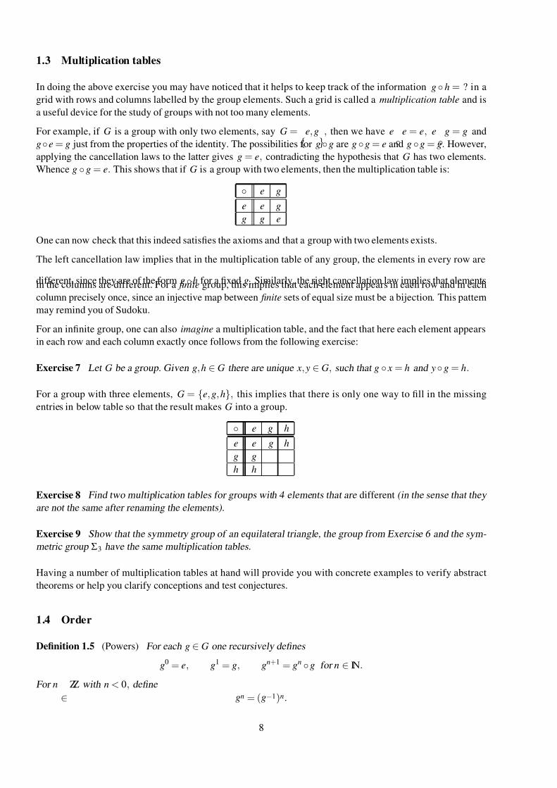
Whence g g = e. This shows that if G is a group with two elements, then the multiplication table is:
e g
e e g
g g e
One can now check that this indeed satisfies the axioms and that a group with two elements exists.
The left cancellation law implies that in the multiplication table of any group, the elements in every row are
different, since they are of the form g h for a fixed g. Similarly, the right cancellation law implies that elementsin the columns are different. For a finite group, this implies that each element appears in each row and in each
column precisely once, since an injective map between finite sets of equal size must be a bijection. This pattern
may remind you of Sudoku.
For an infinite group, one can also imagine a multiplication table, and the fact that here each element appears
in each row and each column exactly once follows from the following exercise:
Exercise 7 Let G be a group. Given g, h ∈ G there are unique x, y ∈ G, such that g x = h and y g = h.
For a group with three elements, G = e, g, h, this implies that there is only one way to fill in the missing
entries in below table so that the result makes G into a group.
e g h
e e g h
g g
h h
Exercise 8 Find two multiplication tables for groups with 4 elements that are different (in the sense that they
are not the same after renaming the elements).
Exercise 9 Show that the symmetry group of an equilateral triangle, the group from Exercise 6 and the sym-
metric group Σ3 have the same multiplication tables.
Having a number of multiplication tables at hand will provide you with concrete examples to verify abstract
theorems or help you clarify conceptions and test conjectures.
1.4 Order
Definition 1.5 (Powers) For each g ∈ G one recursively defines
g0 = e, g1 = g, gn+1 = gn g for n ∈ IN.
For n
∈ZZ with n < 0, define
gn = (g−1)n.
8
7/26/2019 MATH 2968 Algebra Advanced Notes
http://slidepdf.com/reader/full/math-2968-algebra-advanced-notes 9/110
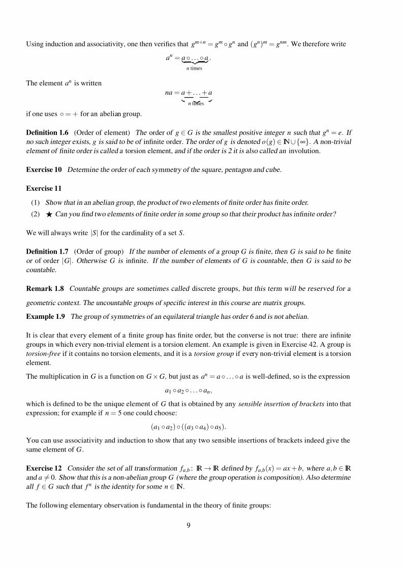
Using induction and associativity, one then verifies that gm+n = gm gn and (gn)m = gnm. We therefore write
an = a . . . a n times
.
The element an is written
na = a + . . . + a n times
if one uses = + for an abelian group.
Definition 1.6 (Order of element) The order of g ∈ G is the smallest positive integer n such that gn = e. If
no such integer exists, g is said to be of infinite order. The order of g is denoted o(g) ∈ IN∪∞. A non-trivial
element of finite order is called a torsion element, and if the order is 2 it is also called an involution.
Exercise 10 Determine the order of each symmetry of the square, pentagon and cube.
Exercise 11
(1) Show that in an abelian group, the product of two elements of finite order has finite order.
(2) Can you find two elements of finite order in some group so that their product has infinite order?
We will always write |S | for the cardinality of a set S .
Definition 1.7 (Order of group) If the number of elements of a group G is finite, then G is said to be finite
or of order |G|. Otherwise G is infinite. If the number of elements of G is countable, then G is said to be
countable.
Remark 1.8 Countable groups are sometimes called discrete groups, but this term will be reserved for a
geometric context. The uncountable groups of specific interest in this course are matrix groups.
Example 1.9 The group of symmetries of an equilateral triangle has order 6 and is not abelian.
It is clear that every element of a finite group has finite order, but the converse is not true: there are infinite
groups in which every non-trivial element is a torsion element. An example is given in Exercise 42. A group is
torsion-free if it contains no torsion elements, and it is a torsion group if every non-trivial element is a torsion
element.
The multiplication in G is a function on G × G, but just as an = a . . . a is well-defined, so is the expression
a1 a2 . . . an,
which is defined to be the unique element of G that is obtained by any sensible insertion of brackets into that
expression; for example if n = 5 one could choose:
(a1 a2) ((a3 a4) a5).
You can use associativity and induction to show that any two sensible insertions of brackets indeed give the
same element of G.
Exercise 12 Consider the set of all transformation f a,b : IR → IR defined by f a,b( x) = ax + b, where a, b ∈ IR
and a = 0. Show that this is a non-abelian group G (where the group operation is composition). Also determine
all f ∈ G such that f n is the identity for some n ∈ IN.
The following elementary observation is fundamental in the theory of finite groups:
9
7/26/2019 MATH 2968 Algebra Advanced Notes
http://slidepdf.com/reader/full/math-2968-algebra-advanced-notes 10/110
Exercise 13 Show that every finite group of even order contains an involution; i.e. if G is a finite group of
even order, then there is an element g ∈ G such that g = e = g2. Hint: g2 = e implies g−1 = g; try a counting
argument!
Example 1.10 (Dihedral group) The dihedral group Dn is the group of symmetries of a regular n –gon. This
has order 2n: there are n reflections and n rotations. (The identity is counted as a rotation with angle zero.)
The “degenerate cases” n = 1 and 2 are also included—try to find geometric objects that have D1 (identity and one reflection) and D2 (two rotations and two reflections) as symmetry groups.
Remark 1.11 (Order vs. action) The above dihedral group is often denoted D2n to emphasise its order rather
than the object it acts on.
1.5 Maps on groups
For a fixed h ∈ G, there are four important maps G → G:
(1) (left-multiplication by h) lh : G
→G, g
→hg
(2) (right multiplication by h ) r h : G → G, g → gh
(3) (conjugation by h) ch : G → G, g → h−1gh
(4) (orbit of h under conjugation) oh : G → G, g → ghg−1
Exercise 14 The multiplication maps and the conjugation map are bijections, and hence elements of Sym(G),but the last map may not be a bijection.
Much of group theory concerns the study of structure preserving maps between groups, which are called ho-
momorphisms. They will be studied in §3. However, we will also see that maps that are not homomorphisms
can be extremely useful.
1.6 Group actions
We have encountered some groups through the study of symmetries of certain objects, such as a triangle or a
square. This will now be formalised, and then studied in more detail in §6.
If X is a mathematical object with some structure, then a structure preserving bijection of X is a symmetry of
X , and the set of all of these structure preserving bijections of X is called the symmetry group of X . Notice the
subtle distinction: every symmetry of X is an element of the symmetric group Sym( X ), but not every element
of the symmetric group is a symmetry of X .
Definition 1.12 (Group action) An action of a group G on a mathematical object X is a map G × X → X ,written (g, x) → g · x, such that
(1) e · x = x for all x ∈ X ;
(2) (gh) · x = g · (h · x) for all g, h,∈ G and all x ∈ X .
We call this a G–action on X and say that G acts on X , written G X .
The set of symmetries of X can be studied without reference to X , and an understanding of its structure can lead
to new insights about X as well as new insights about other mathematical objects that have an equivalent set of
symmetries. Conversely, when one tries to understand a complicated group, whose structure is not so evident
from its algebraic description, one searches for mathematical objects on which this group acts in interesting
ways in order to coax some information about the group out of its action.
10
7/26/2019 MATH 2968 Algebra Advanced Notes
http://slidepdf.com/reader/full/math-2968-algebra-advanced-notes 11/110
Exercise 15 Show that the cube and the octahedron have the same group of symmetries.
In the above exercise, same can be interpreted more literally than comparing two multiplication tables: Both
the cube C and the octahedron O are subsets of IR3. Place them in IR3 in such a way that any symmetry
C → C extends to a map IR3 → IR3 that also takes O → O, and vice versa. The notion of same groups will be
formalised as isomorphic groups in §3.
Remark 1.13 More pedantically, the above definition should say left action, since the group elements act from
the left. There also is a notion of right action, where one has a map X × G → G satisfying:
(1) x · e = x for all x ∈ X ;
(2) x · (gh) = ( x · g) · h for all g, h,∈ G and all x ∈ X .
The notation for a left action matches our usual notation for composition of functions. You can compare this to
the discussion of the difference between reading elements of Σn from the left or right in §1.10.
1.7 Subgroups
We have already see examples of groups that naturally sit inside some bigger group, such as
SLn(ZZ) ⊂ SLn(IR) ⊂ SLn(C) ⊂ GLn(C).
The word “naturally” means that they are not just subsets, but the composition of two elements (thought of as
elements of the smaller group) is the same as their composition as elements of the bigger group. This is not the
case, for instance, with IR× ⊂ IR, because the composition in the former is multiplication whilst the latter is a
group with respect to addition.
Definition 1.14 (Subgroup) Let G be a group and U ⊆ G be a non-empty subset. If
(closure under multiplication) uv
∈U for all u, v
∈U , and
(closure under inversion) u−1 ∈ U for all u ∈ U ,
then U is a subgroup of G . We write U ≤ G.
I’ll emphasise the notation again: S ⊆ G is a subset , S ≤ G is a subgroup.
Since eG = uu−1 ∈ U for u ∈ U , it follows that U is a group with respect to the group operation of G. Any
group G has the subgroups eG and G. The subgroup U is proper if eU G.
Exercise 16 Determine whether r ∈ IR | r > 0 is a subgroup of IR×, and do the same for r ∈ IR | r < 0.
The following two exercises show how subgroups may help distinguish groups.
Exercise 17 (Quaternionic group) Define
1 =
1 0
0 1
, i =
0 −1
1 0
, j =
0 −i
−i 0
, k =
i 0
0 −i
.
(1) Show that the set Q8 = ±1,±i,± j,±k is closed under matrix multiplication—and hence a subgroup
of order 8 of GL(2,C).
(2) Determine all involutions in Q8.
(3) Show that Q8 has precisely 3 subgroups of order 4 and one subgroup of order 2.
Exercise 18 The dihedral group D4, the symmetry group of a square, has order 8. Show that D4 has precisely
3 subgroups of order 4 and 5 subgroups of order 2.
11
7/26/2019 MATH 2968 Algebra Advanced Notes
http://slidepdf.com/reader/full/math-2968-algebra-advanced-notes 12/110
1.8 Generating sets
Definition 1.15 (Generating set) If S ⊆ G is a subset, then define S −1 = s−1 | s ∈ S , and let S denote the
set of all elements of G which can be written as finite products of (not necessarily distinct) elements of S ∪S −1.
Lemma 1.16
S
is a subgroup of G , called the subgroup generated by S .
Definition 1.17 (Finitely generated) Let G be a group. Then G is finitely generated if there is a finite set
S ⊆ G such that G = S .
Every finite group is finitely generated; one can just take S = G. For many finite groups, nice generating sets
are known. For instance two standard generating sets for the symmetric group are:
Σn = (12), (123 · · ·n) = (12), (23), . . . , (n − 1 n).
Note that I write (12), (123 · · ·n) instead of (12), (123 · · ·n).
You know from the theory of vector spaces that every spanning set of a vector space contains a basis, and that
every vector space has a well-defined dimension, namely the cardinality of any basis. The generating sets forgroups do not allow an analogous theory. For instance,
ZZ = 1 = 2, 3 = 6, 10, 15,
but no proper subset of the second and third generating set generates ZZ.
Exercise 19 The additive group of rational numbers (Q, +) is not finitely generated. Hint: Find a normal
form for all elements that can be generated by a finite set in Q.
1.9 Cyclic groups
We now look at a class of groups that is particularly easy to understand, and which also shows how elementary
number theory can be used to study not only finite groups, but also infinite groups.
Definition 1.18 (Cyclic group) Let G be a group and g ∈ G. The subgroup g = gn | n ∈ ZZ ≤ G is called
the cyclic subgroup generated by g. If G = g for some g ∈ G, then G is called a cyclic group.
The definition of a cyclic group is worth paraphrasing: G is a cyclic group if there is an element g ∈ G such
that every element of G is a power of g, i.e. for each h ∈ G there is n ∈ ZZ such that h = gn. Examples of cyclic
groups are:
(1) ZZ =
1
=
−1
=
n
·1
|n
∈ZZ
(which is countably infinite);
(2) the group of rotations of a regular n–gon (which has order n);
(3) the group of all complex n–th roots of unity, i.e. the set of all complex numbers z such that zn = 1
(this also has order n ).
The following lemma follows from division with remainder:
Lemma 1.19 Let G be a group and g ∈ G.
(1) If o(g) = ∞, then gn = gm only if m = n.
(2) If o(g) < ∞, then gn = gm if and only if m ≡ n mod o(g). In particular, o(g) = |g|.
The Euclidean algorithm leads to the following result:
12
7/26/2019 MATH 2968 Algebra Advanced Notes
http://slidepdf.com/reader/full/math-2968-algebra-advanced-notes 13/110
Lemma 1.20 Every subgroup of a cyclic group is cyclic.
Exercise 20 Let n ∈ IN and for each r ∈ ZZ define
[r ] = r + nZZ = r + nk | k ∈ ZZ.
These are the congruence classes modulo n. Denote the set of all congruence classes modulo n by ZZn, and
define “addition” of congruence classes by:
[r ] [s] = (r + nZZ) (s + nZZ) = (r + s) + nZZ = [r + s].
Check that the operation is well defined and show that it turns ZZn into a group that is cyclic and of order n.We usually denote the operation on ZZn by +, writing [r ] + [s] = [r + s].
Exercise 21 Suppose G is a group and g ∈ G. Show that g = g−1. Is it always true that g = gn for
every n ∈ ZZ \0? If not, can you find conditions on n so that g = gn?
1.10 Symmetric and alternating groups
Recall that Σn = Sym(1, 2, . . . , n) is the symmetric group on n letters, and |Σn| = n!. A permutation f ∈ Σn
is a bijection f : 1, 2, . . . , n → 1, 2, . . . , n. A convenient notation to encode f is given by
f =
1 2 3 . . . n
f (1) f (2) f (3) . . . f (n)
.
The numbers in the top row are not always listed in ascending order. If n is fixed, one often omits all letters j
from the array which are fixed by the permutation. So we may write1 4 2
4 2 1
instead of
1 2 4
4 1 2
instead of
1 2 3 4 5
4 1 3 2 5
.
A k–cycle is a permutation f ∈Σn of the form
f =
a1 a2 a3 . . . ak −1 ak
a2 a3 a4 . . . ak a1
,
where a1, . . . , ak ∈ 1, 2, . . . , n are pairwise distinct. We also write the above k –cycle f in the form
f = (a1, a2, a3, · · · , ak ).
Note that we also have f = (a2, a3, a4, · · ·ak , a1). If n ≤ 9, we often omit the commata, so (123) = (1, 2, 3) ∈Σ3.A 2–cycle is called a transposition. The identity is often denoted (1).
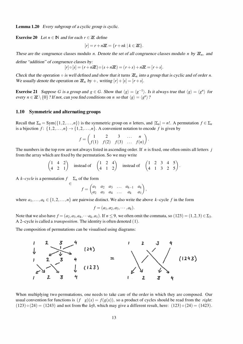
The composition of permutations can be visualised using diagrams:
When multiplying two permutations, one needs to take care of the order in which they are composed. Our
usual convention for functions is ( f
g)( x) = f (g( x)), so a product of cycles should be read from the right :
(123) (24) = (1243) and not from the left , which may give a different result, here: (123) (24) = (1423).
13
7/26/2019 MATH 2968 Algebra Advanced Notes
http://slidepdf.com/reader/full/math-2968-algebra-advanced-notes 14/110
The two different conventions illustrate a subtle point: they correspond precisely to the difference between left
actions and right actions.
In fancy language that will be introduced later (so you can ignore this sentence until you revise the notes for
the exam), the two actions are homomorphisms Σn → Σn, and the left action gives the trivial representation of
Σn to itself, whilst the other gives a conjugate representation.
Lemma 1.21 (Structure of permutations)
(1) The order of a k –cycle is k .
(2) Every element of Σn can be written as a product of disjoint cycles, called its cycle decomposition.
(3) Disjoint cycles commute.
(4) The order of an element of Σn is the least common multiple of the orders of the cycles in its cycle
decomposition.
(5) Every element of Σn can be written as a product of (not necessarily disjoint) transpositions. This product
is not unique, but the parity of the number of transpositions is unique. We accordingly call a permutation
even or odd.
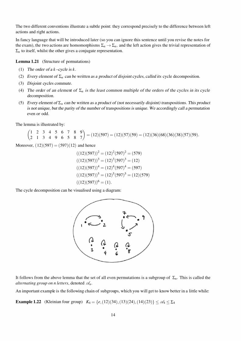
The lemma is illustrated by:1 2 3 4 5 6 7 8 9
2 1 3 4 9 6 5 8 7
= (12)(597) = (12)(57)(59) = (12)(36)(68)(36)(38)(57)(59).
Moreover, (12)(597) = (597)(12) and hence
((12)(597))2 = (12)2(597)2 = (579)
((12)(597))3 = (12)3(597)3 = (12)
((12)(597))4 = (12)4(597)4 = (597)
((12)(597))5 = (12)5(597)5 = (12)(579)
((12)(597))6 = (1).
The cycle decomposition can be visualised using a diagram:
It follows from the above lemma that the set of all even permutations is a subgroup of Σn. This is called the
alternating group on n letters, denoted A n.
An important example is the following chain of subgroups, which you will get to know better in a little while:
Example 1.22 (Kleinian four group) K 4 = e, (12)(34), (13)(24), (14)(23) ≤A 4 ≤ Σ4
14
7/26/2019 MATH 2968 Algebra Advanced Notes
http://slidepdf.com/reader/full/math-2968-algebra-advanced-notes 15/110
1.11 Summary
I have defined the concept of a group and given several key examples. I then indicated four ways of studying a
given group:
(1) via maps on the group;
(2) by getting the group to act on some mathematical object;(3) through an understanding of its subgroups; and
(4) via generating sets.
Each approach gives us a different angle on the group and often it is a combination that leads to a deeper
understanding of its structure. We will now develop these approaches and different ways of looking at them.
15
7/26/2019 MATH 2968 Algebra Advanced Notes
http://slidepdf.com/reader/full/math-2968-algebra-advanced-notes 16/110
2 Cosets
I’ll start this section with a brief review of equivalence relations and partitions. They will carry us through this
section, which is devoted to Lagrange’s theorem and a consequence in number theory. The last subsection gives
a nice geometric application of group theory.
2.1 Equivalence relations and partitions
Let S be a set and R ⊂ S × S . Define x ∼ y to mean ( x, y) ∈ R. Then ∼ is an equivalence relation if has the
following three properties:
(reflexive) x ∼ x for all x ∈ S ;
(symmetric) x ∼ y ⇐⇒ y ∼ x;
(transitive) x ∼ y and y ∼ z implies x ∼ z.
The equivalence class of x ∈ S is the set
[ x] = y
∈S
| y
∼ x ⊆
S .
The key properties of an equivalence relation are:
(1) [ x] = [ y] if and only if x ∼ y.
(2) [ x]∩ [ y] = / 0 if [ x] = [ y].
A partition of S is a collection of subsets of S , S k | k ∈ Λ, where Λ is an arbitrary index set, such that
S k ∩ S j = / 0 if k = j and S =
k ∈ΛS k .
Proposition 2.1 Let ∼ be an equivalence relation on the set S . Then the set of all equivalence classes
[ x] | x ∈ S is a partition of S . Conversely, for any partition of S there is an equivalence relation on S having the sets in the
partition as equivalence classes.
The set of all equivalence classes is usually denoted S / ∼ = [ x] | x ∈ S , and there is a canonical quotient map
p : S → S / ∼ defined by p( x) = [ x].
2.2 Cosets and index
Definition 2.2 (Cosets) Let G be a group and H ≤ G. A left coset of H in G is any set of the form
gH =
gh
|h
∈ H
for some g
∈G,
and a right coset of H in G is any set of the form
Hg = hg | h ∈ H for some g ∈ G.
Note that H = eH = He is always a left and right coset of itself. In general, gH = Hg. However, since the left
and right multiplication maps are bijections, we have |gH | = | H | = | Hg| for each g ∈ G.
Lemma 2.3 If H ≤ G, then an equivalence relation is defined on G by g ∼ h if and only if h−1g ∈ H .Moreover, the equivalence classes are the left cosets gH of H . Whence there is a partition of G of the form
G = j∈ J
g j H .
Moreover, the function aH → bH defined by ha → hb for h ∈ H is a bijection between aH and bH .
16
7/26/2019 MATH 2968 Algebra Advanced Notes
http://slidepdf.com/reader/full/math-2968-algebra-advanced-notes 17/110
Definition 2.4 (Index) The index of H in G is the number of left cosets of H in G, denoted |G : H |.
Example 2.5 Let G = Σ3 and H = (123). Then the cosets are H = (1), (123), (132) and (12) H =
(12), (23), (31). So |Σ3 : (123)| = 2.
Example 2.6 Let G = Σ3 and H = (12). Then the cosets are (1), (12), (123), (23), (132), (13). So
|Σ
3 : (12)| = 3.
Example 2.7 Let G = GL(2, IR) and H = SL(2, IR). Given any A ∈ G, the coset AH consists of matrices
having determinant equal to det( A). Moreover, any B ∈ G with det( B) = det( A) satisfies B ∈ AH , since B = A( A−1 B) and det( A−1 B) = 1. It follows that H has exactly one coset for each r ∈ IR×, so |G : H | = ∞.
Exercise 22 Show that |O(n)| = ∞= |SO(n)| if n ≥ 2, and |O(n) : SO(n)| = 2.
Example 2.8 Consider G = Dn and let H be the subgroup consisting of the n rotations (recall that the identity
is counted as a rotation). The left cosets are H and gH , where g is any reflection. This partitions Dn into the
rotations and the reflections, and the index of H is 2.
Exercise 23 The previous example leads to a normal form for elements of the dihedral group. Suppose a and b are symmetries of the regular n–gon, where a is a rotation by 2π /n and b is a reflection. Show that
an = e, b2 = e, bab−1 = bab = a−1.
Then show that every element of Dn has a unique expression of the form ak or bak , where k ∈ 0, . . . , n − 1.
Exercise 24 Let H be a subgroup of index 2 in G, and g, h ∈ G. If g /∈ H and h /∈ H , then gh ∈ H .
One can similarly formulate Definition 2.2 and Lemma 2.3 for right cosets. The index is the same, regardless
of which is chosen:
Exercise 25 Let G be a group and H
≤G. Suppose G can be written as a disjoint union:
G = j∈ J
g j H .
Then G can also be written as the following disjoint union:
G = j∈ J
Hg−1 j .
The discussion so far applies to finite and infinite groups, countable and uncountable groups.
2.3 Lagrange’s theorem
The two most fundamental results about finite groups, are considered to be Lagrange’s theorem and Sylow’stheorem. The former will be proved now, whilst the latter requires a better understanding of the structure of
finite groups.
Lagrange’s Theorem 2.9 Suppose G is a finite group and H ≤ G. Then | H | divides |G| and
|G| = |G : H | | H |.In particular, if g ∈ G, then the order of g divides |G|.
The converse of Lagrange’s theorem is not true in general. If G is finite and d divides |G|, then there may be
no subgroup of G of order d . However, a partial converse is given with Sylow’s theorem in §6.7.
Exercise 26 Let G be a group of order 841. If G is not cyclic, show that every element of G satisfies g29 = 1.
17
7/26/2019 MATH 2968 Algebra Advanced Notes
http://slidepdf.com/reader/full/math-2968-algebra-advanced-notes 18/110
2.4 Applications of Lagrange’s theorem
Corollary 2.10 If G is a finite group of order n = |G|, then gn = e for every g ∈ G
The following theorem from number theory (which is the basis of the RSA public key cryptosystem) follows
from the above.
Theorem 2.11 (Fermat’s little theorem) Let p be a prime number. If a is any integer which is not a multiple
of p, then
a p−1 ≡ 1 mod p.
Theorem 2.12 Let p be a prime number. Then every group of order p is cyclic.
2.5 The quaternions and the Hopf fibration
Here is a nice application of the basic fact that cosets partition a group, giving an application to an infinite
group.
Theorem 2.13 The 3–sphere S3 = x ∈ IR4 | | x| = 1 can be decomposed into pairwise disjoint unit circles.
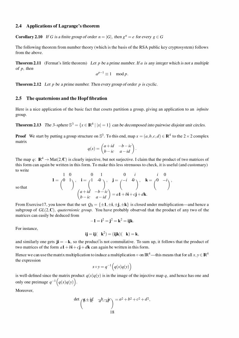
Proof We start by putting a group structure on S3. To this end, map x = (a, b, c, d ) ∈ IR4 to the 2×2 complex
matrix
q( x) =
a + id −b − ic
b − ic a − id
.
The map q : IR4 → Mat(2,C) is clearly injective, but not surjective. I claim that the product of two matrices of
this form can again be written in this form. To make this less strenuous to check, it is useful (and customary)
to write
1 = 1 0
0 1 , i = 0
−1
1 0 , j = 0
−i
−i 0 , k = i 0
0 −i ,
so that a + id −b − ic
b − ic a − id
= a1 + bi + c j + d k.
From Exercise17, you know that the set Q8 = ±1,±i,± j,±k is closed under multiplication—and hence a
subgroup of GL(2, C), quaternionic group. You have probably observed that the product of any two of the
matrices can easily be deduced from
−1 = i2 = j2 = k2 = ijk.
For instance,
ij = ij(
−k2) = (ijk)(
−k) = k,
and similarly one gets ji = −k, so the product is not commutative. To sum up, it follows that the product of
two matrices of the form a1 + bi + c j + d k can again be written in this form.
Hence we can use the matrix multiplication to induce a multiplication on IR4 —this means that for all x, y ∈ IR4
the expression
x y = q−1
q( x)q( y)
is well-defined since the matrix product q( x)q( y) is in the image of the injective map q, and hence has one and
only one preimage q−1
q( x)q( y)
.
Moreover,
deta + id −b − icb − ic a − id = a2 + b2 + c2 + d 2,
18
7/26/2019 MATH 2968 Algebra Advanced Notes
http://slidepdf.com/reader/full/math-2968-algebra-advanced-notes 19/110
so the matrix is invertible if and only if (a, b, c, d ) = (0, 0, 0, 0) = 0 ∈ IR4, and we get a group structure on
IR4 \ 0. Since the determinant satisfies det( AB) = det( A) det( B) and det( A−1) = (det( A))−1, it follows that
q(S3) is a subgroup of SL2(C), and hence (S3,) is a subgroup of (IR4 \0,).
A simple computation shows that H = (cosϑ )1 + (sinϑ )i) | ϑ ∈ IR corresponds to a subgroup of q(S3).Moreover q−1( H ) is a unit circle in the usual xy–plane in IR4 . The cosets q( x) H , where x ∈ S3, partition
q(S3) by Lemma 2.3. One can now verify that the preimage of each coset again is a unit circle—either by
a direct computation or by noticing that the unit quaternions correspond to rotations of IR4 fixing the origin
(just as the unit complex numbers act as rotations of the plane fixing the origin). The decomposition into these
circles is called the Hopf fibration.
2.6 Summary
We partitioned a group using cosets of a fixed subgroup, and used the partition to study the group. For finite
groups, this gives a complete understanding of the possible orders of subgroups and, in particular, of the possible
orders of elements. In the last subsection, you have seen how an injective map from a given set S to a group G
can be used to give the set S the structure of a group in order to obtain more information about it. This is a key
technique not only in geometry or algebra, but also in physics.
19
7/26/2019 MATH 2968 Algebra Advanced Notes
http://slidepdf.com/reader/full/math-2968-algebra-advanced-notes 20/110
3 Homomorphisms, normal subgroups and quotient groups
This section is devoted to the study of structure preserving maps between groups. It turns out that they have
many wonderful, powerful properties that lay the foundation for everything else to come.
3.1 Homomorphisms
Definition 3.1 (Homomorphism) Let (G,G) and ( H , H ) be groups. A map ϕ : G → H is a homomorphism
if
ϕ (a G b) = ϕ (a) H ϕ (b)
for all a, b ∈ G. A surjective homomorphism ϕ is called an epimorphism, an injective homomorphism is a
monomorphism, and a bijective homomorphism is an isomorphism. If there is an isomorphism between G and
H , then the groups are called isomorphic, written G ∼= H .
Exercise 27 If ϕ : G → H is a homomorphism, then for each g ∈ G we have ϕ (g−1) = (ϕ (g))−1 and ϕ (eG) =e H .
An epimorphism is often indicated by ϕ : G H , a momomorphism by ϕ : G → H and an isomorphism by
ϕ : G ∼= H .
Exercise 28 Several groups have been shown to be the “same” in previous exercises. Check that “same”
means “isomorphic.” Also show that your two groups of order 4 from Exercise 8 are not isomorphic.
Remark 3.2 It is understood that for elements of G, we use the group operation G defined on G and likewise
H is used for elements of H . We therefore simply write ϕ (a b) = ϕ (a) ϕ (b) or ϕ (ab) = ϕ (a)ϕ (b).
Example 3.3 The determinant det: GL(n, F )
→F × is a homomorphisms since det( AB) = det( A) det( B). It
is an epimorphism, since for any f ∈ F ×, one can take the diagonal matrix with precisely one entry equal to f and all other entries equal to 1, giving an element of GL(n, F ) with determinant f . Permuting the diagonal
entries, one sees that det is injective (if and) only if n = 1.
Example 3.4 The exponential function gives an isomorphism between (IR, +) and (IR>0,×). The inverse of
this isomorphism is the natural logarithm.
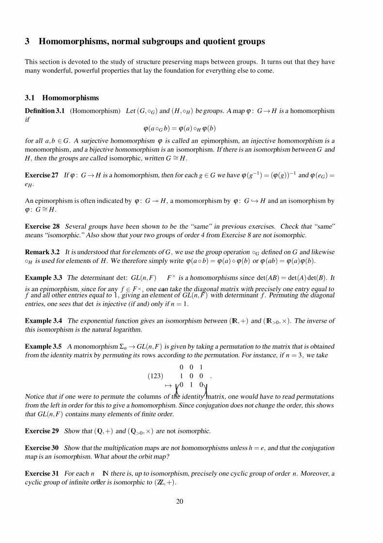
Example 3.5 A monomorphism Σn → GL(n, F ) is given by taking a permutation to the matrix that is obtained
from the identity matrix by permuting its rows according to the permutation. For instance, if n = 3, we take
(123)
→0 0 1
1 0 0
0 1 0 .
Notice that if one were to permute the columns of the identity matrix, one would have to read permutations
from the left in order for this to give a homomorphism. Since conjugation does not change the order, this shows
that GL(n, F ) contains many elements of finite order.
Exercise 29 Show that (Q, +) and (Q>0,×) are not isomorphic.
Exercise 30 Show that the multiplication maps are not homomorphisms unless h = e, and that the conjugation
map is an isomorphism. What about the orbit map?
Exercise 31 For each n∈
IN there is, up to isomorphism, precisely one cyclic group of order n. Moreover, a
cyclic group of infinite order is isomorphic to (ZZ, +).
20
7/26/2019 MATH 2968 Algebra Advanced Notes
http://slidepdf.com/reader/full/math-2968-algebra-advanced-notes 21/110
As an abstract group, the cyclic group of order n will be denoted
C n = g | gn = e.
An expression of this form is called a group presentation. We will work with group presentations in an informal
way in this course; a proper treatment is in §9.2.
Exercise 32 (Homomorphism determined by generators) Let G and H be groups. Suppose S = g0, . . . , gnis a generating set for G. Suppose ϕ : G → H and ψ : G → H are homomorphisms with the property that
ϕ (gk ) = ψ (gk ) for all k ∈ 0, . . . n. Show that ϕ = ψ .
Exercise 33 Show that there is a monomorphism Dm → Dn if m divides n.
3.2 Kernel and image
Definition 3.6 (Kernel and image) If ϕ : G → H is a homomorphism, define
ker(ϕ ) =
g
∈G
|ϕ (g) = e H
⊆G and im(ϕ ) =
ϕ (g)
|g
∈G
⊆ H .
Example 3.7 Consider the homomorphism det: GL(n, F ) → F ×. We have im(det) = F × and
ker(det) = A ∈ GL(n, F ) | det A = 1 = SL(n, F ).
Exercise 34 Let G and H be groups and suppose ϕ : G → H is a homomorphism. Then im(ϕ ) ≤ H and
ker(ϕ ) ≤ G.
Lemma 3.8 Let G and H be groups and suppose ϕ : G → H is a homomorphism. Then ϕ is injective if and
only if ker(ϕ ) = eG.
Kernel and image have the following natural generalisations:
Exercise 35 Let G and H be groups and suppose ϕ : G → H is a homomorphism.
(1) (Image of subgroup is subgroup) If U ≤ G, then ϕ (U ) ≤ H .
(2) (Preimage of subgroup is subgroup) If V ≤ H , then g ∈ G | ϕ (g) ∈ V ≤ G.
The kernel of ϕ is the preimage of the trivial group, and the image of ϕ is the image of the whole group.
The kernel has some special structure, which we turn to next.
3.3 Normal subgroups
Definition 3.9 (Normal subgroup) Let G be a group and U ≤ G be a subgroup. If g−1ug ∈ U for all u ∈ U
and all g ∈ G, then U is called a normal subgroup of G, written U G.
Exercise 36 Let H denote the subset of GL(2, IR) consisting of all upper triangular matrices. Show that H is a
subgroup of GL(2, IR). Then consider the subset N of all upper triangular matrices having 1’s on the diagonal.
Show that N H . Is it also the case that N G?
The trivial group e and the whole group are always normal subgroups of G.
Exercise 37 Every subgroup of an abelian group is normal.
21
7/26/2019 MATH 2968 Algebra Advanced Notes
http://slidepdf.com/reader/full/math-2968-algebra-advanced-notes 22/110
An important example of a normal subgroup is the following:
Lemma 3.10 Let G and H be groups and suppose ϕ : G → H is a homomorphism. Then ker(ϕ )G.
It is useful to generalise the definition of a coset to multiplication of subsets of G. For A, B ⊆ G, define the set
AB = ab | a ∈ A, b ∈ B ⊆ G.Since the group operation is associative, the same is true for multiplications of subsets, and hence we can write
ABC = ( AB)C = A( BC ). If a set contains only a single element, e.g. B = g we also write ABC = AgC .
Lemma 3.11 Suppose G is a group and H ≤ G. The following are equivalent:
(1) H G
(2) For all g ∈ G we have gH = Hg.
(3) For all g ∈ G we have g−1 Hg = H .
Exercise 38 Let G be a group and H
≤G with
|G : H
|= 2. Then gH = Hg for all g
∈G and hence H G.
Exercise 39 Let H 1 and H 2 be subgroups of the group G, and define the set
H 1 H 2 = h1h2 | hk ∈ H k .
(1) H 1 H 2 is a subgroup of G if and only if H 1 H 2 = H 2 H 1.
(2) Suppose H ≤ G and N G. Then HN = NH and hence HN = NH ≤ G.
(3) Let N 1G and N 2G. Then:
N 1 N 2G and N 1 ∩ N 2G.
(4) If H 1 and H 2 are finite subgroups of G then (regardless of whether H 1 H 2 is a subgroup or not) we have
| H 1 H 2| = | H 1| | H 2|| H 1 ∩ H 2| .
Exercise 40 This exercise continues the study of Q8 and D4 from Exercises 17 and 18 respectively.
(1) Show that every subgroup of Q8 is a normal subgroup of Q8.
(2) Which subgroups of D4 are normal in D4 ?
(3) Find subgroups H 1 and H 2 of D4 with H 1 H 2 D4, but H 1 is not normal in D4.
Remark 3.12 Non-abelian groups with the property that all subgroups are normal are called Hamiltonian
groups. The finite Hamiltonian groups were classified by Dedekind, and this classification was extended to all groups by Baer. The details are given in 9.7.4 in [19], and this proof should be accessible after §6.
3.4 Quotient group
We now show that, conversely, every normal subgroup is the kernel of some homomorphism. It is instructive to
check why the proof of the below lemma does not work for general subgroups, but only for normal subgroups.
A simple application of Lemma 3.11 shows that the product of any two cosets of a given normal subgroup is
always a coset of that normal subgroup:
Lemma 3.13 Suppose N G. Then (gN )(hN ) = (gh) N .
22
7/26/2019 MATH 2968 Algebra Advanced Notes
http://slidepdf.com/reader/full/math-2968-algebra-advanced-notes 23/110
Proposition 3.14 (Quotient group) Suppose N G. Consider the set of all left cosets of N , written
G/ N = gN | g ∈ G.
Define the operation
gN hN = (gh) N .
Then this is well-defined and turns G/ N into a group with the identity element N . Moreover, the map g
→gN
defines an epimorphism G → G/ N with kernel equal to N .
Exercise 41 Show that there are a group G and a subgroup H ≤ G, such that the set of all left cosets of H is
not a group using the operation gH hH = (gh) H .
Example 3.15 Let nZZ = nk | k ∈ ZZ = . . . ,−2n,−n, 0, n, 2n, . . .. This is a subgroup of ZZ and hence
normal since ZZ is abelian. The quotient group ZZ/nZZ is a finite cyclic group of order n. The equivalence
relation defining the cosets is precisely congruence modulo n, and hence ZZ/nZZ = ZZn.
Example 3.16 Consider SL(n, F ) ≤ GL(n, F ). Given any A ∈ GL(n, F ) and B ∈ SL(n, F ), we have
det( A−1
BA) = det( A−1
) det( B) det( A) = (det( A))−1
det( A) = 1
and so A−1 BA ∈ SL(n, F ). Since A and B were arbitrary, this shows that SL(n, F )GL(n, F ). A coset is of
the form B SL(n, F ), where B ∈ GL(n, F ). For any C ∈ B SL(n, F ), we have detC = det B. Conversely, if
detC = det B for some C ∈ GL(n, F ), then det( B−1C ) = 1 and so C = ( BB−1)C = B( B−1C ) ∈ B SL(n, F ). This
shows that there is a well-defined bijection between cosets of SL(n, F ) and elements of F × given by
ϕ ( B SL(n, F )) = det( B).
Using the multiplicative property of the determinant, one sees that this bijection is in fact an isomorphism:
ϕ ( B SL(n, F ))ϕ (C SL(n, F )) = det( B) det(C ) = det( BC ) = ϕ ( BC SL(n, F )).
At first sight, the quotient group GL(n, F )/SL(n, F ) may seem unwieldy, but the isomorphism with F × makes
it easy to work with.
A consequence of Lagrange’s theorem is that for a finite group G, |G/ N | = |G|| N | .
Example 3.17 Consider the group D4 = a, b | a4 = e, b2 = e, bab = a−1 and the subgroup N = a2. Since
a−1(a2)a = a2 ∈ N and b−1(a2)b = (bab)(bab) = a−2 ∈ N , the subgroup N is normal in D4. (Why?) Now
| D4/ N | = | D4|| N | =
8
2 = 4,
so there are two possibilities for the isomorphism type of the quotient group. Computing the cosets
N = e, a2, aN = a, a3, bN = b, ba2, baN = ba, ba3,
allows us to determine the multiplication table:
N aN bN baN
N N aN bN baN
aN aN N baN bN
bN bN baN N aN
baN baN bN aN N
From this we see D4/ N ∼= K 4.
Exercise 42 Show that Q/ZZ is an infinite torsion group.
23
7/26/2019 MATH 2968 Algebra Advanced Notes
http://slidepdf.com/reader/full/math-2968-algebra-advanced-notes 24/110
3.5 More applications of Lagrange’s theorem
The heading of this subsection may be slightly misleading as Lagrange’s theorem is a result about finite groups
(at least in the version stated in these notes).
Exercise 43 Let G be a group, and H 1 and H 2 be subgroups of finite index of G, i.e. |G : H 1| < ∞ and
|G : H 2| < ∞.(1) Then
|G : H 1 ∩ H 2| ≤ |G : H 1| |G : H 2|.(2) If G is a finite group, then
|G : H 1 ∩ H 2| = |G : H 1| |G : H 2|if and only if G = H 1 H 2.
(3) If G is a finite group and |G : H 1| and |G : H 2| are coprime, then G = H 1 H 2.
Example 3.18 Let G = ZZ, and consider its subgroups A = 6ZZ, B = 8ZZ and C = 5ZZ. Then A ∩ B = 24ZZ
and A∩
C = 30ZZ. We therefore have:
|G : A ∩ B| = 24 < 6 · 8 = |G : A| |G : B|.and
|G : A ∩C | = 30 = 6 · 5 = |G : A| |G : C |.
Exercise 44 Let G be a finite group, H ≤ G and N G.
(1) If | H | and |G/ N | are coprime, then H ≤ N .
(2) If | N | and |G : H | are coprime, then N ≤ H . (Hint: compute | NH |.)
3.6 Simple groups
If e and G are the only normal subgroups of G, then G is termed simple. If a group is not simple, then
one can understand its structure via the normal subgroup N and the quotient group G/ N . If the group G is
finite, then this gives two groups of smaller order and hence one can inductively repeat this process until all
groups involved are finite simple groups. The finite simple groups can be viewed as building blocks from which
all other finite groups can be constructed (akin to the prime numbers giving all whole numbers); this is made
precise in §3.8. The classification of finite simple groups is one of the great milestones in mathematics (and its
proof fills over 10,000 pages and is still being simplified).
A finite simple group belongs to one of 18 infinite families, or it is one of the 26 so-called sporadic groups.
The only simple abelian groups are the cyclic groups of prime order; they form the first of the 18 families.
All other finite simple groups are non-abelian and have even order due to a result by Feit and Thompson(see Remark 5.24). You have already proven that every group of even order contains an involution, and the
involutions play a special role in the study of the sporadic finite simple groups.
The second infinite family of finite simple groups are the alternating groups A n for n ≥ 5.
Theorem 3.19 The alternating groups A n for n ≥ 5 are simple.
The theorem follows from the following three lemmata (why?), and you can find the proofs in [1], §2.9.4.
Lemma 3.20 Every permutation in A n is a product of 3–cycles if n ≥ 3.
Lemma 3.21 Given an 3–cycle (abc) ∈A n, n ≥ 3, there is an element g ∈A n such that g−1(abc)g = (123).
24
7/26/2019 MATH 2968 Algebra Advanced Notes
http://slidepdf.com/reader/full/math-2968-algebra-advanced-notes 25/110
Lemma 3.22 A non-trivial normal subgroup of A n must contain a 3–cycle if n ≥ 5.
The group A5 of order 60 is the unique smallest non-abelian simple group; this fact can be proved with the
material of §6.
Exercise 45 The only proper normal subgroup of Σn is A n for n = 4.
Exercise 46 Show that K 4 is normal in both A 4 and Σ4.
It follows from the exercise that the group A 4 is not simple since it has the Klein four group as a normal
subgroup. This is the conceptual reason of why one can write the solutions to equations of the form
xn + an−1 xn−1 + . . . + a2 x
2 + a1 x + a0 = 0
with n ≤ 4 using square roots, whilst this is not possible if n ≥ 5.
3.7 The isomorphism theorems
The proof of the following theorem formalises various examples that were given in the previous sections.
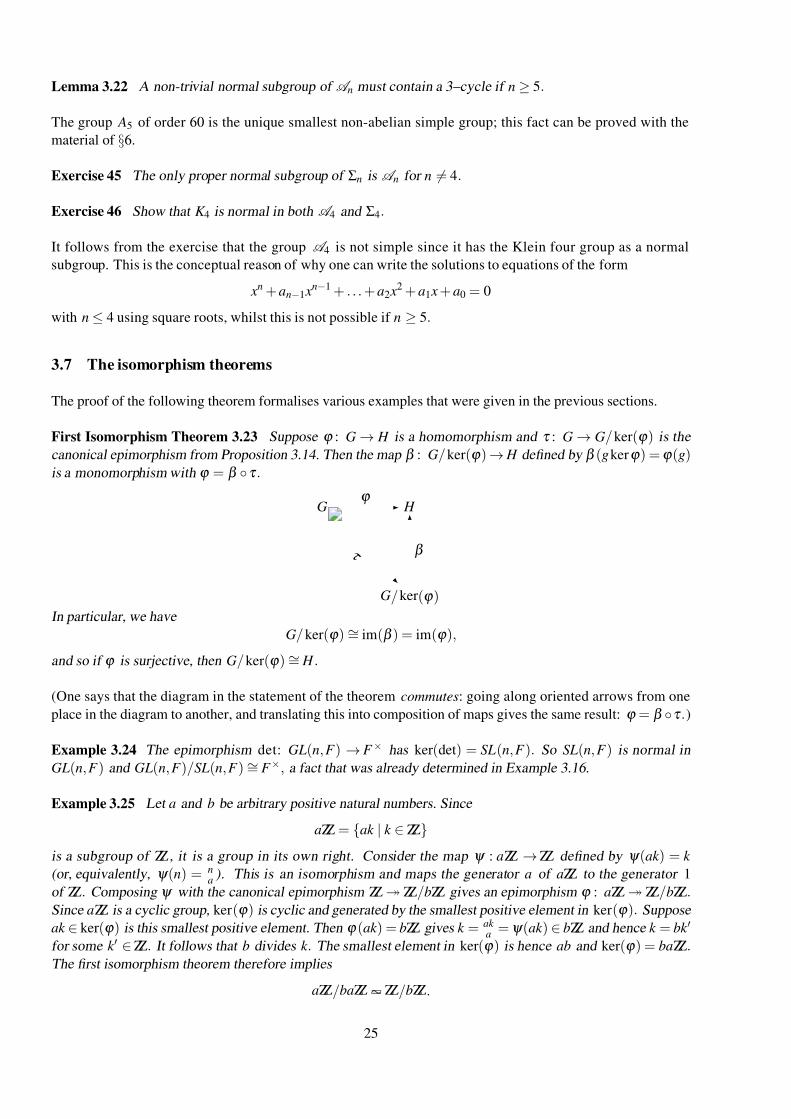
First Isomorphism Theorem 3.23 Suppose ϕ : G → H is a homomorphism and τ : G → G/ ker(ϕ ) is the
canonical epimorphism from Proposition 3.14. Then the map β : G/ ker(ϕ ) → H defined by β (g kerϕ ) =ϕ (g)is a monomorphism with ϕ = β τ .
Gϕ H
τ
G/ ker(ϕ )
β
In particular, we have
G/ ker(ϕ ) ∼= im(β ) = im(ϕ ),
and so if ϕ is surjective, then G/ ker(ϕ ) ∼= H .
(One says that the diagram in the statement of the theorem commutes: going along oriented arrows from one
place in the diagram to another, and translating this into composition of maps gives the same result: ϕ = β τ .)
Example 3.24 The epimorphism det: GL(n, F ) → F × has ker(det) = SL(n, F ). So SL(n, F ) is normal in
GL(n, F ) and GL(n, F )/SL(n, F ) ∼= F ×, a fact that was already determined in Example 3.16.
Example 3.25 Let a and b be arbitrary positive natural numbers. Since
aZZ = ak | k ∈ ZZis a subgroup of ZZ , it is a group in its own right. Consider the map ψ : aZZ → ZZ defined by ψ (ak ) = k
(or, equivalently, ψ (n) = na
). This is an isomorphism and maps the generator a of aZZ to the generator 1
of ZZ. Composing ψ with the canonical epimorphism ZZ ZZ/bZZ gives an epimorphism ϕ : aZZ ZZ/bZZ.Since aZZ is a cyclic group, ker(ϕ ) is cyclic and generated by the smallest positive element in ker(ϕ ). Suppose
ak ∈ ker(ϕ ) is this smallest positive element. Then ϕ (ak ) = bZZ gives k = ak a
= ψ (ak ) ∈ bZZ and hence k = bk
for some k ∈ ZZ. It follows that b divides k . The smallest element in ker(ϕ ) is hence ab and ker(ϕ ) = baZZ.The first isomorphism theorem therefore implies
aZZ/baZZ ∼= ZZ/bZZ.
25
7/26/2019 MATH 2968 Algebra Advanced Notes
http://slidepdf.com/reader/full/math-2968-algebra-advanced-notes 26/110
Exercise 47 Suppose ϕ : G H is an epimorphism with kernel N . For any subgroup F of G, ϕ (F ) is
a subgroup of H . Show that this map gives a bijection between the subgroups of G containing N and the
subgroups of H . Furthermore, for these subgroups we have F G if and only if ϕ (F ) H .
Important applications of the first isomorphism theorem are the second and the third isomorphism theorems.
As with the first, they manifest themselves naturally in examples, and they give important constructions that
should become second nature.
Second Isomorphism Theorem 3.26 Let G be a group, H ≤ G and N G. Then H N is a subgroup of G and
the map ϕ : H → ( HN )/ N defined by ϕ (h) = hN is an epimorphism with kerϕ = H ∩ N . We therefore have
( H ∩ N ) H and
( HN )/ N ∼= H /( H ∩ N ).
Example 3.27 Take G = ZZ, and use additive notation for the group operation. Define H = 6ZZ = 6k | k ∈ ZZand N = 9ZZ = 9k | k ∈ ZZ. Then H and N are subgroups of G and since every subgroup of an abelian group
is normal, we have N G. We have:
H + N = 6k 1 + 9k 2 | k 1, k 2 ∈ ZZ= 3 (2k 1 + 3k 2) | k 1, k 2 ∈ ZZ= 3k | k ∈ ZZ= 3ZZ,
where the third equality can be seen as follows. The inclusion 3 (2k 1 + 3k 2) | k 1, k 2 ∈ ZZ ⊆ 3ZZ is clear. The
reverse follows by letting k 1 = −1 and k 2 = 1. Thus, 3(−2 + 3) = 3 is contained in the subgroup
H + N = 3 (2k 1 + 3k 2) | k 1, k 2 ∈ ZZand hence 3ZZ = 3 ⊆ H + N . We also have:
H
∩ N =
k
∈ZZ
|k = 6k 1 and k = 9k 2 for some k 1, k 2
∈ZZ
= 18k | k ∈ ZZ= 18ZZ.
Now Example 3.25 gives:
H /( H ∩ N ) = 6ZZ/18ZZ ∼= ZZ/3ZZ ∼= 3ZZ/9ZZ = ( H + N )/ N ,
as predicted by the second isomorphism theorem.
Example 3.28 The above example is generalised as follows. In G = ZZ consider the subgroup H = hZZ =hk | k ∈ ZZ and the normal subgroup N = nZZ = nk | k ∈ ZZ. We need a little help from elementary number
theory: if p and q are coprime integers, then there are integers r and s such that ps−
qr = 1. Using this, one
obtains:
H + N = gcd(h, n)ZZ, and H ∩ N = lcm(h, n)ZZ,
where gcd is the greatest common divisor and lcm is the least common multiple. The second isomorphism
theorem gives:
ZZ/ n
gcd(h, n)ZZ ∼= gcd(h, n)ZZ/nZZ ∼= ( H + N )/ N ∼= H /( H ∩ N ) ∼= hZZ/ lcm(h, n)ZZ ∼= ZZ/
lcm(h, n)
h ZZ.
Since ZZ/aZZ ∼= ZZ/bZZ if and only if a = b, this shows that for any two natural numbers h and n :
nh = gcd(h, n) lcm(h, n).
The next theorem is reminiscent of the division of rational numbers.
26
7/26/2019 MATH 2968 Algebra Advanced Notes
http://slidepdf.com/reader/full/math-2968-algebra-advanced-notes 27/110
Third Isomorphism Theorem 3.29 Let G be a group, N G and K G with K ≤ N . Then the map
ϕ : G/K → G/ N defined by ϕ (gK ) = gN is an epimorphism with kerϕ = N /K . We therefore have N /K G/K
and
(G/K )/( N /K ) ∼= G/ N .
Example 3.30 You know that K 4A 4Σ4 and K 4Σ4. Just looking at the orders gives Σ4/A 4 ∼= C 2 and
A 4/K 4 ∼= C 3. However, we need to identify Σ4/K 4 (a group of order 6) and
A 4/K 4 as a subgroup of this.
One can identify Σ4 with the group of rotational symmetries of a cube, with the four letters being permuted
being the four diagonals of the cube. The transpositions correspond to non-trivial rotations by π about lines
through the midpoints of opposite edges. The 3–cycles correspond to rotations by 2π /3 about lines through
opposite vertices. The 4–cycles correspond to rotations by 2π /4 about lines through the midpoints of opposite
faces, and the elements of the Klein four group to rotations by π about these lines.
One can now define an epimorphism Σ4 → Σ3 by taking a rotation to the corresponding permutation of the set
of the three lines through the midpoints of opposite faces. The kernel of this epimorphism is K 4, so by the
first isomorphism theorem we have Σ4/K 4 ∼= Σ3. This also gives A 4/K 4 ∼= A 3. Hence the third isomorphism
theorem gives the familiar fact:
Σ3/A
3 ∼= (Σ4/K 4)/(A
4/K 4) ∼= Σ4/A
4 ∼= C 2.
3.8 The Jordan-H older theorem
This section shows that some groups (including all finite groups) have a unique factorisation into simple groups.
This should be read literally: we only divide a group into smaller groups. Multiplying groups to give new groups
will be done in the next section.
A chain of subgroups G = G0 ≥ G1 ≥ G2 ≥ . . . ≥ Gn = 1 is called a normal series of G if Gk Gk −1 for
each 1 ≤ k ≤ n. The quotient groups Gk −1/Gk are the factors of the normal series and the length of the normal
series is the number of strict inclusions (i.e. the number of non-trivial factors). The length is therefore bounded
above by n, but may be strictly less.
If N G, then N is a maximal proper normal subgroup if N < G and there is no normal subgroup H G such
that N < H < G, where < denotes strict inclusion. It follows from Exercise 47 that G/ N is a non-trivial simple
group if and only if N is a maximal proper normal subgroup of G.
In contrast, a subgroup H ≤ G is a maximal proper subgroup if H < G and there is no subgroup K ≤ G such
that H < K < G. So it could happen that a maximal proper normal subgroup is not a maximal proper subgroup.
However, in an abelian group these notions coincide since every subgroup is normal.
Going back to the above normal series, if for each k , either Gk is a maximal proper normal subgroup of Gk −1 or
Gk = Gk −1, then the normal series is called a composition series. So each factor Gk −1/Gk is a (possibly trivial)
simple group; the non-trivial factors are called the composition factors. The possibility Gk = Gk −1 is allowed
to make some of below proofs less verbose. If it is never the case that Gk = Gk −
1, then the composition series
is said to be without repetitions. Deleting repeated subgroups results in a composition series without repetitions
having the same length and the same non-trivial factors.
Example 3.31 For n = 4, the alternating group A n is the only non-trivial normal subgroup of Σn, and A n is
simple. So there is a unique composition series without repetitions for Σn :
Σn ≥A n ≥ e.
The factors of this series are Σn/A n ∼= C 2 and A n/e ∼=A n and its length is 2. Any other composition series
is obtained by repeating some of the above groups, such as:
Σn ≥ Σn ≥A n ≥A n ≥A n ≥ e.
The factors of this series are Σn
/Σn ∼
=
e
, Σn
/A n ∼
= C 2, A
n/A
n ∼=
e
, A n
/A n ∼
=
e
, A n
/
e ∼
= A n
, and
since only two of the factors are non-trivial, its length is again 2.
27
7/26/2019 MATH 2968 Algebra Advanced Notes
http://slidepdf.com/reader/full/math-2968-algebra-advanced-notes 28/110
Exercise 48 Every finite group has a composition series. Moreover, the product of the orders of the composi-
tion factors of a finite group equals the order of the group.
Exercise 49 Show that the quaternion group Q8 has three composition series without repetitions.
Exercise 50 An abelian group has a composition series if and only if it is finite. (Hint: think about ZZ
first.)
Example 3.32 The only maximal normal subgroup of Σ4 is A 4, and the latter also has a unique maximal
normal subgroup, namely K 4. Now K 4 has three maximal normal subgroups (each isomorphic with C 2 ) giving
three composition series (without repetitions) for Σ4 :
Σ4 ≥A 4 ≥ K 4 ≥ (12)(34) ≥ e,
Σ4 ≥A 4 ≥ K 4 ≥ (13)(24) ≥ e,
Σ4 ≥A 4 ≥ K 4 ≥ (14)(24) ≥ e.
All series have length 4 and the factors Σ4/A 4 ∼= C 2, A 4/K 4 ∼= C 3, K 4/(ab)(cd ) ∼= C 2 and C 2/e ∼= C 2.
The Jordan-Holder theorem asserts that the non-trivial factors that arise in one composition series of a groupcan always be matched up with the non-trivial factors that arise in another composition series of the same group,
but the order in which they occur may change. Here is an example of this phenomenon.
Example 3.33 The group C 12 has the following three composition series with associated sequences of factors:
1C 2C 4C 12 with sequence C 2,C 2,C 3;
1C 2C 6C 12 with sequence C 2,C 3,C 2;
1C 3C 6C 12 with sequence C 3,C 2,C 2.
The pieces of the Jordan-Holder theorem are, as the name suggests, due to Jordan (1868) and H older (1889).
The modern proof follows Schreier (1928) with simplifications by Zassenhaus (1934). The following language
is useful:
Definition 3.34 Two normal series of a group are equivalent if there is a bijection between their non-trivial
factor groups such that corresponding factors are isomorphic.
It follows from the definition that equivalent normal series have the same length.
The idea of the proof of the Jordan-Holder theorem is to take one composition series and to insert a full copy
of the second composition series between any two members of the first series, and vice versa. Since both
series are composition series, this merely inserts repetitions of elements, and hence does not change any of the
composition factors. The factors are matched up in isomorphic pairs using the following result, which follows
from the isomorphism theorems:
Zassenhaus Lemma 3.35 Suppose A1, A2, B1, B2 are subgroups of the group G with A2 A1 and B2 B1.
Then
A2( A1∩ B1)/ A2( A1∩ B2) ∼= B2( B1∩ A1)/ B2( B1∩ A2)
The normal series
G = H 0 ≥ H 1 ≥ H 2 ≥ . . . ≥ H m = 1is a refinement of the normal series
G = G0
≥G1
≥G2
≥. . .
≥Gn =
1
if G0, G1, G2, . . . , Gn is a subsequence of H 0, H 1, H 2, . . . , H m.
28
7/26/2019 MATH 2968 Algebra Advanced Notes
http://slidepdf.com/reader/full/math-2968-algebra-advanced-notes 29/110
Schreier Refinement Theorem 3.36 Suppose G is a (possibly infinite) group which has a normal series. Any
two normal series of G have refinements that are equivalent.
With the above results, the proof of the main theorem is a breeze:
Jordan-H older Theorem 3.37 Suppose G is a (possibly infinite) group which has a composition series. Then
any two composition series of G are equivalent, i.e. they have the same length and, with respect to a suitable reordering of the non-trivial composition factors, the corresponding factors are isomorphic.
Corollary 3.38 (Fundamental Theorem of Arithmetic) Every integer greater than one has a unique factorisa-
tion into prime numbers.
Example 3.39 It follows from the (proof of the) above corollary that the composition factors of a cyclic group
of order 24 = 23 ·3 are the same as the composition factors of Σ4. Whence the conclusion of the Jordan-H older
theorem holds for any two composition series of Σ4 and C 24 even though the two groups are not isomorphic.
Before we study composition series for abelian groups in more detail in
§5.2, we need to be able to see more
structure in a group. In particular, we need to be able to multiply groups in a meaningful way.
3.9 Summary
The material of this section will be our bread and butter for the remainder of the semester. The interplay between
homomorphisms, normal subgroups and quotient groups is fundamental to group theory and its applications.
In the last section, a new idea for the study of groups was introduced, namely the study of chains of subgroups
inside the group. The proof of the Jordan-Holder theorem uses most of the tools at our current disposal.
29
7/26/2019 MATH 2968 Algebra Advanced Notes
http://slidepdf.com/reader/full/math-2968-algebra-advanced-notes 30/110
4 Direct and semi-direct products
This section first continues our study of a group via its subgroups by introducing two subgroups that are char-
acteristic: its centre and its commutator subgroup. We then attach another group to a group: namely its group
of automorphisms. After this, two constructions (the direct product and the semi-direct product) are given to
build new groups from old groups, as well as methods to determine whether a given group can be obtained by
these constructions.
4.1 Centre
Definition 4.1 (Centre) The centre of G is the set of all elements that commute with all other elements:
Z (G) = g ∈ G | gh = hg for all h ∈ G.
Lemma 4.2 The centre is an abelian normal subgroup.
Exercise 51 Show that the centre of the quaternion group, Z (Q8), has order 2.
Example 4.3 The centre of GL(n, F ) is the subgroup of scalar matrices Z (GL(n, F )) = f E | f ∈ F ×. The
projective linear group is defined by PGL(n, F ) = GL(n, F )/ Z (GL(n, F )).
Lemma 4.4 Suppose G/ Z (G) is cyclic. Then G is abelian.
4.2 Commutators
Definition 4.5 The commutator of a, b ∈ G is the element aba−1b−1. The commutator subgroup is the sub-
group generated by all commutators. This is denoted G or [G, G].
The elements of [G, G] are products of commutator, but not every element of [G, G] is necessarily a commutator.
Exercise 52 Show that the commutator subgroup of the
(1) alternating group A 4 is the Klein four group K 4 ;
(2) symmetric group Σn is the alternating group A n ;
(3) quaternion group Q8 is cyclic of order 2.
Exercise 53 Show that the commutator subgroup of the alternating group A 5 is the alternating group A 5.(Hint: recall that A 5 is generated by 3–cycles and show that every 3-cycle is a commutator of two 3–cycles.)
Exercise 54 We have [a, b]−1 = [b, a] and ϕ ([a, b]) = [ϕ (a),ϕ (b)], where ϕ : G → H is a homomorphism.
Lemma 4.6
(1) The commutator subgroup is trivial if and only if G is abelian.
(2) The commutator subgroup is normal in G.
The above lemma explains why [A 5,A 5] = A 5, and more generally [A n,A n] = A n for n ≥ 5: these groups
are non-abelian (so the commutator group is not trivial) and simple (hence the commutator group must be the
whole group).
30
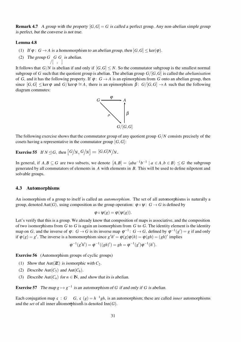
7/26/2019 MATH 2968 Algebra Advanced Notes
http://slidepdf.com/reader/full/math-2968-algebra-advanced-notes 31/110
Remark 4.7 A group with the property [G, G] = G is called a perfect group. Any non-abelian simple group
is perfect, but the converse is not true.
Lemma 4.8
(1) If ϕ : G → A is a homomorphism to an abelian group, then [G, G] ≤ ker(ϕ ).
(2) The group G/[
G,
G] is abelian.
It follows that G/ N is abelian if and only if [G, G] ≤ N . So the commutator subgroup is the smallest normal
subgroup of G such that the quotient group is abelian. The abelian group G/[G, G] is called the abelianisation
of G, and it has the following property. If ϕ : G → A is an epimorphism from G onto an abelian group, then
since [G, G] ≤ kerϕ and G/ kerϕ ∼= A, there is an epimorphism β : G/[G, G] → A such that the following
diagram commutes:
Gϕ A
τ
G/[G, G]
β
The following exercise shows that the commutator group of any quotient group G/ N consists precisely of the
cosets having a representative in the commutator group [G, G]:
Exercise 55 If N G, then [G/ N , G/ N ] = [G,G] N / N .
In general, if A, B ⊆ G are two subsets, we denote [ A, B] = aba−1b−1 | a ∈ A, b ∈ B ≤ G the subgroup
generated by all commutators of elements in A with elements in B. This will be used to define nilpotent and
solvable groups.
4.3 Automorphisms
An isomorphism of a group to itself is called an automorphism. The set of all automorphisms is naturally a
group, denoted Aut(G), using composition as the group operation: ϕ ψ : G → G is defined by
ϕ ψ (g) = ϕ (ψ (g)).
Let’s verify that this is a group. We already know that composition of maps is associative, and the composition
of two isomorphisms from G to G is again an isomorphism from G to G. The identity element is the identity
map on G, and the inverse of ϕ : G → G is its inverse map ϕ −1 : G → G, defined by ϕ −1(g) = g if and only
if ϕ (g) = g. The inverse is a homomorphism since g h = ϕ (g)ϕ (h) = ϕ (gh) = (gh) implies
ϕ −1(gh) = ϕ −1((gh)) = gh = ϕ −1(g)ϕ −1(h).
Exercise 56 (Automorphism groups of cyclic groups)
(1) Show that Aut(ZZ) is isomorphic with C 2.
(2) Describe Aut(C 5) and Aut(C 6).
(3) Describe Aut(C n) for n ∈ IN, and show that its is abelian.
Exercise 57 The map g → g−1 is an automorphism of G if and only if G is abelian.
Each conjugation map ch
: G→
G, ch
(g) = h−
1gh, is an automorphism; these are called inner automorphisms
and the set of all inner automorphisms is denoted Inn(G).
31
7/26/2019 MATH 2968 Algebra Advanced Notes
http://slidepdf.com/reader/full/math-2968-algebra-advanced-notes 32/110
Lemma 4.9 Inn(G)Aut (G).
Lemma 4.10 The map G → Aut(G) defined by g → cg−1 is a homomorphism with image Inn(G) and kernel
Z (G). We therefore have G/ Z (G) ∼= Inn(G).
Remark 4.11 The map G → Aut(G) defined by g → cg is not a homomorphism since it reverses the or-der of multiplication. In general, a map ϕ : G → H is called an anti-homomorphism if for all a, b ∈ G, we
have ϕ (ab) = ϕ (b)ϕ (a). The map g → g−1 is also an anti-homomorphism, and the composition of two anti-
homomorphisms is a homomorphism.
Example 4.12 The map GL(n, F ) → GL(n, F ) defined by A → transpose ( A)−1 is an automorphism. Both
transposition and inversion are anti-automorphisms and they commute; i.e. transpose ( A)−1 = transpose ( A−1).
The quotient group Out(G) = Aut(G)/Inn(G) is the group of outer automorphisms of G.
A normal subgroup is invariant under all inner automorphisms; i.e. if N G and ϕ : G→
G is an inner auto-
morphism, then ϕ ( N ) = N . If the subgroup H ≤ G is invariant under all automorphisms of G, then it is called
characteristic, and we write H char G. The subgroups e and G are always characteristic. Every characteristic
subgroup is normal since it is invariant under all inner automorphisms; the converse is not true:
Example 4.13 In the group Q8, each of the cyclic subgroups of order 4 is normal, but none of these are
characteristic. However, the subgroup 1,−1 is characteristic, since it is the only subgroup of order 2.
Some groups do not have interesting characteristic subgroups:
Exercise 58 Every subgroup of the Klein four group K 4 is normal since this group is abelian. Determine the automorphism group of K 4 and show that the three subgroups of order two are not characteristic.
Lemma 4.14 The commutator subgroup and the centre of a group are characteristic.
Remark 4.15 In order to show that H char G, it suffices to show that α ( H ) ⊆ H for all α ∈ Aut(G). Since if
α ( H ) ⊆ H and α −1( H ) ⊆ H , then for every h ∈ H , we have α −1(h) ∈ H , and hence α (α −1(h)) = h, giving
α ( H ) = H .
As discovered in Exercise 52, the subgroup
1,
−1
of Q8 is its commutator subgroup . So the above lemma
gives another proof of the fact that is characteristic. The lemma also implies that if a group is non-abelian and
not perfect, then it contains at least one interesting characteristic subgroup (since its commutator subgroup is a
non-trivial, proper subgroup).
The following lemma shows that the property characteristic is somewhat stronger than the property normal:
Lemma 4.16 Let A and B be subgroups of the group G.
(1) If A char G and B char G, then A ∩ B char G and AB char G.
(2) A char BG implies AG.
(3) A char B char G implies A char G.
32
7/26/2019 MATH 2968 Algebra Advanced Notes
http://slidepdf.com/reader/full/math-2968-algebra-advanced-notes 33/110
4.4 Exact sequences*
This subsection introduces some useful notation for relationships between groups or properties of homomor-
phisms.
Definition 4.17 (Exact sequence) An exact sequence of groups is a sequence (possibly terminating in either
direction) of the form . . .
ϕ k −2−−→ Gk −1ϕ k −1−−→ Gk
ϕ k −→ Gk +1ϕ k +1−−→ . . . ,
where each ϕ k : Gk → Gk +1 is a homomorphism such that im(ϕ k −1) = ker(ϕ k ) for each k ∈ ZZ.
If an arrow is not labelled, then the homomorphism is a natural one that arises from context; e.g. if H ≤ G, then
H → G is the inclusion map h → h. The trivial group is usually denoted 1 or 0 in such a sequence (depending
on the natural notation for the identity in its image or target group), and there are unique homomorphisms
1 → G and G → 1.
Example 4.18 If ϕ : G → H is a homomorphism, then the following sequence is exact:
1 −→ ker(ϕ ) −→ G −→ im(ϕ ) → 1.
Example 4.19 If N G, then the following sequence is exact:
1 −→ N −→ G −→ G/ N → 1.
Example 4.20 Let ϕ : G → H be a homomorphism. Then ϕ : G → H is
(1) a monomorphism if and only if the sequence 1 −→ G ϕ −→ H is exact.
(2) an epimorphism if and only if the sequence G ϕ −→ H −→ 1 is exact.
(3) an isomorphism if and only if the sequence 1 −→ G ϕ −→ H −→ 1 is exact.
Example 4.21 If ϕ : G → H is a homomorphism, then the first isomorphism theorem states that
1 −→ G/ ker(ϕ ) β −→ im(ϕ ) → 1
is exact, where β is the map from the theorem.
Example 4.22 There is an exact sequence:
1 −→ Z (G) −→ G −→ Aut (G) → Out (G) → 1.
It is no accident that the above sequences do not continue once we encounter the trivial group. Notice that
1
→ G
→ 1 in an exact sequence implies G
∼= 1. Further, . . .
→ G
→ 1
→ 1
→ H
→ . . . gives the same
information as . . . → G → 1 → H → . . . , which gives the same information as when one splits the sequence
into two: . . . → G → 1 and 1 → H → . . . .
4.5 Direct products
Definition 4.23 (Direct product) Given groups G and H , the direct product G × H is defined as follows: The
underlying set of G × H is the cartesian product of G and H , i.e. the set of all ordered pairs
(g, h) | g ∈ G, h ∈ H ,
and the group operation is defined componentwise:
(g1, h1) (g2, h2) = (g1 G g2, h1 H h2).
33
7/26/2019 MATH 2968 Algebra Advanced Notes
http://slidepdf.com/reader/full/math-2968-algebra-advanced-notes 34/110
It is straight forward to check that this defines a group:
(1) It is non-empty since both G and H are.
(2) The group operation is well-defined since the operations in G and H are.
(3) The associative law holds since it holds in both G and H .
(4) The identity element is (eG, e H ).
(5) The inverse of (g, h) is (g−1, h−1).
Notice that neither G nor H are subgroups of G × H , but the maps
G → G × H , g → (g, e H )
and
H → G × H , h → (eG, h)
are monomorphisms with images G × e H and eG × H respectively. As in the previous subsection, the
trivial group will also be denoted 1, so these subgroups are G × 1 and 1 × H .
Exercise 59 Show that the direct product has the following properties:
(1) G × 1G × H and 1× H G × H .
(2) The elements (g, e H ) and (eG, h) commute for all g ∈ G and h ∈ H .
(3) (G × 1) ∩ (1× H ) = 1 × 1
(4) (G × 1) (1 × H ) = G × H
(5) G× H is abelian if and only if both G and H are abelian. In this case, if additive notation is used for the
operation in both G and H , the direct product is also written as G ⊕ H .
Example 4.24 The Klein four group is isomorphic to a direct product: C 2 × C 2 ∼= K 4. To see this, write
C 2 =
g
for the factor on the left and C 2 =
h
for the factor on the right. Then
g
×h
is a group of order 4,
with set of elements (e, e), (e, h), (g, e), (g, h). it is easy to see that every non-trivial element has order two.Whence g×h ∼= K 4.
Example 4.25 We have C 2 ×C 3 ∼= C 6. To see this, write C 2 = g for the factor on the left and C 3 = h for
the factor on the right. Then g×h is a group of order 6. Computing the powers of (g, h) gives:
(g, h)1 = (e, e)
(g, h)2 = (g2, h2) = (e, h2) = (e, e)
(g, h)3 = (g3, h3) = (g, e) = (e, e),
and this implies that (g, h) has order 6, since neither 4 nor 5 divides 6. So C 2 ×C 3 = (g, h) ∼= C 6.
Many groups have the structure of a direct product even though elements are not written as pairs. The following
proposition shows how to identity the structure:
Proposition 4.26 The group K is isomorphic to G × H if and only if there are subgroups G1, H 1 ≤ K such
that:
(1) G1 ∼= G, H 1 ∼= H ;
(2) G1 ∩ H 1 = eK ;
(3) for each k ∈ K there are g ∈ G1 and h ∈ H 1 such that k = gh ;
(4) every element of G1 commutes with every element of H 1.
If K ∼= G × H as above, we also write K = G1 × H 1. This is sometimes called an internal direct product.
34
7/26/2019 MATH 2968 Algebra Advanced Notes
http://slidepdf.com/reader/full/math-2968-algebra-advanced-notes 35/110
Example 4.27 K 4 = (12)(34)×(13)(24) = (12)(34)×(14)(23) = (13)(24)×(14)(23).
Similarly, given the groups G1, . . . , Gn the direct product G1 × . . . × Gn is the cartesian product of the groups
with componentwise multiplication:
(g1, . . . , gn) (h1, . . . , hn) = (g1 G1 h1, . . . , gn Gn
hn).
Moreover, conditions similar to the above exercise can be given to determine whether a group is the directproduct of a finite set of normal subgroups.
Example 4.28
ZZn ∼= ZZ × . . .× ZZ n times
∼= ZZ ⊕ . . .⊕ ZZ n times
,
where the notation ⊕ is used because the operation in ZZ is written as addition.
The direct product of groups is associative and commutative (up to isomorphism) and we can forget the brackets
altogether (again up to isomorphism). For example:
( B×
A)×
C
∼= ( A
× B)
×C
∼= A
×( B
×C )
∼= A
× B
×C .
Exercise 60 Show that C 8, C 4 ×C 2 and C 2 ×C 2 ×C 2 are non-isomorphic abelian groups of order 8.
Exercise 61 The centre of a direct product is the direct product of the centres of the factors.
Exercise 62 The commutator subgroup of a direct product is the direct product of the commutator subgroups
of the factors.
It turns out that the direct product is enough to completely understand the structure of the finite abelian groups
and, more generally, the finitely generated abelian groups.
4.6 Semi-direct products
Definition 4.29 (Semi-direct product) Given the groups N and H and a homomorphism ρ : H → Aut ( N ),
the semi-direct product of N and H (via ρ ) is defined as follows. The underlying set is again N × H , but the
group operation is given by:
(n1, h1) (n2, h2) = (n1 N ρh1(n2), h1 H h2),
where we write h → ρh. This is denoted N ρ H or N H if ρ is understood.
Example 4.30 Let N ∼= C 3 and H ∼= C 2. Write N = e N , x, x2 and H = e H , y. Define ρ : H → Aut(C 3) by
e H → (g → g) and b → (g → g−1
). So ρe H : N → N is the identity map and ρ y : N → N is the inversion map.Then
G = (e N , e H ), ( x, e H ), ( x2, e H ), (e N , y), ( x, y), ( x2, y)is a group of order 6. So either G is cyclic or dihedral. Since
( x, y) ( x2, y) = ( x ρ y( x2), y y) = ( x x, e H ) = ( x2, e H )
and
( x2, y) ( x, y) = ( x2 ρ y( x), y y) = ( x2 x2, e H ) = ( x, e H )
it follows that the multiplication is not commutative and hence G = N ρ H ∼= D3 ∼= Σ3.
The above example shows that, unlike with direct products, the semi-direct product of two abelian groups may
not be abelian. Some key properties of the semi-direct product are summarised in the following exercise.
35
7/26/2019 MATH 2968 Algebra Advanced Notes
http://slidepdf.com/reader/full/math-2968-algebra-advanced-notes 36/110
Exercise 63
(1) Determine the inverse of (n, h) ∈ N ρ H .
(2) The natural inclusion maps ι N : N → N ρ H and ι H : H → N ρ H defined by n → (n, e H ) and h →(eG, h) respectively are monomorphisms.
(3) The image of N under the inclusion map is normal in N H (this is one way to remember the notation);
(4) We have ( N H )/ι N ( N ) ∼= H , so in the language of Section 4.4 there is an exact sequence
1 → N → N H → H → 1.
Here is a method to recognise the structure of a semi-direct product:
Proposition 4.31 Suppose G is a group, N G and H ≤ G. Assume that every element g ∈ G has a unique
expression as g = nh with n ∈ N and h ∈ H . Let ρ : H → Aut( N ) be the representation taking h ∈ H to the
map n → hnh−1. This is well-defined since N is normal. Then G ∼= N ρ H , where the isomorphism is given
by nh → (n, h).
Example 4.32 Using the above exercise, it can be shown that the dihedral group Dn is isomorphic withC nρC 2, where the homomorphism ρ : C 2 → Aut (C n) takes the generator of C 2 to the automorphism g → g−1.
We know that Dn = e, a, a2, . . . , an−1, b, ab, a2b, . . . , an−1b by taking the right cosets of the cyclic group gen-
erated by a rotation a, where b is any of the reflections. We have N = a Dn since its index is two, and we
write H = b. Then every element has a unique expression as g = nh with n ∈ N and h ∈ H . This shows that
Dn ∼= N ρ H , where ρh(n) = hnh−1. Now ρb(ak ) = bak b−1 = bak b. To bring this expression into the form
(power of a) × (power of b), we move the leftmost b to the right of ak using the relation ba = a−1b:
ρb(ak ) = bak b−1 = bak b = a−k b2 = a−k .
So ρ is the claimed automorphism.
4.7 Summary
In the previous sections, examples of groups arose from familiar contexts, such as matrix groups, permutation
groups or symmetry groups of geometric objects. We have now seen groups arise at a more abstract level, by
considering the automorphism groups of groups (which can be viewed as the symmetry groups of groups), or
by taking direct or semi-direct products of groups. In this, we have also seen the subtlety involved in building
new groups from old ones even if the building blocks are rather simple.
36
7/26/2019 MATH 2968 Algebra Advanced Notes
http://slidepdf.com/reader/full/math-2968-algebra-advanced-notes 37/110
5 Abelian, nilpotent and solvable groups
The cyclic groups have been classified in §3, and we also completely understand their subgroups. The next
simplest class of groups are the abelian groups, since commutativity gives many nice properties that do not
hold in non-abelian groups in general. For instance, every subgroup is normal and the product of any two
torsion elements is again a torsion element. This section applies the theory developed so far to classify the
finitely generated abelian groups. After this, we briefly look at the class of nilpotent groups (which contains
the abelian groups) and the class of solvable groups (which contains the nilpotent groups).
5.1 The classification problem
In general terms, the classification problem for a set S of mathematical objects (such as groups, simple groups,
Platonic solids, perfect squares, . . . ) asks to determine a complete list of all objects in S (without duplications)
as well as an algorithm which determines for any given object in S , where it is on the list.
One usually faces the problem that one needs to restrict to a class of objects that is large enough to lead to an
interesting classification, but small enough to be able to say something meaningful. For instance, it is known
that there is no algorithm that can, given any groups G and H , determine whether or not G is isomorphic
with H . (In fancy language: the isomorphism problem is undecidable). Hence it is not possible to give a
classification of all groups (and the same is true if one restricts to the class of finitely presented groups).
However, it is possible to classify smaller classes of groups (such as the simple groups or the finitely generated
abelian groups), and these classifications are extremely useful.
5.2 Finite abelian groups
Throughout this subsection, A denotes an abelian group. I’ll start this section with an exercise that gives some
feeling for the structure of finite abelian groups:
Exercise 64 Suppose A is finite, and | A| =k
∏ j=1
pn j
j is the prime factorisation of the order of A. Then the length
of any composition series of A isk
∑ j=1
n j. Hint: Talk to Jordan and H¨ older.
The abelian group A has the following wonderful property:
(gh)n = gnhn
for all g, h
∈ A and n
∈ZZ. It follows that
A(n) = g ∈ A | gn = eis a (normal) subgroup of A for each n ∈ IN.
Example 5.1 C 4(4) = C 4, C 4(2) ∼= C 2; K 4(4) = K 4 = K 4(2); K 4(3) = 1.
Lemma 5.2 Suppose A is a finite abelian group and A = A(n). Then the order of A is a number all of whose
prime factors are prime factors of n.
Example 5.3 Let A = C 2 ×C 2 ×C 3 ×C 6 and n = 6. Then A = A(6) and | A| = 23 · 32.
Positive integers m and n with gcd(m, n) = 1 are said to be coprime.
37
7/26/2019 MATH 2968 Algebra Advanced Notes
http://slidepdf.com/reader/full/math-2968-algebra-advanced-notes 38/110
Lemma 5.4 If gcd(m, n) = 1, then A(mn) = A(m)× A(n).Moreover, if | A| = mn, then | A(m)| = m and | A(n)| = n.
Example 5.5 Letting C 6 = g gives C 6(2) = g3 and C 6(3) = g2. Whence C 6(6) = C 6(2) ×C 6(3). This
is just an internal version of C 6 ∼= C 2 ×C 3.
Theorem 5.6 (Rough decomposition of finite abelian groups) Suppose A is finite and | A| =k
∏ j=1
pn j
j is the
prime factorisation of the order of A. Then A is the direct product
A ∼= A( pn1
1 )× . . . × A( pnk
k ),
and | A( pn j
j )| = pn j
j for each j ∈ 1, . . . k .
The above theorem cannot be the desired classification as demonstrated by the Klein four group:
K 4 = K 4(22) = K 4(2) ∼= C 2 ×C 2,
whilst C 4 = C 4(22) > C 4(2) ∼= C 2. The missing step is to analyse how the groups A( pn j
j ) in Theorem 5.6 are
decomposed. For this analysis, it suffices to assume that an abelian group A is given with | A| = pn
, where p isa prime number. Then A = A( pn) since every element raised to the order of a group is the identity.
Proposition 5.7 (Recognising the structure of the factors) Suppose A is an abelian group with | A| = pn,where p is a prime number.
(1) A is cyclic if and only if it contains a unique subgroup of order p.
(2) If a ∈ A is an element of maximal order in A, then there is a subgroup B ≤ A such that A = a× B.
(3) A is a direct product of cyclic groups. Moreover, if
A ∼= g1× . . .×gk ∼= h1× . . .×hm,
then k = m and, after possibly renumbering the elements, one has o(h j) = o(g j).
Corollary 5.8 (Structure of finite cyclic groups) Suppose A is finite and | A| =k
∏ j=1
pn j
j is the prime factorisa-
tion of the order of A. Then A is cyclic if and only if each A( pn j
j ) is cyclic.
Theorem 5.6 and Proposition 5.7 give the desired classification of the finite abelian groups, since they provide
us with both a list of all isomorphism classes of finite abelian groups, as well as an algorithm to recognise
where in this list a given finite abelian group is. The list is, of course, infinite, and best organised by order and
then by partitions of the exponents in the prime factorisation of the order; here is a sample entry of the list:
Example 5.9 Suppose A is abelian and | A| = 1000 = 23 53. Then A is isomorphic to exactly one of the following nine groups:
C 2 ×C 2 ×C 2 ×C 5 ×C 5 ×C 5
C 2 ×C 2 ×C 2 ×C 5 ×C 52
C 2 ×C 2 ×C 2 ×C 53
C 2 ×C 22 ×C 5 ×C 5 ×C 5
C 2 ×C 22 ×C 5 ×C 52
C 2 ×C 22 ×C 53
C 23
×C 5
×C 5
×C 5
C 23 ×C 5 ×C 52
38
7/26/2019 MATH 2968 Algebra Advanced Notes
http://slidepdf.com/reader/full/math-2968-algebra-advanced-notes 39/110
C 23 ×C 53
Only the last group in this list is cyclic; each of the remaining groups can be generated with 2 or 3 elements.
Example 5.10 The group C 10 ×C 20 ×C 5 is abelian and has order 10 · 20 · 5 = 1000, and hence is isomorphic
to a group in the above list. We have C 10 ∼= C 2 ×C 5 and since C 20 is cyclic, we have C 20
∼= C 22 ×C 5. Whence
C 10 ×C 20 ×C 5 ∼= C 2 ×C 22 ×C 5 ×C 5 ×C 5.
Exercise 65 K 4 ×C 250 ∼= C 2 ×C 2 ×C 2 ×C 53
Exercise 66 Every abelian group of order 2310 is cyclic.
Exercise 67 Determine the number of isomorphism classes of abelian groups of the following orders: 2000,
3000, 5000, 7000, 11000.
5.3 Finitely generated abelian groups*
The classification of the finitely generated abelian groups is easy to state with the material covered so far (and is
hence included here), but its proof would require the developments of some more ideas (which will be omitted
for the time being).
It follows from Exercise 11 and the fact that o(g) = o(g−1) that the set of all torsion elements of an arbitrary
abelian group A is a subgroup of A. Denote this subgroup tor( A); it is normal in A since A is abelian.
Lemma 5.11 Suppose A is a finitely generated abelian group. Then tor( A) is a finite group.
Theorem 5.12 Let A be a finitely generated abelian group. Then A/ tor( A) ∼= ZZn for some uniquely deter-
mined n ∈ IN ∪0, and A ∼= ZZn × tor( A).
5.4 Nilpotent groups*
Definition 5.13 (Nilpotent) Define G1 = [G, G], G2 = [G, G1] and inductively Gk +1 = [G, Gk ], giving a chain
of subgroups
G = G0 ≥ [G, G] ≥ [G, G1] ≥ . . . ≥ [G, Gn] ≥ . . .
Then G is nilpotent if Gk +1 is trivial for some k . The number of non-trivial groups in the chain is then called
the nilpotency class of G.
Example 5.14 The trivial group is the only nilpotent group of nilpotency class 0. Every non-trivial abelian
group is nilpotent of nilpotency class 1.
Exercise 68 Show that Q8 is nilpotent. What is its nilpotency class?
If a finite group is not nilpotent, then the chain of subgroups must stabilise at a non-trivial subgroup. For
instance, taking the symmetric group G = Σn with n ≥ 3, we obtain G1 = [Σn,Σn] = A n, and hence
G2 = [G, G1] = [Σn,A n].
I claim that [Σn,A n] = A n. This can be argued quickly for n ≥ 4 since [Σn,A n] ≥ [A n,A n] = A n. However,
this proof breaks down for the small cases since [A 4,A 4] = K 4 and [A 3,A 3] = 1. In general, it suffices to show
that [Σn,A n] contains every 3–cycle since A n is generated by the 3–cycles. This is shown with the following
calculation:
[(ab), (abc)] = (ab)(abc)(ab)(cba) = (bac)(cba) = (abc).
39
7/26/2019 MATH 2968 Algebra Advanced Notes
http://slidepdf.com/reader/full/math-2968-algebra-advanced-notes 40/110
Hence we have:
A n = G1 ≥ G2 = [G, G1] = [Σn,A n] = A n,
which forces G2 = A n and so Gk = [Σn,A n] = A n for each k ≥ 1. In particular Σ3, the smallest non-abelian
group, is not nilpotent.
Here is a family of groups that shows that the nilpotency class can be arbitrarily large:
Example 5.15 The dihedral group D2n is nilpotent of class n for n ≥ 1.
Exercise 69 Suppose G is nilpotent. Then every Gk is normal in G and every quotient G/Gk is nilpotent.
The chain G = G0 ≥ [G, G] ≥ [G, G1] ≥ . . . ≥ [G, Gn] = 1 is therefore a normal series, and called the lower
central series for G. Its length is the nilpotency class of G.
The nilpotency class gives a way of measuring how far from being abelian a nilpotent group is. Every subgroup
and every quotient group of a nilpotent group G of class n is nilpotent and of class at most n. Groups of class
2 are still pretty close; for instance:
Exercise 70 Suppose G is a nilpotent group of class 2. Show that for all g, h ∈ G, we have:
(gh)n = gnhn[h, g]n(n−1)/2.
Hint: use induction on n.
Exercise 71 Define Nil to be the subgroup of SL(3, IR) consisting of all matrices of the form 1 x z
0 1 y
0 0 1
,
where x, y, z ∈ IR. This is usually called the Heisenberg group. Verify that Nil is nilpotent and non-abelian.
There is a bijection Nil → IR3 given by 1 x z
0 1 y
0 0 1
→ ( x, y, z).
This can be made into an isomorphism by giving IR 3 the following group operation:
( x, y, z) ( x, y, z) = ( x + x, y + y, z + z + xy).
It is customary to work with matrices instead of (IR3,). Composing this map with the projection onto the first
two coordinates gives an epimorphism ρ : Nil → (IR2, +). There also is a monomorphism σ : (IR, +) → Nilgiven by
z →1 0 z
0 1 0
0 0 1
.
Exercise 72 Show that the sequence
0 −→ IR σ −→ Nil
ρ−→ IR2 → 0
is exact.
Lemma 5.16 Subgroups and homomorphic images of nilpotent groups are nilpotent.
40
7/26/2019 MATH 2968 Algebra Advanced Notes
http://slidepdf.com/reader/full/math-2968-algebra-advanced-notes 41/110
5.5 Solvable groups*
Definition 5.17 (Solvable) Let G0 = [G, G] and define Gk = [Gk −1, Gk −1] for each k ∈ IN. Since the com-
mutator subgroup is normal, this gives a normal series, called the derived series:
G ≥ G0 ≥ G1 ≥ . . . ≥ Gn ≥ . . .
If Gk is trivial for some k
∈IN, then G is solvable, and the number of non-trivial groups in the above series is
the derived length of G.
Exercise 73 Every nilpotent group is solvable.
Lemma 5.18 Subgroups and homomorphic images of solvable groups are solvable.
The above lemma has a striking converse:
Proposition 5.19 Suppose G is a group and ING has the property that both N and G/ N are solvable. Then
G is also solvable.
Example 5.20 The dihedral group Dn is solvable. This follows since Dn the subgroup generated by a rotation
is solvable since it is cyclic and normal since it has index two. The quotient group is also solvable since it iscyclic, and so Dn is solvable.
Remark 5.21 The above example also shows that a result analogous to Proposition 5.19 cannot hold for
nilpotent groups, since Σ3 = D3 is not nilpotent.
Notice that if a group G is solvable and has a composition series, then any composition series for G will only
have abelian factors. Moreover, if G is finite then by the classification of abelian groups, any composition
series will only have factors that are cyclic of prime order. This gives a quick way to see that the symmetric
groups Σn for n ≥ 5 are not solvable. We had previously shown that the symmetric groups Σn for n ≥ 3 are
not nilpotent.
Example 5.22 The groups Σ3 and Σ4 are solvable since
Σ3 ≥ [Σ3,Σ3] =A 3 ≥ [A 3,A 3] = 1,
and
Σ4 ≥ [Σ4,Σ4] = A 4 ≥ [A 4,A 4] = K 4 ≥ [K 4, K 4] = 1.
Proposition 5.23 The group G is a finite solvable group if and only if is has a composition series with all
factors cyclic of prime order.
Notice that if a finite group is not solvable, then the above normal series must stabilise at a group which satisfies
G = [G, G]. This is called a perfect group. The smallest perfect group is A 5 (and this is also the smallest non-
abelian simple group). So all finite groups of order less than 60 are solvable.
Exercise 74 If G is solvable, then every Gk is normal in G and every quotient G/Gk is solvable.
Similar to the Heisenberg group Nil, there is a “3–dimensional” solvable group Sol obtained by giving IR 3 a
fancy group operation:
( x, y, z) ( x, y, z) = ( x + e− z x, y + e z y, z + z).
This has the structure of a semi-direct product IR IR2, where the homomorphism IR → Aut(IR2) takes t ∈ IR
to the map ( x, y) → (et x, e−t y). Hence there is a short exact sequence
0 −→ IR2 −→ Sol −→ IR → 0.
Remark 5.24 The celebrated Feit-Thompson theorem (whose original proof occupies a mere 255 pages) states
that every finite group of odd order is solvable.
41
7/26/2019 MATH 2968 Algebra Advanced Notes
http://slidepdf.com/reader/full/math-2968-algebra-advanced-notes 42/110
6 Group actions
The study of group actions is now taken further, and different actions of a group on itself, in particular left-
multiplication and conjugation, are used to obtain fundamental results about the structure of finite groups.
6.1 Symmetry groups
The group of symmetries of a regular n–gon is isomorphic with a subgroup of Σn. This fact has a vast gener-
alisation, which reduces the study of all groups to the study of the subgroups of permutation groups. Recall
that the symmetric group consists of all permutations of a set, ignoring any additional structure that the set may
have.
Theorem 6.1 (Cayley) A group G is isomorphic with a subgroup of the symmetric group on G .
A candidate map from G to Sym(G) is given by h → lh, where lh : G → G defined by lh(g) = hg. This is
well-defined since left-multiplication is a bijection. It remains to show that it is indeed a homomorphism and
injective:
Exercise 75 Check that the map G → Sym(G) taking h → lh is a monomorphism.
For a mathematical object X , we also defined the symmetry group of all permutations in Sym ( X ) that pre-
serve the extra (usually implicit) structure. For a group G, this is the automorphism group Aut(G) which
preserves the group structure. For example, the symmetric group Sym(ZZ) is an infinite permutation group,
whilst Aut(ZZ) is isomorphic with C 2.
6.2 Stiffenings
Definition 6.2 (Stiffening) If G is the group of symmetries of some mathematical object X , such as the group of isometries of a metric space or the symmetry group of a triangle, and H ≤ G, then H corresponds to
the group of symmetries of a more rigid structure on X . This is called a stiffening of (G, X ).
For instance, if all edges of an equilateral triangle are oriented then not all symmetries of the triangle-without-
edge-orientations will preserve the orientations.
Exercise 76 Determine all possible stiffenings arising from orienting the edges of an equilateral triangle.
6.3 Orbit and stabiliser
Using the notion of a homomorphism, we can restate the definition of group action as follows; you should
check that the two definitions are indeed equivalent.
Definition 6.3 (Group action) An action of a group G on a mathematical object X is a group homomorphism
G → Sym( X ).
Given a group action G X , the homomorphism G → Sym( X ) is a representation of G. The representation
is faithful if the representation is a monomorphism, i.e. if for every e = g ∈ G there is x ∈ X such that g · x = x.In this case, the action of G on X is called effective.
For instance, the dihedral group Dn permutes the vertices of the regular n–gon, giving a representation Dn →Σ
n. Since every non-trivial element moves some vertex, the representation is faithful. More generally, Theo-
rem 6.1 states that every group can be faithfully represented as a group of permutations.
42
7/26/2019 MATH 2968 Algebra Advanced Notes
http://slidepdf.com/reader/full/math-2968-algebra-advanced-notes 43/110
Definition 6.4 (Orbit) The orbit of x ∈ X under G X is G · x = g · x | g ∈ G ⊆ X .
Definition 6.5 (Stabiliser) The stabiliser of x ∈ X under G X is G x = StabG( x) = g ∈ G | g · x = x ⊆ G.
Exercise 77 Suppose G X .
(1) The stabiliser of x
∈ X is a subgroup of G.
(2) Every element of X lies in one and only one orbit. Whence the orbits partition X .
Examples 6.6
(1) The group SO(2, IR) acts on IR2. The orbit of any point is the circle centred at the origin passing through
the point. (This includes a circle of radius 0, consisting just of the origin.) The stabiliser of the origin is
the whole group, the stabiliser of any other point is the trivial group.
(2) The group SO(3, IR) acts on IR3. The orbit of any point is the sphere centred at the origin passing through
the point. (This includes a sphere of radius 0, consisting just of the origin.) The stabiliser of the origin
is the whole group. The stabiliser of any other point consists of all rotations whose axis passes through
this point and the origin.
The Orbit-Stabiliser Relation 6.7 Suppose G X . Then for each x ∈ X there is a bijective correspondence
between the left cosets of the stabiliser G x and the elements of the orbit G · x. Hence the index of G x in G
equals the size of G · x (possibly infinite),
|G : G x| = |G · x|.In particular, if G is finite, then
|G| = |G x| · |G · x|,and so |G · x| divides |G|.
6.4 Conjugation
We have already used the action of a group on itself by left multiplication to deduce Cayley’s theorem. Another
important action of a group on itself is conjugation:
g · h = ghg−1
for all g, h ∈ G. In this case, orbit and stabiliser have special names:
Definition 6.8 (Conjugacy class and centraliser) Let G X by conjugation. The orbit of h ∈ G is called the
conjugacy class of h, and the stabiliser of h ∈ G is called its centraliser. We write ccl(h) = cclG(h) = G ·h and
C (h) = C G(h) = Gh.
Note that each g ∈ C G(h) = Gh satisfies h = ghg−1, which is equivalent to gh = hg. Hence C G(h) is the
subgroup of all elements of G that commute with h,
C G(h) = g ∈ G | gh = hg ≤ G.
I’ll also write the conjugacy class in set notation:
cclG(h) = ghg−1 | g ∈ G ⊆ G.
Let G be a group. Conjugation defines an equivalence relation on G : g ∼ h if and only if there is k ∈ G
such that h = kgk −1. The equivalence classes are the conjugacy classes, and the set of all elements whose
equivalence classes contain a single element is precisely the centre of G. This gives the following important
equation:
43
7/26/2019 MATH 2968 Algebra Advanced Notes
http://slidepdf.com/reader/full/math-2968-algebra-advanced-notes 44/110
Class Equation 6.9 Let C 1, . . . ,C n be the conjugacy classes of elements in the finite group G, which contain
more than one element, and let ck ∈C k . Then |C k | = |G : C G(ck )| by the orbit-stabiliser relation, and so:
|G| = | Z (G)|+n
∑k =1
|G : C G(ck )|.
Exercise 78 Let G be a group. Show that every normal subgroup of G is a disjoint union of conjugacy classes.
We will now deduce various applications to group theory arising from the action of a group on itself by conju-
gation, showing how this action leads to information about the abstract structure of a group.
6.5 First applications to group theory
Lemma 6.10 Let p be a prime and let G be a group of order pn for some integer n ≥ 1. Then the centre of G
contains more than one element.
Theorem 6.11 Every group of order p2, where p is a prime, is abelian (and hence isomorphic to C p2 or C p ×C p ).
Definition 6.12 If |G| = pn, where p is a prime, then G is called a p–group.
The above theorem generalises to show that every p–group is nilpotent. Non-abelian groups of order 23 = 8
are D4 and Q8. A non-abelian group of order 33 = 27 is the following semi-direct product of C 9 and C 3 :
C 9C 3 = a, b | a9 = b3 = e, bab−1 = a4.
The following is an extremely useful consequence of the orbit-stabiliser relation:
Example 6.13 (Fixed point congruence for p–groups) Suppose |G| = pn and G X , where X is a finite
set. Write
FixG( X ) = x ∈ X | g · x = x for all g ∈ G.
Then FixG( X ) is the union of all orbits consisting of precisely one elements. Any other orbit G · x, x /∈ FixG( X ),has at least two elements, and by the orbit-stabiliser relation, |G · x| divides |G| = pn. In particular, |G · x| = k p
for some k ≥ 1. Now X is partitioned into orbits of the action, and hence we have
| X | ≡ |FixG( X )| mod p.
6.6 Normaliser
The normaliser of H ≤ G is the set
N G( H ) = g ∈ G | gHg−1 = H .
I claim that H N G( H ) ≤ G. This is clearly true if N G( H ) is a subgroup of G. The latter can either be shown
by a direct computation or by observing that G acts by conjugation on the set of all subsets of G, which is
usually denoted P (G) and called the power set of G. Then N G( H ) is the stabiliser of the element H ∈P (G)under the action, and hence a subgroup.
Note that |G : N G( H )| is the number of distinct conjugates of H in G.
Since H N G( H ), we may form the quotient group N G( H )/ H , and this has the following interpretation.
44
7/26/2019 MATH 2968 Algebra Advanced Notes
http://slidepdf.com/reader/full/math-2968-algebra-advanced-notes 45/110
Example 6.14 Let G be any finite group and H ≤ G be a subgroup. Then H acts on the set of all left-cosets
X = gH | g ∈ G by left-multiplication:
h · gH = hgH .
We have h · H = hH = H for each h ∈ H , and so H is a fixed point in X for the action. Are there any other
fixed points? We have:
h · gH = gH for all h ∈ H ⇐⇒ g−1hgH = H for all h ∈ H
⇐⇒ g−1 Hg ⊆ H
⇐⇒ g−1 Hg = H
⇐⇒ g ∈ N G( H ).
So Fix H ( X ) = gH ∈ X | h · gH = gH = gH | g ∈ N G( H ). Now H N G( H ), and hence
Fix H ( X ) = gH | g ∈ N G( H ) = N G( H )/ H .
6.7 Sylow’s theorems
We are now able to prove the most fundamental results about finite groups.
Cauchy’s Theorem 6.15 Suppose G is a finite group, p a prime number and n ∈ IN. If p divides |G|, then G
contains an element of order p.
An immediate consequence of the above theorem is that the divisors of |G| are important invariants of the finite
group G. The following is a nice application of Cauchy’s theorem:
Exercise 79 If p is an odd prime and G is a group of order 2 p, then G is isomorphic to either the cyclic group
C 2 p or the dihedral group D p.
The three parts of the next theorem are referred to as the three Sylow theorems.
Sylow’s Theorems 6.16 Suppose pm is the highest power of p dividing the order of the finite group G.
(1) For each 1 ≤ n ≤ m, G has a subgroup of order pn. Moreover, each such subgroup is contained in a
subgroup of order pm.
(2) Any two subgroups of order pm are conjugate in G;
i.e. if H , K ≤ G and | H | = pm = |K |, then there is g ∈ G such that gHg−1 = K .
(3) The number of distinct subgroups of G of order pm
(a) is congruent to 1 modulo p , i.e. of the form 1 + kp for k ≥ 0, and
(b) divides |G|
pm .
A maximal p–subgroup of G is called a Sylow p–subgroup or S p –subgroup; maximal means that it is a p–
subgroup of G which is not contained in any other p–subgroup of G. Denote
Syl p(G) = H ≤ G | H is a S p –subgroup of G.
Note that Syl p(G) only contains the trivial group if p does not divide the order of G, and it only contains G if
G is a p–group. One can paraphrase Sylow’s theorems in this language; for instance the third Sylow theorem
states:
|Syl p(G)| ≡ 1 mod p and |Syl p(G)| divides |G| pm
.
Each of the above theorems can be proved using an action of a group on a set. The different settings are
summarised in below table, and the reader is encouraged to construct proofs using this information.
45
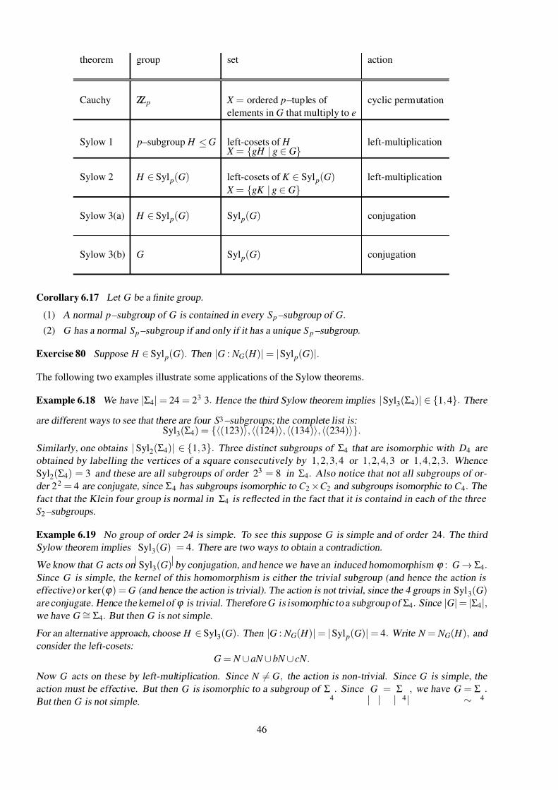
7/26/2019 MATH 2968 Algebra Advanced Notes
http://slidepdf.com/reader/full/math-2968-algebra-advanced-notes 46/110
theorem group set action
Cauchy ZZ p X = ordered p–tuples of cyclic permutation
elements in G that multiply to e
Sylow 1 p–subgroup H ≤ G left-cosets of H left-multiplication X = gH | g ∈ G
Sylow 2 H ∈ Syl p(G) left-cosets of K ∈ Syl p(G) left-multiplication
X = gK | g ∈ G
Sylow 3(a) H ∈ Syl p(G) Syl p(G) conjugation
Sylow 3(b) G Syl p(G) conjugation
Corollary 6.17 Let G be a finite group.
(1) A normal p–subgroup of G is contained in every S p –subgroup of G.
(2) G has a normal S p –subgroup if and only if it has a unique S p –subgroup.
Exercise 80 Suppose H ∈ Syl p(G). Then |G : N G( H )| = |Syl p(G)|.
The following two examples illustrate some applications of the Sylow theorems.
Example 6.18 We have |Σ4| = 24 = 23 3. Hence the third Sylow theorem implies |Syl3(Σ4)| ∈ 1, 4. There
are different ways to see that there are four S 3 –subgroups; the complete list is:Syl3(Σ4) = (123),(124),(134), (234).
Similarly, one obtains | Syl2(Σ4)| ∈ 1, 3. Three distinct subgroups of Σ4 that are isomorphic with D4 are
obtained by labelling the vertices of a square consecutively by 1, 2, 3, 4 or 1, 2, 4, 3 or 1, 4, 2, 3. Whence
Syl2(Σ4) = 3 and these are all subgroups of order 23 = 8 in Σ4. Also notice that not all subgroups of or-
der 22 = 4 are conjugate, since Σ4 has subgroups isomorphic to C 2 ×C 2 and subgroups isomorphic to C 4. The
fact that the Klein four group is normal in Σ4 is reflected in the fact that it is containd in each of the three
S 2 –subgroups.
Example 6.19 No group of order 24 is simple. To see this suppose G is simple and of order 24. The third
Sylow theorem implies
|Syl3(G)
|= 4. There are two ways to obtain a contradiction.
We know that G acts on Syl3(G) by conjugation, and hence we have an induced homomorphism ϕ : G → Σ4.Since G is simple, the kernel of this homomorphism is either the trivial subgroup (and hence the action is
effective) or ker(ϕ ) = G (and hence the action is trivial). The action is not trivial, since the 4 groups in Syl3(G)are conjugate. Hence the kernel of ϕ is trivial. Therefore G is isomorphic to a subgroup of Σ4. Since |G| = |Σ4|,we have G ∼= Σ4. But then G is not simple.
For an alternative approach, choose H ∈ Syl3(G). Then |G : N G( H )| = |Syl p(G)| = 4. Write N = N G( H ), and
consider the left-cosets:
G = N ∪ aN ∪ bN ∪ cN .
Now G acts on these by left-multiplication. Since N = G, the action is non-trivial. Since G is simple, the
action must be effective. But then G is isomorphic to a subgroup of Σ4
. Since |
G|
=|Σ
4|, we have G
∼= Σ
4.
But then G is not simple.
46
7/26/2019 MATH 2968 Algebra Advanced Notes
http://slidepdf.com/reader/full/math-2968-algebra-advanced-notes 47/110
Exercise 81 Show that every group of order 15 is cyclic.
Exercise 82 Suppose |G| = pq, where p and q are primes with p > q. Then G has a normal S p –subgroup.
In particular, G is not simple.
Exercise 83 Suppose
|G
|= pqr , where p, q and r are primes with p > q > r . Then G is not simple.
Exercise 84 Show that the order of a non-abelian simple group is at least 60.
We have already shown that A 5 is a non-abelian simple group of order 60.
Theorem 6.20 Every simple group of order 60 is isomorphic to the alternating group A 5.
6.8 The Cayley graph of a finitely generated group*
Let G be a group with the finite generating set S . Form a graph Γ = Γ (G, S ) with the set of vertices
V (Γ ) = G,
and the set of edges
E (Γ ) = (g, gs) | g ∈ G, s ∈ S .
Note that this graph may be infinite, but it is locally finite: there are only finitely many edges incident with any
vertex. The graph is also connected. It is often considered as a directed graph, with g as the initial and gs as
the terminal vertex of (g, gs).
As a geometric object, it is convenient to assume that e /∈ S , S = S −1 and to think of the pair of edges (g, gs)and (gs, g) = ((gs), (gs)s−1) as one undirected edge. We turn Γ into a metric space by giving each edge length
one and measuring distance between points by shortest paths. So V (Γ ) = G inherits a metric called the word
metric. The group G acts on itself by left-multiplication, and this action is an isometry of the word metric.Moreover, it can be extended to an isometric action of G on Γ .
For g ∈ G, the length of the shortest word in the generators representing g is (g) = S (g) = d (1, g). This gives
the convenient identity
d (g, h) = (g−1h).
Changing the set of generators changes the word metric on G and hence the geometry. It turns out that the
metrics (and graphs) obtained for any two generating sets are quasi-isometric (the graphs look the same up to a
constant plus distortion by at most a constant factor).
Example 6.21 For G = ZZ2 = ZZ⊕ZZ, the Cayley graph is the square grid in IR2 with set of vertices the points
with integer coordinates.
The action of a group on a Cayley graph can be viewed again as an action of the group on itself by left-
multiplication, but the topology of the graph gives new information about the group, and allows conceptually
simpler proofs of facts that have complicated algebraic arguments (an example is given in §9.1). This, however,
is material for a different course.
47
7/26/2019 MATH 2968 Algebra Advanced Notes
http://slidepdf.com/reader/full/math-2968-algebra-advanced-notes 48/110
7 Some linear groups over finite fields
The main examples of finite groups so far have been the symmetric and alternating groups, as well as dihedral
groups and other symmetry groups of geometrical objects. The main purpose of this section is to enlarge our
zoo of examples, and to bring in techniques from linear algebra and projective geometry. The title of this
section is somewhat misleading: some results about vector spaces over arbitrary fields or vector spaces over
algebraically closed fields are included.
7.1 Fields
Definition 7.1 A field is a set F with two operations
+ : F × F → F (a, b) → a + b
· : F × F → F (a, b) → a · b
such that (F , +) is an abelian group (with identity denoted 0), and (F \ 0, · ) is an abelian group (with
identity denoted 1), and the distributive law holds:
(a + b) · c = a · c + b · c
for all a, b, c ∈ F .
We call 0 the additive identity of the field F and 1 its multiplicative identity, (F , +) the additive group of F
and (F \0, · ) the multiplicative group and denote the latter F ×. We also write ab = a ·b, a−b = a + (−b),and a
b = ab−1.
Exercise 85 For all a ∈ F , we have 0 · a = 0.
Exercise 86 If ab = 0 with a, b
∈F , then a = 0 or b = 0.
Examples of fields are Q, IR, and C with their usual operations of addition and multiplication. From now on,
we need to take care to say whether we consider each of them as a field or as a group. There is a natural notion
of a subfield F ≤ F , namely a subset F ⊆ F that is a field with respect to the operations of F . So Q ≤ IR ≤ C.A field with at most finitely many elements is termed a finite field .
Example 7.2 Consider the group ZZn = ZZ/nZZ, and write [a]n = a + nZZ. We have the usual addition
[a]n + [b]n = [a + b]n
and we define a multiplication by
[a]n
·[b]n = [ab]n.
We know that the addition is well-defined and it is easy to verify that the multiplication is also well-defined, i.e.
if [c]n = [a]n and [d ]n = [b]n, then [ab]n = [cd ]n. If n = pq is not a prime, then [ p]n = [0]n and [q]n = [0]n but
[ pq]n = [n]n = [0]n, and this multiplication does not make ZZn into a field.
If n is a prime, say n = p, then this does make ZZ p into a field. To check that ZZ p \ [0] p is indeed a group
with respect to the multiplication we note that associativity follows from the associativity of multiplication in
ZZ, and the identity element is [1] p. It remains to show that every element has a multiplicative inverse. This is
left as an exercise. The field with underlying set ZZ p = ZZ/ pZZ and the above operations is denoted IF p.
Exercise 87 Let p be a prime and [a] p ∈ ZZ p \[0] p. Show that there is [b] p ∈ ZZ p such that [a] p · [b] p = [1] p.
We often denote the element [n] p of IF p by n, and perform arithmetic modulo p.
48
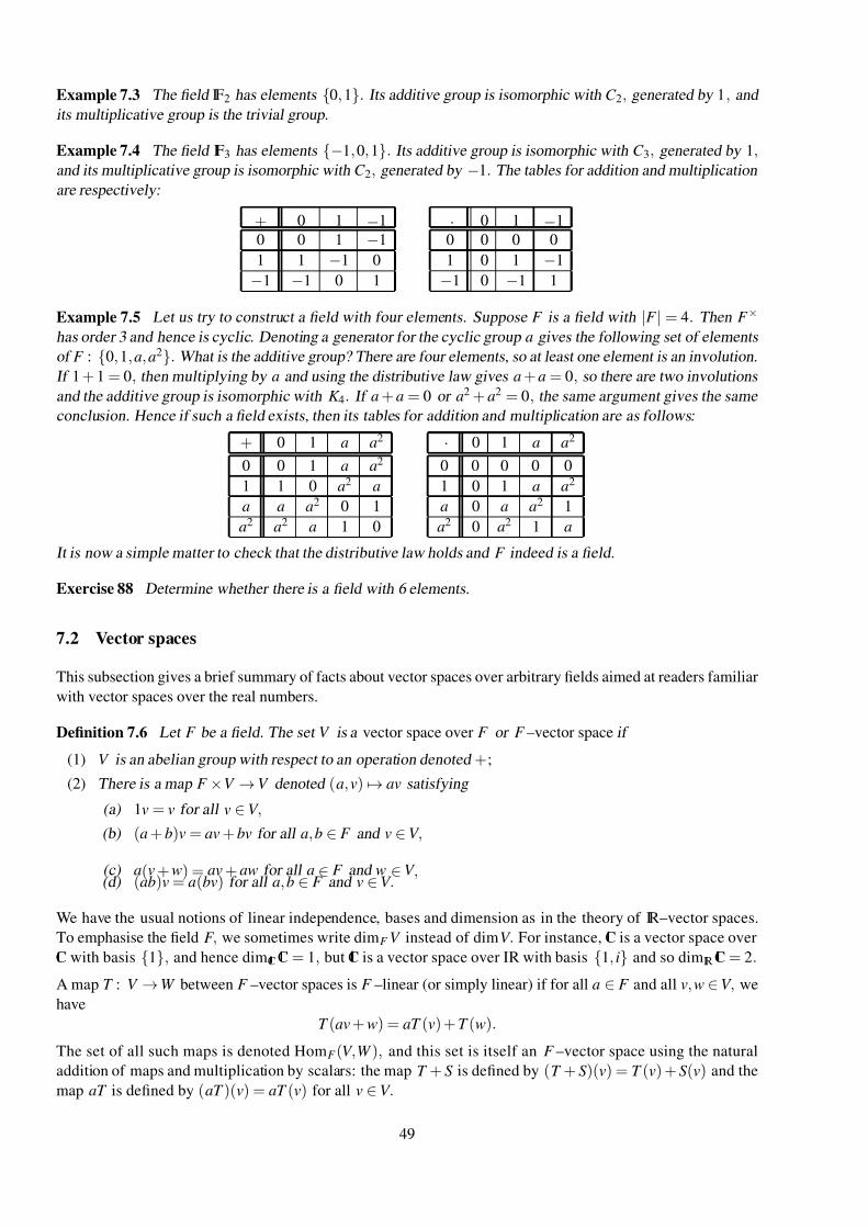
7/26/2019 MATH 2968 Algebra Advanced Notes
http://slidepdf.com/reader/full/math-2968-algebra-advanced-notes 49/110
Example 7.3 The field IF2 has elements 0, 1. Its additive group is isomorphic with C 2, generated by 1, and
its multiplicative group is the trivial group.
Example 7.4 The field IF3 has elements −1, 0, 1. Its additive group is isomorphic with C 3, generated by 1,and its multiplicative group is isomorphic with C 2, generated by −1. The tables for addition and multiplication
are respectively:
+ 0 1 −1
0 0 1 −1
1 1 −1 0
−1 −1 0 1
· 0 1 −1
0 0 0 0
1 0 1 −1
−1 0 −1 1
Example 7.5 Let us try to construct a field with four elements. Suppose F is a field with |F | = 4. Then F ×
has order 3 and hence is cyclic. Denoting a generator for the cyclic group a gives the following set of elements
of F : 0, 1, a, a2. What is the additive group? There are four elements, so at least one element is an involution.
If 1 + 1 = 0, then multiplying by a and using the distributive law gives a + a = 0, so there are two involutions
and the additive group is isomorphic with K 4. If a + a = 0 or a2 + a2 = 0, the same argument gives the same
conclusion. Hence if such a field exists, then its tables for addition and multiplication are as follows:
+ 0 1 a a2
0 0 1 a a2
1 1 0 a2 a
a a a2 0 1
a2 a2 a 1 0
· 0 1 a a2
0 0 0 0 0
1 0 1 a a2
a 0 a a2 1
a2 0 a2 1 a
It is now a simple matter to check that the distributive law holds and F indeed is a field.
Exercise 88 Determine whether there is a field with 6 elements.
7.2 Vector spaces
This subsection gives a brief summary of facts about vector spaces over arbitrary fields aimed at readers familiar
with vector spaces over the real numbers.
Definition 7.6 Let F be a field. The set V is a vector space over F or F –vector space if
(1) V is an abelian group with respect to an operation denoted +;
(2) There is a map F ×V → V denoted (a, v) → av satisfying
(a) 1v = v for all v ∈ V ,
(b) (a + b)v = av + bv for all a, b ∈ F and v ∈ V ,
(c) a(v + w) = av + aw for all a ∈ F and w ∈ V ,(d) (ab)v = a(bv) for all a, b ∈ F and v ∈ V .
We have the usual notions of linear independence, bases and dimension as in the theory of IR–vector spaces.
To emphasise the field F , we sometimes write dimF V instead of dimV . For instance, C is a vector space over
C with basis 1, and hence dimC C = 1, but C is a vector space over IR with basis 1, i and so dimIR C = 2.
A map T : V → W between F –vector spaces is F –linear (or simply linear) if for all a ∈ F and all v, w ∈ V , we
have
T (av + w) = aT (v) + T (w).
The set of all such maps is denoted HomF (V ,W ), and this set is itself an F –vector space using the natural
addition of maps and multiplication by scalars: the map T + S is defined by (T + S )(v) = T (v) + S (v) and the
map aT is defined by (aT )(v) = aT (v) for all v ∈ V .
49
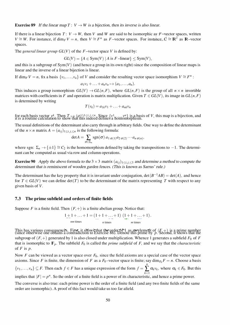
7/26/2019 MATH 2968 Algebra Advanced Notes
http://slidepdf.com/reader/full/math-2968-algebra-advanced-notes 50/110
Exercise 89 If the linear map T : V → W is a bijection, then its inverse is also linear.
If there is a linear bijection T : V → W , then V and W are said to be isomorphic as F –vector spaces, written
V ∼= W . For instance, if dimF V = n, then V ∼= F n as F –vector spaces. For instance, C ∼= IR2 as IR–vector
spaces.
The general linear group GL(V ) of the F –vector space V is defined by:
GL(V ) = A ∈ Sym(V ) | A is F –linear ≤ Sym(V ),
and this is a subgroup of Sym(V ) (and hence a group in its own right) since the composition of linear maps is
linear and the inverse of a linear bijection is linear.
If dimF V = n, fix a basis v1, . . . , vn of V and consider the resulting vector space isomorphism V ∼= F n :
a1v1 + . . . + anvn → (a1, . . . , an).
This induces a group isomorphism GL(V ) → GL(n, F ), where GL(n, F ) is the group of all n × n invertible
matrices with coefficients in F and operation is matrix multiplication. Given T ∈ GL(V ), its image in GL(n, F )is determined by writing
T (vk ) = a1k v1 + . . . + ank vn
for each basis vector vk . Then T → (ai j)1≤i, j,≤n. Since v1, . . . , vn is a basis of V , this map is a bijection, andit is a routine calculation to show that this indeed defines a homomorphism.
The usual definitions of the determinant also carry through in arbitrary fields. One way to define the determinant
of the n × n matrix A = (ai j)1≤i, j,≤n is the following formula:
det A = ∑σ ∈Σn
sgn(σ ) a1 σ (1)a2 σ (2) · · ·an σ (n),
where sgn: Σn →±1 ∼= C 2 is the homomorphism defined by taking the transpositions to −1. The determi-
nant can be computed as usual via row and column operations.
Exercise 90 Apply the above formula to the 3 ×3 matrix (ai j)1≤i, j,≤3 and determine a method to compute the
determinant that is reminiscent of wooden garden fences. (This is known as Sarrus’ rule.)
The determinant has the key property that it is invariant under conjugation, det ( B−1 AB) = det( A), and hence
for T ∈ GL(V ) we can define det(T ) to be the determinant of the matrix representing T with respect to any
given basis of V .
7.3 The prime subfield and orders of finite fields
Suppose F is a finite field. Then (F , +) is a finite abelian group. Notice that:
1 + 1 + . . . + 1
nm times
= (1 + 1 + . . . + 1)
n times
(1 + 1 + . . . + 1)
m times
.
This has various consequences. First, it shows that the order of 1 as an element of (F , +) is a prime number(since otherwise one obtains a contradiction to Exercise 86). Denote this prime by p. Second, it shows that the
subgroup of (F , +) generated by 1 is also closed under multiplication. Whence 1 generates a subfield F 0 of F
that is isomorphic to IF p. The subfield F 0 is called the prime subfield of F , and we say that the characteristic
of F is p.
Now F can be viewed as a vector space over F 0, since the field axioms are a special case of the vector space
axioms. Since F is finite, the dimension of F as a F 0 –vector space is finite; say dimF 0 F = n. Choose a basis
v1, . . . , vn ⊆ F . Then each f ∈ F has a unique expression of the form f =n
∑k =1
α k vk , where α k ∈ F 0. But this
implies that |F | = pn. So the order of a finite field is a power of its characteristic, and hence a prime power.
The converse is also true: each prime power is the order of a finite field (and any two finite fields of the same
order are isomorphic). A proof of this fact would take us too far afield.
50
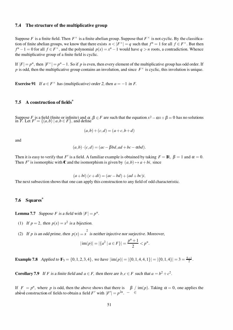
7/26/2019 MATH 2968 Algebra Advanced Notes
http://slidepdf.com/reader/full/math-2968-algebra-advanced-notes 51/110
7.4 The structure of the multiplicative group
Suppose F is a finite field. Then F × is a finite abelian group. Suppose that F × is not cyclic. By the classifica-
tion of finite abelian groups, we know that there exists n < |F ×| = q such that f n = 1 for all f ∈ F ×. But then
f n −1 = 0 for all f ∈ F ×, and the polynomial p( x) = xn −1 would have q > n roots, a contradiction. Whence
the multiplicative group of a finite field is cyclic.
If |F | = pn, then |F ×| = pn −1. So if p is even, then every element of the multiplicative group has odd order. If
p is odd, then the multiplicative group contains an involution, and since F × is cyclic, this involution is unique.
Exercise 91 If a ∈ F × has (multiplicative) order 2, then a = −1 in F .
7.5 A construction of fields*
Suppose F is a field (finite or infinite) and α ,β ∈ F are such that the equation x2 −α x +β = 0 has no solutionsin F . Let F = (a, b) | a, b ∈ F , and define
(a, b) + (c, d ) = (a + c, b + d )
and
(a, b) · (c, d ) = (ac −β bd , ad + bc −α bd ).
Then it is easy to verify that F is a field. A familiar example is obtained by taking F = IR, β = 1 and α = 0.Then F is isomorphic with C and the isomorphism is given by (a, b) → a + bi, since
(a + bi) (c + di) = (ac − bd ) + (ad + bc)i.
The next subsection shows that one can apply this construction to any field of odd characteristic.
7.6 Squares*
Lemma 7.7 Suppose F is a field with |F | = pn.
(1) If p = 2, then p( x) = x2 is a bijection.
(2) If p is an odd prime, then p( x) = x2
is neither injective nor surjective. Moreover,
| im( p)| = |a2 | a ∈ F | = pn + 1
2 < pn.
Example 7.8 Applied to IF5 = 0, 1, 2, 3, 4, we have | im( p)| = |0, 1, 4, 4, 1| = |0, 1, 4| = 3 = 5+12
.
Corollary 7.9 If F is a finite field and a ∈ F , then there are b, c ∈ F such that a = b2 + c2.
If |
F |
= pn, where p is odd, then the above shows that there is −
β /∈
im( p). Taking α = 0, one applies the
above construction of fields to obtain a field F with |F | = p2n.
51
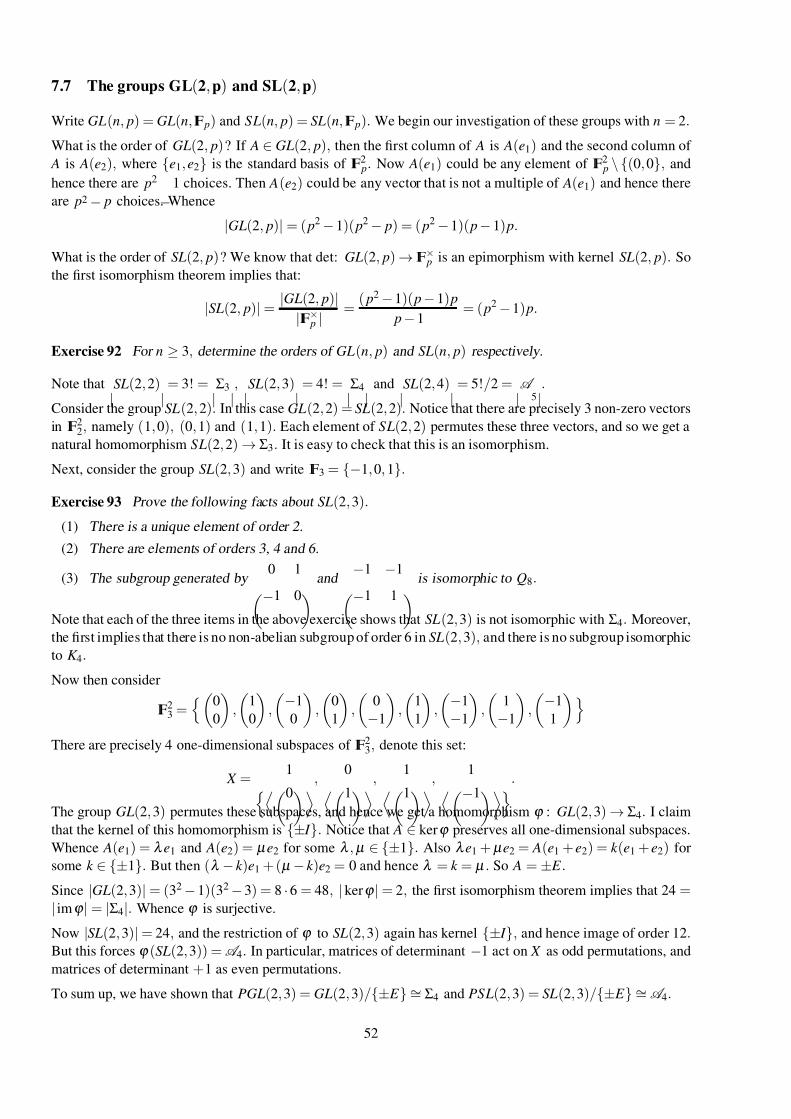
7/26/2019 MATH 2968 Algebra Advanced Notes
http://slidepdf.com/reader/full/math-2968-algebra-advanced-notes 52/110
7.7 The groups GL(2, p) and SL(2, p)
Write GL(n, p) = GL(n, IF p) and SL(n, p) = SL(n, IF p). We begin our investigation of these groups with n = 2.
What is the order of GL(2, p)? If A ∈ GL(2, p), then the first column of A is A(e1) and the second column of
A is A(e2), where e1, e2 is the standard basis of IF2 p. Now A(e1) could be any element of IF2
p \ (0, 0, and
hence there are p2
−1 choices. Then A(e2) could be any vector that is not a multiple of A(e1) and hence there
are p2 − p choices. Whence
|GL(2, p)| = ( p2 − 1)( p2 − p) = ( p2 −1)( p − 1) p.
What is the order of SL(2, p)? We know that det: GL(2, p) → IF× p is an epimorphism with kernel SL(2, p). So
the first isomorphism theorem implies that:
|SL(2, p)| = |GL(2, p)|
|IF× p | =
( p2 −1)( p − 1) p
p −1 = ( p2 −1) p.
Exercise 92 For n ≥ 3, determine the orders of GL(n, p) and SL(n, p) respectively.
Note that |
SL(2, 2)|
= 3! =|Σ3
|, |
SL(2, 3)|
= 4! =|Σ4
| and
|SL(2, 4)
|= 5!/2 =
|A
5|.
Consider the group SL(2, 2). In this case GL(2, 2) = SL(2, 2). Notice that there are precisely 3 non-zero vectors
in IF22, namely (1, 0), (0, 1) and (1, 1). Each element of SL(2, 2) permutes these three vectors, and so we get a
natural homomorphism SL(2, 2) → Σ3. It is easy to check that this is an isomorphism.
Next, consider the group SL(2, 3) and write IF3 = −1, 0, 1.
Exercise 93 Prove the following facts about SL(2, 3).
(1) There is a unique element of order 2.
(2) There are elements of orders 3, 4 and 6.
(3) The subgroup generated by 0 1
−1 0 and −1 −1
−1 1 is isomorphic to Q8.
Note that each of the three items in the above exercise shows that SL(2, 3) is not isomorphic with Σ4. Moreover,
the first implies that there is no non-abelian subgroup of order 6 in SL(2, 3), and there is no subgroup isomorphic
to K 4.
Now then consider
IF23 =
0
0
,
1
0
,
−1
0
,
0
1
,
0
−1
,
1
1
,
−1
−1
,
1
−1
,
−1
1
There are precisely 4 one-dimensional subspaces of IF2
3, denote this set:
X = 1
0, 0
1, 1
1, 1
−1.
The group GL(2, 3) permutes these subspaces, and hence we get a homomorphism ϕ : GL(2, 3) → Σ4. I claim
that the kernel of this homomorphism is ± I . Notice that A ∈ kerϕ preserves all one-dimensional subspaces.
Whence A(e1) = λ e1 and A(e2) = µ e2 for some λ ,µ ∈ ±1. Also λ e1 +µ e2 = A(e1 + e2) = k (e1 + e2) for
some k ∈ ±1. But then (λ − k )e1 + (µ − k )e2 = 0 and hence λ = k = µ . So A = ± E .
Since |GL(2, 3)| = (32 − 1)(32 −3) = 8 · 6 = 48, | kerϕ | = 2, the first isomorphism theorem implies that 24 =| imϕ | = |Σ4|. Whence ϕ is surjective.
Now |SL(2, 3)| = 24, and the restriction of ϕ to SL(2, 3) again has kernel ± I , and hence image of order 12.But this forces ϕ (SL(2, 3)) =A 4. In particular, matrices of determinant −1 act on X as odd permutations, and
matrices of determinant +1 as even permutations.
To sum up, we have shown that PGL(2, 3) = GL(2, 3)/± E ∼= Σ4 and PSL(2, 3) = SL(2, 3)/± E ∼=A 4.
52
7/26/2019 MATH 2968 Algebra Advanced Notes
http://slidepdf.com/reader/full/math-2968-algebra-advanced-notes 53/110
Remark 7.10 Recall that PGL(n, F ) = GL(n, F )/ Z (GL(n, F )), where Z (GL(n, F )) = α E |α ∈ F ×. Simi-
larly, PSL(n, F ) = SL(n, F )/ Z (SL(n, F )), where Z (SL(n, F )) = α E |α n = 1.
Exercise 94 Show that SL(2, 4) ∼= PSL(2, 4) ∼=A 5.
Remark 7.11 Given a vector space V , the set of all one-dimensional subspaces P(V ) is called a projectivespace. In the above example, V = IF2
3 and P(V ) = X . The groups GL(V ) and SL(V ) act on P(V ), but their ac-
tion may not be effective. This is the reason why one passes to the induced projective linear groups PGL(V ) and
PSL(V ), which do act effectively on P(V ). The study of projective spaces goes back to perspective drawings
by Renaissance artists such as Albrecht D urer and Leonardo da Vinci.
7.8 More about SL(2, 3)
We will now use the Sylow theorems to determine how many elements of each order are contained in SL(2, 3).We have
|SL(2, 3)
|= 24 = 23 3. Whence
|Syl3(SL(2, 3))
| ∈ 1, 4
and
|Syl2(SL(2, 3))
| ∈ 1, 3
.
Now the elements 1 1
0 1
and
1 0
1 1
have order 3 and generate distinct subgroups of order 3. So |Syl3(SL(2, 3))| = 4. Moreover, any two distinct
subgroups of order 3 only meet in the identity. Hence there are precisely 8 elements of order 3 in SL(2, 3).Multiplying an element of order 3 by − E gives an element of order 6. Hence there are at least 8 elements of
order 6. We also have a subgroup isomorphic to Q8,
0 1
−1 0
,
−1 −1
−1 1
∼= Q8,
and this contains no element of order 3 or 6. But 8 + 8 + 8 = 24, and hence we have counted all elements of
SL(2, 3). The quaternion group has precisely one element each of order 1 and 2, and 6 elements of order 4. To
sum up, the number of elements of each order in SL(2, 3) is as follows:
order 1 2 3 4 6
number of elements 1 1 8 6 8
This count also shows that |Syl2(SL(2, 3))| = 1, and hence the quaternion subgroup of SL(2, 3) is normal.
Exercise 95 The conjugacy classes partition a group. Determine all conjugacy classes in SL(2, 3).
7.9 Some p–groups
Let
U =1 a b
0 1 c
0 0 1
a, b, c ∈ IF p
≤ SL(3, p) ≤ GL(3, p).
Then |U | = p3, and U is a p–group.
Exercise 96 If p = 2, then U ∼= D4.
53
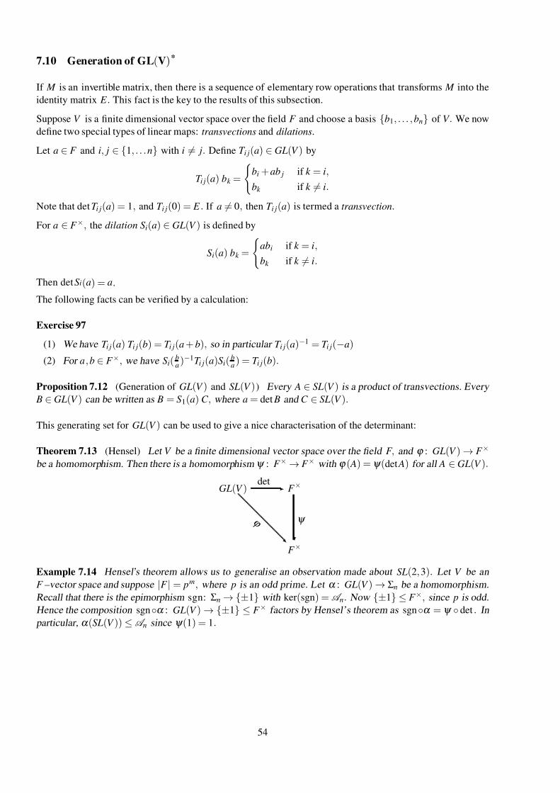
7/26/2019 MATH 2968 Algebra Advanced Notes
http://slidepdf.com/reader/full/math-2968-algebra-advanced-notes 54/110
7.10 Generation of GL(V)*
If M is an invertible matrix, then there is a sequence of elementary row operations that transforms M into the
identity matrix E . This fact is the key to the results of this subsection.
Suppose V is a finite dimensional vector space over the field F and choose a basis b1, . . . , bn of V . We now
define two special types of linear maps: transvections and dilations.
Let a ∈ F and i, j ∈ 1, . . . n with i = j. Define T i j(a) ∈ GL(V ) by
T i j(a) bk =
bi + ab j if k = i,
bk if k = i.
Note that det T i j(a) = 1, and T i j(0) = E . If a = 0, then T i j(a) is termed a transvection.
For a ∈ F ×, the dilation S i(a) ∈ GL(V ) is defined by
S i(a) bk =
abi if k = i,
bk if k = i.
Then det S i(a) = a.
The following facts can be verified by a calculation:
Exercise 97
(1) We have T i j(a) T i j(b) = T i j(a + b), so in particular T i j(a)−1 = T i j(−a)
(2) For a, b ∈ F ×, we have S i(ba
)−1T i j(a)S i(ba
) = T i j(b).
Proposition 7.12 (Generation of GL(V ) and SL(V )) Every A ∈ SL(V ) is a product of transvections. Every
B ∈ GL(V ) can be written as B = S 1(a) C , where a = det B and C ∈ SL(V ).
This generating set for GL(V ) can be used to give a nice characterisation of the determinant:
Theorem 7.13 (Hensel) Let V be a finite dimensional vector space over the field F , and ϕ : GL(V ) → F ×
be a homomorphism. Then there is a homomorphism ψ : F × → F × with ϕ ( A) = ψ (det A) for all A ∈ GL(V ).
GL(V ) det F ×
ϕ
F ×
ψ
Example 7.14 Hensel’s theorem allows us to generalise an observation made about SL(2, 3). Let V be an
F –vector space and suppose |F | = pm, where p is an odd prime. Let α : GL(V ) → Σn be a homomorphism.
Recall that there is the epimorphism sgn: Σn → ±1 with ker(sgn) =A n. Now ±1 ≤ F ×, since p is odd.
Hence the composition sgnα : GL(V ) → ±1 ≤ F × factors by Hensel’s theorem as sgnα = ψ det . In
particular, α (SL(V )) ≤A n since ψ (1) = 1.
54
7/26/2019 MATH 2968 Algebra Advanced Notes
http://slidepdf.com/reader/full/math-2968-algebra-advanced-notes 55/110
8 Normal forms for linear maps
This section studies linear transformations on a finite dimensional vector space via their minimal polynomial
and invariant subspaces. This leads to the Jordan Normal Form for linear transformations, and a proof of the
Cayley-Hamilton theorem, which states that every linear map satisfies its characteristic equation. In doing so,
important concepts concerning vector spaces are introduced such as complementary subspaces and quotient
spaces.
8.1 A remark on bases
A basis of a vector space is usually defined to be a linearly independent spanning set. In this section, we will
term this an unordered basis and write it as a set, such as v j | j ∈Λ where Λ is some index set. The cardinality
of Λ is the dimension of the vector space. A basis will mean an ordered basis, written (v j | j ∈ Λ), where the
ordering comes from a natural ordering of Λ, or the vectors are explicitly listed in order, such as (u, v, w). Note
that if dimV = 3 and u, v, w is an unordered basis of V , then u, v, w = u, w, v = u, w, w, v, so each of
these sets is the same unordered basis, but (u, v, w) are (u, w, v) are different ordered bases, and (u, w, w, v) is
not an ordered basis.
For a finite dimensional vector space, it is relatively easy to establish the existence of basis and the fact that any
two bases have the same number of elements. This is a different story for infinite dimensional vector spaces.
Using the axiom of choice, it is usually shown that every vector space has an unordered basis and that any
two bases have the same cardinality. Applying the axiom of choice again, one can order any basis. So in
particular, a vector space such as the space C [a, b] of all continuous functions f : [a, b] → IR has an ordered
basis ( f j | j ∈Λ), where the cardinality of Λ is 2ℵ0 , the same as the cardinality of IR. We have a preferred
ordering of the reals, and any bijection C [a, b] → IR will gives us an ordering on C [a, b]. But how do you get
your hands on such a bijection?
This section is devoted to the study of linear transformations on finite dimensional vector spaces. Some of
below results or definitions hold verbatim in the general setting (though often with different proofs). The
guiding principle will be the search for a basis which gives a good understanding of ϕ , or which has other
advantages in the study or application of ϕ . We will mainly focus on choosing a basis for just one linear
transformation.
8.2 Choosing a basis
Case study 1: Given ϕ : V → V , suppose there is a basis B of V such that [ϕ ]B is a diagonal matrix, i.e.
[ϕ ]B =
d 1 0 · · · · · · 0
0 d 2 . . . .
.....
. . . . . .
. . . ...
... . . .
. . . 0
0 0 · · · 0 d n
,
where the only non-zero entries are on the diagonal. It is then very easy to compute the image of [v]B under
[ϕ ]B , and to take arbitrary powers of [ϕ ]B . We also completely understand how [ϕ ]B acts on F n : the coordi-
nate direction ek is dilated or collapsed, depending on whether d k is non-zero or zero. The basis B consists of
eigenvectors of ϕ , and we can read off the dimension of each eigenspace (including the kernel of ϕ ) from the
diagonal entries. It is also easy to determine invariants of ϕ , such as the determinant, and we have many nice
algebraic properties, such as [ϕ ]B is symmetric. The diagonal form allows us to both understand ϕ well, and
to do computations.
55
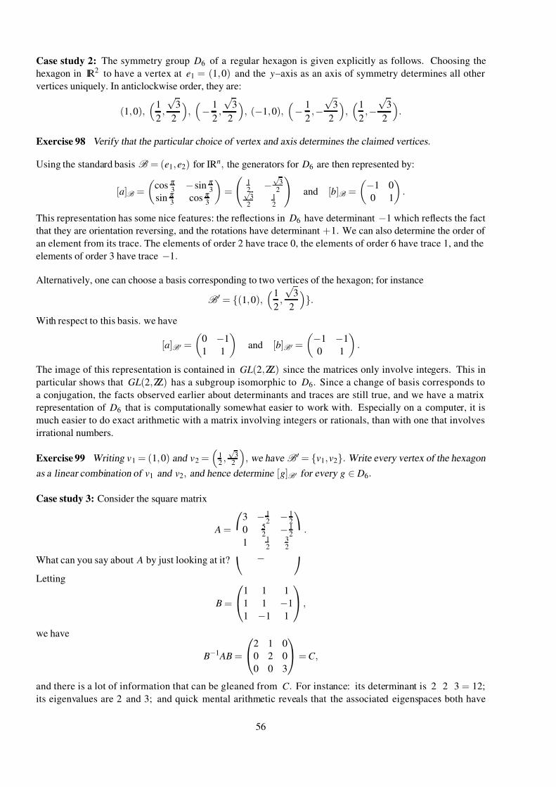
7/26/2019 MATH 2968 Algebra Advanced Notes
http://slidepdf.com/reader/full/math-2968-algebra-advanced-notes 56/110
Case study 2: The symmetry group D6 of a regular hexagon is given explicitly as follows. Choosing the
hexagon in IR2 to have a vertex at e1 = (1, 0) and the y–axis as an axis of symmetry determines all other
vertices uniquely. In anticlockwise order, they are:
(1, 0),1
2,
√ 3
2
,
− 1
2,
√ 3
2
, (−1, 0),
− 1
2,−
√ 3
2
,1
2,−
√ 3
2
.
Exercise 98 Verify that the particular choice of vertex and axis determines the claimed vertices.
Using the standard basis B = (e1, e2) for IRn, the generators for D6 are then represented by:
[a]B =
cos π
3 −sin π
3
sin π 3
cos π 3
=
1
2 −
√ 3
2√ 3
212
and [b]B =
−1 0
0 1
.
This representation has some nice features: the reflections in D6 have determinant −1 which reflects the fact
that they are orientation reversing, and the rotations have determinant +1. We can also determine the order of
an element from its trace. The elements of order 2 have trace 0, the elements of order 6 have trace 1, and the
elements of order 3 have trace −1.
Alternatively, one can choose a basis corresponding to two vertices of the hexagon; for instance
B = (1, 0),
1
2,
√ 3
2
.
With respect to this basis. we have
[a]B =
0 −1
1 1
and [b]B =
−1 −1
0 1
.
The image of this representation is contained in GL(2, ZZ) since the matrices only involve integers. This in
particular shows that GL(2, ZZ) has a subgroup isomorphic to D6. Since a change of basis corresponds to
a conjugation, the facts observed earlier about determinants and traces are still true, and we have a matrix
representation of D6 that is computationally somewhat easier to work with. Especially on a computer, it is
much easier to do exact arithmetic with a matrix involving integers or rationals, than with one that involves
irrational numbers.
Exercise 99 Writing v1 = (1, 0) and v2 =
12
,√
32
, we have B = v1, v2. Write every vertex of the hexagon
as a linear combination of v1 and v2, and hence determine [g]B for every g ∈ D6.
Case study 3: Consider the square matrix
A =
3 − 1
2 − 1
2
0 52
− 12
1
−12
32
.
What can you say about A by just looking at it?
Letting
B =
1 1 1
1 1 −1
1 −1 1
,
we have
B−1 AB =
2 1 0
0 2 0
0 0 3
= C ,
and there is a lot of information that can be gleaned from C . For instance: its determinant is 2·
2·
3 = 12;
its eigenvalues are 2 and 3; and quick mental arithmetic reveals that the associated eigenspaces both have
56
7/26/2019 MATH 2968 Algebra Advanced Notes
http://slidepdf.com/reader/full/math-2968-algebra-advanced-notes 57/110
dimension 1. In particular, the matrix A is not diagonalisable. It also shows that there are two invariant
subspaces of IR3, one of dimension 2 and the other of dimension 1, and that these subspaces are complementary.
One can also read off the characteristic polynomial. All of these properties of C are invariant under conjugation,
and hence hold for A.
The matrix C is the so-called Jordan Normal Form of A. The remainder of this section will answer the ques-
tions: Under which conditions can we put a matrix into such a nice form? What is the best we can hope for?
How can we find a normal form of a matrix?
We will address these questions in the general framework of linear transformations on vector spaces. Matrices
appear in this setting as representations of transformations by choosing bases for the vector spaces.
Exercise 100 This exercise is intended to refresh some techniques from linear algebra. Verify B−1 AB = C
without computing the inverse of B. Does your verification imply that B is indeed invertible? If not, establish
that B is invertible. Determine B−1. The matrix A defines a linear transformation ϕ : IR3 → IR3 by ϕ ( x) = Ax.So [ϕ ]B = A, where B is the standard basis of IR3. Show that there is a basis B such that [ϕ ]B = C and
determine B .
8.3 Eigenvalues and the characteristic polynomial
Recall that HomF (V ,V ) is the set of all F –linear transformations ϕ : V → V . If there are 0 = v ∈ V and λ ∈ F
such that ϕ (v) =λ v, then λ is an eigenvalue of ϕ and v is an eigenvector of ϕ corresponding to the eigenvalue
λ . The set
E ϕ (λ ) = v ∈ V | ϕ (v) = λ vis the eigenspace of ϕ corresponding to the eigenvalue λ . This consists of all eigenvectors of ϕ corresponding
to λ and the zero vector (which is not considered to be an eigenvector).
Example 8.1 A reflection ρ in a line through the origin in IR2 has the eigenvalues −1 and +1. The eigenspace
E ρ(1) is the line of reflection; the eigenspace E ρ(−1) is the line through the origin that is perpendicular to the line of reflection.
Example 8.2 Let V = C ∞(IR) be the real vector space of all real-valued functions on IR that are differentiable
infinitely often. Then differentiation is a linear transformation on C ∞(IR). Since d dx
eλ x = λ eλ x, differentiation
has every real number as an eigenvalue with corresponding eigenvector eλ x.
Eigenvectors corresponding to different eigenvalues are linearly independent: If ϕ (wk ) = λ k wk and λ k = λ j for
all 1 ≤ k , j ≤ m, then w1, . . . , wm is linearly independent in V .
Definition 8.3 The characteristic polynomial of ϕ ∈ HomF (V ,V ) is the polynomial cϕ ( x) = det( xe −ϕ ).
Now λ ∈ F is an eigenvalue if and only if (λ e −ϕ ) has non-trivial kernel if and only if det(λ e −ϕ ) = 0. So
the eigenvalues of ϕ are precisely the zeros of its characteristic polynomial. We have E ϕ (λ ) = ker(λ e −ϕ ).If λ ∈ F is an eigenvalue of ϕ , then dim E ϕ (λ ) is the geometric multiplicity of λ . If ( x −λ )k is the highest
power of x −λ dividing cϕ , then k is termed the algebraic multiplicity of λ . Choosing an appropriate basis of
V , it is easy to see that:
(geometric multiplicity of λ ) ≤ (algebraic multiplicity of λ )
for each eigenvalue λ of ϕ . If V has a basis B consisting of eigenvectors of ϕ , then [ϕ ]B is a diagonal matrix.
In this case, ϕ is called diagonalisable. This is the best one can hope for in representing a linear transformation,
and the above gives a simple test: ϕ is diagonalisable if and only if its characteristic polynomial has dimV zeros
(counted with multiplicity) and for each of these zeros, the geometric multiplicity and the algebraic multiplicity
are equal.
57
7/26/2019 MATH 2968 Algebra Advanced Notes
http://slidepdf.com/reader/full/math-2968-algebra-advanced-notes 58/110
8.4 Invariant subspaces and complements
Notice that ϕ ( E ϕ (λ )) ≤ E ϕ (λ ), since if v ∈ E ϕ (λ ), then ϕ (v) = λ v, and so ϕ (ϕ (v)) = ϕ (λ v) = λϕ (v), and
so ϕ (v) ∈ E ϕ (λ ). We will decorate such subspaces with the appropriate adjective:
Definition 8.4 Let ϕ : V → V be a linear transformation and suppose that W ≤ V is a subspace. Then W is
ϕ –invariant if ϕ (W ) ≤ W .
Exercise 101 When is ϕ ( E ϕ (λ )) = E ϕ (λ )?
If W ≤ V is a ϕ –invariant subspace, then ϕ restricts to a linear map ϕ W = ϕ |W : W → W . Suppose that
V is finite dimensional with dim(V ) = n. Any basis B W = (w1, . . . wm) of W can be extended to a basis
B = (w1, . . . wm, vm+1, . . . , vn). With respect to this basis, ϕ has the matrix
[ϕ ]B =
[ϕ W ]B W
B
0 A
,
where A is an (
n−
m)× (
n−
m)
matrix and 0 is the (
n−
m) ×
m zero-matrix.
Example 8.5 Suppose ϕ : IR3 → IR3 is a rotation about a line L through the origin. The plane P through the
origin and perpendicular to L is a ϕ –invariant subspace of IR3. Choosing two orthogonal vectors u and v in P
that have the same length, and a vector w ∈ IR3 \ P, we obtain the basis B = (u, v, w) of IR3. Then
[ϕ ]B =
cosϑ −sinϑ a
sinϑ cosϑ b
0 0 1
,
where ϑ ∈ [0, 2π ) depends on the component of IR2 \ P containing w. Choosing w in the other component
changes the angle to 2π −ϑ unless ϑ = 0. Also note that a = 0 = b if and only if w ∈ L, and this gives the
nicest form for [ϕ ]B .
The example leads us to the next concept.
Definition 8.6 Suppose W ≤ V . Then U ≤ V is a complement to W if U ∩W = 0 and U +W = V . This is
written V = U ⊕W , and we say that U and W are complementary subspaces and that V is the (internal) direct
sum of U and W .
Note that U and W are complementary subspaces if and only if the additive abelian group V (forgetting the
extra structure of an F –vector space) is the internal direct product of U and W . The notation U ⊕W agrees
with the convention that if U and V are abelian groups with additive notation for the group operation, then we
write U
⊕W = U
×V . Also note that
0
and V are complementary subspaces.
Exercise 102 Let V be a finite dimensional vector space and W ≤ V . Show that W has a complement in V .
Lemma 8.7 Suppose V = U ⊕W , and B U is an unordered basis of U and B W an unordered basis of W .Then B =B U ∪B W is an unordered basis of V .
Exercise 103 Let V be a finite dimensional vector space. Suppose the linear transformation ϕ : V → V has
the ϕ –invariant subspaces U and W , and that V = U ⊕W . Choose a basis B U of U and a basis B W of W ,and let B = (B U ,B W ). This is a basis of V by Lemma 8.7. Show that [ϕ ]B has the block diagonal form:
[ϕ ]B = [ϕ U ]B U 0
0 [ϕ W ]B W
.
58
7/26/2019 MATH 2968 Algebra Advanced Notes
http://slidepdf.com/reader/full/math-2968-algebra-advanced-notes 59/110
In this case, we say that ϕ is the direct sum of ϕ U and ϕ W , written ϕ = ϕ U ⊕ϕ W . We will also apply the direct
sum notation to matrices, and write:
[ϕ U ]B U ⊕[ϕ W ]B W
=
[ϕ U ]B U
0
0 [ϕ W ]B W
.
If both ϕ : V →
V and ψ : V →
V leave the complementary subspaces U and W invariant, then we have
[ϕψ ]B = [ϕ U ψ U ]B U ⊕[ϕ W ψ W ]B W
=
[ϕ U ]B U
0
0 [ϕ W ]B W
[ψ U ]B U
0
0 [ψ W ]B W
.
Remark 8.8 Similar to the case of groups, given F –vector spaces U and W , we can form their (external)
direct sum U ⊕W by taking as set of elements the set of ordered pairs (u, w) | u ∈ U , w ∈ W and using the
natural operations (u1, w1) + (u2, w2) = (u1 + u2, w1 + w2) and a(u, w) = (au, aw).
If ϕ : U →U and ψ : W → W are linear transformations, then their (external) direct sum is the transformation
ϕ ⊕ψ : U ⊕W → U ⊕W
defined by (ϕ ⊕ψ )(u, w) = (ϕ (v),ψ (w)).
8.5 Quotient spaces*
The notion of a quotient space is as fundamental to the theory of vector spaces as the notion of a quotient group
to group theory. In the case of finite dimensional vector spaces, this will enable us to give proofs by induction
on the dimension of a vector space; just as we were able to give proofs by induction on the order of a group in
some results about finite groups.
Suppose V is an F –vector space and W ≤ V a subspace. Ignoring the extra structure of the vector space,
consider V as an abelian group. Then W is a normal subgroup, and hence we may form the quotient group
V /W with set of elements the cosets of W , v +W | v ∈ V and operation
(v1 +W ) + (v2 +W ) = (v1 + v2) +W .
The identity in this group is W = 0 +W and the inverse of v +W is −v +W . We now turn the abelian group
V /W into an F –vector space by defining
a(v +W ) = av +W .
This multiplication by scalars is well-defined: If v1 +W = v2 +W , then v1 − v2 ∈ W . Since W is a subspace,
we have a(v1 − v2) ∈ W for each a ∈ F , and so av1 +W = av2 +W for each a ∈ F .
Exercise 104 Verify that the vector space axioms are satisfied. You already know that V /W is a group, so the
only properties to check are 2(a)–(d) in Definition 7.6.
Proposition 8.9 Suppose V is an F –vector space and W ≤ V a subspace.
(1) Given an unordered basis w j | j ∈ Λ of W and an unordered basis vk + W | k ∈ Ω of V /W , where
Λ and Ω are arbitrary index sets, then w j, vk | j ∈ Λ, k ∈Ω is an unordered basis of V .
(2) If V is finite dimensional, then dimV /W = dim V − dimW .
Exercise 105 Let V be a finite dimensional vector space.
(1) Suppose (v1, . . . , vn) is a basis of V and let W = v1, . . . , vm.Show that (vm+1 +W , . . . , vn +W ) is a basis of V /W .
(2) Deduce that any subspace U ≤ V has a complement in V that is isomorphic to V /U .
59
7/26/2019 MATH 2968 Algebra Advanced Notes
http://slidepdf.com/reader/full/math-2968-algebra-advanced-notes 60/110
Suppose ϕ : V →V is a linear map, and let W = ker(ϕ ). Then we get an induced linear map ϕ : V /W →V /W
defined by
ϕ (v +W ) = ϕ (v) +W .
Exercise 106 Show that ϕ is well-defined and linear.
Example 8.10 Consider the map ϕ : F 2 → F 2 defined by ϕ ( x, y) = ( y, 0). Then W = ker(ϕ ) = (1, 0) and
F 2/W = (0, y) +W | y ∈ F . Now ϕ ( (0, y) +W ) = (0, 0) +W = W , and so ϕ = 0 ∈ HomF (V /W ,V /W ).
8.6 The minimal polynomial
Given a polynomial p ∈ F [ x] and an F –linear transformation ϕ : V →V , we obtain a new linear transformation
p(ϕ ) : V → V as follows. Writing p( x) = ∑mk =0 ak x
k , where ak ∈ F , we define
p(ϕ ) =m
∑k =0
ak ϕ k ∈ HomF (V ,V ),
where ϕ 0 = e : V → V is the identity map. If p(ϕ ) = 0 ∈ HomF (V ,V ) is the zero-map, then we say that ϕ is
a zero of p in HomF (V ,V ). We will also just say that ϕ is a zero of p if it is clear from the context whether a
zero of p in F or a zero of p in HomF (V ,V ) is meant.
Example 8.11 Let ϕ : IR2 → IR2 be the anti-clockwise rotation by π 2
about the origin and p( x) = x3 + x. Then
p(ϕ ) = ϕ 3 +ϕ . Now
p(ϕ )(v) = ϕ 3(v) +ϕ (v) = ϕ −1(v) +ϕ (v) = −ϕ (v) +ϕ (v) = 0 ∈ IR2
for each v ∈ IR2. In particular, p(ϕ ) = 0 ∈ HomF (V ,V ). Also note that p( x) = x( x2 + 1), and since ϕ 2 = −e,
we also have q(ϕ ) = 0 with q( x) = x2
+ 1.
Exercise 107 Let p, q ∈ F [ x] and ϕ ∈ HomF (V ,V ).
(1) Show that p(ϕ ) : V → V is an F –linear transformation.
(2) Show that p(ϕ )q(ϕ ) = q(ϕ ) p(ϕ ); i.e. the two linear transformations commute.
A polynomial is monic if its leading coefficient is 1. For instance, p( x) = x3 + x.
Definition 8.12 Let ϕ ∈ HomF (V ,V ). We call p ∈ F [ x] the minimal polynomial of ϕ and write mϕ = p, if p
is the monic polynomial of smallest degree such that p(ϕ ) = 0 ∈ HomF (V ,V ).
The statement of the definition assumes existence and uniqueness of such a polynomial. Existence of mϕ fol-
lows from the fact that HomF (V ,V ) has finite dimension, and so the set e,ϕ ,ϕ 2, . . . ,ϕ n, . . . ,ϕ nn
, . . . is not
linearly independent. Whence there are m ∈ IN and ak ∈ F (not all equal to zero) such that ∑mk =0 ak ϕ
k = 0.Letting p( x) =∑
mk =0 ak x
k , we have p(ϕ ) = 0. We may assume am = 0, and so 1am
p is a monic polynomial hav-
ing ϕ as a zero. Using the well-ordering principle, there is a monic polynomial of smallest degree. Uniqueness
follows from the fact that the difference of two such monic polynomials p and q of smallest degree satisfies
deg( p − q) < deg( p) = deg(q) and ( p− q)(ϕ ) = p(ϕ )− q(ϕ ) = 0 −0 = 0. Whence p − q = 0 and so p = q.
Example 8.13 Suppose ρ : IR2
→IR2 is a reflection in a line through the origin. Then ρ2 = e hence ρ is a
zero of the polynomial x2 −1. Since ρ = ae for every a ∈ IR, we have mρ( x) = x2 − 1.
60
7/26/2019 MATH 2968 Algebra Advanced Notes
http://slidepdf.com/reader/full/math-2968-algebra-advanced-notes 61/110
Example 8.14 Suppose ϕ : V → V is a linear isomorphism of order 3. Then ϕ 3 = e, and hence ϕ is a zero
of the polynomial x3 − 1. Now x3 − 1 = ( x − 1)( x2 + x + 1). If ϕ = e, then ϕ is a zero of x2 + x + 1. If
x2 + x + 1 is not minimal, then mϕ has degree 1 and is of the form mϕ ( x) = x − a with some a ∈ F ×. Then
0 = mϕ (ϕ ) = ϕ − ae and hence ϕ = ae. Since e = ϕ 3 = a3e, we have a3 = 1, and in particular F × contains
an element of order 3.
Now if
|F
| is finite, then Lagrange’s theorem and Cauchy’s theorem imply that F × contains such an element
if and only if |F | ≡ 1 mod 3. For instance, it is a pleasant exercise in basic number theory to show that if
|F | = p2n, where p is a prime distinct from 3, then |F | ≡ 1 mod 3. If |F | is infinite, there are other possibilities
(such as F = C). To sum up, either mϕ ( x) = x − a with a an element of order 3 in F ×, or mϕ ( x) = x2 + x + 1.
An example with mϕ ( x) = x − a is the C–linear map ϕ : C → C defined by ϕ ( z) = e2π i/3 z. Here a = e2π i/3.An example with mρ( x) = x2 + x + 1 is the IR–linear map ρ : IR2 → IR2 defined by:
ρ
x
y
=
cos 2π
3 −sin 2π
3
sin 2π 3
cos 2π 3
x
y
,
a rotation by 2π /3 about the origin of IR2. If you ignore the algebraic structure and identify C with IR2 by
z = x + iy ≡ ( x, y) ∈ IR2, then ϕ and ρ are the same map. However, the algebraic differences are reflected in
the polynomials; ϕ has one eigenvalue with eigenspace all of C whilst ρ has no eigenvectors in IR2.
Lemma 8.15 If ϕ : V → V is a zero of q ∈ F [ x], then mϕ divides q.
Example 8.16 In the previous example, ϕ ( z) = e2π i/3 z is a zero of q( x) = x2 + x + 1 and mϕ ( x) = x − e2π i/3.Now q( x) = x2 + x + 1 = ( x −e2π i/3)( x −e−2π i/3) = mϕ ( x)( x −e−2π i/3).
Once some polynomial p is known that has ϕ as a zero, the above lemma implies that mϕ can be determined
from p. For instance, given the map ϕ : IR3 → IR3 defined by ϕ ( x) = Cx, where
C =
2 1 0
0 2 0
0 0 3
,
it is easy to check that ϕ is a zero of p( x) = ( x − 2)2
( x −3). Whence the possibilities for mϕ are
mϕ ( x) =
( x −2)2( x − 3)
( x −2)2
( x −2)( x − 3)
( x −2)
( x −3)
By inspection ϕ = 2e and ϕ = 3e, and this rules out the last three possibilities. A quick calculation shows
(ϕ − 2e)2 = 0, and hence mϕ = p. The following lemma limits the number of initial possibilities even more:
Lemma 8.17 The zeros of mϕ in F are exactly the eigenvalues of ϕ .
In the above examples, the minimal polynomial was obtained by starting with some polynomial having ϕ as a
zero. Here is another method that is sometimes useful:
Lemma 8.18 Suppose ϕ : V → V is a linear transformation and V = W 1 + . . . +W m, where each subspace W k
is ϕ –invariant. Suppose mk is the minimal polynomial of the restriction of ϕ to W k . Then
mϕ = lcm(m1, . . . mm).
Note that the above lemma merely assumes a sum ( +), not a direct sum (⊕), so W j ∩W k may be non-trivial.
Exercise 108 Show that ϕ ∈ GL(V ) if and only if its minimal polynomial has non-zero constant term.
Exercise 109 Suppose that ϕ
∈HomF (V ,V ) and p(ϕ ) = 0 for some p
∈F [ x] with non-zero constant term.
Show that ϕ is invertible.
61
7/26/2019 MATH 2968 Algebra Advanced Notes
http://slidepdf.com/reader/full/math-2968-algebra-advanced-notes 62/110
8.7 Some facts about polynomials
Since a field has no zero-divisors, the ring F [ x] of all polynomials with coefficients in F has the property that
if p and q are two non-zero-polynomials, then pq is also a non-zero polynomial. The degree of a polynomial
is defined in the usual fashion: If p( x) = ∑ak xk , then
deg p = max
k |
ak
= 0
.
A useful convention for the zero-polynomial is deg0 = max / 0 = −∞. We perform arithmetic using the conven-
tions (−∞) + (−∞) = (−∞), and n + (−∞) = −∞ for all n ∈ IN, and extend the order on IN to IN ∪−∞ by
defining −∞< n for all n ∈ IN. In particular, we always have the inequality
deg( p + q) ≤ maxdeg( p), deg(q),
and the equality
deg( pq) = deg( p) + deg(q).
Gauß observed that division with remainder and greatest common divisors apply in F [ x], with the same conse-
quences as for the integers.
Division with remainder 8.19 Let p, q ∈ F [ x] with q = 0. Then there exist polynomials r , s ∈ F [ x] with
p = sq + r ,
where either r = 0 or deg(r ) < deg(q). Moreover, r and s are uniquely determined by p and q.
The uniqueness of s and r is clear. To prove existence, there are three cases. If deg(q) > deg( p), one simply
takes s = 0 and r = p. If deg(q) = deg( p), then s is the ratio of the leading coefficients of p and q, and hence
r is obtained by taking p− sq. So the interesting case is when deg(q) < deg( p). In this case, the result follows
by using the familiar long division of polynomials.
The degree of a polynomial does not give a total order on the set of all polynomials, but it is good enough to
show that the Euclidean algorithm and the extended Euclidean algorithm can be applied to elements of F [ x].However, since all constants have degree 0, just as in the definition of the minimal polynomial, one needs to
normalise polynomials in order to get uniqueness statements.
Greatest common divisor 8.20 Let p, q ∈ F [ x]. There exists a unique monic polynomial d ∈ F [ x] such that
(1) d divides both p and q, and
(2) if r divides both p and q, then r divides d .
The polynomial d is called the greatest common divisor of p and q, written d = gcd( p, q). If d = 1, then p
and q are co-prime.
In analogy, the least common multiple of a finite set of elements S in F [ x] is defined to be the monic polynomial
of smallest degree, denoted lcm(S ), with the property that each element in S divides lcm(S ).
8.8 Polynomials and invariant subspaces
The observation that the eigenspaces of a linear transformation are invariant subspaces has a vast generalisation:
Lemma 8.21 Suppose ϕ ∈ HomF (V ,V ) and p ∈ F [ x] is any polynomial. Then ker( p(ϕ )) is ϕ –invariant.
Example 8.22 If λ is an eigenvalue of ϕ , then E ϕ (λ ) = ker( p(ϕ )), where p( x) = x −λ .
62
7/26/2019 MATH 2968 Algebra Advanced Notes
http://slidepdf.com/reader/full/math-2968-algebra-advanced-notes 63/110
Example 8.23 For the rotation from Example 8.5, we have P = ker( p(ϕ )), where p( x) = x2 − 2cosϑ + 1,and L = ker(q(ϕ )), where q( x) = x − 1.
Given co-prime integers a and b, the extended Euclidean algorithm determines integers c and d such that
ad + bc = 1. In the same fashion, given co-prime polynomials p and q, the extended Euclidean algorithm will
determine polynomials s, t ∈ F [ x] such that ps + qt = 1 ∈ F [ x]. This is the heart of the following result:
Lemma 8.24 Let ϕ : V → V be a linear transformation and suppose p ∈ F [ x] has the property that p(ϕ ) = 0.Also suppose that p = qr , where q and r are not constant and co-prime. Then V = ker(q(ϕ )) ⊕ker(r (ϕ )).
Combining the above lemma with Exercise 103, an easy induction gives the following result:
Proposition 8.25 Let ϕ : V → V be a linear transformation and suppose
mϕ =m
∏k =1
( pk )sk ,
where sk ∈ IN, each pk ∈ F [ x] is irreducible, monic and pk = p j for all k = j. Let W k = ker(( pk (ϕ ))sk ) and
write ϕ k = ϕ W K . for the restriction of ϕ to W k . Then
V = W 1 ⊕ . . .⊕W m,
and ϕ is the direct sum of its restrictions:
ϕ = ϕ 1 ⊕ . . .⊕ϕ m.
In particular, choosing a basis B k for W k , then B = (B 1, . . . ,B m) is a basis for V and we have the following
block diagonal matrix:
[ϕ ]B = [ϕ 1]B 1 ⊕ . . .⊕ [ϕ m]B m =
[ϕ 1]B 1 0 · · · · · · · · · 0
0 [ϕ 2]B 2 0 · · · · · · 0
... 0 [ϕ 3]B 3 0 · · · 0
...... 0
. . . ...
...... 0
. . . ...
0 0 0 · · · 0 [ϕ m]B m
.
Remark 8.26 In practice, one does not need to determine the minimal polynomial in order to apply the propo-
sition. Given any polynomial p ∈ F [ x] such that p(ϕ ) = 0, the only modification needed above is that if pk (ϕ )is invertible (so W k = 0 and hence B k = / 0), one simply omits the associated term in the direct sum (respec-
tively the block diagonal matrix). Normalising each pk to be monic allows us require “ pk = p j ” rather than
“ pk and p j are coprime.”
The above result is an analogue of the rough decomposition of finite abelian groups (Theorem 5.6). It remains
to understand the structure of the invariant subspaces W k = ker(( pk (ϕ ))sk ). This task should be viewed as
analogous to Proposition 5.7. Since W k is ϕ –invariant, it is also pk (ϕ )–invariant. The definition of W k implies
that restricted to W k , the linear transformation pk (ϕ ) satisfies ( pk (ϕ ))sk = 0 ∈ HomF (W k ,W k ).
Exercise 110 Show that the minimality of mϕ implies ( pk (ϕ ))sk −1 = 0 ∈ HomF (W k ,W k ).
This observation leads us to study nilpotent linear transformations and choosing bases appropriate for these.
63
7/26/2019 MATH 2968 Algebra Advanced Notes
http://slidepdf.com/reader/full/math-2968-algebra-advanced-notes 64/110
8.9 Nilpotent linear transformations
Lemma 8.27 Let ϕ : V → V be a linear transformation and v ∈ V such that ϕ k (v) = 0 but ϕ k −1(v) = 0. Then
the set Ov = v,ϕ (v), . . . ,ϕ k −1(v) is linearly independent. Moreover, the subspace W v of V generated by Ov
is ϕ –invariant, and the restriction ϕ v of ϕ to W v satisfies ϕ k −1v = 0 = ϕ k .
Example 8.28 Consider the linear transformation ϕ : IR2 → IR2 defined by ϕ ( x, y) = ( x − y, x − y). Then
ϕ 2 = 0 ∈ HomIR(IR2, IR2), and so ϕ 2(v) = 0 for all v ∈ IR2. Choosing v = (1, 0), we have ϕ (v) = (1, 1), and
the set v,ϕ (v) is linearly independent. Moreover, choosing the bases B = (v,ϕ (v)) and B = (ϕ (v), v) of
IR2, we have
[ϕ ]B =
0 0
1 0
and [ϕ ]B =
0 1
0 0
.
We obtain these matrices for every v ∈ IR2 such that ϕ (v) = 0. Also note that ϕ 2 = 0 and ϕ = 0 implies
mϕ ( x) = x2.
Definition 8.29 A linear transformation ψ : V → V with the property ψ s
= 0 for some s ∈ IN is termed nilpotent. The smallest s such that ψ s = 0 is called the nilpotency degree of ψ .
Exercise 111 Let P n = p ∈ F [ x] | deg( p) ≤ n be the (n + 1)–dimensional F –vector space of all polyno-
mials of degree at most n. Show that ψ : P n →P n defined by ψ ( p) = d dx
p is a nilpotent transformation, and
determine its nilpotency degree.
Exercise 112 Suppose ψ : V → V is nilpotent.
(1) Show that if λ ∈ F is an eigenvalue of ψ , then λ = 0. Moreover, show that 0 is an eigenvalue of ψ .
(2) Suppose that ψ = 0. Show that ψ is not diagonalisable.
The linear transformation ϕ v : W v →W v in Lemma 8.27 is nilpotent of degree k . This motivates the definition
of the following two classes of nilpotent transformations.
Definition 8.30 Let ψ : W → W be a linear transformation, and B = (w1, . . . , ws) be a basis of W . Then ψ
is a right-shift with respect to B = (w1, . . . , ws) if ψ (wk ) = wk +1 for 1 ≤ k < s and ψ (ws) = 0. Note that
B = (w1,ψ (w1), . . . ,ψ s−1(w1)),
and ψ s(w1) = 0. The nilpotency degree of ψ is therefore s and
[ψ ]B =
0 · · · · · · · · · · · · 0
1 0 · · · · · · · · · 0
0 1 0 · · · · · · 0... 0 1
. . . ...
......
. . . . . .
. . . ...
0 0 · · · 0 1 0
.
Notice that the set of vectors in B can be viewed as the orbit of w1 under the action of ψ (this is not a group
action since ψ is not invertible and hence we only have a forward orbit). The matrix of a right-shift is obtained
by shifting the columns of the identity matrix to the left (with the first falling out of the matrix) and inserting 0
as the last column.
64
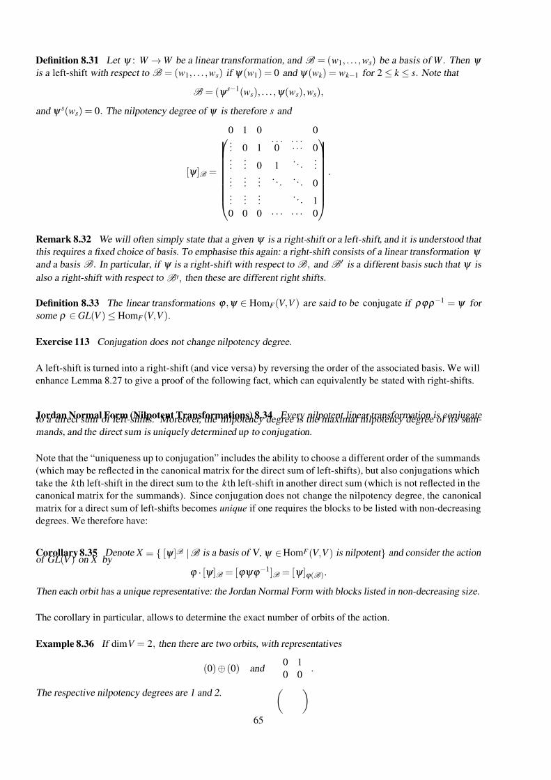
7/26/2019 MATH 2968 Algebra Advanced Notes
http://slidepdf.com/reader/full/math-2968-algebra-advanced-notes 65/110
Definition 8.31 Let ψ : W → W be a linear transformation, and B = (w1, . . . , ws) be a basis of W . Then ψ
is a left-shift with respect to B = (w1, . . . , ws) if ψ (w1) = 0 and ψ (wk ) = wk −1 for 2 ≤ k ≤ s. Note that
B = (ψ s−1(ws), . . . ,ψ (ws), ws),
and ψ s(ws) = 0. The nilpotency degree of ψ is therefore s and
[ψ ]B =
0 1 0 · · · · · ·
0... 0 1 0 · · · 0...
... 0 1 . . .
......
......
. . . . . . 0
......
... . . . 1
0 0 0 · · · · · · 0
.
Remark 8.32 We will often simply state that a given ψ is a right-shift or a left-shift, and it is understood that
this requires a fixed choice of basis. To emphasise this again: a right-shift consists of a linear transformation ψ
and a basis B . In particular, if ψ is a right-shift with respect to B , and B is a different basis such that ψ is
also a right-shift with respect to B , then these are different right shifts.
Definition 8.33 The linear transformations ϕ ,ψ ∈ HomF (V ,V ) are said to be conjugate if ρϕρ−1 = ψ for
some ρ ∈ GL(V ) ≤ HomF (V ,V ).
Exercise 113 Conjugation does not change nilpotency degree.
A left-shift is turned into a right-shift (and vice versa) by reversing the order of the associated basis. We will
enhance Lemma 8.27 to give a proof of the following fact, which can equivalently be stated with right-shifts.
Jordan Normal Form (Nilpotent Transformations) 8.34 Every nilpotent linear transformation is conjugate to a direct sum of left-shifts. Moreover, the nilpotency degree is the maximal nilpotency degree of its sum-
mands, and the direct sum is uniquely determined up to conjugation.
Note that the “uniqueness up to conjugation” includes the ability to choose a different order of the summands
(which may be reflected in the canonical matrix for the direct sum of left-shifts), but also conjugations which
take the k th left-shift in the direct sum to the k th left-shift in another direct sum (which is not reflected in the
canonical matrix for the summands). Since conjugation does not change the nilpotency degree, the canonical
matrix for a direct sum of left-shifts becomes unique if one requires the blocks to be listed with non-decreasing
degrees. We therefore have:
Corollary 8.35 Denote X = [ψ ]B |B is a basis of V, ψ ∈HomF (V ,V ) is nilpotent and consider the actionof GL(V ) on X by
ϕ · [ψ ]B = [ϕψϕ −1]B = [ψ ]ϕ (B ).
Then each orbit has a unique representative: the Jordan Normal Form with blocks listed in non-decreasing size.
The corollary in particular, allows to determine the exact number of orbits of the action.
Example 8.36 If dimV = 2, then there are two orbits, with representatives
(0) ⊕ (0) and
0 1
0 0.
The respective nilpotency degrees are 1 and 2.
65
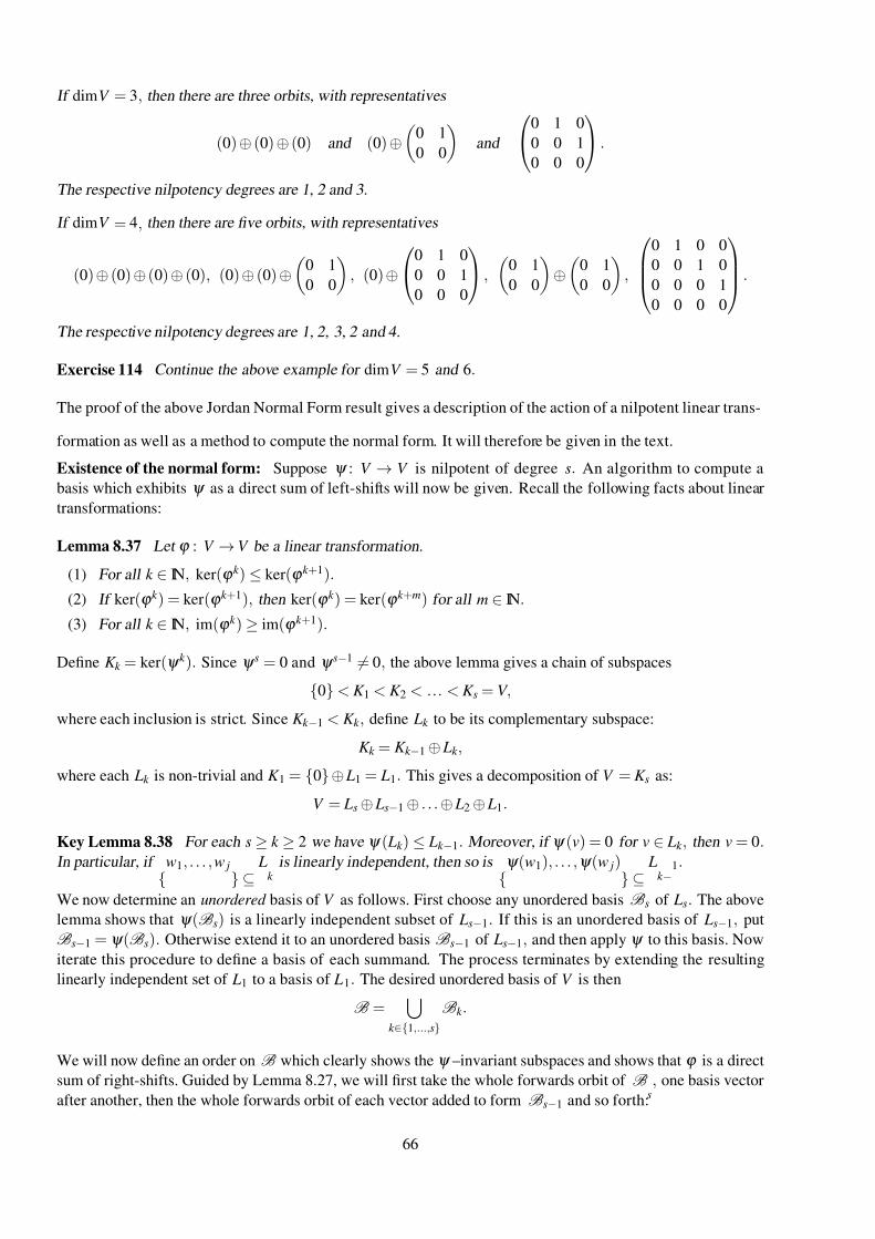
7/26/2019 MATH 2968 Algebra Advanced Notes
http://slidepdf.com/reader/full/math-2968-algebra-advanced-notes 66/110
If dimV = 3, then there are three orbits, with representatives
(0)⊕ (0) ⊕ (0) and (0) ⊕
0 1
0 0
and
0 1 0
0 0 1
0 0 0
.
The respective nilpotency degrees are 1, 2 and 3.
If dimV = 4, then there are five orbits, with representatives
(0)⊕ (0) ⊕ (0)⊕ (0), (0)⊕ (0) ⊕
0 1
0 0
, (0)⊕
0 1 0
0 0 1
0 0 0
,
0 1
0 0
⊕
0 1
0 0
,
0 1 0 0
0 0 1 0
0 0 0 1
0 0 0 0
.
The respective nilpotency degrees are 1, 2, 3, 2 and 4.
Exercise 114 Continue the above example for dimV = 5 and 6.
The proof of the above Jordan Normal Form result gives a description of the action of a nilpotent linear trans-
formation as well as a method to compute the normal form. It will therefore be given in the text.
Existence of the normal form: Suppose ψ : V → V is nilpotent of degree s. An algorithm to compute a
basis which exhibits ψ as a direct sum of left-shifts will now be given. Recall the following facts about linear
transformations:
Lemma 8.37 Let ϕ : V → V be a linear transformation.
(1) For all k ∈ IN, ker(ϕ k ) ≤ ker(ϕ k +1).
(2) If ker(ϕ k ) = ker(ϕ k +1), then ker(ϕ k ) = ker(ϕ k +m) for all m ∈ IN.
(3) For all k ∈ IN, im(ϕ k ) ≥ im(ϕ k +1).
Define K k = ker(ψ k ). Since ψ s = 0 and ψ s−1 = 0, the above lemma gives a chain of subspaces
0 < K 1 < K 2 < ... < K s = V ,
where each inclusion is strict. Since K k −1 < K k , define Lk to be its complementary subspace:
K k = K k −1 ⊕ Lk ,
where each Lk is non-trivial and K 1 = 0⊕ L1 = L1. This gives a decomposition of V = K s as:
V = Ls ⊕ Ls−1 ⊕ . . . ⊕ L2 ⊕ L1.
Key Lemma 8.38 For each s ≥ k ≥ 2 we have ψ ( Lk ) ≤ Lk −1. Moreover, if ψ (v) = 0 for v ∈ Lk , then v = 0.In particular, if
w1, . . . , w j
⊆ L
k is linearly independent, then so is
ψ (w1), . . . ,ψ (w j)
⊆ L
k −1.
We now determine an unordered basis of V as follows. First choose any unordered basis B s of Ls. The above
lemma shows that ψ (B s) is a linearly independent subset of Ls−1. If this is an unordered basis of Ls−1, put
B s−1 = ψ (B s). Otherwise extend it to an unordered basis B s−1 of Ls−1, and then apply ψ to this basis. Now
iterate this procedure to define a basis of each summand. The process terminates by extending the resulting
linearly independent set of L1 to a basis of L1. The desired unordered basis of V is then
B =
k ∈1,...,sB k .
We will now define an order on B which clearly shows the ψ –invariant subspaces and shows that ϕ is a direct
sum of right-shifts. Guided by Lemma 8.27, we will first take the whole forwards orbit of B s, one basis vector
after another, then the whole forwards orbit of each vector added to form B s−1 and so forth:
66
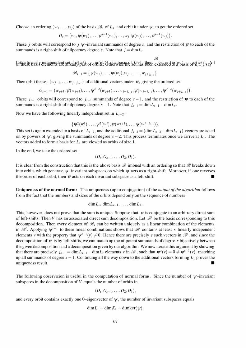
7/26/2019 MATH 2968 Algebra Advanced Notes
http://slidepdf.com/reader/full/math-2968-algebra-advanced-notes 67/110
Choose an ordering (w1, . . . , w j) of the basis B s of Ls, and orbit it under ψ , to get the ordered set
Os =
w1,ψ (w1), . . . ,ψ s−1(w1), . . . , w j,ψ (w j), . . . ,ψ s−1(w j)
.
These j orbits will correspond to j ψ –invariant summands of degree s, and the restriction of ψ to each of the
summands is a right-shift of nilpotency degree s. Note that j = dim Ls.
If the linearly independent set ψ (w1), . . . ,ψ (w j) is a basis of Ls−1, then B
s−1 = ψ (w1), . . . ,ψ (w j). Allof these basis elements are already part of orbits. Otherwise the set has been extended to a basis of Ls−1, say
B s−1 = ψ (w1), . . . ,ψ (w j), w j+1, . . . , w j+ js−1.
Then orbit the set w j+1, . . . , w j+ js−1 of additional vectors under ψ , giving the ordered set
Os−1 =
w j+1,ψ (w j+1), . . . ,ψ s−2(w j+1), . . . w j+ js−1,ψ (w j+ js−1
), . . . ,ψ s−2(w j+ js−1)
.
These js−1 orbits will correspond to js−1 summands of degree s − 1, and the restriction of ψ to each of the
summands is a right-shift of nilpotency degree s − 1. Note that js−1 = dim Ls−1 − dim Ls.
Now we have the following linearly independent set in Ls−2 :
ψ 2(w1), . . . ,ψ 2(w j),ψ (w j+1), . . . ,ψ (w j+ js−1 ).
This set is again extended to a basis of Ls−2, and the additional js−2 = (dim Ls−2 −dim Ls−1) vectors are acted
on by powers of ψ , giving the summands of degree s − 2. This process terminates once we arrive at L1. The
vectors added to form a basis for L1 are viewed as orbits of size 1.
In the end, we take the ordered set
(Os, Os−1, . . . , O2, O1).
It is clear from the construction that this is the above basis B imbued with an ordering so that B breaks down
into orbits which generate ψ –invariant subspaces on which ψ acts as a right-shift. Moreover, if one reverses
the order of each orbit, then ψ acts on each invariant subspace as a left-shift.
Uniqueness of the normal form: The uniqueness (up to conjugation) of the output of the algorithm follows
from the fact that the numbers and sizes of the orbits depend only on the sequence of numbers
dim Ls, dim Ls−1, . . . , dim L1.
This, however, does not prove that the sum is unique. Suppose that ψ is conjugate to an arbitrary direct sum
of left-shifts. Then V has an associated direct sum decomposition. Let B be the basis corresponding to this
decomposition. Then every element of B s can be written uniquely as a linear combination of the elements
in B . Applying ψ s−1 to these linear combinations shows that B contains at least s linearly independent
elements v with the property that ψ s−1(v) = 0. Hence there are precisely s such vectors in B , and since the
decomposition of ψ is by left-shifts, we can match up the nilpotent summands of degree s bijectively between
the given decomposition and a decomposition given by our algorithm. We now iterate this argument by showing
that there are precisely js−1 = dim Ls−1 − dim Ls elements v in B , such that ψ s(v) = 0 = ψ s−1(v), matching
up all summands of degree s − 1. Continuing all the way down to the additional vectors forming L1 proves the
uniqueness result.
The following observation is useful in the computation of normal forms. Since the number of ψ –invariant
subspaces in the decomposition of V equals the number of orbits in
(Os, Os−1, . . . , O2, O1),
and every orbit contains exactly one 0–eigenvector of ψ , the number of invariant subspaces equals
dim L1 = dim K 1 = dimker(ψ ).
67
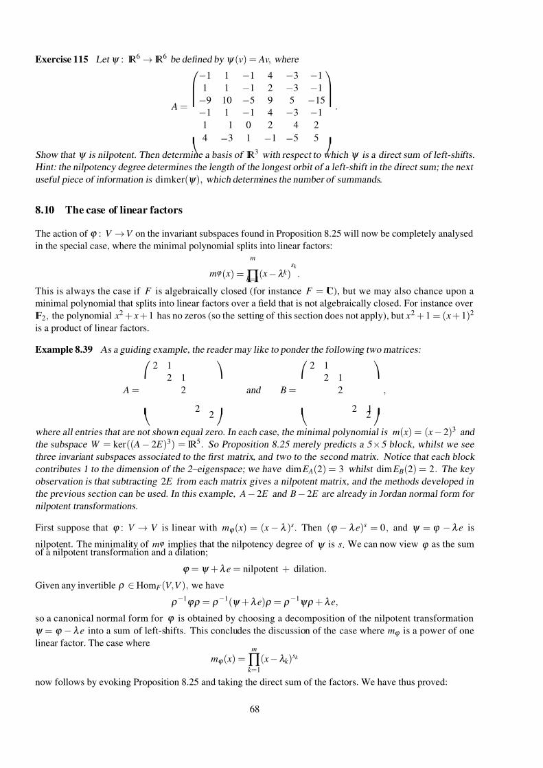
7/26/2019 MATH 2968 Algebra Advanced Notes
http://slidepdf.com/reader/full/math-2968-algebra-advanced-notes 68/110
Exercise 115 Let ψ : IR6 → IR6 be defined by ψ (v) = Av, where
A =
−1 1 −1 4 −3 −1
1 1 −1 2 −3 −1
−9 10 −5 9 5 −15
−1 1 −1 4 −3 −1
1
−1 0 2
−4 2
4 −3 1 −1 −5 5
.
Show that ψ is nilpotent. Then determine a basis of IR3 with respect to which ψ is a direct sum of left-shifts.
Hint: the nilpotency degree determines the length of the longest orbit of a left-shift in the direct sum; the next
useful piece of information is dimker(ψ ), which determines the number of summands.
8.10 The case of linear factors
The action of ϕ : V → V on the invariant subspaces found in Proposition 8.25 will now be completely analysed
in the special case, where the minimal polynomial splits into linear factors:
mϕ ( x) =
m
∏k =1( x −λ k )
sk
.
This is always the case if F is algebraically closed (for instance F = C), but we may also chance upon a
minimal polynomial that splits into linear factors over a field that is not algebraically closed. For instance over
IF2, the polynomial x2 + x + 1 has no zeros (so the setting of this section does not apply), but x2 + 1 = ( x + 1)2
is a product of linear factors.
Example 8.39 As a guiding example, the reader may like to ponder the following two matrices:
A =
2 1
2 1
2
22
and B =
2 1
2 1
2
2 12
,
where all entries that are not shown equal zero. In each case, the minimal polynomial is m( x) = ( x − 2)3 and
the subspace W = ker(( A − 2 E )3) = IR5. So Proposition 8.25 merely predicts a 5 ×5 block, whilst we see
three invariant subspaces associated to the first matrix, and two to the second matrix. Notice that each block
contributes 1 to the dimension of the 2–eigenspace; we have dim E A(2) = 3 whilst dim E B(2) = 2. The key
observation is that subtracting 2 E from each matrix gives a nilpotent matrix, and the methods developed in
the previous section can be used. In this example, A − 2 E and B − 2 E are already in Jordan normal form for
nilpotent transformations.
First suppose that ϕ : V → V is linear with mϕ ( x) = ( x − λ )s. Then (ϕ − λ e)s = 0, and ψ = ϕ −λ e is
nilpotent. The minimality of mϕ implies that the nilpotency degree of ψ is s. We can now view ϕ as the sumof a nilpotent transformation and a dilation;
ϕ = ψ +λ e = nilpotent + dilation.
Given any invertible ρ ∈ HomF (V ,V ), we have
ρ−1ϕρ = ρ−1(ψ +λ e)ρ = ρ−1ψρ +λ e,
so a canonical normal form for ϕ is obtained by choosing a decomposition of the nilpotent transformation
ψ = ϕ −λ e into a sum of left-shifts. This concludes the discussion of the case where mϕ is a power of one
linear factor. The case where
mϕ ( x) =m
∏k =1
( x −λ k )sk
now follows by evoking Proposition 8.25 and taking the direct sum of the factors. We have thus proved:
68
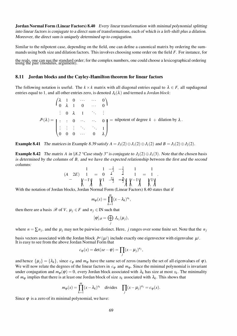
7/26/2019 MATH 2968 Algebra Advanced Notes
http://slidepdf.com/reader/full/math-2968-algebra-advanced-notes 69/110
Jordan Normal Form (Linear Factors) 8.40 Every linear transformation with minimal polynomial splitting
into linear factors is conjugate to a direct sum of transformations, each of which is a left-shift plus a dilation.
Moreover, the direct sum is uniquely determined up to conjugation.
Similar to the nilpotent case, depending on the field, one can define a canonical matrix by ordering the sum-
mands using both size and dilation factors. This involves choosing some order on the field F . For instance, for
the reals, one can use the standard order; for the complex numbers, one could choose a lexicographical orderingusing the pair (modulus, argument).
8.11 Jordan blocks and the Cayley-Hamilton theorem for linear factors
The following notation is useful. The k × k matrix with all diagonal entries equal to λ ∈ F , all supdiagonal
entries equal to 1, and all other entries zero, is denoted J k (λ ) and termed a Jordan block :
J k (λ ) =
λ 1 0 · · · · · · 0
0 λ 1 0 · · · 0... 0 λ 1
. . . ...
... ... 0 . . . . . . 0
......
... . . .
. . . 1
0 0 0 · · · 0 λ
= nilpotent of degree k + dilation by λ .
Example 8.41 The matrices in Example 8.39 satisfy A = J 3(2) ⊕ J 1(2) ⊕ J 1(2) and B = J 3(2)⊕ J 2(2).
Example 8.42 The matrix A in §8.2 “Case study 3” is conjugate to J 2(2) ⊕ J 1(3). Note that the chosen basis
is determined by the columns of B, and we have the expected relationship between the first and the second
columns:
( A−
2 E )1
1
−1 =
1 − 12
− 12
0 1
2 −1
21 − 12
− 12
1
1
−1 =
1
1
1 .
With the notation of Jordan blocks, Jordan Normal Form (Linear Factors) 8.40 states that if
mϕ ( x) =m
∏k =1
( x −λ k )sk ,
then there are a basis B of V , µ j ∈ F and n j ∈ IN such that
[ϕ ]B =
j
J n j(µ j),
where n = ∑n j, and the µ j may not be pairwise distinct. Here, j ranges over some finite set. Note that the n j
basis vectors associated with the Jordan block J n j (µ j) include exactly one eigenvector with eigenvalue µ j.It is easy to see from the above Jordan Normal Form that
cϕ ( x) = det( xe −ϕ ) =∏ j
( x −µ j)n j ,
and hence µ j = λ k , since cϕ and mϕ have the same set of zeros (namely the set of all eigenvalues of ϕ ).
We will now relate the degrees of the linear factors in cϕ and mϕ . Since the minimal polynomial is invariant
under conjugation and mϕ (ϕ ) = 0, every Jordan block associated with λ k has size at most sk . The minimality
of mϕ implies that there is at least one Jordan block of size sk associated with λ k . This shows that
mϕ ( x) =m
∏k =1
( x −λ k )sk divides ∏
j
( x −µ j)n j = cϕ ( x).
Since ϕ is a zero of its minimal polynomial, we have:
69
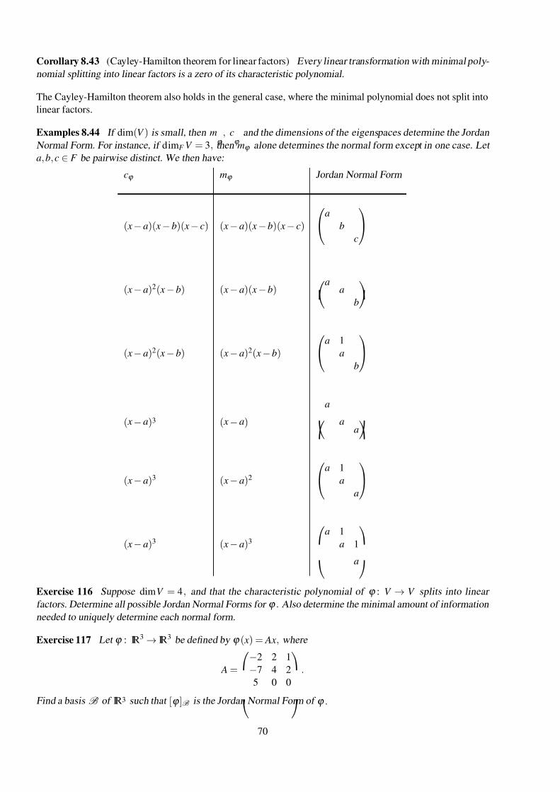
7/26/2019 MATH 2968 Algebra Advanced Notes
http://slidepdf.com/reader/full/math-2968-algebra-advanced-notes 70/110
Corollary 8.43 (Cayley-Hamilton theorem for linear factors) Every linear transformation with minimal poly-
nomial splitting into linear factors is a zero of its characteristic polynomial.
The Cayley-Hamilton theorem also holds in the general case, where the minimal polynomial does not split into
linear factors.
Examples 8.44 If dim(V ) is small, then mϕ
, cϕ
and the dimensions of the eigenspaces determine the Jordan
Normal Form. For instance, if dimF V = 3, then mϕ alone determines the normal form except in one case. Let
a, b, c ∈ F be pairwise distinct. We then have:
cϕ mϕ Jordan Normal Form
( x − a)( x − b)( x − c) ( x − a)( x −b)( x − c)
a
b
c
( x − a)2( x − b) ( x − a)( x −b)a
a
b
( x − a)2( x − b) ( x − a)2( x −b)
a 1
a
b
( x − a)3 ( x − a) a
aa
( x − a)3 ( x − a)2
a 1
a
a
( x − a)3 ( x − a)3
a 1
a 1
a
Exercise 116 Suppose dimV = 4, and that the characteristic polynomial of ϕ : V → V splits into linear
factors. Determine all possible Jordan Normal Forms for ϕ . Also determine the minimal amount of information
needed to uniquely determine each normal form.
Exercise 117 Let ϕ : IR3 → IR3 be defined by ϕ ( x) = Ax, where
A =
−2 2 1
−7 4 2
5 0 0
.
Find a basis B of IR3 such that [ϕ ]B is the Jordan Normal Form of ϕ .
70
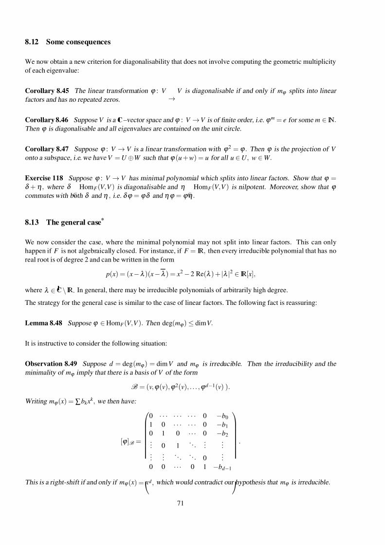
7/26/2019 MATH 2968 Algebra Advanced Notes
http://slidepdf.com/reader/full/math-2968-algebra-advanced-notes 71/110
8.12 Some consequences
We now obtain a new criterion for diagonalisability that does not involve computing the geometric multiplicity
of each eigenvalue:
Corollary 8.45 The linear transformation ϕ : V →
V is diagonalisable if and only if mϕ splits into linear
factors and has no repeated zeros.
Corollary 8.46 Suppose V is a C –vector space and ϕ : V → V is of finite order, i.e. ϕ m = e for some m ∈ IN.Then ϕ is diagonalisable and all eigenvalues are contained on the unit circle.
Corollary 8.47 Suppose ϕ : V → V is a linear transformation with ϕ 2 = ϕ . Then ϕ is the projection of V
onto a subspace, i.e. we have V = U ⊕W such that ϕ (u + w) = u for all u ∈ U , w ∈ W .
Exercise 118 Suppose ϕ : V → V has minimal polynomial which splits into linear factors. Show that ϕ =δ + η , where δ
∈ HomF (V ,V ) is diagonalisable and η
∈ HomF (V ,V ) is nilpotent. Moreover, show that ϕ
commutes with both δ and η , i.e. δ ϕ = ϕδ and ηϕ = ϕη .
8.13 The general case*
We now consider the case, where the minimal polynomial may not split into linear factors. This can only
happen if F is not algebraically closed. For instance, if F = IR, then every irreducible polynomial that has no
real root is of degree 2 and can be written in the form
p( x) = ( x −λ )( x −λ ) = x2 − 2 Re(λ ) + |λ |2 ∈ IR[ x],
where λ ∈ C \ IR. In general, there may be irreducible polynomials of arbitrarily high degree.
The strategy for the general case is similar to the case of linear factors. The following fact is reassuring:
Lemma 8.48 Suppose ϕ ∈ HomF (V ,V ). Then deg(mϕ ) ≤ dimV .
It is instructive to consider the following situation:
Observation 8.49 Suppose d = deg(mϕ ) = dim V and mϕ is irreducible. Then the irreducibility and the
minimality of mϕ imply that there is a basis of V of the form
B = (v,ϕ (v),ϕ 2(v), . . . ,ϕ d −1(v) ).
Writing mϕ ( x) = ∑bk xk , we then have:
[ϕ ]B =
0 · · · · · · · · · 0 −b0
1 0 · · · · · · 0 −b1
0 1 0 · · · 0 −b2
... 0 1 . . .
......
......
. . . . . . 0
...
0 0 · · · 0 1 −bd −1
.
This is a right-shift if and only if mϕ ( x) = xd , which would contradict our hypothesis that mϕ is irreducible.
71
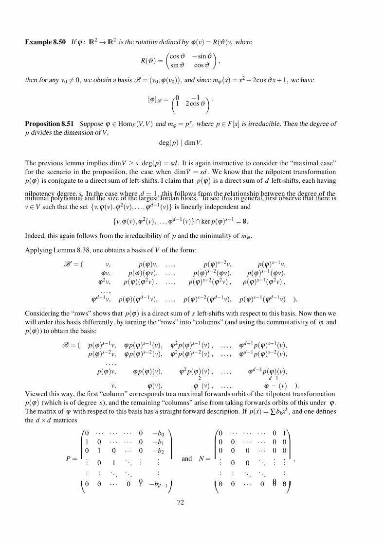
7/26/2019 MATH 2968 Algebra Advanced Notes
http://slidepdf.com/reader/full/math-2968-algebra-advanced-notes 72/110
Example 8.50 If ϕ : IR2 → IR2 is the rotation defined by ϕ (v) = R(ϑ )v, where
R(ϑ ) =
cosϑ −sinϑ
sinϑ cosϑ
,
then for any v0 = 0, we obtain a basis B = (v0,ϕ (v0)), and since mϕ ( x) = x2 − 2cosϑ x + 1, we have
[ϕ ]B =0 −1
1 2 cosϑ
.
Proposition 8.51 Suppose ϕ ∈ HomF (V ,V ) and mϕ = ps, where p ∈ F [ x] is irreducible. Then the degree of
p divides the dimension of V ,
deg( p) | dimV .
The previous lemma implies dimV ≥ s deg( p) = sd . It is again instructive to consider the “maximal case”
for the scenario in the proposition, the case when dimV = sd . We know that the nilpotent transformation
p(ϕ ) is conjugate to a direct sum of left-shifts. I claim that p(ϕ ) is a direct sum of d left-shifts, each having
nilpotency degree s. In the case where d = 1, this follows from the relationship between the degree of theminimal polynomial and the size of the largest Jordan block. To see this in general, first observe that there is
v ∈ V such that the set v,ϕ (v),ϕ 2(v), . . . ,ϕ d −1(v) is linearly independent and
v,ϕ (v),ϕ 2(v), . . . ,ϕ d −1(v)∩ ker p(ϕ )s−1 = / 0.
Indeed, this again follows from the irreducibility of p and the minimality of mϕ .
Applying Lemma 8.38, one obtains a basis of V of the form:
B = ( v, p(ϕ )v, . . . , p(ϕ )s−2v, p(ϕ )s−1v,
ϕ v, p(ϕ )(ϕ v), . . . , p(ϕ )s−2(ϕ v), p(ϕ )s−1(ϕ v),ϕ 2v, p(ϕ )(ϕ 2v) , . . . , p(ϕ )s−2(ϕ 2v) , p(ϕ )s−1(ϕ 2v) ,
. . . ,
ϕ d −1v, p(ϕ )(ϕ d −1v), . . . , p(ϕ )s−2(ϕ d −1v), p(ϕ )s−1(ϕ d −1v) ).
Considering the “rows” shows that p(ϕ ) is a direct sum of s left-shifts with respect to this basis. Now then we
will order this basis differently, by turning the “rows” into “columns” (and using the commutativity of ϕ and
p(ϕ )) to obtain the basis:
B = ( p(ϕ )s−1v, ϕ p(ϕ )s−1(v), ϕ 2 p(ϕ )s−1(v) , . . . , ϕ d −1 p(ϕ )s−1(v),
p(ϕ )s−2v, ϕ p(ϕ )s−2(v), ϕ 2 p(ϕ )s−2(v) , . . . , ϕ d −1 p(ϕ )s−2(v),
. . . ,
p(ϕ )v, ϕ p(ϕ )(v), ϕ 2 p(ϕ )(v) , . . . , ϕ d −1 p(ϕ )(v),
v, ϕ (v), ϕ 2
(v) , . . . , ϕ d
−1
(v) ).
Viewed this way, the first “column” corresponds to a maximal forwards orbit of the nilpotent transformation
p(ϕ ) (which is of degree s), and the remaining “columns” arise from taking forwards orbits of this under ϕ .The matrix of ϕ with respect to this basis has a straight forward description. If p( x) = ∑bk x
k , and one defines
the d × d matrices
P =
0 · · · · · · · · · 0 −b0
1 0 · · · · · · 0 −b1
0 1 0 · · · 0 −b2
... 0 1 . . .
......
..
.
..
.
. . . . . .
0
..
.0 0 · · · 0 1 −bd −1
and N =
0 · · · · · · · · · 0 1
0 0 · · · · · · 0 0
0 0 0 · · · 0 0... 0 0
. . . ...
.....
.
..
.
. . . . . .
0
..
.0 0 · · · 0 0 0
,
72
7/26/2019 MATH 2968 Algebra Advanced Notes
http://slidepdf.com/reader/full/math-2968-algebra-advanced-notes 73/110
then we have the (sd ) × (sd ) matrix
[ϕ ]B =
P N 0 ·· · · · · 0
0 P N 0 · · · 0... 0 P N 0
......
... 0 . . .
. . . 0
... ... 0 P N
0 0 0 · · · 0 P
= block of size sd associated with p.
Notice that
[ϕ ]B = nilpotent matrix + block-diagonal matrix.
If d = 1, then p( x) = x+b0 and this reduces to P = (−b0) and N = (1), hence giving the Jordan block J s(−b0).As in the case for linear factors, if sd < dimV , then there is at least one block of size sd , and additional blocks
of the above form, but with respective sizes a multiple of d that is possibly smaller than sd .
Theorem 8.52 (Jordan normal form) Every linear transformation is conjugate to a direct sum of transforma-
tions, each of which has a canonical matrix as described above. The direct sum is unique up to conjugation.
The following result shows that the minimal polynomial determines the characteristic polynomial if the former
has a unique irreducible factor. This can be verified directly using the matrices derived above, or be proved
independently.
Lemma 8.53 If mϕ = ps, where p ∈ F [ x] is irreducible, then cϕ = pn/d , where n = dimV and d = deg( p).
Putting the above results together using the natural direct sum, gives:
Proposition 8.54 Suppose mϕ =m
∏k =1
( pk )sk , where sk
∈IN, each pk
∈F [ x] is irreducible, monic and pk
= p j
for all k = j. Let W k = ker(( pk (ϕ ))sk ), nk = dim W k and d k = deg( pk ). Then d k divides nk for each k , and
cϕ =m
∏k =1
( pk )nk /d k .
Corollary 8.55 (Cayley-Hamilton theorem) Let ϕ ∈ HomF (V ,V ). Then cϕ (ϕ ) = 0 ∈ HomF (V ,V ).
73
7/26/2019 MATH 2968 Algebra Advanced Notes
http://slidepdf.com/reader/full/math-2968-algebra-advanced-notes 74/110
9 Group presentations*
Group presentations have been used informally in these notes. This section gives a brief introduction to free
groups and group presentations. Whilst the statements of the results and the methods are intuitively clear, the
proofs are omitted because an algebraic treatment would be rather long, and the modern treatment requires
ideas from algebraic topology. The interested reader is referred to Marc Lackenby’s excellent set of notes [17].
9.1 Free groups*
For any set S , we will define the free group on S , denoted F (S ). I’ll start with an example. If S = a, b, then
S is our alphabet with which we write words such as aabab but also aba−1. The words are viewed as elements
of F (S ) with the only caveat that the empty word is going to be the identity e ∈ F (S ) and that
e = aa−1 = a−1a = bb−1 = b−1b,
and hence, for example, aa−1
b = b. The (undirected) Cayley graph constructed from this particular generatingset a, b is the four-valent tree (there are precisely four edges incident with each vertex). The fact that we
have to declare certain words, such as aa−1b and b, to be the same element of F (S ) means that elements really
are equivalence classes of words. I will define free groups.
Let S be a set, called the alphabet , and construct the set S −1 = s−1 | s ∈ S . We therefore have a bijection
S → S −1 and require S ∩ S −1 = / 0 and e /∈ S ∪ S −1. For s−1 ∈ S −1, we write (s−1)−1 = s.
A word w in the alphabet S is a finite sequence x1, x2, . . . , xm with each xk ∈ S ∪ S −1. We will write w = x1 x2 . . . xm. The empty sequence is also allowed and denoted w = e. The concatenation of words x1 x2 . . . xm and
y1 y2 . . . yn is the word x1 x2 . . . xm y1 y2 . . . yn.
The word w1 is an elementary contraction of the word w2 if there are words v1 and v2 and s ∈ S ∪ S −1
suchthat w2 = v1s−1sv2 and w1 = v1v2. We also say that w2 is an elementary expansion of w1.
Two words are equivalent if one can be obtained from the other by a finite sequence of elementary contractions
or expansions. This is an equivalence relation on the set of all words, and we denote the equivalence class of w
by [w].
Definition 9.1 The free group on S , denoted F (S ), is the set of all equivalence classes of words in the alphabet
S , where the group operation is given by concatenation of representatives:
[w1] [w2] = [w1w2].
It is a pleasant exercise to check that this multiplication is indeed well-defined and turns F (S ) into a group with
identity element the equivalence class of the empty word.
It is also easy to decide when two elements in F (S ) are equal. Given a word w, repeatedly perform elementary
contractions until it is in reduced form, where no elementary contraction is possible. Any equivalence class of
words contains a unique word in reduced form. Hence [w1] = [w2] if and only if the reduced forms of w1 and
w2 are equal.
There is a natural inclusion ι : S → F (S ) given by s → [s]. It was shown in Exercise 32 that a homomorphism is
uniquely determined by its action on the generators. Since free groups have no relations between the generators,
one can map them to whichever elements one likes. This is the universal property of free groups:
74
7/26/2019 MATH 2968 Algebra Advanced Notes
http://slidepdf.com/reader/full/math-2968-algebra-advanced-notes 75/110
Theorem 9.2 (Universal property of free groups) Suppose S is a set, G is a group and f : S → G is any
function. There there is a unique homomorphism ϕ : F (S ) → G such that the following diagram commutes:
S f G
ϕ
F (S )
ι
The size of S is called the rank of F (S ). It follows from the universal property that if |S | = |S |, then F (S ) ∼=F (S ) by choosing a bijection between S and S . In particular, for each n ∈ IN there is (up to isomorphism)
precisely one free group of rank n. This is denoted IFn.
Up until the 1980’s free groups and their subgroups were studied using combinatorial methods, such as the
so-called Schreier rewriting method and Nielsen transformations, and many proofs in this area were long and
complicated. The field was revolutionised by Stallings [20], who introduced a topological approach, mainly
using covering space theory and graph-theoretic arguments. For instance, Stallings gave an elegant and fairlysimple proof of the following theorem.
Theorem 9.3 (Nielsen-Schreier) Every subgroup of a finitely generated free group is free.
It follows from the universal property of free groups that for every group, there is a free group that surjects onto
it. Indeed, given the group G, construct F (G) and apply Theorem 9.2 to the identity map G → G. Then the
homomorphism F (G) → G is clearly surjective. This is, of course, highly inefficient. For instance, applied to
the cyclic group C n this gives an epimorphism IFn →C n, but clearly there also is an epimorphism ZZ ∼= IF1 →C n.
9.2 Group presentations*
I now want to make precise the idea of writing IF1 = a, IF2 = a, b, and introducing extra relations between
the generators that allow statements such as:
C n ∼= a | an = 1;
Dn ∼= a, b | an = e, b2 = e, bab = a−1.
This should be contrasted with the earlier notation. We wrote H = S ≤ G, where S is a set of elements from
G, and S is the set of all elements of G that are finite products of elements from S and S −1. In that setting,
we know what the elements and the relationships between them are, because G is a given group. Hence if one
chooses an appropriate rotation σ ∈ Dn and an appropriate reflection τ ∈ Dn, then Dn = σ ,τ , and we have,amongst others, the equalities
σ n = e, τ 2 = e, τστ = σ −1.
We now want to make precise what it means to define a group by an expression such as
a, b | an = e, b2 = e, bab = a−1,
where all identities involving a and b (and e ) are supposed to follow from elementary expansions and contrac-
tions plus the three given identities.
Let G be a group and B ⊆ G be a subset. The normal closure of B, denoted B is the intersection of all
normal subgroups of G containing B. This is again a normal subgroup, and hence the smallest normal subgroup
of G containing B. The elements of B have a very explicit form:
75
7/26/2019 MATH 2968 Algebra Advanced Notes
http://slidepdf.com/reader/full/math-2968-algebra-advanced-notes 76/110
Lemma 9.4 (Normal form lemma) Every element of B is of the form
n
∏k =1
g−1k b
ε k
k gk ,
where k ∈ 0∪ IN, gk ∈ G and ε k ∈ ±1 for all k .
Definition 9.5 (Group presentation) Let S be a set and R ⊆ F (S ). The group with presentation S | R isdefined to be the quotient group F (S )/ R.
For the free group or rank n, we will write IFn = a1, . . . , an in place of a1, . . . , an | e.
Remark 9.6 The elements of S are called the generators and the elements of R are called relators. Instead of
an expression such as
a, b | an, b2 , abab,
as dictated by the definition, we will often write relations in place of relators:
a, b
|an = e, b2 = e, bab = a−1
.
Any way to transform a relation into a relator gives the same group by the normal form lemma. We will use
words in the alphabet S to represent elements of S | R; however, one should keep in mind that the elements
of S | R really are cosets of R represented by equivalence classes of words.
We call S | R a presentation of the group F (S )/ R. If both S and R are finite, the presentation is said to be
finite. The group G is finitely presented if it has a finite presentation. The next set of results says that we can
work with presentations in the way that is suggested by the notation.
Lemma 9.7 Let G = S | R. Then two words in the alphabet S represent the same element of G if and only
if they differ by a finite sequence of
(1) elementary contractions or expansions, or
(2) insertions of relators or their inverses.
Lemma 9.8 Suppose G = S | R and H is a group. We know that any function f : S → H induces a ho-
momorphism ϕ : F (S ) → H . Then ϕ descends to a homomorphism G → H if and only if ϕ (r ) = e H for all
r ∈ R.
Exercise 119 Let IF2 = a, b and ϕ : IF2 → ZZ be the homomorphism defined by ϕ (a) = 1 = ϕ (b). Show
that the kernel of ϕ is not finitely generated.
The following result sometimes helps to simplify a presentation or (if you are lucky) to tell whether two groupsare isomorphic:
Theorem 9.9 (Tietze) Any two finite presentations of a group G are convertible into each other by a finite
sequence of the following Tietze transformations:
(T1) Re-order the generators or relators.
(T2) Add or remove the relator e.
(T3) Perform an elementary expansion or contraction to a relator.
(T4) Insert (resp. remove) a relator or its inverse into (resp. from) one of the other relators.
(T5) Take a word w in the generators, and add a new generator s to S and a new relator ws−1 to R.Or perform the reverse of this operation (if s ∈ S appears in precisely one relator).
76
7/26/2019 MATH 2968 Algebra Advanced Notes
http://slidepdf.com/reader/full/math-2968-algebra-advanced-notes 77/110
9.3 Push-outs, free products, amalgamated products and HNN extensions*
At the start of the previous section, I constructed an epimorphism F (G) → G. Denote R(G) the kernel of this
epimorphism. Then the first isomorphism theorem implies that G is isomorphic to F (G)/ R(G) and hence has
the canonical presentation G | R(G). This presentation is useful for some constructions, such as the following.
Definition 9.10 (Push-out) Let G0, G1 and G2 be groups and ϕ 1 : G0 → G1 and ϕ 2 : G0 → G2 be homomor- phisms. Let S 1 | R1 and S 2 | R2 be the canonical presentations of G1 and G2 respectively, where S 1 ∩S 2 = / 0.The the push-out G1 ∗G0
G2 of
G1 ϕ 1
G0
ϕ 2 G2
is the group
S 1 ∪ S 2 | R1 ∪ R2 ∪ϕ 1(g) = ϕ 2(g) | g ∈ G0 .
Note that we have written relations ϕ 1(g) =ϕ 2(g) instead of relators ϕ 1(g)ϕ 2(g−1). Because the canonical pre-
sentation were used, the push-out is independent of presentation, but it does depend (even though the notation
G1 ∗G0 G2 doesn’t suggest it) on the homomorphisms ϕ 1 and ϕ 2. Here is one way to compute a push-out:
Lemma 9.11 Let G0, G1 and G2 be groups and ϕ 1 : G0 → G1 and ϕ 2 : G0 → G2 be homomorphisms. Let
S 1 | R1 and S 2 | R2 be any presentations of G1 and G2 respectively, where S 1 ∩ S 2 = / 0. Then the push-out
is isomorphic with
S 1 ∪ S 2 | R1 ∪ R2 ∪ϕ 1(g) = ϕ 2(g) | g ∈ G0 .
Moreover, if G0 has generating set S 0, then the push-out is isomorphic with
S 1 ∪ S 2 | R1 ∪ R2 ∪ϕ 1(g) = ϕ 2(g) | g ∈ S 0 .
Definition 9.12 (Free product) If G0 is the trivial group, then the push-out depends only on G1 and G2. In
this case, it is written G1 ∗ G2 and called the free product of G1 and G2.
Example 9.13 (Modular group) The group PSL2(ZZ) = SL2(ZZ)/± E is called the Modular group. It isgenerated by the images of
0 −1
1 0
and
1 −1
1 0
.
These elements have orders 4 and 6 respectively in SL2(ZZ), and orders 2 and 3 in PSL2(ZZ). Their product is
an element of infinite order; and in fact:
PSL2(ZZ) ∼= C 2 ∗C 3.
Exercise 120 The free product ZZ ∗ZZ is isomorphic with IF2.
Exercise 121 Show that the free product is an associative and commutative product of groups (up to isomor-
phism).
Exercise 122 Show that IFn ∼= ZZ ∗ . . .∗ ZZ
n times
Definition 9.14 (Amalgamated free product) If both ϕ 1 : G0 → G1 and ϕ 2 : G0 → G2 are monomorphisms,
then G1 ∗G0 G2 is called the amalgamated free product of G1 and G2 along G0.
In an amalgamated free product, one glues the groups G1 and G2 together along isomorphic subgroups, hence
the name. The product, again, depends on the chosen monomorphisms, which is again not reflected in the
notation.
I conclude with an Australian construction, invented in Canberra by Graham Higman, Bernhard Neumann and
Hanna Neumann, in which two subgroups of a group are glued together in a larger group.
77
7/26/2019 MATH 2968 Algebra Advanced Notes
http://slidepdf.com/reader/full/math-2968-algebra-advanced-notes 78/110
Definition 9.15 (HNN extension) Let G = S | R, and let ϕ : G1 → G2 be an isomorphism between sub-
groups G1, G2 ≤ G. Let t be a new letter not in the alphabet S , and define
G∗ϕ = S , t | R ∪t −1gt = ϕ (g) | g ∈ G1 .
This is called the HNN extension of G relative to ϕ , G is called the base group, G1 and G2 are the associated
subgroups, and t is the stable letter.
One can show that the natural homomorphism G → G∗ϕ is injective, hence G∗ϕ really is an extension of G. It
is possible to have G1 = G, and if G1 = G = G2, then G∗ϕ contains a subgroup isomorphic with IF2.
78
7/26/2019 MATH 2968 Algebra Advanced Notes
http://slidepdf.com/reader/full/math-2968-algebra-advanced-notes 79/110
10 Proofs
10.1 Proofs of results in §1
Lemma 1.16 S is a subgroup of G , called the subgroup generated by S .
Proof The product of two finite products of elements in S ∪S −1 is again a finite product of elements in S ∪S −1.This shows that S is closed under multiplication. If a1a2 · · ·an is a finite product of elements in S ∪S −1, then
so is (a1a2 · · ·an)−1 = a−1n · · ·a−1
2 a−11 . Hence S is closed under inversion.
Lemma 1.19 Let G be a group and g ∈ G.
(1) If o(g) = ∞, then gn = gm only if m = n.
(2) If o(g) < ∞, then gn = gm if and only if m ≡ n mod o(g). In particular, o(g) = |g|.
Proof Let g ∈ G and suppose that gn = gm for some n = m. Then gn−m = gng−m = gn(gm)−1 = e, and hence
some non-zero power of g is the identity. In particular, o(g) < ∞. This proves the first part. To complete
the proof of the second part, simplify notation by writing o = o(g). Using division with remainder, write
(n − m) = qo + r with q, r ∈ ZZ and 0 ≤ r < o. Then:
gr = gn−m−qo = gn−mg−oq = e(go)−q = e−q = e.
Now 0 ≤ r < o and o = o(g), which implies that r = 0. Whence (n − m) = qo and so m ≡ n mod o(g). This
shows the forward implication. Conversely, if o(g) < ∞ and m ≡ n mod o(g), then gn = gm.
Lemma 1.20 Every subgroup of a cyclic group is cyclic.
Proof Suppose G = g is a cyclic group and let H be a subgroup of G. If H = e, then H ≤ G. Hence
suppose that H contains a non-trivial element. Since every element of G is a power of g, the same is true for H . Let gk be the smallest positive power of g that gives a non-trivial element of H . I claim that H = gk .
Suppose that gn ∈ H . Then n ≥ k , and one can use the Euclidean algorithm to write n = qk + r , where q, r ∈ ZZ
and 0 ≤ r < k . Since gk ∈ H , we have g−qk = (gk )−q ∈ H , and so gr = gn−qk = gng−qk ∈ H . Now 0 ≤ r < k ,and k is the smallest positive power of g that lies in H . Hence r = 0 and so gn = ggk = (gk )q. This shows that
every element of H is a power of gk , and hence H = gk is cyclic.
79
7/26/2019 MATH 2968 Algebra Advanced Notes
http://slidepdf.com/reader/full/math-2968-algebra-advanced-notes 80/110
10.2 Proofs of results in §2
Lemma 2.3 If H ≤ G, then an equivalence relation is defined on G by g ∼ h if and only if h−1g ∈ H .Moreover, the equivalence classes are the left cosets gH of H . Whence there is a partition of G of the form
G = j∈ J
g j H .
Moreover, the function aH → bH defined by ha → hb for h ∈ H is a bijection between aH and bH .
Proof I first give a different description of the relation, namely a−1b ∈ H if and only if aH = bH . It then
suffices to show that the cosets of H form a partition of G.
If a−1b ∈ H , then there is h ∈ H such that a−1b = h and hence b = ah ∈ aH . So if k ∈ H , then bk = (ah)k =a(hk ) ∈ aH . This shows that bH ⊆ aH . To obtain the reverse inclusion notice that if a−1b ∈ H , then also
b−1a = (a−1b)−1 ∈ H . So reversing the roles of a and b in the previous argument gives aH ⊆ bH , and hence
bH = aH . This shows that a−1b ∈ H implies aH = bH . Conversely, if aH = bH , then there is h ∈ H such that
ah = be and so a−1b = a−1be = h ∈ H .
I now show that the cosets partition G. Since g ∈ gH , it follows that every element lies in some coset. Now
suppose g ∈
aH ∩
bH .
Then there are h1,
h2 ∈
H such that ah1 =
g =
bh2.
But then g−
1a =
h−
1
1 ∈ H and
g−1b = h−12 ∈ H . By the above, aH = gH = bH . It follows that if aH ∩ bH = / 0, then aH = bH . Hence the
cosets form a partition, and therefore g ∼ h is an equivalence relation.
Last, consider the function aH → bH defined by ha → hb. This is well-defined since each element of aH can
be written uniquely in the form ah with h ∈ H . It is a bijection since it has the inverse map bH → aH given by
hb → ha.
Lagrange’s Theorem 2.9 Suppose G is a finite group and H ≤ G. Then | H | divides |G| and
|G| = |G : H | | H |.In particular, if g ∈ G, then the order of g divides |G|.
Proof Lemma 2.3 shows that the cosets of H form a partition of G, and each coset has the same number of elements as H . Whence
|G| = |G : H | | H |.The second part follows since g is a subgroup of order o(g).
Corollary 2.10 If G is a finite group of order n = |G|, then gn = e for every g ∈ G
Proof Lagrange’s theorem shows that o = o(g) divides |G| = n, so we can write n = mo for some m ∈ IN.Whence gn = gmo = (go)m = em = e.
Theorem 2.11 (Fermat’s little theorem) Let p be a prime number. If a is any integer which is not a multiple
of p, then
a p−1 ≡ 1 mod p.
Proof If p is a prime number, then the non-zero elements of ZZ p form a group under multiplication, denoted
ZZ× p . The order of this group is p−1. Now if a is any integer which is not a multiple of p, then [a] = [0] ∈ ZZ p
and hence [a] ∈ ZZ× p . The previous corollary implies that [a p−1] = [a] p−1 = [1] ∈ ZZ×
p . Whence a p−1 ≡ 1
mod p.
Theorem 2.12 Let p be a prime number. Then every group of order p is cyclic.
Proof Let G be a group of oder p and let g be a non-trivial element of G. Then g is a non-trivial subgroup
of G and by Lagrange’s theorem its oder divides |G| = p. But the only non-trivial divisor of p is p, and hence
|g| = |G|. This forces g = G.
80
7/26/2019 MATH 2968 Algebra Advanced Notes
http://slidepdf.com/reader/full/math-2968-algebra-advanced-notes 81/110
10.3 Proofs of results in §3
Lemma 3.8 Let G and H be groups and suppose ϕ : G → H is a homomorphism. Then ϕ is injective if and
only if ker(ϕ ) = eG.
Proof Suppose that ϕ is injective. Then at most one element of G is mapped to e H . We know that ϕ (eG) = e H ,and hence ker(ϕ ) = eG.
For the converse, assume ker(ϕ ) = eG. Suppose ϕ (a) = ϕ (b) for some a, b ∈ G. Then
ϕ (ab−1) = ϕ (a)ϕ (b−1) = ϕ (a)(ϕ (b))−1 = ϕ (b)(ϕ (b))−1 = e H .
Hence ab−1 ∈ ker(ϕ ) = eG, and so ab−1 = eG. Multiplying by b from the right gives a = b. So ϕ is
injective.
Lemma 3.10 Let G and H be groups and suppose ϕ : G → H is a homomorphism. Then ker(ϕ )G.
Proof Let k ∈ ker(ϕ ) and g ∈ G. Then
ϕ (g−1kg) = ϕ (g−1)ϕ (k )ϕ (g) = (ϕ (g))−1e H ϕ (g) = (ϕ (g))−1ϕ (g) = e H .
Hence g−1kg ∈ ker(ϕ ). It follows from the definition that ker(ϕ )G.
Lemma 3.11 Suppose G is a group and H ≤ G. The following are equivalent:
(1) H G
(2) For all g ∈ G we have gH = Hg.
(3) For all g ∈ G we have g−1 Hg = H .
Proof (1) =⇒ (2): Let k ∈ Hg. Then k = hg for some h ∈ H . This gives k = hg = (gg−1)hg = g(g−1hg) ∈ gH ,since g−1hg ∈ H because H is normal. This shows that Hg ⊆ gH . The reverse inclusion is similar: Let
k ∈ gH . Then k = gh for some h ∈ H . This gives k = gh = gh(g−1g) = (ghg−1)g = ((g−1)−1hg−1)g ∈ Hg
since (g−1)−1hg−1 ∈ H because H is normal. Hence gH ⊆ Hg. Combining the two inclusions gives gH = Hg.
(2) =⇒ (3): g−1 Hg = g−1( Hg) = g−1(gH ) = g−1gH = eH = H .
(3) =⇒ (1): This follows directly from the definition.
Lemma 3.13 Suppose N G. Then (gN )(hN ) = (gh) N .
Proof Since N is normal, we have (gN )(hN ) = g( Nh) N = g(hN ) N = ghNN . Since N is a subgroup, closure
under multiplication implies N N ⊆ N , and since e ∈ N , we have N ⊆ NN . Hence N N = N , giving (gN )(hN ) =ghNN = ghN .
Proposition 3.14 (Quotient group) Suppose N G. Consider the set of all left cosets of N , written
G/ N = gN | g ∈ G.
Define the operation
gN hN = (gh) N .
Then this is well-defined and turns G/ N into a group with the identity element N . Moreover, the map g
→gN
defines an epimorphism G → G/ N with kernel equal to N .
81
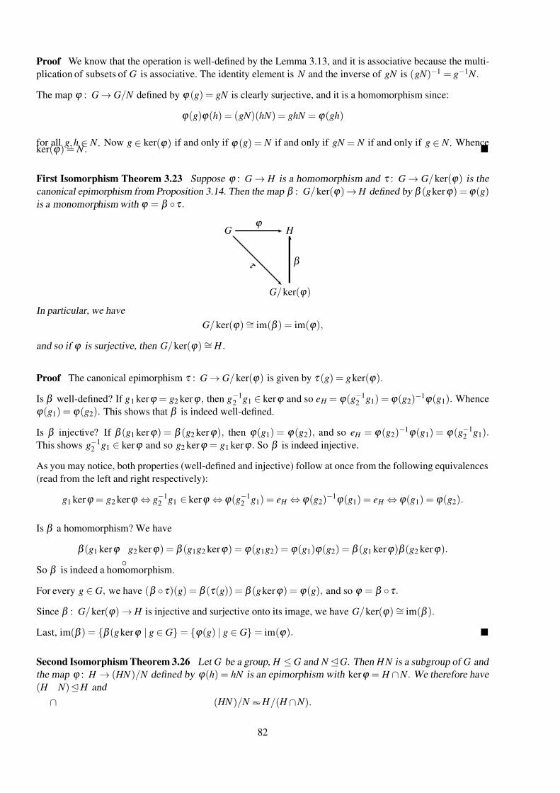
7/26/2019 MATH 2968 Algebra Advanced Notes
http://slidepdf.com/reader/full/math-2968-algebra-advanced-notes 82/110
Proof We know that the operation is well-defined by the Lemma 3.13, and it is associative because the multi-
plication of subsets of G is associative. The identity element is N and the inverse of gN is (gN )−1 = g−1 N .
The map ϕ : G → G/ N defined by ϕ (g) = gN is clearly surjective, and it is a homomorphism since:
ϕ (g)ϕ (h) = (gN )(hN ) = ghN = ϕ (gh)
for all g, h ∈ N . Now g ∈ ker(ϕ ) if and only if ϕ (g) = N if and only if gN = N if and only if g ∈ N . Whenceker(ϕ ) = N .
First Isomorphism Theorem 3.23 Suppose ϕ : G → H is a homomorphism and τ : G → G/ ker(ϕ ) is the
canonical epimorphism from Proposition 3.14. Then the map β : G/ ker(ϕ ) → H defined by β (g kerϕ ) =ϕ (g)is a monomorphism with ϕ = β τ .
Gϕ H
τ
G/ ker(ϕ )
β
In particular, we have
G/ ker(ϕ ) ∼= im(β ) = im(ϕ ),
and so if ϕ is surjective, then G/ ker(ϕ ) ∼= H .
Proof The canonical epimorphism τ : G → G/ ker(ϕ ) is given by τ (g) = g ker(ϕ ).
Is β well-defined? If g1 kerϕ = g2 kerϕ , then g−12 g1 ∈ kerϕ and so e H = ϕ (g−1
2 g1) = ϕ (g2)−1ϕ (g1). Whence
ϕ (g1) = ϕ (g2). This shows that β is indeed well-defined.
Is β injective? If β (g1 kerϕ ) = β (g2 kerϕ ), then ϕ (g1) = ϕ (g2), and so e H = ϕ (g2)−1ϕ (g1) = ϕ (g−12 g1).
This shows g−12 g1 ∈ kerϕ and so g2 kerϕ = g1 kerϕ . So β is indeed injective.
As you may notice, both properties (well-defined and injective) follow at once from the following equivalences
(read from the left and right respectively):
g1 kerϕ = g2 kerϕ ⇔ g−12 g1 ∈ kerϕ ⇔ ϕ (g−1
2 g1) = e H ⇔ ϕ (g2)−1ϕ (g1) = e H ⇔ ϕ (g1) = ϕ (g2).
Is β a homomorphism? We have
β (g1 kerϕ
g2 kerϕ ) = β (g1g2 kerϕ ) = ϕ (g1g2) = ϕ (g1)ϕ (g2) = β (g1 kerϕ )β (g2 kerϕ ).
So β is indeed a homomorphism.
For every g ∈ G, we have (β τ )(g) = β (τ (g)) = β (g kerϕ ) = ϕ (g), and so ϕ = β τ .Since β : G/ ker(ϕ ) → H is injective and surjective onto its image, we have G/ ker(ϕ ) ∼= im(β ).
Last, im(β ) = β (g kerϕ | g ∈ G = ϕ (g) | g ∈ G = im(ϕ ).
Second Isomorphism Theorem 3.26 Let G be a group, H ≤ G and N G. Then H N is a subgroup of G and
the map ϕ : H → ( HN )/ N defined by ϕ (h) = hN is an epimorphism with kerϕ = H ∩ N . We therefore have
( H
∩ N ) H and
( HN )/ N ∼= H /( H ∩ N ).
82
7/26/2019 MATH 2968 Algebra Advanced Notes
http://slidepdf.com/reader/full/math-2968-algebra-advanced-notes 83/110
Proof First note that N = eN ⊆ HN ≤ G, and so N ≤ HN . Since N G, we also have N HN and hence
the quotient group HN / N is well-defined. Given the coset gN ∈ H N / N , there are h ∈ H and n ∈ N such
that g = hn, giving gN = hnN = hN . Conversely, given h ∈ H , we have hN = heN ∈ H N / N . So HN / N
is the subgroup of G/ N consisting of all cosets having a representative from H . This shows that the map
ϕ : H → ( HN )/ N is an epimorphism. Now
h
∈kerϕ
⇔ϕ (h)
∈ H
⇔hN = N and h
∈ H
⇔h
∈ N and h
∈ H
⇔h
∈ N
∩ H .
So kerϕ = N ∩ H and the conclusion follows from the first isomorphism theorem.
Third Isomorphism Theorem 3.29 Let G be a group, N G and K G with K ≤ N . Then the map
ϕ : G/K → G/ N defined by ϕ (gK ) = gN is an epimorphism with kerϕ = N /K . We therefore have N /K G/K
and
(G/K )/( N /K ) ∼= G/ N .
Proof I’ll first show that ϕ is well-defined:
g1K = g2K ⇒ g−12 g1 ∈ K ≤ N ⇒ g1 ∈ g2 N ⇒ g1 N = g2 N ⇒ ϕ (g1K ) = ϕ (g2K ).
The map ϕ is clearly surjective and a homomorphism. NowgK ∈ kerϕ ⇔ gN = N ⇔ g ∈ N .
So kerϕ = gK | g ∈ N = N /K and the conclusion follows from the first isomorphism theorem.
Zassenhaus Lemma 3.35 Suppose A1, A2, B1, B2 are subgroups of the group G with A2 A1 and B2 B1.
Then
A2( A1∩ B1)/ A2( A1∩ B2) ∼= B2( B1∩ A1)/ B2( B1∩ A2)
Proof The second isomorphism theorem in particular tells us that the intersection of a normal subgroup with
an arbitrary subgroup is normal in the arbitrary subgroup. Now A2 A
1 and B
1 ∩ A
1 ≤ A
1 therefore implies
that
A2 ∩ B1 = ( A2 ∩ A1) ∩ B1 = A2 ∩ ( B1 ∩ A1) A1.
Also
A2 ∩ B1 ≤ A1 ∩ B1 ≤ A1
and so A2 ∩ B1 A1 ∩ B1.
By symmetry, we also have A1 ∩ B2 A1 ∩ B1. A previous exercise shows that the product of two normal
subgroups is a normal subgroup, and so:
( A1 ∩ B2)( A2 ∩ B1) A1 ∩ B1.
Since B2 B1 and A1 ∩ B1 ≤ B1, we have B2( A1 ∩ B1) ≤ B1, and hence the product is a group. Defineϕ : B2( A1 ∩ B1) → ( A1∩ B1)/( A1∩ B2)( A2∩ B1)
and check that ϕ is well-defined, subjective and has kernel equal to B2( A2 ∩ B1). Then the first isomorphism
theorem implies that B2( A2 ∩ B1) B2( A1 ∩ B1) and
B2( B1∩ A1)/ B2( B1∩ A2) ∼= ( A1∩ B1)/( A1∩ B2)( A2∩ B1).
The lemma now follows by interchanging A2 with B2 and A1 with B1 noting that this leaves the right hand
side of the above equation invariant.
Schreier Refinement Theorem 3.36 Suppose G is a (possibly infinite) group which has a normal series. Any
two normal series of G have refinements that are equivalent.
83
7/26/2019 MATH 2968 Algebra Advanced Notes
http://slidepdf.com/reader/full/math-2968-algebra-advanced-notes 84/110
Proof Suppose two normal series of G are
G = A0 ≥ A1 ≥ A2 ≥ . . . ≥ An = 1and
G = B0 ≥ B1 ≥ B2 ≥ . . . ≥ Bm = 1.
A refinement of A0, . . . , An is defined by inserting a copy of the sequence B0, . . . , Bm between any two consec-
utive groups as follows. Define Ai, j = Ai+1( Ai ∩ B j). Then
Ai, j = Ai+1( Ai ∩ B j) ≥ Ai+1( Ai ∩ B j+1) = Ai, j+1.
Also notice that Ai,0 = Ai since B0 = G and Ai,m = Ai+1 since Bm = 1. The Zassenhaus lemma implies that
Ai, j+1 Ai, j, so the result is again a normal series, and we therefore have a refinement
G = A0,0 ≥ A0,1 ≥ . . . ≥ A0,m ≥ A1,0 . . . ≥ An−1,0 ≥ . . . ≥ An−1,m = 1.
this refinement has precisely nm factors (some of which may be trivial).
Similarly, we get a refinement of the second series with precisely nm factors; to make the labels match up
nicely put Bi, j = B j
+1( B j
∩ Ai). A bijection between factors is then given by Ai
, j
→ Bi
, j, and these are pairwise
isomorphic according to the Zassenhaus lemma:
Ai, j/ Ai, j+1 = Ai+1( Ai∩ B j)/ Ai+1( Ai∩ B j+1) ∼= B j+1( B j∩ Ai)/ B j+1( B j∩ Ai+1) = Bi, j/ Bi, j+1
This shows that the refinements are equivalent.
Jordan-H older Theorem 3.37 Suppose G is a (possibly infinite) group which has a composition series. Then
any two composition series of G are equivalent, i.e. they have the same length and, with respect to a suitable
reordering of the non-trivial composition factors, the corresponding factors are isomorphic.
Proof A composition series is in particular a normal series. It follows from Schreier’s Refinement Theorem
that the two given series have refinements that are equivalent. Since a refinement of a composition series only
adds trivial groups to the sequence of factors, the non-trivial factors of the initial composition series can be
matched up in isomorphic pairs, showing that the initial series are equivalent.
Corollary 3.38 (Fundamental Theorem of Arithmetic) Every integer greater than one has a unique factorisa-
tion into prime numbers.
Proof Given n ≥ 2, first note that n has a prime decomposition. For instance, using the sieve of Eratosthenes
one can find a prime number p dividing n. Writing n = pm one has m < n and continues inductively. Since 1
is a lower bound, this process will terminate. Whence write n = p1 p2 · · · pk , where the p j are (not necessarily
pairwise distinct) primes.The group G = ZZ/nZZ is cyclic of order n. Letting g ∈ G be a generator, we have:
G = g ≥ g p1 ≥ g p1 p2 ≥ . . . ≥ g p1 p2··· pk −1 ≥ g p1 p2··· pk = e.
This is a normal series and all factors have prime order, and are therefore simple. The series is therefore a
composition series, and the k non-trivial factors are (up to isomorphism) determined by the numbers p1, . . . , pk .
Since two cyclic groups are isomorphic if and only if they have the same order, it follows from the Jordan-
Holder theorem that for any other factorisation n = q1q2 · · ·q j, we have j = k and there is a permutation
σ ∈ Σk such that pk = qσ (k ).
84
7/26/2019 MATH 2968 Algebra Advanced Notes
http://slidepdf.com/reader/full/math-2968-algebra-advanced-notes 85/110
10.4 Proofs of results in §4
Lemma 4.2 The centre is an abelian normal subgroup.
Proof The centre is non-empty since the identity element commutes with all other elements. It is easy to see
that it is closed under multiplication and inversion, and that it is abelian.
Lemma 4.4 Suppose G/ Z (G) is cyclic. Then G is abelian.
Proof Suppose G/ Z (G) = gZ (G). Given a, b ∈ G, there are m, n ∈ IN ∪ 0 and z, w ∈ Z (G) such that
a = gn z and b = gmw. Then ab = (gn z)(gmw) = gn+m zw = gm+nwz = (gmw)(gn z) = ba.
Lemma 4.6
(1) The commutator subgroup is trivial if and only if G is abelian.
(2) The commutator subgroup is normal in G.
Proof For the first part, since the commutator subgroup is generated by commutators, we have[G, G] = e
⇐⇒ [a, b] = e for all a, b ∈ G
⇐⇒ aba−1b−1 = e for all a, b ∈ G
⇐⇒ ab = ba for all a, b ∈ G
⇐⇒ G is abelian.
For the second part, it is sufficient to show that every conjugate of every commutator is contained in the
commutator subgroup. Given g, a, b ∈ G, we have
g−1[a, b]g = g−1aba−1b−1g
= (g−1ag)(g−1bg)(g−1a−1g)(g−1b−1g)
= (g−1ag)(g−1bg)(g−1ag)−1(g−1bg)−1
= [g−1ag, g−1bg].
Lemma 4.8
(1) If ϕ : G → A is a homomorphism to an abelian group, then [G, G] ≤ ker(ϕ ).
(2) The group G/[G, G] is abelian.
Proof For the first part, it suffices to show that the generators of [G, G] are in ker(ϕ ). Now ϕ ([a, b]) =[ϕ (a),ϕ (b)] = e A, since ϕ is a homomorphism and A is abelian.
For the second part, we already know that [G, G]G, so the quotient is well-defined. Given any elements
g[G, G] and h[G, G] of G/[G, G], we have
(g[G, G]) (h[G, G]) = gh[G, G] = gh(h−1g−1hg)[G, G] = hg[G, G] = (h[G, G]) (g[G, G]).
Whence G/[G, G] is abelian.
Lemma 4.9 Inn(G)Aut (G).
Proof The set Inn(G) is non-empty since G is nonempty. It is straight forward to check the the inverse of cgis cg−1 and that cg ch = chg.
85
7/26/2019 MATH 2968 Algebra Advanced Notes
http://slidepdf.com/reader/full/math-2968-algebra-advanced-notes 86/110
Lemma 4.10 The map G → Aut(G) defined by g → cg−1 is a homomorphism with image Inn(G) and kernel
Z (G). We therefore have G/ Z (G) ∼= Inn(G).
Proof The first claim follows from
cg−1 ch−1 = ch−1g−1 = c(gh)−1 .
The image is all of Inn(G) since g → g−1 is a bijection on G. The kernel of the map consist of all g ∈ G forwhich cg is the identity automorphism. Now
cg(h) = h for all h ∈ G
⇐⇒ g−1hg = h for all h ∈ G
⇐⇒ hg = gh for all h ∈ G
⇐⇒ h ∈ Z (G).
So the kernel of the map g → cg−1 is Z (G). The conclusion follows from the first isomorphism theorem.
Lemma 4.14 The commutator subgroup and the centre of a group are characteristic.
Proof Let α ∈ Aut(G). Then α ([a, b]) = [α (a),α (b)] ∈ [G, G]. So α ([G, G]) ⊆ [G, G]. Moreover, given any
generator [a, b] of [G, G], we have α ([α −1(a),α −1(b)]) = [a, b] and so α ([G, G]) = [G, G].
Let z ∈ Z (G) and α ∈ Aut(G). Since zg = gz for all g ∈ G, we also have α ( z)α (g) = α (g)α ( z) for all g ∈ G.Now α is a bijection on G , and hence this is equivalent to α ( z)h = hα ( z) for all h ∈ G, and hence α ( z) ∈ Z (G).Applying the same argument to α −1, gives α −1( z) ∈ Z (G), and hence α ( Z (G)) = Z (G).
Lemma 4.16 Let A and B be subgroups of the group G.
(1) If A char G and B char G, then A ∩ B char G and AB char G.
(2) A char BG implies AG.
(3) A char B char G implies A char G.
Proof The first part follows just as the corresponding statement for normal subgroups.
If BG and α ∈ Inn(G), then α ( B) = B and the restriction α | B : B → B is an automorphism of B. Now if
A char B, then in particular α | B( A) = A. But α | B = α on A, and so α ( A) = A. This proves the second part.
If B char G and α ∈ Aut(G), then α ( B) = B and the restriction α | B : B → B is an automorphism of B. Now if
A char B, then in particular α | B( A) = A. But α | B = α on A, and so α ( A) = A. This proves the third part.
Proposition 4.26 The group K is isomorphic to G × H if and only if there are subgroups G1, H 1 ≤ K such
that:
(1) G1 ∼= G, H 1 ∼= H ;
(2) G1 ∩ H 1 = eK ;
(3) for each k ∈ K there are g ∈ G1 and h ∈ H 1 such that k = gh ;
(4) every element of G1 commutes with every element of H 1.
If K ∼= G × H as above, we also write K = G1 × H 1. This is sometimes called an internal direct product.
Proposition 4.31 Suppose G is a group, N G and H ≤ G. Assume that every element g ∈ G has a unique
expression as g = nh with n ∈ N and h ∈ H . Let ρ : H → Aut( N ) be the representation taking h ∈ H to the
map n → hnh−1. This is well-defined since N is normal. Then G ∼= N ρ H , where the isomorphism is given
by nh → (n, h).
86
7/26/2019 MATH 2968 Algebra Advanced Notes
http://slidepdf.com/reader/full/math-2968-algebra-advanced-notes 87/110
10.5 Proofs of results in §5.2
The proofs in this section look rather technical, and have been skipped in lectures. The individual steps in the
proofs are not that difficult, and induction (or rather complete/strong induction) on order plays a role in most of
them.
Lemma 5.2 Suppose A is a finite abelian group and A = A(n). Then the order of A is a number all of whose prime factors are prime factors of n.
Proof I claim that the lemma follows from the fact that the order of every element of A = A(n) divides n. Let
e = g ∈ A, and consider the quotient group B = A/g. Then again B = B(n) and | B| < | A|. By induction on
order, this will takes us down to a group C such that C = C (n) and there is e = g ∈ C with C /g = 1. Since
C is cyclic, it has order dividing n. We now bootstrap this construction to obtain a result about the order of A.Suppose C = D/g for some e = g ∈ D. Then | D| = |C | · o(g). Since both |C | and o(g) divide n, it follows
that | D| is a number all of whose prime factors are prime factors of n. Going all the way back up to A , we
conclude that the same holds for | A|.
Lemma 5.4 If gcd(m, n) = 1, then A(mn) = A(m)× A(n).Moreover, if | A| = mn, then | A(m)| = m and | A(n)| = n.
Proof Let a ∈ A(mn). Then amn = e, and hence an ∈ A(m) and am ∈ A(n). Since m and n are co-prime, there
are integers p and q such that 1 = mp + nq. Hence a = amp+nq = amp anq = (an)q (am) p ∈ A(m) A(n). Whence
A(mn) = A(m) A(n). Suppose g ∈ A(m) ∩ A(n). Then the order of g divides both m and n. But gcd(m, n) = 1,so the order of g is one and hence g = e. This shows A(m) ∩ A(n) = e. The first claim now follows from
Proposition 4.26 since A(mn) is abelian.
Now if | A| = mn, then A = A(mn) by Corollary 2.10. The order of A(m) divides mn by Lagrange’s theorem.
We also know from Lemma 5.2 that | A(m)| is a number all of whose prime factors are prime factors of m.
Since m and n are co-prime, this forces | A(m)| to divide m. Similarly, A(n) has order dividing n. Thenmn = | A| = | A(m)| | A(n)| forces | A(m)| = m and | A(n)| = n.
Theorem 5.6 (Rough decomposition of finite abelian groups) Suppose A is finite and | A| =k
∏ j=1
pn j
j is the
prime factorisation of the order of A. Then A is the direct product
A ∼= A( pn1
1 )× . . . × A( pnk
k ),
and | A( pn j
j )| = pn j
j for each j ∈ 1, . . . k .
Proof Letting n = p
n1
1 and m =
k
∏ j=2 p
n j
j , the previous result gives A = A( p
n1
1 ) × B, where | B| = m. The result
now follows inductively using the properties of the direct product.
Proposition 5.7 (Recognising the structure of the factors) Suppose A is an abelian group with | A| = pn,where p is a prime number.
(1) A is cyclic if and only if it contains a unique subgroup of order p.
(2) If a ∈ A is an element of maximal order in A, then there is a subgroup B ≤ A such that A = a× B.
(3) A is a direct product of cyclic groups. Moreover, if
A ∼= g1× . . .×gk ∼= h1× . . .×hm,
then n = m and, after possibly renumbering the elements, one has o(h j) = o(g j).
87
7/26/2019 MATH 2968 Algebra Advanced Notes
http://slidepdf.com/reader/full/math-2968-algebra-advanced-notes 88/110
Proof of (1) The forwards direction follows from the fact that subgroups of cyclic groups are cyclic, and that
there are precisely p −1 elements of order p.
For the backwards direction, we’ll do induction on n. The case n = 1 is immediate since | A| = p implies both
that A is cyclic and that A contains a unique subgroup of order p. Suppose n > 1 and that the backwards
direction holds for all groups of order pm with m < n. Denote H ≤ A the unique subgroup of order p. Let
A p =
a p
| a
∈ A
. Since A is abelian, A p is a subgroup of A. We have an epimorphism ϕ : A
→ A p and
its kernel is H , since this is the only subgroup of order p. Whence A/ H ∼= A p, and so | A/ A p| = | H | = p. If A p = 1, then this implies that A is cyclic and we are done. Hence assume A p = 1. Then | A p| = pn−1. Since
the order of every element in A p divides pn−1, it follows that A p contains an element of order p. But since
A p ≤ A, every element of order p in A p generates H . In particular, A p contains a unique subgroup of order p
and by our inductive hypothesis this implies that A p is cyclic. Write A p = b. Since ϕ is surjective, there is
a ∈ A such that a p = b. Then |a| = p |b| = p | A p| = | A|. This shows that A is cyclic.
Proof of (2) Let a ∈ A be an element of maximal order in A. If a has order pn, then simply choose B = 1,giving A = a× B. Hence assume that the order of a is less than pn. Now a contains a subgroup of order
p, and since A is not cyclic, the previous result implies that there is another subgroup H ≤ A of order p. Then
H ∩a = 1, since otherwise H = a.
Consider the quotient group A/ H . We have aH ∼= a H / H . Since o(aH ) ≤ o(a) and H ∩a = 1, it followsthat aH is an element of maximal order in A/ H . By induction on order, we may assume that A/ H = aH × B.Using the correspondence of subgroups in Exercise 47, take the corresponding subgroup B ≤ A with H ≤ B ≤ A
and B/ H = B. Then A = a B and B ∩a ≤ H . Now | H | = p, and so the only subgroups of H are H and 1.
If B ∩a = H , then we have H = a since both groups have order p. But this contradicts our choice of H .Hence B ∩a = 1, and Proposition 4.26 implies that A = a× B, since A is abelian.
Proof of (3) The existence of the direct product follows from the previous part, since one can inductively
choose elements of largest order, and this process terminates since the order of a direct product is the product
of the orders of the factors. It remains to prove uniqueness. Suppose
A =
g1
×. . .
×g j
×g j+1
×. . .
×gk
,
where the elements have been ordered so that
o(g1) ≥ o(g2) ≥ . . . o(g j) p = o(g j+1) = . . . = o(gk ).
The order of every element in A is a power of p, and letting A p = a p | a ∈ A as above, we have:
A p = g p1× . . .×g
p j ×g
p j+1× . . .×g
pk ,
= g p1× . . .×g
p j
From this we conclude that | A/ A p| = pk , and hence the integer k only depends on A but not on the chosen
direct product. It now remains to show that the orders of the elements g1, . . . , gk are also uniquely determined.
By induction on order, we may assume that the orders of the elements in the direct product that gives the
smaller group A p are uniquely determined. So o(g1)/ p, o(g2)/ p, . . . o(g j)/ p and the integer j are uniquely
determined by A p
. But then they are also uniquely determined by A and using the integer k , it follows thato(g1), . . . , o(gk ) are uniquely determined by A.
Corollary 5.8 (Structure of finite cyclic groups) Suppose A is finite and | A| =k
∏ j=1
pn j
j is the prime factorisa-
tion of the order of A. Then A is cyclic if and only if each A( pn j
j ) is cyclic.
Proof The forwards direction follows by writing a generator of A as a product of the elements in the groups
A( pn j
j ); say a = a1 · · ·ak . Since A = a, we have a j = A( pn j
j ) for each 1 ≤ j ≤ k .
Conversely, suppose that for each 1 ≤ j ≤ k , we have A( pn j
j ) = a j for some a j ∈ A. Then since A is abelian,
the element a = a1 · · ·ak has order the least common multiple of the prime powers pn j
j . But this is precisely the
order of A, and so A = a.
88
7/26/2019 MATH 2968 Algebra Advanced Notes
http://slidepdf.com/reader/full/math-2968-algebra-advanced-notes 89/110
10.6 Proofs of results in §6
Theorem 6.1 (Cayley) A group G is isomorphic with a subgroup of the symmetric group on G .
Proof This is given in Exercise 75.
The Orbit-Stabiliser Relation 6.7 Suppose G X . Then for each x ∈ X there is a bijective correspondence between the left cosets of the stabiliser G x and the elements of the orbit G · x. Hence the index of G x in G
equals the size of G · x (possibly infinite),
|G : G x| = |G · x|.In particular, if G is finite, then
|G| = |G x| · |G · x|,and so |G · x| divides |G|.
Proof The most natural map gG x | g ∈ G → G · x is given by gG x → g · x. This is well-defined and injective
since gG x = hG x if and only if h−1g ∈ G x if and only if h−1g · x = x if and only if g · x = h · x. The map is
surjective by definition.
Lemma 6.10 Let p be a prime and let G be a group of order pn for some integer n ≥ 1. Then the centre of G
contains more than one element.
Proof We’ll evaluate the class equation modulo p. We have |G| = pn ≡ 0 mod p. For each conjugacy class
having more than one element, we similarly have |G : C G(ck )| ≡ 0 mod p. This forces | Z (G)| ≡ 0 mod p.But e ∈ Z (G), and so | Z (G)| ≥ p ≥ 2.
Theorem 6.11 Every group of order p2, where p is a prime, is abelian (and hence isomorphic to C p2 or
C p ×C p ).
Proof By the previous lemma, | Z (G)| ≥ p. By Lagrange’s theorem, | Z (G)| ∈ p, p2. If | Z (G)| = p2 = |G|,then Z (G) = G and G is abelian. If | Z (G)| = p, then there is g ∈ G \ Z (G). Therefore Z (G) < C G(g) ≤ G,which (again by Lagrange’s theorem) forces C G(g) = G. But then g ∈ Z (G), contradicting our choice of g.
Cauchy’s Theorem 6.15 Suppose G is a finite group, p a prime number and n ∈ IN. If p divides |G|, then G
contains an element of order p.
Proof Let X = (g1, . . . , g p) | gk ∈ G and g1 · · ·g p = e be the set of all ordered p–tuples of elements in G
whose product (in this order) is the identity. What is | X |? Choosing any g1, . . . , g p−1 ∈ G, we have
(g1, . . . , g p
−1, g p)
∈ X
if and only if g p = (g1 · · ·g p−1)−1. Whence | X | = |G| p−1. Since p is prime, we have p − 1 ≥ 1, and so p
divides X . Now ZZ p acts on X by cyclic permutations as follows. Taking 0 ≤ n ≤ p − 1, we have
[n] p · (g1, . . . , g p) = (g1+n, g2+n, . . . , g p, g1, g2, . . . , gn).
The size of every orbit divides |ZZ p| = p by the orbit-stabiliser theorem. An orbit therefore has 1 or p elements.
Now (e, . . . , e) ∈ X , and we have ZZ p · (e, . . . , e) = (e, . . . , e). By the fixed point congruence for p–groups
(Example6.13), we have |FixZZ p( X )| ≡ | X | mod p. But | X | ≡ 0 mod p, and so there is at least one other fixed
point for the action, say (g1, . . . , g p) ∈ X . This in particular satisfies:
(g1, g2, . . . , g p−1, g p) = [1] p · (g1, g2, . . . , g p−1, g p) = (g2, g3, . . . , g p, g1).
Whence g1 = g2 = . . . = g p and therefore g1
= e. So (g1) p = g1
· · ·g p = e and g1
= e, which shows that g1
∈G
has order p.
89
7/26/2019 MATH 2968 Algebra Advanced Notes
http://slidepdf.com/reader/full/math-2968-algebra-advanced-notes 90/110
Sylow’s Theorems 6.16 Suppose pm is the highest power of p dividing the order of the finite group G.
(1) For each 1 ≤ n ≤ m, G has a subgroup of order pn. Moreover, each such subgroup is contained in a
subgroup of order pm.
(2) Any two subgroups of order pm are conjugate in G;
i.e. if H , K ≤ G and | H | = pm = |K |, then there is g ∈ G such that gHg−1 = K .
(3) The number of distinct subgroups of G of order pm
(a) is congruent to 1 modulo p , i.e. of the form 1 + kp for k ≥ 0, and
(b) divides |G|
pm .
Proof
(1) We know from Cauchy’s theorem that there is an element of order p in G, and hence a subgroup of
order p. The result will be proved by induction as follows. Suppose H ≤ G with | H | = pn, where
1 ≤ n ≤ m − 1. Then we will show that there is a subgroup K ≤ G with H ≤ K and |K | = pn+1.Consider the action of H on its set of cosets X = gH | g ∈ G. We know by Example 6.14 that
Fix H ( X ) = N G( H )/ H . Now the Fixed Point Congruence 6.13 implies that
|G : H | = | X | ≡ |Fix H ( X )| = | N G( H ) : H | mod p.
Now | H | = pn and |G| = pmq with m > n. So p divides |G : H | and hence also | N G( H ) : H |. Cauchy’s
Theorem 6.15 now tells us that N G( H )/ H has a subgroup of order p. This is of the form K / H , where
H ≤ K ≤ N G( H ). Since then |K : H | = p, we have |K | = p | H | = pn+1. This is the desired subgroup.
Note that since K ≤ N G( H ), we also have the additional result that H K .
(2) This will be proved in the practice class.
(3) (a) This will be proved in the practice class.
(b) This will be proved in the practice class.
Corollary 6.17 Let G be a finite group.
(1) A normal p–subgroup of G is contained in every S p –subgroup of G.
(2) G has a normal S p –subgroup if and only if it has a unique S p –subgroup.
Proof Suppose H G and | H | = pn for some n. Then by Sylow’s first theorem, there is an S p –subgroup K
of G such that H ≤ K . By Sylow’s second theorem, if K is another S p –subgroup of G, then there is g ∈ G
such that gKg−1 = K . But since H G, we have gHg−1 = H , and so H ≤ K .
For the second part, first note that a unique subgroup of any given order must be normal since conjugation is a
bijection. The forwards direction follows from the proof of (1) by choosing H = K . Then K = gKg−1 = K .
Theorem 6.20 Every simple group of order 60 is isomorphic to the alternating group A 5.
Proof This is a nice application of the Sylow theorems, but will be omitted at this stage.
10.7 Proofs of results in §7
The only results that require proof are in the starred sections. These will not be included at this stage.
90
7/26/2019 MATH 2968 Algebra Advanced Notes
http://slidepdf.com/reader/full/math-2968-algebra-advanced-notes 91/110
10.8 Proofs of results in §8
Proofs of results in starred sections are not included at this stage.
Lemma 8.7 Suppose V = U ⊕W , and B U is an unordered basis of U and B W an unordered basis of W .Then B =B U
∪B W is an unordered basis of V .
Proof Since V = U +W , it follows that B spans V . The fact that B is linearly independent follows from the
facts that U ∩W = 0 and that both B U and B W are linearly independent.
Lemma 8.15 If ϕ : V → V is a zero of q ∈ F [ x], then mϕ divides q.
Proof Using division with remainder, write q = smϕ + r , where 0 ≤ deg(r ) < deg(mϕ ). Then r = q − smϕ ,and so
r (ϕ ) = q(ϕ )− s(ϕ ) mϕ (ϕ ) = 0.
The minimality of mϕ implies that r = 0, and hence q = smϕ . So mϕ divides q.
Lemma 8.17 The zeros of mϕ in F are exactly the eigenvalues of ϕ .
Proof Suppose ϕ (v) = λ v for some v = 0. Then ϕ k (v) = λ k (v). Write mϕ ( x) = ∑ ak ϕ k , and recall that
mϕ (ϕ ) = 0 ∈ HomF (V ,V ). So we have V 0 = mϕ (ϕ )(v) = ∑ak ϕ k (v) = ∑ak λ
k v = (∑ak λ k )v = mϕ (λ )v.
Now v = 0 forces mϕ (λ ) = 0. This shows that each eigenvalue of ϕ is a zero of mϕ .
For the converse, suppose that mϕ (λ ) = 0. Write mϕ ( x) = ( x − λ ) p( x). Note that λ may or may not be a
zero of p. However, the minimality of mϕ implies that p(ϕ )
= 0
∈HomF (V ,V ). Hence there is v
∈V such
that w = p(ϕ )v = 0. Now then V 0 = mϕ (ϕ )(v) = (ϕ −λ e) p(ϕ )v = (ϕ −λ e)w implies ϕ (w) = λ w. Sincew = 0, λ is an eigenvalue of ϕ .
Lemma 8.18 Suppose ϕ : V → V is a linear transformation and V = W 1 + . . . +W m, where each subspace W k
is ϕ –invariant. Suppose mk is the minimal polynomial of the restriction of ϕ to W k . Then
mϕ = lcm(m1, . . . mm).
Proof Write l = lcm(m1, . . . mm). For each 1 ≤ k ≤ m, there is qk ∈ F [ x] such that l = qk mk . Let v ∈ V . Then
there are vk ∈ W k such that v = ∑vk . So l(ϕ )(v) = ∑ l(ϕ )vk = ∑qk (ϕ )mk (ϕ )vk = ∑
qk (ϕ )0
= 0. Whence
l(ϕ ) = 0∈
HomF
(V ,V ), and so mϕ
divides l.
To prove the converse notice that mϕ (ϕ ) = 0 implies that mϕ (ϕ ) restricts to 0 ∈ HomF (W k ,W k ) for each k ,and so mk divides mϕ for each k . But then their lowest common multiple l must also divide mϕ . Since both l
and mϕ are monic, we have equality.
Lemma 8.21 Suppose ϕ ∈ HomF (V ,V ) and p ∈ F [ x] is any polynomial. Then ker( p(ϕ )) is ϕ –invariant.
Proof Suppose v ∈ ker p(ϕ ). Then p(ϕ )(ϕ (v)) = ϕ p(ϕ )(v) = ϕ (0) = 0. Whence ϕ (v) ∈ ker p(ϕ ).
Lemma 8.24 Let ϕ : V
→V be a linear transformation and suppose p
∈F [ x] has the property that p(ϕ ) = 0.
Also suppose that p = qr , where q and r are not constant and co-prime. Then V = ker(q(ϕ )) ⊕ker(r (ϕ )).
91
7/26/2019 MATH 2968 Algebra Advanced Notes
http://slidepdf.com/reader/full/math-2968-algebra-advanced-notes 92/110
Proof Suppose v ∈ ker(q(ϕ )) ∩ ker(r (ϕ )). Then q(ϕ )(v) = 0 and r (ϕ )(v) = 0. Since q and r are co-prime,
there are s, t ∈ F [ x] such that sq + tr = 1 ∈ F [ x]. Hence e = s(ϕ )q(ϕ ) + t (ϕ )r (ϕ ). So we have
v = e(v) = s(ϕ )q(ϕ )v + t (ϕ )r (ϕ )v = 0 + 0 = 0.
So ker(q(ϕ ))∩ ker(r (ϕ )) = 0.
Now suppose v
∈V . Again using the above s, t
∈F [ x]. we have:
v = e(v) = s(ϕ )q(ϕ )v + t (ϕ )r (ϕ )v.
Writing u = s(ϕ )q(ϕ )v and w = t (ϕ )r (ϕ )v, notice that r (ϕ )(u) = s(ϕ )r (ϕ )q(ϕ )v = s(ϕ )mϕ (ϕ )v = 0, and so
u ∈ ker(r (ϕ )). Similarly w = t (ϕ )r (ϕ )v ∈ ker(q(ϕ ). This shows that v = w + u ∈ ker(q(ϕ )) + ker(r (ϕ )).
Proposition 8.25 is proved in the text.
Lemma 8.27 Let ϕ : V → V be a linear transformation and v ∈ V such that ϕ k (v) = 0 but ϕ k −1(v) = 0. Then
the set Ov = v,ϕ (v), . . . ,ϕ k −1(v) is linearly independent. Moreover, the subspace W v of V generated by Ov
is ϕ –invariant, and the restriction ϕ v of ϕ to W v satisfies ϕ k −1v = 0 = ϕ k .
Proof Suppose ∑a jϕ j(v) = 0, where ϕ 0(v) = v. Then
0 = ϕ k −1(0) =∑a jϕ j+k −1(v) = a0ϕ
k −1(v).
Since ϕ k −1(v) = 0, we have a0 = 0. Now iterate the above with successively smaller powers of ϕ : first apply
ϕ k −2 to obtain a1 = 0, then ϕ k −3 to obtain a2 = 0, and it follows by induction that all coefficients equal zero.
Whence the set is linearly independent. The subspace W v is ϕ –invariant since each basis vector is mapped
under ϕ to the next basis vector, except for the last, which is mapped to 0 . The claim about the restriction of ϕ
follows from ϕ k (v) = 0 = ϕ k −1(v).
Theorem 8.34 and Corollary 8.35 are proved in the text.
Lemma 8.37 Let ϕ : V → V be a linear transformation.
(1) For all k ∈ IN, ker(ϕ k ) ≤ ker(ϕ k +1).
(2) If ker(ϕ k ) = ker(ϕ k +1), then ker(ϕ k ) = ker(ϕ k +m) for all m ∈ IN.
(3) For all k ∈ IN, im(ϕ k ) ≥ im(ϕ k +1).
Lemma 10.1 If v ∈ ker(ϕ k ), then ϕ k +1(v) = ϕ (ϕ k (v)) = ϕ (0) = 0, and so v ∈ ker(ϕ k +1). This proves the
first claim.
Suppose ker(ϕ k ) = ker(ϕ k +1). If v ∈ ker(ϕ k +2), then 0 =ϕ k +2(v) =ϕ k +1(ϕ (v)). This implies ϕ (v) ∈ ker(ϕ k +1) =
ker(ϕ
k
), and so 0 =ϕ
k
(ϕ (v)) =ϕ
k +1
(v). Whence v ∈ ker(ϕ
k +1
). This shows that ker(ϕ
k +2
) = ker(ϕ
k +1
). The second claim now follows by induction.
For the third claim, it sufficed to notice that ϕ k +1(v) = ϕ k (ϕ (v)). So if w ∈ im(ϕ k +1), then w ∈ im(ϕ k ).
Key Lemma 8.38 For each s ≥ k ≥ 2 we have ψ ( Lk ) ≤ Lk −1. Moreover, if ψ (v) = 0 for v ∈ Lk , then v = 0.In particular, if w1, . . . , w j ⊆ Lk is linearly independent, then so is ψ (w1), . . . ,ψ (w j) ⊆ Lk −1.
Proof Suppose v ∈ Lk and v = 0. Since K k = Lk ⊕ K k −1, we have ψ k (v) = 0, but ψ k −1(v) = 0. This can be
written as ψ k −1(ψ (v)) = 0, but ψ k −2(ψ (v)) = 0. Whence ψ (v) ∈ Lk −1, and since ψ k −1(v) = 0 we also have
ψ (v) = 0. The claim about linear sets follows directly from this (why?).
Theorem 8.40 and Corollary 8.43 are proved in the text.
92
7/26/2019 MATH 2968 Algebra Advanced Notes
http://slidepdf.com/reader/full/math-2968-algebra-advanced-notes 93/110
Corollary 8.45 The linear transformation ϕ : V → V is diagonalisable if and only if mϕ splits into linear
factors and has no repeated zeros.
Proof If ϕ is diagonalisable, then there is a basis B consisting of eigenvectors, and hence [ϕ ]B is a diagonal
matrix. The uniqueness of Jordan normal form implies that this is the Jordan normal form of ϕ (up to order of
the blocks). Whence each Jordan block has size 1, and mϕ splits into linear factors and has no repeated zeros.
The converse is immediate.
Corollary 8.46 Suppose V is a C –vector space and ϕ : V → V is of finite order, i.e. ϕ m = e for some m ∈ IN.Then ϕ is diagonalisable and all eigenvalues are contained on the unit circle.
Proof Letting p( x) = xm − 1, we have p(ϕ ) = 0. So mϕ divides xm − 1. The latter splits into linear factors
and has no repeated zeros. So the same holds for the former, and so ϕ is diagonalisable by Corollary 8.45. The
second claim follows from the fact that each zero of p is a root of unity.
Corollary 8.47 Suppose ϕ : V → V is a linear transformation with ϕ 2 = ϕ . Then ϕ is the projection of V
onto a subspace, i.e. we have V = U
⊕W such that ϕ (u + w) = u for all u
∈U , w
∈W .
Proof The minimal polynomial of ϕ divides x2 − x = x( x − 1). If mϕ ( x) = x − 1, then ϕ = e, and it is the
projection onto V . If mϕ ( x) = x, then ϕ = 0, and it is the projection onto 0. If mϕ ( x) = x( x − 1), then
V = ker(ϕ ) ⊕ ker(ϕ −e) = E ϕ (0) ⊕ E ϕ (1), and ϕ is the projection onto E ϕ (1).
93
7/26/2019 MATH 2968 Algebra Advanced Notes
http://slidepdf.com/reader/full/math-2968-algebra-advanced-notes 94/110
11 Hints and solutions to exercises
11.1 Exercises in §1
1. There are two non-trivial rotations about the centroid of the triangle: the one rotates anticlockwise by
2π /3 (which is the same as rotating clockwise by 4π /3), and the other rotates anticlockwise by 4π /3
(which is the same as rotating clockwise by 2π /3). There are three reflections in the lines joiningmidpoints of edges to the opposite vertices. Together with the identity, this gives 6 symmetries.
2. This is similar to the previous exercise. There are 10 symmetries in total.
3. (1) There are 6 rotations through π about the lines joining midpoints of opposite edges.
(2) There are 3 rotations through π about the lines joining midpoints of opposite faces.
(3) There are 6 rotations through ±π /2 about the lines joining midpoints of opposite faces.
(4) There are 8 rotations through ±2π /3 about the main diagonals.
(5) The identity rotation.
As an additional task, you can try to enumerate all reflections.
4. You should work out which axioms or hypotheses are used in each step below!
(1) Let a ∈ G. By existence of left-inverses, there is b ∈ G such that ba = e. Evoking this again gives
c ∈ G such that cb = e. Then
ce = c(ba) = (cb)a = ea = a.
Hence
a = ce = c(ee) = (ce)e = ae.
Since a was arbitrary, a left-identity is also a right-identity.
(2) Continuing the previous part, we have a = ce = c and hence e = cb = ab.(3) Suppose a = f a for all a ∈ G. Then applying part (1) to a = e, one has e = f e = f .
(4) Suppose ba = e and ca = e. Part (2) implies ab = e and hence
b = be = b(ab) = (ba)b = (ca)b = c(ab) = ce = c.
(5) We have a−1a = e. Part (2) implies aa−1 = e. Now part (4) yields a = (a−1)−1. Moreover:
(b−1a−1)(ab) = b−1(a−1(ab)) = b−1((a−1a)b) = b−1(eb) = b−1b = e.
Part (4) gives (ab)−1 = b−1a−1.
(6) If ab = ac, then b = eb = (a−
1a)b = a−
1(ab) = a−
1(ac) = (a−
1a)c = ec = c.
(7) Similar to the above.
5. First one has to check that the operation is well-defined (i.e. −c < r s < c so that r s ∈ G) and asso-
ciative. The identity element is 0, and the inverse of r is −r . Since addition and multiplication of real
numbers is commutative, the group is abelian.
6. The operation is associative since composition of functions is associative. You need to show that the
composition of any two functions again gives a function in the set, and that each function has an inverse.
The identity is the function e. The easiest way organise this information would be to construct the
multiplication table.
7. Putting x = g−
1h shows existence. Uniqueness of x follows from left-cancellation. A similar argument
applies to y.
94
7/26/2019 MATH 2968 Algebra Advanced Notes
http://slidepdf.com/reader/full/math-2968-algebra-advanced-notes 95/110
8. Letting G = e, f , g, h, the first row and column of the multiplication are uniquely determined by the
properties of the identity. The possibilities for f 2 are e, g or h. In the latter two cases, there is a unique
way of completing the Sudoku puzzle, and when f 2 = e, there are two possibilities. This gives 4 multi-
plication tables. Notice that one of them has only e on the diagonal, so that every element has order 2.
The other three tables have precisely 2 diagonal entries equal to e and the other two diagonal entries are
either both f or both g or both h. Suitably relabelling the group elements, one can see that these three
tables are equivalent. The corresponding group has an element of order 4.
9. Try to match elements having the same order.
10. Take powers of the elements until you get the identity. For instance, doing a rotation through angle π
twice gives the identity and hence is an involution.
11. (a) Suppose o(g) = n and o(h) = m. Then (gh)nm = gnmhnm = (gn)m(hm)n = e.
(b) Hint: Try to find two 2 ×2 matrices that have finite order, but their product has infinite order.
12. For any x ∈ IR, we have
f a,b f c,d ( x) = f a,b(cx + d ) = acx + ad + b = f ac,ad +b( x),
and hence f a,b
f c,d = f ac,ad +b. This shows that the operation is well-defined. It is associative since
composition of functions is associative. The identity is f 1,0 and the inverse of f a,b is therefore f 1/a,−b/a.It is easy to find two explicit maps that do not commute. Try to find the elements of finite order!
13. Following the hint, show that the sets g, g−1 form a partition of G. Such a set has cardinality 1 if and
only if g is an involution or the identity.
14. Application of left-cancellation and right-cancellation shows that the first three maps are injective, and
using Exercise 7 one can show that they are bijections. As an example of the last claim, consider the
group D3. This contains elements of order 2 and 3, but no element of order 2 is conjugate to an element
of order 3.
15. Given a cube, place an octahedron inside it such that the vertices of the octahedron coincide with the
centroids of the faces of the cube.
16. The former is closed under multiplication and inversion, the latter is closed under inversion, but not under
multiplication.
17. A good strategy would be to write down the full multiplication table. From this, one can see that Q8 is
closed under multiplication and inversion and one can identify the involutions and desired subgroups.
18. As above.
19. Further hint: If S ⊂ Q is a finite set, consider the least common multiple d of the denominators of the
elements in S . Show that every element in S can be written in the form nd
for some n ∈ ZZ (this form
is not necessarily reduced), but not every element of Q can be written in this form.
20. If you are not familiar with this fact, you should first check that any two congruence classes are either
disjoint or equal. After this, the main task is to show that the group operation is well-defined.21. What happens if the order is a prime number? What happens if it is a composite number?
95
7/26/2019 MATH 2968 Algebra Advanced Notes
http://slidepdf.com/reader/full/math-2968-algebra-advanced-notes 96/110
11.2 Exercises in §2
22. Matrices of the form cosϑ −sinϑ
sinϑ cosϑ
are in SO(2) ≤ O(2), and for n ≥ 3, on can put such a matrix in the first 2 × 2 block and 1’s in the
remaining diagonal entries. This shows that SO(n) and hence O(n) have infinite order if n ≥ 2.To obtain the claim about the index, mimic the argument from Example 2.7.
23. If a is a rotation by 2π /n, then ak for k ∈ 1, . . . , n − 1 is a rotation by 2k π /n, and this angle satisfies
0 < 2k π /n < 2π . Since an = e, it follows that n is the order of a. The cyclic subgroup H = a ≤ Dn
has order n and consists of all rotations. Given the reflection b ∈ Dn, we have b /∈ H and hence bH = H .Since Dn has precisely 2n elements, we obtain Dn = H ∪ bH and every element of bH is a reflection.
The claim about the unique expression follows from this. Since b is a reflection, we have b2 = e. By the
above, ba is a reflection and hence (ba)−1 = ba. Thus ba = (ba)−1 = a−1b−1. Right-multiplication by
b gives bab = a−1.
24. Since H is of index 2, for any a /∈ H , we have G = H ∪ aH . Given g /∈ H , we also have g−1 /∈ H .Since h /
∈ H and g−1 /
∈ H , we have h, g−1
∈aH and hence there are h1, h2
∈ H such that h = ah1 and
g−1 = ah2. So a = hh−11 and a = g−1h−1
2 . Whence hh−11 = g−1h−1
2 . Multiplying by g from the left and
by h1 from the right gives gh = h−12 h1 ∈ H .
25. The map g → g−1 is a bijection from G → G, and it maps the left-coset g j H to the right-coset Hg−1 j .
26. The prime factorisation of the order of G is 814 = 292. The order of each element of G divides the
order of G. If there is an element of order 841, then G is cyclic. Hence if G is not cyclic, then every
non-trivial element has order 29, and so every element of G satisfies g29 = e.
96
7/26/2019 MATH 2968 Algebra Advanced Notes
http://slidepdf.com/reader/full/math-2968-algebra-advanced-notes 97/110
11.3 Exercises in §3
27. Since eG eG = eG, we have ϕ (eG) = ϕ (eG eG) = ϕ (eG) ϕ (eG). Applying either of the cancellation
laws gives e H = ϕ (eG). Then e H = ϕ (eG) = ϕ (g g−1) = ϕ (g) ϕ (g−1). Multiplying from the left by
(ϕ (g))−1 gives (ϕ (g))−1 = ϕ (g−1).
28. For the first part, notice that matching up multiplication tables gives an isomorphism between groups.
One of the groups of order 4 is cyclic, C 4, and the other is the Klein four group K 4. Since for anyhomomorphism ϕ (gn) = ϕ (g)n, we see that the order of ϕ (g) divides the order of g. An isomorphism
has to preserve the order of each element. Now C 4 has an element of order 4 and K 4 does not, so the
groups are not isomorphic.
29. Hint: try to look at k–th roots of group elements.
30. The identity e ∈ G is mapped to itself by any homomorphism G → G. This forces the left and right
multiplication maps g → hg and g → gh to have h = e. But then they are the identity map, which clearly
is a homomorphism. Similarly, the orbit map g → g−1hg has e → h, which forces h = e in order to get
a homomorphism. In this case, one obtains the trivial homomorphism g → e.The conjugation map ch(g) = h−1gh satisfies
ch(g1g2) = h−1
g1g2h = h−1
g1(hh−1
)g2h = (h−1
g1h)(h−1
g2h) = ch(g1)ch(g2).
So it is indeed a homomorphism. Moreover, if ch(g1) = ch(g2), then h−1g1h = h−1g2h and applying
both left-cancellation and right-cancellation gives g1 = g2, so it is injective. Given any g ∈ G, we have
g = h−1hgh−1h = ch(hgh−1), and so the map is also surjective.
31. Suppose G = g is a cyclic group. If |G| = ∞, define a map G → ZZ by gn → n for each integer n. If
|G| = n, define a map G → ZZn by gn → [n]. In either case, Lemma 1.19 can be applied to show that the
map is an isomorphism.
32. Given any element g ∈ G, we can write it as a finite word in S ∪ S −1, say g = a1 . . . am, where a j ∈S ∪ S −1. Notice that ϕ (gk ) = ψ (gk ) also implies ϕ (g−1
k ) = ψ (g−1k ), and hence we have ϕ (a j) = ψ (a j)
for each 1
≤ j
≤m. Therefore
ϕ (g) = ϕ (a1 . . . am) = ϕ (a1) . . .ϕ (am) = ψ (a1) . . .ψ (am) = ψ (a1 . . . am) = ψ (g).
33. How can you see the m –gon inside the n–gon?
34. Let a, b ∈ im(ϕ ). Then there are g, h ∈ G such that ϕ (g) = a and ϕ (h) = b. But then ab = ϕ (g)ϕ (h) =ϕ (gh), and so ab ∈ im(ϕ ). So the image is closed under multiplication. Since ϕ (g−1) = ϕ (g)−1, the
image is also closed under inversion.
Let g, h ∈ ker(ϕ ). Then ϕ (gh) = ϕ (g)ϕ (h) = ee = e, and so gh ∈ ker(ϕ ). Also ϕ (g−1) = ϕ (g)−1 =e−1 = e. Hence ker(ϕ ) ≤ G.
35. The arguments of the previous exercise can be souped up to give this result.
36. This is a straight forward calculation using matrices. The answer to the question is no—try to conjugate
an element of N by an appropriate matrix not in H .
37. Let N ≤ G, and suppose G is abelian. Given h ∈ N and g ∈ G, we have g−1hg = hg−1g = h ∈ N . So
N G.
38. Since |G : H | = 2, given any element g /∈ H , the left-cosets H and gH partition G , and so do the right
cosets H and Hg. But this implies gH = H g for each g /∈ H . If g ∈ H , then gH = H = H g. Whence
gH = Hg for each g ∈ G.
39. I’ll start with some preliminary observations. A subset A ⊆ G is a subgroup of G if and only if AA = A
and A−1 = A. Also notice that for subsets A, B ⊆ G, we have the identity
( AB)−1 = ab | a ∈ A, b ∈ B−1
= b−1a−1 | a ∈ A, b ∈ B = B−1 A−1.
I’ll write A = H 1 and B = H 2.
97
7/26/2019 MATH 2968 Algebra Advanced Notes
http://slidepdf.com/reader/full/math-2968-algebra-advanced-notes 98/110
(1) “⇒” We have AB = ( AB)−1 = B−1 A−1 = BA since all of A, B and AB are subgroups of G.“⇐” Closure under multiplication follows from
( AB)( AB) = A( BA) B = A( AB) B = ( AA)( BB) = AB.
Closure under inversion follows from ( AB)−1 = B−1 A−1 = BA = AB.
(2) Since N G, we have gN = Ng for all g∈
G, and in particular gN = N g for all g∈
H . Whence
HN ⊆ NH and HN ⊇ NH , giving H N = NH .
(3) The previous parts imply that AB ≤ G. For each g ∈ G, we have g( AB) = (gA) B = ( Ag) B = A(gB) = A( Bg) = ( AB)g, so ABG.
The intersection of two subgroups is always a subgroup, so A ∩ B ≤ G. For each g ∈ G, we have
g( A ∩ B) = gA ∩ gB = Ag ∩ Bg = ( A ∩ B)g,
If you are dubious about the first and last equalities, write out the sets. For instance:
g( A ∩ B) = gc | c ∈ A ∩ B=
d
|g−1d
∈ A
∩ B
= d | g−1d ∈ A and g−1d ∈ B= d | d ∈ gA and d ∈ gB= gA ∩ gB.
(4) Since A and B are finite subgroups of G, the subgroup A ∩ B of A has finite index. Fix a set of coset
representatives, say a1, . . . an ⊆ A, giving A =
1≤ j≤n
a j( A ∩ B) and a j( A ∩ B) ∩ ak ( A ∩ B) = / 0 if
and only if a j = ak . Then every element of AB can be written in the form a jb, where b ∈ B. This
expression is unique, since if a jb1 = ak b2, then A a−1k a j = b2b−1
1 ∈ B, and so a−1k a j ∈ A ∩ B,
giving ak ( A∩ B) = a j( A∩ B) and hence a j = ak . Applying left-cancellation to a jb1 = ak b2 = a jb2
then gives b1 = b2. Hence
| AB| = | A : A ∩ B|| B| = | A| | B|| A ∩ B| .
40. Use your multiplication tables of the groups to identify the subgroups.
41. In Σ3, take H = e, (12), g = (123) and h = (132). The corresponding cosets are gH = (123), (13) =(13) H and hH = (132), (23) = (23) H . Using the representatives g and h gives gH hH = (gh) H = H .Using the other representatives gives (13) H (23) H = (13)(23) H = (132) H = H . Whence the product
is not well-defined.
42. Given any coset in Q/ZZ, use the denominator of a representative to show that the element has finite
order. To show that the group is infinite, consider the cosets with representatives of the form 1 /n, where
n ∈ IN.43. First suppose that G is finite. Then
|G : A ∩ B| = |G|| A ∩ B| =
|G|| A|
| A|| A ∩ B| = |G : A| | A|
| A ∩ B| .
Since G is finite, its subgroups A and B are also finite and one can apply the last part of Exercise39 to
obtain:| A|
| A ∩ B| = | AB|| B| ≤
|G|| B| = |G : B|.
This completes Part (1) for finite groups. Also notice that one has equality if and only if |G| = | AB| if
and only if G = AB. This shows Part (2).
98
7/26/2019 MATH 2968 Algebra Advanced Notes
http://slidepdf.com/reader/full/math-2968-algebra-advanced-notes 99/110
For Part (3), notice that |G : A| divides |G : A ∩ B| since
|G : A ∩ B| = |G|| A ∩ B| =
|G|| A|
| A|| A ∩ B| = |G : A| | A : A ∩ B|.
Similarly, |G : B| divides |G : A ∩ B|. Since |G : A| and |G : B| are coprime (i.e. their greatest common
divisor is 1), their product |G : A| |G : B| also divides |G : A ∩ B|. But this implies
|G : A ∩ B| ≥ |G : A| |G : B|and it follows from part (1) that we have equality, so part (2) implies that G = AB.
Here is a more explicit version of the above solution to Part (3). Write |G| = |G : A| | A| = p | A| and
|G| = |G : B| | B| = q | B|. Since p and q are coprime, there is an integer r such that |G| = pqr . In
particular, | A| = qr and | B| = pr . Now | A ∩ B| divides both | A| and | B|, and so it must divide r (again
using the fact that p and q are coprime). So | A ∩ B| ≤ r , giving
|G : A ∩ B| = |G|| A ∩ B| ≥
pqr
r = pq = |G : A| |G : B|.
As above, it follows from part (1) that we have equality, so part (2) implies that G = AB.
It remains to prove |G : A ∩ B| ≤ |G : A| |G : B| in the case where G is infinite and both A and B have
finite index. We will prove something slightly stronger. Consider the partitions of G into cosets of A ∩ B, A and B respectively, say
G = j∈ J
f j( A ∩ B), G =
k ∈K
gk A, and G =l∈ L
hl B.
I claim that there is an injective map
f j( A ∩ B)| j ∈ J → gk A | k ∈ K ×hl B | l ∈ L.
We need to send a coset of A ∩ B to a coset of A and a coset of B. The most natural way to do this is to
observe that x( A ∩ B) A = xA and x( A ∩ B) B = xB. So define
x( A ∩ B) → ( xA, xB).Is this map well-defined and injective? We have
x( A ∩ B) = y( A ∩ B)
⇐⇒ y−1 x ∈ A ∩ B
⇐⇒ y−1 x ∈ A and y−1 x ∈ B
⇐⇒ x ∈ yA and x ∈ yB
⇐⇒ xA = yA and xB = yB
⇐⇒ ( xA, xB) = ( yA, yB).
Reading this forwards shows that the map is well-defined, reading it backwards shows that it is injective.
This proves the claim of the exercise, since the size of the cartesian product gk A | k ∈ K ×hl B | l ∈ Lis |G : A| |G : B| in case both indices are finite. This also shows that if |G : A ∩ B| is infinite, then one of
|G : A| and |G : B| has to be infinite.
44. If one ignores the fact that N is normal, then the two parts of the question look the same if one writes
|G : N | instead of |G/ N |. It is instructive to check that we really need to assume that N is normal. Taking
A = (123) and B = (234) in the group Σ4, we see that |Σ4 : A| = 8 and | B| = 3, but neither subgroup
contains the other.
(1) Consider the natural epimorphism τ : G → G/ N . Given any h ∈ H we know that o(h) divides
| H |. Since τ is a homomorphism, we have o(τ (h)) divides o(h). Since τ (h) ∈ G/ N , we also
know that o(τ (h)) divides |G/ N |. But the greatest common divisor of | H | and |G/ N | is 1, and so
o(τ (h)) = 1. But then τ (h) = N , which implies h∈
N . Since h was an arbitrary element of H , we
have H ≤ N .
99
7/26/2019 MATH 2968 Algebra Advanced Notes
http://slidepdf.com/reader/full/math-2968-algebra-advanced-notes 100/110
(2) Since N G, we know by Exercise 39 that NH is a subgroup of G and so | NH | divides |G|. The
same exercise tells us that
| NH | = | N | | H || N ∩ H | ,
and so the right hand side divides |G| = |G : H | | H |. Dividing by | H | shows that | N |
| N
∩ H
|
divides
|G : H |. Since | N | and |G : H | are coprime, we must have | N | = | N ∩ H | and so N = N ∩ H . Whence N ≤ H .
45. Suppose N Σn. Then A n ∩ N Σn and in particular, A n ∩ N A n. Since A n is simple, we either have
A n ∩ N = A n or A n ∩ N = e.In the first case, A n ≤ N ≤Σn, and it follows from Lagrange’s theorem that either N = A n or N = Σn.In the second case, it follows that all non-trivial permutations in N are odd. Since the product of two odd
permutations is even, it follows that N is either trivial or cyclic of order 2. If it is cyclic of order 2, then
it is generated by an element that is the product of an odd number of disjoint transpositions. However, it
is easy to see that such a subgroup of Σn is not normal.
46. Notice that the non-trivial elements of K 4 are all permutations in Σ4 that can be written as a product
of two disjoint transpositions. This property is preserved under conjugation, and hence K 4 is normal inboth groups.
47. Write S 1 = F | N ≤ F ≤ G and S 2 = K | K ≤ H . Since a homomorphism sends subgroups to
subgroups, we have a well-defined map S 1 → S 2 defined by F → ϕ (F ). This map is surjective since
given any K ≤ H , we have
N ≤g ∈ G | ϕ (g) ∈ K ≤ G.
Suppose we have F 1 = F 2 with the properties that N ≤ F 1, N ≤ F 2 and ϕ (F 1) = ϕ (F 2). Since F 1 = F 2,there is some element g ∈ G which is contained in one of the groups by not the other. Without loss of
generality, assume g ∈ F 1 and g /∈ F 2. Since ϕ (g) ∈ ϕ (F 1) = ϕ (F 2), there is h ∈ F 2 such that ϕ (g) =ϕ (h). But then h−1g ∈ ker(ϕ ) = N ≤ F 2, and so g ∈ hF 2 = F 2. This contradicts our choice of g and so
F 1 = F 2.For the second part, first suppose that F G. Since ϕ is an epimorphism, given any h ∈ H , there is
g ∈ G such that ϕ (g) = h. Then
h−1ϕ (F )h = ϕ (g−1)ϕ (F )ϕ (g) = ϕ (g−1Fg) = ϕ (F ).
Whence ϕ (F ) H . (Notice that we did not need to assume that N ≤ F .) For the converse, suppose
that ϕ (F ) H , where N ≤ F . Compose ϕ with the canonical epimorphism τ : H → H /ϕ (F ). Then
g ∈ ker(τ ϕ ) if and only if ϕ (g) ∈ ϕ (F ). Since the map S 1 → S 2 is bijective, this is equivalent to g ∈ F .Whence ker(τ ϕ ) = F and so F is normal in G.
48. A finite group has only finitely many subgroups, so either the group is simple (and we are done) or one
chooses a maximal proper normal subgroup. The order of the latter is strictly less than the order of the
group and greater than zero, and so it follows by induction that this process terminates. The second claimfollows from Lagrange’s theorem by writing down the product of the orders of the factors.
49. You know from Exercise 17 that Q8 has precisely 3 subgroups of order 4 and one subgroup of order 2.
50. It remains to show that an infinite abelian group has no composition series. As hinted, think about the
maximal proper normal subgroups of ZZ first!
100
7/26/2019 MATH 2968 Algebra Advanced Notes
http://slidepdf.com/reader/full/math-2968-algebra-advanced-notes 101/110
11.4 Exercises in §4
51. We know that all subgroups of Q8 are normal, and that the proper subgroups are i, j, k , and −1.Inspection of the multiplication in Q8 shows that the centre is −1.
52.
(a) The non-trivial elements of A 4 are 3–cycles and products of disjoint transpositions. Moreover, two
3–cycles either share three letters (in which cases they are identical or inverses and the commutatorwill be trivial) or they share exactly two letters; say a and b. Either both cycles act on the letters
in the same way, say a → b, or one cycle acts as a → b and the other as b → a. Computing the
commutators of the two possibilities gives:
[(a b c), (a b d )] = (a b c)(a b d )(a c b)(a d b) = (a b)(c d )
and
[(a b c), (a d b)] = (a b c)(a d b)(a c b)(a b d ) = (a d )(b c).
The only other possible non-trivial commutators are those between a 3–cycle (say σ ) and a product
of disjoint transposition (say τ ). We know that στσ −1 is again a product of disjoint transposition
(and hence an element of K 4 ) so that
[σ ,τ ] = (στσ −1)τ −1 ∈ K 4.
So sum up, we have shown that [A 4,A 4] ≤ K 4 and since the above also shows that every element
of K 4 is a commutator, we have K 4 = [A 4,A 4].
(b) First notice that every commutator is an even permutation, so that [Σn,Σn] ≤ A n. Since A n is
generated by the 3–cycles, it suffices to show that every 3–cycle is a commutator. We compute:
[(a b), (a c)] = (a b)(a c)(a b)(a c) = (a b c).
(c) It suffices to look at the commutators of the elements of order 4. The inverse of x ∈ ±i,± j,±k is − x, so if x, y are elements of order 4, then
[ x, y] = xy(−
x)(−
y) = xyxy = ( xy)2 =±
1,
since the product of any two elements of order 4 is an element of order at most 4. Whence
[Q8, Q8] = ±1.
53. Recall that A 5 is generated by the 3–cycles. For any three distinct letters a, b, c, denote the remaining
two letters d and e, and observe that:
[(a d c), (c b e)] = (a d c)(c b e)(a c d )(c e b) = (a b c).
54. This follows directly from the definition.
55. The equality follows from:
[gN , hN ] = (gN )(hN )(gN )−1(hN )−1 = (gN )(hN )(g−1 N )(h−1 N ) = ghg−1h−1 N .
56. Suppose G = g is a cyclic group. If α ∈ Aut(G), then α (g) = gk for some k ∈ ZZ, and we must havegk = G. Moreover, α is uniquely determined by the image gk of the chosen generator g, and is equal
to the map α k : G → G defined by α k ( x) = xk .Conversely, since G is abelian, for every k ∈ ZZ, the map α k : G → G defined by α k ( x) = xk is a
homomorphism, and it is an automorphism if and only if xk is a generator of G.Let’s look at some examples:
(a) The only generating sets of ZZ with one element are 1 and −1. Whence the only automor-
phisms are α 1( z) = z and α −1( z) = − z. Whence Aut(ZZ) = α −1 ∼= C 2.
(b) For Aut(C 5), notice that any power of the generator is a generator, and that α k = α m if and only if
k ≡ n mod 5. So we may assume 1 ≤ k ≤ 4, and see that Aut(C 5) is a group of order 4. Moreover,
α 2
α 3
= α 6
= α 1
, so α −
1
2 = α
3, and hence Aut(C
5)∼= C
4. A similar argument shows that more
generally Aut(C p) ∼= C p−1 if p is a prime number.
101
7/26/2019 MATH 2968 Algebra Advanced Notes
http://slidepdf.com/reader/full/math-2968-algebra-advanced-notes 102/110
(c) For Aut(C 6), we notice that only g and g5 are generators of C 6, so Aut(C 6) ∼= C 2.
For the general case of Aut(C n), notice that α k ( x) = xk is an automorphism if and only if gcd(n, k ) = 1,since otherwise o( xk ) < n and so xk is not a generator. So
Aut(C n) = α k | 1 ≤ k ≤ n − 1, gcd(n, k ) = 1.
This group is clearly finite. It is abelian since α k
α m = α km = α mk = α m
α k , where km is computed
modulo n. However, it is not always an abelian group. For instance, Aut(C 12) has the four elements α 1,α 5, α 7 and α 11. We have α 5 α 5 = α 25 = α 1 and α 7 α 7 = α 49 = α 1, and so Aut(C 12) ∼= K 4.
57. Write α : G → G for the inversion map α (g) = g−1. Then α is a homomorphism if and only if
⇐⇒ α (gh) = α (g)α (h) for all g, h ∈ G
⇐⇒ (gh)−1 = g−1h−1 for all g, h ∈ G
⇐⇒ h−1g−1 = g−1h−1 for all g, h ∈ G
⇐⇒ hg = gh for all g, h ∈ G.
58. Write K 4 = e, a, b, c, where a, b, c are the elements of order 2. Then every automorphism of K 4permutes the three elements of order 2, and hence determines a unique element of Sym(
a, b, c
)∼= Σ3.
Conversely, let ϕ ∈ Sym(a, b, c) and define ϕ (e) = e. I claim that this defines an automorphism of
K 4. To see this, notice that since a, b, c = ϕ (a),ϕ (b),ϕ (c), we have ϕ (a)ϕ (b)ϕ (c) = e. Moreover,
since a, b, c commute and are involutions, this gives:
ϕ (ab) = ϕ (c) = ϕ (a)ϕ (b),
and similarly for the products ab and bc (noting that we only need to verify the homomorphism property
on ordered products since K 4 is abelian). We also have;
ϕ (ea) = ϕ (a) = eϕ (a) = ϕ (e)ϕ (a),
and similarly for eb and ec. Whence ϕ is an automorphism of K 4. This shows that we have a bijection
Aut(K 4)→Σ3. This map is clearly a homomorphism, and hence an isomorphism.
59. All of these properties follow directly from the definition of the product. For instance, if (g, h) ∈ G × H
and (a, e) ∈ G × 1, then
(g, h)−1 (a, e) (g, h) = (g−1, h−1) (a, e) (g, h) = (g−1ag, h−1eh) = (g−1ag, e) ∈ G × 1.
60. The claim about the order follows from |C 8| = 8, |C 4 ×C 2| = 4 · 2 = 8, |C 2 ×C 2 ×C 2| = 2 · 2 · 2 = 8. It
is easy to verify that all non-trivial elements of C 2 ×C 2 ×C 2 are involutions, and that C 4 ×C 2 contains
elements of order 4, but not of order 8.
61. In general, if A ≤ G and B ≤ H , then A × B ≤ G× H . We wish to show Z (G× H ) = Z (G)× Z ( H ). Now:
(g, h) ∈ Z (G × H )
⇐⇒ (g, h) (a, b) = (a, b) (g, h) for all (a, b) ∈ G × H ⇐⇒ (ga, hb) = (ag, bh) for all (a, b) ∈ G × H
⇐⇒ ga = ag and hb = bh for all a ∈ G, b ∈ H
⇐⇒ g ∈ Z (G) and h ∈ Z ( H )
⇐⇒ (g, h) ∈ Z (G) × Z ( H ).
62. This is similar to the previous exercise.
63. See the solutions to the extra worksheet on the semi-direct product.
102
7/26/2019 MATH 2968 Algebra Advanced Notes
http://slidepdf.com/reader/full/math-2968-algebra-advanced-notes 103/110
11.5 Exercises in §5.2
64. By hypothesis, G0 = A is a finite abelian group, so every subgroup is normal. Let G1 ≤ G0 be a maximal
proper subgroup. Then G0/G1 is a non-trivial, finite, simple, abelian group. Hence G0/G1 has prime
order, and so |G0/G1| = pm for one of the primes in the prime factorisation of | A|. This implies that G1
has order
|G1| = 1
pm
k
∏ j=1 p
n j
j = pn
m−1
m ·∏ j=m p
n j
j
The result now follows inductively: passing to a maximal proper subgroup reduces one of the exponents
by one and contributes one to the length of the normal series.
65. We know K 4 ∼= C 2 ×C 2. Now C 250 is cyclic and 250 = 2 53, so C 250 ∼= C 2 ×C 53 . Whence K 4 ×C 250
∼=(C 2 ×C 2) × (C 2 ×C 53 ) ∼= C 2 ×C 2 ×C 2 ×C 53 .
66. We have 2310 = 2 · 3 · 5 · 7 · 11. So A ∼= C 2 ×C 3 ×C 5 ×C 7 ×C 11, and since each factor in the rough
decomposition is cyclic, the whole group is cyclic.
67. The number is 9 for orders 3000, 7000 and 11000, since only the factor C n for n = 3, 7, 11 is added to
the factors in Example 5.7. For orders 2000 and 5000, we get a total of 15 isomorphism classes each.
103
7/26/2019 MATH 2968 Algebra Advanced Notes
http://slidepdf.com/reader/full/math-2968-algebra-advanced-notes 104/110
11.6 Exercises in §6
75. Denote the map ϕ : G → Sym(G). Suppose g, h ∈ G. Then ϕ (gh) = f gh. Write X = G for the space we
act on and let x ∈ X . Now f gh( x) = (gh) · x = ghx = g(hx) = g ·(hx) = g ·(h · x) = f g( f h( x)) = ( f g f h)( x).Whence ϕ (gh) = f gh = f g f h = ϕ (g)ϕ (h). So ϕ is a homomorphism. Suppose ϕ (g) = ϕ (h). Then
f g = f h, and hence f g( x) = f h( x) for all x ∈ X . Hence gx = hx for all x ∈ X . Applying the cancellation
law gives g = h.
76. The symmetry group of the triangle is Σ3. Up to symmetry, there are two cases to consider. Either all
edges of the triangles are oriented coherently, and the symmetry group of this stiffening is (123) ∼= C3;
or precisely two edges are oriented coherently, and the symmetry group of the stiffening is trivial.
77.
(1) Let g, h ∈ G x. Then g · x = x and h · x = x. Whence (gh) · x = g · (h · x) = g · x = x and so G x is
closed under multiplication. Also, g−1 · x = g−1 · (g · x) = (g−1g) · x = e · x = x, and so G x is closed
under inversion.
(2) Suppose z ∈ (G · x)∩ (G · y). Then there are g, h ∈ G such that g · x = z = h · y. Then (h−1g) · x = y,and so y ∈ G · x. This implies G · y ⊆ G · x. By symmetry, we also have G · x ⊆ G · y, and the result
follows since every element of X is is contained in some orbit.78. Let H G. Then gHg−1 = H for all g ∈ G. Whence for each h ∈ H , cclG(h) = ghg−1 | g ∈ G ⊆ H .
So H ⊆∪h∈ H cclG(h). The result follows since any two conjugacy classes are either disjoint or identical.
79. You know from Cauchy’s theorem that G has an element a of order p and an element b of order 2. (The
second fact also follows from order of G being even.) Now the subgroup H = a has index 2 in G,and hence is normal. Since p is even, b /∈ H . Since H is normal, bab = bab−1 ∈ H . Show that either
bab = a or bab = a−1. Then show that the first case implies G ∼= C 2 p and the second case gives G ∼= D p.
80. We know that |G : N G( H )| is the number of distinct conjugates of H in G for any subgroup H ≤ G.Sylow’s second theorem says that all S p –groups are conjugate. Whence if H ∈ Syl p(G), then its orbit
under conjugation by elements from G is Syl p(G). So |G : N G( H )| = |Syl p(G)|.81. Sylow’s third theorem implies that | Syl3(G)| = 1 = |Syl5(G)|. But then G has exactly one element of
order 1 (the identity), exactly 2 elements of order 3 and exactly 4 elements of order 5. This accounts for
7 elements. Any other element must have order 15 by Lagrange’s theorem. But then G is generated by
such an element and hence cyclic.
82. Sylow’s third theorem gives | Syl p(G)| ∈ 1, q and | Syl p(G)| ≡ 1 mod p. But since p > q > 1, this
forces |Syl p(G)| = 1. Since G is not a p–group, we are done.
83. Hint: First note that | Syl p(G)| ∈ 1, qr . If it is 1, we are done since G is not a p–group. Hence
suppose |Syl p(G)| = qr and count the number of elements that are not of order p. Then use this to get
an upper bound on |Sylq(G)| which (using Sylow’s third theorem) forces |Sylq(G)| = 1, and again G is
not simple. Challenge: Take this analysis further by now looking at the action of an S r –subgroup on the
left-cosets of the unique S q –subgroup to get a contradiction. Hence conclude that |Syl p(G)| = qr is notpossible, and so we always have a normal S p –subgroup.
84. Hint: This will take a little while. Write down the numbers from 1 to 59, and cross off every order
that cannot occur for a non-abelian simple group. First use the fact that all groups of prime order are
simple, but abelian. Then apply Exercises 82 and 83 and the fact that p–groups have non-trivial centre.
This should leave you with 11 cases. In each case, suppose a group G of this order is simple, and get a
contradiction by either counting the number of elements of order a suitable prime, or by considering the
action of G on the normaliser of a suitable S p –subgroup as in Example 6.19.
104
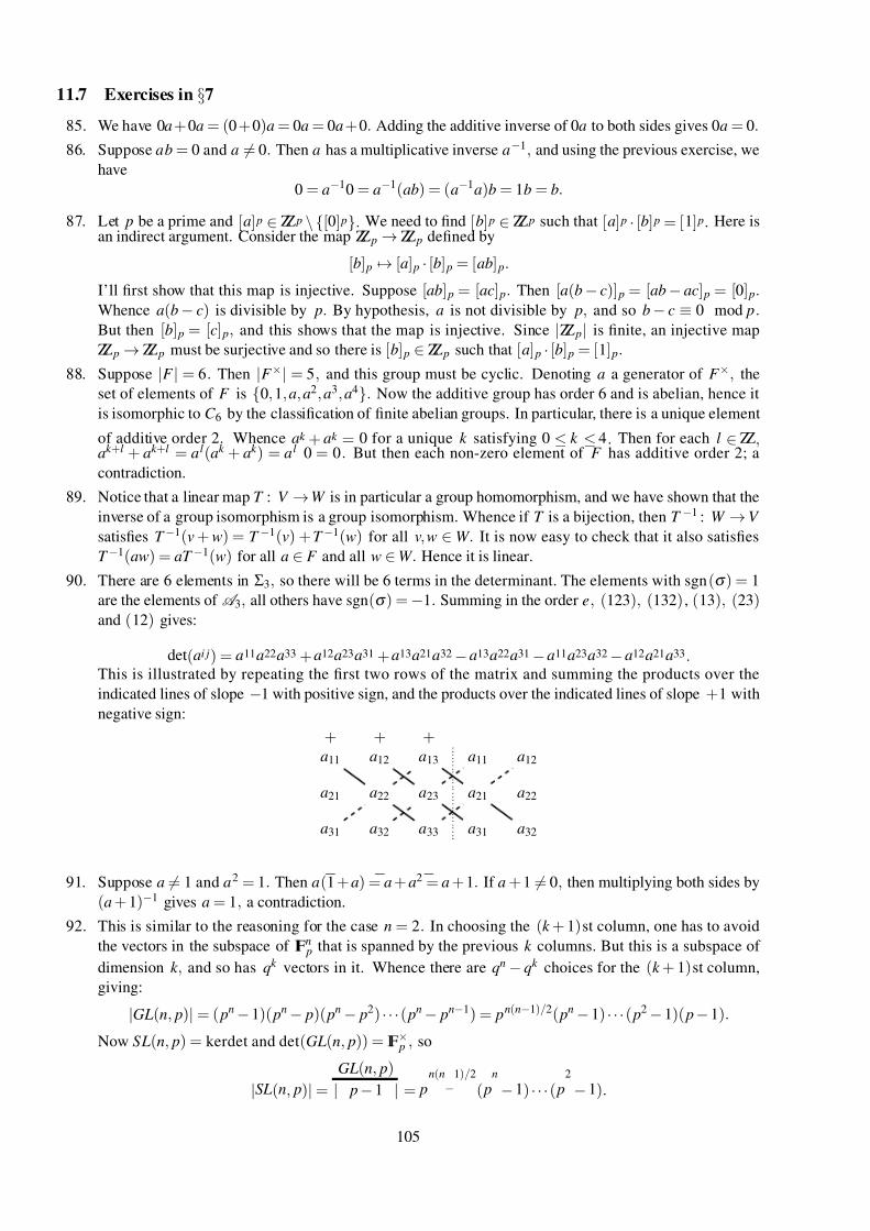
7/26/2019 MATH 2968 Algebra Advanced Notes
http://slidepdf.com/reader/full/math-2968-algebra-advanced-notes 105/110
11.7 Exercises in §7
85. We have 0a + 0a = (0 + 0)a = 0a = 0a + 0. Adding the additive inverse of 0a to both sides gives 0a = 0.
86. Suppose ab = 0 and a = 0. Then a has a multiplicative inverse a−1, and using the previous exercise, we
have
0 = a−10 = a−1(ab) = (a−1a)b = 1b = b.
87. Let p be a prime and [a] p ∈ ZZ p \[0] p. We need to find [b] p ∈ ZZ p such that [a] p · [b] p = [1] p. Here isan indirect argument. Consider the map ZZ p → ZZ p defined by
[b] p → [a] p · [b] p = [ab] p.
I’ll first show that this map is injective. Suppose [ab] p = [ac] p. Then [a(b − c)] p = [ab − ac] p = [0] p.Whence a(b − c) is divisible by p. By hypothesis, a is not divisible by p, and so b − c ≡ 0 mod p.But then [b] p = [c] p, and this shows that the map is injective. Since |ZZ p| is finite, an injective map
ZZ p → ZZ p must be surjective and so there is [b] p ∈ ZZ p such that [a] p · [b] p = [1] p.
88. Suppose |F | = 6. Then |F ×| = 5, and this group must be cyclic. Denoting a a generator of F ×, the
set of elements of F is 0, 1, a, a2, a3, a4. Now the additive group has order 6 and is abelian, hence it
is isomorphic to C 6 by the classification of finite abelian groups. In particular, there is a unique element
of additive order 2. Whence ak + ak = 0 for a unique k satisfying 0 ≤ k ≤ 4. Then for each l ∈ ZZ,ak +l + ak +l = al(ak + ak ) = al 0 = 0. But then each non-zero element of F has additive order 2; a
contradiction.
89. Notice that a linear map T : V → W is in particular a group homomorphism, and we have shown that the
inverse of a group isomorphism is a group isomorphism. Whence if T is a bijection, then T −1 : W → V
satisfies T −1(v + w) = T −1(v) + T −1(w) for all v, w ∈ W . It is now easy to check that it also satisfies
T −1(aw) = aT −1(w) for all a ∈ F and all w ∈ W . Hence it is linear.
90. There are 6 elements in Σ3, so there will be 6 terms in the determinant. The elements with sgn(σ ) = 1
are the elements of A 3, all others have sgn(σ ) = −1. Summing in the order e, (123), (132) , (13), (23)and (12) gives:
det(ai j) = a11a22a33 + a12a23a31 + a13a21a32 − a13a22a31 −a11a23a32 − a12a21a33.This is illustrated by repeating the first two rows of the matrix and summing the products over the
indicated lines of slope −1 with positive sign, and the products over the indicated lines of slope +1 with
negative sign:
a11 a12 a13 a11 a12
a21 a22 a23 a21 a22
a31 a32 a33 a31 a32
+ + +
− − −91. Suppose a = 1 and a2 = 1. Then a(1 + a) = a + a2 = a + 1. If a + 1 = 0, then multiplying both sides by
(a + 1)−1 gives a = 1, a contradiction.
92. This is similar to the reasoning for the case n = 2. In choosing the (k + 1)st column, one has to avoid
the vectors in the subspace of IFn p that is spanned by the previous k columns. But this is a subspace of
dimension k , and so has qk vectors in it. Whence there are qn − qk choices for the (k + 1)st column,
giving:
|GL(n, p)| = ( pn − 1)( pn − p)( pn − p2) · · ·( pn − pn−1) = pn(n−1)/2( pn − 1) · · ·( p2 − 1)( p −1).
Now SL(n, p) = kerdet and det(GL(n, p)) = IF× p , so
|SL(n, p)| = |GL(n, p)
| p − 1 = pn(n
−1)/2
( pn
−1) · · ·( p2
− 1).
105
7/26/2019 MATH 2968 Algebra Advanced Notes
http://slidepdf.com/reader/full/math-2968-algebra-advanced-notes 106/110
93. For the first two parts, you already have examples of elements of orders 2, 3 and 4 in the text. An element
of order 6 is obtained by multiplying an element of order 3 by − E . The isomorphism should be easy to
check.
94. Hint: First establish SL(2, 4) ∼= PSL(2, 4) = PGL(2, 4), and then consider the action of PGL(2, 4) on the
set of all lines in IF24.
95. We already know that the quaternion subgroup is normal, and hence is a union on conjugacy classes.
The analysis can be done in the quaternion group. There are two conjugacy classes with one element
each, the identity and the involution. The 6 elements of order 4 are all conjugate. What remains are the
8 elements of order 3 and the 8 elements of order 6 in SL(2, 3). The elements of order 6 are obtained
from elements of order 3 by multiplying by − E . Since − E is central, A is conjugate to B if and only
if − A is conjugate to − B. So it suffices to determine the conjugacy classes of the elements of order 3.
Since the elements of order 3 fall into the 4 Sylow 3–subgroups, the second Sylow theorem implies that
there is either one conjugacy class of all 8 elements of order 3, or two conjugacy classes of 4 elements
each. I claim that not all 8 elements of order 3 are conjugate. If this were the case, then each element of
order 3 would be conjugate to its inverse. I’ll write ABA−1 = B−1 in the form AB = B−1 A. Consider the
following element of order 3:
B = 1 1
0 1 ,
and try to determine A ∈ SL(2, 3) such that AB = B−1 A:a b
c d
1 1
0 1
=
1 −1
0 1
a b
c d
.
This gives: a a + b
c c + d
=
a − c b −d
c d
The first row gives c = 0 and a = −d . But c = 0 implies that 1 = det A = ad , and so 1 = −a2. Whence
a2 =−
1. But the multiplicative group of IF3 is cyclic of order 2, and so a2 = 1
=
−1 for each invertible
element; a contradiction. Hence B is not conjugate to B−1, and we have 2 conjugacy classes of elements
of order 3 (each containing 4 elements).
96. This is a group of order 8, and it is easy to check that it is non-abelian. Whence it is isomorphic to either
D4 or Q8 by a previous exercise. Now Q8 has a unique involution, and it is not difficult to find at least
two distinct involutions in the group U for p = 2. Alternatively, you can determine elements of order 4
and 2 in U and define a suitable isomorphism U → D4.
97. This is a straight forward computation; for instance using matrices representing the transformations.
106
7/26/2019 MATH 2968 Algebra Advanced Notes
http://slidepdf.com/reader/full/math-2968-algebra-advanced-notes 107/110
11.8 Exercises in §8
98. Having one vertex at e1 = (1, 0) and the y–axis as an axis of symmetry implies that −e1 = (−1, 0) is
also a vertex of the hexagon, and hence the origin (0, 0) is the centre of gravity of the set of vertices.
Whence the set of vertices is the orbit of e1 under the group generated by a rotation by 2π /6 about the
origin.
99. The set of vertices in anti-clockwise order is v1, v2, v2 − v1,−v1,−v2, v1 − v2. It is now a pleasantexercise to work out the matrices representing the group elements. For instance, the anti-clockwise
rotation by 2π /6 about the origin is represented by:0 −1
1 1
.
100. Here are some hints: Use AB = BC . An equation of this form holds for B = 0, so does not imply that B
is invertible. It is easy to see that B has rank 3; applying the row operations that reduce B to E to the
identity matrix E yields the inverse B−1. Conjugation by B corresponds to a change of basis; the desired
basis vectors are the columns in which of the two matrices: B or B−1 ?
101. This holds unless λ = 0.
102. Choose a basis for W , say (w1, . . . , wk ), and extend it to a basis of V , say (w1, . . . , wk , vk +1, . . . , vn). Now
verify that vk +1, . . . , vn ≤ V is a complement of W in V .
103. Suppose B U = (u1, . . . , uk ) and B W = (w1, . . . , wm). Since ϕ (U ) ≤ U , given any u ∈ U , we have
ϕ (u) =∑a ju j =∑a ju j +∑0w j
for some a j ∈ F . An analogous statement holds for vectors in W . Since this is in particular holds for the
basis vectors, we obtain the matrix as claimed.
104. I will not provide a solution at this stage.
105. I will not provide a solution at this stage.
106. I will not provide a solution at this stage.
107. The first part follows from the fact that HomF (V ,V ) is an F –vector space. The second part follows from
the fact that (aϕ k )(bϕ n) = abϕ k +n = (bϕ n)(aϕ k ) for all a, b ∈ F and all n, k ∈ IN.
108. The minimal polynomial mϕ has zero constant term if and only if (mϕ ( x) = x p( x) for some p ∈ F [ x]) if
and only if (0 is an eigenvalue of ϕ ) if and only if (kerϕ is non-trivial) if and only if (ϕ is not invertible).
109. Hint: Write p( x) = xq( x)+a, where q ∈ F [ x] and a ∈ F ×. You know p(ϕ ) = 0. What is a good candidate
for ϕ −1 ?
110. We have mϕ (ϕ ) = 0. Since V = ⊕W k , for any v ∈ V there are wk ∈ W k such that v = ∑wk . Suppose
( p j(ϕ ))s j−1 = 0 ∈ HomF (W j,W j) for some j, and let q = mϕ
p j. Then q ∈ F [ x], q is monic, q divides mϕ
and deg(q) = deg(mϕ )− deg( p j) < deg(mϕ ). Now
q(ϕ )(v) = q(ϕ )(∑wk ) =∑q(ϕ )(wk ) =∑0 = 0,
since for each k = j, q(ϕ ) contains the factor ( pk (ϕ ))sk and ( pk (ϕ ))sk wk = 0 by definition of W k , and
for k = j, we use the hypothesis ( p j(ϕ ))s j−1 = 0 ∈ HomF (W j,W j). Since v was arbitrary, this shows
that q(ϕ ) = 0 ∈ HomF (V ,V ), and so mϕ divides q. But this contradicts deg(q) < deg(mϕ ).
111. If p is a polynomial of degree n, then taking the derivative n + 1 times gives the zero polynomial.
Whence ψ n = 0. Since taking the n th derivative of xn gives n! = 0, the nilpotency degree of ψ is n + 1.
112. For the first part, notice that if λ = 0 is an eigenvalue of ψ , then there is v = 0 such that ψ (v) = λ v.But then for every k ∈ IN, we have ψ k (v) = λ k v = 0, and so ψ k = 0 ∈ HomF (V ,V ). This shows that the
only possible eigenvalue is 0. Since ψ s = 0 for some s ∈ IN, we have kerψ s = V . If kerψ = 0, then
ψ is invertible, and so is every power of ψ . Whence kerψ
=
0
, and 0 is an eigenvalue of ψ .
113. This follows from the fact that ρ is invertible if and only if kerρ = 0.
107
7/26/2019 MATH 2968 Algebra Advanced Notes
http://slidepdf.com/reader/full/math-2968-algebra-advanced-notes 108/110
114. This should be a straight forward enumeration.
115. A direct computation shows A2 = 0. So the maximal length of a forwards orbit is 2. Next compute
the rank of A; the answer should be 3. Whence the nullity of A is 6 − 3 = 3, and hence there will be
exactly 3 Jordan blocks. Since A is a 6 × 6 matrix, the Jordan normal form consists of 3 blocks of size
2. This information completely determines the matrix. To find the corresponding basis, pick 3 linearly
independent vectors with Av
= 0. For instance, e1, e2, e3 have this property and hence assemble the basis;
in this case B = ( Ae1, e1, Ae2, e2, Ae3, e3).
116. There are 5 possibilities for the characteristic polynomial. They split into 14 possibilities for the minimal
polynomial. Except for one case, the minimal polynomial uniquely determined the Jordan normal form;
in the exceptional case one also needs to know the dimension of an eigenspace.
117. The characteristic polynomial is cϕ ( x) = x( x−1)2. So IR3 = ker(ϕ )⊕ker(ϕ −e)2. We compute rk A = 2,so dimker(ϕ ) = 3 − 2 = 1, and hence dimker(ϕ − e)2 = 2. Thus, there is a 1 × 1 block corresponding
to the eigenvalue 0 and either one 2 × 2 block corresponding to the eigenvalue 1 or two 1 × 1 blocks
corresponding to 1. Now compute rk ( A− E ) = 2, so dimker(ϕ −e) = 3−2 = 1 < 2, and hence there is
one 2×2 block corresponding to 1. Now kerϕ =
0
1
−2
and ker(ϕ −e)2 =
1
2
0
,
3
0
10
. Neither
of the latter two vectors is in ker(ϕ − e), so letting b1 =
0
1
−2
, b2 = ( A − E )
1
2
0
and b3 =
1
2
0
gives the desired basis.
118. The decomposition ϕ = δ +η follows from Theorem 8.40. Since conjugation preserves commutativity,
we may assume that ϕ is a direct sum of transformation of the form (dilation + left-shift). Using the
properties of the direct sum, it suffices to consider the situation where ϕ is a transformation of the form
(dilation + left-shift). Denote δ the dilation and η the left-shift. Since δ = λ e for some λ ∈ F , we
have δ ϕ = ϕδ and δ η = ηδ . Whence ηϕ = η(δ +η) = ηδ +η2 = δη +η2 = (δ +η)η = ϕη.
108
7/26/2019 MATH 2968 Algebra Advanced Notes
http://slidepdf.com/reader/full/math-2968-algebra-advanced-notes 109/110
Bibliography
If you need a text to supplement the lectures and notes, there are many books on elementary group theory to
choose from in the library. These books and wikipedia will tell you more than may be good for your progress
in this course, since you may find the answers to questions I’d like you to spend some time to try to solve.
Under textbooks, I list texts that cover large portions of this course at about the same level. The book listedunder bed-time reading has an excellent discussion of symmetry and tilings of the plane, and contains many
beautiful pictures. These books will be on reserve in the library.
The geometry games are related to the study of symmetry in general, and wallpaper groups in particular. Some
of the books listed under further study assume some background knowledge in topology or metric spaces. I
have marked those that are more advanced in style (if not in content) with an asterisk. The references are just
that: papers or books that have been cited in these notes, or been used for their preparation.
Textbooks
[1] Niels Lauritzen: Concrete Abstract Algebra, Cambridge University Press, 2003.
[2] Joseph J. Rotman: An Introduction to the Theory of Groups, Springer Verlag, New York, 1995.
Bed-time reading
[3] David Mumford, Caroline Series and David Wright: Indra’s pearls. The vision of Felix Klein. Cambridge Univer-
sity Press, New York, 2002.
Geometry games and software
[4] Jeffrey Weeks: Topology and Geometry Software, freely available at www.geometrygames.org
Further study
[5] Gilbert Baumslag: Topics in combinatorial group theory. Lectures in Mathematics ETH Zurich. Birkhauser Ver-
lag, Basel, 1993.
[6] Alan F. Beardon: The geometry of discrete groups. Springer-Verlag, New York, 1995.
[7] * Charles Curtis and Irving Reiner: Representation Theory of Finite Groups and Associative Algebras. Reprint of
the 1962 second edition. AMS, 1962.
[8] * Pierre de la Harpe: Topics in Geometric Group Theory, Chicago Lectures in Mathematics. University of Chicago
Press, Chicago, 2000.
[9] * Gordon James and Martin Liebeck: Representations and Characters of Groups, Cambridge University Press,
2001.
[10] Svetlana Katok: Fuchsian groups. Chicago Lectures in Mathematics. University of Chicago Press, Chicago, 1992.
[11] Wilhelm Magnus, Abraham Karrass and Donald Solitar: Combinatorial group theory. Presentations of groups in
terms of generators and relations. Reprint of the 1976 second edition. Dover Publications, Mineola, NY, 2004.
[12] John Meier: Groups, Graphs and Trees: An Introduction to the Geometry of Infinite Groups, London Mathemati-
cal Society Student Texts. Cambridge University Press, 2008.
[13] * Jean-Pierre Serre: Linear Representations of Finite Groups, Springer Verlag, New York, 1977.
[14] John Stillwell: Naive Lie Theory, Springer Verlag, New York, 2010.
[15] * Steven Weintraub: Representation Theory of Finite Groups: Algebra and Arithmetic, AMS, 2003.
109
7/26/2019 MATH 2968 Algebra Advanced Notes
http://slidepdf.com/reader/full/math-2968-algebra-advanced-notes 110/110
References
[16] Roger C. Alperin: An elementary account of Selberg’s lemma, L’Enseignement Mathematique 33 (1987) 269–273.
[17] Marc Lackenby: Topology and Groups. Lecture notes. Available from: http://people.maths.ox.ac.uk/lackenby/
[18] Tristan Needham: Visual Complex Analysis. The Clarendon Press, Oxford University Press, New York, 1997.
[19] William R. Scott: Group Theory. Reprint of the 1964 second edition. Dover Publications, Mineola, NY, 2010.
[20] John R. Stallings: Topology of finite graphs. Invent. Math. 71 (1983), no. 3, 551565.