Math 224 Fall 2017Homework 3 Drew Armstrong

Problems from 9th edition of Probability and Statistical Inference by Hogg, Tanis and Zim-merman:

• Section 2.1, Exercises 6, 7, 8, 12.• Section 2.3, Exercises 1, 3, 4, 12, 13, 14.• Section 2.4, Exercises 12.

Solutions to Book Problems.

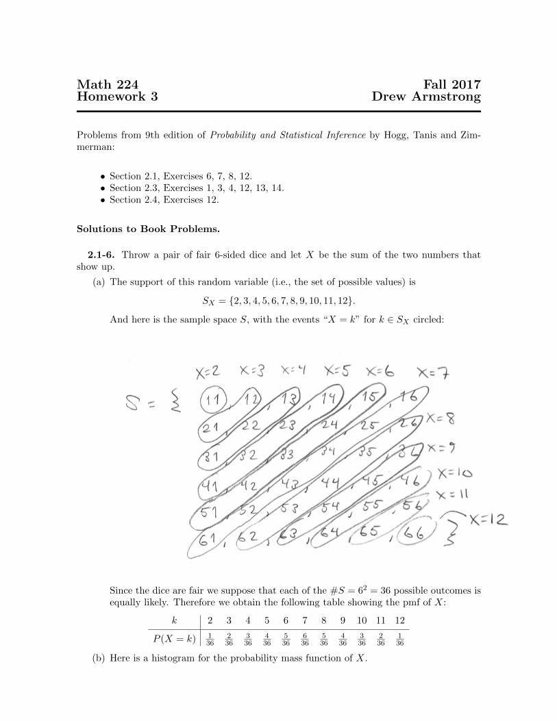
2.1-6. Throw a pair of fair 6-sided dice and let X be the sum of the two numbers thatshow up.

(a) The support of this random variable (i.e., the set of possible values) is

SX = {2, 3, 4, 5, 6, 7, 8, 9, 10, 11, 12}.

And here is the sample space S, with the events “X = k” for k ∈ SX circled:

Since the dice are fair we suppose that each of the #S = 62 = 36 possible outcomes isequally likely. Therefore we obtain the following table showing the pmf of X:

k 2 3 4 5 6 7 8 9 10 11 12

P (X = k) 136

236

336

436

536

636

536

436

336

236

136

(b) Here is a histogram for the probability mass function of X.

2.1-7. Roll two fair 6-sided dice and let X be the minimum of the two numbers that showup. Let Y be the range of the two outcomes, i.e., the absolute value of the difference of thetwo numbers that show up.

(a) The support of X is SX = {1, 2, 3, 4, 5, 6}. Here is the sample space with the events“X = k” circled for each k ∈ SX :

Since the #S = 36 outcomes are equally likely we obtain the following table showingthe pmf of X:

k 1 2 3 4 5 6

P (X = k) 1136

936

736

536

336

136

(b) And here is a histogram for the pmf of X:

(c) The support of Y is SY = {0, 1, 2, 3, 4, 5}. Here is the sample space with the events“Y = k” circled for each k ∈ SY :

Since the #S = 36 outcomes are equally likely we obtain the following table showingthe pmf of Y :

k 0 1 2 3 4 5

P (Y = k) 636

1036

836

636

436

236

(d) And here is a histogram for the pmf of Y .

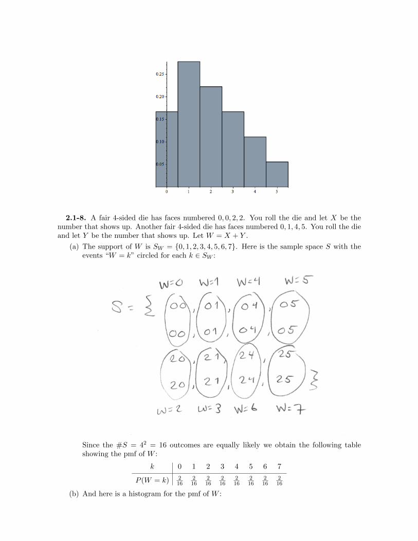
2.1-8. A fair 4-sided die has faces numbered 0, 0, 2, 2. You roll the die and let X be thenumber that shows up. Another fair 4-sided die has faces numbered 0, 1, 4, 5. You roll the dieand let Y be the number that shows up. Let W = X + Y .

(a) The support of W is SW = {0, 1, 2, 3, 4, 5, 6, 7}. Here is the sample space S with theevents “W = k” circled for each k ∈ SW :

Since the #S = 42 = 16 outcomes are equally likely we obtain the following tableshowing the pmf of W :

k 0 1 2 3 4 5 6 7

P (W = k) 216

216

216

216

216

216

216

216

(b) And here is a histogram for the pmf of W :

2.1-12. Let X be the number of accidents per week in a factory and suppose that the pmfof X is given by

fX(k) = P (X = k) =1

(k + 1)(k + 2)=

1

k + 1− 1

k + 2for k = 0, 1, 2, . . .

Find the conditional probability of X ≥ 4, given that X ≥ 1.

Solution: Let A = “X ≥ 4” and B = “X ≥ 1” and note that A ⊆ B, which implies thatA ∩B = A. Now we are looking for the conditional probability

P (A|B) =P (A ∩B)

P (B)=P (A)

P (B)=P (X ≥ 4)

P (X ≥ 1).

To compute P (X ≥ 4) and P (X ≥ 1), let us first investigate why P (S) = P (X ≥ 0) = 1.This is because we have a “telescoping” infinite series:

P (X ≥ 0) = P (X = 0) + P (X = 1) + P (X = 2) + · · ·

=

(1−

���1

2

)+

(���1

2−

���1

3

)+

(���1

3−

���1

4

)+ · · ·

= 1 + 0 + 0 + 0 + · · ·= 1.

The same idea shows us that P (X ≥ n) = 1/(n+ 1) for any n. Indeed, we have

P (X ≥ n) = P (X = n) + P (X = n+ 1) + P (X = n+ 2) + · · ·

=

(1

n+ 1−���1

n+ 2

)+

(�

��1

n+ 2−�

��1

n+ 3

)+

(�

��1

n+ 3−�

��1

n+ 4

)+ · · ·

=1

n+ 1+ 0 + 0 + 0 + · · ·

=1

n+ 1.

Finally, we conclude that

P (X ≥ 4 |X ≥ 1) =P (X ≥ 4)

P (X ≥ 1)=

1/5

1/2=

2

5.

///

2.3-1. Find the mean and variance of the following distributions:

(a) f(k) = 1/5 for k = 5, 10, 15, 20, 25. Solution: The mean is

µ =∑k

k · f(k) = 5 · 1

5+ 10 · 1

5+ 15 · 1

5+ 20 · 1

5+ 25 · 1

5=

75

5= 15.

To compute the variance we will use the following table:

k 5 10 15 20 25

µ 15 15 15 15 15

(k − µ)2 100 25 0 25 100

f(k) 1/5 1/5 1/5 1/5 1/5

Then we have

σ2 =∑k

(k − µ)2 · f(k) = 100 · 1

5+ 25 · 1

5+ 0 · 1

5+ 25 · 1

5+ 100 · 1

5=

250

5= 50.

(b) f(x) = 1 for k = 5. Solution: The mean is

µ =∑k

k · f(k) = 5 · 1 = 5

and the variance is

σ2 =∑k

(k − µ)2 · f(k) = (5− 5)2 · 1 = 0.

(c) f(k) = (4− k)/6 for k = 1, 2, 3. Solution: The mean is

µ =∑k

k · f(k) = 1 · 4− 1

6+ 2 · 4− 2

6+ 3 · 4− 3

6=

13

6=

10

6=

5

3.

To compute the variance we use the following table:

k 1 2 3

µ 5/3 5/3 5/3

(k − µ)2 4/9 1/9 16/9

f(k) 3/6 2/6 1/6

Then we have

σ2 =∑k

(k − µ)2 · f(k) =4

9· 3

6+

1

9· 2

6+

16

9· 1

6=

30

54=

5

9.

2.3-3. Given E(X = 4) = 10 and E[(X + 4)2] = 116, determine

(a) Var(X + 4) Solution: Let Y = X + 4. Then

Var(Y ) = E[Y 2]− E[Y ]2

Var(X + 4) = E[(X + 4)2]− E[X + 4]2

= 116− 102

= 16.

(b) µ = E[X] Solution: Since 4 is constant (i.e., it is not random) we have E[4] = 4 andthen by linearity of expectation we have

E[X + 4] = 10

E[X] + E[4] = 10

E[X] + 4 = 10

E[X] = 6.

(c) σ2 = Var(X) Solution: We want to compute

Var(X) = E[X2]− E[X]2

and we already know that E[X] = 6, so it only remains to compute E[X2]. To do this,we use linearity:

E[(X + 4)2] = 116

E[X2 + 8X + 16] = 116

E[X2] + 8E[X] + 16 = 116

E[X2] + 8 · 6 = 100

E[X2] + 48 = 100

E[X2] = 52.

We conclude that

σ2 = Var(X) = E[X2]− E[X]2 = 52− 62 = 56− 36 = 16,

and hence also σ =√

16 = 4.

2.3-4. Let µ and σ2 be the mean and variance of the random variable X. Determine

E[(X − µ)/σ] and E[((X − µ)/σ)2

]Solution: Since µ and σ are constant (i.e., not random) we use linearity to get

E

[X − µσ

]= E

[1

σX − µ

σ

]=

1

σE[X]− E

[µσ

]=

1

σ· µ− µ

σ= 0.

Similarly, we have

E

[(X − µσ

)2]

= E

[1

σ2(X − µ)2

]=

1

σ2E[(X − µ)2

]=

1

σ2· σ2 = 1.

We conclude that the random variable (X − µ)/σ has mean 0 and variance 1 (hence alsostandard deviation 1). I wonder if that’s useful for something. ///

2.3-12. Let X be the number of people selected at random that you must ask in order tofind someone with the same birthday as yours. (Assume that each day of the year is equallylikely and ignore February 29.)

(a) What is the pmf of X? Answer: Assuming that people’s birthdays are independent,we can treat each person as a coin flip with

H = “same birthday as yours,”

T = “different birthday.”

Since all birthdays are equally likely we have P (H) = 1/365. Then the occurrence ofthe “first head” is a geometric random variable with pmf

P (X = k) = P (T )k−1P (H) =

(364

365

)k−1( 1

365

)=

364k−1

365k.

(b) Give the values of the mean, variance, and standard deviation of X. Answer: If X isa geometric random variable with probability of heads P (H) = p then the table in thefront of the book tells us that

µ =1

pand σ2 =

1− pp2

.

In our case we have

µ =1

1/365= 365 and σ2 =

364/365

(1/365)2= 364 · 365 = 132860,

hence also σ =√

132860 ≈ 364.5.

(c) Find P (X > 400) and P (X < 300). Answer: In general, for a geometric randomvariable X and an integer n we have

P (X > n) =∑k>n

P (X = k)

=∞∑

k=n+1

(1− p)k−1p

= (1− p)np+ (1− p)n+1p+ (1− p)n+2p+ · · ·= (1− p)np

(1 + (1− p) + (1− p)2 + (1− p)3 + · · ·

)= (1− p)np · 1

1− (1− p)

= (1− p)np · 1

p

= (1− p)n.

Therefore in our case we have

P (X > 400) = (1− p)400 =

(364

365

)400

≈ 33.37%

and

P (X < 300) = 1− P (X ≥ 300) = 1− P (X > 299) = 1−(

364

365

)299

≈ 55.97%.

Remark: Here is a picture illustrating the results of the previous problem:

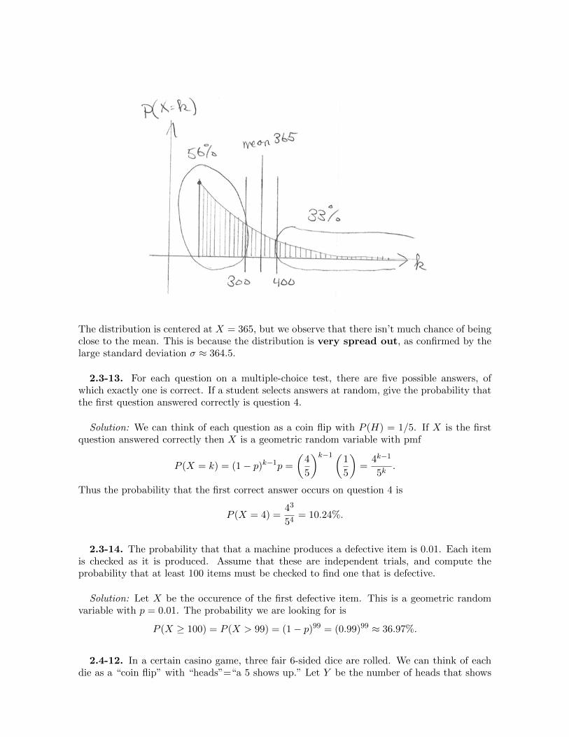
The distribution is centered at X = 365, but we observe that there isn’t much chance of beingclose to the mean. This is because the distribution is very spread out, as confirmed by thelarge standard deviation σ ≈ 364.5.

2.3-13. For each question on a multiple-choice test, there are five possible answers, ofwhich exactly one is correct. If a student selects answers at random, give the probability thatthe first question answered correctly is question 4.

Solution: We can think of each question as a coin flip with P (H) = 1/5. If X is the firstquestion answered correctly then X is a geometric random variable with pmf

P (X = k) = (1− p)k−1p =

(4

5

)k−1(1

5

)=

4k−1

5k.

Thus the probability that the first correct answer occurs on question 4 is

P (X = 4) =43

54= 10.24%.

2.3-14. The probability that that a machine produces a defective item is 0.01. Each itemis checked as it is produced. Assume that these are independent trials, and compute theprobability that at least 100 items must be checked to find one that is defective.

Solution: Let X be the occurence of the first defective item. This is a geometric randomvariable with p = 0.01. The probability we are looking for is

P (X ≥ 100) = P (X > 99) = (1− p)99 = (0.99)99 ≈ 36.97%.

2.4-12. In a certain casino game, three fair 6-sided dice are rolled. We can think of eachdie as a “coin flip” with “heads”=“a 5 shows up.” Let Y be the number of heads that shows

up, which has a binomial pmf:

P (Y = k) =

(3

k

)(1

6

)k (5

6

)3−k.

The support of Y is SY = {0, 1, 2, 3} and your winnings in the game are determined by anotherrandom variable X, which is defined by

X =

−$1 if Y = 0

$1 if Y = 1

$2 if Y = 2

$3 if Y = 3

(a) The support of X is SX = {−1, 1, 2, 3} and the following table shows the pmf of X:

k −1 1 2 3

P (X = k) 53

633 · 52

633 · 5

63163

(b) Therefore the mean of X (i.e., your expected winnings) is

µ = E[X] =∑k∈SX

kP (X = k)

= −1 · 53

63+ 1 · 3 · 52

63+ 2 · 3 · 5

63+ 3 · 1

63

=−53 + 3 · 52 + 6 · 5 + 3

63=−17

216≈ −$0.0787.

That is, you should expect to lose about 8 cents on this game. To compute the variancewe use the following table:

k −1 1 2 3

(k − µ)2 3960146656

5428946656

20160146656

44222546656

P (X = k) 53

633 · 52

633 · 5

63163

We find that

σ2 = Var(X) =∑k∈SX

(k − µ)2P (X = k) =57815

46656≈ 1.239,

and hence the standard deviation is

σ =√

57815/46656 ≈ 1.113.

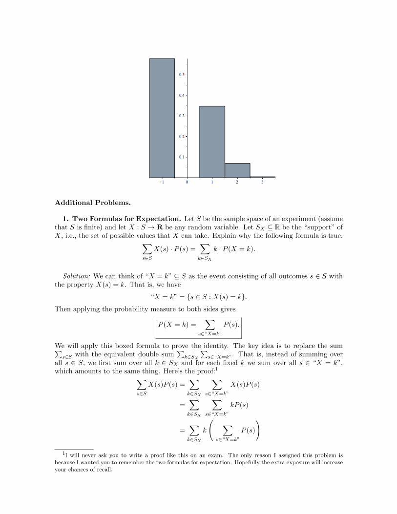
(c) And here is a histogram for the pmf of your winnings:

Additional Problems.

1. Two Formulas for Expectation. Let S be the sample space of an experiment (assumethat S is finite) and let X : S → R be any random variable. Let SX ⊆ R be the “support” ofX, i.e., the set of possible values that X can take. Explain why the following formula is true:∑

s∈SX(s) · P (s) =

∑k∈SX

k · P (X = k).

Solution: We can think of “X = k” ⊆ S as the event consisting of all outcomes s ∈ S withthe property X(s) = k. That is, we have

“X = k” = {s ∈ S : X(s) = k}.

Then applying the probability measure to both sides gives

P (X = k) =∑

s∈“X=k”

P (s).

We will apply this boxed formula to prove the identity. The key idea is to replace the sum∑s∈S with the equivalent double sum

∑k∈SX

∑s∈“X=k”. That is, instead of summing over

all s ∈ S, we first sum over all k ∈ SX and for each fixed k we sum over all s ∈ “X = k”,which amounts to the same thing. Here’s the proof:1∑

s∈SX(s)P (s) =

∑k∈SX

∑s∈“X=k”

X(s)P (s)

=∑k∈SX

∑s∈“X=k”

kP (s)

=∑k∈SX

k

( ∑s∈“X=k”

P (s)

)

1I will never ask you to write a proof like this on an exam. The only reason I assigned this problem isbecause I wanted you to remember the two formulas for expectation. Hopefully the extra exposure will increaseyour chances of recall.

=∑k∈SX

kP (X = k).

///

2. Expected Value of a Binomial Random Variable.

(a) Use the explicit formula for binomial coefficients to prove that

k

(n

k

)= n

(n− 1

k − 1

).

Solution 1: The right hand side is given by

n

(n− 1

k − 1

)=

n(n− 1)!

(k − 1)! [(n− 1)− (k − 1)]!=

n!

(k − 1)!(n− k)!

and the left hand side is given by

k

(n

k

)=

k

k!· n!

(n− k)!=

1

(k − 1)!· n!

(n− k)!=

n!

(k − 1)!(n− k)!.

Note that the formulas are the same. ///

Solution 2: A club of k people is selected from a classroom of n students. Onemember of the club is chosen to be the president. In how many ways can we choosethe club? One the one hand, there are

(nk

)ways to choose the club members and then

k ways to choose the president from the club members, for a total of

k

(n

k

)choices.

On the other hand, we could choose one student from the class to be the president ofthe club. There are n ways to do this. Then, we choose k − 1 of the remaining n− 1students to be the other members of the club. There are

(n−1k−1)

ways to do this, for atotal of

n

(n− 1

k − 1

)choices.

Since these two formulas count the same thing, they must be equal. ///

(b) Use part (a) to compute the expected value of a binomial random variable:

E[X] =n∑

k=0

k

(n

k

)pk(1− p)n−k

=n∑

k=1

k

(n

k

)pk(1− p)n−k

=

n∑k=1

n

(n− 1

k − 1

)pk(1− p)n−k

= n

n∑k=1

(n− 1

k − 1

)pk(1− p)n−k

= n

n−1∑`=0

(n− 1

`

)p`+1(1− p)n−(`+1)

= np ·n−1∑`=0

(n− 1

`

)p`(1− p)(n−1)−`

= np · (p+ (1− p))n−1

= np · 1n−1

= np.

///

Remark: In class we saw an alternate way to compute the expected value of a binomialrandom variable. Flip a coin n times and let Xi be the “number of heads” that occur on theith coin flip. That is, let

Xi =

{1 if the ith flip is H,

0 if the ith flip is T .

Each Xi has a so-called Bernoulli distribution, with pmf given by the following table:

k 0 1

P (Xi = k) 1− p p

And hence each Xi has expected value

E[Xi] = 0 · P (Xi = 0) + 1 · P (Xi = 1) = 0 · (1− p) + 1 · p = p.

By adding the random variables X1, X2, . . . , Xn we obtain a binomial random variable:

(total # heads) = (# heads on 1st flip) + · · ·+ (# heads on nth flip)

X = X1 +X2 + · · ·+Xn.

And then the linearity of expectation gives

E[X] = E[X1 +X2 + · · ·+Xn]

= E[X1] + E[X2] + · · ·+ E[Xn]

= p+ p+ · · ·+ p

= np.

Which method do you like better?