Mach Learn (2013) 90:127–160DOI 10.1007/s10994-012-5303-x

Mass estimation

Kai Ming Ting · Guang-Tong Zhou · Fei Tony Liu ·Swee Chuan Tan

Received: 17 June 2011 / Revised: 20 May 2012 / Accepted: 1 June 2012 / Published online: 26 June 2012© The Author(s) 2012

Abstract This paper introduces mass estimation—a base modelling mechanism that canbe employed to solve various tasks in machine learning. We present the theoretical basis ofmass and efficient methods to estimate mass. We show that mass estimation solves problemseffectively in tasks such as information retrieval, regression and anomaly detection. Themodels, which use mass in these three tasks, perform at least as well as and often better thaneight state-of-the-art methods in terms of task-specific performance measures. In addition,mass estimation has constant time and space complexities.

Keywords Mass estimation · Density estimation · Information retrieval · Regression ·Anomaly detection

1 Introduction

‘Estimation of densities is a universal problem of statistics (knowing the densities onecan solve various problems).’ —Vapnik (2000).

Density estimation has been the base modelling mechanism used in many techniquesdesigned for tasks such as classification, clustering, anomaly detection and information

Editor: Tong Zhang.

K.M. Ting (�) · F.T. Liu · S.C. TanGippsland School of Information Technology, Monash University, Melbourne, Vic 3842, Australiae-mail: kaiming.ting@monash.edu

F.T. Liue-mail: tony.liu@monash.edu

S.C. Tane-mail: james.tan@monash.edu

G.-T. ZhouSchool of Computing Science, Simon Fraser University, Burnaby, BC, V5A 1S6, Canadae-mail: zhouguangtong@gmail.com

128 Mach Learn (2013) 90:127–160

retrieval. For example in classification, density estimation is employed to estimate theclass-conditional density function (or likelihood function) p(x|j) or posterior probabilityp(j |x)—the principal function underlying many classification methods; e.g., mixture mod-els, Bayesian networks, Naive Bayes. Examples of density estimation include kernel densityestimation, k-nearest neighbours density estimation, maximum likelihood procedures andBayesian methods.

Ranking data points in a given data set in order to differentiate core points from fringepoints in a data cloud is fundamental in many tasks, including anomaly detection and in-formation retrieval. Anomaly detection aims to rank anomalous points higher than normalpoints; information retrieval aims to rank points similar to a query higher than dissimi-lar points. Many existing methods (e.g., Bay and Schwabacher 2003; Breunig et al. 2000;Zhang and Zhang 2006) have employed density to provide the ranking; but density estima-tion is not designed to provide a ranking.

We show in this paper that a new base modelling mechanism called mass estimationpossesses different properties from those offered by density estimation:

• A mass distribution stipulates an ordering from core points to fringe points in a datacloud. In addition, this ordering accentuates the fringe points with a concave functionderived from data, resulting in fringe points having markedly smaller mass than pointsclose to the core points.

• Mass estimation is more efficient than density estimation because mass is computed bysimple counting and it requires only a small sample through an ensemble approach. Den-sity estimation (often used to estimate p(x|j) and p(j |x)) requires a large sample sizein order to have a good estimation and is computationally expensive in terms of time andspace complexities (Duda et al. 2001).

Mass estimation has two advantages in relation to efficacy and efficiency. First, the con-cavity property mentioned above ensures that fringe points are ‘stretched’ to be farther fromthe core points in a mass space—making it easier to separate fringe points from those pointsclose to core points. This property in mass space can then be exploited by a machine learningalgorithm to achieve a better result for the intended task than applying the same algorithmin the original space without this property. We show the efficacy of mass in improving thetask-specific performance of four existing state-of-the-art algorithms in information retrievaland regression tasks. The significant improvements are achieved through a simple mappingfrom the original space to a mass space using the mass estimation mechanism introduced inthis paper.

Second, mass estimation offers to solve a ranking problem more efficiently using theordering derived from data directly—without expensive distance (or related) calculations.An example of inefficient application is in anomaly detection tasks where many methodshave employed distance or density to provide the required ranking. An existing state-of-the-art density-based anomaly detector LOF (Breunig et al. 2000) (which has quadratic timecomplexity) completes a job involving half a million data points in more than five hours;yet the mass-based anomaly detector we have introduced here completes it in less than 20seconds! Section 6.3 provides the details of this example.

The rest of the paper is organised as follows. Section 2 introduces mass and mass es-timation, together with their theoretical properties. We also describe methods for one-dimensional mass estimation. We extend one-dimensional mass estimation to multi-dimensional mass estimation in Sect. 3. We provide an implementation of multi-dimensionalmass estimation in Sect. 4. Section 5 describes a mass-based formalism which serves as abasis of applying mass to different data mining tasks. We realise the formalism in three

Mach Learn (2013) 90:127–160 129

different tasks: information retrieval, regression and anomaly detection, and report the em-pirical evaluation results in Sect. 6. The relations to kernel density estimation, data depth andother related work are described in Sects. 7, 8 and 9, respectively. We provide conclusionsand suggest future work in the last section.

2 Mass and mass estimation

Data mass or mass, in its simplest form, is defined as the number of points in a region. Anytwo groups of data in the same domain have the same mass if they have the same numberof points, regardless of the characteristics of the regions they occupy (e.g., density, shapeor volume). Mass in a given region is thus defined by a rectangular function which has thesame value for the entire region in which the mass is measured.

To estimate the mass for a point and thus the mass distribution of a given data set, a moresophisticated form is required. The intuition is based on the simplest form described above,but multiple (overlapping) regions covering a point are generated. The mass for the pointis then derived from an average of masses from all regions covering the point. We showtwo ways to define these regions. The first is to generate all possible regions through binarysplits from the given data points; and the second is to generate random axis-parallel regionswithin the confine covered by a data sample. The first is described in this section and thesecond is described in Sect. 3.

Each region can be defined in multiple levels where a higher level region covering apoint has a smaller volume than that of a lower level region covering the same point. Weshow that the mass distribution has special properties: (i) the mass distribution defined bylevel-1 regions is a concave function which has the maximum mass at the centre of the datacloud, irrespective of its density distribution, including uniform and U-shape distributions;and (ii) higher level regions are required to model multi-modal mass distributions.

Note that mass is not a probability mass function, and it does not provide a probability,as the probability density function does through integration.

In Sect. 2.1, we show (i) how to estimate a mass distribution for a given data set throughbinary splits and (ii) the theoretical properties of mass estimation. Section 2.2 describes anapproximation to the theoretical mass estimation which works more efficiently in practice.The symbols and notations used are provided in Table 1.

Table 1 Symbols and notations

Ru A real domain of u dimensions

x A one-dimensional instance in Rx An instance in Ru

D A data set of x, where |D| = n

D A subset of D, where |D| = ψ

z An instance in Rt

D′ A data set of z

c The ensemble size used to estimate mass

h Level of mass distribution

t Number of mass distributions in m̃ass(·)mi(·) Mass base function defined using binary split si

mass(·) Mass function which returns a real value in one-dimensional mass space

m̃ass(·) Mass function which returns a vector of t values in t-dimensional mass space

130 Mach Learn (2013) 90:127–160

2.1 Mass distribution estimation

In this section, we first show in Sect. 2.1.1 a mass distribution estimation that uses binarysplits in the one-dimensional setting, where each binary split separates the one-dimensionalspace into two non-empty regions. In Sect. 2.1.2, we then generalise the treatment usingmultiple levels of binary splits.

2.1.1 Mass distribution estimation using binary splits

Here, we employ a binary split to divide the data set into two separate regions and computethe mass in each region. The mass distribution at point x is estimated to be the sum of all‘weighted’ masses from regions occupied by x, as a result of n − 1 binary splits for a dataset of size n.

Let x1 < x2 < · · · < xn−1 < xn on the real line,1 xi ∈ R and n > 1. Let si be the binarysplit between xi and xi+1, yielding two non-empty regions having two masses mL

i and mRi .

Definition 1 Mass base function: mi(x) as a result of si , is defined as

mi(x) ={

mLi if x is on the left of si

mRi if x is on the right of si

Note that mLi = n − mR

i = i.

Definition 2 Mass distribution: mass(xa) for a point xa ∈ {x1, x2, . . . , xn−1, xn} is definedas a summation of a series of mass base functions mi(x) weighted by p(si) over n− 1 splitsas follows, where p(si) is the probability of selecting si .

mass(xa) =n−1∑i=1

mi(xa)p(si)

=n−1∑i=a

mLi p(si) +

a−1∑j=1

mRj p(sj )

=n−1∑i=a

ip(si) +a−1∑j=1

(n − j)p(sj ) (1)

Note that we have defined∑r

i=q f (i) = 0, when r < q for any function f .

Example For an example of five points x1 < x2 < x3 < x4 < x5, Fig. 1 shows the resultantmi(x) due to each of the four binary splits s1, s2, s3, s4; and their associated masses over foursplits are given below:

mass(x1) = 1p(s1) + 2p(s2) + 3p(s3) + 4p(s4)

mass(x2) = 4p(s1) + 2p(s2) + 3p(s3) + 4p(s4)

mass(x3) = 4p(s1) + 3p(s2) + 3p(s3) + 4p(s4)

mass(x4) = 4p(s1) + 3p(s2) + 2p(s3) + 4p(s4)

mass(x5) = 4p(s1) + 3p(s2) + 2p(s3) + 1p(s4)

1In data having a pocket of points of the same value, an arbitrary order can be ‘forced’ by adding increasingmultiples of an insignificant small value ε to each subsequent point of the pocket, without changing thegeneral distribution.

Mach Learn (2013) 90:127–160 131

Fig. 1 Examples of mass base function mi(x) due to each of the four binary splits: s1, s2, s3, s4

For a given data set, p(si) can be estimated on the real line as p(si) = (xi+1 − xi)/

(xn − x1) > 0, as a result of a random selection of splits based on a uniform distribution.2

For a point x /∈ {x1, x2, . . . , xn−1, xn}, mass(x) is defined as an interpolation between twomasses of adjacent points xi and xi+1, where xi < x < xi+1.

Theorem 1 mass(xa) is maximised at a = n/2 for any density distribution of {x1, . . . , xn};and the points xa , where x1 < x2 < · · · < xn−1 < xn on the real line, can be ordered basedon mass as follows.

mass(xa) < mass(xa+1), a < n/2

mass(xa) > mass(xa+1), a > n/2

Proof The difference in mass between two consecutive points xa and xa+1 differs in onlyone term, i.e., the mass associated with p(sa); and ∀i �= a, the terms for p(si) have the samemass.

2The estimated mass(x) values can be calibrated to a finite data range Δ by multiplying a factor (xn −x1)/Δ.

132 Mach Learn (2013) 90:127–160

mass(xa) − mass(xa+1) =n−1∑i=a

ip(si) +a−1∑j=1

(n − j)p(sj )

−n−1∑

i=(a+1)

ip(si) −a∑

j=1

(n − j)p(sj )

= ap(sa) − (n − a)p(sa)

= (2a − n)p(sa) (2)

Thus,

sign(mass(xa) − mass(xa+1)

) =⎧⎨⎩

negative if a < n/20 if a = n/2positive if a > n/2

The point xn/2 can be regarded as the median. Note that the number of points with themaximum mass depends on whether n is odd or even: When n is an odd integer, only onepoint has the maximum mass at xmedian, where median = �n/2�; when n is an even integer,two points have the maximum mass at a = n/2 and a = 1 + n/2. �

Theorem 2 mass(xa) is a concave function defined w.r.t. {x1, x2, . . . , xn}, when p(si) =(xi+1 − xi)/(xn − x1) for n > 2.

Proof We only need to show that the gradient of xa is non-increasing, i.e., g(xa) > g(xa+1)

for each a.Let g(xa) be the gradient between xa and xa+1, and from (2):

g(xa) = mass(xa+1) − mass(xa)

xa+1 − xa

= n − 2a

xn − x1

The result follows: g(xa) > g(xa+1) for a ∈ {1,2, . . . , n − 1}. �

Corollary 1 A mass distribution estimated using binary splits stipulates an ordering, basedon mass, of the points in a data cloud from xn/2 (with the maximum mass) to the fringepoints (with the minimum mass at either side of xn/2), irrespective of the density distributionincluding uniform density distribution.

Corollary 2 The concavity of mass distribution stipulates that fringe points have markedlysmaller mass than points close to xn/2.

The implication from Corollary 2 is that fringe points are ‘stretched’ to be farther awayfrom the median in a mass space than in the original space—making it easier to separatefringe points from those points close to the median. The mass space is mapped from theoriginal space through mass(x). This property in mass space can then be exploited by amachine learning algorithm to achieve a better result for the intended task than applying thesame algorithm in the original space without this property. We will show that this simplemapping significantly improves the performance of four existing algorithms in informationretrieval and regression tasks in Sects. 6.1 and 6.2.

Equation (1) is sufficient to provide a mass distribution corresponding to a unimodaldensity function or a uniform density function. To better estimate multi-modal mass dis-tributions, multiple levels of binary splits need to be carried out. This is provided in thefollowing.

Mach Learn (2013) 90:127–160 133

Fig. 2 Two examples of massLi(x,h = 1) and massR

i(x,h = 1) due to si=7 and si=11 in the process to get

mass(x,h = 2) from a data set of 20 points with uniform density distribution. The resultant mass(x,h = 2)

is shown in Fig. 3(a)

2.1.2 Level-h mass distribution estimation

If we treat the mass estimation defined in the last subsection as level-1 estimation, thenlevel-h estimation can be viewed as localised versions of the basic level-1 estimation.

Definition 3 The level-h mass distribution for a point xa ∈ {x1, . . . , xn}, where h < n, isexpressed as

mass(xa, h) =n−1∑i=1

massi (xa, h-1)p(si)

=n−1∑i=a

massLi (xa, h-1)p(si)

+a−1∑j=1

massRj (xa, h-1)p(sj ) (3)

Here a high level mass distribution is computed recursively by using the mass distribu-tions obtained at lower levels. A binary split si in a level-h(> 1) mass distribution producestwo level-(h-1) mass distributions: (a) massL

i (x,h-1)—the mass distribution on the left ofsplit si which is defined using {x1, . . . , xi}; and (b) massR

i (x,h-1)—the mass distributionon the right which is defined using {xi+1, . . . , xn}. Equation (1) is the mass distribution atlevel-1.

Figure 2 shows two (out of 19 splits) required to compute level-2 mass estimation,mass(x,h = 2), from a data set of 20 points. Each split produces two level-1 mass estima-tions: massL

i (x,h = 1) and massRi (x,h = 1). Note that level-1 mass distribution is concave,

as proven in Theorem 2. This example shows the results of two splits si=7 and si=11, whereeach level-1 mass distribution is concave.

Using the same analysis as in the proof for Theorem 1, the above equation can be re-expressed as:

mass(xa+1, h) = mass(xa, h) +{ [massR

a (xa, h-1) − massLa (xa, h-1)]p(sa), h > 1

(n − 2a)p(sa), h = 1(4)

As a result, only the mass for the first point x1 needs to be computed using (3). Note thatit is more efficient to compute the mass distribution from the above equation which has timecomplexity O(nh+1); the computation using (3) has complexity O(nh+2).

134 Mach Learn (2013) 90:127–160

Fig. 3 Examples of level-h mass distribution for h = 1,2,3 and density distribution from kernel densityestimation: Gaussian kernel with bandwidth = 0.1 (for the first three figures) and 0.01 (for the last figure inorder to show the density spike). The data sets have 20 points each for the first three figures, and the last onehas 50 points

Definition 4 A level-h mass distribution stipulates an ordering of the points in a data cloudfrom α-core points to the fringe points. Let α-neighbourhood of a point x be defined asNα(x) = {y ∈ D|dist(x, y) ≤ α} for some distance function dist(·, ·). Each α-core point x∗in a data cloud has the highest mass value ∀x ∈ Nα(x

∗). A small α defines local core point(s);and a large α, which covers the entire value range for x, defines global core point(s).

Examples of level-h mass estimation in comparison with kernel density estimation areprovided in Fig. 3. Note that h = 1 mass estimation looks at the data as a group, and itproduces a concave function. As a result, an h = 1 mass estimation always has its globalcore point(s) at the median, regardless of the underlying density distribution—see the fourexamples of h = 1 mass estimation in Fig. 3.

For h > 1 mass distribution, though there is no guarantee for a concave function anymore as a whole, our simulation shows that each cluster within the data cloud (if they ex-ist) exhibits a concave function and it becomes more distinct (as a concave function) as h

increases. An example is shown in Fig. 3(b) which has a trimodal density distribution. No-tice that the h > 1 mass distributions have three α-core points for some α, e.g., 0.2. Otherexamples are shown in Figs. 3(c) and 3(d).

Traditionally, one can estimate the core-ness or the fringe-ness of non-uniformly dis-tributed data to some degree by using density or distance (but not in uniform density distribu-tion). Mass allows one to do that in any distribution without density or distance calculation—the key computational expense in all methods that employ them. For example in Fig. 3(c)which has a skew density distribution, the distinction between near fringe points and far

Mach Learn (2013) 90:127–160 135

fringe points are less obvious using density, unless distances are computed to reveal thedifference. In contrast, mass distribution depicts the relative distance from xmedian using thefringe points’ mass values, without further calculation.

Figure 3(d) shows an example where there are clustered anomalies which are denser thanthe normal points (shown in the bigger cluster on the left of the figure). Anomaly detectionbased on density will identify all these clustered anomalies as more ‘normal’ than the normalpoints because anomalies are defined as points having low density. In sharp contrast, h = 1mass estimation will correctly rank them as anomalies which have the third lowest massvalues. These points are interpreted as points at the fringe of the data cloud of normal pointswhich have higher mass values.

This section has described properties of mass distribution from a theoretical perspective.Though it is possible to estimate mass distribution using (1) and (3), they are limited by itshigh computational cost. We suggest a practical mass estimation method in the next subsec-tion. We use the term ‘mass estimation’ and ‘mass distribution estimation’ interchangeablyhereafter.

2.2 Practical one-dimensional level-h mass estimation

Here we devise an approximation to (3) using random subsamples from a given data set.

Definition 5 mass(x,h|D) is the approximate mass distribution for a point x ∈ R, definedw.r.t. D = {x1, . . . , xψ }, where D is a random subset of the given data set D, and ψ |D|,h < ψ .

Here we employ a rectangular function to define mass for a region encompassing eachpoint x ∈ D. mass(x,h|D) is implemented using a lookup table where a region for each pointxi ∈ D covers a range (xi−1 + xi)/2 ≤ x < (xi+1 + xi)/2 and has the same mass(xi, h|D)

value for the entire region. The range for each of the two end-points is set to have equallength on either side of the point. An example is provided in Fig. 4(a).

In addition, a number of mass distributions needs to be constructed from different sam-ples in order to have a good approximation, that is,

mass(x,h) ≈ 1

c

c∑k=1

mass(x,h|Dk) (5)

The computation of mass(x,h) using the given data set D costs O(|D|h+1) in terms of timecomplexity; whereas mass(x,h|D) costs O(ψh+1).

Only relative, not absolute, mass is required to provide an ordering between instances.For h = 1, because the relative mass is w.r.t. the median and the median is a robust estima-tor (Aloupis 2006)—that is why small subsamples produce a good estimator for ordering.While this reason cannot be applied to h > 1 (and multi-dimensional mass estimation tobe discussed in the next section) because the notion of median is undefined, our empiricalresults in Sect. 6 show that all these mass estimations using small subsamples produce goodresults.

In order to show that relative performance of mass(x,1) and mass(x,1|D), we comparethe ordering results based on mass values in two separate data sets: the one-dimensionalGaussian density distribution and the COREL data set; each of the data sets has 10000data points. Figure 4(b) shows the correlation (in terms of Spearman’s rank correlationcoefficient) between the orderings provided by mass(x,1) using the entire data set and

136 Mach Learn (2013) 90:127–160

Fig. 4 (a) An example ofpractical mass distributionmass(x,h|D) for 5 points,assuming a rectangular functionfor each point. (b) Correlationbetween the orderings providedby mass(x,1) and mass(x,1|D)

for two data sets:one-dimensional Gaussiandensity distribution and theCOREL data set used in Sect. 6.1(whose result is averaged over 67dimensions)

mass(x,1|D) using ψ = 8. They achieve very high correlations when c ≥ 100 for bothdata sets.

The ability to use a small sample, rather than a large sample, is a key characteristic ofmass estimation.

3 Multi-dimensional mass estimation

Ting and Wells (2010) describe a way to generalise the one-dimensional mass estimation wehave described in the last section. We reiterate the approach in this section but the imple-mentation we employed (to be described in Sect. 4) differs. Section 9 provides the details ofthese differences.

The approach proposed by Ting and Wells (2010) eliminates the need to compute theprobability of a binary split, p(si); and it gives rise to randomised versions of (1), (3) and (5).

The idea is to generate multiple random regions which cover a point, and then the massfor that point is estimated by averaging all masses from all those regions. We show thatrandom regions can be generated using axis-parallel splits called half-space splits. Eachhalf-space split is performed on a randomly selected attribute in a multi-dimensional featurespace. For a h-level split, each half-space split is carried out h times recursively along ev-ery path in a tree structure. Each h-level (axis-parallel) split generates 2h non-overlappingregions. Multiple h-level splits are used to estimate mass for each point in the feature space.

The multi-dimensional mass estimation requires two functions. First, it needs a functionthat generates random regions covering each point in the feature space. This function is ageneralisation of the binary split into half-space splits or 2h-region splits when h levels of

Mach Learn (2013) 90:127–160 137

half-space splits are used. Second, a generalised version of the mass base function is used todefine mass in a region. The formal definition follows.

Let x be an instance in Rd . Let T h(x) be one of the 2h regions in which x falls into; T h(·)is generated from the given data set D, and T h(·|D) is generated from D ⊂ D; and m be thenumber of training instances in the region.

The generalised mass base function: m(T h(x)) is defined as

m(T h(x)

) ={

m if x is in a region of T h having m instances0 otherwise

In one-dimensional problems, (1), (3) and (5) can now be approximated as follows:

n−1∑i=1

mi(x)p(si) ≈ 1

c

c∑k=1

m(T 1

k (x))

(6)

mass(x,h) ≈ 1

c

c∑k=1

m(T h

k (x))

(7)

mass(x,h) ≈ 1

c

c∑k=1

m(T h

k (x|Dk))

(8)

where c > 0 is the number of random regions to be used to define the mass for x.Here every T h

k is generated randomly with equal probability. Note that p(si) in (1) hasthe same assumption.

Since T h is defined in multi-dimensional space, the multi-dimensional mass estimationis the same as (8) by simply replacing x with x:

mass(x, h) ≈ 1

c

c∑k=1

m(T h

k (x|Dk))

(9)

Like its one-dimensional counterpart, the multi-dimensional mass estimation stipulatesan ordering from core points (having high mass) to fringe points (having low mass) in a datacloud, regardless of its density distribution. While we do not have a proof of this propertyfor multi-dimensional mass estimation, empirical results suggest that it is. This property isshown in Fig. 5(a) using h = 1, where the highest mass value is at the centre of the entire datacloud, when the four clusters are treated as a single data cloud; while the four clusters arescattered in each of the four quadrants. Mass values become lower as they move away fromthe centre. Note that though this implementation of multi-dimensional mass estimation doesnot guarantee concavity, the approximation of the ordering is sufficiently close to a concavefunction (in regions with data) to produce the required ranking for different purposes (seeSect. 6).

Figure 5(b) shows the contour map for h = 32 on the same data set. It demonstrates thatmulti-dimensional mass estimation can use a high h level to model multi-modal distribution.

We show in Sect. 6 that both mass(x,h|D) and m(T h(x|D)) (in (5) and (9), respectively)can be employed effectively for three different tasks: information retrieval, regression andanomaly detection, through the mass-based formalism described in Sect. 5. We shall de-scribe the implementation of multi-dimensional mass estimation in the next section.

138 Mach Learn (2013) 90:127–160

Fig. 5 Contour maps of multi-dimensional mass distribution for a two-dimensional data set with four clusters(each containing 50 points), where points in each cluster are marked with a distinct marker. The points arerandomly drawn from Gaussian distributions with unit standard deviation and means located at (2; 2), (−2; 2),(−2; −2) and (2; −2), respectively. The two figures are produced using h = 1 and h = 32, respectively. Otherparameters are set as follows: c = 1000 and ψ = |D| = 64. The algorithm used to generate these contourmaps will be described in Sect. 4.2. The legend indicates the colour-coded mass values

4 Half-Space Trees for mass estimation

This section describes the implementation of T h using Half-Space Tree. Two variants areprovided. We have used the second variant of Half-Space Tree to implement the multi-dimensional mass estimation.

4.1 Half-Space Tree

The motivation of the proposed method, Half-Space Tree, comes from the fact that equal-size regions contain the same mass in a space with uniform mass distribution, regardless ofthe shapes of the regions. This is shown in Fig. 6(a), where the space enveloped by the datais split into equal-size half-spaces recursively three times into eight regions. Note that theshapes of the regions may be different because the splits at the same level may not use thesame attribute.

The binary half-space split ensures that every split produces two equal-size half-spaces,each containing exactly half of the mass before the split under a uniform mass distribution.This characteristic enables us to compute the relationship between any two regions easily.For example, the mass in every region shown in Fig. 6(a) is the same, and it is equivalentto the original mass divided by 23 because three levels of binary half-space splits have beenapplied. A deviation from the uniform mass distribution allows us to rank the regions basedon mass. Figure 6(b) provides such an example in which a ranking of regions based on massprovides an order of the degrees of anomaly in each region.

Definition 6 Half-Space Tree is a binary tree in which each internal node makes a half-space split into two equal-size regions, and each external node terminates further splits. Allnodes record the mass of the training data in their own regions.

Let T h[i] be a Half-Space Tree with depth level i; and m(T h[i]) or short for m[i] be themass in one of the regions at level i.

The relationship between any two regions is expressed using mass with reference to m[0]at depth level = 0 (the root) of a Half-Space Tree.

Mach Learn (2013) 90:127–160 139

Fig. 6 Half-space subdivisionsof: (a) uniform mass distribution;and (b) non-uniform massdistribution

Under uniform mass distribution, the mass at level i is related to mass at level 0 asfollows:

m[0] = m[i] × 2i ,

or mass values between any two regions at levels i and j , ∀i �= j , are related as follows:

m[i] × 2i = m[j ] × 2j .

Under non-uniform mass distribution, the following inequality establishes an ordering be-tween any two regions at different levels:

m[i] × 2i < m[j ] × 2j .

We employ the above property to rank instances and define the (augmented) mass forHalf-Space Tree as follows.

s(x) = m[�] × 2�, (10)

where � is the depth level of an external node with m[�] instances in which a test instance xfalls into.

Mass is estimated using m[�] only if a Half-Space Tree has all external nodes at the samedepth level. The estimation is based on augmented mass, m[�] × 2�, if the external nodeshave differing depth levels. We describe two such variants of Half-Space Tree below.

HS-Tree: based on mass only. The first variant, HS-Tree, builds a balanced binary treestructure which makes a half-space split at each internal node and all external nodes havethe same depth. The number of training instances falling into each external node is recordedand it is used for mass estimation. An example of HS-Tree is shown in Fig. 7(a).

HS*-Tree: based on augmented mass. Unlike HS-Tree, the second variant, HS*-Tree,whose external nodes have differing depth levels. The mass estimated from HS*-Tree is

140 Mach Learn (2013) 90:127–160

Fig. 7 Half-Space Tree:(a) HS-Tree: An HS-Tree for thedata shown in Fig. 6(a) hasmi = 4,∀i, which are m[� = 3](i.e., mass at level 3).(b) HS*-Tree: An example of aspecial case of HS*-Tree whenthe size limit is set to 1

defined in equation (10) in order to account for different depths. We call this augmentedmass because the mass is augmented in the calculation by the depth level in HS*-Tree, asopposed to mass only in HS-Tree.

In a special case of HS*-Tree, the tree growing process at a branch will only terminateto form an external node if the training data size at the branch is 1 (i.e., the size limit is setto 1). Here the mass estimated depends on depth level only, i.e., 2� or simply �. In otherwords, the depth level becomes a proxy for mass in HS*-Tree when the size limit is set to 1.An example of HS*-Tree, when the size limit is set to 1, is shown in Fig. 7(b).

Since the two variants have similar performance, we focus on HS*-Tree only in thispaper because it builds a smaller-sized tree than HS-Tree which may grow many brancheswith zero mass—this saves on training time and memory space requirements.

4.2 Algorithm to generate Half-Space Trees

Half-Space Trees estimate a mass distribution efficiently, without density or distance cal-culations or clustering. We first describe the training procedure, then the testing procedure,and finally the time and space complexities.

Training. The procedure to generate a Half-Space Tree is shown in Algorithm 1. It startsby defining a (random) range for each dimension in order to form a work space which

Mach Learn (2013) 90:127–160 141

Algorithm 1 T h(D, S,h)

Inputs: D—input data, S—data size limit at external node, h—maximum depth limitOutput: a Half-Space Tree

1: SizeLimit ← S

2: MaxDepthLimit ← h

3: (min,max) ← InitialiseWorkSpace(D)

4: return SingleHalf-SpaceTree(D,min,max,0)

covers all the training data. The InitialiseWorkSpace(·) function in Algorithm 1 is carriedout as follows. For each attribute q , a random split value (zq ) is chosen within the range[Dminq , Dmaxq], i.e., the minimum and maximum values of q in the subsample. Then,attribute q of the work space is defined to have the range [minq ,maxq ] = [zq − r, zq + r],where r = 2 · max(zq − Dminq , Dmaxq − zq). The ranges of all dimensions define the workspace used to generate a Half-Space Tree. The work space defined by [minq ,maxq] is thenpassed over to Algorithm 2 to construct a Half-Space Tree.

Constructing a single Half-Space Tree is almost identical to constructing an ordinarydecision tree3 (Quinlan 1993), except that no splitting selection criterion is required at eachnode.

Given a work space, an attribute q is randomly selected to form an internal node ofan Half-Space Tree (line 4 in Algorithm 2). The split point of this internal node is simplythe mid-point between the minimum and maximum values of attribute q (i.e., minq andmaxq ), defined by the work space (line 5). Data are filtered through one of the two branchesdepending on which side of the split the data reside (lines 6–7). This node building processis repeated for each branch (lines 9–12 in Algorithm 2) until a size limit or a depth limitis reached to form an external node (lines 1–2 in Algorithm 2). The training instances atthe external node at depth level � form the mass m(T h(x|D)) to be used during the testingprocess for x. The parameters are set as follows: S = log2(|D|) − 1 and h = |D| for all theexperiments conducted in this paper.

Ensemble. The proposed method uses a random subsample D to build one Half-SpaceTree (i.e., T h(·|D)), and multiple Half-Space Trees are constructed from different randomsubsamples (using sampling without replacement) to form an ensemble.

Testing. During testing, a test instance x traverses through each Half-Space Tree from theroot to an external node, and the mass recorded at the external node is used to compute itsaugmented mass (see (11) below). This testing is carried out for all Half-Space Trees in theensemble, and the final score is the average score from all trees, as expressed in (12) below.

The mass, augmented by depth � of the region of Half-Space Tree T h in which x fallsinto, is given as follows.

s(x, h) = m(T h(x|D)

) × 2� (11)

Mass needs to be augmented with depth � of a Half-Space Tree in order to ‘normalise’the masses from different depths in the tree.

The mass for point x estimated from an ensemble of c Half-Space Trees is given asfollows.

mass(x, h) ≈ 1

c

c∑k=1

sk(x, h) (12)

3However, they are for different tasks: Decision trees are for supervised learning tasks; Half-Space trees arefor unsupervised learning tasks.

142 Mach Learn (2013) 90:127–160

Algorithm 2 SingleHalf-SpaceTree(D,min,max, �)Inputs: D—input data, min & max—arrays of minimum and maximum values for all at-

tributes in a work space, �—current depth levelOutput: a Half-Space Tree

1: if (|D| ≤ SizeLimit) or (� ≥ MaxDepthLimit) then2: return exNode(Size ← |D|)3: else4: randomly select an attribute q

5: midq ← (maxq + minq)/2 {midq is the mid-point value between the current minq andminq values of q .}

6: Dl ← filter(D, q < midq) {Extract data satisfying condition: q < midq .}7: Dr ← filter(D, q ≥ midq) {Extract data satisfying condition: q ≥ midq .}8: {Build two nodes: Left and Right as a result of a split into two equal-volume half-

spaces.}9: temp ← maxq ; maxq ← midq

10: Left ← SingleHalf-SpaceTree(Dl ,min,max, � + 1)

11: maxq ← temp; minq ← midq

12: Right ← SingleHalf-SpaceTree(Dr ,min,max, � + 1)

13: return inNode(Left,Right,SplitAtt ← q, SplitValue ← midq )14: end if

Time and Space complexities. Because it involves no evaluations or searches, a Half-Space Tree can be generated quickly. In addition, a good performing Half-Space Tree canbe generated using only a small subsample (size ψ ) from a given data set of size n, whereψ n. An ensemble of Half-Space Trees has training time complexity O(chψ) which isconstant for an ensemble with fixed subsample size ψ , maximum depth level h and ensemblesize c. It has time complexity O(chn) during testing. The space complexity for Half-SpaceTrees is O(chψ) and is also a constant for an ensemble with fixed subsample size, maximumdepth level and ensemble size.

5 Mass-based formalism

The data ordering expressed as a mass distribution can be interpreted as a measure of rel-evance with respect to the concept underlying the data, i.e., points having high mass arehighly relevant to the concept and points having low mass are less relevant. In tasks whoseprimary aim is to rank points in a database with reference to a data profile, mass provides theideal ranking measure without distance or density calculations. In anomaly detection, highmass signifies normal points and low mass signifies anomalies; in information retrieval, high(low) mass signifies that a database point is highly (less) relevant to the query. Even in taskswhose primary aim is not ranking, the transformed mass space can be better exploited byexisting algorithms because the transformation stretches concept-irrelevant points fartheraway from relevant points in the mass space.

We introduce a formalism in which mass can be applied to different tasks in this section,and provide the empirical evaluation in the following section.

Let xi = [x1i , . . . , x

ui ]; xi ∈ D of u dimensions; and zi = [z1

i , . . . , zti ]; zi ∈ D′ in the trans-

formed mass space of t dimensions. The proposed formalism consists of three components:

Mach Learn (2013) 90:127–160 143

Algorithm 3 Mass_Estimation(D,ψ,h, t)

Inputs: D—input data; ψ—data size for Dk ; h—level of mass distribution; t—number ofmass distributions.

Output: m̃ass(x) → Rt —a function consists of t mass distributions, using either one-dimensional or multi-dimensional mass estimation: mass(xd, h|Dk) or m(T h

k (x|Dk)).1: for k = 1 to t do2: Dk ← a random subset of size ψ from D;3: d ← a randomly selected dimension from { 1, . . . ,u };4: Build mass(xd, h|Dk);5: end for

Note: For multi-dimensional mass estimation, steps 3 and 4 are replaced with one step:Build m(T h

k (x|Dk));

Algorithm 4 Mass_Mapping(D, m̃ass)

Inputs: D—input data; m̃ass—a function consists of t mass distributions.Output: D′—a set of mapped instances zi in t dimensions.

1: for i = 1 to |D| do2: zi ← m̃ass(xi );3: end for

C1 The first component constructs a number of mass distributions in a mass space. A massdistribution mass(xd, h|D) for dimension d in the original feature space is obtainedusing our proposed one-dimensional mass estimation, as given in Definition 5. A to-tal number of t mass distributions is generated which forms m̃ass(x) → Rt , wheret � u. This procedure is given in Algorithm 3. Multi-dimensional mass estimationm(T h(x|D)) (replacing one-dimensional mass estimation mass(xd, h|D)) can be usedto generate the mass space similarly; see note in Algorithm 3.

C2 The second component maps the data set D in the original space of u dimensions intoa new data set D′ in t -dimensional mass space using m̃ass(x) = z. This procedure isdescribed in Algorithm 4.

C3 The third component employs a decision rule to determine the final outcome for the taskat hand. It is a task-specific decision function applied to z in the new mass space.

The formalism becomes a blueprint for different tasks. Components C1 and C3 aremandatory in the formalism, but component C2 is optional, depending on the task.

For information retrieval and regression, the task-specific C3 procedure is simply usingan existing algorithm for the task except that the process is carried out in the new mappedmass space, instead of the original space. The MassSpace procedure is given in Algo-rithm 5.

The task-specific C3 procedure for anomaly detection is shown in steps 2–5 in Algo-rithm 6: MassAD. Note that anomaly detection requires C1 and C3 only; whereas the othertwo tasks require all three components.

In our experiments described in the next section, the mapping from u dimensions tot dimensions using Algorithm 3 is carried out one dimension at a time when using one-dimensional mass estimation; and all u dimensions at a time when using multi-dimensionalmass estimation. Each such mapping produces one dimension in mass space and is repeatedt times to get a t -dimensional mass space. Note that randomisation gives different variations

144 Mach Learn (2013) 90:127–160

Algorithm 5 Perform task in MassSpace(D,ψ,h, t )Inputs: D—input data; ψ—data size for D; h—level of mass distribution; t—number of

mass distributions.Output: Task-specific model in mass space.

1: m̃ass(·) ← Mass_Estimation(D,ψ,h, t);2: D′ ← Mass_Mapping(D, m̃ass);3: Perform task (information retrieval or regression) in the mapped mass space using D′;

Algorithm 6 for Anomaly Detection: MassAD(D,ψ,h, t )Inputs: D—input data; ψ—data size for D; h—level of mass distribution; t—number of

mass distributions.Output: Ranked instances in D.

1: m̃ass(·) ← Mass_Estimation(D,ψ,h, t);2: for i = 1 to |D| do3: Mi ← Average of t masses from m̃ass(xi );4: end for5: Rank instances in D based on Mi , where low mass denotes anomalies and high mass

denotes normal points;

to each of the t mappings. The first randomisation occurs at step 2 in Algorithm 3 in selectinga random subset of data. Additional randomisation is applied to attribute selection at step 3in Algorithm 3 for one-dimensional mass estimation, or at step 4 in Algorithm 2 for multi-dimensional mass estimation.

6 Experiments

We evaluate the performance of MassSpace and MassAD for three tasks in the followingthree subsections. We denote an algorithm A using one-dimensional and multi-dimensionalmass estimations as A′ and A′′, respectively.

In information retrieval and regression tasks, the mass estimation uses ψ = 8 and t =1000. These settings are obtained by examining the rank correlation as shown in Fig. 4(b)—having a high rank correlation between mass(x,1) and mass(x,1|D). Note that this is donebefore any method is applied, and no further tuning of the parameters is carried out after thisstep. In anomaly detection tasks, ψ = 256 and t = 100 are used so that they are comparableto those used in a benchmark method for a fair comparison. In all tasks, h = 1 is used forone-dimensional mass estimation, and it cannot afford to use a high h because of its highcost O(ψh). h = ψ is used for multi-dimensional mass estimation in order to reduce oneparameter setting.

All the experiments were run in Matlab and conducted on a Xeon processor which ran at2.66 GHz and with 48 GB memory. The performance of each method was measured in termsof task-specific performance measure and runtime. Paired t -tests at 5 % significance levelwere conducted to examine whether the difference in performance is significant betweentwo algorithms under comparison.

Note that we treated information retrieval and anomaly detection as unsupervised learn-ing tasks. Classes/labels in the original data were used as ground truth for evaluation ofperformance only; they were not used in building mass distributions. In regression, only the

Mach Learn (2013) 90:127–160 145

training set was used to build mass distributions in step 1 of Algorithm 5; the mapping instep 2 was conducted for both the training and testing sets.

6.1 Content-based image retrieval

We use a Content-Based Image Retrieval (CBIR) task as an example of information retrieval.The MassSpace approach is compared with three state-of-the-art CBIR methods that dealwith relevance feedbacks: a manifold based method MRBIR (He et al. 2004), and two recenttechniques for improving similarity calculation, i.e., Qsim (Zhou and Dai 2006) and InstR(Giacinto and Roli 2005); and we employ the Euclidean distance to measure the similaritybetween instances in these two methods. The default parameter settings are used for all thesemethods.

Our experiments were conducted using the COREL image database (Zhou et al. 2006) of10000 images, which contains 100 categories and each category has 100 images. Each imageis represented by a 67-dimensional feature vector, which consists of 11 shape, 24 textureand 32 color features. To test the performance, we randomly selected 5 images from eachcategory to serve as the queries. For a query, the images within the same category wereregarded as relevant and the rest were irrelevant. For each query, we continued to performup to 5 rounds of relevance feedback. In each round, 2 positive and 2 negative feedbackswere provided. This relevance feedback process was also repeated 5 times with 5 differentseries of feedbacks. Finally, the average results with one query and in different feedbackrounds were recorded. The retrieval performance was measured in terms of Break-Even-Point (BEP) (Zhou and Dai 2006; Zhou et al. 2006) of the precision-recall curve. The onlineprocessing time reported is the time required in each method for a query plus the statednumber of feedback rounds. The reported result is an average over 5 × 100 runs for queryonly; and an average over 5 × 100 × 5 runs for query plus feedbacks. The offline costsof constructing the one-dimensional mass estimation and the mapping of 10000 imageswere 0.27 and 0.32 seconds, respectively. The multi-dimensional mass estimation and thecorresponding mapping took 1.72 and 5.74 seconds, respectively.

The results are presented in Table 2 where the retrieval performance better than thatconducted in the original space at each round has been boldfaced. The results are groupedfor ease of comparison.

The BEP results clearly show that the MassSpace approach achieves a better retrievalperformance than that using the original space in all three methods MRBIR, Qsim and In-stR, for one query and all rounds of relevance feedbacks. Paired t -tests with 5 % signifi-cance level also indicate that the MassSpace approach significantly outperforms each ofthe three methods in all experiments, without exception. These results show that the massspace provides useful additional information that is hidden in the original space.

The results also show that the multi-dimensional mass estimation provides better in-formation than the one-dimensional mass estimation—MRBIR′′, Qsim′′ and InstR′′ givebetter retrieval performance than MRBIR′, Qsim′ and InstR′, respectively; only some ex-ceptions occur in the higher feedback rounds for InstR′, with minor differences.

The processing time for the MassSpace approach is expected to be longer than eachof the three methods because the number of dimensions in the mass space is significantlyhigher than those in the original space, where t = 1000 and u = 67. Despite that, Table 3shows that MRBIR′′, MRBIR′ and MRBIR all have similar level of runtime.

Figure 8 shows an example of performance for InstR′—BEP increases as t increasesuntil it reaches a plateau at some t value; and the processing time is linear w.r.t. the numberof dimensions of the mass space, t .

146 Mach Learn (2013) 90:127–160

Table 2 CBIR results (in BEP × 10−2). An algorithm A using one-dimensional and multi-dimensional massestimations are denoted as A′ and A′′, respectively. Note that a high BEP is better than a low BEP

MRBIR′′ MRBIR′ MRBIR Qsim′′ Qsim′ Qsim InstR′′ InstR′ InstR

One query 12.65 10.70 9.69 12.38 10.35 7.78 12.38 10.35 7.78

Round 1 16.58 14.24 12.72 19.18 15.46 10.59 13.88 13.33 9.40

Round 2 18.41 16.05 13.90 21.98 17.58 11.81 15.12 14.95 9.99

Round 3 19.69 17.34 14.75 23.67 18.71 12.59 16.19 16.07 10.36

Round 4 20.48 18.20 15.33 24.65 19.50 13.16 16.88 16.93 10.78

Round 5 21.15 19.86 15.71 25.42 19.96 13.55 17.49 17.58 11.05

Table 3 CBIR results (online time cost in seconds)

MRBIR′′ MRBIR′ MRBIR Qsim′′ Qsim′ Qsim InstR′′ InstR′ InstR

One query 0.714 0.785 0.364 0.715 0.822 0.093 0.715 0.822 0.093

Round 1 0.762 0.893 0.696 0.207 0.208 0.035 0.197 0.198 0.026

Round 2 0.763 0.893 0.696 0.228 0.231 0.058 0.200 0.200 0.028

Round 3 0.763 0.893 0.696 0.257 0.259 0.086 0.200 0.200 0.028

Round 4 0.764 0.893 0.696 0.291 0.294 0.122 0.200 0.200 0.028

Round 5 0.764 0.893 0.697 0.335 0.341 0.167 0.200 0.200 0.028

Fig. 8 An example of CBIRround 5 result: The retrievalperformance and the processingtime as t increases for InstR′

6.2 Regression

In this experiment, we compare support vector regression (Vapnik 2000) that employs theoriginal space (SVR) with that employs the mapped mass space (SVR′′ and SVR′). SVR isthe ε-SVR algorithm with RBF kernel, implemented by LIBSVM (Chang and Lin 2001).SVR is chosen here because it is one of the top performing models.

We utilize five benchmark data sets including four selected from UCI repository (Asun-cion and Newman 2007) and one earthquake data (Simonoff 1996) from www.cs.waikato.ac.nz/ml/weka/distribution. The data sizes are shown in the second column of Table 4. We onlyconsidered data sets with more than 1000 data points, that contained only real-valued at-

Mach Learn (2013) 90:127–160 147

Table 4 Regression results (thesmaller the better for MSE) Data size MSE (×10−2) W/D/L

SVR′′ SVR′ SVR SVR′′ SVR′

tic 9822 5.56 5.58 5.62 18/0/2 17/0/3

wine_white 4898 1.08 1.21 1.36 20/0/0 20/0/0

quake 2178 2.87 2.86 2.92 17/0/3 18/0/2

wine_red 1599 1.50 1.62 1.62 19/0/1 11/0/9

concrete 1030 0.28 0.33 0.57 20/0/0 20/0/0

Table 5 Regression results (time in seconds)

#Dimension Processing time Factor increase

SVR′′ SVR′ SVR time(SVR′′) time(SVR′) #dimension

tic 85 23.4 26.6 11.9 2.0 2.2 12

wine_white 11 8.2 9.2 4.2 2.0 2.2 91

quake 3 2.5 3.4 1.0 2.5 3.4 333

wine_red 11 1.7 2.6 1.0 1.6 2.5 91

concrete 8 1.2 2.3 0.9 1.3 2.6 125

tributes and that had no missing values. we did this in order to get a result with a higherconfidence than those obtained from small data sets.

In each data set, we randomly sampled two-thirds of the instances for training andthe remaining one-third for testing. This was repeated 20 times and we report the aver-age result of these 20 runs. The data set, whether in the original space or the mass space,was min-max normalized before an ε-SVR model was trained. To select optimal param-eters for the ε-SVR algorithm, we conducted a 5-fold cross validation based on meansquared error using the training set only. The kernel parameter γ was searched in the range{2−15,2−13,2−11, . . . ,23,25}; the regularization parameter C in the range {0.1,1,10}, andε in the range {0.01,0.05,0.1}. We measured regression performance in terms of meansquared error (MSE) and runtime in seconds. The runtime reported is the runtime for SVRonly. The total cost of mass estimation (from the training set) and mapping (of training andtesting sets) in the largest data set, tic, was 1.8 seconds for one-dimensional mass estimation,and 8.5 seconds for multi-dimensional mass estimation. The cost of normalisation and theparameter search using 5-fold cross-validation was not included in the reported result for allSVR′′, SVR′ and SVR.

The result is presented in Table 4. SVR′ performs significantly better than SVR in alldata sets in MSE measure; the only exception is in the wine_red data set. SVR′′ performssignificantly better than SVR in all data sets, without exceptions. SVR′′ generally performsbetter than SVR′.

Although both SVR′′ and SVR′ take more time to run because each of them runs on thedata with a significantly higher dimension, yet the factor of increase in time (shown in thelast three columns of Table 5) ranges from 1.3 to 3.4 only, when the factor of increase in thenumber of dimensions ranges from 12 to over 300. This is because the time complexity inthe key optimisation process in SVR is not dependent on the number of dimensions.

148 Mach Learn (2013) 90:127–160

Table 6 Data characteristics of the data sets in anomaly detection tasks. The percentage in brackets indicatesthe percentage of anomalies

Data size #Dimension Anomaly class

Http 567497 3 Attack (0.4 %)

Forest 286048 10 Class 4 (0.9 %) vs class 2

Mulcross 262144 4 2 clusters (10 %)

Smtp 95156 3 Attack (0.03 %)

Shuttle 49097 9 Classes 2, 3, 5, 6, 7 (7 %) vs class 1

Mammography 11183 6 Class 1 (2 %)

Annthyroid 7200 6 Classes 1, 2 (7 %)

Satellite 6435 36 3 Smallest classes (32 %)

6.3 Anomaly detection

This experiment compares MassAD with four state-of-the-art anomaly detectors: isolationforest or iForest (Liu et al. 2008), a distance-based method ORCA (Bay and Schwabacher2003), a density-based method LOF (Breunig et al. 2000), and one-class support vectormachine (or 1-SVM) (Schölkopf et al. 2000). MassAD was built with t = 100 and ψ = 256,the same default settings as used in iForest (Liu et al. 2008), which also employed amulti-model approach. The parameter settings employed for ORCA, LOF and 1-SVM wereas stated by Liu et al. (2008).

All the methods were tested on the eight largest data sets used by Liu et al. (2008). Thedata characteristics are summarized in Table 6, which include one anomaly data generatorMulcross (Rocke and Woodruff 1996) and the other seven are from UCI repository (Asun-cion and Newman 2007). The performance was evaluated in terms of averaged AUC (areaunder ROC curve) and processing time (a total of training time and testing time) over tenruns (following Liu et al. 2008).

MassAD and iForest were implemented in Matlab and tested on a Xeon processor ranat 2.66 GHz. LOF was written in Java in ELKI platform version 0.4 (Achtert et al. 2008);and ORCA was written in C++ (www.stephenbay.net/orca/). The results for ORCA, LOFand 1-SVM were conducted using the same experimental setting but on a slightly slower2.3 GHz machine, the same machine used by Liu et al. (2008).

The AUC values of all the compared methods are presented in Table 7 where the figuresboldfaced are the best performance for each data set. The results show that MassAD usingthe multi-dimensional mass estimation achieves the best performance in four data sets, andclose to the best (the difference which is less than 0.03 AUC) in two data sets; MassADusing the one-dimensional mass estimation achieves the best performance in three data sets,and close to the best in one data set. iForest performs best in four data sets. The resultsare close for these three algorithms because they share many similarities (see Sect. 9 fordetails).

Again, the multi-dimensional version of MassAD generally performs better than the one-dimensional version, with five wins, one draw and two losses. Most importantly, the worstperformance in the Mulcross data set can be easily ‘corrected’ using a better parameter

Mach Learn (2013) 90:127–160 149

Table 7 AUC values foranomaly detection MassAD iForest ORCA LOF 1-SVM

Mass′′ Mass′

Http 1.00 1.00 1.00 0.36 0.44 0.90

Forest 0.90 0.92 0.87 0.83 0.56 0.90

Mulcross 0.26 0.99 0.96 0.33 0.59 0.59

Smtp 0.91 0.86 0.88 0.87 0.32 0.78

Shuttle 1.00 0.99 1.00 0.55 0.55 0.79

Mammography 0.86 0.37 0.87 0.77 0.71 0.65

Annthyroid 0.75 0.71 0.82 0.68 0.72 0.63

Satellite 0.77 0.62 0.71 0.65 0.52 0.61

Table 8 Runtime (second) foranomaly detection MassAD iForest ORCA LOF 1-SVM

Mass′′ Mass′

Http 168 18 74 9487 18913 35872

Forest 63 10 39 6995 10853 9738

Mulcross 52 10 38 2512 5432 7343

Smtp 27 4 13 267 540 987

Shuttle 20 3 8 157 368 333

Mammography 21 1 3 4 39 11

Annthyroid 7 1 3 2 9 4

Satellite 13 1 3 9 10 9

setting—by using ψ = 8, instead of 256, the multi-dimensional version of MassAD im-proves its detection performance from 0.26 to 1.00 in terms of AUC.4

It is also noteworthy that the multi-dimensional MassAD significantly outperforms thetraditional density-based, distance-based and SVM anomaly detectors in all data sets, excepttwo: one in Annthyroid when compared to ORCA; the poor performance in Mulcross wasdiscussed earlier. The above observations validate the effectiveness of our proposed massestimation on anomaly detection tasks.

Table 8 shows the runtime result. Although MassADwas run on a slightly faster machine,the result still shows that it has a significant advantage in term of processing time over ORCA,LOF and 1-SVM. The comparison with iForest is presented in Table 9 with a breakdownof training time and testing time. Note that one-dimensional MassAD took the same timeas iForest in training, but it only took about one-tenth of the time required by iForestin testing. On the other hand, the multi-dimensional MassAD took slightly more time thaniForest in training, but it took up to three times the time required by iForest in testing.

The time and space complexities for five anomaly detection methods are given in Ta-ble 10. The one-dimensional MassAD and iForest have the best time and space com-plexities due to their ability to use small ψ n and h = 1. Note that the one-dimensionalMassAD (h = 1) is faster by a factor of log(ψ = 256) = 8 which shows up in the test-ing time—ten times faster than iForest given in Table 9. The training time disadvan-

4Mulcross produces anomaly clusters rather than scattered anomalies. Detecting anomaly clusters are moreeffective using a low ψ setting when the multi-dimensional version of MassAD is employed.

150 Mach Learn (2013) 90:127–160

Table 9 Training time and testing time (second) for MassAD and iForest, using t = 100 and ψ = 256

Training time Testing time

MassAD iForest MassAD iForest

Mass′′ Mass′ Mass′′ Mass′

Http 16.2 14.3 14.4 151.8 3.3 59.6

Forest 10.3 8.2 8.6 53.1 2.0 30.8

Mulcross 9.1 7.9 8.1 42.8 2.1 29.4

Smtp 5.4 3.9 3.5 21.9 0.6 9.9

Shuttle 6.1 3.1 2.8 14.1 0.3 5.6

Mammography 8.4 1.3 1.2 12.8 0.1 1.8

Annthyroid 3.1 1.3 1.1 3.4 0.1 1.5

Satellite 6.6 1.2 1.6 5.9 0.0 1.9

Table 10 A comparison of timeand space complexities. The timecomplexity includes both trainingand testing. n is the given data setsize and u is the number ofdimensions. For MassAD andiForest, the first part of thesummation is the training timeand the second the testing time

Time complexity Space complexity

MassAD (multi-dimensional) O(t(ψ + n)h) O(tψh)

MassAD (one-dimensional) O(t(ψh+1 + n)) O(tψ)

iForest O(t(ψ + n) · log(ψ)) O(tψ · log(ψ))

ORCA O(un · log(n)) O(un)

LOF O(un2) O(un)

tage, compared to iForest, did not show up because of small ψ . The one-dimensionalMassAD also has an advantage over iForest in space complexity by a factor of log(ψ).The multi-dimensional MassAD has similar order of worst-case time and space complexitiesas iForest, though it might have a larger constant.

In contrast to ORCA and LOF (distance-based and density-based methods), the time com-plexity (and the space complexity) for both MassAD and iForest are independent of thenumber of dimension u.

6.4 Constant time and space complexities

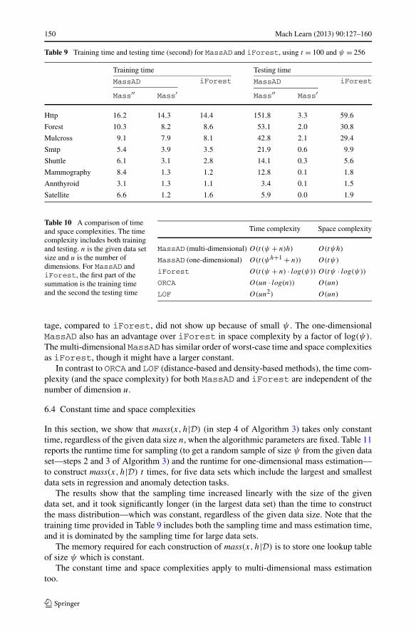
In this section, we show that mass(x,h|D) (in step 4 of Algorithm 3) takes only constanttime, regardless of the given data size n, when the algorithmic parameters are fixed. Table 11reports the runtime time for sampling (to get a random sample of size ψ from the given dataset—steps 2 and 3 of Algorithm 3) and the runtime for one-dimensional mass estimation—to construct mass(x,h|D) t times, for five data sets which include the largest and smallestdata sets in regression and anomaly detection tasks.

The results show that the sampling time increased linearly with the size of the givendata set, and it took significantly longer (in the largest data set) than the time to constructthe mass distribution—which was constant, regardless of the given data size. Note that thetraining time provided in Table 9 includes both the sampling time and mass estimation time,and it is dominated by the sampling time for large data sets.

The memory required for each construction of mass(x,h|D) is to store one lookup tableof size ψ which is constant.

The constant time and space complexities apply to multi-dimensional mass estimationtoo.

Mach Learn (2013) 90:127–160 151

Table 11 Runtime (second) forsampling, mass(x,1|D) andmass(x,3|D), where t = 1000and ψ = 8

Data size Sampling mass(x,1|D) mass(x,3|D)

Http 567497 138.30 0.33 10.96

Shuttle 49097 16.16 0.39 10.97

COREL 10000 1.23 0.27 11.03

tic 9822 1.09 0.43 11.14

concrete 1030 0.18 0.31 10.95

Fig. 9 Runtime comparison:One-dimensional massestimation versusmulti-dimensional massestimation for different values ofh in the COREL data set, whereboth are using ψ = 8 andt = 1000. In this experiment, weset h to the required value formulti-dimensional massestimation, rather than h = ψ

which was used in allexperiments reported in theprevious sections

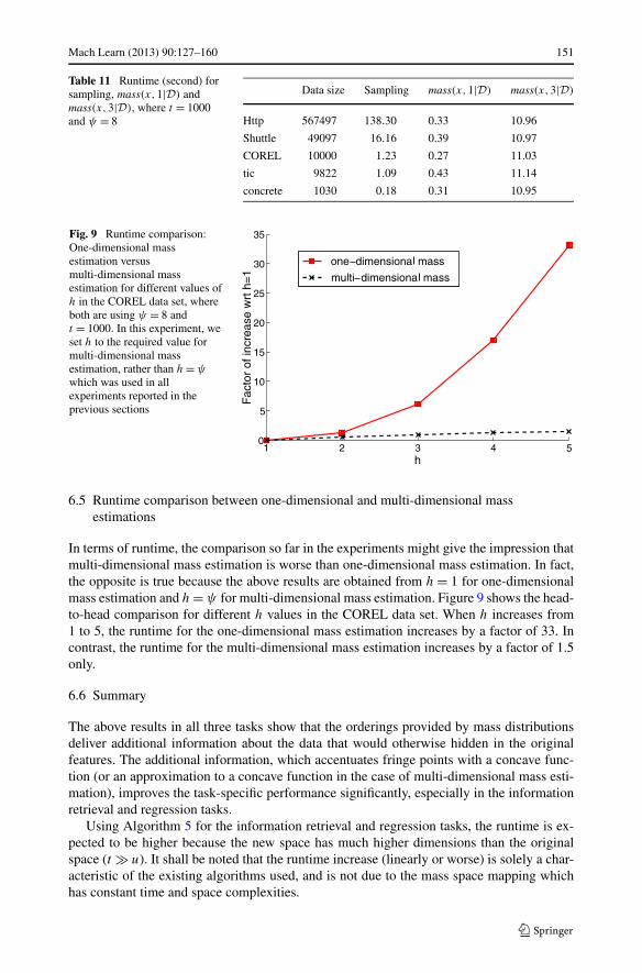
6.5 Runtime comparison between one-dimensional and multi-dimensional massestimations

In terms of runtime, the comparison so far in the experiments might give the impression thatmulti-dimensional mass estimation is worse than one-dimensional mass estimation. In fact,the opposite is true because the above results are obtained from h = 1 for one-dimensionalmass estimation and h = ψ for multi-dimensional mass estimation. Figure 9 shows the head-to-head comparison for different h values in the COREL data set. When h increases from1 to 5, the runtime for the one-dimensional mass estimation increases by a factor of 33. Incontrast, the runtime for the multi-dimensional mass estimation increases by a factor of 1.5only.

6.6 Summary

The above results in all three tasks show that the orderings provided by mass distributionsdeliver additional information about the data that would otherwise hidden in the originalfeatures. The additional information, which accentuates fringe points with a concave func-tion (or an approximation to a concave function in the case of multi-dimensional mass esti-mation), improves the task-specific performance significantly, especially in the informationretrieval and regression tasks.

Using Algorithm 5 for the information retrieval and regression tasks, the runtime is ex-pected to be higher because the new space has much higher dimensions than the originalspace (t � u). It shall be noted that the runtime increase (linearly or worse) is solely a char-acteristic of the existing algorithms used, and is not due to the mass space mapping whichhas constant time and space complexities.

152 Mach Learn (2013) 90:127–160

Table 12 A comparison of kernel density estimation and mass estimation. Kernel density estimation requirestwo parameter settings: kernel function K(·) and bandwidth hw ; mass estimation has one: h

Kernel density(x) = 1nhw

∑ni=1 K(

x−xihw

)

mass(x,h) ={∑n−1

i=1 massi (x,h-1)p(si ), h > 1∑n−1i=1 mi(x)p(si ), h = 1

We believe that a more tailored approach that better integrates the information providedby mass (into the C3 component in the formalism) for a specific task can potentially fur-ther improve the current level of performance in terms of either task-specific performancemeasure or runtime. We have demonstrated this ‘direct’ application using Algorithm 6 forthe anomaly detection task, in which MassAD performs equally well or significantly betterthan four state-of-the-art methods in terms of task-specific performance measure, and theone-dimensional mass estimation executes faster than all other methods in terms of runtime.

Why does one-dimensional mapping work when tackling multi-dimensional problems?We conjecture that if there is no or little interaction between features, then the one-dimensional mapping will work because the ordering that accentuates the fringe pointsfor each original dimension making it easy for existing algorithms to exploit. When thereare strong interactions between features, then one-dimensional mapping might not achievegood results. Indeed, our results in all three tasks show that multi-dimensional mass esti-mation does perform better than one-dimensional mass estimation in general, in terms oftask-specific performance measures.

The ensemble method for mass estimation usually needs only a small sample to buildeach model in an ensemble. In addition, in order to build all t models for an ensemble, tψ

could be more than n when ψ > n/t .The key limitation of the one-dimensional mass estimation is its high cost when a high

value of h is applied. This can be avoided by implementing it using a tree structure ratherthan a lookup table, as we have done using Half-Space Trees which reduces the time com-plexity to O(th(ψ + n)) from O(t(ψh+1 + n)).

7 Relation to kernel density estimation

A comparison of mass estimation and kernel density estimation is provided in Table 12.Like kernel estimation, mass estimation at each point is computed through a summation

of a series of values from a mass base function mi(·), equivalent to a kernel function K(·).The two methods differ in the following ways:

• Aim: Kernel estimation is aimed to do probability density estimation; whereas mass esti-mation is to estimate an order from the core points to the fringe points.

• Kernel function: While kernel estimation can use different kernel functions for probabilitydensity estimation; we doubt that mass estimation requires a different base function fortwo reasons. First, a more sophisticated function is unlikely to provide a better orderingthan a simple rectangular function. Second, the rectangular function keeps the computa-tion simple and fast. In addition, a kernel function must be fixed (i.e., having user-definedvalues for its parameters); e.g., the rectangular kernel function has fixed width or fixed perunit size. But the rectangular function used in mass has no parameter and no fixed width.

• Sample size: Kernel estimation or other density estimation methods require a large samplesize in order to estimate the probability accurately (Duda et al. 2001). Mass estimation

Mach Learn (2013) 90:127–160 153

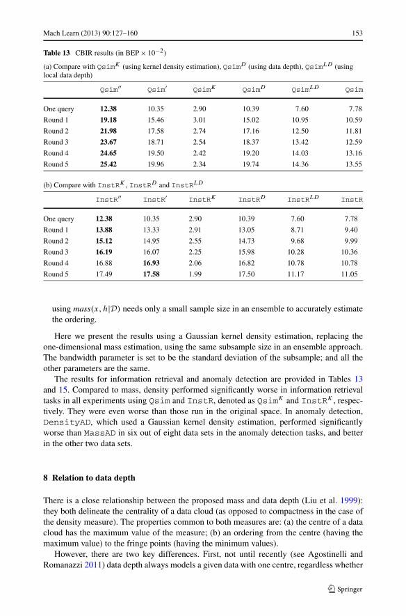
Table 13 CBIR results (in BEP × 10−2)

(a) Compare with QsimK (using kernel density estimation), QsimD (using data depth), QsimLD (usinglocal data depth)

Qsim′′ Qsim′ QsimK QsimD QsimLD Qsim

One query 12.38 10.35 2.90 10.39 7.60 7.78

Round 1 19.18 15.46 3.01 15.02 10.95 10.59

Round 2 21.98 17.58 2.74 17.16 12.50 11.81

Round 3 23.67 18.71 2.54 18.37 13.42 12.59

Round 4 24.65 19.50 2.42 19.20 14.03 13.16

Round 5 25.42 19.96 2.34 19.74 14.36 13.55

(b) Compare with InstRK , InstRD and InstRLD

InstR′′ InstR′ InstRK InstRD InstRLD InstR

One query 12.38 10.35 2.90 10.39 7.60 7.78

Round 1 13.88 13.33 2.91 13.05 8.71 9.40

Round 2 15.12 14.95 2.55 14.73 9.68 9.99

Round 3 16.19 16.07 2.25 15.98 10.28 10.36

Round 4 16.88 16.93 2.06 16.82 10.78 10.78

Round 5 17.49 17.58 1.99 17.50 11.17 11.05

using mass(x,h|D) needs only a small sample size in an ensemble to accurately estimatethe ordering.

Here we present the results using a Gaussian kernel density estimation, replacing theone-dimensional mass estimation, using the same subsample size in an ensemble approach.The bandwidth parameter is set to be the standard deviation of the subsample; and all theother parameters are the same.

The results for information retrieval and anomaly detection are provided in Tables 13and 15. Compared to mass, density performed significantly worse in information retrievaltasks in all experiments using Qsim and InstR, denoted as QsimK and InstRK , respec-tively. They were even worse than those run in the original space. In anomaly detection,DensityAD, which used a Gaussian kernel density estimation, performed significantlyworse than MassAD in six out of eight data sets in the anomaly detection tasks, and betterin the other two data sets.

8 Relation to data depth

There is a close relationship between the proposed mass and data depth (Liu et al. 1999):they both delineate the centrality of a data cloud (as opposed to compactness in the case ofthe density measure). The properties common to both measures are: (a) the centre of a datacloud has the maximum value of the measure; (b) an ordering from the centre (having themaximum value) to the fringe points (having the minimum values).

However, there are two key differences. First, not until recently (see Agostinelli andRomanazzi 2011) data depth always models a given data with one centre, regardless whether

154 Mach Learn (2013) 90:127–160

Table 14 CBIR results (online time cost in seconds)

(a) Compare with QsimK , QsimD , QsimLD

Qsim′′ Qsim′ QsimK QsimD QsimLD Qsim

One query 0.715 0.822 0.820 0.840 0.829 0.093

Round 1 0.207 0.208 0.224 0.237 0.226 0.035

Round 2 0.228 0.231 0.279 0.288 0.276 0.058

Round 3 0.257 0.259 0.348 0.355 0.343 0.086

Round 4 0.291 0.294 0.435 0.438 0.425 0.122

Round 5 0.335 0.341 0.547 0.543 0.531 0.167

(b) Compare with InstRK , InstRD and InstRLD

InstR′′ InstR′ InstRK InstRD InstRLD InstR

One query 0.715 0.822 0.820 0.840 0.829 0.093

Round 1 0.197 0.198 0.203 0.215 0.206 0.026

Round 2 0.200 0.200 0.205 0.216 0.206 0.028

Round 3 0.200 0.200 0.206 0.217 0.207 0.028

Round 4 0.200 0.200 0.207 0.218 0.208 0.028

Round 5 0.200 0.200 0.207 0.218 0.208 0.028

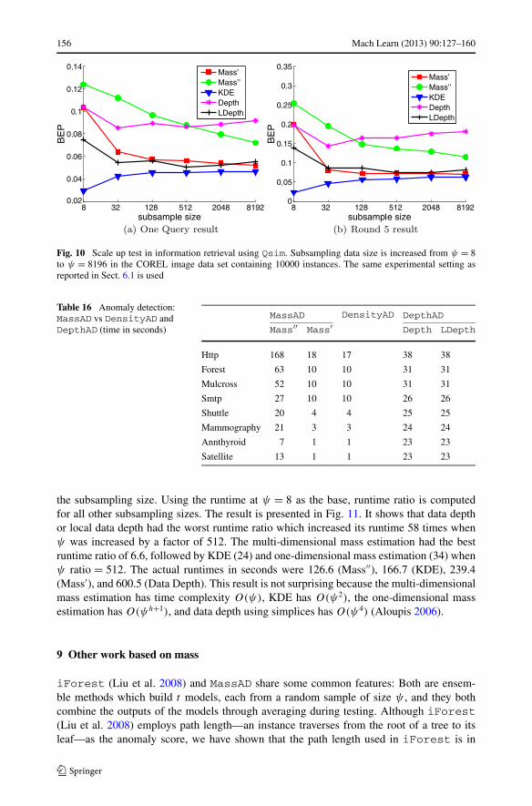
Table 15 Anomaly detection:MassAD vs DensityAD andDepthAD (AUC)

MassAD DensityAD DepthAD

Mass′′ Mass′ Depth LDepth

Http 1.00 1.00 0.99 0.98 0.52

Forest 0.90 0.92 0.70 0.85 0.49

Mulcross 0.26 0.99 1.00 0.99 0.93

Smtp 0.91 0.86 0.59 0.92 0.93

Shuttle 1.00 0.99 0.90 0.87 0.72

Mammography 0.86 0.37 0.27 0.36 0.79

Annthyroid 0.75 0.71 0.80 0.58 0.86

Satellite 0.77 0.62 0.61 0.59 0.69

the data is unimodal or multi-modal; whereas mass can model both unimodal and multi-modal data by setting h = 1 or h > 1. Local data depth (Agostinelli and Romanazzi 2011)has a parameter (τ ) which allows it to model multi-modal data as well as unimodal data.However, the performance of local data depth appears to be sensitive to the setting of τ (seea discussion of the comparison below). In contrast, a single setting of h in mass estimationhad produced good task-specific performance in three different tasks in our experiments.

Second, mass is a simple and straightforward measure, and has efficient estimation meth-ods based on axis-parallel partitions only. Data depth has many different definitions, depend-ing on the construct used to define depth. The constructs could be Mahalanobis, ConvexHull, simplicial, halfspace and so on (Liu et al. 1999), all of which are expensive to compute(Aloupis 2006)—this has been the main obstacle in applying data depth to real applicationsin multi-dimensional problems. For example, Ruts and Rousseeuw (1996) compute the con-tour of data depth of a data cloud for visualization, and employ depth as the anomaly score to

Mach Learn (2013) 90:127–160 155

identify anomalies. Because of its computational cost, it is limited to small data size only. Incontrast to the axis-parallel partitions used in mass estimation, halfspace data depth5 (Tukey1975), for example, requires to consider all halfspaces which demands high computationaltime and space.

To provide a comparison, we replace the one-dimensional mass estimation (definedin Algorithm 3) with data depth (defined by simplicial depth Liu et al. 1999) and localdata depth (defined by simplicial local depth Agostinelli and Romanazzi 2011). We repeatthe experiments by employing both the data depth and local data depth implementationin R by Agostinelli and Romanazzi (2011) (accessible from r-forge.r-project.org/projects/localdepth). Both data depths are carried out in the same approach by using sample sizeψ to build each of the t models in an ensemble.6 The number of simplices used to do theempirical estimation is set to 10000 for all runs. Default settings are used for all other pa-rameters (i.e., the membership of a data point in simplices is evaluated in the “exact” moderather than the approximate mode, and the tolerance parameter is fixed to 10−9). Note thatlocal depth uses an additional parameter τ to select candidate simplices, where a simplexhaving volume larger than τ is excluded from consideration. As the performance of localdepth is sensitive to τ , we employ the quantile order of τ of 10 %, the low value of the range10 %–30 % suggested by Agostinelli and Romanazzi (2011). Because both data depth andlocal data depth are estimated using the same procedure, their runtimes are the same.

The task-specific performance result for information retrieval is provided in Table 13.Note that local data depth could produce worse retrieval results than those in the originalfeature space. Data depth performed close to that achieved by the one-dimensional massestimation, but it was significantly worse than the multi-dimensional mass estimation.

Figure 10 shows a scale up test in the information retrieval task using Qsim with onequery and feedback round 5. It is interesting to note both mass and data depth performedbetter using small rather than large subsampling size. As expected, KDE produced betterresults with increasing subsampling sizes; but even with ψ = 8196 in the COREL data setof 10000 instances, KDE still performed the worst compared to mass and data depth.

Table 15 shows the result in anomaly detection. Data depth performed worse than bothversions of mass estimation in six out of eight data sets; local data depth performed worsethan multi-dimensional mass estimation in five out of eight data sets; local data depth versusone-dimensional mass estimation have four wins and four losses. Note that though local datadepth achieved the best result in two data sets, it also produced the worst in three data setswhich were significantly worse than others (in http, forest and shuttle).

The runtime results are provided in Tables 14 and 16. These results do not reveal the timecomplexities of the algorithms because of small ψ (and the CBIR results do not include theoffline time cost). We conducted a scale up test using the Mulcross data set by increasing

5Zuo and Serfling (2000) define halfspace data depth (HD) of a point x in Ru w.r.t. a probability measure P

on Ru as the minimum probability mass carried by any closed halfspace containing x:

HD(x;P) = inf{P(H) : H a closed halfspace, x ∈ H

}, x ∈ Ru

In the language of data depth, the one-dimensional mass estimation may be interpreted as a kind of averageprobability mass of halfspaces containing x, weighted by mass covered by halfspace. But the one-dimensionalmass estimation defined in (1) allows mass to be computed by a summation of n − 1 components from thegiven data set of size n, whereas data depth does not. In addition, our implementation of multi-dimensionalmass estimation using a tree structure with axis-parallel splits cannot be interpreted using any of the constructsemployed by data depth.6Our experiments indicate that using the entire data set to estimate data depth or local data depth producesworse results than those using an ensemble approach. This result is shown in Appendix.

156 Mach Learn (2013) 90:127–160

Fig. 10 Scale up test in information retrieval using Qsim. Subsampling data size is increased from ψ = 8to ψ = 8196 in the COREL image data set containing 10000 instances. The same experimental setting asreported in Sect. 6.1 is used

Table 16 Anomaly detection:MassAD vs DensityAD andDepthAD (time in seconds)

MassAD DensityAD DepthAD

Mass′′ Mass′ Depth LDepth

Http 168 18 17 38 38

Forest 63 10 10 31 31

Mulcross 52 10 10 31 31

Smtp 27 10 10 26 26

Shuttle 20 4 4 25 25

Mammography 21 3 3 24 24

Annthyroid 7 1 1 23 23

Satellite 13 1 1 23 23

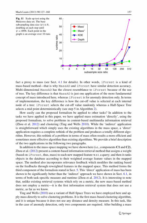
the subsampling size. Using the runtime at ψ = 8 as the base, runtime ratio is computedfor all other subsampling sizes. The result is presented in Fig. 11. It shows that data depthor local data depth had the worst runtime ratio which increased its runtime 58 times whenψ was increased by a factor of 512. The multi-dimensional mass estimation had the bestruntime ratio of 6.6, followed by KDE (24) and one-dimensional mass estimation (34) whenψ ratio = 512. The actual runtimes in seconds were 126.6 (Mass′′), 166.7 (KDE), 239.4(Mass′), and 600.5 (Data Depth). This result is not surprising because the multi-dimensionalmass estimation has time complexity O(ψ), KDE has O(ψ2), the one-dimensional massestimation has O(ψh+1), and data depth using simplices has O(ψ4) (Aloupis 2006).

9 Other work based on mass

iForest (Liu et al. 2008) and MassAD share some common features: Both are ensem-ble methods which build t models, each from a random sample of size ψ , and they bothcombine the outputs of the models through averaging during testing. Although iForest(Liu et al. 2008) employs path length—an instance traverses from the root of a tree to itsleaf—as the anomaly score, we have shown that the path length used in iForest is in

Mach Learn (2013) 90:127–160 157

Fig. 11 Scale up test using theMulcross data set. The basesubsampling data size (ψ ) is 8;doubling at each step untilψ = 4096. Each point in thegraph is an average over 10 runs

fact a proxy to mass (see Sect. 4.1 for details). In other words, iForest is a kind ofmass-based method—that is why MassAD and iForest have similar detection accuracy.Multi-dimensional MassAD has the closest resemblance to iForest because of the useof tree. The key difference is that MassAD is just one application of the more fundamentalconcept of mass introduced here, whereas iForest is for anomaly detection only. In termsof implementation, the key difference is how the cut-off value is selected at each internalnode of a tree: iForest selects the cut-off value randomly whereas a Half-Space Treeselects a mid point deterministically (see step 5 in Algorithm 2).

How easily can the proposed formalism be applied to other tasks? In addition to thetasks we have applied in this paper, we have applied mass estimation ‘directly’, using theproposed formalism, to solve problems in content-based multimedia information retrieval(Zhou et al. 2012) and clustering (Ting and Wells 2010). While the ‘indirect’ applicationis straightforward which simply uses the existing algorithms in the mass space, a ‘direct’application requires a complete rethink of the problem and produces a totally different algo-rithm. However, this rethink of a problem in terms of mass often results a more efficient andsometimes more effective algorithm than existing algorithms. We provide a brief descriptionof the two applications in the following two paragraphs.

In addition to the mass-space mapping we have shown here (i.e., components C1 and C2),Zhou et al. (2012) present a content-based information retrieval method that assigns a weight(based on iForest, thus, mass) to each new mapped feature w.r.t. a query; and then it ranksobjects in the database according to their weighted average feature values in the mappedspace. The method also incorporates relevance feedback which modifies the ranking basedon the feedbacks through reweighted features in the mapped space. This method forms thethird component of the formalism stated in Sect. 5. This ‘direct’ application of mass has beenshown to be significantly better than the ‘indirect’ approach we have shown in Sect. 6.1, interms of both task-specific measure and runtime (Zhou et al. 2012). It is interesting to notethat, unlike existing retrieval systems which rely on a metric, the new mass-based methoddoes not employ a metric—it is the first information retrieval system that does not use ametric, as far as we know.

Ting and Wells (2010) use a variant of Half-Space Trees we have employed here and ap-ply mass directly to solve clustering problems. It is the first mass-based clustering algorithm,and it is unique because it does not use any distance and density measure. In this task, likein the case of anomaly detection, only two components are required. After building a mass

158 Mach Learn (2013) 90:127–160

model (in the C1 component), the C3 component consists of linking instances with non-zero mass connected by the mass model and making each group of connected instances aseparate cluster; and all other unconnected instances are regarded as noise. This mass-basedclustering algorithm has been shown to perform equally well as DBSCAN (Ester et al. 1996)in terms of clustering performance, but it runs orders of magnitude faster (Ting and Wells2010).

The earlier version of this paper (Ting et al. 2010) establishes the properties of mass esti-mation in the one-dimensional setting only; and use it in all three tasks. This paper extendsone-dimensional mass estimation to multi-dimensional mass estimation using the same ap-proach as described by Ting and Wells (2010), and implements multi-dimensional massestimation using Half-Space Trees. This paper reports new experiments using the multi-dimensional mass estimation, and shows the advantage of using multi-dimensional massestimation over one-dimensional mass estimation in the three tasks reported earlier (Tinget al. 2010). These related works show that mass estimation can be implemented in differentways using tree-based or non-tree-based methods.

10 Conclusions and future work

This paper makes two key contributions. First, we introduce a base measure, mass, anddelineate its three properties: (i) a mass distribution stipulates an ordering from core pointsto fringe points in a data cloud; (ii) this ordering accentuates the fringe points with a concavefunction—a property that can be easily exploited by existing algorithms to improve theirtask-specific performance; and (iii) the mass estimation methods have constant time andspace complexities. Density estimation has been the base modelling mechanism employedin many techniques thus far. Mass estimation introduced here provides an alternative choice,and it is better suited for many tasks which require an ordering rather than probability densityestimation.

Second, we present a mass-based formalism which forms a basis to apply mass to dif-ferent tasks. The three tasks (i.e., information retrieval, regression and anomaly detection)to which we have successfully applied are just examples of its application. Mass estimationhas potentials in many other applications.

There are potential extensions to the current work. First, the algorithms for the threetasks and the formalism can be improved or extended to include more tasks. Second, be-cause the purposes and their properties differ, mass estimation is not intended to replacedensity estimation—it is thus important to identify areas in which each is best suited for.This will ascertain (i) areas in which density has been a mismatch, unbeknown up to now,and (ii) areas in which mass estimation is weak. Third, the proposed approach to multi-dimensional mass estimation is an approximation and it does not guarantee concavity. Itwill be interesting to explore a version that has such a guarantee and to examine whether itwill further improve the task-specific performance in all three tasks reported here. Fourth,the current implementation of multi-dimensional mass estimation using Half-Space Treeslimits its applications to low dimensional problems because it suffers the same problem as inall other grid oriented methods. We will explore non-grid oriented implementations of masswhich have potential to tackle high dimensional problems more effectively than existingdensity-based and distance-based methods.

The Matlab source codes of both one-dimensional and multi-dimensional massestimations are available at http://sourceforge.net/projects/mass-estimation/.

Mach Learn (2013) 90:127–160 159

Acknowledgements This work is supported by the Air Force Research Laboratory, under agreement num-bers FA2386-09-1-4014, FA2386-10-1-4052 and FA2386-11-1-4112. The US Government is authorized toreproduce and distribute reprints for Governmental purposes notwithstanding any copyright notation thereon.The anonymous reviewers have provided many helpful comments to improve the clarity of this paper.

Appendix: Anomaly detection using data depth that builds a single model from theentire data set

This appendix provides the results in anomaly detection task where data depth and localdata depth built a single model from the entire data set, i.e., DepthADs . This is in contrastto DepthAD which employed an ensemble approach in Sect. 8.

Table 17 shows that MassAD generally has higher AUC than DepthADs which em-ployed either data depth or local data depth. The only exception is the Annthyroid data set.Note that these results are generally worse than those employing an ensemble approach,reported in Table 15.

Table 17 AUC values foranomaly detection, comparingMassAD with DepthADs

(which employed either datadepth or local data depth) thatbuild a single model from theentire data set

MassAD DepthADs

Mass′′ Mass′ Depth LDepth

Http 1.00 1.00 0.84 0.50

Forest 0.90 0.92 0.50 0.55

Mulcross 0.26 0.99 0.88 0.61

Smtp 0.91 0.86 0.86 0.76

Shuttle 1.00 0.99 0.51 0.70

Mammography 0.86 0.37 0.73 0.62

Annthyroid 0.75 0.71 0.59 0.85

Satellite 0.77 0.62 0.50 0.70

References

Achtert, E., Kriegel, H.-P., & Zimek, A. (2008). ELKI: a software system for evaluation of subspace clusteringalgorithms. In Proceedings of the 20th international conference on scientific and statistical databasemanagement (pp. 580–585).

Agostinelli, C., & Romanazzi, M. (2011). Local depth. Journal of Statistical Planning and Inference, 141,817–830.

Aloupis, G. (2006). Geometric measures of data depth. DIMACS Series in Discrete Math and TheoreticalComputer Science, 72, 147–158.

Asuncion, A., & Newman, D. (2007). UCI machine learning repository.Bay, S. D., & Schwabacher, M. (2003). Mining distance-based outliers in near linear time with randomization

and a simple pruning rule. In Proceedings of ACM SIGKDD (pp. 29–38).Breunig, M. M., Kriegel, H.-P., Ng, R. T., & Sander, J. (2000). LOF: identifying density-based local outliers.

In Proceedings of ACM SIGKDD (pp. 93–104).Chang, C.-C., & Lin, C.-J. (2001). LIBSVM: a library for support vector machines.Duda, R., Hart, P., & Stork, D. (2001). Pattern classification (2nd ed.). New York: Wiley.Ester, M., Kriegel, H.-P., Sander, J., & Xu, X. (1996). A density-based algorithm for discovering clusters in

large spatial databases with noise. In Proceedings of ACM SIGKDD (pp. 226–231).Giacinto, G., & Roli, F. (2005). Instance-based relevance feedback for image retrieval. In Advances in NIPS

(pp. 489–496).

160 Mach Learn (2013) 90:127–160

He, J., Li, M., Zhang, H., Tong, H., & Zhang, C. (2004). Manifold-ranking based image retrieval. In Proceed-ings of ACM multimedia (pp. 9–16).

Liu, F. T., Ting, K. M., & Zhou, Z.-H. (2008). Isolation forest. In Proceedings of IEEE ICDM (pp. 413–422).Liu, R., Parelius, J. M., & Singh, K. (1999). Multivariate analysis by data depth. The Annals of Statistics,

27(3), 783–840.Quinlan, J. (1993). C4.5: programs for machine learning. San Mateo: Morgan Kaufmann.Rocke, D. M., & Woodruff, D. L. (1996). Identification of outliers in multivariate data. Journal of the Ameri-

can Statistical Association, 91(435), 1047–1061.Ruts, I., & Rousseeuw, P. (1996). Computing depth contours of bivariate point clouds. Computational Statis-

tics and Data Analysis, 23(1), 153–168.Schölkopf, B., Williamson, R. C., Smola, A. J., Shawe-Taylor, J., & Platt, J. C. (2000). Support vector method

for novelty detection. In Advances in NIPS (pp. 582–588).Simonoff, J. S. (1996). Smoothing methods in statistics. Berlin: Springer.Ting, K. M., & Wells, J. R. (2010). Multi-dimensional mass estimation and mass-based clustering. In Pro-

ceedings of IEEE ICDM (pp. 511–520).Ting, K. M., Zhou, G.-T., Liu, F. T., & Tan, S. C. (2010). Mass estimation and its applications. In Proceedings

of ACM SIGKDD (pp. 989–998).Tukey, J. W. (1975). Mathematics and picturing data. In Proceedings of the international congress on math-

ematics (Vol. 2, pp. 525–531).Vapnik, V. N. (2000). The nature of statistical learning theory (2nd ed.). Berlin: Springer.Zhang, R., & Zhang, Z. (2006). BALAS: empirical Bayesian learning in the relevance feedback for image

retrieval. Image and Vision Computing, 24(3), 211–223.Zhou, G.-T., Ting, K. M., Liu, F. T., & Yin, Y. (2012). Relevance feature mapping for content-based multi-

media information retrieval. Pattern Recognition, 45, 1707–1720.Zhou, Z.-H., Chen, K.-J., & Dai, H.-B. (2006). Enhancing relevance feedback in image retrieval using unla-

beled data. ACM Transactions on Information Systems, 24(2), 219–244.Zhou, Z.-H., & Dai, H.-B. (2006). Query-sensitive similarity measure for content-based image retrieval. In

Proceedings of IEEE ICDM (pp. 1211–1215).Zuo, Y., & Serfling, R. (2000). General notion of statistical depth function. The Annal of Statistics, 28, 461–

482.