MASS BALANCING –MIDAS APPROACH

Metallurgical Accounting Course, South Africa 2015

MIDASTech International

THE ADVANTAGES OF DETAILED MASS BALANCE

• Units process particles

• So understanding the complex response of particles to units processes facilitates the basis of accurate simulation; rather than fictional simulation which is all too common.

• Metallurgical accounting focuses on assays, and is therefore a 1D Balance and inappropriate for simulation or understanding metallurgical processing of the ore

MASS BALANCING LEVELS

• 0D Balance – Solid flows and Water flows

• 1D Balance - Size, OR bulk assays, OR elements OR density classes OR Minerals

• 2D Balance i.e. Size/assay

• 3D Balance Size, Particle Types (i.e. density class), Properties of particle types (i.e. multimineral composition)

MIDASTech International

DATA STRUCTURES FOR MASS BALANCING

THE VARIOUS LEVELS OF MASS BALANCING

• The diagram shows the general structure of ore information. Measurement of information and structure are not the same.

• A poorly constructed simulator will be based on measurable information only rather than the actual ore structure.

• An intelligent simulator will use the measured information to identify the actual ore properties.

LEVELS OF MASS BALANCING CONTINUED

• Hence it is not necessarily required to obtain the detail information (3D); only to infer it from the 2D information. Hence there is a hierarchical approach to mass balancing. Generally 1D first to ensure solid flows are estimated; then 2D to ensure general mass balance consistency.

• The 2D information can actually be used to infer the 3D, which is also mass balanced, but not necessarily based on 3D measurement. On the other hand a user can directly measure 3D data via float-sink tests – and then elemental composition in each density class, or mineralogical analysis.

• However the fundamental object remains – to identify the flow of particles through the circuit

ACTUAL MINERAL PROCESSING DATA

STRUCTURE• Particles are multimineral

MULTIMINERAL PARTICLES

• The figure shows a multimineral particle.

• It is self-evident from examining ore particles that they are indeed multimineral.

• The important concept is that one would think that if we were to model multimineral particles in mineral processing we would need billions of particles. But we don’t!

• We are only seeking a representative set of multimineral particles, say 200 per size-class which can easily be handled by simple calculation software such as Excel.

PARTICLE RECOVERY

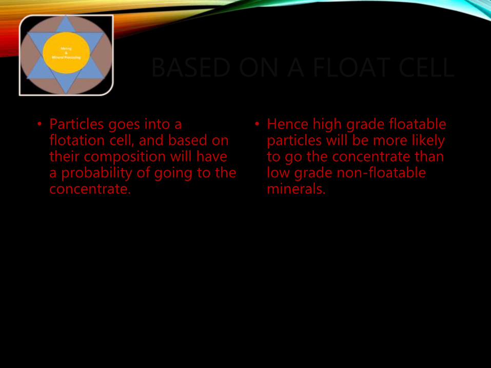
BASED ON A FLOAT CELL

• Particles goes into a flotation cell, and based on their composition will have a probability of going to the concentrate.

• Hence high grade floatable particles will be more likely to go the concentrate than low grade non-floatable minerals.

PARTITION CURVES FOR UNDERSTANDING EFFICIENCY

Mineral Composition

Probability of particle going to concentrate

Inefficient

Efficient

FROM THE PREVIOUS DIAGRAM

• So if we know the information about particle distributions before and after a flotation cell, we can plot the ‘partition curve’ – the probability a particle of a particular grade will go to the concentrate.

• It is not enough to know assays before and after a float cell, as it can be affected by the distribution of mineral in the particles. Hence the partition curve helps us to distinguish units that are performing efficiently from those that are performing inefficiently.

COMPOSITION OF A MINERAL IS INSUFFICIENT TO DEVELOP

A MODEL

Two particles both with the same composition of valuable mineral (say chalcopyrite). In a simple model they would be presumed to have the same properties

LOOKING AT MINERAL PARTICLES…

• But looking at the mineral composition of just one mineral is not good enough!

• Here we see two particles – both have the same grade of valuable mineral interest. All other minerals are combined to form the respective ‘gangue’ mineral. An inexperienced metallurgist would think that the two particles have the same properties and therefore should float the same.

• But if you think a little bit deeper, you might want to think about the ‘gangue’ phase

LOOK A BIT DEEPER

The gangue mineral may be different i.e. quartz for particle 1 and pyrite for particle 2. The belief the two particles will have the same properties (particularly in flotation) is at best a work of fiction. Clearly we need to recognise the existence of multiminerals

FAILURE TO RECOGNISE THE EXISTENCE OF MULTIPLE

MINERALS• Impractical models• Fictional models• Inordinate amount of laboratory analysis• Lack of trust in simulation• Invalid assay to mineral algorithms• General confusion

BENEFITS OF DETAILED MODELLING

• One can identify whether units are performing efficiently for a given ore type

• Essential for plant trouble shooting

• Essential for plant simulation

• Essential for identifying how operational changes affect final grades and recoveries

• Use of multiple mineral particles is essential for accuracy of models –particularly separation of associated minerals such as pyrite, chalcopyrite

THE SOLUTION!

• Recognise the existence of multiminerals (where they exist)

• Use software that incorporates modern mathematical methods to deal with the real datastructure (Advanced simulation course, inclusive of advanced mass balancing methods)

• Such methods are only available through MIDASTech

QUANTITATIVE ADVANTAGES

• The MIDAS approach (Mass balancing together with simulation ) would target 5% operational improvement

• Leading to millions of dollars of savings per plant.

MIDAS TECH’S SET OF MASS BALANCE SYSTEMS

• 1. MMVisioBal1D – 1D Mass Balance system,

• 2. MMVisioBal2D – 2D Mass Balance system,

• 3. MMVisioBal3D – 3D Mass Balance system

• 4. MMVisioBal2DPlus - inferring detailed 3D information from 2D data (patented approach)

MASS BALANCING METHODS

Two main approaches of mass balancing

• Conventional: Least squares – requires variances of estimates; and is therefore a flawed approach if variances are not known

• Modern: Information theory – appropriate when variances are known; and can also be used when variances are known. Fast, efficient and allows inference (MMVisioBalPlus)

MMVISIOBAL1D

• Entry point software (contact Stephen@MIDASTech.net)

• Uses Visio flowsheet system and Excel interface. System largely automated. Once an Excel template is created and data are inputted – press of a button yields mass balance results

VISIO FLOWSHEET

Balanced

Variable

Stream

S1 S2 S3 S4 S8 S13 S11 S6 S17 S20 S23 S25 S27 S16 S19 S22 S5

TotalFlow

PercentSolids

SolidFlow 99695.00 105.01 74.85 99514.86 99315.01 99160.55 154.46 259.58 0.14 0.49 211.94 152.39 60.19 104.86 74.36 354.49 99575.05

WaterFlow

Assay

Au 1.21 26.90 32.17 1.15 1.06 1.03 19.28 38.04 19.28 20.23 13.99 18.19 3.43 26.90 32.25 35.71 1.16

Ag 33.97 1577.80 1752.46 31.04 27.60 26.21 915.26 1352.55 1288.41 1235.70 631.45 843.08 100.56 1577.61 1755.20 1374.14 31.08

Cu 1.30 17.50 15.15 1.27 1.24 1.22 12.82 13.01 21.73 14.14 9.97 12.73 3.05 17.49 15.16 14.63 1.27

Pb 1.21 4.81 4.52 1.20 1.19 1.18 4.82 5.25 5.20 4.02 2.43 3.00 1.01 4.81 4.52 5.78 1.20

F 779.56 1469.01 1520.43 778.20 777.52 777.14 1025.34 1101.44 1071.12 1402.03 1300.17 1313.65 1265.59 1469.47 1521.11 1040.69 778.49

Remainder 97.42 77.38 79.99 97.45 97.49 97.52 82.16 81.49 72.84 81.57 87.40 84.05 95.80 77.39 79.98 79.35 97.45

SIMPLE EXCEL INTERFACE

False Specification

Project Name MMMichaud

False SubProjectID 1

False False False False

9. Options

Full 2D Full 2D

Water Balance FALSE

Start Experimental

EXPERIMENTAL DATA (MMVISIOBAL1D)

Experimental

Variable

Stream

S1 S2 S3 S4 S8 S13 S11 S6 S17 S20 S23 S25 S27 S16 S19 S22 S5

TotalFlow

PercentSolids 28.60 19.85 16.09 28.12 23.96 24.14 10.65 11.51 4.77 4.01 4.21 19.38 3.65 5.28 7.73 18.00 19.22

SolidFlow 100000 104 74 172 288 142 47

WaterFlow

Assay

Au 1.37 33.78 25.07 1.16 0.59 0.54 6.20 6.85 8.58 14.23 13.90 18.26 6.93 19.33 37.36 53.85 3.43

Ag 60.00 1363.75 1118.75 30.00 22.50 13.75 312.50 377.50 507.50 646.25 557.50 952.50 320.00 1062.50 1601.25 1950.00 42.50

Cu 1.58 19.09 11.97 1.00 1.30 1.00 6.02 6.45 9.17 8.08 9.28 13.65 5.86 13.57 16.25 23.53 1.54

Pb 1.47 5.94 3.55 1.16 1.12 1.07 2.28 2.35 2.24 2.67 2.88 2.53 2.05 3.28 4.86 10.18 1.19

F 868.00 1189.20 1587.20 768.00 786.40 715.80 1190.80 1297.20 1514.60 1507.60 1256.20 1356.20 1223.00 1676.00 1346.00 762.40 759.20

Remainder 96.86 74.71 84.21 97.76 97.49 97.86 91.54 91.04 88.40 89.03 87.66 83.59 91.93 82.87 78.60 66.02 97.18536

CONFIDENCE

Confidence

Variable

Stream

S1 S2 S3 S4 S8 S13 S11 S6 S17 S20 S23 S25 S27 S16 S19 S22 S5

TotalFlow Not Used Not Used Not Used Not Used Not Used Not Used Not Used Not Used Not Used Not Used Not Used Not Used Not Used Not Used Not Used Not Used Not Used

PercentSolids Not Used Not Used Not Used Not Used Not Used Not Used Not Used Not Used Not Used Not Used Not Used Not Used Not Used Not Used Not Used Not Used Not Used

SolidFlow Standard Standard Standard Missing Missing Missing Standard Standard Missing Missing Missing Standard Standard Missing Missing Missing Missing

WaterFlow Not Used Not Used Not Used Not Used Not Used Not Used Not Used Not Used Not Used Not Used Not Used Not Used Not Used Not Used Not Used Not Used Not Used

Assay

Au Standard Standard Standard Standard Standard Standard Standard Standard Standard Standard Standard Standard Standard Standard Standard Standard Standard

Ag Standard Standard Standard Standard Standard Standard Standard Standard Standard Standard Standard Standard Standard Standard Standard Standard Standard

Cu Standard Standard Standard Standard Standard Standard Standard Standard Standard Standard Standard Standard Standard Standard Standard Standard Standard

Pb Standard Standard Standard Standard Standard Standard Standard Standard Standard Standard Standard Standard Standard Standard Standard Standard Standard

F Standard Standard Standard Standard Standard Standard Standard Standard Standard Standard Standard Standard Standard Standard Standard Standard Standard

Remainder Standard Standard Standard Standard Standard Standard Standard Standard Standard Standard Standard Standard Standard Standard Standard Standard Standard

BALANCED

Balanced

Variable

Stream

S1 S2 S3 S4 S8 S13 S11 S6 S17 S20 S23 S25 S27 S16 S19 S22 S5

TotalFlow

PercentSolids

SolidFlow 99695.00 105.01 74.85 99514.86 99315.01 99160.55 154.46 259.58 0.14 0.49 211.94 152.39 60.19 104.86 74.36 354.49 99575.05

WaterFlow

Assay

Au 1.21 26.90 32.17 1.15 1.06 1.03 19.28 38.04 19.28 20.23 13.99 18.19 3.43 26.90 32.25 35.71 1.16

Ag 33.97 1577.80 1752.46 31.04 27.60 26.21 915.26 1352.55 1288.41 1235.70 631.45 843.08 100.56 1577.61 1755.20 1374.14 31.08

Cu 1.30 17.50 15.15 1.27 1.24 1.22 12.82 13.01 21.73 14.14 9.97 12.73 3.05 17.49 15.16 14.63 1.27

Pb 1.21 4.81 4.52 1.20 1.19 1.18 4.82 5.25 5.20 4.02 2.43 3.00 1.01 4.81 4.52 5.78 1.20

F 779.56 1469.01 1520.43 778.20 777.52 777.14 1025.34 1101.44 1071.12 1402.03 1300.17 1313.65 1265.59 1469.47 1521.11 1040.69 778.49

Remainder 97.42 77.38 79.99 97.45 97.49 97.52 82.16 81.49 72.84 81.57 87.40 84.05 95.80 77.39 79.98 79.35 97.45

MMVISIOBAL3D

• Only used by sophisticated Mining Companies that are focused on technically-enable profit strategies

Example:

EXPERIMENTAL

ExperimentalSolidFlow 32.04

SizeDensity

Class Mass%

Elements

Fe SiO2 Al2O3 P S TiO2 Mn CaO MgO LOI Remainder

-6+2 +4.05 13.93 66.33 1.27 0.86 0.07 0.01 0.04 0.02 0.02 0.03 2.36 28.99

+3.6-4.05 21.25 62.09 2.53 2.16 0.15 0.02 0.06 0.03 0.03 0.04 5.76 27.13

+3.3-3.6 16.32 56.05 4.24 4.13 0.21 0.03 0.11 0.05 0.04 0.07 9.84 25.23

+2.85-3.3 8.92 50.90 7.81 7.07 0.18 0.04 0.20 0.04 0.05 0.10 11.25 22.36

+2.6-2.85 2.10 38.39 16.98 14.59 0.11 0.03 0.33 0.04 0.07 0.12 12.22 17.12

-2.6 1.93 24.23 26.92 23.89 0.08 0.03 0.47 0.02 0.12 0.16 13.50 10.58

Average 64.45 58.42 4.36 4.04 0.15 0.02 0.10 0.04 0.04 0.06 7.15 25.62

-2+1 +4.05 10.20 66.21 1.41 0.91 0.07 0.01 0.04 0.02 0.02 0.03 2.39 28.89

+3.6-4.05 6.94 61.06 2.60 2.30 0.17 0.03 0.07 0.05 0.03 0.05 7.06 26.58

+3.3-3.6 11.81 56.71 4.30 4.12 0.20 0.03 0.13 0.05 0.05 0.07 9.67 24.67

+2.85-3.3 5.02 49.82 8.91 7.63 0.16 0.04 0.23 0.04 0.07 0.10 11.30 21.70

+2.6-2.85 1.15 29.80 24.09 19.46 0.10 0.04 0.37 0.02 0.12 0.16 12.67 13.17

-2.6 0.43 13.68 32.28 31.64 0.05 0.04 0.41 0.01 0.08 0.15 15.23 6.43

Average 35.55 58.32 4.54 4.13 0.14 0.02 0.11 0.04 0.04 0.06 7.25 25.33

BALANCED

BalancedSolidFlow

SizeDensity

Class Mass%

Elements

Fe SiO2 Al2O3 P S TiO2 Mn CaO MgO LOI Remainder

-6+2 +4.05 14.44 66.36 1.32 0.94 0.07 0.01 0.04 0.02 0.02 0.04 2.42 28.75

+3.6-4.05 20.34 62.18 2.40 2.16 0.15 0.02 0.05 0.03 0.03 0.04 5.81 27.14

+3.3-3.6 17.21 56.63 4.04 4.07 0.21 0.03 0.11 0.06 0.04 0.07 9.51 25.23

+2.85-3.3 8.58 51.56 7.35 6.87 0.18 0.04 0.18 0.04 0.06 0.10 10.99 22.64

+2.6-2.85 2.21 38.97 16.36 14.68 0.12 0.03 0.31 0.03 0.09 0.13 12.08 17.22

-2.6 1.66 23.48 26.56 24.95 0.07 0.03 0.44 0.03 0.10 0.16 13.75 10.44

Average 64.45 58.42 4.36 4.04 0.15 0.02 0.10 0.04 0.04 0.06 7.15 25.62

-2+1 +4.05 10.30 66.41 1.36 0.91 0.07 0.01 0.04 0.02 0.02 0.03 2.36 28.77

+3.6-4.05 7.83 61.37 2.50 2.30 0.17 0.02 0.07 0.04 0.03 0.05 6.82 26.63

+3.3-3.6 11.43 56.70 4.26 4.21 0.20 0.03 0.13 0.05 0.05 0.07 9.61 24.70

+2.85-3.3 4.51 50.01 8.81 7.77 0.16 0.03 0.22 0.04 0.07 0.11 11.13 21.65

+2.6-2.85 0.86 31.10 22.85 19.08 0.10 0.03 0.34 0.02 0.13 0.15 12.47 13.72

-2.6 0.62 13.51 32.02 32.29 0.05 0.03 0.41 0.01 0.09 0.16 15.11 6.31

Average 35.55 58.32 4.54 4.13 0.14 0.02 0.11 0.04 0.04 0.06 7.25 25.33

Bulk - - 58.39 4.42 4.07 0.15 0.02 0.10 0.04 0.04 0.06 7.19 25.52

INTEGRATED SOFTWARE

• All software, including simulation are integrated into a system called MMPlantMonitor.

• A course (Advanced Simulation) is available. Next scheduled course in South Africa in November via MEI (Flotation 15)

• Stephen Gay Stephen@MIDASTech.net

MIDASTech International