masaryk university...masaryk university faculty of science department of theoretical physics and...
TRANSCRIPT

Masaryk University
Faculty of Science
Department of Theoretical Physics andAstrophysics
Ph.D.Dissertation
Transiting extrasolar planetsand star–planet interaction
Tereza Krejcova
Supervisor: RNDr. Jan Budaj, CSc.
Brno 2013

Bibliographi entryAuthor: Tereza Krejcova
Faculty of Science, Masaryk University
Department of Theoretical Physics and Astrophysics
Title of Dissertation: Transiting extrasolar planets
and star–planet interaction
Degree Programme: Physics
Field of Study: Theoretical Physics and Astrophysics
Supervisor: RNDr. Jan Budaj, CSc.
Astronomical Institute of Slovak Academy of Sciences
Tatranska Lomnica, Slovakia
Academic Year: 2012/2013
Number of Pages: 118
Keywords: Extrasolar planet; light curve; transit; CCD photometry;
out-of-eclipse variation; reflection effect; star–planet interaction;
Ca IIH and K line; logR′
HK parameter; statistical test

Bibliografi k�y z�aznamAutorka: Tereza Krejcova
Prırodovedecka fakulta, Masarykova Univerzita
Ustav Teoreticke Fyziky a Astrofyziky
Nazev prace: Tranzitujıcı extrasolarnı planety
a interakce mezi hvezdou a planetou
Studijnı program: Fyzika
Studijnı obor: Teoreticka Fyzika a Astrofyzika
Skolitel: RNDr. Jan Budaj, CSc.
Astronomicky Ustav Slovenskej Akademie Vied
Tatranska Lomnica, Slovensko
Akademicky rok: 2012/2013
Pocet stran: 118
Klıcova slova: Extrasolarnı planeta; svetelna krivka; tranzit; CCD fotometrie;
mimozakrytove variace; reflexnı jev; interakce hvezda-planeta;
cara Ca IIH a K; parametr logR′
HK; statisticky test

Abstra tThe focus of this thesis is extrasolar planets. The first chapter is devoted to the analysis
of transiting exoplanet light curves and the process followed to determine the physical
and orbital parameters of the system from its measured light curve. In the first sections
of Chapter 1, we describe observations and consequent data analysis of exoplanetary
systems Wasp-10 and TrES-3. Two different telescopes were used, the 50 cm telescope,
located at Stara Lesna, Slovakia and the 2.2m telescope, located at the Calar Alto
Observatory in Spain. The last section of the first chapter is focused on the modelling
of the out-of-eclipse light curve of exoplanetary system KOI-13.01. The changes in this
part of the light curve are extremely small and are caused by a combination of several
effects, such as the reflection of the light from the exoplanet and its dependence on the
phase angle, ellipsoidal variations of the star, the thermal emission from the planet, and
the doppler boosting effect. Such variations in the light curve require a very precise
photometry and are observable from the space only. Data from the Kepler Mission
were used for the verification of the model of the out-of-eclipse light curve. As a result,
the constraints on the Bond albedo of the exoplanet and on the heat redistribution
over the planetary surface were set.
In the second chapter the interaction between the star and exoplanet is studied.
Exoplanets orbiting close enough to their parent stars – in tenths of an astronomical
unit – can interact with the upper layers of their stars’ atmospheres via tidal or magnetic
interaction. We search for the imprints that these effects can leave in the cores of
Ca IIH and K absorption lines, which are formed in the chromosphere of the star.
We studied the correlations between the chromospheric activity represented by two
different indicators – the equivalent width of the core of Ca IIK line and the logR′
HK
parameter – and selected parameters of the star-exoplanet systems, mainly semi-major
axis, planetary mass, and stellar temperature. The sample consists of more than 200
stars with exoplanets. For this purpose the spectra from the Keck HIRES archive and
data obtained with the 2.2m telescope of the European Southern Observatory at La
Silla in Chile were used. We found a statistically significant evidence, that cool stars
(Teff < 5500K) with close-in exoplanets (a < 0.15AU) are more chromosphericaly
active than stars with exoplanets at more distant orbits.

AbstraktTato dizertacnı prace se zabyva studiem extrasolarnıch planet. Prvnı cast se venuje
analyze svetelnych krivek tranzitujıcıch exoplanet. Je zde popsan postup pro zıskanı
fyzikalnıch a orbitalnıch parametru exoplanety z namerenych dat, v tomto prıpade z po-
zorovanych tranzitu dvou exoplanetarnıch systemu Wasp-10 a TrES-3. Zpracovana jsou
zde fotometricka data ze dvou rozdılnych prıstroju – 50 cm dalekohledu ve Stare Lesne
na Slovensku a z 2.2m dalekohledu na observatori Calar Alto ve Spanelsku. Poslednı
sekce prvnı kapitoly se zabyva modelovanım casti svetelne krivky mezi primarnım a
sekundarnım zakrytem exoplanetarnıho systemu KOI-13.01. Zmeny teto casti krivky
ktere jsou extremne male, jsou zpusobeny kombinacı vıce faktoru, jako jsou svetelne
zmeny zpusobene odrazem svetla z hvezdy od planety, elipsoidalnımi variacemi hvezdy,
tepelnym zarenım planety a tzv. “boosting” jevem. Ke studiu takovychto variacı svetelne
krivky jsou zapotrebı presna fotometricka data dosazitelna pouze z vesmıru. Pro overenı
modelu svetelnych zmen mimo primarnı a sekundarnı tranzit jsou proto pouzita data
z druzice Kepler. Vysledkem je urcenı rozmezı hodnot Bondova albeda planety a
ucinnosti prenosu tepla po povrchu planety.
Druha kapitola teto prace je venovana interakci mezi hvezdou a planetou. Predpo-
klada se, ze exoplanety obıhajıcı hvezdu ve velmi male vzdalenosti – radove desetiny as-
tronomicke jednotky –mohou dıky slapove nebo magneticke interakci ovlivnovat vrchnı
vrstvy atmosfery hvezdy. Zamerili jsme se na vyzkum jadra car Ca IIH a K, ktere se for-
mujı ve chromosfere a mohou byt temito efekty ovlivneny. Hledali jsme vzajemnou sou-
vislost mezi chromosferickou aktivitou hvezdy popsanou dvema ruznymi indikatory –
ekvivalentnı sırkou jadra absorpcnıch car Ca IIK a parametrem logR′
HK – a vybranymi
parametry exoplanetarnıho systemu, predevsım velkou poloosou, hmotnostı planety
a teplotou hvezdy. Vzorek obsahuje vıce nez 200 exoplanetarnıch systemu. Pro tento
ucel byla pouzita spektra z archivu dalekohledu Keck a vlastnı namerena data porızena
na 2.2m dalekohledu Evropske jiznı observatore na La Sille v Chile. Vysledkem bylo
nalezenı statisticky vyznamne indikace, ze chladne hvezdy (Teff < 5500K) s blızkymi
exoplanetami (a < 0.15AU) jsou vıce chromosfericky aktivnı nez hvezdy kolem kterych
obıhajı exoplanety ve velkych vzdalenostech.

c©Tereza Krejcova, Masaryk University, 2013

A knowledgementMany times in the past I promised myself not to leave the important things to the
last minute. Well, here I am. It is almost midnight, few hours before the deadline and
I am writing this last but for me one of the most important parts of the thesis. There
are many people in my mind connected with the last five years of my PhD studies and
I want to thank all of them. The most important one is without any doubt my thesis
advisor Jan Budaj. His never-dying research enthusiasm he was willing to share with
me every day was unbelievable and very inspiring. He always had time to listen and to
help me. I would like to thank him deeply for all the guidance, encouragement, help,
discussions, and time he provided me. I really appreciate all the years of beeing his
PhD student.
My thanks also go to our collaborators Matin Vanko and Lubo Hambalek. I want to
thank Martin for his never-ending good mood and help during the work on the TrES-3
system. Thanks to Lubo for all the help and discussions concerning the Kepler data
and for our mountain trips.
I also want to thank the staff of the astronomical institute in High Tatra mountains
in Slovakia, especially to the grad students Zuzka, Lubo, Dusan, Marcela, Mat’o, Zuzka
and Marek. I have spent there almost one year of my PhD studies and it was a great
time full of science and a scent of conifers.
I want to thank Marek Chrastina, my officemate, for all the discussions concerning
the CCD photometry and for all our violin playing.
The grad school wouldn’t be what it was without grad students. I want to thank
Terka, Honza, Milka, Klara, and Jirka for creating a great atmosphere at our astro-
physics department in Brno.
I am grateful to Fanie De Villiers, who made my thesis speak english. His concern
was admirable and I want to thank him for every single language correction he made.
There were many of them.
Very special thanks go to my friends and fellows through all of our university
studies Lucie and Tomas. All the countless days and nights we have spent together

were unforgettable and yes, they still do have red and green flags and their pope
smoked dope.
Lucie Jılkova read the whole thesis, from the beginning till the end. It was a tough
task. Thank You for all the comments, corrections, suggestions, and ironic remarks
you made.
One of the biggest thanks goes to Petr, who was with me for the last three won-
derful years.
Na zaver bych chtela podekovat rodicum, kterı me vzdy nechali jıt tam kam jsem
chtela, a i kdyz nekdy s hlavou v oblacıch, tak s nohama vzdy pevne na zemi. This
work has been supported by Student Project Grant at MU (MUNI/A/0968/2009),
grant GA CR GD205/08/H005, and National Scholarship Programme of the Slovak
Republic.

The Earth as imaged by Voyager 1 from
the distance of more than 6 billion kilo-
meters. Courtesy NASA/JPL.


ContentsIntroduction 13
1 Light curves of transiting extrasolar planets 19
1.1 Transits . . . . . . . . . . . . . . . . . . . . . . . . . . . . . . . . . . . 20
1.2 Wasp-10 . . . . . . . . . . . . . . . . . . . . . . . . . . . . . . . . . . . 24
1.2.1 Observations and data reduction . . . . . . . . . . . . . . . . . 24
1.2.2 Data analysis . . . . . . . . . . . . . . . . . . . . . . . . . . . . 26
1.2.3 Monte Carlo simulations . . . . . . . . . . . . . . . . . . . . . . 28
1.2.4 Confidence regions . . . . . . . . . . . . . . . . . . . . . . . . . 30
1.2.5 Discussion and conclusion . . . . . . . . . . . . . . . . . . . . . 33
1.3 TrES-3 . . . . . . . . . . . . . . . . . . . . . . . . . . . . . . . . . . . . 34
1.3.1 Observations and data reduction . . . . . . . . . . . . . . . . . 37
1.3.2 Data analysis and confidence regions . . . . . . . . . . . . . . . 37
1.3.3 Discussion and conclusion . . . . . . . . . . . . . . . . . . . . . 38
1.4 Modelling of out-of-eclipse light curves . . . . . . . . . . . . . . . . . . 41
1.4.1 Out-of-eclipse light curve variation . . . . . . . . . . . . . . . . 41
1.4.2 KOI-13.01 . . . . . . . . . . . . . . . . . . . . . . . . . . . . . . 44
1.4.3 Models of light curves . . . . . . . . . . . . . . . . . . . . . . . 45
1.4.4 Kepler data analysis . . . . . . . . . . . . . . . . . . . . . . . . 47
1.4.5 Results . . . . . . . . . . . . . . . . . . . . . . . . . . . . . . . . 50
1.4.6 Discussion and conclusion . . . . . . . . . . . . . . . . . . . . . 52
2 Star–planet interaction 57
2.1 Introduction . . . . . . . . . . . . . . . . . . . . . . . . . . . . . . . . . 57
2.1.1 Ca IIH and K lines . . . . . . . . . . . . . . . . . . . . . . . . . 59
2.1.2 Mt.Wilson observations . . . . . . . . . . . . . . . . . . . . . . . 60
2.2 Search for star–planet interaction . . . . . . . . . . . . . . . . . . . . . 61
2.3 Spectroscopic observations and data . . . . . . . . . . . . . . . . . . . . 64
2.3.1 2.2m MPG/ESO telescope –Observations and data reduction . 64
2.3.2 Keck HIRES archive data . . . . . . . . . . . . . . . . . . . . . 66
11

CONTENTS
2.3.3 Equivalent width measurements . . . . . . . . . . . . . . . . . . 67
2.4 Statistical analysis of the data sample . . . . . . . . . . . . . . . . . . . 67
2.5 Conclusion . . . . . . . . . . . . . . . . . . . . . . . . . . . . . . . . . . 78
A lcquad4.f – parameter determination 81
B montechyby4.f –Monte Carlo simulation 93
C Statistical tests 101
C.1 Student’s t-test . . . . . . . . . . . . . . . . . . . . . . . . . . . . . . . 101
C.2 Kolmogorov–Smirnov test . . . . . . . . . . . . . . . . . . . . . . . . . 102
D List of exoplanets used in Chapter 2 103
E List of abbreviations and constants 109
Bibliography 111
List of publications 117
12

Introdu tionWhen we look at the night sky with our naked eyes, it is possible to see various types
of objects, but none of them is an extrasolar planet. Even with a telescope of the usual
size, we cannot see any. The main reason for this is the big contrast between the star
and the exoplanet orbiting around it and small angular distance of both objects. The
ratio of their brightnesses varies with the wavelength of observation and is quite high for
visible light, as seen in Figure 1. That is the reason why the first images of exoplanets
were made in the infrared region of electromagnetic spectra, where the brigthnesses
ratio is more favourable. Among the first exoplanets discovered by direct imaging
was 2M1207 b – a giant exoplanet of mass ∼ 5MJ, orbiting a brown dwarf 2MASSWJ
1207334-393254 at a distance of ∼ 55AU (Chauvin et al., 2004). The image of this
exoplanetary system (Figure 2) was obtained from the ground with one of the biggest
telescopes (VLT-UT4, instrument NACO).
Extrasolar planets, or in short exoplanets, are planets orbiting stars other than our
Sun. In the last two decades more than 800 such objects were discovered (Schneider
et al., 2011).1 Starting with the detection of exoplanets around a pulsar (Wolszczan
& Frail, 1992) and followed by the first exoplanet orbiting a solar-type star 51Peg b
(Mayor & Queloz, 1995), the number of discovered exoplanets is growing almost daily.
Not only ground based telescopes, but also space missions like Kepler (Borucki et al.,
2003) or CoRoT (Baglin et al., 2002), should be credited with the discovery of exo-
planets.
The range of values describing the characteristics of newly discovered exoplanets
could be very diverse with respect to each other or with respect to the solar system
planets. To accomodate this a working definition for extrasolar planets has been pro-
posed by the IAU’s Working Group on Extrasolar Planets.2 This definition consists of
three points.
1. Objects with true masses below the limiting mass for thermonuclear fusion of
deuterium (currently calculated to be 13MJ for objects of solar metallicity) that
orbit stars or stellar remnants are “planets” (no matter how they formed). The
1http://exoplanet.eu2http://www.dtm.ciw.edu/users/boss/definition.html
13

INTRODUCTION
Figure 1: Black body flux in µJy (1 Jy=10−26 Wm−2Hz−1) of the Sun-like star, Jupiter,
Mars, Earth, Venus and hypothetical Hot Jupiter exoplanet (with equilibrium temperature
1600K and albedo 0.05) as viewed from 10 pc. Two peaks in the spectra of solar system
planets are clearly visible. The peak at long wavelength stands for the thermal emission
from the planet. The short wavelength peak is caused by a scattered stellar light from the
planetary atmosphere. Taken from Seager & Deming (2010).
minimum mass/size required for an extrasolar object to be considered a planet
should be the same as that used in our solar system.
2. Substellar objects with true masses above the limiting mass for thermonuclear
fusion of deuterium are “brown dwarfs,” no matter how they formed nor where
they are located.
3. Free-floating objects in young star clusters with masses below the limiting mass
for thermonuclear fusion of deuterium are not “planets,” but are “sub-brown
dwarfs” (or whatever name is most appropriate).
Although the methods that allow for the direct observation of an exoplanet are very
promising, and the first direct discovery of an exoplanet was soon followed by other
images of exoplanets, the majority of exoplanets has been discovered by indirect meth-
ods. Each of these methods is sensitive to different types of exoplanets with different
orbital parameters. The distribution of discovered exoplanets in the mass – semi-major
axis plane, sorted out according to discovery technique, is shown in Figure 3.
14

Figure 2: The composite image (H – blue, Ks – green, and L′ – red bands) of brown dwarf
2MASSWJ 1207334-393254 (blue object) and exoplanet (red object). Image taken from
Chauvin et al. (2004).
Figure 3 shows that most of the exoplanets have been discovered by either one of
two methods: radial velocity technique or transit technique.
Radial velocity (hereafter RV) technique is an indirect spectroscopic method based
on the measurement of the change of stellar radial velocity, which is a result of the
reflex motion of the star around the common star–planet barycenter. This velocity
can be determined from the shift of the absorption lines in the spectrum of the parent
star. The shifted spectral lines of the moving star (because of the unseen companion)
arise as a consequence of the Doppler effect. The majority of exoplanets have been
discovered by the RV technique, see Figure 3. The sample of exoplanets discovered
by the RV method suffers from a number of selection effects. The detection method
is only suitable for bright stars of specific spectral types with a sufficient number of
sharp spectral lines in their spectra. Stars of spectral type F, G, K and M are especially
suited for this detection method. To avoid any misinterpretation during the searching
for and confirmation of an exoplanet, suitable candidate stars are selected. Since stellar
activity can cause features that cannot be eliminated to appear in star spectra, stars
showing low-activity are selected. The RV method itself is strongly biased towards
the discovery of massive planets in close-in orbits and high inclinations. Such systems
cause the biggest radial velocity amplitude.
The second method – transit technique –measures the decrease in flux of light com-
ing from the star, caused by a planet transiting in front of the stellar disk and is de-
scribed in more detail in Chapter 1. This second method is unfortunately not suitable
for all exoplanetary systems, but is limited only to those which are properly oriented
15

INTRODUCTION
0.001
0.01
0.1
1
10
100
1000
10000
0.001 0.01 0.1 1 10 100
Ma
ss [
MJ]
Semi-major axis [AU]
Radial VelocityTransit
MicrolensingImaging
TimingAstrometry
Figure 3: Extrasolar planets distributed according to their semi-major axis and mass.
Detection method of each exoplanet is drawn with different color. Data taken from exoplanet
encyclopaedia in March 2013 (Schneider et al., 2011).
with respect to the observer. Among the most pronounced selection effects belong the
discoveries of big planets on close-in orbits. This method also favours the smaller host
stars.
Both these methods are especially suitable for the discovery of close-in and massive
planets. As a result, about 20% of discovered exoplanets are Jupiter-like planets orbit-
ing within 0.1AU from their parent star. These exoplanets are called Hot Jupiters since
they have similar mass to Jupiter, although their spectral properties are completely
different. Their close proximity to the parent star is responsible for the high level of
insolation the planet receives and the consequent high atmospheric temperatures of
Hot Jupiters. The predicted temperatures exceeded 1 000K and were confirmed by
Spitzer Space Telescope observations (Seager et al., 2005). This group of exoplanets is
clearly visible in the left part of Figure 3.
The biggest disadvantage of the RV discovery technique is that the planetary mass
cannot be determined. We can only calculate the product of the mass, Mp, and the
inclination, i, of the planetary orbit Mp sin i, which could give us the minimum mass
only. So, we do not know the real masses for most of the extrasolar planets discovered
by RV technique. This is not true for exoplanets discovered by the transiting method.
This method allows us to determine the orbital inclination i and the planetary radius
16

0
0.5
1
1.5
2
2.5
0.01 0.1 1 10
Rp [R
J]
Mp [MJ]
Z=0.02Z=0.1Z=0.5Z=0.9
JS
U N
Figure 4: Mass–radius diagram for selected transiting exoplanets. The points stand for
measured data of individual exoplanets. Four lines indicate theoretical mass–radius relation-
ships for different heavy element enrichment Z = 0.02, 0.1, 0.5, 0.9. Z = 0.02 is the solar
content of heavy elements. Models for the system correspond to the age 5Gyr and were
taken from Baraffe et al. (2008). Letters J, S, U, and N stand for the solar system planets
Jupiter, Saturn, Uranus, and Neptun, respectively.
Rp. The combination of these two methods allow us to determine the mass and the
radius of the planet.
The radius and mass of a planet are the most important characteristics for further
study of the density, interior structure, equation of state or composition of exoplanets.
With the first determination of planetary masses and radii, a discrepancy between the
observation and theory arose. A significant fraction of the transiting exoplanets has
larger radii than predicted by the theoretical models. Figure 4 shows a mass–radius
diagram for selected transiting exoplanets and giant solar system planets. Model curves
for several values of heavy element enrichment show the theoretical relation between
the mass and radius of the planets (Baraffe et al., 2008). Figure 4 shows that the radius
of large portion of exoplanets deviate significantly from the model.
New approaches for the modelling of the mass–radius relation had to be applied.
Because most of the transiting planets were Hot Jupiters, the irradiation effects from
the host star were taken into account. To fully understand the so called radius anomaly,
many mechanisms have been proposed. They include additional heat sources (Show-
man & Guillot, 2002), enhanced opacities of the planetary atmospheres (Burrows et al.,
17

INTRODUCTION
2007) or tidal effects (Bodenheimer et al., 2001). Unfortunately none of these theories
has so far been accepted as a unified theory describing all the observed phenomena.
Without any doubt the exoplanets form together with their host stars unique sys-
tems, so they cannot be treated separately. The evolution of these objects is closely
tied and the closer the objects are to each other, the more pronounced is the mutual
influence on each other.
This thesis consists of two main parts. In Chapter 1 we study light curves of tran-
siting exoplanets. Sections 1.2 and 1.3 deal with the analysis of transits of extrasolar
planets Wasp-10 b and TrES-3 b. We determine the orbital and physical characteristics
of these planetary systems. Section 1.4 is focused on the modelling of the out-of-eclipse
light curve of KOI-13.01, which is an exoplanet candidate discovered by the Kepler mis-
sion. Models are compared with data. Chapter 2 is devoted to the search for enhanced
chromospheric activity of the stars harboring exoplanets. We perform statistical tests
to determine whether there is a connection between the close-in exoplanets and the
activity of the host star
18

Chapter 1Light urves of transiting extra-solar planetsOne of the most important groups among the extrasolar planets are the transiting
exoplanets. Their name is derived from the orientation of their orbit with respect to
the observer. The inclination of the orbit is so fortunate that the planet is seen as
passing in front of the parent star. The planet blocks part of the light coming from the
star which can be observed as a dip in the light curve – the so called transit. The light
curve shows more features than just those caused by a transit. After the transit event,
the flux coming to the observer is continuously increasing. This effect is known as out-
of-eclipse light curve variation. When the exoplanet is obscured by the star, a drop
in the light curve, called occultation or secondary eclipse, occurs. This phenomenon is
caused by the loss of the light coming from the exoplanet itself. All these features are
illustrated in Figure 1.1.
Currently there are more than 300 known transiting exoplanets (Schneider et al.,
2011). Two separate teams, Henry et al. (2000) and Charbonneau et al. (2000), ob-
Flux
Time
transit
occultation
star alone
star + planet dayside
star + planet nightside
star – planet shadow
Figure 1.1: Schematic diagram of all light curve features. Transit, occultation and out-of-
eclipse variation are shown. Taken from Winn (2011).
19

CHAPTER 1. LIGHT CURVES OF TRANSITING EXTRASOLAR PLANETS
Figure 1.2: First observation of transit – extrasolar planet HD209458 b. Taken from Char-
bonneau et al. (2000).
served the first transit of the HD209458 system. The first light curve is shown in
Figure 1.2.
An occultation is especially observable in the infrared part of the spectrum and
was first observed with the Spitzer Space Telescope at a wavelength of 8µm. Two
discoveries were announced simultaneously: Charbonneau et al. (2005) observed an
occultation of TrES-1 b (Figure1.3) and Deming et al. (2005) observed an occultation
of HD209458 b. In the case of a circular orbit, both a transit and an occultation occur.
If the orbit is eccentric, it is possible that only one of these events might occur in the
light curve.
To observe changes in the out-of-eclipse part of the light curve – the part between
the transit and occultation – very precise photometry is required. That is why the
first observation of out-of-eclipse variations was made with the Spitzer space telescope
(Knutson et al., 2007). One of the first light curve variations in system HD189733 is
given in Figure 1.4.
Transiting exoplanets are unique sources for studying the properties of exoplanets,
like the planet’s radius, mass, orbit, temperature and atmospheric constituents.
1.1 Transits
The most pronounced feature in the light curve of a transiting exoplanet is without
any doubt the transit. Figure 1.5 schematically depicts the phases of the transit –
the four contacts of the transit and the corresponding shape of the light curve. The
first/fourth contact occurs when the disk of the planet reaches/leaves the edge of the
star. The second/third contact occurs when the whole disk of the planet is within the
disk of the star. The most important parameters are also indicated in Figure 1.5: the
duration of the whole transit event TD, the depth of the transit ∆F , and the duration
of the central part of the transit TM. In most cases, the central part of the transit is
20

1.1 TRANSITS
Figure 1.3: The first detection of an occultation. Depicted is the light curve of the TrES-1
system obtained with the Spitzer space telescope at a wavelength of 8µm. (Charbonneau
et al., 2005).
0.97
0.98
0.99
1.00
1.01
Rel
ativ
e F
lux
-0.1 0.0 0.1 0.2 0.3 0.4 0.5 0.6Orbital Phase
0.999
1.000
1.001
1.002
1.003
Rel
ativ
e F
lux
a
b
Figure 1.4: Phase variation of the light curve of the HD189733 system at 8µm taken with
the Spitzer Space Telescope. Top: Both transit and occultation visible. Bottom: Detail of
the occultation and out-of-eclipse variation; the transit is omitted. (Knutson et al., 2007).
21

CHAPTER 1. LIGHT CURVES OF TRANSITING EXTRASOLAR PLANETS
∆F
TD
TM
d(t1)
d(t2)
Figure 1.5: Schematic diagram of a transit event and the corresponding light curve. De-
picted are the depth of the transit ∆F , duration of the transit TD (between first and fourth
contact) and the duration of the central part of the transit TM (between second and third
contact). d(t1) and d(t2) are the distances between the centres of the star and planet at times
t1 and t2.
indistinguishable from the ingress and egress parts of the light curve. In the simplified
case, if the brightness is uniform over the stellar disk, the ratio of the planet and star
radii can be determined from the depth of the transit:
∆F
F∗
=R2
p
R2∗
, (1.1)
where ∆F is the drop in the flux during the transit, F∗ is the flux from the star, Rp is
the radius of the planet and R∗ is the radius of the star.
The transit duration can be expressed as:
TD =P
πarcsin
(
√
(R∗ +Rp)2 − a2 cos2 i
a(1− cos2 i)1/2
)
, (1.2)
where P is the orbital period of the planet, a is the semi-major axis, and i is the
inclination of the orbit. Expression (1.2) was derived under the assumption that the
orbit is circular. This assumption was used in the subsequent analysis of the shape of
the transit light curve and is valid for most Hot Jupiters. To describe the course of
the light curve during the transit as a function of time, we followed the methods from
a paper by Mandel & Agol (2002). Throughout the modelling process, the planet was
assumed to be an opaque dark sphere, which obscures the light of a spherical star.
In the first case, a star of uniform brightness was assumed. As the planet moves in
its orbit, it is occulting a bigger and bigger part of the stellar disk, as seen from the
22

1.1 TRANSITS
observer’s perspective. The resulting ratio of the obscured and unobscured flux Fr can
be expressed as:
Fr(p, z) = 1− λ(p, z), (1.3)
where parameters z and p are defined as z = d/R∗, where d is the distance of the
planetary and stellar centres, and p = Rp/R∗ respectively. λ(p, z) = 0 is a function
describing the position of the planetary disk with respect to the stellar disk. λ(p, z) = 0
when the planet is outside the stellar disk and λ(p, z) = p2 when the planet is fully
within the stellar disk. In the case, when the planet is only partially seen within the
stellar disk (|1− p| < z ≤ 1 + p), λ could be expressed as:
λ(p, z) =1
π
[
p2κ0 + κ1 −√
4z2 − (1 + z2 − p2)2
4
]
, (1.4)
where κ1 = arccos [(1− p2 + z2)/2z] and κ0 = arccos [(p2 + z2 − 1)/2pz].
If limb darkening of the host star is assumed – the brightness of the stellar disk is
not uniform, the expression for the flux is given by:
F (p, z) =
[∫ 1
0
dr 2rI(r)
]−1 ∫ 1
0
dr I(r)d[Fr(p/r, z/r)r
2]
dr(1.5)
where Fr(p, z) is defined in Equation (1.3), r is the normalized radial coordinate on the
disk of the star (0 ≤ r ≤ 1), the specific intensity of the stellar disk I(r) is expressed
as a function of the µ parameter, which is defined as:
µ ≡ cos θ =√1− r2, (1.6)
where θ is an angle between the line of sight and the normal to the stellar surface. The
distribution of the specific intensity can be described by various limb darkening laws.
For the analysis of transiting light curves, as described in Section 1.2, the quadratic
limb darkening law was used:
I(µ)/I(1) = 1− c1(1− µ)− c2(1− µ)2, (1.7)
where I(µ) is the intensity at the place defined by µ, I(1) is the intensity at the center
of the disk and c1 and c2 are the coefficients of limb darkening. These coefficients
represent the properties of the stars itself. They are calculated for the surface gravity
log g, effective temperature Teff , metallicity [M/H] and microturbulent velocity vc of the
star. The limb darkening creates the U shape of the transit light curve, see Figure 1.2.
To describe the light curve as a function of time, the planetary orbital parameters
must be known and the z parameter can be then expressed as:
z = d(t)/r∗ = a/r∗(
(sinωt)2 + (cos i cosωt)2)1/2
, (1.8)
23

CHAPTER 1. LIGHT CURVES OF TRANSITING EXTRASOLAR PLANETS
where ω is the orbital frequency, a is the semi-major axis, t is the time measured from
the center of the transit and the orbital eccentricity was assumed to be zero. Distance
of the planetary and stellar centers as a function of time, d(t), is depicted in Figure 1.5.
This procedure is implemented in the Fortran 77 subroutine occultquad (Mandel
& Agol, 2002) available at www.astro.washington.edu/agol/. This subroutine was
used among other in our Fortran 77 codes lcquad4.f and montechyby4.f listed in the
appendix A and B, respectively. These codes were used in the subsequent analysis
of transit light curves of exoplanetary systems Wasp-10 and TrES-3 described in the
following section.
1.2 Wasp-10
Wasp-10, alias GSC 02752-00114, is a K5 dwarf star. In 2008 a transiting Hot Jupiter,
Wasp-10 b, was discovered on a close-in orbit of ∼ 3 days (Christian et al., 2009).
The relatively small radius of the star (∼ 0.78R⊙) results in a quite deep transit
depth of 33mmag. Such a high value makes the system one of the best candidates for
observations with small aperture telescopes, and is also one of the reasons we decided
to observe this system. Christian et al. (2009) determined the planetary radius to be
Rp = 1.28RJ, and estimated the rotational age of the star to lie between 600Myr and
1Gyr.
Soon after the discovery of Wasp-10 b, the properties of the exoplanet were revisited
by Johnson et al. (2009). They used the Orthogonal Parallel Transfer Imaging Camera
(OPTIC) on the University of Hawaii 2.2m telescope at Mauna Kea to cover the whole
transit event and they significantly improved the precision of the planetary radius
determination. However, contrary to the discovery paper, they determined a very
different radius for the planet: Rp = 1.08RJ, which is 16% smaller than the value
given in the discovery paper. The origin of the discrepancy was not entirely clear.
Given the knowledge available at the time, we acquired four full transit events
of transiting exoplanetary system Wasp-10. Our goal was to revisit the system’s pa-
rameters, and especially to determine the planetary radius. All the procedures and
techniques we used throughout the data analysis are described in the following Sub-
sections (1.2.1–1.2.4).
1.2.1 Observations and data reduction
We observed four full transits of extrasolar planet Wasp-10 b (Krejcova et al., 2010)
with the Newton 508/2500mm telescope located at the Stara Lesna observatory (High
Tatra Mountains, Slovakia). The telescope was equipped with a SBIG ST-10XME
(KAF-3200ME chip) CCD camera, and the observations were carried out in the R
24

1.2 WASP-10
0
20
40
60
80
100
300 400 500 600 700 800 900 1000 0
20
40
60
80
100
Qu
an
tum
eff
icie
ncy [
%]
Tra
nsim
issio
n o
f filte
rs [
%]
Wavelength [nm]
U bandB bandV bandR bandI band
QE
Figure 1.6: Quantum efficiency of the chip KAF-3200ME and the transmissivity of indi-
vidual filters UBVRI, used with the 50 cm telescope located in Stara Lesna in Slovakia, for
the observation of exoplanetary system Wasp-10. Quantum efficiency is displayed with grey
line – left vertical axis, the transmissivity of the filters in corresponding colours – right vertical
axis. Transmission curves (Bessell, 1990) are taken from the Asiago Database on Photometric
Systems (ADPS).1
filter (Johnson–Cousins UBV RI system). The characterictics of the CCD camera
and the filters that it was equipped with are depicted in Figure 1.6. More detailed
information about observations, including the date of observation, number of frames
taken each night and their exposure times are summarized in Table 1.1.
The standard calibration procedure, including bias, dark frame, and flat field cor-
rection, was applied to all CCD frames. Aperture photometry was performed using
the C-munipack software package2.
For the standard photometry process, one comparison star and multiple check stars
are usually selected in the observing field. However, a single comparison star can suf-
fer various imperfections, e.g. hot pixels or cosmic ray particles captured within the
star aperture. All these effects could be indistinguishable from each other and could
influence the accuracy of photometry. Therefore, instead of using a single comparison
star, we carefully selected several suitable stars in the field and created from them a
single “artifical comparison star”. Using this procedure (in the literature called ensem-
ble photometry), possible negative effects introduced by the use of a single comparison
star could be suppressed. The field stars used for calculating an artifical comparison
star were selected based on their spectral type, colour and signal-to-noise ratio.
Calculations leading to the creation of the artifical comparison star were performed
as follows. For each of the selected stars, its flux was calculated from its magnitude
1http://ulisse.pd.astro.it/Astro/ADPS/2http://c-munipack.sourceforge.net
25

CHAPTER 1. LIGHT CURVES OF TRANSITING EXTRASOLAR PLANETS
Table 1.1: Information about our Wasp-10 observation. Observatory: G1, Stara Lesna,
Slovakia; latitude: 20◦17′21′′ E, longitude: 49◦09′06′′ N, altitude: 785m. Equipement: Newton
reflector, diameter: 50.8 cm, focal length: 250 cm.
Night BandpassExp. time
#of framesMid-transit time
Epoch[s] [HJD]
4/5.11. 2008 R 30 357 2454775.37589 135
31.8./1.9. 2009 R 20 520 2455075.37075 232
4/5.10. 2009 R 30 355 2455109.39060 243
7/8.10. 2009 R 30 350 2455112.48453 244
(using Pogson’s equation). Then the mean of the flux of this sample of stars was
calculated for each frame separately. The resulting average value was converted back
into magnitudes and used in the photometry process. With this technique a 1σ accu-
racy of about 3–5mmag per 1 CCD exposure was obtained, depending on observing
conditions.
The resulting light curves were also linearly detrended. The out-of-transit data
were used to determine the slope of the line and were consequently applied to the light
curves.
All four observed transit light curves of exoplanetary system Wasp-10 are plotted
in Figure 1.7 together with the errorbars determined from the aperture photometry.
1.2.2 Data analysis
The light curve of transiting exoplanet provides us with information about the physical
and orbital parameters of the system. Using data we obtained, we were able to derive
some of them.
The orbital period, Porb, was determined by a linear fit according to the following
equation for the known mid-transit times Tc(E) and the epoch E:
Tc(E) = Tc(0) + EPorb, (1.9)
where Tc(E) is the mid-transit time for the epoch E (epochs of the observations are
given in Table 1.1) and Tc(0) is the mid-transit time for E = 0. We combined our
measured data with the mid-transit times from previous studies and from the Exo-
planet Transit Database –ETD (Poddany et al., 2010). The resulting orbital period of
exoplanet Wasp-10 b is given in Table 1.2.
In order to determine the other parameters of the system, the FORTRAN77 code
lcquad4.f was written. The code is presented in Appendix A of this work. This code
26

1.2 WASP-10
0.94
0.96
0.98
1
1.02
-0.06 -0.03 0 0.03 0.06
rela
tive
flu
x
HJD - 2 454 775.375 89
0.94
0.96
0.98
1
1.02
-0.06 -0.03 0 0.03 0.06
HJD - 2 455 075.370 75
0.94
0.96
0.98
1
1.02
-0.06 -0.03 0 0.03 0.06
rela
tive
flu
x
HJD - 2 455 109.390 60
0.94
0.96
0.98
1
1.02
-0.06 -0.03 0 0.03 0.06
HJD - 2 455 112.484 53
Figure 1.7: Observations of light curves of the transiting exoplanet Wasp-10 b. Data
were taken at Stara Lesna observatory (Slovakia) during 4 nights: from top left 04/11/08,
31/08/09, 04/10/09 and 07/10/09 (dd/mm/yy).
27

CHAPTER 1. LIGHT CURVES OF TRANSITING EXTRASOLAR PLANETS
finds the best synthetic light curve which best match the observed data as well as the
corresponding system parameters. We searched for the optimal values of the following
parameters: planet to star radius ratio Rp/R∗, inclination i, the mid-transit time Tc,
and the star radius to semi-major axis ratio R∗/a. To obtain an analytical transit
light curve we used the subroutine occultquad from Mandel & Agol (2002) assuming
the quadratic limb darkening law in the form stated in Equation (1.7). The limb
darkening coefficients were linearly interpolated from Claret (2000) for the following
star parameters: Teff =4675K, log(g) = 4.5 (cgs) and [M/H] = 0.0 (based on the
results of Christian et al., 2009). The corresponding coefficients for the R band were
found to be c1 = 0.5846 and c2 = 0.1689.
To find a best-fit light curve and the system parameters, we used the downhill
simplex minimization method implemented in routine AMOEBA (Press et al., 1992).
We find the minimum value of the χ2 function, which we used as an estimator of the
goodness of the fit. The χ2 function is defined as:
χ2 =N∑
i=1
(
mi − diσi
)2
, (1.10)
where mi is the model value, di is the measured value of the flux, and σi is the un-
certainty of the ith measurement. The sum in the equation is taken over all of the N
measurements. The values of the orbital period of the planet and the limb darkening
coefficients were held fixed throughout the minimization process.
We applied this procedure to a single light curve composed of four original transit
light curves, so it consists of more than 1 500 individual exposures. This composed light
curve together with the best-fit solution is plotted in Figure 1.8. The residuals of the
data from the best-fit light curve are displayed in the bottom half of this Figure. The
residuals deviate from the best-fit by no more than 2%. Four parameters, obtained as
a result of the lcquad4.f code are stated in Table 1.2. This table also includes values
of planetary radius Rp and stellar radius R∗ calculated from our resulting parameters
Rp/R∗ and R∗/a assuming a known value of semi-major axis a = 0.0369+0.0012−0.0014AU,
which was taken from a spectroscopic study of Christian et al. (2009). The last param-
eter stated in Table 1.2 is the duration of the transit, TD, which was calculated making
use of Equation (1.2). For comparison parameters obtained by Christian et al. (2009)
and Johnson et al. (2009) are given as well.
1.2.3 Monte Carlo simulations
To estimate the uncertainties of the calculated transit parameters, we developed the
code montechyby.f. It is written in the FORTRAN77 language and is given in Ap-
pendix B. This code uses the Monte Carlo simulation method (hereafter MC) as
28

1.2 WASP-10
Table 1.2: Parameters of the extrasolar system Wasp-10 compared with the results from
Christian et al. (2009) and Johnson et al. (2009). Rp is the planet radius, R∗ is the host
star radius, i is the inclination of the orbit, Porb is the orbital period, and TD is the transit
duration assuming the semi-major axis a = 0.036 9+0.0012−0.0014 AU taken from Christian et al.
(2009).
Parameter Our work Christian et al. (2009) Johnson et al. (2009)
Rp/R∗ 0.1675± 0.0010 0.170 3±0.002 9 0.159 18+0.000 5−0.001 15
R∗/a 0.0935± 0.0011 — 0.086±0.009
i [◦] 87.32± 0.11 86.9+0.6−0.5 88.49+0.22
−0.17
Porb [days] 3.092 731± 1× 10⁻⁶ 3.092 763 6+0.000 009 4−0.000 021 —
Rp [RJ] 1.22± 0.05 1.28+0.077−0.091 1.08±0.02
R∗ [R⊙] 0.75± 0.03 0.775+0.043−0.040 0.698±0.012
TD [days] 0.097 4± 8× 10⁻⁴ 0.098 181+0.001 9−0.001 5 0.092 796+0.000 33
−0.000 28
described in Press et al. (1992). The MC method allows us to calculate the errors of
parameters determined in the preceding section by means of the minimization method.
The MC method is based on the generation of many artifical data sets, which are
supposed to simulate the repeated measurements of a single event. These multiple
measurements can subsequently be used for the desired error estimation.
As a first step the characteristics of the residuals (bottom part of the Figure 1.8)
distribution had to be determined. We assume the distribution of residuals to be
Gaussian for which we calculate its parameters µ (mean) and σ (standard deviation).
Around each of the measured value (which was supposed to be the mean value of the
distribution), 105 points with this distribution were generated.
In the next step 104 synthetic light curves were created which represents the multiple
measurements. Each of the synthetic light curves has the same number of data points
as the original light curve. For generating the synthetic light curve, random sampling
with replacement of the previously generated data points was performed. Each of the
new light curve was processed following the same procedure as described in Subsection
1.2.2. This means that for each of the light curves, four parameters were determined.
As a result we obtained 104 sets of synthetic parameters.
If we assume a normal distribution, we can calculate the mean x of each of the four
parameters:
x =1
N
N∑
i=1
xi, (1.11)
where N is the number of data points in the sample and xi are the individual mea-
surements. To determine the standard deviation 1σ for each parameter we used the
29

CHAPTER 1. LIGHT CURVES OF TRANSITING EXTRASOLAR PLANETS
0.96
0.98
1
1.02
rela
tive flu
x
-0.02
0
0.02
-0.05 0 0.05
resid
uals
HJD
Figure 1.8: Top: Composition of 1 533 data points from the four nights: 4/11/08, 31/8/09,
4/10/09 and 7/10/09 (dd/mm/yy) of the exoplanetary system Wasp-10 b. The observation
were made in the R filter (UBV RI system). The solid line is the best-fit transit curve.
Bottom: Residuals from the best-fit model.
relation:
σ =
√
√
√
√
1
N − 1
N∑
i=1
(xi − x)2, (1.12)
where xi are the individual measurements and x is the mean value of the sample
mentioned in Equation (1.11).
The resulting values of the uncertainties for each of the parameters for the extrasolar
system Wasp-10 are stated in Table 1.2.
1.2.4 Confidence regions
The minimum value χ2min corresponding to each set of MC parameters determined in
preceding Section 1.2.3 was calculated as:
χ2min =
N∑
i=1
(
mi − siσi
)2
, (1.13)
where mi is the original best-fit model value and si is the “MC measured” value,
N is the number of original measurements. To visualize the distribution of errors
30

1.2 WASP-10
0.163
0.164
0.165
0.166
0.167
0.168
0.169
0.17
87.2 87.3 87.4 87.5 87.6 87.7 87.8
Rp/R
*
i [deg]
σ > 33σ2σ1σ
0.089
0.09
0.091
0.092
0.093
0.094
0.095
0.096
87.2 87.3 87.4 87.5 87.6 87.7 87.8
R*/
a
i [deg]
σ > 33σ2σ1σ
-0.0014
-0.001
-0.0006
-0.0002
0.0002
87.2 87.3 87.4 87.5 87.6 87.7 87.8
Tc [
da
ys]
i [deg]
σ > 33σ2σ1σ
0.163
0.164
0.165
0.166
0.167
0.168
0.169
0.17
0.089 0.09 0.091 0.092 0.093 0.094 0.095 0.096
Rp/R
*
R*/a
σ > 33σ2σ1σ
0.163
0.164
0.165
0.166
0.167
0.168
0.169
0.17
-0.0014 -0.001 -0.0006 -0.0002 0.0002
Rp/R
*
Tc [days]
σ > 33σ2σ1σ
0.089
0.09
0.091
0.092
0.093
0.094
0.095
0.096
-0.0014 -0.001 -0.0006 -0.0002 0.0002
R*/
a
Tc [days]
σ > 33σ2σ1σ
Figure 1.9: Confidence regions for system Wasp-10 depicted as a projection of the 4-
dimensional space into a 2-dimensional parameter space. Regions of 1σ, 2σ and 3σ correspond
to ∆χ = 4.72, 9.7 and 16.3, respectively and are marked in different colours. i is the orbital
inclination, Rp/R∗ is the planet-to-star radius ratio, Tc is the mid-transit time, and R∗/a is
the star radius to semi-major axis ratio. Our best solutions are marked on all plots with a
yellow square.
31

CHAPTER 1. LIGHT CURVES OF TRANSITING EXTRASOLAR PLANETS
1.77
1.78
1.79
1.8
1.81
0.163 0.164 0.165 0.166 0.167 0.168 0.169 0.17
χ r2
Rp/R*
1.77
1.78
1.79
1.8
1.81
87.2 87.3 87.4 87.5 87.6 87.7 87.8 87.9
χ r2
i [deg]
1.77
1.78
1.79
1.8
1.81
-0.0014 -0.001 -0.0006 -0.0002 0.0002
χ r2
Tc [days]
1.77
1.78
1.79
1.8
1.81
0.089 0.09 0.091 0.092 0.093 0.094 0.095 0.096
χ r2
R*/a
Figure 1.10: Dependence of the generated parameters on the reduced chi square.
32

1.2 WASP-10
of the system parameters, we constructed confidence intervals in 4-dimensional space
of parameters Rp/R∗, i, Tc, and R∗/a. Figure 1.9 depicts the projection from 4-
dimensional space into 2-dimensional regions. Each of the plots show the relation
between two parameters. The different colours of data points indicate the 1σ, 2σ
and 3σ regions with corresponding values of ∆χ2 = χ2min − χ2
m = 4.72, 9.7 and 16.3,
respectively (Press et al., 1992). χ2m is the χ2 of the original best-fit model value
stated in Equation (1.10). The yellow square marks the best-fit solution for the system
parameters.
Figure 1.10 shows the dependence of the four parameters Rp/R∗, i, Tc, and R∗/a
on the reduced χ2, respectively. This quantity χ2r is defined as:
χ2r =
χ2min
N −M, (1.14)
where N is the number of measurements and M is the number of fitted parameters
(M = 4).
From the shape of the dependence of the parameters in Figure 1.9 it can be seen
that the three parameters Rp/R∗, i, and R∗/a correlate with one another, while Tc
does not show any significant correlation with other parameters. The shape of the
confidence regions show us the important properties of the determined parameters.
Two separate concetrations of points in Figure 1.9 indicate two possible solutions for
the system parameters. As can be seen in the figure, our determined parameters lie at
the border of 1σ region in one of these concentrations. The second region correspond
to slightly higher value of inclination and smaller values of planetary and stellar radius.
1.2.5 Discussion and conclusion
In this section the analysis of four full transit observations of exoplanet Wasp-10 b was
presented. The composition of all four light curves together with the best-fit model
light curve is plotted in Figure 1.8. The parameters of the system Rp/R∗, R∗/a, i,
Porb, and TD were determined and are listed in Table 1.2. These are compared with
the previously published results by Christian et al. (2009) and Johnson et al. (2009).
The most important result of our work was the determination of the planetary radius
Rp = (1.22± 0.05)RJ (assuming a semi-major axis of a = 0.0036 9+0.0012−0.0014AU Christian
et al., 2009). The value of the planetary radius that we determined is in agreement
with the previously published data from Christian et al. (2009) rather than with the
results of Johnson et al. (2009).
Our results were summarized in Contributions of the Astronomical Observatory
Skalnate Pleso in the paper Krejcova et al. (2010).
Independent of our work, Dittmann et al. (2010) presented their own photometric
measurements of one transit of exoplanet Wasp-10 b. The observation was made with
33

CHAPTER 1. LIGHT CURVES OF TRANSITING EXTRASOLAR PLANETS
the University of Arizona’s 1.55m Kuiper telescope (located on Mount Bigelow, USA)
using an Arizona-I filter. They found the value of the planetary radius to be Rp ∼1.2RJ, which is in close resemblance with the value presented by Christian et al. (2009)
and also with our value.
Subsequently, our data of Wasp-10 b were used in the study of Maciejewski et al.
(2011a). This study focused on the search for transit timing variations (TTV) using
nine transit light curves. TTV’s with an amplitude of ∼ 3.5min were found. This
was interpreted as indicative of the existence of a third body (second exoplanet) in the
system. The mass of the new exoplanet was supposed to be Mp ∼ 0.1MJ, with orbital
period Porb ∼ 5.23 days, which is close to the outer 5:3 mean motion resonance.
The host star shows brightness variability that could be caused by starspots. Smith
et al. (2009) refined the period of rotation to be Porb = (11.95±0.05) days. The spots on
the surface could generally lead to an overestimation of the transit depth and planetary
radius.
Maciejewski et al. (2011b) continued with the study of Wasp-10 taking starspots
into account. They analysed four new transits of Wasp-10 b and refined the parameters
of the system. The newly determined value of planetary radius Rp = 1.03+0.07−0.03RJ is in
close agreement with the radius determined by Johnson et al. (2009).
Soon after, Sada et al. (2012) published the analysis of a transit light curve ob-
servation of the exoplanet Wasp-10 b. They used the Kitt Peak National Observatory
(KPNO) 2.1m telescope (J band) and the VC (Kitt Peak Visitor’s Center) telescope
(z′ band). Their estimate of the planetary radius (in J band) is in close agreement
with Johnson et al. (2009).
Very recently Barros et al. (2013) presented a consistent analysis of 22 previously
published light curves of Wasp-10 b (including our data from Stara Lesna Observatory)
as well as eight new light curves, obtained with the Faulkes Telescope North and with
the Liverpool Telescope. The hypothesis accounting for a second exoplanet in the
system was rejected and stellar variability caused by starspots was confirmed.
To compare the resulting values of the radius of exoplanet Wasp-10 b, we plotted
our results together with the results from Maciejewski et al. (2011b) in Figures 1.11 and
1.12. These figures illustrate the mass–radius diagram for selected transiting extrasolar
planets. Model light curves for different levels of heavy element enrichment are added.
Figure 1.11 represents the model without irradiation. Figure 1.12 shows the model
with irradiation of the planet from the star at 0.045AU.
1.3 TrES-3
This section deals with the analysis of a light curve of the transiting extrasolar planet
TrES-3 b. The procedures used for the processing of the data of system Wasp-10
34

1.3 TRES-3
0
0.5
1
1.5
2
2.5
0.01 0.1 1 10
Rp [
RJ]
Mp [MJ]
Z=0.02Z=0.1Z=0.5Z=0.9
JS
U N
Figure 1.11: Mass–radius diagram for selected transiting exoplanets. The points represents
measured data of individual exoplanets. The four lines indicate theoretical mass–radius
relationships for different heavy element enrichments Z = 0.02, 0.1, 0.5, 0.9. Z = 0.02 is
solar content of heavy elements. Models for the system correspond to an age of 5Gyr and
were taken from Baraffe et al. (2008). The red cross marks the value of the radius that we
determined in this study and the blue cross indicates the results from Maciejewski et al.
(2011b). Giant solar system planets Jupiter, Saturn, Uranus, and Neptune are marked with
letters J, S, U, and N, respectively.
0
0.5
1
1.5
2
2.5
0.001 0.01 0.1 1 10 100
Rp [
RJ]
Mp [MJ]
Z=0.02Z=0.1Z=0.5Z=0.9
JS
U N
Figure 1.12: Mass–radius diagram for selected transiting exoplanets. The points represent
measured data of individual exoplanets. The four lines indicate theoretical mass–radius
relationships for different heavy element enrichments Z = 0.02, 0.1, 0.5, 0.9. Z = 0.02 is solar
content of heavy elements. Models for the system correspond to an age of 5Gyr, they assume
the planet is irradiated by a star in the distance of 0.045AU and were taken from Baraffe et al.
(2008). The red cross marks the value of radius that we determined in this study and the
blue cross indicates the results from Maciejewski et al. (2011b). Giant solar system planets
Jupiter, Saturn, Uranus, and Neptune are marked with letters J, S, U, and N, respectively.
35

CHAPTER 1. LIGHT CURVES OF TRANSITING EXTRASOLAR PLANETS
obtained with the 50 cm telescope described in the previous section were applied to
the much more precise data of TrES-3, obtained with the 2.2m telescope at Calar Alto
Observatory.
TrES-3 b is a transiting Hot Jupiter, orbiting the G dwarf star GSC03089–00929,
with quite a short orbital period of ∼ 1.3 days. It was discovered by O’Donovan et al.
(2007), who did both spectroscopic and photometric observations. Soon after the
discovery, the parameters of the system were revisited by e.g. Sozzetti et al. (2009),
Colon et al. (2010), or Gibson et al. (2009). The planet is supposed to be rather massive
(∼ 1.9MJ) with a radius of ∼ 1.3RJ.
Since the orbit of TrES-3 b is supposed to be circular (O’Donovan et al., 2007), the
search for a secondary eclipse followed soon after the discovery. Winn et al. (2008)
attempted to measure six occultation light curves of system TrES-3, but they were
unable to detect a secondary eclipse. De Mooij & Snellen (2009) detected a secondary
eclipse using the Long-slit Intermediate Resolution Infrared Spectrograph (LIRIS) at
the William Herschell telescope at La Palma. Their results were revisited by Croll
et al. (2010) whose analysis yielded contradictory values for the depth of the secondary
eclipse. Fressin et al. (2010) used the Infrared Array Camera (IRAC) mounted on
the Spitzer Space Telescope to observe two secondary eclipses of TrES-3 in four IRAC
channels (3.6, 4.5, 5.8 and 8.0µm).
Seven transits of TrES-3 obtained via the NASA EPOXI Mission of Opportunity,
were presented by Christiansen et al. (2011). They refined the parameters of the sys-
tem and also mentioned the long-term variability of the light curve, caused by star
spots. Later, Turner et al. (2013) observed nine primary transits of TrES-3 in sev-
eral optical and near-UV photometric bands from June 2009 to April 2012 in order
to detect its magnetic field. The authors determined the upper limit for the mag-
netic field strength of TrES-3 b to be between 0.013 and 1.3G. They also presented a
refinement of the physical parameters of TrES-3 b and a the first published near-UV
light curve. The planetary radius was derived from the near-UV measurements to be
Rp = 1.386+0.248−0.144RJ. This value is consistent with the planetary radius determined
in the optical part of the spectrum. Kundurthy et al. (2013) present the observation
of eleven transits of TrES-3 b, which span over 2 years. They estimated the system
parameters to be consistent with previous estimates and they searched for transit tim-
ing and depth variations. Unfortunatelly, they did not reveal any evidence for transit
timing variations, but they were able to rule out super-earth and gas giant companions
in low order mean motion resonance with TrES-3 b.
36

1.3 TRES-3
Table 1.3: Parameters of the exoplanet system TrES-3. In the second column are results of
our analysis, in the third column are results presented in the work of Sozzetti et al. (2009).
Rp/R∗ is the planet to star radius ratio, R∗/a is the star radius to semi major axis ratio, i is
the inclination of the orbit, Porb is the orbital period, Rp is the planet radius, R∗ is the host
star radius, and TD is the transit duration assuming a semi-major axis a = 0.02282+0.00023−0.00040 AU
taken from Sozzetti et al. (2009).
Parameter Our work Sozzetti et al. (2009)
Porb [days] 1.306186 1.30618581± 1 · 10−8
Rp/R∗ 0.1644± 0.0047 0.1655± 0.002
R∗/a 0.1682± 0.0032 0.1687+0.014−0.041
i [◦] 81.86± 0.28 81.85±0.16
R∗ [R⊙] 0.826+0.024−0.03 0.829+0.015
−0.022
Rp [RJ] 1.321+0.077−0.084 1.336+0.031
−0.037
TD [hours] 1.320± 0.023 —
1.3.1 Observations and data reduction
One full transit event of the TrES-3 system was observed in the R filter with the 2.2m
telescope located at the Calar Alto Observatory in Spain (37◦ 13′ 25′′ N, 2◦ 32′ 46′′ W).
A SITe CCD detector (2048×2048 pix) was used at the Ritchey–Chretien focus. The
resulting light curve consists of 157 data points, the exposure times ranged from 30 to
35 s. Data were reduced with the software pipeline developed for the Semi-Automatic
Variability Search sky survey (Niedzielski et al., 2003) and aperture photometry was
applied.
1.3.2 Data analysis and confidence regions
For the analysis of TrES-3 data, the same procedure as described in Subsection 1.2.2 was
used. The codes lcquad4.f and montechyby4.f were used to determine four system
parameters: Rp/R∗ (planet to star radius ratio), i (orbital inclination), Tc (centre of
the transit) and R∗/a (stellar radius to semi-major axis ratio) and their errors. In
these codes the formulae of Mandel & Agol (2002) to model the best-fit transit light
curve were used. We used the quadratic limb darkening law. The corresponding limb
darkening coefficients were linearly interpolated from Claret (2000) for the following
star parameters (taken from work of Sozzetti et al., 2009): Teff = 5 650K, log(g) =
4.4 (cgs), and [M/H] = −0.19. The values of the limb darkening coefficients were
c1 = 0.341 and c2 = 0.318.
37

CHAPTER 1. LIGHT CURVES OF TRANSITING EXTRASOLAR PLANETS
0.98
0.99
1.00
rela
tive flu
x
-0.003
0.000
0.003
-0.06 -0.04 -0.02 0.00 0.02 0.04
resid
uals
BJD - 2 455 446.380 75
Figure 1.13: Top: Transit light curve of TrES-3 b obtained on September 9, 2010. The
observation was made in filter R on Calar Alto observatory. The solid line is the best-fit
transit curve. Bottom: Residuals from the best-fit model.
The resulting system parameters are given in Table 1.3. For comparison, the pa-
rameters from Sozzetti et al. (2009) are presented as well. The observed data together
with the best-fit light curve are depicted in Figure 1.13.
The confidence intervals in 2-dimensional space are given in Figure 1.14. The
procedure used to create them was the same as in Subsection 1.2.4. The different
coloured data points indicate the 1σ, 2σ and 3σ region with corresponding values of
∆χ2 = χ2min − χ2
m = 4.72, 9.7 and 16.3 respectively. The yellow square marks the
best-fit solution for the system parameters. The dependence of the parameters on the
reduced chi square value are depicted in Figure 1.15.
1.3.3 Discussion and conclusion
In this section, the light curve of transiting exoplanet TrES-3 was analysed. The four
important system parameters were determined: orbital inclination i, planet to star
radius ratio Rp/R∗, mid-transit time Tc and stellar radius to semi-major axis ratio
R∗/a. It was found that all the values of these parameters were in a good agreement
with the previously presented results. The resulting data with the best-fit light curve
is shown in Figure 1.13 and the system parameters in Table 1.3. We also studied the
38

1.3 TRES-3
0.15
0.16
0.17
0.18
0.19
0.2
0.21
0.22
80 80.5 81 81.5 82 82.5 83
Rp/R
*
i [deg]
σ > 33σ2σ1σ
0.155
0.16
0.165
0.17
0.175
0.18
0.185
80 80.5 81 81.5 82 82.5 83
R*/
a
i [deg]
σ > 33σ2σ1σ
-0.0011
-0.0009
-0.0007
-0.0005
-0.0003
80 80.5 81 81.5 82 82.5 83
Tc [
da
ys]
i [deg]
σ > 33σ2σ1σ
0.15
0.16
0.17
0.18
0.19
0.2
0.21
0.22
0.155 0.16 0.165 0.17 0.175 0.18 0.185
Rp/R
*
R*/a
σ > 33σ2σ1σ
0.15
0.16
0.17
0.18
0.19
0.2
0.21
0.22
-0.0011 -0.0009 -0.0007 -0.0005 -0.0003
Rp/R
*
Tc [days]
σ > 33σ2σ1σ
0.155
0.16
0.165
0.17
0.175
0.18
0.185
-0.0011 -0.0009 -0.0007 -0.0005 -0.0003
R*/
a
Tc [days]
σ > 33σ2σ1σ
Figure 1.14: Confidence region for system TrES-3 depicted as a projection of the 4-
dimensional region into the 2-dimensional parameter space. Regions of 1σ, 2σ and 3σ cor-
responding to ∆χ = 4.72, 9.7 and 16.3 respectively, are marked with different colours. The
solutions are marked on all plots with a yellow square.
39

CHAPTER 1. LIGHT CURVES OF TRANSITING EXTRASOLAR PLANETS
1.55
1.6
1.65
1.7
1.75
1.8
1.85
1.9
0.15 0.18 0.21 0.24 0.27 0.3 0.33 0.36
χ r2
Rp/R*
1.55
1.6
1.65
1.7
1.75
1.8
1.85
1.9
78 78.5 79 79.5 80 80.5 81 81.5 82 82.5 83
χ r2
i [deg]
1.55
1.6
1.65
1.7
1.75
1.8
1.85
1.9
-0.0011 -0.0009 -0.0007 -0.0005 -0.0003
χ r2
Tc [days]
1.55
1.6
1.65
1.7
1.75
1.8
1.85
1.9
0.155 0.16 0.165 0.17 0.175 0.18 0.185 0.19
χ r2
R*/a
Figure 1.15: Dependence of the generated parameters on the reduced chi square.
40

1.4 MODELLING OF OUT-OF-ECLIPSE LIGHT CURVES
confidence intervals of our determined parameters. These are depicted in Figure 1.14
together with the resulting values of the parameters.
The orbital inclination of exoplanet TrES-3 was investigated. TrES-3 b has a low
orbital inclination (∼ 82 ◦). The lower value of the inclination for the TrES-3 system
for the planetary disk to be fully projected onto the stellar disk is defined as:
cos i =R∗ −Rp
a= 81.8 ◦, (1.15)
where i is the orbital inclination, a is the semi-major axis, R∗ and Rp are the radii of
the star and planet respectively (assuming the parameters from Sozzetti et al., 2009).
In case, when R∗ − Rp < a cos i < R∗ + Rp, the grazing transit occurs. This means
that only part of the planetary disk is obscuring the disk of the star.
The results of this analysis were published in Vanko et al. (2013).
1.4 Modelling of out-of-eclipse light curves
This section is focused on the modelling of the out-of-eclipse light curves of extrasolar
planet candidate KOI-13.01, discovered by the Kepler mission. The main motivation
for this study was to put constraints on the Bond albedo of the planet and on the
processes of heat redistribution over the planetary surface. The modelled light curves
were compared with real data from the Kepler space mission.
1.4.1 Out-of-eclipse light curve variation
Photometric light curve variation in-between the primary and secondary transits (intro-
duced in Chapter 1) can result from multiple effects. These are the ellipsoidal variations
caused by the tidal distortion of the star by the gravity of its planet observable mainly
in the optical region, tidal distortions of the planet observable mainly in the infrared
part of spectra, reflection of the light coming from the host star from the surface of the
planet, thermal emission from the planet itself and Doppler boosting (beaming effect).
The magnitude of these effects occuring in the light curves of exoplanets is in most
cases too small to be observable from the ground. Recently, several space missions like
CoRoT or Kepler allowed the observation with required photometric accuracy.
In the following paragraphs the individual effects that produce the observed out-
of-eclipse light curve variations are described.
Ellipsoidal variation
Ellipsoidal variation is a feature well known from observations of close-in binary stars.
The proximity of these two objects results in tidal forces which change the shapes
41

CHAPTER 1. LIGHT CURVES OF TRANSITING EXTRASOLAR PLANETS
of the stars in such a way that they cannot be considered to be spherical anymore.
They gain teardrop shapes which are described by the Roche potential theory. For
small departures from the sphere the shape can be approximated by a triaxial ellipsoid
(hence the name ellipsoidal variation). The maximum surface area of the distorted
stars is seen when both objects are viewed side-on. This occurs at the orbital phases
0.25 and 0.75 and the stars appear brightest in these phases. When the elongation of
the stars lie in the line of sight, the stars appear to be fainter. The light curve showing
this effect is given in Figure 1.16, labeled with letter E. The maximum amplitude at
the phases 0.25 and 0.75 can be seen clearly. The transit event (inferior conjunction)
occurs at phase 0 and occultation (superior conjunction) at phase 0.5. Ellipsoidal
variations of the parent star, caused by an orbiting exoplanet, were first detected in
the Hat-P-7 system using Kepler mission data (Welsh et al., 2010). Non-spherical
shapes of exoplanet, caused by their stars’ gravity distortion, were noted for Wasp-12 b
by Li et al. (2010) and studied by Budaj (2011) using a samle of 78 transiting extrasolar
planets.
Gravity darkening
Gravity darkening is an effect resulting from a nonspherical shape of the star. Such
a star has a larger radius at the equator than at its poles. As a result, the effective
gravity changes over the stellar surface. It is highest at the poles and smallest at the
subsolar point. Conseqently the stellar temperature and brightness is higher at the
poles than at the equator as well. The surface temperature as a function of the gravity
is described by von Zeipel theorem (von Zeipel, 1924):
T
Tp=
(
g
gp
)β
, (1.16)
where g is the normalized surface gravity, β is the gravity darkening coefficient and its
value is 0.25 for stars without convective envelopes (case of KOI-13 host star). Tp and
gp are the temperature and gravity at the rotation pole, respectively.
Reflected light
The most pronounced component of the out-of-eclipse light curve is composed of two
connected effects. The first one is the light from the host star reflected by the day side
of the planetary surface and the second one is the emission of light from the planet
itself. The reflected light bears the information about the star and peaks at shorter
wavelengths than the thermal radiation from the planet (see Figure 1).
42

1.4 MODELLING OF OUT-OF-ECLIPSE LIGHT CURVES
The ratio of the flux reflected from the planet Fp,λ(α) to the flux coming from the
star F∗,λ(α) can be expressed as:
Fp,λ(α)
F∗,λ
= Ag
(
Rp
a
)2
Φα (1.17)
where α is a phase angle, a is the distance between the planet and the star, Ag is
a wavelength dependent geometric albedo. Φ(α) is a phase function which, in the
simplest case, could be approximated as:
Φ(α) =1
π(sinα + (π − α) cosα) (1.18)
which assumes that the planet is a Lambert sphere. A Lambert surface is an ideal
surface which scatters light incident on it isotropically – in the same way in all direc-
tions. The geometric albedo Ag(λ) is the ratio of a planet’s flux at zero phase angle
(full phase) to the flux from a Lambert disk at the same distance and with the same
cross-sectional area as the planet.
The reflected light from the exoplanet as seen by an observer depends on the position
of the planet with respect to the central star and the observer. This is described by
the phase angle α, which is an angle connecting the observer, planet and the star, with
the vertex of the angle in the planet. Phase angle is defined so, that α = 0◦ at superior
conjunction (the planet is behind the star from the observer’s point of view), α = 90◦
when the planet is at quadrature (the greatest elongation) and α = 180◦ at inferior
conjunction (planet is in front of the star). The phase function, Equation (1.18),
and the flux ratio relation, Equation (1.17), have maximum value for the phase angle
α = 0◦; Φ(0) ≡ 1.
Another very important quantity is the Bond albedo AB. The Bond albedo is the
fraction of incident stellar energy scattered back into space by the planet, into all
directions and at all frequencies.
The shape of the light curve describing the reflected and thermal components is
shown in Figure 1.16 and marked with letter R.
The equilibrium temperature, Teq, of KOI-13.01 can be calculated assuming the
incoming stellar radiation is in balance with the outward radiation from the planet. It
is also assumed that the energy received by the day side is efficiently redistributed over
the whole surface (i.e. also to the night side). Then,
Teq =1
2
(
(1− AB)L∗
σπa2
)1/4
≈ 3 400K, (1.19)
where AB is the Bond albedo (which we assumed to be zero), L∗ is the luminosity of
the star – assumed to be L∗ = 30.5 L⊙ (Szabo et al., 2011), σ is the Stefan–Boltzmann
constant, and a is the distance of the planet from the star.
43

CHAPTER 1. LIGHT CURVES OF TRANSITING EXTRASOLAR PLANETS
0 0.2 0.4 0.6 0.8 1−100
−50
0
50
100
B
E
R
Phase
Rel
ativ
e F
lux
[pp
m]
Figure 1.16: Synthetic light curves of KOI-13.01 representing sinusoidal signals of three
effects: ellipsoidal variations (E), reflection effect (R), and beaming effect (B), separately.
The solid black line is the sum of the three effects. Taken from Shporer et al. (2011).
Doppler boosting
Doppler boosting (consequence of beaming effect) is an effect arising as a consequence
of the moving source of the light. The total (bolometric) flux coming from the star as
seen by the observer is boosted or deboosted with respect to the direction of the source
movement.
This effect was observed from the ground (Maxted et al., 2000), but was predicted
to be observable in exoplanetary systems with space missions like Kepler and CoRoT
(Loeb & Gaudi, 2003). Consequently, it was observed in the CoRoT-3 system (Mazeh
& Faigler, 2010).
Because of the relatively low velocities of the parent stars, the variability amplitude
of this effect is the lowest of all of the previously discussed effects. The most significant
feature of this effect is that the maxima of the light curve become asymmetric. The
variations caused by the beaming effect only are plotted in Figure 1.16. The modelled
light curve is marked with letter B.
1.4.2 KOI-13.01
KOI-13.01 is a transiting exoplanetary candidate discovered in 2011 by the Kepler
mission (Borucki et al., 2011), together with another 1 235 planetary candidates. The
abbreviation KOI stands for Kepler Object of Interest. These objects did not pass the
44

1.4 MODELLING OF OUT-OF-ECLIPSE LIGHT CURVES
follow-up observations to be accepted as exoplanets though. Consequently they were
categorized as planetary candidates instead (Borucki & Kepler Team, 2010).
The host star of KOI-13.01 is a member of the visual double star system BD+46 2629.1
Both stars KOI-13A and KOI-13B are rapidly rotating (∼ 70 km s−1) A type stars with
effective temperatures of 8 500 and 8 200K, respectively (Szabo et al., 2011). Accord-
ing to the CCDM catalogue (Dommanget & Nys, 2002), the apparent magnitudes of
the stars are VA = 9.9mag and VB = 10.2mag. The exoplanet candidate KOI-13.01
is orbiting the brighter star KOI-13A with an orbital period of ∼ 1.76 days (Mislis
& Hodgkin, 2012; Szabo et al., 2011). In the discovery paper (Borucki et al., 2011),
the radius of the planet was estimated as Rp = 20.5R⊕ ∼ 1.83RJ, which made KOI-
13.01 one of the biggest known exoplanets. The photometric study of Barnes et al.
(2011) determined the orbital inclination i = 85.9 ± 0.4 ◦ and planetary radius to be
Rp = 1.445 ± 0.016RJ. The value of the radius is in disagreement with the previ-
ously presented value from the study of Szabo et al. (2011), where the spectroscopicly
determined radius Rp = 2.2RJ indicated a much larger object. The independent con-
firmation of the mass of KOI-13.01 (Mp = 8.3± 1.25MJ) indicated that this object is
rather a planet than a brown dwarf (Mislis & Hodgkin, 2012).
The light curve of KOI-13.01 shows primary and secondary transits and out-of-
eclipse light curve variations as was reported by Szabo et al. (2011). These out-of-eclipse
variations are caused by ellipsoidal modulations (result of the tidal distortion of the
star), by the stellar light reflected by the planet, thermal emission from the planet, and
by the doppler boosting. All of these effects were studied in more detail by e.g. Shporer
et al. (2011) or Mislis & Hodgkin (2012). They fitted the approximate analytical
formulae to the observed data and put constraints on the mass of the exoplanet.
1.4.3 Models of light curves
Contrary to the previous papers, we focused on the numerical models of light curve of
KOI-13.01. We present our results in the following sections.
SHELLSPEC code
To calculate the synthetic light curves of transiting system KOI-13.01, we used the
SHELLSPEC code (Budaj & Richards, 2004, version 25). The SHELLSPEC code,
written in Fortran 77, is designed to calculate light curves, spectra and images of inter-
acting binaries and extrasolar planets immersed in a moving circumstellar environment,
1Recently, Santerne et al. (2012) discovered a third stellar companion KOI-13γ with a mass of
between 0.4M⊙ and 1M⊙. This star probably orbits the brighter star KOI-13A with orbital period
of 65.831 ± 0.029days and eccentricity 0.52 ± 0.02. This new stellar companion does not affect the
photometric mass determination of KOI-13.01.
45

CHAPTER 1. LIGHT CURVES OF TRANSITING EXTRASOLAR PLANETS
which is optically thin. The model takes into account reflected light from the planet,
absorption and emission of the light from the planet, heat redistribution over the sur-
face, and Roche geometry.1
An important part of the code is the independent subroutine Roche. As the name
suggests, this subroutine calculates the Roche shapes of the primary and secondary
(star and planet in our case) components in the detached system. To include the
Roche shape of the objects into the SHELLSPEC calculations, we determined the fill-
in parameter of star, f∗, and planet, fp, separately. These parameters are defined
as:
f∗ = xs/L1x, (1.20)
fp = (1− xs)(1− L1x), (1.21)
where xs is the x coordinate of the substellar point (point on the surface of the star
closest to the planet). L1x is the x coordinate of the L1 point L1(L1x,0,0). This
parameter characterizes how much the shape of the body departs from a spherical
shape. The Roche shape assumes a circular orbit, synchronous rotation, alignment of
the rotation and orbital axes of the detached component, and that the gravity of the
objects is given by a point mass approximation. The values for the KOI-13.01 system
host star and exoplanet were calculated as fp = 0.2302 and f∗ = 0.3638. The value of
the fill-in parameters were consequently used as an input into the SHELLSPEC code.
Reflection effect
To calculate the theoretical light curves of transiting planet KOI-13.01, the modified
model of reflection effect was used in the SHELLSPEC code.
The standard reflection effect is a process occuring in close binary systems. One
star is irradiated by the other, and part of this energy is converted into heat. This
process consequently raises the local temperature and this is reradiated as energy on
the day side of the star. The rest of the incoming energy is absorbed and penetrates
the star. As the temperature on the day side of the star rises, the secondary reflection
effect occurs. The second star is irradiated by the first one. To fully describe these
effects, several reflections are usually assumed (see e.g. Wilson, 1990, for a review of
the reflection effect in binary stars).
In the case where the second object is a planet (or cool star) the situation is slightly
different. The standard model of the reflection effect in interacting binaries neglects
the reflection of light from the second object. For cool, strongly irradiated objects,
reflected light can be substantial. Another important process that occurs within cold
1The SHELLSPEC code is available at www.ta3.sk/~budaj/shellspec.html.
46

1.4 MODELLING OF OUT-OF-ECLIPSE LIGHT CURVES
objects is the transportation of energy from the day to the night side of the planet. The
energy transported to the night side can subsequently be reradiated from there as well.
In the following, we take into account three separate processes. These are reflection
of the light off the companion, heating of the irradiated surface by the absorbed light,
and heat redistribution over the planetary surface.
The model of the reflection effect used in SHELLSPEC includes several free pa-
rameters. The first one is Bond albedo AB, introduced in Section 1.4.1. The value of
the Bond albedo spans from 0 to 1. In the case when AB = 1, all the incident radia-
tion is reflected into space. The second parameter is the heat redistribution parameter
Pr = 〈0, 1〉. This parameter indicates how much heat is redistributed from certain point
to other places and how much is reradiated locally. If Pr = 0, all the absorbed heat
is reradiated localy and nothing is transported to other locations. The third param-
eter is the zonal temperature redistribution parameter Pa = 〈0, 1〉. This parameter is
a measure of the effectiveness of the homogeneous heat redistribution over the surface
versus the zonal distribution. If Pa = 1, then the heat is homogeneously redistributed
over the surface. Pa = 0 means zonal redistribution and that the heat flows only along
the parallels.
Other important parameters that enter the calculations are the fill-in parameter
fi = 〈0, 1〉 (discussed above), the mass ratio q of the two objects, the gravity darkening
coefficient β, and the quadratic limb darkening coefficients taken from Sing (2010).
1.4.4 Kepler data analysis
For our analysis, we used the publicly available data obtained within the Kepler mission
in the quarters Q0–Q9. These data are accesible via the Kepler mission archive.1 The
Kepler mission is designed to search for extrasolar planets, especially Earth-sized ones,
via the transiting method. The Kepler instrument consist of a 0.95m Schmidt telescope
fitted with a detector composed of an array of 42 CCDs. This equipment works in a way
similar to a photometer. The telescope is pointing into one fixed field in the Cygnus
constellation. The wavelength range of the detector is 420–900 nm. Figure 1.17 shows
the combined spectral response for all elements of the device.
Data available in the archive were processed by the automatic pipeline performing
aperture photometry. For our analysis we used short cadence data2 of KOI-13.01, which
1All the data presented in this section were obtained from the Mikulski Archive for Space Telescopes
(MAST). STScI is operated by the Association of Universities for Research in Astronomy, Inc., under
NASA contract NAS5-26555. Support for MAST for non-HST data is provided by the NASA Office
of Space Science via grant NNX09AF08G and by other grants and contracts.2Kepler archive also offers a second format of observed data, designated long cadence data. These
are 270 frames coadded for a total of 1766 s bins. We did not use this format of data, because of its
absence in some of the quarters.
47

CHAPTER 1. LIGHT CURVES OF TRANSITING EXTRASOLAR PLANETS
0
0.1
0.2
0.3
0.4
0.5
0.6
0.7
0.8
300 400 500 600 700 800 900 1000
Tra
nsm
issio
n
Wavelength [nm]
Figure 1.17: Kepler photometer total spectral response. Taken from Kepler Instrument
Handbook http://archive.stsci.edu/kepler/documents.html.
are one minute sums of nine separate integrations. The length of each integration time
is 6.54 s. It consists of the exposure time (6.02 s) and readout time (0.52 s). From these
data we determined the orbital period of the planet to be Porb = 1.76357(82) days using
the Fourier method. Subsequently we phase-folded and linearly normalized the data
with this period. The phase was set so that the transit occur at the phase of 0.5. During
the process, a phase interval of 〈0.42, 0.58〉, which contains the transit, was excluded
from the fitting (computing reasons). The light curve obtained within this procedure
was then subject to a running window averaging. For a part of the light curve with
transit a running window with the width of 0.001 and the step of 0.000 1 in the phase
was used. For the out-of-eclipse part of the light curve the width of 0.01 and the step
of 0.001 was used. Consequently the average value within each window position was
calculated. The resulting phase-folded and normalized light curve together with the
smoothed light curve is plotted in Figure 1.18. Figure 1.19 shows the detail of the
occultation and out-of-eclipse variation. The light curve was normalized with respect
to the bottom part of occultation. This normalized light curve was binned (the size of
the bin was 0.001) and the resulting data set was used in our consequent analysis in
Figures 1.20–1.27.
Since the parent star is a component of the binary system, separated by 1.18±0.03′′
(Szabo et al., 2011), which is less than the pixel size (4′′
/pix) of the Kepler CCDs,
we corrected the light curve for the flux from the second companion KOI-13B. The
brightness difference of both components in the Kepler magnitude is ∆V = 0.2 ±0.04mag, with KOI-13A containing 55% of the light. So the resulting light curve was
obtained by multiplying the excess flux by ∼ 1.818 (Szabo et al., 2011). By excess flux
is meant the part of the normalized light curve with the absence of the transit.
48

1.4 MODELLING OF OUT-OF-ECLIPSE LIGHT CURVES
Figure 1.18: Phase-folded light curve of KOI-13.01. Transit (phase 0.5) and occultation
(phase 0) are clearly seen. Light curve consists of more than one million individual exposures.
The solid line indicates the smoothed light curve.
Figure 1.19: Phase-folded light curve of KOI-13.01. Detail of out-of-eclipse variations and
secondary eclipse. Light curve consists of more than one million individual exposures.
49

CHAPTER 1. LIGHT CURVES OF TRANSITING EXTRASOLAR PLANETS
0e+0
1e-4
2e-4
3e-4
4e-4
0 0.2 0.4 0.6 0.8 1
Pla
net/S
tar
flux r
atio
Phase
Pr=0.0Pr=0.2Pr=0.4Pr=0.6Pr=0.8
Figure 1.20: Theoretical phase-folded light curves (colour lines) and Kepler data (black
points). Kepler light curve constist of more than 8× 10⁵ individual exposures. The primary
(phase 0.5) and secondary (phase 0) transit data are omitted. Theoretical light curves were
calculated assuming black body approximation for Bond albedo AB = 0 and homogeneous
zonal temperature redistribution parameter Pa = 1.
1.4.5 Results
In order to study the out-of-eclipse part of the light curve of the exoplanetary system
KOI-13.01, several theoretical light curves were calculated and compared with the real
data. All the light curves presented in this section were calculated for λ = 600 nm,
which is close to the maximum spectral response of Kepler photometer at 575 nm. Two
models of energy distribution on the planet and star were used – the black and non-
black body models. The free parameters AB, Pr and Pa were varied in all the models
and their impact on the light curve shape was studied.
Black body approximation
The most straightforward way to model the energy distribution on the planet and the
star, was the usage of black body approximation.
For every two fixed values of the Bond albedo AB = 0 and AB = 0.5 and one value
of temperature redistribution parameter Pa = 1, we calculated five light curves with
different heat redistribution parameter Pr = 0.0, 0.2, 0.4, 0.6, and 0.8. The results are
in Figures 1.20 and 1.21. In both figures, the real Kepler data of KOI-13.01 are also
plotted.
50

1.4 MODELLING OF OUT-OF-ECLIPSE LIGHT CURVES
0e+0
1e-4
2e-4
3e-4
4e-4
0 0.2 0.4 0.6 0.8 1
Pla
net/S
tar
flux r
atio
Phase
Pr=0.0Pr=0.2Pr=0.4Pr=0.6Pr=0.8
Figure 1.21: Theoretical phase-folded light curves (colour lines) and Kepler data (black
points). Kepler light curve constist of more than 8× 10⁵ individual exposures. The primary
(phase 0.5) and secondary (phase 0) transit data are omitted. Light curves were calculated
asuming black body approximation for Bond albedo AB = 0.5 and homogeneous zonal tem-
perature redistribution parameter Pa = 1.
Non-black body approximation
To apply a more realistic approach, the non-black body model of the energy distribution
of the planet and the star was used. Models for the star were taken from Atlas9 stellar
atmosphere models from Kurucz and Castelli (Castelli & Kurucz, 2004).1 The assumed
parameters of the star for the model were Teff = 8750K, log g = 4.0 (cgs) [M/H] = 0.0,
and vturb = 2.0 kms−1. Models calculated by program coolTlusty were used for the
planets for T < 1800K (Hubeny & Burrows, 2007). For 1800 < T < 3500K models
from the Phoenix program were used (Allard et al., 2003). In the case of KOI-13.01,
the temperature of the sub-stellar point can reach 5 000K. On that account we applied
also models for the temperature range of 3500–5500K from Castelli & Kurucz (2004).
Figures 1.22–1.27 show the light curves calculated for different combinations of free
parameters. Figures 1.22, 1.23, and 1.24 show five light curves each, where the value of
the Bond albedo was fixed at AB = 0.0, 0.3, and 0.5, respectively. For each of the albedo
values light curves were calculated while varying the value of Pr = 0.0, 0.2, 0.4, 0.6, and
0.8. The value of Pa was fixed to one.
Figures 1.25, 1.26, and 1.27 show the models calculated for various fixed values of
the albedo AB and heat redistribution parameter Pr. Each figure shows six light curves
1http://wwwuser.oat.ts.astro.it/castelli/grids/gridp00k2odfnew/fp00k2tab.html
51

CHAPTER 1. LIGHT CURVES OF TRANSITING EXTRASOLAR PLANETS
0e+0
1e-4
2e-4
3e-4
4e-4
0 0.2 0.4 0.6 0.8 1
Pla
net/S
tar
flux r
atio
Phase
Pr=0.0Pr=0.2Pr=0.4Pr=0.6Pr=0.8
Figure 1.22: Theoretical phase-folded light curves (colour lines) and Kepler data (black
points). Kepler light curve constist of more than 8× 10⁵ individual exposures. The primary
(phase 0.5) and secondary (phase 0) transit data are omitted. Light curves assuming non-
black body approximation were calculated for Bond albedo AB = 0 and homogeneous zonal
temperature redistribution parameter Pa = 1. Each light curve stands for different heat
redistribution parameter Pr.
for different values of the zonal temperature parameter Pa = 0.0, 0.2, 0.4, 0.6, 0.8,
and 1.0.
1.4.6 Discussion and conclusion
In this Section the variations of the out-of-eclipse part of the light curve of transiting
exoplanet KOI-13.01 were studied. KOI-13.01 is, with its proximity to the host star
of spectral type A and consequent high temperature, one of the best candidates for
studying the out-of-eclipse light curve variations.
We modelled the synthetic light curves with the SHELLSPEC code, assuming re-
flection of the light coming from the host star, heating of the irradiated planetary
surface and consequent heat redistribution over the planetary surface. The modelled
light curves were compared with real data of exoplanetary system KOI-13.01 obtained
within the Kepler mission.
For modelling of the energy distribution of the planet and star, black body (Fig-
ures 1.20 and 1.21) and non-black body models were used (Figures 1.22–1.27). We
studied the effect of Bond albedo, heat redistribution over the planetary surface and
the effectivity of the heat redistribution on the shape of the light curve. In our analysis,
52
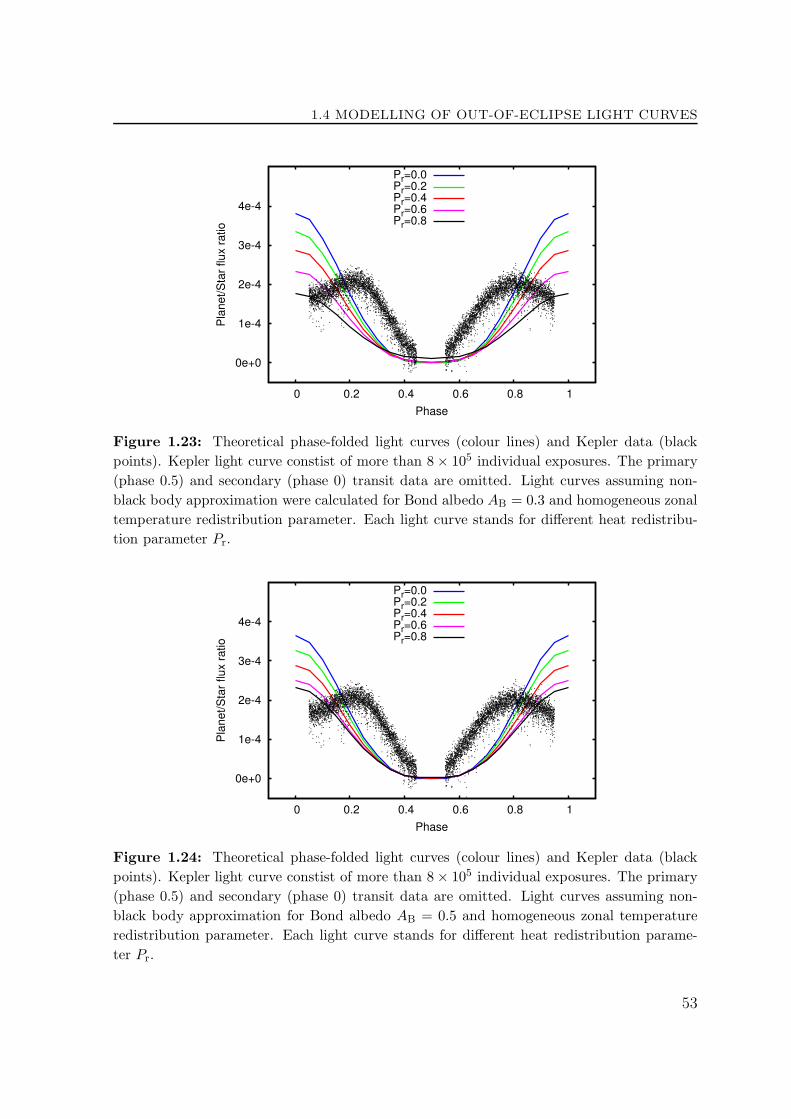
1.4 MODELLING OF OUT-OF-ECLIPSE LIGHT CURVES
0e+0
1e-4
2e-4
3e-4
4e-4
0 0.2 0.4 0.6 0.8 1
Pla
net/S
tar
flux r
atio
Phase
Pr=0.0Pr=0.2Pr=0.4Pr=0.6Pr=0.8
Figure 1.23: Theoretical phase-folded light curves (colour lines) and Kepler data (black
points). Kepler light curve constist of more than 8× 10⁵ individual exposures. The primary
(phase 0.5) and secondary (phase 0) transit data are omitted. Light curves assuming non-
black body approximation were calculated for Bond albedo AB = 0.3 and homogeneous zonal
temperature redistribution parameter. Each light curve stands for different heat redistribu-
tion parameter Pr.
0e+0
1e-4
2e-4
3e-4
4e-4
0 0.2 0.4 0.6 0.8 1
Pla
net/S
tar
flux r
atio
Phase
Pr=0.0Pr=0.2Pr=0.4Pr=0.6Pr=0.8
Figure 1.24: Theoretical phase-folded light curves (colour lines) and Kepler data (black
points). Kepler light curve constist of more than 8× 10⁵ individual exposures. The primary
(phase 0.5) and secondary (phase 0) transit data are omitted. Light curves assuming non-
black body approximation for Bond albedo AB = 0.5 and homogeneous zonal temperature
redistribution parameter. Each light curve stands for different heat redistribution parame-
ter Pr.
53

CHAPTER 1. LIGHT CURVES OF TRANSITING EXTRASOLAR PLANETS
0e+0
1e-4
2e-4
3e-4
4e-4
0 0.2 0.4 0.6 0.8 1
Pla
net/S
tar
flux r
atio
Phase
Pa=0.0Pa=0.2Pa=0.4Pa=0.6Pa=0.8Pa=1.0
Figure 1.25: Theoretical phase-folded light curves (colour lines) and Kepler data (black
points). Kepler light curve constist of more than 8× 10⁵ individual exposures. The primary
(phase 0.5) and secondary (phase 0) transit data are omitted. Light curves assuming non-
black body approximation for Bond albedo AB = 0.0 and heat redistribution parameter
Pr = 0.8. Each light curve stands for different value of degree of the inhomogeneity of the
heat transport Pa.
0e+0
1e-4
2e-4
3e-4
4e-4
0 0.2 0.4 0.6 0.8 1
Pla
net/S
tar
flux r
atio
Phase
Pa=0.0Pa=0.2Pa=0.4Pa=0.6Pa=0.8Pa=1.0
Figure 1.26: Theoretical phase-folded light curves (colour lines) and Kepler data (black
points). Kepler light curve constist of more than 8× 10⁵ individual exposures. The primary
(phase 0.5) and secondary (phase 0) transit data are omitted. Light curves assuming non-
black body approximation for Bond albedo AB = 0.5 and heat redistribution parameter
Pr = 0.0. Each light curve stands for different value of degree of the inhomogeneity of the
heat transport Pa.
54

1.4 MODELLING OF OUT-OF-ECLIPSE LIGHT CURVES
0e+0
1e-4
2e-4
3e-4
4e-4
0 0.2 0.4 0.6 0.8 1
Pla
net/S
tar
flux r
atio
Phase
Pa=0.0Pa=0.2Pa=0.4Pa=0.6Pa=0.8Pa=1.0
Figure 1.27: Theoretical phase-folded light curves (colour lines) and Kepler data (black
points). Kepler light curve constist of more than 8× 10⁵ individual exposures. The primary
(phase 0.5) and secondary (phase 0) transit data are omitted. Light curves assuming non-
black body approximation for Bond albedo AB = 0.0 and heat redistribution parameter
Pr = 0.6. Each light curve stands for different value of degree of the inhomogeneity of the
heat transport Pa.
we concentrated on the modelling of the reflected and thermal component, which are
the most pronounced effects in the light curve (we did not take into account ellipsoidal
variations and boosting effect). Consequently, our interpretation of results is based on
the areas of the light curve in the vicinity of transit and occultation (phases 0.5 and 0).
The effects of ellipsoidal variations and boosting are most pronounced at the phases
0.25 and 0.75.
The plots 1.20–1.27 indicate that the light curve (composed of Kepler data points)
better correspond to the models with rather low values of the Bond albedo AB and
higher values of the heat redistribution parameter Pr. We estimated the value of
Bond albedo to be AB < 0.3 and the value of the heat redistribution parameter to
be Pr > 0.6. The zonal temperature redistribution parameter Pa does not seem to
influence the shape of the light curve significantly (Figures 1.25–1.27). This analysis
shows that the atmosphere of extrasolar planet KOI-13.01 should be non-reflective and
dark, and that the process of heat transfer is rather significant for this planet.
Our results correspond with the previously published studies about exoplanetary
albedos. Cowan & Agol (2011) statistically studied albedos of 24 transiting exoplanets
and concluded that all these exoplanets are consistent with the low value of Bond
albedo. Mazeh et al. (2012) derived the Bond albedo and geometrical albedo of KOI-
13.01 as a function of the day-side planetary temperature. The value of the Bond
55

CHAPTER 1. LIGHT CURVES OF TRANSITING EXTRASOLAR PLANETS
albedo is supposed to be rather low (< 0.4) for a day-side temperature higher than
3400K.
Results described in this section were presented in the form of a poster at the Sagan
Exoplanet Summer Workshop held in Pasadena in the USA in 2012.
56

Chapter 2Star{planet intera tion2.1 Introduction
Planetary and stellar system bodies (stars, planets, their satellites) are not isolated
objects. They could influence or interact with one another in many possible ways. The
way of the interaction is usually quite complex. We know many such examples from
our own solar system. One that is worth mentioning is the Jupiter–Io system (de Pater
& Lissauer, 2001). As a result of Io’s close proximity to Jupiter, it is constantly heated
by tidal forces from Jupiter, which leads to melting of Io’s interior. Another effect is
the interaction of Io with Jupiter’s magnetosphere. The rotation period of Jupiter is
less than 10 hours and the orbital period of Io is 1.77 days. As Io moves through the
magnetosphere, which tend to corotate with Jupiter, an electric potential difference
between Io and Jupiter arises. The potential difference causes a current of nearly 106A
to flow along the magnetic field lines between Jupiter and Io. On the other hand, most
of the charged particles trapped in Jupiter’s magnetic field came from Io.
One of the major groups of extrasolar planets discovered so far is (as mentioned in
Introduction) Hot Jupiters. These Jupiter-sized planets orbit their parent stars at very
close distance. Consequently a vast number of interesting effects could occur between
them. Evaporation of the planet (Vidal-Madjar et al., 2003; Hubbard et al., 2007);
precession of the periastron due to general relativity (Jordan & Bakos, 2008), strong
irradiation of the planet and its effect on the planetary radius (Guillot & Showman,
2002; Burrows et al., 2007) or atmospheric and stratospheric processes (Hubeny et al.,
2003; Burrows et al., 2008; Fortney et al., 2008) are only a few examples from the long
list.
One of the most interesting effects which are expected to occur between the star
and exoplanet are the tidal and magnetic interaction. Cuntz et al. (2000) made a first
attempt to estimate the magnitude of such a possible tidal and magnetic interactions.
They calculated the relative strength of the star–planet interactions for 12 selected exo-
planetary systems with the distance of d . 0.1AU. Most of the host stars in the sample
57

CHAPTER 2. STAR–PLANET INTERACTION
were solar-type stars, which were supposed to have chromospheres, transition regions
and coronae. In case the planet somehow influences the star, it would affect mainly
the upper layers of the stellar atmosphere, because of its low density and proximity to
the planet.
The tides raised on the star affect the convective zone, as well as the outer layers
of the star. In the case the Prot 6= Porb (systems are not rotationally synchronized)
the tidal bulge rises and drops down to cause the expansion and contraction of the
outer layers. This process causes the flows and waves, which result in a significantly
higher production of nonradiative energy. This will lead to enhanced heating and a
higher level of stellar activity. Magnetic interaction is supposed to occur between stellar
active regions and the extrasolar planet magnetosphere. The magnetosphere of Hot
Jupiters is expected to strongly resemble that of the Jovian one in the work of Cuntz
et al. (2000). They found, that the strength of tidal and magnetic interaction depends
among others on the separation of the objects, size of the planet and magnetic field
strength of the star and planet.
This problem is similar to processes occuring in the RS Canum Venaticorum (here-
after RS CVn) systems (Hall, 1976). RS CVn are chromospherically active detached
binaries with periods of approximately 0.5 to 14 days (for some types the period can
reach 140 days). These systems consist of a slightly evolved stars of spectral type F,
G or early K and of luminosity class II–V. They are active as a result of the relatively
rapid rotation of at least one component. The majority of the RS CVn binaries have
the rotation of their active components synchronized with their orbital motion (Schri-
jver & Zwaan, 2000). The enhanced activity caused by this interaction is manifested
by starspots, chromospheric and coronal activity, and flares. As a consequence of the
presence of unevenly distributed starspots (these could cover a significant part of the
stellar surface) across the surface, the system shows photometric variability. In RS
CVn systems, the observed levels of chromospheric and coronal activity are higher
than for single stars of the same spectral class.
Rubenstein & Schaefer (2000) suggested that the superflares observed on nine F–G
main-sequence stars, which is an effect very similar to the one detected in RS CVn
systems, can be caused by the close proximity of an exoplanet and its consequent
interaction.
This chapter is focused on the search for star–planet interaction in exoplanetary
systems. Our goal of this work was to investigate the possible correlation between the
stellar activity and the orbital and physical parameters of the orbiting exoplanet.
58

2.1 INTRODUCTION
Figure 2.1: The core of the Ca IIK line in the spectrum of the Sun. Taken from Shkolnik
(2004).
2.1.1 Ca IIH and K lines
The most suitable regions of the spectra for observing chromospheric and coronal ac-
tivity are UV, EUV and X-rays. These were observed from space by, e.g. the IUE,
ROSAT, and XMM-Newton missions. However, the chromospheric activity can be also
observed in the optical region from the ground in the cores of several spectral lines:
the H and K lines of singly ionized calcium (3933, 3968 A), the D lines of neutral
sodium (5889, 5895 A), He I D3 (5876 A) and Hα (6563 A). Of these, Ca IIH and K
lines were of special interest. These lines are very strong and their core is formed in the
chromosphere of the star, hence were used for surveys of stellar chromospheric activity,
see Hall (2008) and references therein.
Figure 2.1 shows the structure of the Ca IIK line of the Sun. K1 point marks the
turn over part of the absorption feature when it changes into the emission. It is formed
at the top of the photosphere. The feature denoted as K2 is a double-peaked emission
that is formed in the chromosphere at temperature of about 8 000K. The self-reversal
core (due to the large optical depth of the line) is marked as K3 and is produced at the
top of the chromosphere where the temperature reaches 20 000K. Figure 2.2 shows the
atmospheric model of the Sun and the depths were different spectral lines are formed,
the origin of Ca IIH and K lines included.
The presence of the emission components in the cores of the Ca IIH and K resonance
lines in the spectra of many stars of spectral type G and later has been a known fact
for a long time. Eberhard & Schwarzschild (1913) found out that the stellar K and H
59

CHAPTER 2. STAR–PLANET INTERACTION
Figure 2.2: The average quiet-Sun temperature distribution. The approximate depths where
the various continua and lines originate are indicated. The plot is adopted from Vernazza
et al. (1981).
lines of calcium show a sharp reversal, with the calcium emission in the middle of the
absorption line just as it is observed in the Sun.
2.1.2 Mt.Wilson observations
The Ca IIH and K lines were chosen by O.C.Wilson for a long-term, ground-based
survey of stellar activity in order to reveal the analog of the Sun’s 11 year activity
cycle in other stars (Wilson, 1968, 1978). This systematic research, which took place
on Mount Wilson Observatory began in 1966 and continued for more than 40 years.
The original instrument used for the observations was the photoelectric coude scanner
at the 100 inch telescope. In 1977 it was replaced by a four channel (R, V,H,K)
spectrophotometer (Vaughan et al., 1978) The photoelectric coude scanner was then
removed from the 100 inch telescope and moved to the 60 inch telescope.
Amongst the most important results of this survey, summarized in Duncan et al.
(1991) and Baliunas et al. (1995), was the discovery of activity cycles in solar-type
stars, similar to those of the Sun. In addition a number of stars showed evidence of
uncompleted cycles of duration greater than 11 years, and many showed real variability
at time scales from one day to several months.
60

2.2 SEARCH FOR STAR–PLANET INTERACTION
The survey contributed towards an understanding of the evolution of stellar activity
and stellar rotation. With the Mt.Wilson project it was proved that chromospheric
activity of main-sequence stars decreases with age and that their rotational periods
can be determined from the rotational modulation of Ca IIH and K emission (Vaughan
et al., 1981).
For a quantitative description of the Ca IIH and K line flux, an instrumental S index
was introduced (Middelkoop, 1982):
S ≡ αNH +NK
NR +NV, (2.1)
where α = 2.4 is the constant of proportionality, NH, NK, NR, and NV are the num-
ber of counts in the corresponding channels. R (3991.07–4011.07 A) and V (3891.07–
3911.07 A) channels are 20 A-wide continuum bands. Triangular shaped channels H
and K are centered on the cores of the Ca IIH and K lines.
S index has a disadvantage that it cannot be used to compare stars of different
spectral types. It includes both the chromospheric emission and the flux from the
photosphere. As the continuum flux decreases through the spectral type sequence, the
S index tends to increase. A new parameter – logR′
HK –was introduced in order to
remove the photospheric component from the S index and to determine the fraction of
a star’s luminosity that is in the Ca II H and K lines (Middelkoop, 1982; Noyes et al.,
1984; Wright et al., 2004). The R′
HK parameter is calculated as:
R′
HK = RHK − Rphot, (2.2)
where
RHK = 1.340× 10⁻⁴CefS. (2.3)
The colour-dependent conversion factor Cef(B − V ) is:
logCef(B − V ) = 1.13(B − V )3 − 3.91(B − V )2 + 2.84(B − V )− 0.47, (2.4)
where the Rphot is a photospheric component. This relation was derived only for main-
sequence stars with 0.45 ≤ (B − V ) ≤ 1.50. The Rphot parameter is then calculated
as:
logRphot = −4.898 + 1.918(B − V )2 − 2.893(B − V )3. (2.5)
The resulting parameter logR′
HK increases with higher activity.
2.2 Search for star–planet interaction
As stated in previous sections, the idea of possible influence of the stars by orbiting
objects (planets, stars) is not new. In the last decade, the extensive searches for star–
planet interaction in the whole energy spectrum from the ground as well as from space
61

CHAPTER 2. STAR–PLANET INTERACTION
were carried out. In this section I give only brief review about this phenomenon,
mentioning the most important results.
Shkolnik et al. (2003, 2005, 2008) presented a set of papers concerning the search for
modulation (variation) of selected lines in the spectra of stars with close-in exoplanets
in phase with the planetary orbit. They observed selected stars with exoplanets with
the 3.6m Canada-France-Hawai Telescope in the optical region. Their observing runs
span over several years and they monitor the activity preferentially in the cores of
Ca IIH and K lines. As a result they found an evidence for variations in Ca II emission
connected with the orbital period of close-in exoplanet.
Knutson et al. (2010) studied the correlation between the activity of the host star
and the type of the atmosphere of exoplanet. For a sample of 50 transiting exoplanets
they measured the strength of the Ca IIH and K lines and consequently determined
the logR′
HK parameter (defined by Equation 2.2). They found that planets orbiting
chromospherically active stars have so-called “non-inverted” atmospheres (HD189733,
Tres-1, Tres-3, and Wasp-4), while atmospheres of planets orbiting quiet stars show a
strong high-altitude temperature inversion (e.g. HD209458, Tres-2, Tres-4, Hat-p-7,
and Wasp-1). This finding was explained as that the more active stars emit more in
the UV region and this radiation destroys the high-altitude absorber responsible for
the formation of temperature inversions.
Based on the data from Knutson et al. (2010), Hartman (2010) searched for a cor-
relation between stellar activity (described by the logR′
HK parameter) and 12 different
exoplanetary parameters. They found a correlation between the planet surface gravity
log gp and the logR′
HK parameter with greater than 99.5% confidence. However the
nature of this correlation was not sufficiently clarified.
Gonzalez (2011) claims that stars with exoplanets have lower values of parameters
v sin i and logR′
HK (i.e. less activity) than stars without exoplanets.
Kashyap et al. (2008) searched for X-ray activity in more than 200 planet-hosting
stars. They found a statisticaly significant evidence that stars with close-in planets are
more active than the stars with exoplanets located further out.
The complex study of star–planet interaction in the X-ray region was made by Pop-
penhaeger et al. (2010). They studied the stellar X-ray activity of all known exoplanet
host stars within a distance of 30 pc. Their sample consisted of 72 exoplanetary systems
and they used the quantity Lx/Lbol as an activity indicator. Lx is the X-ray luminosity
of the star and Lbol is its bolometric luminosity. They did not find any correlation
between the coronal activity of the star and the planetary parameters semi-major axis
a, mass of the planet Mp, and Mp/a. The dependencies observed in the sample were
dismissed by the authors as statistical fluctuations or selection effects.
62

2.2 SEARCH FOR STAR–PLANET INTERACTION
5000 5500 6000 6500Stellar T
eff (K)
-5.6
-5.4
-5.2
-5.0
-4.8
-4.6
-4.4
-4.2
Log(
Rl H
K)
TrES-1
HD 189733TrES-3
WASP-4
CoRoT-2
WASP-2XO-2 XO-1
TrES-2HAT-P-1HD 209458
XO-3
HAT-P-7TrES-4
WASP-1
CoRoT-1
WASP-18
K0 G8 G5 G2 G0 F8
Figure 2.3: Dependence of the logR′
HK parameter on stellar effective temperature. Exo-
planets with temperature inversion orbiting less active stars are marked with circles. The
star symbols are for exoplanets without temperature inversion. The grey area on the right
side of the plot marks the region for which is the logR′
HK parameter is not defined. Taken
from Knutson et al. (2010).
Scharf (2010) studied the X-ray emission of stars hosting planets. He found a
positive correlation between the X-ray luminosity of the parent stars and the Mp sin i
parameter of most close-in exoplanets with periastron distance dperi < 0.15AU.
This interesting discovery motivated Poppenhaeger & Schmitt (2011) to re-analyse
the data from Scharf (2010). They focused on possible selection effects which could
occur in the selected sample. To make the sample of data robust enough, they included
data from previous studies (Poppenhaeger et al., 2010) as well. They found that the
dependence presented in Scharf (2010) is a consequence of selection effects caused by
the flux limit of the data sample used in Scharf (2010) and also by planet detectability
by the RV method.
Canto Martins et al. (2011) analysed a sample composed of stars with and without
extrasolar planets. They searched for a dependence of the chromospheric and the X-ray
emission flux on the planetary parameters log(1/aP) and log(MP/aP) (where aP is a
semi-major axis and MP is a planetary mass). As a chromospheric and coronal activity
indicator they used parameters logR′
HK and (logLx/Lbol), respectively. Their sample
consisted of 74 stars with exoplanets (detected by radial velocity method) and of 26
stars without extrasolar planets. Their statistical analysis did not reveal any convincing
proof for the correlation between the chromospheric activity and the aforementioned
planetary parameters.
63

CHAPTER 2. STAR–PLANET INTERACTION
Alves et al. (2010) investigated the projected rotational velocity, v sin i, and stellar
angular momentum of 147 stars with extrasolar planets and 85 stars with no compan-
ions. Exoplanetary systems covered in the sample were detected by the RV technique
only. The most interesting result of their work was that the angular momentum of
stars without exoplanets shows a clear deficit when compared to stars with planets.
This effect is most pronounced for stars with mass higher than 1.25M⊙.
2.3 Spectroscopic observations and data
In this Section the observing strategies and reduction process of data used for the
subsequent statistical analysis are described.
Stellar spectra used in our study originate from two different sources. The main
source is the publicly available Keck HIRES spectrograph archive and the sample con-
sists of 206 stars with exoplanets. These data were enhanced by our own observations
of four stars (HD179949, HD212301, HD149143 and Wasp-18) with a close-in exo-
planet. We obtained these data with the FEROS spectrograph mounted on the 2.2m
ESO/MPG telescope in Chile. In all of the following plots, the data from 2.2m tele-
scope are marked as red squares.
The sample of data contains 210 exoplanet hosting stars with an effective temper-
ature range of approximately 4 500 to 6 600K. The semi-major axes of the exoplanets
lie in the interval 0.016–5.15AU.
2.3.1 2.2m MPG/ESO telescope –Observations and data re-
duction
FEROS is a fibre-fed echelle spectrograph with a resolution of up to 48 000 and with
a spectral coverage from 350 to 920 nm. It is mounted at the Cassegrain focus of the
2.2m MPG/ESO telescope at La Silla observatory in Chile. A thorium-argon-neon
lamp is used for wavelength calibration.
For the purpose of studying star–planet interaction, we observed four exoplanetary
systems HD179949, HD212301, HD149143, and Wasp-18 with the FEROS instrument.
We selected these systems from the list of discovered exoplanets according to the ex-
pected amplitude of variability parameter Mp sin i/Porb multiplied by an expected S/N.
We ruled out the exoplanets with orbital periods larger than was the duration of the
observing run. The spectra of the objects together with the calibration frames (bias,
flat, and calibration frames) were taken during five and half consecutive nights. For
the consequent statistical analysis described in Section 2.4 only data from the night
with the best observing conditions (18/19.9.2010) were used.
64

2.3 SPECTROSCOPIC OBSERVATIONS AND DATA
Reduction process
The echelle spectra were reduced following the standard procedures. Packages suitable
for echelle spectra implemented in IRAF1 were used.
For the combination of biases the package ccdred, task zerocombine was used
and an average frame was created. Minmax rejection was used, whereby a fraction
of the highest and lowest pixels were rejected to omit over exposed pixels. After
that the bias was subtracted from flats, comps and objects using package imutil,
task imarith. This task is performing basic operations with frames, like addition,
subtraction, multiplication, etc. The corrected flats were combined into one master flat
with package ccdred, task flatcombine. In the next step we removed the large scale
variability seen in the master flat using the task apflatten in the package echelle,
leaving only pixel-to-pixel variation. This task finds the individual orders, fits the
selected function to the intensity along the dispersion and normalizes the flat field
with the fit. To avoid a possible zero signal between the orders (numerical reasons),
this task replaces the points with a low signal with the integer stated for the treshold
parameter.
Object frames were divided by the resulting master flat using the package imutil,
task imarith. After that a mask for bad pixels was created using package proto, task
fixpix. Bad pixels were found manualy in one flatfield frame and the resulting mask
was applied to all the object frames.
The next step was the extraction of the apertures from the 2-dimensional spectra.
This was done by the summation of pixels across the dispersion axis. Package echelle,
task apsum was used. This task was also applied to the wavelength calibration frames.
The extracted spectra need to be calibrated for the wavelength. For this the calibration
frames of the ThArNe lamps were taken. These are spectra with precisely defined and
calibrated emission features. By comparing them to the spectra of an object, it is
possible to assign accurate wavelength values to the spectra of the object. As a first
step, the identification of the spectral lines in the calibration frame must be done. For
this, the package echelle, task ecidentify was used, where the database of emission
spectral lines for the employed lamp was used. After that, the spectra with identified
lines are applied to the object frames and the spectra are wavelength calibrated.
The continuum of the spectra of the object need to be normalized, for which the
package echelle, task continuum was used. This task fitts the continuum with a
spline function of specified order and then the spectrum is divided by it.
One of the last steps is the combination of individual spectra of each object into
a single spectrum. This was done by the package onedspec, task scombine. Finally
1http://iraf.noao.edu/
65

CHAPTER 2. STAR–PLANET INTERACTION
5000
10000
15000
20000
3930 3931 3932 3933 3934 3935 3936 3937 3938 3939
Rela
tive F
lux
Wavelength [A]
HD 189733HD 7924
Figure 2.4: Illustration of the core of the Ca IIK line in two different stars. We measured
only the equivalent width of the core of the line with the central reversal. By definition,
equivalent width is negative for emission and positive for absorption.
heliocentric correction was calculated (package rv, task rvcorrect) and applied to the
spectra (package echelle, task dopcor).
2.3.2 Keck HIRES archive data
The main part of the data used in the statistical study comes from the HIRES instru-
ment mounted on the Keck I telescope.1 HIRES stands for High Resolution Echelle
Spectrometer with a resolution of up to 85 000. The instrument is mounted at the
Nasmyth focus and its range spans from 0.3 to 1.1µm (Vogt et al., 1994).
For our analysis, we used data from the archive of the HIRES instrument.2 From the
archive we carefully selected only those spectra with a signal-to-noise ratio high enough
to measure the precise equivalent width (hereafter EQW) of the Ca IIK emission. The
data in the archive were reduced by an automated reduction pipeline based upon the
HIRES data reduction package MAKEE.3
1This research has made use of the Keck Observatory Archive (KOA), which is operated by the
W.M.Keck Observatory and the NASA Exoplanet Science Institute (NExScI), under contract with
the National Aeronautics and Space Administration.2http://www2.keck.hawaii.edu/koa/public/koa.php3http://www.astro.caltech.edu/~tb/makee/index.html
66

2.4 STATISTICAL ANALYSIS OF THE DATA SAMPLE
2.3.3 Equivalent width measurements
For each spectrum in the sample, we measured the EQW (in A) of the central reversal
in the core of lines Ca IIK and Ca IIH. The IRAF software was used for this purpose,
namely the package onedspec, task splot. Figure 2.4 illustrates a placement of the
pseudo-continuum in our measurements. The advantage of using such a simple EQW
measurement is that this is defined on a short spectral interval that is about one A wide.
Consequently, it is not sensitive to the various calibrations (continuum rectification,
blaze function removal) inherent in echelle spectroscopy. For comparison, the logR′
HK
index relies on the information from four spectral channels covering about a 100 A wide
interval. If extracted from echelle spectra, it is much more sensitive to a proper flux
calibration and subject to added uncertainties.
Originally, we measured the EQW of the cores of both Ca IIK and Ca IIH lines.
For the analysis, we decided to use the EQW of Ca IIK only, because the Ca IIH line
is strongly blended by the Hǫ Balmer line. Nevertheless, as a check, we plotted two
dependencies: Teff vs. EQWCa II H in Figure 2.12 and semi-major axis vs. EQWCa IIH
in Figure 2.13.
For comparison with our EQW values, we also used the parameter logR′
HK defined
in Equation (2.2). Values of this parameter were taken from the works of Wright et al.
(2004), Knutson et al. (2010), and Isaacson & Fischer (2010).
The list of all the exoplanets, their properties, and measured equivalent width
together with the logR′
HK parameter used in this study, are in Appendix D.
2.4 Statistical analysis of the data sample
Most of the previous studies focused on either the monitoring of stellar activity of an
individual star connected with the orbital period of an exoplanet, or on comparing two
samples of stars, mostly with and without exoplanets. The main goal of this section
was to search for a possible correlation between exoplanetary orbital and physical
parameters and stellar activity in the sample of stars with exoplanets.
In Figure 2.5 (top part) the EQW of Ca IIK emission core versus the effective
temperature Teff of the star is depicted. By definition, the EQW is negative for emission.
Consequently, lower values mean higher emission and higher chromospheric activity.
The dependence of EQW on temperature is immediately apparent, mostly in the lower
temperature region. The EQW decreases in this region, which means that the core
emission increases towards lower temperatures. This feature is not surprising and is
partially a result of the fact, that the photospheric flux in the core of the Ca IIK line
is lower for cooler stars than for hotter stars. At the same time, the data points that
67

CHAPTER 2. STAR–PLANET INTERACTION
0
0.2
0.4
0.6
0.8
1
4500 5000 5500 6000 6500
Sig
nific
ance
Teff [K]
T testK-S test
-5.0
-4.0
-3.0
-2.0
-1.0
0.0
1.0
EQ
WC
a II K [A
]
a ≤ 0.15 AUa > 0.15 AU
FEROS a < 0.15 AU
Figure 2.5: Top: dependence of the equivalent width of the Ca IIK emission on the temper-
ature of the parent star. Triangles denote data from HIRES, red squares denote data from
FEROS. Exoplanetary systems with a ≤ 0.15AU are marked with empty triangles, systems
with a > 0.15AU are marked with full triangles. FEROS sample consists of exoplanets with
semi-major axis a < 0.15AU only. Bottom: results of statistical Student’s t-test (empty
circles) and Kolmogorov–Smirnov test (full circles) for each of the temperature window as
described in the text.
symbolize stars with Teff > 5 500K show only a narrow spread of Ca IIK EQWs, while
cooler stars have a broad range of these values.
In the first step, we aimed to study the possible connections between the semi-
major axes of extrasolar planets and the EQW of Ca IIK line core. In the top part of
Figure 2.5 we distinguished between stars with close-in and far-out exoplanets. Stars
harboring planets with semi-major axes shorter than 0.15AU are marked with upside
down white triangles, while the rest, with semi-major axes longer than 0.15AU, are
marked with black triangles. We divided the sample in this way for two reasons. The
first one was the visual inspection of Figure 2.9. A second reason for this division is
the theoretical assumption that most exoplanets orbiting solar-type stars with orbital
distance less than 0.15AU are presumed to rotate synchronously with their orbital
period (Bodenheimer et al., 2001). The fact that stars with close-in planets tend to
have higher Ca IIK emission (lower EQWs) than stars with distant planets, can be
68

2.4 STATISTICAL ANALYSIS OF THE DATA SAMPLE
0
0.2
0.4
0.6
0.8
1
4500 5000 5500 6000 6500
Sig
nific
ance
Teff [K]
T testK-S test
-5.0
-4.0
-3.0
-2.0
-1.0
0.0
1.0
EQ
WC
a II K [A
]
a ≤ 0.15 AUa > 0.15 AU
FEROS a < 0.15 AU
Figure 2.6: Top: dependence of the equivalent width of the Ca IIK emission on the temper-
ature of the parent star for systems discovered by the RV method only. Triangles denote data
from HIRES, red squares denote data from FEROS. Exoplanetary systems with a ≤ 0.15AU
are marked with empty triangles, systems with a > 0.15AU are marked with full triangles.
FEROS sample consists of exoplanets with semi-major axis a < 0.15AU only. Bottom: re-
sults of statistical Student’s t-test (empty circles) and Kolmogorov–Smirnov test (full circles)
for each of the temperature window as described in the text.
69

CHAPTER 2. STAR–PLANET INTERACTION
0
0.2
0.4
0.6
0.8
1
4500 5000 5500 6000 6500
Sig
nific
ance
Teff [K]
T testK-S test
-6
-5.5
-5
-4.5
log R
’ HK
a ≤ 0.15 AUa > 0.15 AU
FEROS a < 0.15 AU
Figure 2.7: Top: dependence of the activity index logR′
HK on the temperature of the
parent star. Triangles denote data from HIRES, red squares denote data from FEROS.
Exoplanetary systems with a ≤ 0.15AU are marked with empty triangles, systems with
a > 0.15AU are marked with full triangles. FEROS sample consists of exoplanets with semi-
major axis a < 0.15AU only. Bottom: results of statistical Student’s t-test (empty circles)
and Kolmogorov–Smirnov test (full circles) for each of the temperature window as described
in the text.
70

2.4 STATISTICAL ANALYSIS OF THE DATA SAMPLE
readily seen in Figure 2.5. In Figure 2.9 a difference in activity scatter for close and
distant planets can be seen as well.
To verify whether this visual finding is statistically significant, we performed two
statistical tests on these two data samples. The first one was the Student’s t-test
(hereafter T test) and the second one was the Kolmogorov–Smirnov test (hereafter K–S
test) see Appendix C. We studied whether the sample of stars with close-in exoplanets
differs in a statistically significant way from the sample of stars with distant planets.
In the case of Student’s t-test, the null hypothesis is the statement: Two data sets
have the same mean. Two means are significantly different if the Student’s distribution
probability density function A(t | ν) is higher than our pre-selected value. This value
is usually 0.95 or 0.99. Consequently the significance level at which the hypothesis
that the means are equal is disproved, is defined as: 1 − A(t | ν). The significance is
a number between 0 and 1. A small significance value (0.05 or 0.01) means that the
obtained difference is very significant.
For the K–S test is the null hypothesis the statement: Two data sets are drawn
from the same population distribution function.
Instead of studying both samples directly, we selected a running window that was
400K wide and that ran along the temperature axis in steps of 50K. Only a definite
number of data points from each sample fell inside each window. The statistical tests
mentioned above were performed on these restricted data samples. The bottom panel
of Figure 2.5 shows the resulting values of significance level, labeled as significance
in all the plots for each test, and these are plotted versus the center of the current
temperature window. The results of the tests (as a function of temperature) show
whether the two samples have the same mean or originate from the same distribution
function. Figure 2.5 shows that in the region of smaller temperatures (Teff ≤ 5 500K)
the significance is less than 0.05 for both the K–S and T test respectively. The null
hypotheses can be disproved on the selected level of significance for the stars with
the temperature smaller than 5 500K. Consequently the difference between the stars
with close-in and distant exoplanets is statistically significant for cooler stars with
Teff ≤ 5 500K. On the other hand, the statistical test applied to the hot stars did not
show any statistical significance to indicate that the two samples are different.
Before interpreting these results, the selection effects in the sample need to be
taken into account. To investigate the impact of selection effects on our results, we
omitted the stars with transiting exoplanets from our sample. In Figure 2.6 we plotted
the temperature–EQW dependence for this restricted data set. On this reduced data
sample, we performed the same statistical tests as for the complete sample, by choosing
the same temperature binning for the running window. The results are plotted in the
bottom panel of Figure 2.6. Even if the transit data are excluded, the tests show a
significant difference between the stars with close-in and distant exoplanets for the
71

CHAPTER 2. STAR–PLANET INTERACTION
cold stars. However, the size of the sample (especially the number of exoplanets on
close-in orbits) has substantially decreased, which made the results of statistical tests
less trustworthy.
To verify these trends, we also explored the dependence of the logR′
HK parameter
on the effective temperature of the star (Figure 2.7). This parameter does not show
a strong temperature dependence and was described in more detail in Section 2.1.2.
Two samples, distinguished by triangle marks according to the semi-major axis of the
orbiting exoplanet, can be seen in the top panel of the figure. It is apparent that stars
with close-in planets show a wider range of logR′
HK values than the stars with more
distant planets. Cooler stars (Teff ≤ 5 500K) with close-in planets have higher values
of logR′
HK and thus higher chromospheric activity.
We performed the same statistical test with the same procedure as described in the
paragraphs above. The result is plotted in the bottom part of Figure 2.7. The vertical
axis in this figure (and in all the following figures with logR′
HK parameter dependence)
is in the reverse order. The higher value of logR′
HK parameter, the higher is the
stellar activity. The motivation was to unify the direction of increasing stellar activity
with the EQW dependencies. The statistical test yielded almost the same result as
in the previous cases. The difference between stars with close-in and distant planets
is statistically significant for Teff ≤ 5 500K. The values of the significance resulting
from both statistical tests lie mostly under the 0.05 value and the hypotheses, that the
two samples come from one distribution function and have the same mean could be
disproved at the 0.05 significance level.
Figure 2.8 depicts the temperature–logR′
HK dependency for the stars with exoplan-
ets discovered by the RV technique only. The same tests as in the previous cases were
applied and the resulting significance value is smaller than 0.05 for the cooler stars.
Semi-major axis dependence
In the preceding section we found statistically significant evidence that the chromo-
spheric activity of the cold stars is connected with the semi-major axis of the orbiting
exoplanet. We thus continue exploring the possibility of such a connection in this
section. Figure 2.9 gives a plot of the dependence of the EQW of the Ca IIK emis-
sion on the semi-major axis. Following the results of the statistical tests depicted in
Figures 2.5–2.8, we selected only systems with Teff ≤ 5 500K. Two distinctive pop-
ulations are clearly visible in the plot in Figure 2.9. Stars with close-in exoplanets
(a ≤ 0.15AU) have a broad range of the Ca IIK emission, while stars with distant
planets (a > 0.15AU) have a narrow range of weak Ca IIK emission. As before a
distinction is made in the plot between stars with planets discovered by the RV and
transit methods. Apparently a significant fraction of stars with close-in exoplanets
(but not all of them) have a high Ca IIK emission. However, this result may again be
72

2.4 STATISTICAL ANALYSIS OF THE DATA SAMPLE
0
0.2
0.4
0.6
0.8
1
4500 5000 5500 6000 6500
Sig
nific
ance
Teff [K]
T testK-S test
-6
-5.5
-5
-4.5
log R
’ HK
a ≤ 0.15 AUa > 0.15 AU
FEROS a < 0.15 AU
Figure 2.8: Top: dependence of the activity index logR′
HK on the temperature of the parent
star for systems discovered by the RV method only. Triangles denote data from HIRES, red
squares denote data from FEROS. Exoplanetary systems with a ≤ 0.15AU are marked with
empty triangles, systems with a > 0.15AU are marked with full triangles. FEROS sample
consists of exoplanets with semi-major axis a < 0.15AU only. Bottom: results of statistical
Student’s t-test (empty circles) and Kolmogorov–Smirnov test (full circles) for each of the
temperature window as described in the text.
73

CHAPTER 2. STAR–PLANET INTERACTION
-6
-5
-4
-3
-2
-1
0
1
0.1 1 10
EQ
WC
a II K [A
]
a [AU]
RV dataTransit data
Figure 2.9: Dependence of the EQW of Ca IIK emission on the semi-major axis. Included
are only systems with Teff ≤ 5 500 K. Empty triangles are exoplanetary systems discovered
by the RV technique, full triangles are systems discovered by the transit method. Note that
the semi-major axis is logarithmic.
-5.5
-5
-4.5
-4
0.01 0.1 1 10
log R
’ HK
a [AU]
RV:T ≤ 5500 KRV:T > 5500 K
Trans:T ≤ 5500 KTrans:T > 5500 K
Figure 2.10: Dependence of the activity index logR′
HK on the semi-major axis. Triangles
are exoplanetary systems discovered by the RV technique, circles are systems discovered by
the transit method. Note that the semi-major axis is logarithmic.
74

2.4 STATISTICAL ANALYSIS OF THE DATA SAMPLE
-2
-1.5
-1
-0.5
0
0.5
1
1.5
2
0.01 0.1 1 10 100
EQ
W -
bT
eff -
d
MP sin i [MJ]
RV dataTransit data
Figure 2.11: Dependence of the modified equivalent width of the Ca IIK emission on planet
mass. Only stars with Teff ≤ 5 500K and a ≤ 0.15AU are considered. Empty triangles denote
stars with planets detected by the RV method, full triangles the transit method.
affected by selection biases. (It is more difficult to detect distant planets around active
stars.)
We also explored the logR′
HK parameter as a function of the semi-major axis. This
is illustrated in Figure 2.10, where is plotted the whole sample of exoplanetary systems
without any restrictions. As in the previous case, this figure shows a clear distinction
between the stars with close-in planets with semi-major axis less than 0.15AU and
the stars with distant planets. This is mainly caused by hotter stars with transiting
exoplanets. Should we concentrate on cold stars with exoplanets detected by the RV
technique only, there might be a trend for stars with close-in planets to have higher
logR′
HK values than stars with distant planets, but it is not as pronounced as in the
EQW measurements.
Mass dependence
The previous analysis result raises a question as to the reason for the high range of
the EQW of Ca IIK emission in the sample of cold stars with close-in planets. This
phenomenon can have a variety of explanations. It can be connected with the planet
orbital period, stellar activity cycle, or stellar ages. It can be a result of any other
process that affects the stellar chromosphere. We explored whether the scatter may
come from the eccentricity of the orbit, but we could not find any convincing evidence
for the eccentricity effect. If there is a dependence of the Ca IIK emission on the semi-
major axis of the planet, there ought to be some dependence on the mass of the planet,
75

CHAPTER 2. STAR–PLANET INTERACTION
Mp, as well. This dependence would have to be continuously reduced in the case of
sufficiently small planets. However only Mp sin i is known for most of the extrasolar
planets. Nevertheless we selected all stars with temperatures T ≤ 5 500K and with
semi-major axes a ≤ 0.15AU and fitted their EQWs of the Ca IIK emission using the
following function:
EQW (Mp, Teff) = bTeff + c log(Mp sin i) + d, (2.6)
where Mp is in the units of Jupiter mass. The usage of this function was motivated by
the intention to study the dependence of the mass of the planet on the EQW. However,
as was stated above, the EQW depends strongly on the temperature of the star. So
the EQW in the expression (2.6) is studied as a function of stellar temperature and
planetary mass. Within the fitting procedure we found the following coefficients:
b = 3.65× 10⁻³ ± 5.7× 10⁻⁴ [AK−1], (2.7)
c = −0.392± 0.097 [A], (2.8)
d = −20.4± 2.9 [A]. (2.9)
The b coefficient is significant beyond 6σ, so temperature dependence is very clear.
However, the c coefficient is also significant beyond 4σ, and it indicates the statistically
significant correlation of the chromospheric activity with the mass of the planet. We
applied a statistical F -test to justify the usage of an additional parameter (planet
mass) in the above mentioned fitting procedure. The null hypothesis was in this case
a statement: The model with 3 parameters does not give a significantly better fit
than the 2-parameter fit. The test shows that the significance of the 3-parameter fit
(Equation (2.6)) over the 2-parameter fit defined as:
EQW (Teff) = bTeff + d, (2.10)
is 0.003. This means that on the chosen level of significance of 0.05, the test disproved
the null hypothesis. These results are illustrated in Figure 2.11, where we plot the
modified equivalent width of the Ca IIK emission as a function ofmp sin i, showing stars
with planets detected by the RV and transit methods. The modified equivalent width
is EQW corrected for the strong temperature dependence, namely: EQW − bTeff − d.
Lower values of EQW mean higher emission, and thus the host stars with more massive
planets show more chromospheric activity. However this correlation might also be
affected by the selection effect that it is more difficult to detect a less massive planet
around a more active star.
76

2.4 STATISTICAL ANALYSIS OF THE DATA SAMPLE
-5
-4
-3
-2
-1
0
1
4500 5000 5500 6000 6500 7000
EQ
WC
a II H
[A
]
Teff [K]
a ≤ 0.15 AUa > 0.15 AU
FEROS a < 0.15 AU
Figure 2.12: Dependence of the equivalent width of Ca IIH emission on the temperature
of the star. Empty triangles are exoplanetary systems with a ≤ 0.15AU, full triangles are
systems with a > 0.15AU and red squares are our data from FEROS.
-4.5
-4
-3.5
-3
-2.5
-2
-1.5
-1
-0.5
0
0.5
1
0.01 0.1 1 10
EQ
WC
a II H
[A
]
a [AU]
RV dataTransit data
Figure 2.13: Dependence of the equivalent width of Ca IIH emission on the semi-major
axis. Empty triangles are exoplanetary systems discovered by RV technique, full triangles
are systems discovered by transit method.
77

CHAPTER 2. STAR–PLANET INTERACTION
2.5 Conclusion
In this chapter we focused on the study of possible interaction between the host star
and orbiting exoplanet. We searched for possible correlation between the stellar chro-
mospheric activity and the orbital and physical parameters of the exoplanet. As an
activity indicators were used two parameters – the equivalent width (EQW) of the core
of the Ca IIK line and logR′
HK index. Our sample of more than 200 exoplanetary
systems consists of data obtained with two different instruments. The major part of
the data were taken from the archive of intstrument HIRES, mounted on the Keck I
telescope. Data obtained with instrument FEROS located on La Silla in Chile form
the minor part of the sample.
Our main aim was the statistical study of the diversity of two subsamples of orig-
inal data, which were sorted out according to the semi-major axis a of the orbiting
exoplanet. First group consisted of stars with close-in exoplanets (semi-major axis less
than 0.15AU) and the second one consisted of systems with exoplanets located further
out (semi-major axis greater than 0.15AU).
For this purpose we performed two statistical tests – the Kolmogorov–Smirnov test
and Student’s t-test on our two data samples. As a result we found statistically sig-
nificant evidence that the EQW of the Ca IIK emission in the spectra of planet host
stars with effective temperature less than 5 500K as well as their logR′
HK activity in-
dex depend on the semi-major axis of the exoplanet (see Figures 2.5 and 2.7). More
specifically, cool stars (Teff ≤ 5 500K) with close-in planets (a ≤ 0.15AU) generally
have higher Ca IIK emission than stars with more distant planets. This means that
a close-in planet can affect the level of the chromospheric activity of its host star and
can heat the chromosphere of the star.
We also considered the selection effects caused by the discovery method of exoplan-
ets, since these can significantly distort the results. Our sample of more than 200 stars
consists of exoplanetary systems discovered by two different methods. These are the
RV method and the transit method (both these methods are described in the Intro-
duction together with the biases which are characteristic for each method). These two
techniques have very different criteria for selecting the exoplanetary candidates. The
RV measurements concentrate on low-activity stars, whereas transit technique does
not put any constraints concerning activity on the stars. In more detail, the general
sample of transiting exoplanets is biased towards the planets on close-in orbit. As a
consequence, the scatter among the data in the top part of Figure 2.5 (close-in exo-
planets orbiting cooler star) was caused mainly by a selection effect. Nevertheless, we
performed the same statistical test on the exoplanetary systems, divided according to
the semi-major axis and discovered by RV technique only. The results are given in the
78

2.5 CONCLUSION
Figures 2.6 and 2.8. The results of the statistical tests remained to be significant, even
for such a restricted sample.
Moreover, we have found statistically significant evidence that the Ca IIK emission
of the host star (for Teff ≤ 5 500K and a ≤ 0.15AU) increases with the mass of the
planet.
The biggest disadvantage of the analysis performed in this chapter is the size of the
RV exoplanets sample. The statistical tests depicted in Figures 2.6 and 2.8 are based on
quite a low number of exoplanets with semi-major axes smaller than 0.15AU. The need
for a larger data sample is evident in this case. Moreover the trends and correlation
may be affected by selection effects and should be revisited when less biased sample of
stars with planets becomes available.
Our results were presented in the paper Krejcova & Budaj (2012). Recently Shkol-
nik (2013) presented a study in the far ultraviolet (FUV) and near ultraviolet (NUV)
region of 272 stars hosting extrasolar planets. She concentrated on the search for
increased stellar activity caused by star–planet interaction. She found a statistically
significant evidence, that the stars with close-in exoplanets discovered by RV technique
are more FUV-active than the stars with more distant planets.
If the findings based on the Ca IIK emission prove to be valid for more unbiased
sample it raises the question of how this star–planet interaction works and why it
operates up to a = 0.15AU? If it was caused by the tides of the planet, one would
expect that the stellar activity would gradually decrease with a, which seems not to
be the case. We suggest that it may be due to the magnetic interaction that scales
with the magnetic field of the planet. This magnetic field may be very sensitive to the
rotation profile of the planet, which is subject to strong synchronization.
79


Appendix Al quad4.f { parameter determination(fortran77 ode)C A program to f i t t he observed l i g h t−curve o f a p lane t t r a n s i t
C Analy t i c e xpr e s s i on s o f Mandel & Agol are ch i ˆ2 minimized
C by a simplex method to ge t :
C p=Rplanet /Rstar
C dinc=i n c l i n a t i on of the o r b i t
C tmin=time of the mid t r an s i t
C r s t a r /a=radius o f t he s t a r r e l a t i v e to the semimajor ax i s
C
C input :
C lcquad4 . in −f i x e d u1 , u2 quadrat i c l imb darkening c o e f f .
C aorb i s only formal and i s used only to c a l c u l a t e
C the s t a r t i n g va lue and f i n a l r s t a r /a
C l c . dat − t ime measured from the cente r o f t he t r a n s i t R
C in days , normal ized f l u x , sigma ( error )
C output :
C screen −coord inat e s o f t he f i n a l s implex
C l c . out 1 . column − t ime with homogeneous step ,
C 2. column − normal ized f l u x with the l imb darkening
C 3. column − normal ized f l u x wi thout the l imb darkening
C l c . out2 1 . column time of observat ion
C 2. column i s not important
C 3. column be s t f i t l i g h t c u r v e
C normal ized f l u x with the l imb darkening
C 4. column r e s i d u a l s o f t he data from f i t
C ( observed − c a l c u l a t e d )
implicit double precision ( a−h , o−z )
parameter( ndat=10000 ,mdim=5,ndim=4)
dimension amuo1 ( ndat ) , amu0( ndat ) , z ( ndat ) , x ( ndim) , xx ( ndim)
p , tdat ( ndat ) , time ( ndat ) , amudat ( ndat ) , s i gda t ( ndat )
p , pmtrx (mdim, ndim) , y (mdim)
open (2 , f i l e=’ lcquad4 . in ’ , status=’ old ’ )
read ( 2 ,∗ )
read ( 2 ,∗ ) u1 , u2
read ( 2 ,∗ )
read ( 2 ,∗ ) porb , aorb , dtime
read ( 2 ,∗ )
read ( 2 ,∗ )p , dinc , r s tar , tmin
read ( 2 ,∗ )
81

APPENDIX A. LCQUAD4.F–PARAMETER DETERMINATION
read ( 2 ,∗ ) dp , ddinc , dr s tar , dtmin
close (2)
open (2 , f i l e=’ l c . dat ’ , status=’ old ’ )
i=1
10 read (2 ,∗ ,end=20,err=20) tdat ( i ) , amudat( i ) , s i gda t ( i )
tdat ( i )=tdat ( i )∗3600 . d0 ∗24 . d0
i=i+1
goto 10
20 nz=i−1
write ( 6 ,∗ ) ’ nz=’ , nz
close (2)
emjup=1.89914 e30
r jup =7.149 e9
rsun=6.9599 e10
grav=6.673d−8
emsol =1.9892 e33
au=1.4960 e13
p i =3.14159265358 d0
porb=porb ∗24 . d0 ∗3600. d0
dinc=dinc /180. d0∗ pi
aorb=aorb ∗au
dtime=dtime ∗24 . d0 ∗3600. d0
tmin=tmin ∗24 . d0 ∗3600. d0
dtmin=dtmin ∗24 . d0 ∗3600. d0
r s t a r=r s t a r ∗ rsun/ aorb
d r s ta r=dr s ta r ∗ rsun /aorb
ddinc=ddinc /180. d0∗pi
C d e f i n i t i o n of the i n i t i a l s implex
x(1)=p
x(2)= dinc
x(3)= tmin
x(4)= r s t a r
xx(1)=x (1)
xx(2)=x (2)
xx(3)=x (3)
xx(4)=x (4)
pmtrx(1 ,1)=xx (1)
pmtrx(1 ,2)=xx (2)
pmtrx(1 ,3)=xx (3)
pmtrx(1 ,4)=xx (4)
y(1)= funk (nz , ndat , ndim , xx , tdat , amudat , s i gdat , porb , aorb , u1 , u2 )
xx(1)=x(1)+dp
xx(2)=x (2)
xx(3)=x (3)
xx(4)=x (4)
pmtrx(2 ,1)=xx (1)
pmtrx(2 ,2)=xx (2)
pmtrx(2 ,3)=xx (3)
pmtrx(2 ,4)=xx (4)
y(2)= funk (nz , ndat , ndim , xx , tdat , amudat , s i gdat , porb , aorb , u1 , u2 )
xx(1)=x (1)
xx(2)=x(2)+ddinc
xx(3)=x (3)
xx(4)=x (4)
pmtrx(3 ,1)=xx (1)
pmtrx(3 ,2)=xx (2)
pmtrx(3 ,3)=xx (3)
pmtrx(3 ,4)=xx (4)
y(3)= funk (nz , ndat , ndim , xx , tdat , amudat , s i gdat , porb , aorb , u1 , u2 )
82

xx(1)=x (1)
xx(2)=x (2)
xx(3)=x(3)+dtmin
xx(4)=x (4)
pmtrx(4 ,1)=xx (1)
pmtrx(4 ,2)=xx (2)
pmtrx(4 ,3)=xx (3)
pmtrx(4 ,4)=xx (4)
y(4)= funk (nz , ndat , ndim , xx , tdat , amudat , s i gdat , porb , aorb , u1 , u2 )
xx(1)=x (1)
xx(2)=x (2)
xx(3)=x (3)
xx(4)=x(4)+ dr s ta r
pmtrx(5 ,1)=xx (1)
pmtrx(5 ,2)=xx (2)
pmtrx(5 ,3)=xx (3)
pmtrx(5 ,4)=xx (4)
y(5)= funk (nz , ndat , ndim , xx , tdat , amudat , s i gdat , porb , aorb , u1 , u2 )
ca l l AMOEBA(pmtrx ,Y,mdim, ndim ,NDIM, 1 . d−4,ITER
p ,nz , ndat , amudat , tdat , s i gdat , porb , aorb , u1 , u2 )
write ( 6 ,∗ ) ’ i t e r= ’ , i t e r
write ( 6 ,∗ ) ’ Coordinates o f the f i n a l s implex : ’
write ( 6 ,∗ ) ’ Rp/Rstar dinc [ deg ] tmin [ day ] r s t a r /a : ’
do i =1,mdim
write ( 6 ,∗ ) pmtrx ( i , 1 ) , pmtrx( i , 2 )∗ 1 8 0 . d0/ p i
p , pmtrx ( i , 3 ) / 2 4 . d0 /3600. d0 , pmtrx( i , 4 )
enddo
write (∗ ,∗ ) ’Y ’ , Y
C l i g h t c u r v e 1
p=pmtrx (1 , 1 )
dinc=pmtrx (1 , 2 )
tmin=pmtrx (1 , 3 )
r s t a r=pmtrx (1 , 4 )
C durat ion of the t r a n s i t assuming c i r c u l l a r o r b i t
tdur=( r s t a r+p∗ r s t a r )∗∗2∗ aorb ∗∗2−( aorb ∗dcos ( dinc ))∗∗2
tdur=tdur /aorb ∗∗2/(1 . d0−(dcos ( dinc ))∗∗2)
tdur=dsqr t ( tdur )
tdur=das in ( tdur )
tdur=porb/ p i ∗ tdur
write ( 6 ,∗ ) ’ t r a n s i t durat ion assuming e=0 in days : ’
write ( 6 ,∗ ) tdur /24 . d0 /3600. d0
do i =1,nz
time ( i )=−dtime+2.d0∗dtime/ dble ( nz−1)∗ dble ( i −1)
hlp=2.d0∗ pi ∗( time ( i )−tmin )/ porb
z ( i )=1. d0/ r s t a r ∗dsqr t ( ds in ( hlp )∗∗2+dcos ( dinc )∗∗2∗ dcos ( hlp )∗∗2)
enddo
ca l l occul tquad ( z , u1 , u2 , p , amuo1 , amu0 , nz , ndat )
open (3 , f i l e=’ l c . out ’ , status=’unknown ’ )
do i =1,nz
write (3 , 30) time ( i )/3600 . d0 /24 . d0 , z ( i ) , amuo1 ( i ) , amu0( i )
enddo
30 format ( e15 . 7 , 3 e14 . 6 )
close (3)
C l i g h t c u r v e 2
do i =1,nz
hlp=2.d0∗ pi ∗( tdat ( i )−tmin )/ porb
z ( i )=1. d0/ r s t a r ∗dsqr t ( ds in ( hlp )∗∗2+dcos ( dinc )∗∗2∗ dcos ( hlp )∗∗2)
enddo
ca l l occul tquad ( z , u1 , u2 , p , amuo1 , amu0 , nz , ndat )
83

APPENDIX A. LCQUAD4.F–PARAMETER DETERMINATION
open (3 , f i l e=’ l c . out2 ’ , status=’unknown ’ )
do i =1,nz
write (3 , 30) tdat ( i )/3600 . d0 /24 . d0 , z ( i ) , amuo1 ( i )
p , amudat ( i )−amuo1 ( i )
enddo
close (3)
stop
end
C=======================================================================
function funk ( nz , ndat , ndim , x , tdat , amudat , s i gdat , porb , aorb , u1 , u2 )
C func t ion to be minimized
implicit double precision ( a−h , o−z )
dimension amuo1 ( ndat ) , amu0( ndat )
p , amudat ( ndat ) , tdat ( ndat ) , s i gda t ( ndat )
p , z ( ndat ) , x ( ndim)
p=x (1)
dinc=x (2)
tmin=x (3)
r s t a r=x (4)
p i =3.14159265358 d0
do i =1,nz
hlp=2.d0∗ pi ∗( tdat ( i )−tmin )/ porb
z ( i )=1. d0/ r s t a r ∗dsqr t ( ds in ( hlp )∗∗2+dcos ( dinc )∗∗2∗ dcos ( hlp )∗∗2)
enddo
ca l l occul tquad ( z , u1 , u2 , p , amuo1 , amu0 , nz , ndat )
funk=0.d0
do i =1,nz
funk=funk+(amuo1 ( i )−amudat( i ))∗∗2/ s i gda t ( i )∗∗2
enddo
return
end
C=======================================================================
subroutine occul tquad ( z0 , u1 , u2 , p ,muo1 ,mu0 , nz , ndat )
C This rout ine computes the l i g h t c u r v e f o r oc cu l t a t i on
C of a q uad r a t i c a l l y limb−darkened source wi thout micro lens ing .
C Please c i t e Mandel & Agol (2002) i f you make use o f t h i s rout ine
C in your re search .
C Please repor t e rrors or bugs to ago l@tap i r . c a l t e c h . edu
implicit none
integer i , nz , ndat
double precision z0 ( ndat ) , u1 , u2 , p ,muo1( ndat ) ,mu0( ndat ) ,
& mu( ndat ) , lambdad( ndat ) , etad ( ndat ) , lambdae ( ndat ) , lam ,
& pi , x1 , x2 , x3 , z , omega , kap0 , kap1 , q ,Kk,Ek ,Pk , n , e l l e c , e l l k , r j
i f ( abs (p−0.5d0 ) . l t . 1 . d−3) p=0.5d0
C
C Input :
C
C rs rad ius o f t he source ( s e t to un i t y )
C z0 impact parameter in un i t s o f rs
C p oc cu l t i n g s t a r s i z e in un i t s o f rs
C u1 l i n e a r limb−darkening c o e f f i c i e n t (gamma 1 in paper )
C u2 quadrat i c limb−darkening c o e f f i c i e n t (gamma 2 in paper )
C
C Output :
C
C muo1 f r a c t i on of f l u x at each z0 f o r a limb−darkened source
C mu0 f r a c t i on of f l u x at each z0 f o r a uniform source
C
84

C Now, compute pure oc cu l t a t i on curve :
omega=1.d0−u1 /3 . d0−u2 /6 . d0
p i=acos (−1. d0 )
C Loop over each impact parameter :
do i =1,nz
C s u b s t i t u t e z=z0 ( i ) to shorten e xpr e s s i on s
z=z0 ( i )
x1=(p−z )∗∗2
x2=(p+z )∗∗2
x3=p∗∗2−z ∗∗2
C the source i s unoccu l t ed :
C Table 3 , I .
i f ( z . ge . 1 . d0+p) then
lambdad( i )=0. d0
etad ( i )=0. d0
lambdae ( i )=0. d0
goto 10
endif
C the source i s comple t e ly oc cu l t e d :
C Table 3 , I I .
i f (p . ge . 1 . d0 . and . z . l e . p−1.d0 ) then
lambdad( i )=1. d0
etad ( i )=1. d0
lambdae ( i )=1. d0
goto 10
endif
C the source i s p a r t l y oc cu l t e d and the oc cu l t i n g o b j e c t c r o s s e s the l imb :
C Equation (26) :
i f ( z . ge . abs ( 1 . d0−p ) . and . z . l e . 1 . d0+p) then
kap1=acos (min ( ( 1 . d0−p∗p+z∗z )/2 . d0/z , 1 . d0 ) )
kap0=acos (min ( ( p∗p+z∗z−1.d0 )/2 . d0/p/z , 1 . d0 ) )
lambdae ( i )=p∗p∗kap0+kap1
lambdae ( i )=( lambdae ( i )−0.5d0∗ s q r t (max( 4 . d0∗z∗z−
& ( 1 . d0+z∗z−p∗p )∗∗2 , 0 . d0 ) ) ) / p i
endif
C the oc cu l t i n g o b j e c t t r a n s i t s t he source s t a r ( but doesn ’ t
C comple t e ly cover i t ) :
i f ( z . l e . 1 . d0−p) lambdae ( i )=p∗p
C the edge o f the oc cu l t i n g s t a r l i e s at t he or i g in− s p e c i a l
C e xpr e s s i on s in t h i s case :
i f ( abs ( z−p ) . l t . 1 . d−4∗( z+p ) ) then
C Table 3 , Case V. :
i f ( z . ge . 0 . 5 d0 ) then
lam=0.5d0∗ pi
q=0.5d0/p
Kk=e l l k (q )
Ek=e l l e c (q )
C Equation 34: lambda 3
lambdad ( i )=1. d0 /3 . d0+16.d0∗p/9 . d0/ p i ∗ ( 2 . d0∗p∗p−1.d0 )∗Ek−
& (32 . d0∗p∗∗4−20. d0∗p∗p+3.d0 )/9 . d0/ p i /p∗Kk
C Equation 34: e ta 1
etad ( i )=1. d0 /2 . d0/ p i ∗( kap1+p∗p∗(p∗p+2.d0∗z∗z )∗ kap0−
& (1 . d0+5.d0∗p∗p+z∗z )/4 . d0∗ s q r t ( ( 1 . d0−x1 )∗ ( x2−1.d0 ) ) )
i f (p . eq . 0 . 5 d0 ) then
C Case VIII : p=1/2, z=1/2
lambdad( i )=1. d0 /3 . d0−4.d0/ p i /9 . d0
etad ( i )=3. d0 /32 . d0
endif
goto 10
else
85

APPENDIX A. LCQUAD4.F–PARAMETER DETERMINATION
C Table 3 , Case VI . :
lam=0.5d0∗ pi
q=2.d0∗p
Kk=e l l k (q )
Ek=e l l e c (q )
C Equation 34: lambda 4
lambdad ( i )=1. d0 /3 . d0+2.d0 /9 . d0/ p i ∗ ( 4 . d0 ∗ ( 2 . d0∗p∗p−1.d0 )∗Ek+
& (1 . d0−4.d0∗p∗p)∗Kk)
C Equation 34: e ta 2
etad ( i )=p∗p/2 . d0 ∗(p∗p+2.d0∗z∗z )
goto 10
endif
endif
C the oc cu l t i n g s t a r p a r t l y o c c u l t s t he source and c ro s s e s the l imb :
C Table 3 , Case I I I :
i f ( ( z . gt . 0 . 5 d0+abs (p−0.5d0 ) . and . z . l t . 1 . d0+p ) . or . ( p . gt . 0 . 5 d0 .
& and . z . gt . abs ( 1 . d0−p )∗1 . 0001 d0 . and . z . l t . p ) ) then
lam=0.5d0∗pi
q=sq r t ( ( 1 . d0−(p−z )∗∗2 )/4 . d0/z/p)
Kk=e l l k (q )
Ek=e l l e c ( q )
n=1.d0/x1−1.d0
Pk=Kk−n/3 . d0∗ r j ( 0 . d0 , 1 . d0−q∗q , 1 . d0 , 1 . d0+n)
C Equation 34 , lambda 1 :
lambdad( i )=1. d0 /9 . d0/ p i / s q r t (p∗z ) ∗ ( ( ( 1 . d0−x2 ) ∗ ( 2 . d0∗x2+
& x1−3.d0 )−3. d0∗x3 ∗( x2−2.d0 ))∗Kk+4.d0∗p∗z ∗( z∗ z+
& 7 . d0∗p∗p−4.d0 )∗Ek−3.d0∗x3/x1∗Pk)
i f ( z . l t . p ) lambdad ( i )=lambdad( i )+2. d0 /3 . d0
C Equation 34 , e ta 1 :
etad ( i )=1. d0 /2 . d0/ p i ∗( kap1+p∗p∗(p∗p+2.d0∗z∗z )∗ kap0−
& ( 1 . d0+5.d0∗p∗p+z∗z )/4 . d0∗ s q r t ( ( 1 . d0−x1 )∗ ( x2−1.d0 ) ) )
goto 10
endif
C the oc cu l t i n g s t a r t r a n s i t s t he source :
C Table 3 , Case IV . :
i f (p . l e . 1 . d0 . and . z . l e . ( 1 . d0−p )∗1 . 0001 d0 ) then
lam=0.5d0∗pi
q=sq r t ( ( x2−x1 ) / ( 1 . d0−x1 ) )
Kk=e l l k (q )
Ek=e l l e c ( q )
n=x2/x1−1.d0
Pk=Kk−n/3 . d0∗ r j ( 0 . d0 , 1 . d0−q∗q , 1 . d0 , 1 . d0+n)
C Equation 34 , lambda 2 :
lambdad( i )=2. d0 /9 . d0/ p i / s q r t ( 1 . d0−x1 ) ∗ ( ( 1 . d0−5.d0∗ z∗z+p∗p+
& x3∗x3 )∗Kk+(1. d0−x1 )∗ ( z∗z+7.d0∗p∗p−4.d0 )∗Ek−3.d0∗x3/x1∗Pk)
i f ( z . l t . p ) lambdad ( i )=lambdad( i )+2. d0 /3 . d0
i f ( abs (p+z−1.d0 ) . l e . 1 . d−4) then
lambdad ( i )=2/3.d0/ p i ∗ acos ( 1 . d0−2.d0∗p)−4.d0 /9 . d0/ p i ∗
& sqr t (p ∗ ( 1 . d0−p ) ) ∗ ( 3 . d0+2.d0∗p−8.d0∗p∗p)
endif
C Equation 34 , e ta 2 :
etad ( i )=p∗p/2 . d0 ∗(p∗p+2.d0∗ z∗z )
endif
10 continue
C Now, using equat ion (33) :
muo1( i )=1. d0−((1 . d0−u1−2.d0∗u2 )∗ lambdae ( i )+(u1+2.d0∗u2 )∗
& lambdad ( i )+u2∗ etad ( i ) )/ omega
C Equation 25:
mu0( i )=1. d0−lambdae ( i )
enddo
86

return
end
FUNCTION r c (x , y )
REAL∗8 rc , x , y ,ERRTOL,TINY,SQRTNY,BIG ,TNBG,COMP1,COMP2,THIRD,C1 ,C2 ,
∗C3 ,C4
PARAMETER (ERRTOL=.04d0 ,TINY=1.69d−38,SQRTNY=1.3d−19,BIG=3.d37 ,
∗TNBG=TINY∗BIG ,COMP1=2.236 d0/SQRTNY,COMP2=TNBG∗TNBG/25 . d0 ,
∗THIRD=1.d0 /3 . d0 ,C1=.3d0 ,C2=1.d0 /7 . d0 ,C3=.375d0 ,C4=9.d0 /22 . d0 )
REAL∗8 alamb , ave , s ,w, xt , yt
i f (x . l t . 0 . . or . y . eq . 0 . . or . ( x+abs (y ) ) . l t .TINY . or . ( x+
∗abs ( y ) ) . gt .BIG . or . ( y . l t .−COMP1. and . x . gt . 0 . . and . x . l t .COMP2) )pause
∗ ’ i n v a l i d arguments in r c ’
i f (y . gt . 0 . d0 ) then
xt=x
yt=y
w=1.
else
xt=x−y
yt=−y
w=sqr t (x )/ s q r t ( xt )
endif
1 continue
alamb=2.d0∗ s q r t ( xt )∗ s q r t ( yt)+yt
xt=.25d0 ∗( xt+alamb )
yt=.25d0 ∗( yt+alamb )
ave=THIRD∗( xt+yt+yt )
s=(yt−ave )/ ave
i f ( abs ( s ) . gt .ERRTOL)goto 1
r c=w∗ ( 1 . d0+s∗ s ∗(C1+s ∗(C2+s ∗(C3+s∗C4 ) ) ) ) / s q r t ( ave )
return
END
C (C) Copr . 1986−92 Numerical Recipes Sof tware
FUNCTION r j ( x , y , z , p )
REAL∗8 r j , p , x , y , z ,ERRTOL,TINY,BIG ,C1 ,C2 ,C3 ,C4 ,C5 ,C6 ,C7 ,C8
PARAMETER (ERRTOL=.05d0 ,TINY=2.5d−13,BIG=9.d11 ,C1=3.d0 /14 . d0 ,
∗C2=1.d0 /3 . d0 ,C3=3.d0 /22 . d0 ,C4=3.d0 /26 . d0 ,C5=.75d0∗C3 ,
∗C6=1.5d0∗C4 ,C7=.5d0∗C2 ,C8=C3+C3)
CU USES rc , r f
REAL∗8 a , alamb , alpha , ave , b , beta , delp , delx , dely , delz , ea , eb , ec , ed ,
∗ee , fac , pt , rcx , rho , sqrtx , sqrty , sqr tz , sum , tau , xt , yt , zt , rc , r f
i f (min (x , y , z ) . l t . 0 . . or . min ( x+y , x+z , y+z , abs (p ) ) . l t .TINY . or .max(x , y ,
∗z , abs (p ) ) . gt .BIG)pause ’ i n v a l i d arguments in r j ’
sum=0.d0
f a c =1.d0
i f (p . gt . 0 . d0 ) then
xt=x
yt=y
zt=z
pt=p
else
xt=min (x , y , z )
z t=max(x , y , z )
yt=x+y+z−xt−zt
a=1.d0 /( yt−p)
b=a ∗( zt−yt )∗ ( yt−xt )
pt=yt+b
rho=xt∗ zt /yt
tau=p∗pt /yt
87

APPENDIX A. LCQUAD4.F–PARAMETER DETERMINATION
rcx=rc ( rho , tau )
endif
1 continue
sqr tx=sq r t ( xt )
sqr ty=sq r t ( yt )
s q r t z=sq r t ( z t )
alamb=sqr tx ∗( sqr ty+sq r t z )+sqr ty ∗ s q r t z
alpha=(pt ∗( sqr tx+sqr ty+sq r t z )+sqr tx ∗ sqr ty ∗ s q r t z )∗∗2
beta=pt ∗( pt+alamb )∗∗2
sum=sum+fac ∗ r c ( alpha , beta )
f a c =.25d0∗ f a c
xt=.25d0 ∗( xt+alamb )
yt=.25d0 ∗( yt+alamb )
zt =.25d0 ∗( z t+alamb )
pt=.25d0 ∗( pt+alamb )
ave=.2d0 ∗( xt+yt+zt+pt+pt )
delx=(ave−xt )/ ave
dely=(ave−yt )/ ave
de l z=(ave−zt )/ ave
delp=(ave−pt )/ ave
i f (max( abs ( delx ) , abs ( dely ) , abs ( de l z ) , abs ( delp ) ) . gt .ERRTOL)goto 1
ea=delx ∗( dely+de l z )+dely ∗ de l z
eb=delx ∗dely ∗ de l z
ec=delp ∗∗2
ed=ea−3.d0∗ ec
ee=eb+2.d0∗delp ∗( ea−ec )
r j =3.d0∗sum+fac ∗ ( 1 . d0+ed∗(−C1+C5∗ed−C6∗ ee)+eb ∗(C7+delp ∗
∗(−C8+delp ∗C4))+ delp ∗ea ∗(C2−delp ∗C3)−C2∗delp ∗ ec )/( ave∗ s q r t ( ave ) )
i f (p . l e . 0 . d0 ) r j=a ∗(b∗ r j +3.d0 ∗( rcx−r f ( xt , yt , z t ) ) )
return
END
C (C) Copr . 1986−92 Numerical Recipes Sof tware
function e l l e c (k )
implicit none
double precision k ,m1, a1 , a2 , a3 , a4 , b1 , b2 , b3 , b4 , ee1 , ee2 , e l l e c
C Computes polynomial approximation f o r the complete e l l i p t i c
C i n t e g r a l o f t he second kind ( Hasting ’ s approximation ) :
m1=1.d0−k∗k
a1=0.44325141463 d0
a2=0.06260601220 d0
a3=0.04757383546 d0
a4=0.01736506451 d0
b1=0.24998368310 d0
b2=0.09200180037 d0
b3=0.04069697526 d0
b4=0.00526449639 d0
ee1=1.d0+m1∗( a1+m1∗( a2+m1∗( a3+m1∗a4 ) ) )
ee2=m1∗( b1+m1∗( b2+m1∗( b3+m1∗b4 ) ) )∗ l og ( 1 . d0/m1)
e l l e c=ee1+ee2
return
end
function e l l k (k )
implicit none
double precision a0 , a1 , a2 , a3 , a4 , b0 , b1 , b2 , b3 , b4 , e l l k ,
& ek1 , ek2 , k ,m1
C Computes polynomial approximation f o r the complete e l l i p t i c
C i n t e g r a l o f t he f i r s t k ind ( Hasting ’ s approximation ) :
m1=1.d0−k∗k
88

a0=1.38629436112 d0
a1=0.09666344259 d0
a2=0.03590092383 d0
a3=0.03742563713 d0
a4=0.01451196212 d0
b0=0.5d0
b1=0.12498593597 d0
b2=0.06880248576 d0
b3=0.03328355346 d0
b4=0.00441787012 d0
ek1=a0+m1∗( a1+m1∗( a2+m1∗( a3+m1∗a4 ) ) )
ek2=(b0+m1∗( b1+m1∗( b2+m1∗( b3+m1∗b4 ) ) ) ) ∗ l og (m1)
e l l k=ek1−ek2
return
end
FUNCTION r f ( x , y , z )
REAL∗8 r f , x , y , z ,ERRTOL,TINY,BIG ,THIRD,C1 ,C2 ,C3 ,C4
PARAMETER (ERRTOL=.08d0 ,TINY=1.5d−38,BIG=3.d37 ,THIRD=1.d0 /3 . d0 ,
∗C1=1.d0 /24 . d0 ,C2=.1d0 ,C3=3.d0 /44 . d0 ,C4=1.d0 /14 . d0 )
REAL∗8 alamb , ave , delx , dely , delz , e2 , e3 , sqrtx , sqrty , sqr tz , xt , yt , z t
i f (min (x , y , z ) . l t . 0 . d0 . or . min (x+y , x+z , y+z ) . l t .TINY . or .max(x , y ,
∗z ) . gt .BIG)pause ’ i n v a l i d arguments in r f ’
xt=x
yt=y
zt=z
1 continue
sqr tx=sq r t ( xt )
sqr ty=sq r t ( yt )
s q r t z=sq r t ( z t )
alamb=sqr tx ∗( sqr ty+sq r t z )+sqr ty ∗ s q r t z
xt=.25d0 ∗( xt+alamb )
yt=.25d0 ∗( yt+alamb )
zt =.25d0 ∗( z t+alamb )
ave=THIRD∗( xt+yt+zt )
delx=(ave−xt )/ ave
dely=(ave−yt )/ ave
de l z=(ave−zt )/ ave
i f (max( abs ( delx ) , abs ( dely ) , abs ( de l z ) ) . gt .ERRTOL)goto 1
e2=delx ∗dely−de l z ∗∗2
e3=delx ∗dely ∗ de l z
r f =(1. d0+(C1∗e2−C2−C3∗ e3 )∗ e2+C4∗ e3 )/ s q r t ( ave )
return
END
C (C) Copr . 1986−92 Numerical Recipes Sof tware 0NL&WR2.
C=======================================================================
SUBROUTINE AMOEBA(P,Y,MP,NP,NDIM,FTOL, ITER
p , nz , ndat , amudat , tdat , s i gdat , porb , aorb , u1 , u2 )
implicit double precision ( a−h , o−z )
dimension tdat ( ndat ) , amudat( ndat ) , s i gda t ( ndat )
PARAMETER (NMAX=20,ALPHA=1.0 ,BETA=0.5 ,GAMMA=2.0 ,ITMAX=10000)
external funk
DIMENSION P(MP,NP) ,Y(MP) ,PR(NMAX) ,PRR(NMAX) ,PBAR(NMAX)
MPTS=NDIM+1
ITER=0
1 ILO=1
IF (Y( 1 ) .GT.Y(2 ) )THEN
IHI=1
INHI=2
89

APPENDIX A. LCQUAD4.F–PARAMETER DETERMINATION
ELSE
IHI=2
INHI=1
ENDIF
DO 11 I=1,MPTS
IF (Y( I ) .LT.Y(ILO )) ILO=I
IF (Y( I ) .GT.Y( IHI ) )THEN
INHI=IHI
IHI=I
ELSE IF (Y( I ) .GT.Y( INHI ) )THEN
IF ( I .NE. IHI ) INHI=I
ENDIF
11 CONTINUE
RTOL=2.∗ABS(Y( IHI)−Y(ILO ))/ (ABS(Y( IHI ))+ABS(Y(ILO ) ) )
IF (RTOL.LT.FTOL)RETURN
IF (ITER.EQ.ITMAX) PAUSE ’Amoeba exceed ing maximum i t e r a t i o n s . ’
ITER=ITER+1
DO 12 J=1,NDIM
PBAR(J )=0.
12 CONTINUE
DO 14 I=1,MPTS
IF ( I .NE. IHI )THEN
DO 13 J=1,NDIM
PBAR(J)=PBAR(J)+P( I , J )
13 CONTINUE
ENDIF
14 CONTINUE
DO 15 J=1,NDIM
PBAR(J)=PBAR(J )/NDIM
PR(J)=(1.+ALPHA)∗PBAR(J)−ALPHA∗P( IHI , J )
15 CONTINUE
c YPR=FUNK(PR)
ypr=funk (nz , ndat , ndim , pr , tdat , amudat , s i gdat , porb , aorb , u1 , u2 )
IF (YPR.LE.Y(ILO ))THEN
DO 16 J=1,NDIM
PRR(J)=GAMMA∗PR(J)+(1.−GAMMA)∗PBAR(J )
16 CONTINUE
c YPRR=FUNK(PRR)
yprr=funk (nz , ndat , ndim , prr , tdat , amudat , s i gdat , porb , aorb , u1 , u2 )
IF (YPRR.LT.Y(ILO ))THEN
DO 17 J=1,NDIM
P( IHI , J)=PRR(J )
17 CONTINUE
Y( IHI)=YPRR
ELSE
DO 18 J=1,NDIM
P( IHI , J)=PR(J )
18 CONTINUE
Y( IHI)=YPR
ENDIF
ELSE IF (YPR.GE.Y( INHI ) )THEN
IF (YPR.LT.Y( IHI ) )THEN
DO 19 J=1,NDIM
P( IHI , J)=PR(J )
19 CONTINUE
Y( IHI)=YPR
ENDIF
DO 21 J=1,NDIM
PRR(J)=BETA∗P( IHI , J)+(1.−BETA)∗PBAR(J )
21 CONTINUE
90

c YPRR=FUNK(PRR)
yprr=funk (nz , ndat , ndim , prr , tdat , amudat , s i gdat , porb , aorb , u1 , u2 )
IF (YPRR.LT.Y( IHI ) )THEN
DO 22 J=1,NDIM
P( IHI , J)=PRR(J )
22 CONTINUE
Y( IHI)=YPRR
ELSE
DO 24 I=1,MPTS
IF ( I .NE. ILO)THEN
DO 23 J=1,NDIM
PR(J )=0.5∗(P( I , J)+P(ILO , J ) )
P( I , J)=PR(J )
23 CONTINUE
c Y( I)=FUNK(PR)
y ( i )=funk (nz , ndat , ndim , pr , tdat , amudat , s i gda t
p , porb , aorb , u1 , u2 )
ENDIF
24 CONTINUE
ENDIF
ELSE
DO 25 J=1,NDIM
P( IHI , J)=PR(J )
25 CONTINUE
Y( IHI)=YPR
ENDIF
GO TO 1
END
C (C) Copr . 1986−92 Numerical Recipes
91


Appendix Bmonte hyby4.f {Monte Carlo sim-ulation (fortran77 ode)C Program for c a l c u l a t i o n of the unc e r t a i n t i e s o f parameters c a l c u l a t e d
C by program lcquad . f
program montechyby
implicit none
integer ndat , i , j , k ,N,LOW,HI , tt , p , r , q , us , ur
i n c l ude ’ merger . inp ’
integer S( ndat , t t )
double precision A( ndat ) ,AA( ndat ) ,AAA( ndat ) ,B( ndat ) ,C( ndat ) ,
p EE( ndat ) , n i c ( ndat ) , s i g ,MM(N, ndat ) ,CC( ndat , t t ) ,CCC( t t ) ,DDD( t t ) ,
p EEE( t t ) ,FFF( t t ) , pol , ink , s t r , hve , spol , s ink , s s t r , shve , s s i nk ,
p s s s t r , s spo l , sshve , ch i 2 ( t t ) , r ch i 2 ( t t )
C Input f i l e s :
C l c . dat −−> observed data
C 1. column time of observat ion cente red to the middle o f
C the t r a n s i t
C 2. column r e l a t i v e f l u x ( normal ized to un i t y )
C 3. e rrors from photometry
C l c . out2 −−>output o f lcquad . f programme
C 1. column time of observat ion
C 2. column i s not important
C 3. column be s t f i t l i g h t c u r v e
C 4. column r e s i d u a l s o f t he data from f i t
C ( observed − c a l c u l a t e d )
C lcquad4 . in −−> subrout ine squadra needs input va lue s o f
C parameters see lcquad4 . f
C merger . inp −−> number o f measured data and the number
C of generated random numbers
C Output screen −−> unce r t a i n t i e s o f t he parameters
C f i l e −−> v y s l s e r a . t x t −−> matrix o f generated
C parameters
C 1.−4. column − generated parameters
C 5. column −−> ch i ˆ2
C 6. column −−> reduced ch i ˆ2
open (5 ,FILE = ’ l c . dat ’ )
do 10 i =1,ndat
read ( 5 ,∗ ) A( i ) ,AA( i ) ,AAA( i )
93

APPENDIX B. MONTECHYBY4.F–MONTE CARLO SIMULATION
10 enddo
close (5)
open (15 ,FILE = ’ l c . out2 ’ )
do 20 k=1,ndat
read (15 ,∗ ) B( k ) , n i c (k ) ,C( k ) ,EE(k )
20 enddo
close (15)
C====================================================================
C Calcu la t ion of the parameters o f t he Normal d i s t r i b u t i o n : mu(mean)
C and sigma ( standard de v i a t i on ) which charac t e r i z e the r e s i d u a l s o f
C the f i t ( Figure 1 . 8 ) .
C====================================================================
ca l l Sigma (EE, ndat , s i g )
C====================================================================
C Generation of matrix MM(100000 , ndat ) , in each column are randomly
C generated s e t s o f numbers wi th normal d i s t r i b u t i o n . The mean (mu)
C va lue o f t he d i s t r i b u t i o n could be the measured data (AA) or the
C f i t t e d va lue (C) .
C====================================================================
ca l l nahodne ( s i g ,C,N, ndat ,MM)
C====================================================================
C Routine Tirand generat e a matrix wi th randomly generated numbers
C from the i n t e r v a l 1−−10000. N i s the number o f d i g i t s generated in
C one cy c l e . Low/Hi i s the upper and lower l im i t o f t he i n t e r v a l in
C which the numbers should l i e . idum i s an i n i t i a l i z a t i o n f o r func t ion
C ran2 ( idum) using seed . The output i s t he matrix S( ndat , t t ) .
C====================================================================
LOW=1
HI=10000
ca l l t i r and (LOW,HI , ndat , tt , S )
do 80 p=1, t t
do 90 r=1,ndat
q=S( r , p)
CC( r , p)=MM(q , r )
90 enddo
80 enddo
C====================================================================
C Routine squadra generat e s parameters f o r the randomly generated
C s y n t h e t i c s e t s o f measurements . The output are four (number o f
C f i t t e d parameters ) matr ixes wi th 10000 rows CCC,DDD,EEE,FFF. Two
C add i t i o n a l columns with chi2 and rch i2 f o r each s e t o f parameters
C are added in to the output f i l e v y s l s e r a . t x t .
C====================================================================
ca l l squadra (CC,AAA,A,CCC,DDD,EEE,FFF, chi2 , ndat , tt , rchi2 ,
p AA)
open (36 ,FILE = ’ vy s l s e r a . txt ’ )
do 14 j =1, t t
write (36 ,∗ ) CCC( j ) ,DDD( j ) ,EEE( j ) ,FFF( j ) , ch i 2 ( j )
p , r ch i 2 ( j )
14 enddo
close (36)
C====================================================================
94

C Camputation of the standard de v i a t i on of each generated s e t o f
C measurement .
C====================================================================
pol=0
ink=0
s t r=0
hve=0
do 3 us=1, t t
pol=pol+CCC( us )
ink=ink+DDD( us )
s t r=s t r+EEE( us )
hve=hve+FFF( us )
3 enddo
pol=pol / t t
ink=ink/ t t
s t r=s t r / t t
hve=hve/ t t
spo l=0
s ink=0
s s t r=0
shve=0
do 2 ur=1, t t
spo l=spo l +(pol−CCC( ur ))∗∗2
s ink=s ink+(ink−DDD( ur ))∗∗2
s s t r=s s t r +( s t r−EEE( ur ))∗∗2
shve=shve+(hve−FFF( ur ))∗∗2
2 enddo
s s po l=dsqr t ( spo l /( tt −1))
s s i nk=dsqr t ( s ink /( tt −1))
s s s t r=dsqr t ( s s t r /( tt −1))
sshve=dsqr t ( shve /( tt −1))
write (∗ ,∗ ) ’ polomer ’ , s s po l
write (∗ ,∗ ) ’ i n k l i n a c e ’ , s s i nk
write (∗ ,∗ ) ’ s t r ed ’ , s s s t r
write (∗ ,∗ ) ’ hvezda/a ’ , s shve
stop
end
C====================================================================
C====================================================================
SUBROUTINE Sigma (EE, ndat , s i g )
implicit none
integer p , o , ndat
double precision my, suma ,BB, s i g ,EE( ndat )
C Ca l cu l a t e s the ar i t hme t i c mean from standard de v i a t i on .
my=0
do 10 p=1,ndat
my=my+EE(p)
10 enddo
suma=my/ndat
C Computes the standard de v i a t i on of the data .
BB=0
do 20 o=1,ndat
BB=BB+(suma−EE( o ))∗∗2
20 enddo
95

APPENDIX B. MONTECHYBY4.F–MONTE CARLO SIMULATION
s i g=dsqr t (BB/( ndat−1))
return
end
C====================================================================
SUBROUTINE nahodne ( s i g ,C,N, ndat ,MM)
implicit none
integer m, o ,N, ndat , seed , idum
double precision s i g ,MM(N, ndat ) ,C( ndat )
real gasdev
idum=seed
do 70 m=1,ndat
do 60 o=1,N
MM(o ,m)=( gasdev ( idum)∗ s i g )+C(m)
60 enddo
70 enddo
return
end
C====================================================================
function gasdev ( idum)
implicit none
integer idum , seed
double precision ran2
real gasdev
integer i s e t
real fac , gset , rsq , v1 , v2 , ran1
save i s e t , g s e t
data i s e t /0/
i f ( idum . l t . 0 ) i s e t=0
i f ( i s e t . eq . 0 ) then
1 v1=2.∗( ran2 ( idum))−1.
v2=2.∗( ran2 ( idum))−1.
r sq=v1∗∗2+v2∗∗2
i f ( r sq . ge . 1 . . or . r sq . eq . 0 ) goto 1
f a c=sq r t (−2.∗ l og ( r sq )/ r sq )
gset=v1∗ f a c
gasdev=v2∗ f a c
i s e t=1
else
gasdev=gset
i s e t=0
endif
return
end
C====================================================================
function ran2 ( idum)
implicit none
integer idum , IM1 , IM2 ,IMM1, IA1 , IA2 , IQ1 , IQ2 , IR1 , IR2 ,NTAB,NDIV
double precision ran2 ,AM,EPS,RNMX
parameter (IM1=2147483563 ,IM2=2147483399 ,AM=1./IM1 ,
p IMM1=IM1−1,IA1=40014 , IA2=40692 , IQ1=53668 , IQ2=52774 ,
p IR1=12211 , IR2=3791 ,NTAB=32,NDIV=1+IMM1/NTAB,EPS=1.2e−7,
p RNMX=1.−EPS)
integer idum2 , j , k , i v (NTAB) , i y
save iv , iy , idum2
data idum2 /123456789/ , i v /NTAB∗0/ , i y /0/
i f ( idum . l e . 0) then
idum=max(−idum , 1 )
96

idum2=idum
do 10 j=NTAB+8,1,−1
k=idum/IQ1
idum=IA1 ∗( idum−k∗IQ1)−k∗IR1
i f ( idum . l t . 0) idum=idum+IM1
i f ( j . l e . NTAB) iv ( j )=idum
10 enddo
i y=iv (1)
endif
k=idum/IQ1
idum=IA1 ∗( idum−k∗IQ1)−k∗IR1
i f ( idum . l t . 0) idum=idum+IM1
k=idum2/IQ2
idum2=IA2 ∗( idum2−k∗IQ2)−k∗ IR2
i f ( idum2 . l t . 0) idum2=idum2+IM2
j=1+iy /NDIV
iy=iv ( j )−idum2
iv ( j )=idum
i f ( i y . l t . 1) i y=iy+IMM1
ran2=min (AM∗ iy ,RNMX)
return
end
C====================================================================
SUBROUTINE t i r and (LOW,HI ,N, kk , S)
C Generate a random in t e g e r sequence : S (1) , S (2) , . . . ,S(N)
C such t ha t each element i s in the c l o s e d i n t e r v a l <LOW,HI> and
C sampled WITH REPLACEMENT.
implicit none
INTEGER i , tk , idum ,LOW,HI , kk ,N, seed
double precision U(N, kk ) ,X(N, kk ) , ran2
INTEGER S(N, kk ) , IX (N, kk )
idum=seed
do 70 i =1,kk
do 60 tk=1,N
U( tk , i )=ran2 ( idum)
X( tk , i )=dble ( ( HI+1)−LOW)∗U( tk , i ) + dble (LOW)
IX( tk , i )=X( tk , i )
IF (X( tk , i ) .LT. 0 .AND. IX( tk , i ) .NE.X( tk , i ) ) IX ( tk , i )
p =X( tk , i )−1.D0
S( tk , i )=IX( tk , i )
60 continue
70 continue
return
end
C====================================================================
SUBROUTINE squadra (AA,BB, tcas ,CC,DD,EE,FF, chi2 , ndat , kk , rchi2 ,
p data )
implicit double precision ( a−h , o−z )
integer wx ,NN, kk , l l ,mm, tk , tm , tn , tp , tr , i , nz , t l , ndat , i i
parameter(mdim=5,ndim=4)
dimension amuo1 ( ndat ) , amu0( ndat ) , z ( ndat ) , x ( ndim) , xx ( ndim)
p , tdat ( ndat ) , time ( ndat ) , amudat ( ndat ) , s i gda t ( ndat )
p , pmtrx (mdim, ndim) , y (mdim) ,AA( ndat , kk ) ,BB( ndat ) ,CC(kk ) ,DD(kk ) ,
p EE(kk ) , tcas ( ndat ) ,FF(kk ) , ch i 2 ( kk ) , r ch i 2 ( kk )
p ,data ( ndat )
NN=ndat
do 90 t r =1,kk
open (2 , f i l e=’ lcquad4 . in ’ , status=’ old ’ )
read ( 2 ,∗ )
97

APPENDIX B. MONTECHYBY4.F–MONTE CARLO SIMULATION
read ( 2 ,∗ ) u1 , u2
read ( 2 ,∗ )
read ( 2 ,∗ ) porb , aorb , dtime
read ( 2 ,∗ )
read ( 2 ,∗ )p , dinc , r s tar , tmin
read ( 2 ,∗ )
read ( 2 ,∗ ) dp , ddinc , dr s tar , dtmin
close (2)
do 91 i i =1,NN
amudat ( i i )=AA( i i , t r )
s i gda t ( i i )=BB( i i )
tdat ( i i )= tcas ( i i )∗3600 . d0 ∗24 . d0
91 continue
nz=NN
emjup=1.89914 e30
r jup =7.149 e9
rsun=6.9599 e10
grav=6.673d−8
emsol =1.9892 e33
au=1.496 e13
p i =3.14159265358 d0
porb=porb ∗24 . d0 ∗3600. d0
dinc=dinc /180. d0∗pi
aorb=aorb ∗au
dtime=dtime ∗24 . d0 ∗3600. d0
tmin=tmin ∗24 . d0 ∗3600. d0
dtmin=dtmin ∗24 . d0 ∗3600. d0
r s t a r=r s t a r ∗ rsun /aorb
d r s ta r=dr s ta r ∗ rsun /aorb
ddinc=ddinc /180. d0∗pi
x(1)=p
x(2)= dinc
x(3)= tmin
x(4)= r s t a r
xx(1)=x (1)
xx(2)=x (2)
xx(3)=x (3)
xx(4)=x (4)
pmtrx(1 ,1)=xx (1)
pmtrx(1 ,2)=xx (2)
pmtrx(1 ,3)=xx (3)
pmtrx(1 ,4)=xx (4)
y(1)= funk (nz , ndat , ndim , xx , tdat , amudat , s i gdat , porb , aorb , u1 , u2 ,NN)
xx(1)=x(1)+dp
xx(2)=x (2)
xx(3)=x (3)
xx(4)=x (4)
pmtrx(2 ,1)=xx (1)
pmtrx(2 ,2)=xx (2)
pmtrx(2 ,3)=xx (3)
pmtrx(2 ,4)=xx (4)
y(2)= funk (nz , ndat , ndim , xx , tdat , amudat , s i gdat , porb , aorb , u1 , u2 ,NN)
xx(1)=x (1)
xx(2)=x(2)+ddinc
xx(3)=x (3)
xx(4)=x (4)
pmtrx(3 ,1)=xx (1)
pmtrx(3 ,2)=xx (2)
98

pmtrx(3 ,3)=xx (3)
pmtrx(3 ,4)=xx (4)
y(3)= funk (nz , ndat , ndim , xx , tdat , amudat , s i gdat , porb , aorb , u1 , u2 ,NN)
xx(1)=x (1)
xx(2)=x (2)
xx(3)=x(3)+dtmin
xx(4)=x (4)
pmtrx(4 ,1)=xx (1)
pmtrx(4 ,2)=xx (2)
pmtrx(4 ,3)=xx (3)
pmtrx(4 ,4)=xx (4)
y(4)= funk (nz , ndat , ndim , xx , tdat , amudat , s i gdat , porb , aorb , u1 , u2 ,NN)
xx (1)=x (1)
xx (2)=x (2)
xx (3)=x (3)
xx (4)=x(4)+ dr s ta r
pmtrx(5 ,1)=xx (1)
pmtrx(5 ,2)=xx (2)
pmtrx(5 ,3)=xx (3)
pmtrx(5 ,4)=xx (4)
y(5)= funk (nz , ndat , ndim , xx , tdat , amudat , s i gdat , porb , aorb , u1 , u2 ,NN)
ca l l AMOEBA(pmtrx ,Y,mdim, ndim ,NDIM, 1 . d−6,ITER
p , nz , ndat , amudat , tdat , s i gdat , porb , aorb , u1 , u2 )
CC( t r )=pmtrx (1 , 1 )
DD( t r )=pmtrx (1 , 2 )∗180 . d0/ p i
EE( t r )=pmtrx (1 , 3 )/24 . d0 /3600. d0
FF( t r )=pmtrx (1 , 4 )
do 65 i =1,4
xx ( i )=pmtrx (1 , i )
65 enddo
ch i 2 ( t r )=0. d0
ch i2 ( t r )=funk (nz , ndat , ndim , xx , tdat ,data , s i gdat , porb , aorb , u1 , u2
p ,NN)
r ch i 2 ( t r )=ch i2 ( t r )/( dble ( nz−ndim ) )
90 enddo
return
end
C====================================================================
function funk ( nz , ndat , ndim , x , tdat , amudat , s i gdat , porb , aorb , u1 ,
p u2 ,NN)
C func t ion to be minimized
implicit double precision ( a−h , o−z )
integer i j ,NN, i s
dimension amuo1 ( ndat ) , amu0( ndat )
p , amudat ( ndat ) , tdat ( ndat ) , s i gda t ( ndat )
p , z ( ndat ) , x (ndim)
p=x (1)
dinc=x (2)
tmin=x (3)
r s t a r=x (4)
p i =3.14159265358 d0
do i j =1,nz
hlp=2.d0∗pi ∗( tdat ( i j )−tmin )/ porb
z ( i j )=1. d0/ r s t a r ∗dsqr t ( ds in ( hlp )∗∗2+dcos ( dinc )∗∗2∗ dcos ( hlp )
p ∗∗2)
enddo
ca l l occul tquad ( z , u1 , u2 , p , amuo1 , amu0 , nz , ndat )
funk=0.d0
do i s =1,nz
99

APPENDIX B. MONTECHYBY4.F–MONTE CARLO SIMULATION
funk=funk+(amuo1 ( i s )−amudat ( i s ))∗∗2/ s i gda t ( i s )∗∗2
enddo
return
end
C====================================================================
SUBROUTINE occul tquad ( z0 , u1 , u2 , p ,muo1 ,mu0 , nz , ndat )
C Subrout ine occu l t quad was used in the same reading as in the code lcquad4 . f
C s t a t e d in Appendix A
C====================================================================
SUBROUTINE AMOEBA(P,Y,MP,NP,NDIM,FTOL, ITER
p , nz , ndat , amudat , tdat , s i gdat , porb , aorb , u1 , u2 )
C Subrout ine amoeba was used in the same reading as in the code lcquad4 . f
C s t a t e d in Appendix A
100

Appendix CStatisti al testsIn this Appendix are described two statistical tests Student’s t-test and Kolmogorov–
Smirnov test used in this work. Throughout the description we followed the Press et al.
(1992)
C.1 Student’s t-test
T test is used for determining the significance of a difference of means. The mean x
was defined in Equation (1.11). The null hypothesis in this case is the statement: Two
data sets have the same mean.
The t-value of the T test is computed as:
t =xA − xB
sd, (C.1)
where xA and xB are the means of the two samples A and B, and sd is the standard
error of the difference of means defined as:
sd =
√
∑
i∈A(xi − xA)2 +∑
i∈B(xi + xB)2
NA +NB − 2
(
1
NA+
1
NB
)
. (C.2)
NA and NB are the numbers of points in the two samples.
Next we need to evaluate the significance of the t-value for the Student’s distribution
with NA +NB − 2 degrees of freedom by the Student’s distribution probability density
function A(t | ν) defined as:
A(t | ν) = 1
ν1/2B(12, ν2)
∫ t
−t
(
1 +x2
ν
)−ν+12
dx (C.3)
where B(12, ν2) is beta function. A(t | ν) is the probability, for ν degrees of freedom,
that t, which measures the observed difference of means, would be smaller than the
observed value if the means were the same.
101

APPENDIX C. STATISTICAL TESTS
Limiting values of the A(t | ν) function are:
A(0 | ν) = 0,
A(∞ | ν) = 1.
C.2 Kolmogorov–Smirnov test
The K–S test is a statistical test used for determining if two data sets are drawn from
the same distribution function. The null hypothesis in this case is the statement: Two
data sets are drawn from the same population distribution function. If we disprove the
null hypothesis to a certain level of significance we could say that the data come from a
different distribution function. In case we are not able to disprove the null hypothesis,
we can only say that the two sets could be from one distribution function.
The principle of this statistical test is based on the comparison of two cumulative
distribution functions SN1(x) and SN2
(x) of two data sets. The “measure” of the
K–S test D is defined as the maximum value of the absolute difference between two
cumulative distribution functions.
D = max−∞<x<∞
|SN1(x)− SN2
(x)| . (C.4)
The significance level of an observed value D is given by:
Probability(D > observed) = QKS
([√M + 0.12 + 0.11/
√M]
D)
, (C.5)
where M is defined as
M =N1N2
N1 +N2. (C.6)
The function QKS is
QKS(λ) = 2∞∑
i=1
(−1)i−1e−2i2λ2
. (C.7)
N1 and N2 are the number of data points in the first and second sample. The limiting
values of the function are:
QKS(0) = 1,
QKS(∞) = 0.
102

Appendix DList of exoplanets used in Chap-ter 2Table D.1: Parameters of exoplanetary systems. Systems below the line at the bottom
part of the table describe FEROS data sample. Mp is the planetary mass, i is the orbital
inclination, a is the semi-major axis, Teff is the effective temperature of the star, EQW
is the equivalent width of the core of the lines Ca IIK and H, logR′
HK is the chromospheric
activity indicator, letters T and RV stands for transiting and radial velocity discovery method,
respectively. Data taken from http://www.exoplanet.eu/.
ObjectMp sin i Porb a Teff EQWK EQWH logR′
HK
Detection
[MJ] [days] [AU] [K] [A] [A] method
WASP-19 b 1.168 0.78884 0.01655 5500 - - -4.66 T
Kepler-10 b 0.0143 0.837495 0.01684 5627 0.1864 0.2681 - T
WASP-12 b 1.404 1.0914222 0.02293 6300 - - -5.5 T
HAT-P-23 b 2.09 1.212884 0.0232 5905 -0.7840 -0.6446 - T
TrES-3 1.91 1.30618608 0.0226 5720 -0.7795 -0.4953 -4.549 T
CoRoT-1 b 1.03 1.5089557 0.0254 5950 - - -5.312 T
CoRoT-2 b 3.31 1.7429964 0.0281 5625 - - -4.331 T
WASP-3 b 2.06 1.8468372 0.0313 6400 0.1073 0.2072 -4.872 T
HD 86081 b 1.5 2.1375 0.039 6028 0.0371 0.085 -4.973 RV
HAT-P-32 b 0.941 2.150009 0.0344 6001 0.4073 0.3978 - T
WASP-2 b 0.847 2.15222144 0.03138 5150 - - -5.054 T
HAT-P-7 b 1.8 2.2047298 0.0379 6350 0.1946 0.1672 -5.018 T
HD 189733 b 1.138 2.21857312 0.03142 4980 -2.3605 -1.6252 -4.501 RV
WASP-14 b 7.341 2.2437661 0.036 6475 - - -4.923 T
TrES-2 1.253 2.470614 0.03556 5850 0.2015 0.2055 -4.949 T
WASP-1 b 0.86 2.5199464 0.0382 6200 0.1785 0.2508 -5.114 T
HD 73256 b 1.87 2.54858 0.037 5570 -1.6362 -1.1336 -4.407 RV
XO-2 b 0.62 2.615838 0.0369 5340 -0.2480 -0.0929 -4.988 T
HAT-P-16 b 4.193 2.77596 0.0413 6158 0.1982 0.3938 - T
HAT-P-5 b 1.06 2.788491 0.04075 5960 - - -5.061 T
HAT-P-20 b 7.246 2.875317 0.0361 4595 -5.4172 -4.1585 - T
HD 149026 b 0.356 2.8758916 0.04288 6147 0.0581 0.1473 -5.030 RV
HAT-P-3 b 0.591 2.899703 0.03866 5185 -0.7236 -0.5572 -4.904 T
HD 83443 b 0.4 2.985625 0.0406 5460 -0.3757 -0.109 -4.84 RV
HD 46375 b 0.249 3.024 0.041 5199 -0.2325 -0.0538 -4.96 RV
TrES-1 0.761 3.0300722 0.0393 5300 -0.7222 -1.1840 -4.738 T
HAT-P-27 b 0.66 3.0395721 0.0403 5300 -0.7542 -0.3335 - T
103

APPENDIX D. LIST OF EXOPLANETS USED IN CHAPTER 2
Table D.1: (continued)
ObjectMp sin i Porb a Teff EQWK EQWH logR′
HK
Detection
[MJ] [days] [AU] [K] [A] [A] method
HAT-P-4 b 0.68 3.0565114 0.0446 5860 0.0739 0.1231 -5.082 T
HAT-P-8 b 1.34 3.07632402 0.0449 6200 0.1113 0.1799 -4.985 T
HD 187123 b 0.52 3.0965828 0.0426 5714 - - -4.999 RV
XO-3 b 11.79 3.1915239 0.0454 6429 - - -4.595 T
HAT-P-22 b 2.147 3.21222 0.0414 5302 -0.5378 -0.2469 - T
HAT-P-12 b 0.211 3.2130598 0.0384 4650 -1.6008 -0.6398 -5.104 T
Kepler-4 b 0.077 3.21346 0.0456 5857 0.3420 0.5354 - T
Kepler-6 b 0.669 3.234723 0.04567 5647 0.4951 0.4373 - T
HAT-P-28 b 0.626 3.257215 0.0434 5680 0.2449 0.1190 - T
HAT-P-24 b 0.685 3.35524 0.0465 6373 0.8322 0.6930 - T
HD 88133 b 0.22 3.416 0.047 5494 -0.0570 0.0795 -5.178 RV
HAT-P-33 b 0.763 3.474474 0.0503 6401 0.5521 0.5925 - T
BD-10 3166 b 0.48 3.487 0.046 5400 -0.8254 -0.3488 -4.847 RV
Kepler-18 b 0.0217 3.504725 0.0447 5383 0.1184 0.4276 - T
Kepler-8 b 0.603 3.52254 0.0483 6213 0.6870 0.8710 - T
HD 209458 b 0.714 3.52474859 0.04747 6075 0.0744 0.1229 -5.00 RV
Kepler-5 b 2.114 3.54846 0.05064 6297 0.6038 0.5871 - T
TrES-4 0.917 3.5539268 0.05084 6200 0.1783 0.1630 -5.104 T
HAT-P-25 b 0.567 3.652836 0.0466 5500 0.1131 0.5228 - T
WASP-11 b 0.46 3.722469 0.0439 4980 -1.7503 -0.9634 -4.823 T
WASP-17 b 0.486 3.735438 0.0515 6550 - - -5.331 T
HD 219828 b 0.066 3.8335 0.052 5891 0.0604 0.1164 -4.945 RV
HAT-P-6 b 1.057 3.853003 0.05235 6570 0.1397 0.1836 -4.799 T
HAT-P-9 b 0.67 3.922814 0.053 6350 - - -5.092 T
XO-1 b 0.9 3.9415128 0.0488 5750 -0.0056 0.0293 -4.958 T
HAT-P-19 b 0.292 4.008778 0.0466 4990 -3.8168 -1.2652 - T
HD 102195 b 0.45 4.113775 0.049 5291 -1.5490 -0.8946 - RV
HAT-P-21 b 4.063 4.124461 0.0494 5588 -1.6625 -0.9689 - T
XO-4 b 1.72 4.1250823 0.0555 5700 - - -5.292 T
HD 125612 c 0.058 4.1547 0.05 5897 - - -4.867 RV
XO-5 b 1.077 4.1877537 0.0487 5510 0.0093 0.0559 - T
61 Vir b 0.016 4.215 0.050201 5531 - - -4.962 RV
51 Peg b 0.468 4.23077 0.052 5793 0.0432 0.2338 -5.08 RV
HAT-P-26 b 0.059 4.234516 0.0479 5079 -0.3556 0.0659 - T
WASP-13 b 0.485 4.353011 0.05379 5826 - - -5.263 T
Kepler-12 b 0.431 4.4379637 0.0556 5947 0.4331 0.4949 - T
HAT-P-1 b 0.524 4.4652934 0.05535 5975 0.1351 0.1391 -4.984 T
ups And b 0.69 4.617136 0.059 6212 - - -4.980 RV
HAT-P-14 b 2.2 4.627657 0.0594 6600 0.1183 0.1667 -4.855 T
HD 156668 b 0.0131 4.646 0.05 4850 -0.8485 -0.4613 - RV
HAT-P-11 b 0.081 4.887804 0.053 4780 -3.4991 -2.0965 -4.567 T
HD 49674 b 0.115 4.9437 0.058 5482 -0.2634 -0.1234 -4.80 RV
HD 109749 b 0.28 5.24 0.0635 5610 0.0512 0.1015 -4.975 RV
HD 7924 b 0.029 5.3978 0.057 5177 -0.3167 -0.1232 -4.83 RV
HAT-P-18 b 0.197 5.508023 0.0559 4803 -2.6726 -1.4038 - T
HAT-P-2 b 8.74 5.6334729 0.0674 6290 0.0552 0.0996 -4.78 T
HD 1461 b 0.0239 5.7727 0.063438 5765 0.0179 0.0825 -5.03 RV
HD 68988 b 1.9 6.276 0.071 5767 0.0495 0.0845 -5.04 RV
HD 168746 b 0.23 6.403 0.065 5610 0.0273 0.1815 -5.05 RV
HD 102956 b 0.96 6.495 0.081 5054 -0.2472 0.0111 - RV
HIP 14810 b 3.88 6.673855 0.0692 5485 - - -5.062 RV
HD 185269 b 0.94 6.838 0.077 5980 - - -5.077 RV
HD 217107 b 1.33 7.12689 0.073 5666 - - -5.086 RV
HIP 57274 b 0.036 8.1352 0.07 4640 -1.5066 -0.8212 - RV
HD 162020 b 14.4 8.428198 0.074 4830 -4.6563 -3.7086 - RV
HD 69830 b 0.033 8.667 0.0785 5385 - - -4.987 RV
104

Table D.1: (continued)
ObjectMp sin i Porb a Teff EQWK EQWH logR′
HK
Detection
[MJ] [days] [AU] [K] [A] [A] method
Kepler-19 b 0.064 9.2869944 0.118 5541 0.1498 0.2958 - T
HD 97658 b 0.02 9.4957 0.0797 5170 -0.2781 -0.0696 - RV
HAT-P-17 b 0.53 10.338523 0.0882 5246 0.2963 0.2310 - T
HD 130322 b 1.02 10.72 0.088 5330 -0.7721 -0.4124 -4.552 RV
HAT-P-15 b 1.946 10.863502 0.0964 5568 0.0856 0.2282 - T
HD 38529 b 0.78 14.3104 0.131 5697 - - -5.007 RV
HD 179079 b 0.08 14.476 0.11 5724 0.0267 0.1008 -5.018 RV
HD 99492 b 0.109 17.0431 0.1232 4740 -0.9996 -0.5199 - RV
HD 190360 c 0.057 17.1 0.128 5588 - - -5.107 RV
HD 16417 b 0.069 17.24 0.14 5936 - - -5.050 RV
HD 33283 b 0.33 18.179 0.168 5995 0.1073 0.1574 -5.164 RV
HD 195019 b 3.7 18.20163 0.1388 5787 0.1036 0.2811 -5.022 RV
HD 192263 b 0.72 24.348 0.15 4965 -2.3811 -1.5036 - RV
HD 224693 b 0.71 26.73 0.233 6037 0.0726 0.1279 -5.082 RV
HD 43691 b 2.49 36.96 0.24 6200 0.0103 0.0655 -4.846 RV
HD 11964 c 0.079 37.91 0.229 5248 - - -5.168 RV
HD 45652 b 0.47 43.6 0.23 5312 -0.2185 0.0142 -4.930 RV
HD 107148 b 0.21 48.056 0.269 5797 0.0290 0.0748 -5.03 RV
HD 90156 b 0.057 49.77 0.25 5599 - - -4.969 RV
HD 74156 b 1.88 51.65 0.294 5960 - - -5.050 RV
HD 37605 b 2.84 55.23 0.26 5475 - - -5.025 RV
HD 168443 b 7.659 58.11247 0.2931 5591 - - -5.085 RV
HD 85512 b 0.011 58.43 0.26 4715 -2.6150 -1.4743 - RV
HD 3651 b 0.2 62.23 0.284 5173 -0.2119 0.0358 -5.02 RV
HD 178911 B b 6.292 71.487 0.32 5650 - - -4.900 RV
Gl 785 b 0.053 74.72 0.32 5144 -0.4055 -0.1949 -5.011 RV
HD 163607 b 0.77 75.229 0.36 5543 0.0947 0.3270 -5.009 RV
HD 16141 b 0.215 75.82 0.35 5533 0.0657 0.1536 -5.09 RV
HD 114762 b 10.98 83.9151 0.353 5934 - - -4.902 RV
HD 80606 b 3.94 111.43637 0.449 5645 -0.0441 0.0523 - RV
70 Vir b 6.6 116.67 0.48 5432 - - -5.116 RV
HD 216770 b 0.65 118.45 0.46 5248 -0.3098 -0.0804 -4.92 RV
HD 52265 b 1.05 119.6 0.5 6159 0.1133 0.1293 -5.02 RV
HD 102365 b 0.05 122.1 0.46 5650 0.0863 0.0712 -4.931 RV
HD 231701 b 1.08 141.6 0.53 6208 0.0829 0.0935 -4.897 RV
HD 37124 b 0.675 154.378 0.53364 5610 - - -4.897 RV
HD 11506 c 0.82 170.46 0.639 6058 - - -4.983 RV
HD 5891 b 7.6 177.11 0.76 4907 -0.0017 0.4399 - RV
HD 155358 b 0.89 195 0.628 5760 - - -4.931 RV
HD 82943 c 2.01 219 0.746 5874 - - -4.918 RV
HD 218566 b 0.21 225.7 0.6873 4820 -1.0175 -0.4221 - RV
HD 8574 b 2.11 227.55 0.77 6080 0.1015 0.1169 -5.07 RV
HD 134987 b 1.59 258.19 0.81 5740 - - -5.081 RV
HD 40979 b 3.28 263.1 0.83 6205 -0.2931 -0.0294 -4.63 RV
HD 12661 b 2.3 263.6 0.83 5742 - - -5.024 RV
HD 164509 b 0.48 282.4 0.875 5922 0.2167 0.2618 -4.874 RV
HD 175541 b 0.61 297.3 1.03 5060 -0.2814 -0.1121 -5.23 RV
HD 92788 b 3.86 325.81 0.97 5559 0.0118 0.0975 -5.05 RV
HD 33142 b 1.3 326.6 1.06 5052 -0.2125 0.0631 - RV
HD 192699 b 2.5 351.5 1.16 5220 - - -5.169 RV
HD 4313 b 2.3 356 1.19 5035 -0.2078 0.1786 - RV
HD 96063 b 0.9 361.1 0.99 5148 -0.0725 0.3247 -5.120 RV
HD 212771 b 2.3 373.3 1.22 5121 -0.1416 0.0554 -5.170 RV
alf Ari b 1.8 380.8 1.2 4553 -0.4053 0.1224 - RV
HD 28185 b 5.7 383 1.03 5482 0.0092 0.0349 -5.023 RV
HD 28678 b 1.7 387.1 1.24 5076 0.1876 0.2216 - RV
105

APPENDIX D. LIST OF EXOPLANETS USED IN CHAPTER 2
Table D.1: (continued)
ObjectMp sin i Porb a Teff EQWK EQWH logR′
HK
Detection
[MJ] [days] [AU] [K] [A] [A] method
HD 75898 b 2.51 418.2 1.19 6021 0.0944 0.1454 -5.056 RV
HD 4203 b 2.07 431.88 1.164 5701 0.0444 0.1040 -5.18 RV
HD 1502 b 3.1 431.8 1.31 5049 -0.0948 0.1779 - RV
HD 98219 b 1.8 436.9 1.23 4992 -0.1541 0.2442 - RV
HD 99109 b 0.502 439.3 1.105 5272 -0.1254 -0.0333 -5.06 RV
HD 210277 b 1.23 442.1 1.1 5532 -0.0307 0.0459 -5.06 RV
HD 108863 b 2.6 443.4 1.4 4956 -0.0677 0.0967 - RV
24 Sex b 1.99 452.8 1.333 5098 -0.186 0.0715 - RV
HD 188015 b 1.26 456.46 1.19 5520 -0.0296 0.0450 -5.05 RV
HD 136418 b 2 464.3 1.32 5071 -0.0939 0.1845 - RV
HD 31253 b 0.5 466 1.26 5960 0.1123 0.3844 -5.026 RV
HD 180902 b 1.6 479 1.39 5030 0.3773 0.3547 - RV
HD 96167 b 0.68 498.9 1.3 5770 0.0629 0.1055 -5.153 RV
HD 20367 b 1.07 500 1.25 6128 - - -4.445 RV
HD 114783 b 1.0 501 1.2 5105 -0.5261 -0.2177 - RV
HD 95089 b 1.2 507 1.51 5002 -0.1224 0.2961 - RV
HD 158038 b 1.8 521 1.52 4897 -0.4858 0.1794 - RV
HD 192310 c 0.075 525.8 1.18 5166 - - -5.011 RV
HD 4113 b 1.56 526.62 1.28 5688 -0.0128 0.0568 -4.979 RV
HD 19994 b 1.68 535.7 1.42 5984 - - -4.843 RV
HD 222582 b 7.75 572.38 1.35 5662 0.0567 0.0711 -4.922 RV
HD 206610 b 2.2 610 1.68 4874 -0.2457 0.2020 - RV
HD 200964 b 1.85 613.8 1.601 5164 -0.1220 0.3634 -5.135 RV
HD 183263 b 3.67 626.5 1.51 5888 - - -5.042 RV
HD 141937 b 9.7 653.22 1.52 5925 -0.1438 -0.0451 -4.94 RV
HD 181342 b 3.3 663 1.78 5014 -0.0290 0.3080 - RV
HD 116029 b 2.1 670.2 1.73 4951 -0.4563 0.0854 - RV
HD 5319 b 1.94 675 1.75 5052 -0.3424 -0.0533 - RV
HD 152581 b 1.5 689 1.48 5155 0.0610 -0.0231 - RV
HD 38801 b 10.7 696.3 1.7 5222 -0.1931 0.1133 -5.026 RV
HD 82886 b 1.3 705 1.65 5112 0.0341 0.2630 -5.178 RV
HD 18742 b 2.7 772 1.92 5048 -0.2086 0.2808 - RV
HD 102329 b 5.9 778.1 2.01 4830 -0.5418 0.0876 - RV
16 Cyg B b 1.68 799.5 1.68 5766 - - -5.046 RV
HD 4208 b 0.8 829 1.7 5571 0.0141 0.0243 -4.95 RV
HD 70573 b 6.1 851.8 1.76 5737 -1.2001 -0.8787 -4.187 RV
HD 99706 b 1.4 868 2.14 4932 -0.2245 0.1801 - RV
HD 131496 b 2.2 883 2.09 4927 -0.2836 0.0937 - RV
HD 45350 b 1.79 890.76 1.92 5754 0.0338 0.0851 -5.10 RV
HD 30856 b 1.8 912 2 4982 -0.2822 0.0986 - RV
HD 16175 b 4.4 990 2.1 6000 - - -5.048 RV
HD 34445 b 0.79 1049 2.07 5836 - - -4.945 RV
HD 10697 b 6.38 1076.4 2.16 5641 -0.0343 0.1128 -5.08 RV
47 Uma b 2.53 1078 2.1 5892 - - -4.973 RV
HD 114729 b 0.84 1135 2.08 5662 0.0658 0.1191 -5.05 RV
HD 170469 b 0.67 1145 2.24 5810 0.0452 0.1043 -5.09 RV
HD 164922 b 0.36 1155 2.11 5385 -0.1236 -0.0144 -5.05 RV
HD 30562 b 1.29 1157 2.3 5861 0.0667 0.0853 -5.04 RV
HD 126614 b 0.38 1244 2.35 5585 0.0434 0.0821 - RV
HD 50554 b 5.16 1293 2.41 5902 0.0535 0.0976 -4.95 RV
HD 142245 b 1.9 1299 2.77 4878 -0.2781 0.0747 - RV
HD 196885 A b 2.98 1326 2.6 6340 0.1021 0.1250 -5.01 RV
HD 171238 b 2.6 1523 2.54 5467 -1.3506 -0.8873 -4.605 RV
HD 23596 b 8.1 1565 2.88 5888 - - -5.011 RV
HD 106252 b 7.56 1600 2.7 5754 0.0617 0.0811 -4.97 RV
14 Her b 4.64 1773.4 2.77 5311 -0.1555 -0.0599 -5.06 RV
106

Table D.1: (continued)
ObjectMp sin i Porb a Teff EQWK EQWH logR′
HK
Detection
[MJ] [days] [AU] [K] [A] [A] method
HD 73534 b 1.15 1800 3.15 4952 -0.4324 -0.1126 - RV
HD 66428 b 2.82 1973 3.18 5752 0.0465 0.0870 -5.08 RV
HD 89307 b 1.78 2157 3.27 5950 0.0688 0.0717 -4.95 RV
HD 50499 b 1.71 2482.7 3.86 5902 0.1008 0.0988 -5.02 RV
eps Eri b 1.55 2502 3.39 5116 - - -4.448 RV
HD 117207 b 2.06 2627.08 3.78 5432 0.0276 0.0666 -5.06 RV
HD 87883 b 12.1 2754 3.6 4980 -0.6913 -0.4141 - RV
HD 106270 b 11 2890 4.3 5638 -0.2846 -0.0745 -4.901 RV
HD 154345 b 0.947 3340 4.19 5468 -0.1824 -0.0172 -4.91 RV
HD 72659 b 3.15 3658 4.74 5926 0.0844 0.1234 -5.02 RV
HD 13931 b 1.88 4218 5.15 5829 0.1010 0.2005 -5.009 RV
HD 149143 b 1.36 4.088 0.052 5730 0.0716 0.0334 -4.97 RV
HD 179949 b 0.95 3.0925 0.045 6260 0.0678 -0.0711 -4.72 RV
HD 212301 b 0.45 2.245715 0.036 5998 0.0966 0.0478 -4.84 RV
WASP-18 b 10.43 0.9414518 0.02047 6400 0.2145 0.0908 -5.43 T
107


Appendix EList of abbreviations and onstantsADPS The Asiago Database on Photometric Systems
AU Astronomical Unit
BJD Barycentric Julian Date
CONICA Near-Infrared Imager and Spectrograph
CoRoT Convection, Rotation and planetary Transits
ESO European Southern Observatory
EQW Equivalent width
ETD Exoplanet Transit Database
FEROS The Fiber-fed Extended Range Optical Spectrograph
HIRES High Resolution Echelle Spectrometer
HJD Heliocentric Julian Date
IAU International Astronomical Union
IRAC Infrared array camera
KOI Kepler Object of Interest
KPNO Kitt Peak National Observatory
K–S test Kolmogorov–Smirnov test
LIRIS Long-slit Intermediate Resolution Infrared Spectrograph
Mp Planetary mass
MJ Jupiter mass
MC Monte Carlo
MPG Max-Planck Gesellschaft
M⊙ Mass of the Sun
NaCo NAOS-CONICA
NAOS Nasmyth Adaptive Optics System
OPTIC Orthogonal Parallel Transfer Imaging Camera
QE Quantum efficiency
109

APPENDIX E. LIST OF ABBREVIATIONS AND CONSTANTS
R⊙ Radius of the Sun
R⊕ Radius of the Earth
Rp Planetary radius
RJ Jupiter radius
RS CVn RS Canum Venaticorum
RV Radial Velocity
T test Student’s t-test
VLT Very Large Telescope
MJ 1.899 · 1027 kgRJ 7.149 · 104 kmM⊙ 1.989 · 1030 kgR⊙ 6.9599 · 105 km
110

BibliographyAllard, F., Guillot, T., Ludwig, H.-G., et al. 2003, in IAU Symposium, Vol. 211, Brown
Dwarfs, ed. E. Martın, 325
Alves, S., Do Nascimento, Jr., J. D., & de Medeiros, J. R. 2010, MNRAS, 408, 1770
Baglin, A., Auvergne, M., Barge, P., et al. 2002, in ESA Special Publication, Vol. 485,
Stellar Structure and Habitable Planet Finding, ed. B. Battrick, F. Favata, I. W.
Roxburgh, & D. Galadi, 17–24
Baliunas, S. L., Donahue, R. A., Soon, W. H., et al. 1995, ApJ, 438, 269
Baraffe, I., Chabrier, G., & Barman, T. 2008, A&A, 482, 315
Barnes, J. W., Linscott, E., & Shporer, A. 2011, ApJS, 197, 10
Barros, S. C. C., Boue, G., Gibson, N. P., et al. 2013, MNRAS
Bessell, M. S. 1990, PASP, 102, 1181
Bodenheimer, P., Lin, D. N. C., & Mardling, R. A. 2001, ApJ, 548, 466
Borucki, W. J. & Kepler Team. 2010, ArXiv e-prints
Borucki, W. J., Koch, D., Basri, G., et al. 2003, in ESA Special Publication, Vol.
539, Earths: DARWIN/TPF and the Search for Extrasolar Terrestrial Planets, ed.
M. Fridlund, T. Henning, & H. Lacoste, 69–81
Borucki, W. J., Koch, D. G., Basri, G., et al. 2011, ApJ, 736, 19
Budaj, J. 2011, AJ, 141, 59
Budaj, J. & Richards, M. T. 2004, Contributions of the Astronomical Observatory
Skalnate Pleso, 34, 167
Burrows, A., Budaj, J., & Hubeny, I. 2008, ApJ, 678, 1436
Burrows, A., Hubeny, I., Budaj, J., & Hubbard, W. B. 2007, ApJ, 661, 502
111

BIBLIOGRAPHY
Canto Martins, B. L., Das Chagas, M. L., Alves, S., et al. 2011, A&A, 530, A73+
Castelli, F. & Kurucz, R. L. 2004, ArXiv Astrophysics e-prints
Charbonneau, D., Allen, L. E., Megeath, S. T., et al. 2005, ApJ, 626, 523
Charbonneau, D., Brown, T. M., Latham, D. W., & Mayor, M. 2000, ApJl, 529, L45
Chauvin, G., Lagrange, A.-M., Dumas, C., et al. 2004, A&A, 425, L29
Christian, D. J., Gibson, N. P., Simpson, E. K., et al. 2009, MNRAS, 392, 1585
Christiansen, J. L., Ballard, S., Charbonneau, D., et al. 2011, ApJ, 726, 94
Claret, A. 2000, A&A, 363, 1081
Colon, K. D., Ford, E. B., Lee, B., Mahadevan, S., & Blake, C. H. 2010, MNRAS, 408,
1494
Cowan, N. B. & Agol, E. 2011, ApJ, 729, 54
Croll, B., Jayawardhana, R., Fortney, J. J., Lafreniere, D., & Albert, L. 2010, ApJ,
718, 920
Cuntz, M., Saar, S. H., & Musielak, Z. E. 2000, ApJl, 533, L151
De Mooij, E. J. W. & Snellen, I. A. G. 2009, A&A, 493, L35
de Pater, I. & Lissauer, J. J. 2001, Planetary Sciences (Cambridge UK: University
Press, 2001)
Deming, D., Seager, S., Richardson, L. J., & Harrington, J. 2005, Nat, 434, 740
Dittmann, J. A., Close, L. M., Scuderi, L. J., & Morris, M. D. 2010, ApJ, 717, 235
Dommanget, J. & Nys, O. 2002, VizieR Online Data Catalog, 1274, 0
Duncan, D. K., Vaughan, A. H., Wilson, O. C., et al. 1991, ApJS, 76, 383
Eberhard, G. & Schwarzschild, K. 1913, ApJ, 38, 292
Fortney, J. J., Lodders, K., Marley, M. S., & Freedman, R. S. 2008, ApJ, 678, 1419
Fressin, F., Knutson, H. A., Charbonneau, D., et al. 2010, ApJ, 711, 374
Gibson, N. P., Pollacco, D., Simpson, E. K., et al. 2009, ApJ, 700, 1078
Gonzalez, G. 2011, MNRAS, 416, L80
112

BIBLIOGRAPHY
Guillot, T. & Showman, A. P. 2002, A&A, 385, 156
Hall, D. S. 1976, in Astrophysics and Space Science Library, Vol. 60, IAU Colloq. 29:
Multiple Periodic Variable Stars, ed. W. S. Fitch, 287
Hall, J. C. 2008, Living Reviews in Solar Physics, 5, 2
Hartman, J. D. 2010, ApJl, 717, L138
Henry, G. W., Marcy, G. W., Butler, R. P., & Vogt, S. S. 2000, ApJl, 529, L41
Hubbard, W. B., Hattori, M. F., Burrows, A., Hubeny, I., & Sudarsky, D. 2007, Icarus,
187, 358
Hubeny, I. & Burrows, A. 2007, ApJ, 669, 1248
Hubeny, I., Burrows, A., & Sudarsky, D. 2003, ApJ, 594, 1011
Isaacson, H. & Fischer, D. 2010, ApJ, 725, 875
Johnson, J. A., Winn, J. N., Cabrera, N. E., & Carter, J. A. 2009, ApJl, 692, L100
Jordan, A. & Bakos, G. A. 2008, ApJ, 685, 543
Kashyap, V. L., Drake, J. J., & Saar, S. H. 2008, ApJ, 687, 1339
Knutson, H. A., Charbonneau, D., Allen, L. E., et al. 2007, Nat, 447, 183
Knutson, H. A., Howard, A. W., & Isaacson, H. 2010, ApJ, 720, 1569
Krejcova, T. & Budaj, J. 2012, A&A, 540, A82
Krejcova, T., Budaj, J., & Krushevska, V. 2010, Contributions of the Astronomical
Observatory Skalnate Pleso, 40, 77
Kundurthy, P., Becker, A. C., Agol, E., Barnes, R., & Williams, B. 2013, ApJ, 764, 8
Li, S.-L., Miller, N., Lin, D. N. C., & Fortney, J. J. 2010, Nat, 463, 1054
Loeb, A. & Gaudi, B. S. 2003, ApJl, 588, L117
Maciejewski, G., Dimitrov, D., Neuhauser, R., et al. 2011a, MNRAS, 411, 1204
Maciejewski, G., Raetz, S., Nettelmann, N., et al. 2011b, A&A, 535, A7
Mandel, K. & Agol, E. 2002, ApJl, 580, L171
Maxted, P. F. L., Marsh, T. R., & North, R. C. 2000, MNRAS, 317, L41
113

BIBLIOGRAPHY
Mayor, M. & Queloz, D. 1995, Nat, 378, 355
Mazeh, T. & Faigler, S. 2010, A&A, 521, L59
Mazeh, T., Nachmani, G., Sokol, G., Faigler, S., & Zucker, S. 2012, A&A, 541, A56
Middelkoop, F. 1982, A&A, 107, 31
Mislis, D. & Hodgkin, S. 2012, MNRAS, 422, 1512
Niedzielski, A., Maciejewski, G., & Czart, K. 2003, Acta Astron., 53, 281
Noyes, R. W., Hartmann, L. W., Baliunas, S. L., Duncan, D. K., & Vaughan, A. H.
1984, ApJ, 279, 763
O’Donovan, F. T., Charbonneau, D., Bakos, G. A., et al. 2007, ApJl, 663, L37
Poddany, S., Brat, L., & Pejcha, O. 2010, New A, 15, 297
Poppenhaeger, K., Robrade, J., & Schmitt, J. H. M. M. 2010, A&A, 515, A98
Poppenhaeger, K. & Schmitt, J. H. M. M. 2011, ApJ, 735, 59
Press, W. H., Teukolsky, S. A., Vetterling, W. T., & Flannery, B. P. 1992, Numerical
recipes in FORTRAN. The art of scientific computing (Cambridge: University Press,
—c1992, 2nd ed.)
Rubenstein, E. P. & Schaefer, B. E. 2000, ApJ, 529, 1031
Sada, P. V., Deming, D., Jennings, D. E., et al. 2012, PASP, 124, 212
Santerne, A., Moutou, C., Barros, S. C. C., et al. 2012, A&A, 544, L12
Scharf, C. A. 2010, ApJ, 722, 1547
Schneider, J., Dedieu, C., Le Sidaner, P., Savalle, R., & Zolotukhin, I. 2011, A&A,
532, A79
Schrijver, C. J. & Zwaan, C. 2000, Solar and Stellar Magnetic Activity (Cambridge:
University Press, 2000)
Seager, S. & Deming, D. 2010, ARA&A, 48, 631
Seager, S., Richardson, L. J., Hansen, B. M. S., et al. 2005, ApJ, 632, 1122
Shkolnik, E. 2004, PhD thesis, University of British Columbia
114

BIBLIOGRAPHY
Shkolnik, E., Bohlender, D. A., Walker, G. A. H., & Collier Cameron, A. 2008, ApJ,
676, 628
Shkolnik, E., Walker, G. A. H., & Bohlender, D. A. 2003, ApJ, 597, 1092
Shkolnik, E., Walker, G. A. H., Bohlender, D. A., Gu, P., & Kurster, M. 2005, ApJ,
622, 1075
Shkolnik, E. L. 2013, ApJ, 766, 9
Showman, A. P. & Guillot, T. 2002, A&A, 385, 166
Shporer, A., Jenkins, J. M., Rowe, J. F., et al. 2011, AJ, 142, 195
Sing, D. K. 2010, A&A, 510, A21
Smith, A. M. S., Hebb, L., Collier Cameron, A., et al. 2009, MNRAS, 398, 1827
Sozzetti, A., Torres, G., Charbonneau, D., et al. 2009, ApJ, 691, 1145
Szabo, G. M., Szabo, R., Benko, J. M., et al. 2011, ApJl, 736, L4
Turner, J. D., Smart, B. M., Hardegree-Ullman, K. K., et al. 2013, MNRAS, 428, 678
Vaughan, A. H., Preston, G. W., Baliunas, S. L., et al. 1981, ApJ, 250, 276
Vaughan, A. H., Preston, G. W., & Wilson, O. C. 1978, PASP, 90, 267
Vanko, M., Maciejewski, G., Jakubık, M., et al. 2013, MNRAS
Vernazza, J. E., Avrett, E. H., & Loeser, R. 1981, ApJS, 45, 635
Vidal-Madjar, A., Lecavelier des Etangs, A., Desert, J.-M., et al. 2003, Nat, 422, 143
Vogt, S. S., Allen, S. L., Bigelow, B. C., et al. 1994, in Society of Photo-Optical
Instrumentation Engineers (SPIE) Conference Series, Vol. 2198, Society of Photo-
Optical Instrumentation Engineers (SPIE) Conference Series, ed. D. L. Crawford &
E. R. Craine, 362
von Zeipel, H. 1924, MNRAS, 84, 665
Welsh, W. F., Orosz, J. A., Seager, S., et al. 2010, ApJl, 713, L145
Wilson, O. C. 1968, ApJ, 153, 221
Wilson, O. C. 1978, ApJ, 226, 379
115

BIBLIOGRAPHY
Wilson, R. E. 1990, ApJ, 356, 613
Winn, J. N. 2011, Exoplanet Transits and Occultations (University of Arizona Press,
2011), 55–77
Winn, J. N., Holman, M. J., Shporer, A., et al. 2008, AJ, 136, 267
Wolszczan, A. & Frail, D. A. 1992, Nat, 355, 145
Wright, J. T., Marcy, G. W., Butler, R. P., & Vogt, S. S. 2004, ApJS, 152, 261
This thesis has been typeset with LATEX.
116

List of publi ationsPapers
1. Krejcova, T., Budaj, J. 2012, Evidence for enhanced chromospheric Ca IIH and K
emission in stars with close-in extrasolar planets, A&A, 540, A82
2. Krejcova, T., Budaj, J., Krushevska, V. 2010, Photometric observations of tran-
siting extrasolar planet Wasp-10 b, CoSka, 44, 77
3. Maciejewski, G., Dimitrov, D., Neuhauser, R., Tetzlaff, N., Niedzielski, A., Raetz,
St., Chen, W. P., Walter, F., Marka, C., Baar, S., Krejcova, T., Budaj, J.,
Krushevska, V., Tachihara, K., Takahashi, H., Mugrauer, M. 2011, Transit timing
variation and activity in the Wasp-10 planetary system, MNRAS, 411, 1204
4. Vanko, M., Maciejewski, G., Jakubık, M., Krejcova, T., Budaj, J., Pribulla,
T., Ohlert, J., Raetz, St., Parimucha, S., Bukowiecki, L. 2013, New photometric
observations of the transiting planetary system TrES-3: Long-term stability of
the system, MNRAS, ArXiv eprints:1303.4535
5. In preparation: Kohout, T., Havrila, K., Toth, J., Husarik, M., Gritsevich, M.,
Britt, D., Borovicka, J., Spurny, P., Igaz, A., Svoren, J., Kornos, L., Veres, P.,
Koza, J., Kucera, A., Zigo, P., Gajdos, S., Vilagi, J., Capek, D., Krisandova, Z.,
Tomko, D., Silha, J., Schunova, E., Bodnarova, M., Buzova, D., Krejcova, T.;
Density, porosity and magnetic susceptibility of the Kosice meteorites and homo-
geneity of H chondrite showers, Meteoritics & Planetary Science, 2013
117

LIST OF PUBLICATIONS
Conference proceedings
1. Krejcova, T., Budaj, J., Koza, J. 2012, Search for the Star–Planet Interaction,
IAUS, 282, 125
2. Vanko, M., Jakubık, M., Krejcova, T., Maciejewski, G., Budaj, J., Pribulla,
T., Ohlert, J., Raetz, S., Krushevska, V., Dubovsky, P. 2012, New Photometric
Observations of the Transiting Extrasolar Planet TrES-3 b, IAUS, 282, 135
3. Krejcova, T., Budaj, J. 2010, Photometric Observation of Transiting Extrasolar
Planet Wasp-10 b, ASPC, 435, 447
4. Toth, J., Porubcan, V., Borovicka, J., Igaz, A., Spurny, P., Svoren, J., Husarik,
M., Kornos, L., Veres, P., Zigo, P., Koza, J., Kucera, A., Gajdos, S., Vilagi, J.,
Capek, D., Silha, J., Schunova, E., Krisandova, Z., Tomko, D., Bodnarova, M.,
Buzova, D., Krejcova, T. 2012, Kosice meteorite – recovery and the strew field,
European Planetary Science Congress 2012, EPSC2012-708
5. Krejcova, T., Budaj, J., Krushevska, V. 2011, Extrasolar planetary system
WASP-10, 42nd Conference on Variable Stars Research, OEJV, 139, 10-12
6. Krejcova, T. 2009, Photometry of extrasolar planets, 40th Conference on Vari-
able Stars Research, OEJV, 109, 28
118