Marriage, Labor Supply and the Social

Safety Net ∗

Hamish Low† Costas Meghir‡ Luigi Pistaferri§ Alessandra Voena¶

September 6, 2017

Abstract

This paper develops a dynamic model of marriage, labor supply, welfare participation,savings and divorce under limited commitment and uses it to understand the impact ofwelfare reforms, particularly the time-limited eligibility, as in the TANF program. Inthe model, welfare programs can affect whether marriage and divorce take place, theextent to which people work as single or as married individuals, as well as the allocationof resources within marriage. The model thus provides a framework for estimating notonly the short-term effects of welfare reforms on labor supply, but also the extent towhich welfare benefits affect family formation and the way that transfers are allocatedwithin the family. This is particularly important because many of these benefits areultimately designed to support the well-being of mothers and children. The limitedcommitment framework in our model allows us to capture the effects on existing mar-riages as well as marriages that will form after the reform has taken place, offering abetter understanding of transitional impacts as well as longer run effects. Using varia-tion provided by the introduction of time limits in welfare benefits eligibility followingthe Personal Responsibility and Work Opportunity Act of 1996 (welfare reform) anddata from the Survey of Income and Program Participation between 1985 and 2011,we provide reduced form evidence of the importance of these reforms on a number ofoutcomes relevant to our model. We then estimate the parameters of the model usingthe pre-reform data, and show that such a model can replicate the main reduced formestimates. We use the model to perform welfare and counterfactual exercises.

∗We thank Orazio Attanasio, Richard Blundell, Mariacristina De Nardi, Andreas Mueller and participantsin seminars and conferences for helpful comments. Jorge Rodriguez Osorio, Samuel Seo and Davide Malacrinoprovided excellent research assistance.†University of Cambridge.‡Yale University, NBER and IFS.§Stanford University, NBER, CEPR and SIEPR.¶The University of Chicago, CEPR, NBER and BREAD (email: avoena@uchicago.edu).

1

1 Introduction

Welfare programs constitute an important source of insurance for low-income households,

particularly in an incomplete markets world in which people have little protection against

income and employment shocks. If carefully targeted and designed to minimize work disin-

centives, social insurance programs can increase overall welfare. However, if the potential

disincentives are not taken into account they can distort family formation, saving and work

decisions with far reaching consequences. These issues have been the source of continuous

debate and underlie the major US welfare reform of 1996. The key innovation of the Personal

Responsibility and Work Opportunity Reconciliation Act of 1996 (PRWORA) was to intro-

duce lifecycle time limits on receipt of welfare benefits as well as reduce or remove marital

disincentives implicitly built into the preceding program, the Aid to Families with Dependent

Children (AFDC). Indeed, the new program replacing AFDC was aptly named Temporary

Assistance for Needy Families (TANF). Understanding the tradeoff between incentives and

insurance for such programs and their broader effects both in the short run and the long run

is a central motivation of this paper. 1

The PRWORA of 1996 gave the states greater latitude in setting their own parameters

for welfare. However, the length of period over which federal government funds (in the

form of block grants) could be used to provide assistance to needy families was limited to

sixty months. About one-third of states adopted shorter time limits. States could also set

longer limits but would have to cover the corresponding financial obligations with their own

funds. In Table 1 we show how time limits differ across states in 2000. The result of the

flexibility brought about by PRWORA was that the new program varied widely from state

to state, with the number of years that it would be available for any one individual being

set in a decentralized way. Indeed Arizona moved recently to a new limit of just one year,2

while some states have imposed no limits (at least initially).3 In addition, the new program

removed the requirement of being single to be eligible for benefits, as was the case in most

1During the same period the Earned Income Tax Credit (EITC) was expanded with the goal of increasinglabor force participation among low-income individuals.

2New York Times May 20, 2016.3This is the case of Michigan, who started with no formal time limits but moved to imposing a 4 year

time limit in 2008.

2

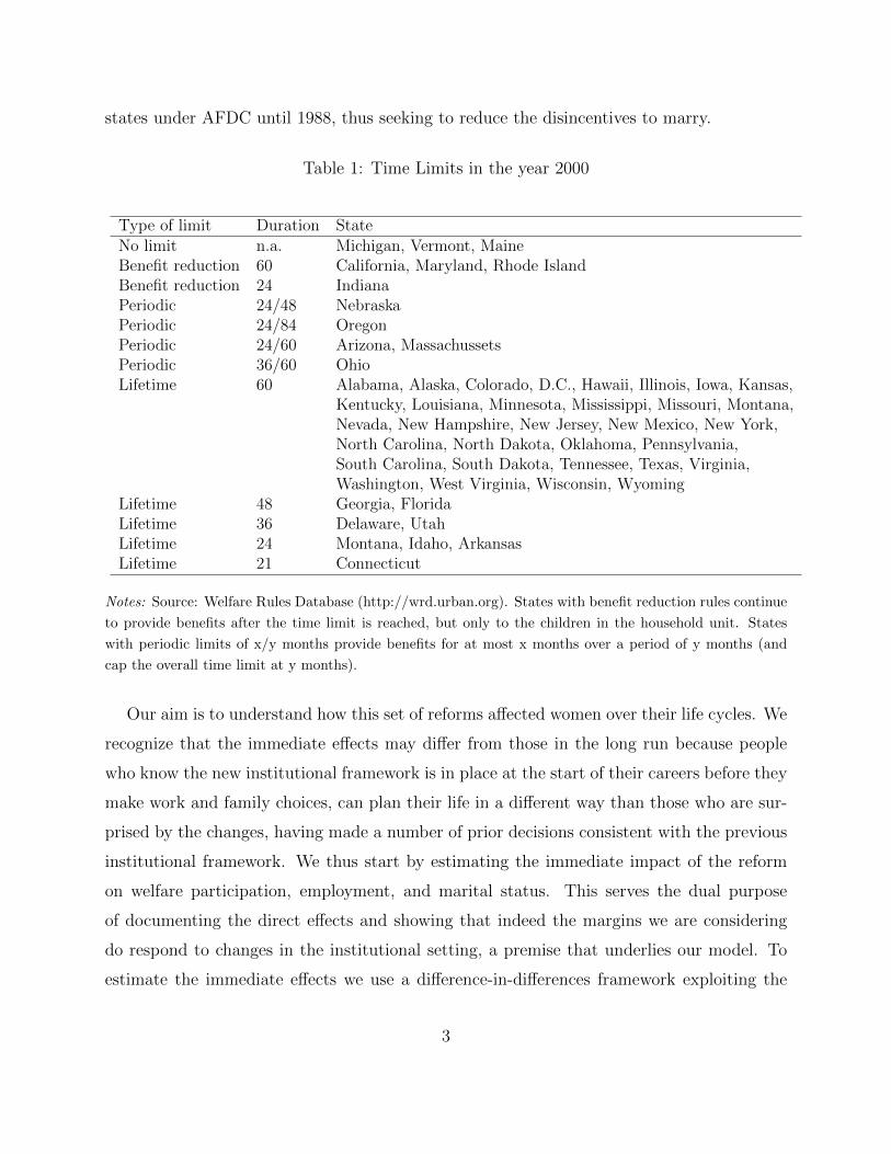
states under AFDC until 1988, thus seeking to reduce the disincentives to marry.

Table 1: Time Limits in the year 2000

Type of limit Duration StateNo limit n.a. Michigan, Vermont, MaineBenefit reduction 60 California, Maryland, Rhode IslandBenefit reduction 24 IndianaPeriodic 24/48 NebraskaPeriodic 24/84 OregonPeriodic 24/60 Arizona, MassachussetsPeriodic 36/60 OhioLifetime 60 Alabama, Alaska, Colorado, D.C., Hawaii, Illinois, Iowa, Kansas,

Kentucky, Louisiana, Minnesota, Mississippi, Missouri, Montana,Nevada, New Hampshire, New Jersey, New Mexico, New York,North Carolina, North Dakota, Oklahoma, Pennsylvania,South Carolina, South Dakota, Tennessee, Texas, Virginia,Washington, West Virginia, Wisconsin, Wyoming

Lifetime 48 Georgia, FloridaLifetime 36 Delaware, UtahLifetime 24 Montana, Idaho, ArkansasLifetime 21 Connecticut

Notes: Source: Welfare Rules Database (http://wrd.urban.org). States with benefit reduction rules continue

to provide benefits after the time limit is reached, but only to the children in the household unit. States

with periodic limits of x/y months provide benefits for at most x months over a period of y months (and

cap the overall time limit at y months).

Our aim is to understand how this set of reforms affected women over their life cycles. We

recognize that the immediate effects may differ from those in the long run because people

who know the new institutional framework is in place at the start of their careers before they

make work and family choices, can plan their life in a different way than those who are sur-

prised by the changes, having made a number of prior decisions consistent with the previous

institutional framework. We thus start by estimating the immediate impact of the reform

on welfare participation, employment, and marital status. This serves the dual purpose

of documenting the direct effects and showing that indeed the margins we are considering

do respond to changes in the institutional setting, a premise that underlies our model. To

estimate the immediate effects we use a difference-in-differences framework exploiting the

3

fact that the new welfare rules varied by state and affected different demographic groups

differently. For example, women whose youngest child is close enough to 18 years old (when

benefit eligibility terminates anyway) would have remained unaffected by the time limits,

while women with younger kids may be affected, depending on the actions taken by their

state of residence. Based on this approach we show that welfare utilization declined quite

dramatically and persistently, employment of women increased, while the flow of divorces

declined, with no detectable effects on the flow of marriages or on fertility.

The reduced form analysis can reliably document the impacts that occurred but cannot

reveal the longer-run dynamics of nor the rich underlying mechanisms through which policy

changes take place. For this purpose we develop a model of female marital and labor supply

choices, which can be used both for understanding the dynamics and the mediating factors

and for counterfactual analysis, leading us to a better understanding of the tradeoffs involved

in designing and reforming welfare programs.

In the model we specify, family formation and dissolution, welfare program participation,

labor supply and savings are endogenous choices. In an attempt to understand better how

welfare reform can affect intrahousehold inequality both in the longer run and the short run

we characterize intrahousehold allocations within a limited commitment framework in which

the outside options of husband and wife are key determinants of both the willingness to marry

and the way resources are allocated within the household. Depending on the circumstances,

the Pareto weights and hence the allocation of resources changes to ensure that the marriage

can continue (if at all possible).

A key element of our approach is the budget constraint and how this is shaped by the

welfare system. We account for the structure of the welfare system that low-income house-

holds are likely to face, including AFDC/TANF, Food Stamps, and the Earned Income Tax

credit (EITC). The full structure, including the budget constraint, allows us to understand

the dynamics implied by the time limits and more generally to evaluate how the structure of

welfare affects marriage, labor supply and the allocation of resources within the household.

We estimate our model using data from the Survey of Income and Program Participation

(SIPP) for the 1990-2011 period using the method of simulated moments (McFadden, 1989;

Pakes and Pollard, 1989). We restrict our sample to women between the ages of 18 and 60

4

who are not college graduates and for whom the policy changes are directly pertinent.

Our paper builds on existing work relating both welfare reform and lifecycle behavior.

The literature on the effects of welfare reform is large and too long to list here. Excellent

overviews are featured in Blank (2002) and Grogger and Karoly (2005). Experimental studies

have highlighted that time limits encourage households to limit benefit utilization to “bank”

their future eligibility (Grogger and Michalopoulos, 2003) and more generally are associated

with reduced welfare participation (Swann, 2005; Mazzolari and Ragusa, 2012).

The literature on employment effects of welfare reform has primarily focused on the sample

of single women (see, for instance, Keane and Wolpin (2010)). This is not surprising, given

that both institutionally and in practice single women with children are the main recipients

and targets of welfare programs such as AFDC or TANF. Recently, Chan (2013) indicates

that time limits associated with welfare reform are an important driver of the increase of labor

supply in this group. Kline and Tartari (forthcoming) examine both intensive and extensive

margin labor supply responses in the context of the Connecticut Jobs First program, which

imposed rather stringent time limits. Limited evidence on the overall effect of welfare reform

on household formation and dissolution suggests that the reform was associated with a small

decline in both marriages and divorces, although the estimated effects tend to be rather

noisy (Bitler et al., 2004).

Our paper draws from the literature on dynamic career models such as Keane and Wolpin

(1997) and subsequent models that allow for savings and labor supply in a family context

such as Blundell et al. (2016). We build on this literature by endogenizing both marriage

and divorce and allowing intra-household allocations to evolve depending on changes in the

economic environment and preferences. The theoretical underpinnings draw from Chiappori

(1988, 1992) and Blundell, Chiappori and Meghir (2005) and its dynamic extension by

Mazzocco (2007b). We apply the risk sharing framework with limited commitment of Ligon,

Thomas and Worrall (2000) and Ligon, Thomas and Worrall (2002b) as extended to the

lifecycle marriage model by Voena (2015).4 Thus we specify a framework that allows us to

4Our paper also relates to the life cycle analyses of female labor supply and marital status (Attanasio, Lowand Sanchez-Marcos, 2008; Fernandez and Wong, 2014; Blundell et al., 2016) and contributes to existingwork on taxes and welfare in a static context including Heckman (1974), Burtless and Hausman (1978),Keane and Moffitt (1998), Eissa and Liebman (1995) for the US as well as Blundell, Duncan and Meghir(1998) for the UK and many others.

5

analyze the way that policy can affect key lifecycle decisions, including marriage, divorce,

savings and labor supply.5

To summarize, our paper offers a number of innovations. First, this is the first model

to endogenize marriage and divorce and to model intrahousehold allocations in a limited

commitment framework, allowing for savings and subject to search frictions in the marriage

market, where people meet potential partners drawn from the empirical distribution of sin-

gles. Second, we do this while taking into account the detailed structure of welfare programs.

Third, we use the short run effects of the reform to validate our model. Finally, we are able

to use our model to estimate the welfare effects of the program and to perform counterfactual

analysis.

In what follows we present first the data and the reduced form analysis of the effects

of the time limits component of the PRWORA. We then discuss our model, followed by

estimation, analysis of the implications and counterfactual policy simulations. We end with

some concluding remarks.

2 The Data and Empirical Evidence on the Effects of

Time Limits

We use eight panels of the Survey of Income and Program Participation (SIPP) spanning

the 1990-2011 period.6 The SIPP is a representative survey of the US population collecting

detailed information on participation in welfare and social insurance programs. In each

panel, people are interviewed every four months for a certain number of times (waves).7 We

restrict the sample to individuals between 18 and 60, with at least one child under age 19,

and who are not college graduates. We focus on low-skilled individuals because they are the

typical recipients of welfare programs. Due to the well-known “seam effect” (Young, 1989),

we keep only the 4th monthly observations for each individual. Table 12 in the Appendix

5See Persson (2014) for an example of how social policy can directly influence household formation.6These are the 1990, 1991, 1992, 1993, 1996, 2001, 2004 and 2008 panels. We do not use the panels

conducted between 1984 and 1989 because during this period most states had categorical exclusion of two-parent households from AFDC. This was changed with the Family Support Act of 1988.

7The number of waves differ by panels. For example, the 1990 panel covers eight waves, while the 1993panel was conducted for nine waves.

6

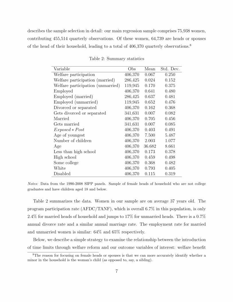
describes the sample selection in detail: our main regression sample comprises 75,938 women,

contributing 455,514 quarterly observations. Of these women, 64,739 are heads or spouses

of the head of their household, leading to a total of 406,370 quarterly observations.8

Table 2: Summary statistics

Variable Obs Mean Std. Dev.Welfare participation 406,370 0.067 0.250Welfare participation (married) 286,425 0.024 0.152Welfare participation (unmarried) 119,945 0.170 0.375Employed 406,370 0.641 0.480Employed (married) 286,425 0.637 0.481Employed (unmarried) 119,945 0.652 0.476Divorced or separated 406,370 0.162 0.368Gets divorced or separated 341,631 0.007 0.082Married 406,370 0.705 0.456Gets married 341,631 0.007 0.085Exposed ∗ Post 406,370 0.403 0.491Age of youngest 406,370 7.500 5.487Number of children 406,370 2.003 1.077Age 406,370 36.682 8.661Less than high school 406,370 0.173 0.378High school 406,370 0.459 0.498Some college 406,370 0.368 0.482White 406,370 0.793 0.405Disabled 406,370 0.115 0.319

Notes: Data from the 1990-2008 SIPP panels. Sample of female heads of household who are not college

graduates and have children aged 18 and below.

Table 2 summarizes the data. Women in our sample are on average 37 years old. The

program participation rate (AFDC/TANF), which is overall 6.7% in this population, is only

2.4% for married heads of household and jumps to 17% for unmarried heads. There is a 0.7%

annual divorce rate and a similar annual marriage rate. The employment rate for married

and unmarried women is similar: 64% and 65% respectively.

Below, we describe a simple strategy to examine the relationship between the introduction

of time limits through welfare reform and our outcome variables of interest: welfare benefit

8The reason for focusing on female heads or spouses is that we can more accurately identify whether aminor in the household is the woman’s child (as opposed to, say, a sibling).

7

utilization, female employment, marital status, and fertility.

2.1 Empirical strategy

The basic idea behind our descriptive empirical strategy is to compare households that,

based on their demographic characteristics and state of residence, could have been affected

by time limits with households that were not affected, before and after time limits were

introduced. This strategy extends prior work about time limits and benefits utilization

(Grogger and Michalopoulos, 2003; Mazzolari and Ragusa, 2012) to a wider set of outcomes,

like labor supply and marital status.

We define a variable Exposed which takes value 0 if the household’s expected benefits have

not changed as a result of the reform, assuming the household has never used benefits before.9

Exposed takes value 1 if a household’s benefits (in terms of eligibility or amounts) have

been affected in any way by the reform. Hence, Exposed is a function of the demographic

characteristics of a household and the rules of the state the household resides (which may

change over time - something we allow for in estimation - both because states differ with

regards to the date where the time limit clock starts to tick and because some states change

their statutory time limits during the sample period).

For example, if a households’s youngest child is aged 13 or above in year t and the state’s

lifetime limit is 60 months, the variable Exposed takes value 0, while if a households’s

youngest child is aged 12 or below in year t and the state’s lifetime limit is 60 months, the

variable Exposed takes value 1.

As well, if a households’s youngest child is aged 13 in year t and the state has a periodic

limit of 24 months every 60, the variable Exposed takes value 1. Lastly, if a households’s

youngest child is aged 16 in year t and the state’s time limit is a periodic limit of 24 months

every 60 months, the variable Exposed takes value 0, because the household would be eligible

for at most 24 months both pre- and post-reform.

9The relationship between our exposure variable and the effect of time limits becomes increasingly at-tenuated as time goes by, since we cannot observe the actual history of welfare utilization. Moreover, inmost states the reform also imposed stricter work requirements, so that a level effect on employment maybe expected across both treated and control groups. However, unless work requirements interact with ageof children in a complex way, our strategy still identifies the differential effect of time limits. Finally, moststates reduce child’s age eligibility to 17 if the child is not in school - a complication we ignore.

8

The estimating equation for household i with demographics d (age of the youngest child)

in state s at time t takes the form:

yidst = αExposeddst ∗ Postst + Xidstβ + fest + feds + fes + fet + fed + εidst

where Postst equals 1 if state s has enacted the reform at time t and 0 otherwise. We

include state, year and demographic (age of the youngest child) fixed effects, as well as state

by time fixed effects to account for differential trends and state by demographic fixed effects

to allow for heterogeneity across states in the way demographic groups behave. Hence, this

exercise can be seen as a difference-in-differences one that compares certain demographic

groups before and after the welfare reform.

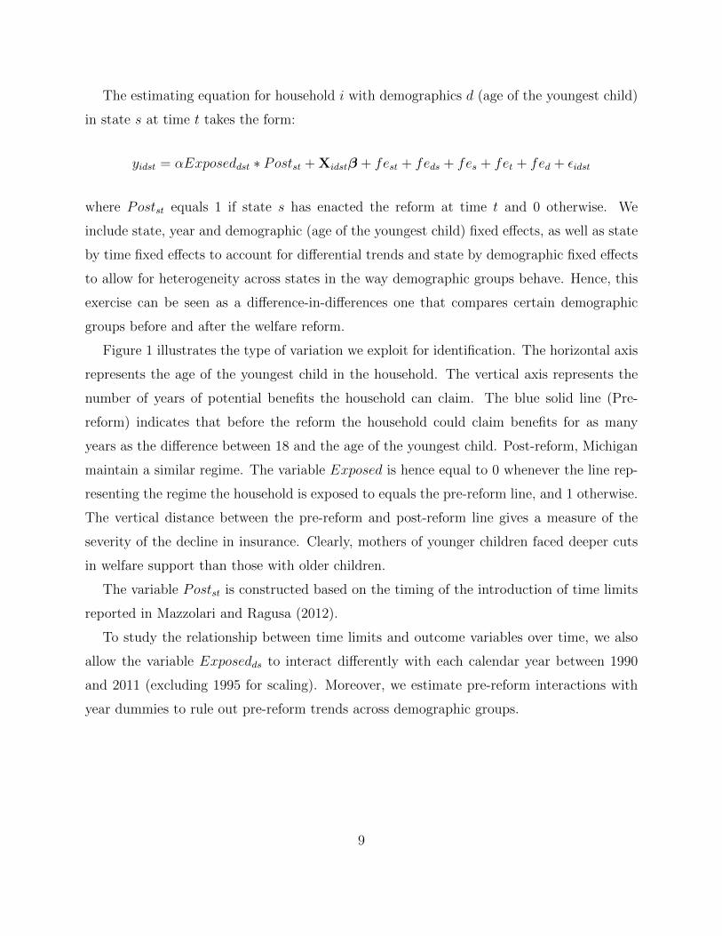
Figure 1 illustrates the type of variation we exploit for identification. The horizontal axis

represents the age of the youngest child in the household. The vertical axis represents the

number of years of potential benefits the household can claim. The blue solid line (Pre-

reform) indicates that before the reform the household could claim benefits for as many

years as the difference between 18 and the age of the youngest child. Post-reform, Michigan

maintain a similar regime. The variable Exposed is hence equal to 0 whenever the line rep-

resenting the regime the household is exposed to equals the pre-reform line, and 1 otherwise.

The vertical distance between the pre-reform and post-reform line gives a measure of the

severity of the decline in insurance. Clearly, mothers of younger children faced deeper cuts

in welfare support than those with older children.

The variable Postst is constructed based on the timing of the introduction of time limits

reported in Mazzolari and Ragusa (2012).

To study the relationship between time limits and outcome variables over time, we also

allow the variable Exposedds to interact differently with each calendar year between 1990

and 2011 (excluding 1995 for scaling). Moreover, we estimate pre-reform interactions with

year dummies to rule out pre-reform trends across demographic groups.

9

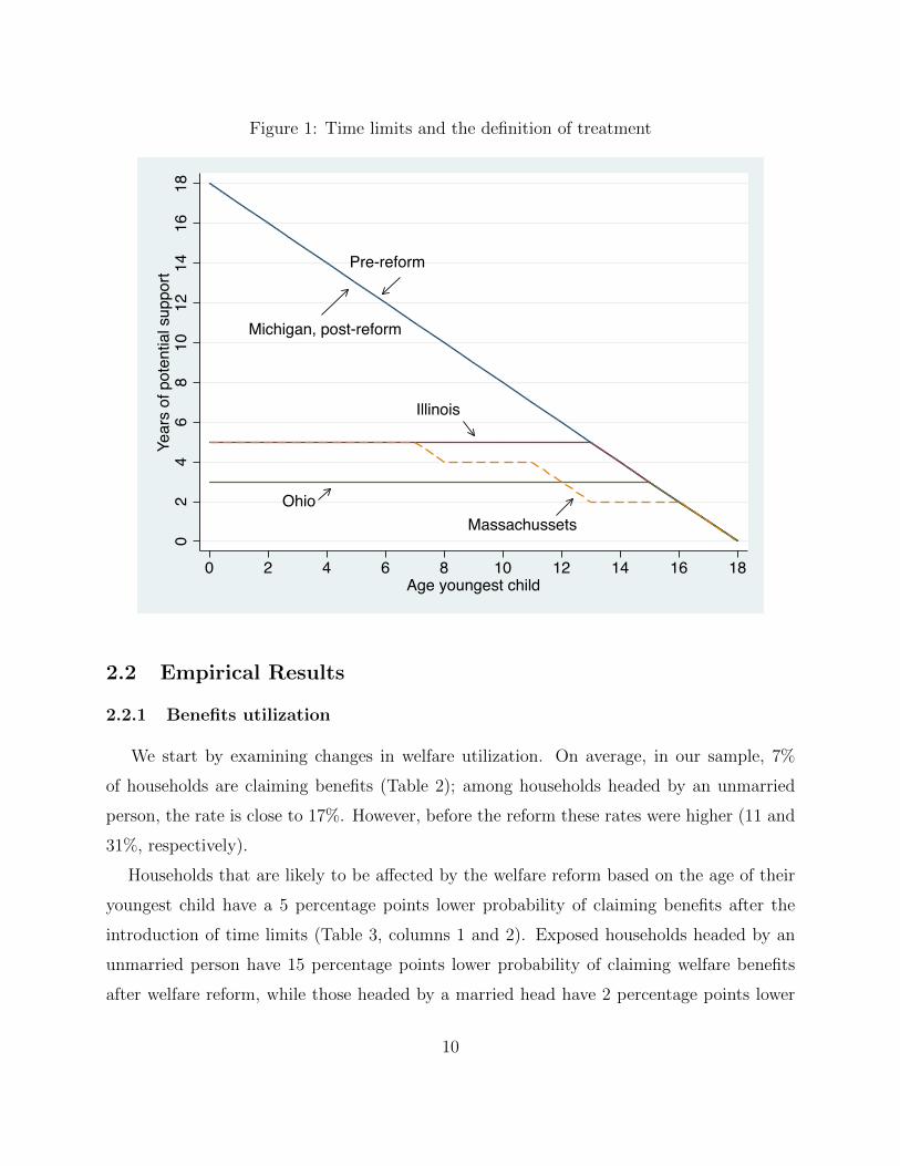
Figure 1: Time limits and the definition of treatment

Pre-reform

Michigan, post-reform

Illinois

OhioMassachussets

02

46

810

1214

1618

Year

s of

pot

entia

l sup

port

0 2 4 6 8 10 12 14 16 18Age youngest child

2.2 Empirical Results

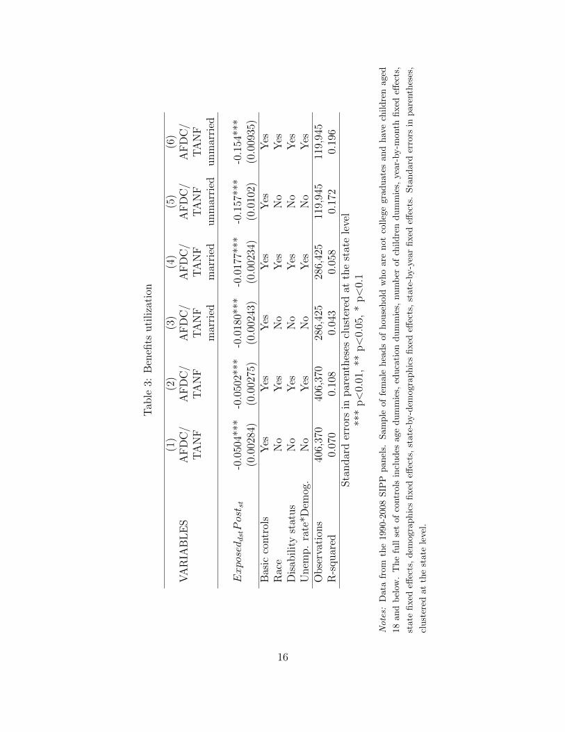
2.2.1 Benefits utilization

We start by examining changes in welfare utilization. On average, in our sample, 7%

of households are claiming benefits (Table 2); among households headed by an unmarried

person, the rate is close to 17%. However, before the reform these rates were higher (11 and

31%, respectively).

Households that are likely to be affected by the welfare reform based on the age of their

youngest child have a 5 percentage points lower probability of claiming benefits after the

introduction of time limits (Table 3, columns 1 and 2). Exposed households headed by an

unmarried person have 15 percentage points lower probability of claiming welfare benefits

after welfare reform, while those headed by a married head have 2 percentage points lower

10

probability of claiming such benefits. The decline among unmarried women is larger for two

reasons: (a) they were the primary participants of the program before the reform, and (b)

they have, on average, younger children, and hence their response should be larger since the

decline in insurance was larger.

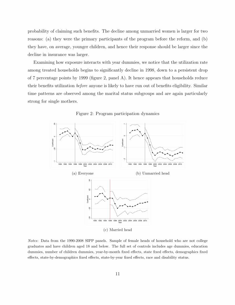
Examining how exposure interacts with year dummies, we notice that the utilization rate

among treated households begins to significantly decline in 1998, down to a persistent drop

of 7 percentage points by 1999 (figure 2, panel A). It hence appears that households reduce

their benefits utilization before anyone is likely to have run out of benefits eligibility. Similar

time patterns are observed among the marital status subgroups and are again particularly

strong for single mothers.

Figure 2: Program participation dynamics

-.1-.05

0.05

Coefficient

1990 1992 1994 1996 1998 2000 2002 2004 2006 2008 2010Year

(a) Everyone

-.2-.1

0.1

Coefficient

1990 1992 1994 1996 1998 2000 2002 2004 2006 2008 2010Year

(b) Unmarried head

-.04

-.02

0.02

.04

Coefficient

1990 1992 1994 1996 1998 2000 2002 2004 2006 2008 2010Year

(c) Married head

Notes: Data from the 1990-2008 SIPP panels. Sample of female heads of household who are not college

graduates and have children aged 18 and below. The full set of controls includes age dummies, education

dummies, number of children dummies, year-by-month fixed effects, state fixed effects, demographics fixed

effects, state-by-demographics fixed effects, state-by-year fixed effects, race and disability status.

11

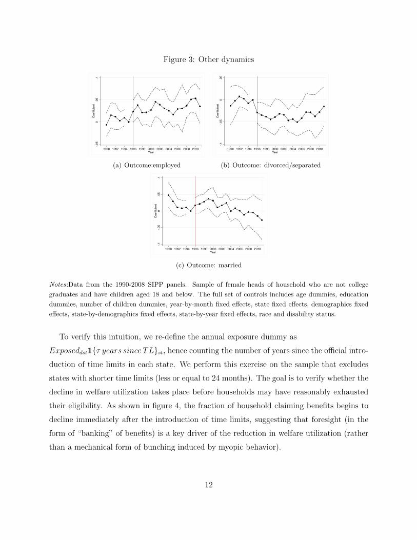
Figure 3: Other dynamics

-.05

0.05

.1Coefficient

1990 1992 1994 1996 1998 2000 2002 2004 2006 2008 2010Year

(a) Outcome:employed

-.1-.05

0.05

Coefficient

1990 1992 1994 1996 1998 2000 2002 2004 2006 2008 2010Year

(b) Outcome: divorced/separated-.1

-.05

0.05

.1Coefficient

1990 1992 1994 1996 1998 2000 2002 2004 2006 2008 2010Year

(c) Outcome: married

Notes:Data from the 1990-2008 SIPP panels. Sample of female heads of household who are not college

graduates and have children aged 18 and below. The full set of controls includes age dummies, education

dummies, number of children dummies, year-by-month fixed effects, state fixed effects, demographics fixed

effects, state-by-demographics fixed effects, state-by-year fixed effects, race and disability status.

To verify this intuition, we re-define the annual exposure dummy as

Exposeddst1τ years since TLst, hence counting the number of years since the official intro-

duction of time limits in each state. We perform this exercise on the sample that excludes

states with shorter time limits (less or equal to 24 months). The goal is to verify whether the

decline in welfare utilization takes place before households may have reasonably exhausted

their eligibility. As shown in figure 4, the fraction of household claiming benefits begins to

decline immediately after the introduction of time limits, suggesting that foresight (in the

form of “banking” of benefits) is a key driver of the reduction in welfare utilization (rather

than a mechanical form of bunching induced by myopic behavior).

12

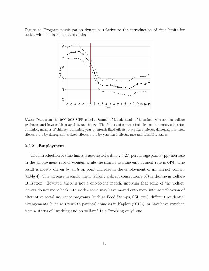
Figure 4: Program participation dynamics relative to the introduction of time limits forstates with limits above 24 months

-.08

-.06

-.04

-.02

0.02

Coefficient

-6 -5 -4 -3 -2 -1 0 1 2 3 4 5 6 7 8 9 10 11 12 13 14 15Time

Notes: Data from the 1990-2008 SIPP panels. Sample of female heads of household who are not college

graduates and have children aged 18 and below. The full set of controls includes age dummies, education

dummies, number of children dummies, year-by-month fixed effects, state fixed effects, demographics fixed

effects, state-by-demographics fixed effects, state-by-year fixed effects, race and disability status.

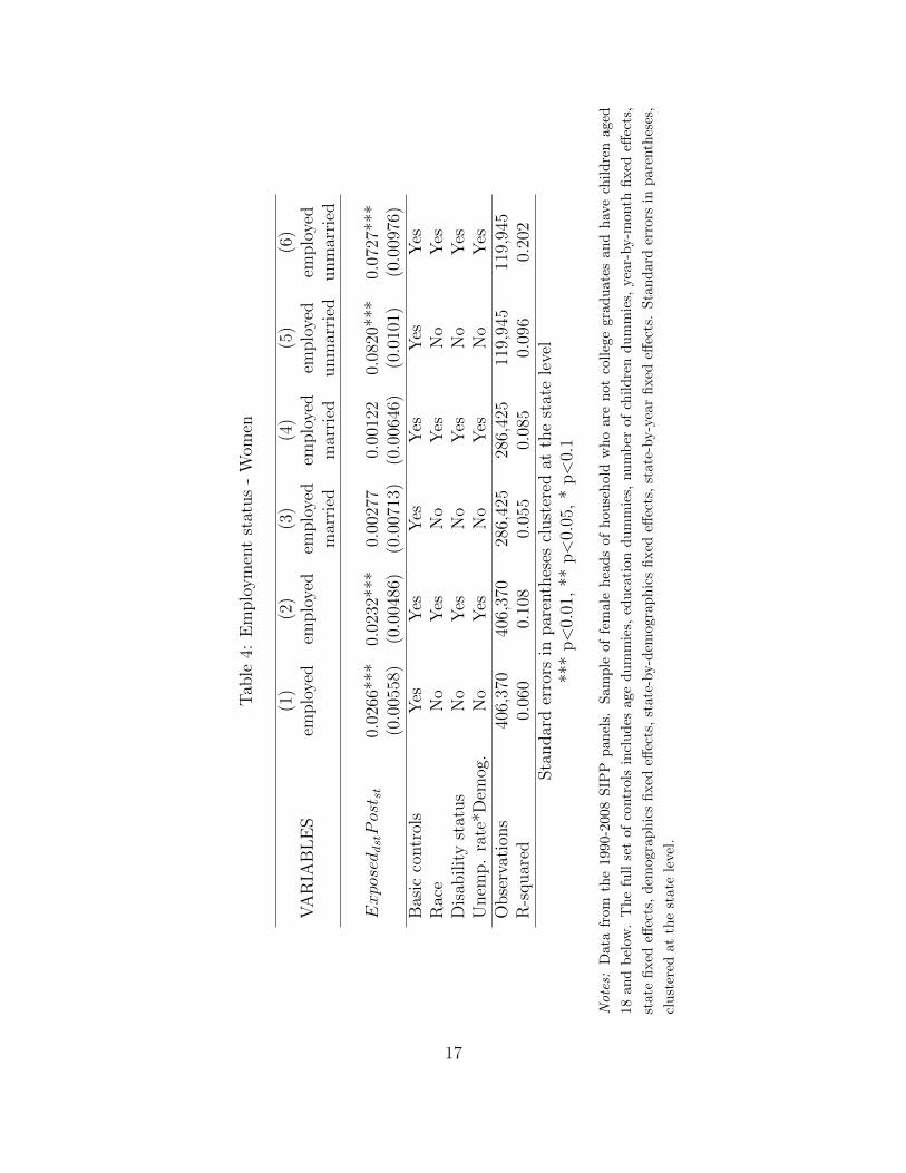
2.2.2 Employment

The introduction of time limits is associated with a 2.3-2.7 percentage points (pp) increase

in the employment rate of women, while the sample average employment rate is 64%. The

result is mostly driven by an 8 pp point increase in the employment of unmarried women.

(table 4). The increase in employment is likely a direct consequence of the decline in welfare

utilization. However, there is not a one-to-one match, implying that some of the welfare

leavers do not move back into work - some may have moved onto more intense utilization of

alternative social insurance programs (such as Food Stamps, SSI, etc.), different residential

arrangements (such as return to parental home as in Kaplan (2012)), or may have switched

from a status of ”working and on welfare” to a ”working only” one.

13

2.2.3 Household formation and dissolution

A central motivation (and indeed a statutory goal) of the 1996 welfare reform was to

encourage “the formation and maintenance of two-parent families”. In studying this rela-

tionship, we first consider the impact of welfare reform on the probability of being divorced

or separated for women. We look both at stocks and flows. We find that treated women are

3 percentage points less likely to be divorced after the introduction of time limits (table 5,

columns 1 and 2). We also find a significant 0.17 percentage points decline in the probabil-

ity of transitioning into divorce conditional on being married during the previous interview

(Table 5, columns 3 and 4). Since on average 0.7 percent of marriages end in divorce at each

interview, this is a non-negligible effect.

As shown in the last two columns of Table 6, the decline in divorce was not associated

with an increase in the fraction of women who are married or who are getting married in

each period.

Thus there seem to be more people staying together but at the same time no change in the

stock of married people, indicating a potential decline in new marriages outside of our sample

of mothers. In theory, as discussed by (Bitler et al., 2004), the effects of the welfare reform

on household formulation and household dissolution are not obvious. The welfare reform, by

curtailing the extent of public insurance available to low-income women, may have induced

those who were already married to attach a higher value to marriage as a valuable risk sharing

tool (through male labor supply, for example). Moreover, the decline in government-provided

insurance reduced the option value of being single (and potentially claiming benefits). On

the marriage side, the demand for insurance through marriage may be counteracted by a

decreasing value of marriage due to the higher financial independence ensured by higher

employment rates. Moroever, the decline in government-provided insurance may have made

single women less attractive in the marriage market.

2.2.4 Fertility

Because our empirical strategy, in this section of the paper, relies on the age of the

youngest child as a source of predetermined variation, it is not suited to examine contempo-

rary changes in fertility outcomes, which directly affect the age of the youngest child. Hence,

14

to examine whether time limits influenced fertility outcomes, we focus on the probability

that a household will have a newborn (a child below age 1) in the following year, with the

specification:

newbornidst+1 = αExposeddst ∗ Postst + Xidstβ + fest + feds + fes + fet + fed + εidst

Appendix table 13 reports the results of estimating this regression on the whole sample

and on subsamples that depend on marital status. In no specification do we find that

exposure to time limits influences the probability of future births, irrespective of marital

status.

15

Tab

le3:

Ben

efits

uti

liza

tion

(1)

(2)

(3)

(4)

(5)

(6)

VA

RIA

BL

ES

AF

DC

/A

FD

C/

AF

DC

/A

FD

C/

AF

DC

/A

FD

C/

TA

NF

TA

NF

TA

NF

TA

NF

TA

NF

TA

NF

mar

ried

mar

ried

unm

arri

edunm

arri

ed

ExposeddstPost st

-0.0

504*

**-0

.050

2***

-0.0

180*

**-0

.017

7***

-0.1

57**

*-0

.154

***

(0.0

0284

)(0

.002

75)

(0.0

0243

)(0

.002

34)

(0.0

102)

(0.0

0935

)B

asic

contr

ols

Yes

Yes

Yes

Yes

Yes

Yes

Rac

eN

oY

esN

oY

esN

oY

esD

isab

ilit

yst

atus

No

Yes

No

Yes

No

Yes

Unem

p.

rate

*Dem

og.

No

Yes

No

Yes

No

Yes

Obse

rvat

ions

406,

370

406,

370

286,

425

286,

425

119,

945

119,

945

R-s

quar

ed0.

070

0.10

80.

043

0.05

80.

172

0.19

6Sta

ndar

der

rors

inpar

enth

eses

clust

ered

atth

est

ate

leve

l**

*p<

0.01

,**

p<

0.05

,*

p<

0.1

Notes:

Dat

afr

omth

e19

90-2

008

SIP

Ppanel

s.S

am

ple

of

fem

ale

hea

ds

of

hou

seh

old

wh

oare

not

coll

ege

gra

du

ate

san

dh

ave

chil

dre

naged

18an

db

elow

.T

he

full

set

ofco

ntr

ols

incl

ud

esage

du

mm

ies,

edu

cati

on

du

mm

ies,

nu

mb

erof

chil

dre

nd

um

mie

s,ye

ar-

by-m

onth

fixed

effec

ts,

stat

efi

xed

effec

ts,

dem

ogra

ph

ics

fixed

effec

ts,

state

-by-d

emogra

ph

ics

fixed

effec

ts,

state

-by-y

ear

fixed

effec

ts.

Sta

nd

ard

erro

rsin

pare

nth

eses

,

clu

ster

edat

the

stat

ele

vel

.

16

Tab

le4:

Em

plo

ym

ent

stat

us

-W

omen

(1)

(2)

(3)

(4)

(5)

(6)

VA

RIA

BL

ES

emplo

yed

emplo

yed

emplo

yed

emplo

yed

emplo

yed

emplo

yed

mar

ried

mar

ried

unm

arri

edunm

arri

ed

ExposeddstPost st

0.02

66**

*0.

0232

***

0.00

277

0.00

122

0.08

20**

*0.

0727

***

(0.0

0558

)(0

.004

86)

(0.0

0713

)(0

.006

46)

(0.0

101)

(0.0

0976

)B

asic

contr

ols

Yes

Yes

Yes

Yes

Yes

Yes

Rac

eN

oY

esN

oY

esN

oY

esD

isab

ilit

yst

atus

No

Yes

No

Yes

No

Yes

Unem

p.

rate

*Dem

og.

No

Yes

No

Yes

No

Yes

Obse

rvat

ions

406,

370

406,

370

286,

425

286,

425

119,

945

119,

945

R-s

quar

ed0.

060

0.10

80.

055

0.08

50.

096

0.20

2Sta

ndar

der

rors

inpar

enth

eses

clust

ered

atth

est

ate

leve

l**

*p<

0.01

,**

p<

0.05

,*

p<

0.1

Notes:

Dat

afr

omth

e19

90-2

008

SIP

Ppanel

s.S

am

ple

of

fem

ale

hea

ds

of

hou

seh

old

wh

oare

not

coll

ege

gra

du

ate

san

dh

ave

chil

dre

naged

18an

db

elow

.T

he

full

set

ofco

ntr

ols

incl

ud

esage

du

mm

ies,

edu

cati

on

du

mm

ies,

nu

mb

erof

chil

dre

nd

um

mie

s,ye

ar-

by-m

onth

fixed

effec

ts,

stat

efi

xed

effec

ts,

dem

ogra

ph

ics

fixed

effec

ts,

state

-by-d

emogra

ph

ics

fixed

effec

ts,

state

-by-y

ear

fixed

effec

ts.

Sta

nd

ard

erro

rsin

pare

nth

eses

,

clu

ster

edat

the

stat

ele

vel

.

17

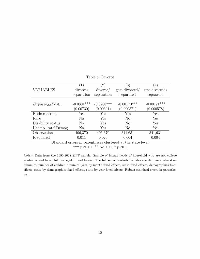
Table 5: Divorce

(1) (2) (3) (4)VARIABLES divorce/ divorce/ gets divorced/ gets divorced/

separation separation separated separated

ExposeddstPostst -0.0301*** -0.0288*** -0.00170*** -0.00171***(0.00730) (0.00691) (0.000571) (0.000578)

Basic controls Yes Yes Yes YesRace No Yes No YesDisability status No Yes No YesUnemp. rate*Demog. No Yes No YesObservations 406,370 406,370 341,631 341,631R-squared 0.011 0.020 0.004 0.004

Standard errors in parentheses clustered at the state level*** p<0.01, ** p<0.05, * p<0.1

Notes: Data from the 1990-2008 SIPP panels. Sample of female heads of household who are not college

graduates and have children aged 18 and below. The full set of controls includes age dummies, education

dummies, number of children dummies, year-by-month fixed effects, state fixed effects, demographics fixed

effects, state-by-demographics fixed effects, state-by-year fixed effects. Robust standard errors in parenthe-

ses.

18

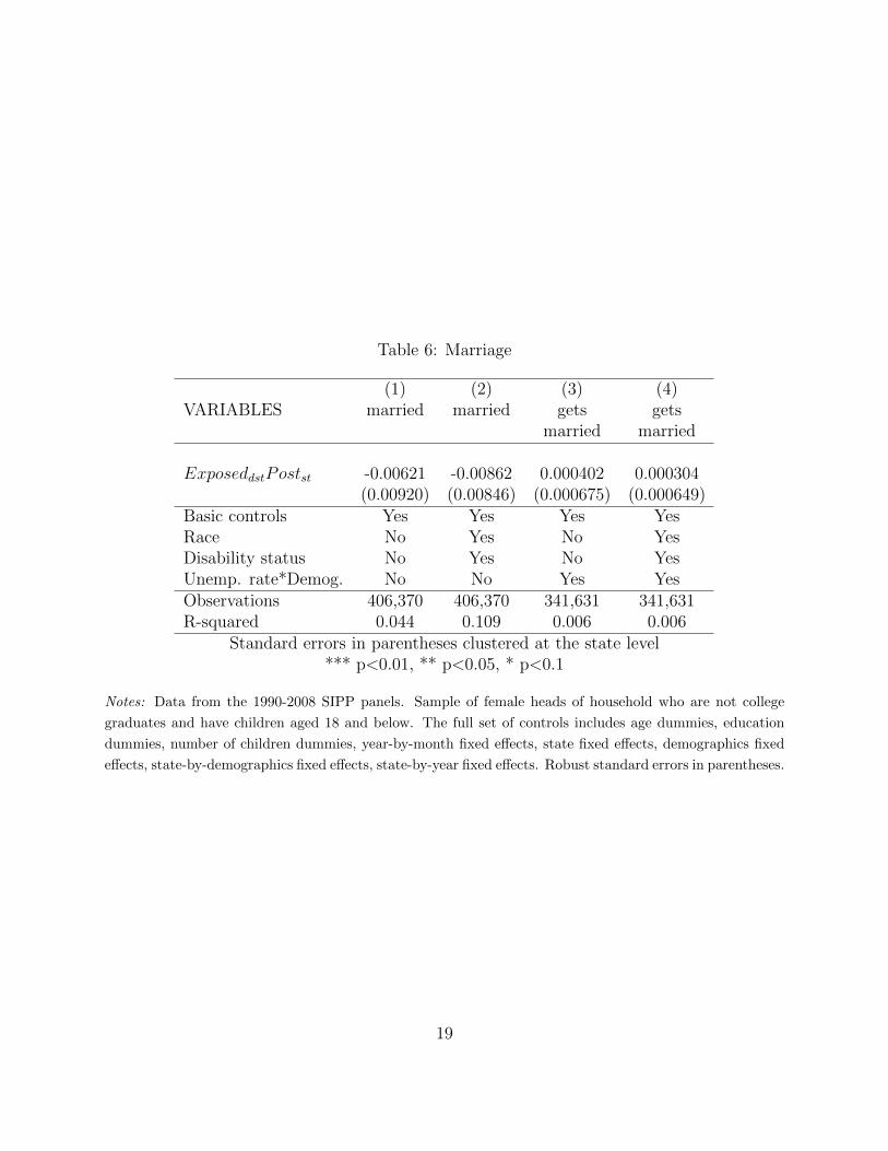
Table 6: Marriage

(1) (2) (3) (4)VARIABLES married married gets gets

married married

ExposeddstPostst -0.00621 -0.00862 0.000402 0.000304(0.00920) (0.00846) (0.000675) (0.000649)

Basic controls Yes Yes Yes YesRace No Yes No YesDisability status No Yes No YesUnemp. rate*Demog. No No Yes YesObservations 406,370 406,370 341,631 341,631R-squared 0.044 0.109 0.006 0.006

Standard errors in parentheses clustered at the state level*** p<0.01, ** p<0.05, * p<0.1

Notes: Data from the 1990-2008 SIPP panels. Sample of female heads of household who are not college

graduates and have children aged 18 and below. The full set of controls includes age dummies, education

dummies, number of children dummies, year-by-month fixed effects, state fixed effects, demographics fixed

effects, state-by-demographics fixed effects, state-by-year fixed effects. Robust standard errors in parentheses.

19

2.3 Robustness checks

To ensure the robustness of our findings, we perform a number of robustness checks.

2.3.1 Attrition in the SIPP sample

To address concerns regarding the high rate of attrition in the SIPP (Zabel, 1998), we

limit our analysis to the first two waves of each SIPP panel. In Appendix table 14 we show

that this adjustment leaves the results unaffected.

2.3.2 College graduates sample

Our sample excludes college graduates because they are unlikely to be targeted by the

reform. To verify this conjecture, we replicate our regressions for welfare use, employment

and marital status using the sameple of college graduates. We find very small effects on

welfare utilization (-0.3pp) and no effects whatsoever on employment and marital status.10

2.3.3 Exclude mothers of young children

A potential concern is that our results are driven by changes in the behavior of households

with small children after welfare reform as a result of the more generous childcare provisions

in the PRWORA.11 Appendix table 15 shows that the results are robust to excluding house-

holds in which the youngest child is below the age of 6. Note that this is a sample where the

decline in welfare benefits is less deep. Not surprisingly (in the light of our model), the em-

ployment effects are smaller than in the whole sample. Another important component of the

1996 welfare reform was the introduction of work requirement. The only threat to identifica-

tion is that work requirement were less stringent for mothers of very young children (below

age one). This should lead our estimates for employment to be downward biased. However,

this is unlikely to represent a significant bias given the size of the population exempted.

10Results available upon request.11The welfare reform eliminated federal child care entitlements and replaced them with a childcare block

grant to the states. Under these changes, states became more flexible in designing their childcare assistanceprograms. In practice, the total amount available for state-level childcare programs could increase or decreasedepending on the state’s own level of investment.

20

2.3.4 Replication in the March CPS data

We use data from the March CPS between 1990 and 2011 to replicate all our main

specifications in the sample that excludes college graduates. As reported in table 17, all

the findings in the SIPP carry through in the CPS: we observe a 3.9pp decline in welfare

participation, concentrated among unmarried women (column 2: -19pp); a 1.5pp increase in

the employment probability, again concentrated among unmarried women (column 4: 12pp);

a substantial decline in the stock and flow of divorces (columns 5 and 6: -2.25pp and -0.025pp

respectively) with no detectable effect on marriage (columns 7 and 8). The dynamics suggest

a substantial amount of benefits banking and an immediate response of all outcome variables

(figure 13).

3 The model

The empirical results above provide support for the hypothesis that low-income house-

holds had an incentive to “bank” their benefits in response to the introduction of time limits.

We also found that women changed their marital decisions (were less likely to terminate their

existing marriages) in response to the reform. This forward-looking behavior is important

for justifying the model we present in this section. The model, while taking into account the

entire family structure, focuses primarily on the behavior of mothers, who can be single or

married. Marriage and divorce are endogenous and take place at the start of the period. We

begin by describing labor supply, savings and welfare participation choices that take place

after the marital status decision. We then describe how marital status choices are made,

and clarify the timing of each shock realization and decision.

3.1 Problem of the single woman

We start by describing the problem of a single woman who has completed her schooling

choices.12 In each period, she decides whether to work, whether to claim welfare and how

12Our main focus in on low-education women, because we are interested in the impacts of means-testedwelfare benefits, such as TANF. An important question is how education choice is itself affected by thepresence of such benefits (Blundell et al., 2016). We leave this question for further research. Bronson(2014) studies women’s education decisions in a dynamic collective model of the household with limited

21

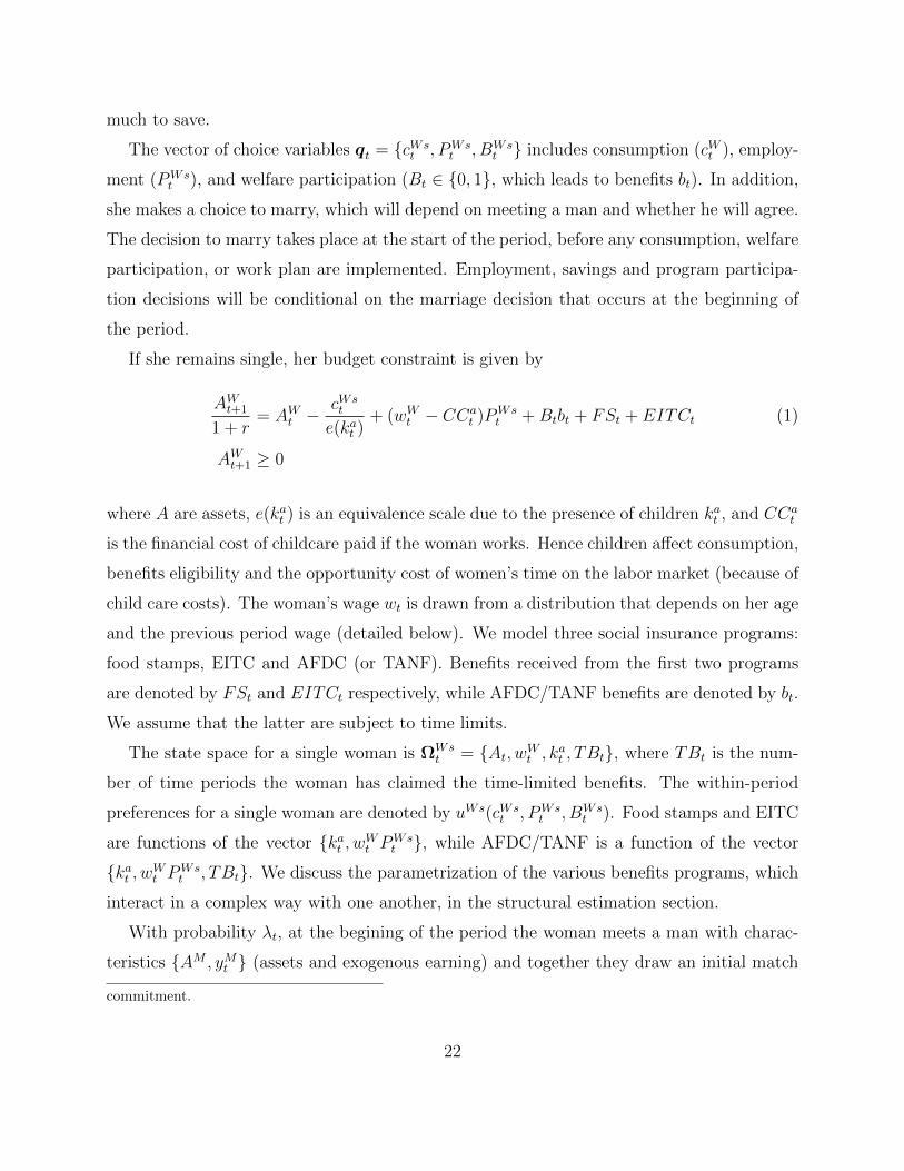
much to save.

The vector of choice variables qt = cWst , PWs

t , BWst includes consumption (cWt ), employ-

ment (PWst ), and welfare participation (Bt ∈ 0, 1, which leads to benefits bt). In addition,

she makes a choice to marry, which will depend on meeting a man and whether he will agree.

The decision to marry takes place at the start of the period, before any consumption, welfare

participation, or work plan are implemented. Employment, savings and program participa-

tion decisions will be conditional on the marriage decision that occurs at the beginning of

the period.

If she remains single, her budget constraint is given by

AWt+1

1 + r= AWt −

cWst

e(kat )+ (wWt − CCa

t )PWst +Btbt + FSt + EITCt (1)

AWt+1 ≥ 0

where A are assets, e(kat ) is an equivalence scale due to the presence of children kat , and CCat

is the financial cost of childcare paid if the woman works. Hence children affect consumption,

benefits eligibility and the opportunity cost of women’s time on the labor market (because of

child care costs). The woman’s wage wt is drawn from a distribution that depends on her age

and the previous period wage (detailed below). We model three social insurance programs:

food stamps, EITC and AFDC (or TANF). Benefits received from the first two programs

are denoted by FSt and EITCt respectively, while AFDC/TANF benefits are denoted by bt.

We assume that the latter are subject to time limits.

The state space for a single woman is ΩWst = At, wWt , kat , TBt, where TBt is the num-

ber of time periods the woman has claimed the time-limited benefits. The within-period

preferences for a single woman are denoted by uWs(cWst , PWs

t , BWst ). Food stamps and EITC

are functions of the vector kat , wWt PWst , while AFDC/TANF is a function of the vector

kat , wWt PWst , TBt. We discuss the parametrization of the various benefits programs, which

interact in a complex way with one another, in the structural estimation section.

With probability λt, at the begining of the period the woman meets a man with charac-

teristics AM , yMt (assets and exogenous earning) and together they draw an initial match

commitment.

22

quality L0t . In the case a meeting occurs, the two individuals decide whether to get married,

as described below. Denote the distribution of available men in period t as G(A, y|t). We

restrict encounters to be between a man and a woman of the same age group.13

We denote by V Wst (ΩWs

t ) the value function for a single woman at age t and V Wmt (ΩWm

t )

the value function for a married woman at age t, which we will define below.

A single woman has the following value functions:

V Wst (ΩWs

t ) = maxqtuWs(cWs

t , PWst , BWs

t )

+βEt[λt+1[(1−mt+1(Ωt+1))V

Wst+1 (ΩWs

t+1) +mt+1(Ωt+1)VWmt+1 (Ωm

t+1)] + (1− λt+1)VWst+1 (ΩWs

t+1)]

subject to the two constraints in (1), and where mt+1 represents a dummy for marrying in

period t+ 1.

3.2 Problem of the single man

Men solve an analogous problem without welfare benefits and without a labor supply

choice. Men’s earnings follow a stochastic process described by the distribution fM(yMt |yMt−1, t).Children affect the man’s problem only when he is married to their mother.

These assumptions determine V Ms(ΩMst ), the man’s value function when he is single.

V Mmt (ΩM

t ) is the value accruing to a married man. In all cases ΩMt is the relevant state

space.

His budget constraint is given by14

AMt+1

1 + r= AMt − cMs

t + yMt + FSt (2)

AMt+1 ≥ 0.

13In principle, this distribution is endogenous and as economic conditions change, the associated marriagemarket will change, with this “offer” distribution changing. In this paper we take this distribution as givenand do not solve for it endogenously. This mainly affects counterfactual simulations. Note that solving forthe equilibrium distribution in two dimensions is likely to be very complicated computationally.

14We do not consider EITC for men because the value of the program for an individual without a qualifyingchild is modest (for example, in 2017 the maximum annual credit for an individual without a qualifying childwas $510, as opposed to $3,400 for those with a qualifying child).

23

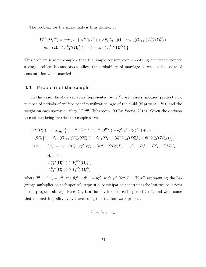
The problem for the single male is thus defined by

V Mst (ΩMs

t ) = maxcMtuMs(cMs

t ) + βEt[λt+1[(1−mt+1(Ωt+1))VMst+1 (ΩMs

t+1)

+mt+1(Ωt+1)VMmt+1 (ΩM

t+1)] + (1− λt+1)VMst+1 (ΩMs

t+1)].

This problem is more complex than the simple consumption smoothing and precautionary

savings problem because assets affect the probability of marriage as well as the share of

consumption when married.

3.3 Problem of the couple

In this case, the state variables (represented by Ωmt ), are: assets, spouses’ productivity,

number of periods of welfare benefits utilization, age of the child (if present) (kat ), and the

weight on each spouse’s utility θHt , θWt (Mazzocco, 2007a; Voena, 2015). Given the decision

to continue being married the couple solves:

V mt (Ωm

t ) = maxqtθWt uWm(cWm

t , PWmt , BWm

t ) + θMt uMm(cMmt ) + Lt

+βEt[(1− dt+1(Ωt+1))V

mt+1(Ω

mt+1) + dt+1(Ωt+1)

(θWt V

Wst+1 (ΩWs

t+1) + θMt VMst+1 (ΩMs

t+1))]

s.t. At+1

1+r= At − x(cWt , c

Mt , k

at ) + (wWt − CCa

t )PWt + yMt +Btbt + FSt + EITCt

At+1 ≥ 0

V Wmt+1 (Ωm

t+1) ≥ V Wst+1 (ΩWs

t+1)

V Mmt+1 (Ωm

t+1) ≥ V Mst+1 (ΩMs

t+1)

where θWt = θWt−1 + µWt and θMt = θMt−1 + µMt , with µJt (for J = W,M) representing the La-

grange multiplier on each spouse’s sequential participation constraint (the last two equations

in the program above). Here dt+1 is a dummy for divorce in period t + 1, and we assume

that the match quality evolves according to a random walk process:

Lt = Lt−1 + ξt

24

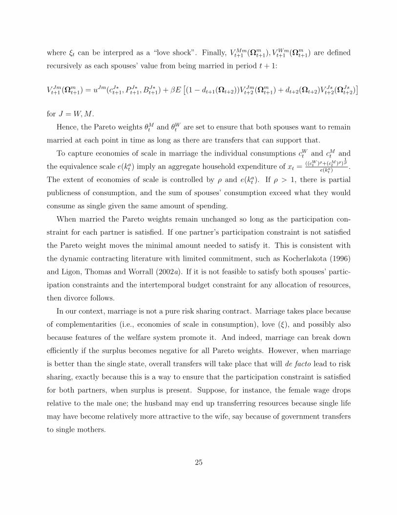
where ξt can be interpred as a “love shock”. Finally, V Mmt+1 (Ωm

t+1), VWmt+1 (Ωm

t+1) are defined

recursively as each spouses’ value from being married in period t+ 1:

V Jmt+1 (Ωm

t+1) = uJm(cJ∗t+1, PJ∗t+1, B

J∗t+1) + βE

[(1− dt+1(Ωt+2))V

Jmt+2 (Ωm

t+1) + dt+2(Ωt+2)VJst+2(Ω

Jst+2)]

for J = W,M .

Hence, the Pareto weights θMt and θWt are set to ensure that both spouses want to remain

married at each point in time as long as there are transfers that can support that.

To capture economies of scale in marriage the individual consumptions cWt and cMt and

the equivalence scale e(kat ) imply an aggregate household expenditure of xt =((cWt )ρ+(cMt )ρ)

1ρ

e(kat ).

The extent of economies of scale is controlled by ρ and e(kat ). If ρ > 1, there is partial

publicness of consumption, and the sum of spouses’ consumption exceed what they would

consume as single given the same amount of spending.

When married the Pareto weights remain unchanged so long as the participation con-

straint for each partner is satisfied. If one partner’s participation constraint is not satisfied

the Pareto weight moves the minimal amount needed to satisfy it. This is consistent with

the dynamic contracting literature with limited commitment, such as Kocherlakota (1996)

and Ligon, Thomas and Worrall (2002a). If it is not feasible to satisfy both spouses’ partic-

ipation constraints and the intertemporal budget constraint for any allocation of resources,

then divorce follows.

In our context, marriage is not a pure risk sharing contract. Marriage takes place because

of complementarities (i.e., economies of scale in consumption), love (ξ), and possibly also

because features of the welfare system promote it. And indeed, marriage can break down

efficiently if the surplus becomes negative for all Pareto weights. However, when marriage

is better than the single state, overall transfers will take place that will de facto lead to risk

sharing, exactly because this is a way to ensure that the participation constraint is satisfied

for both partners, when surplus is present. Suppose, for instance, the female wage drops

relative to the male one; the husband may end up transferring resources because single life

may have become relatively more attractive to the wife, say because of government transfers

to single mothers.

25

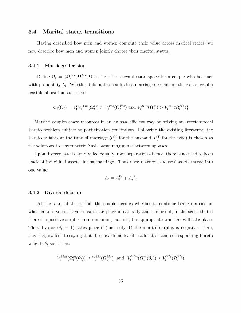
3.4 Marital status transitions

Having described how men and women compute their value across marital states, we

now describe how men and women jointly choose their marital status.

3.4.1 Marriage decision

Define Ωt = ΩWst ,ΩMs

t ,Ωmt , i.e., the relevant state space for a couple who has met

with probability λt. Whether this match results in a marriage depends on the existence of a

feasible allocation such that:

mt(Ωt) = 1V Wmt (Ωm

t ) > V Wst (ΩWs

t ) and V Mmt (Ωm

t ) > V Mst (ΩMs

t )

Married couples share resources in an ex post efficient way by solving an intertemporal

Pareto problem subject to participation constraints. Following the existing literature, the

Pareto weights at the time of marriage (θM1 for the husband, θW1 for the wife) is chosen as

the solutions to a symmetric Nash bargaining game between spouses.

Upon divorce, assets are divided equally upon separation - hence, there is no need to keep

track of individual assets during marriage. Thus once married, spouses’ assets merge into

one value:

At = AWt + AMt .

3.4.2 Divorce decision

At the start of the period, the couple decides whether to continue being married or

whether to divorce. Divorce can take place unilaterally and is efficient, in the sense that if

there is a positive surplus from remaining married, the appropriate transfers will take place.

Thus divorce (dt = 1) takes place if (and only if) the marital surplus is negative. Here,

this is equivalent to saying that there exists no feasible allocation and corresponding Pareto

weights θt such that:

V Mmt (Ωm

t (θt)) ≥ V Mst (ΩMs

t ) and V Wmt (Ωm

t (θt)) ≥ V Wst (ΩWs

t )

26

where θt is a vector of the two Pareto weights in period t discussed below. The value

functions for being single are defined above and evaluated at the level of assets implied by

the equal division of assets as defined in divorce law.

3.5 Exogenous processes

3.5.1 Fertility

Children arrive exogenously, given marital status. The conditional probability of having

a child is taken to be Pr(k1t |mt−1, t). The maximum number of children is 1. The probability

depends on whether a male partner is present (m = 1), and hence to some extent fertility is

endogenous through the marital decision.

3.5.2 Female wages and male earnings

We estimate an hourly wage process for the woman and an earnings process for the

men. Since we take female employment as endogenous we also need to control for selection.

However, we simplify the overall estimation problem by estimating the income processes

separately and outside the model. The woman’s average hourly earnings is obtained by

dividing total earnings by total hours.15

The earnings process for men and the wage process for women take the form

log(yMit ) = aM0 + aM1 t+ aM2 t2 + zMit + εMit

log(wWit ) = aW0 + aW1 t+ aW2 t2 + zWit + εWit

zMit = zMi,t−1 + ζMit

zWit = zWi,t−1 + ζWit .

for j = H,M , zJit is permanent income, which evolves as a random walk following innovation

ζJit, and εJit is i.i.d. measurement error.16

15We take the sum of earnings and hours worked to construct the average hourly earning. For the rest ofthe variables, we consider the last observation within a year.

16One interesting issue is the extent to which the reform affected the labor market and in particular human

27

3.6 Timing

At the beginning of each period, uncertainty is realized. People observe their productivity

realization ζJt and childless women learn whether they have a child, as a function of their

marital status at the beginning of the period. If single, people may meet a partner drawn

from the distribution of singles and observe both the partner’s characteristics and an initial

match quality L0. If they are married, they observe the realization of the match quality

shock ξτ .

Based on these state variables, marital status and the sharing rule are jointly decided.

Conditional on a marital status and on a sharing rule for couples, consumption, labor supply

and program participation choices are made, which determine the state variables in the

following period.

4 Estimation of model parameters

We choose the parameters of the model using a multi-step approach. Some parameters

(such as risk aversion) are selected from outside the model, using standard values in the

literature. Other parameters are estimated from the data, but without imposing the model’s

structure. The remaining parameters are estimated using the method of simulated moments,

matching data and model-based simulated moments. Since our model starts at age 21, but

by that age some women have already experienced marriage, divorce or childbirth, we impose

some initial conditions directly from the data. Table 9 summarizes the parameters of the

model. We first describe our parametrization choices, then explain the estimation procedures

more in detail.

capital prices (Rothstein, 2010). Whether such general equilibrium effects are important or not depends verymuch on the extent to which the skills of those affected by the welfare reforms are substitutable or otherwisewith respect to the rest of the population. With reasonable amounts of substitutability we do not expectimportant general equilibrium effects.

28

4.1 Parametrization

4.1.1 Preferences

A woman’s within-period utility function is

u(c, P,B) =

(c · eψ(M,ka)·P )1−γ

1− γ− ηB.

In the above, when a person works (P = 1) her marginal utility of consumption (c) changes,

by an amount that depends on the presence of a child. The parameter η represents the

stigma cost from claiming AFDC/TANF benefits.17

4.1.2 Partner meeting process

Couples meet with probability λt. We parametrize λt to vary over time according to the

following rule:

λt = minmaxλ0 + λ1 · t+ λ2 · t2, 0, 1.

When two individuals meet, they draw an initial match quality Lt0 from a distribution

N(0, σ20). If marriage occurs, match quality then evolves as a random walk for married

couples as:

Lt0+τ = Lt0+τ−1 + ξτ

where t0 is the time of marriage, τ are the years of marriage and the innovations ξτ follow

a distribution N(0, σ2ξ ). Hence, we allow the distribution of the initial match quality draw

and the one of the subsequent innovations to differ.

17We assume there is no stigma cost from claiming Food Stamps or EITC benefits - this is because forthese two programs we do not endogenize the participation decision.

29

4.2 Estimation: Selected parameters

As reported in Panel A of Table 9, we set the coefficient of reative risk aversion to 1.5 and

the discount rate to 0.98, values that are relatively uncontroversial. We set the parameter

defining economies of scale in marriage from Voena (2015).

4.3 Estimation: Exogenous processes

4.3.1 Childcare costs

We estimate childcare cost using information from the Consumer Expenditure Survey for

the 1990-1996 period. We sum spending on babysitting and day care and then compute

averages for working women, separately by marital status and age of the child.

4.3.2 Welfare program parameters

We model the welfare system by considering AFDC/TANF, food stamps and EITC ben-

efits. Eligibility for these benefits is based on a combination of economic and demographic

criteria.

AFDC and TANF benefits amounts are established for different household compositions

and household income levels by taking an average benefit level across states, weighted by

the states’ population. In our model, all adult earnings determine income eligibility for

AFDC/TANF. Figure 5 shows how AFDC benefits vary by income level and by marital

status. A single mother with no sources of income receives approximately $315 per month

in AFDC benefits. Adopting the OECD equivalence scale, the adult equivalent amount is

approximately $210. If she were to marry a man with no income, benefits would increase,

but less than what would be needed to keep her adult equivalent amount unchanged.

Similarly, we include food stamps by taking an average of food stamps amounts by differ-

ent household compositions and household income levels (we ignore state variation because

food stamps is a federal program). Unlike AFDC or TANF, food stamps are available to all

households, irrespective of the presence and of the age of the children. Eligibility and amount

of food stamp benefits are determined by accounting for adult earnings and for AFDC or

TANF benefits, which generate household income, as well as household assets.

30

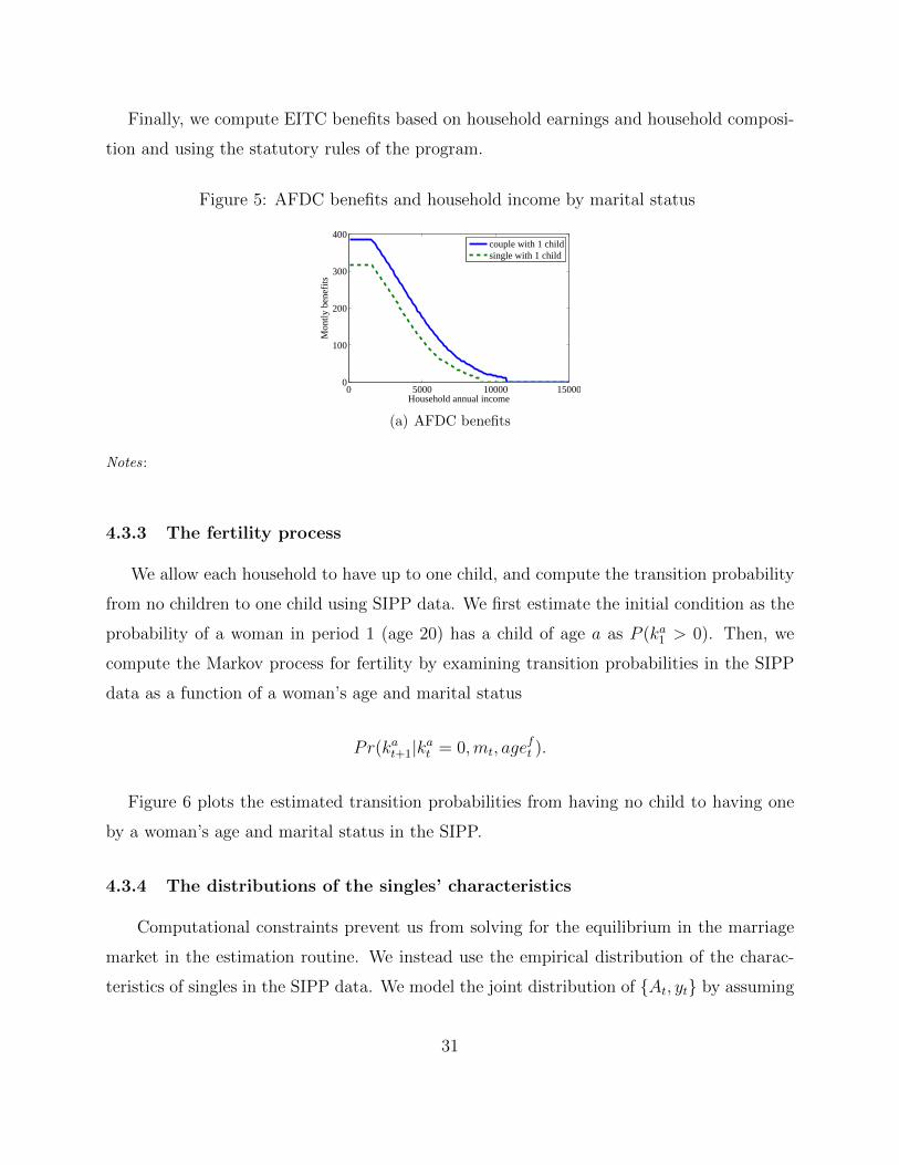
Finally, we compute EITC benefits based on household earnings and household composi-

tion and using the statutory rules of the program.

Figure 5: AFDC benefits and household income by marital status

0 5000 10000 150000

100

200

300

400

Household annual income

Mon

tly b

enef

its

couple with 1 childsingle with 1 child

(a) AFDC benefits

Notes:

4.3.3 The fertility process

We allow each household to have up to one child, and compute the transition probability

from no children to one child using SIPP data. We first estimate the initial condition as the

probability of a woman in period 1 (age 20) has a child of age a as P (ka1 > 0). Then, we

compute the Markov process for fertility by examining transition probabilities in the SIPP

data as a function of a woman’s age and marital status

Pr(kat+1|kat = 0,mt, ageft ).

Figure 6 plots the estimated transition probabilities from having no child to having one

by a woman’s age and marital status in the SIPP.

4.3.4 The distributions of the singles’ characteristics

Computational constraints prevent us from solving for the equilibrium in the marriage

market in the estimation routine. We instead use the empirical distribution of the charac-

teristics of singles in the SIPP data. We model the joint distribution of At, yt by assuming

31

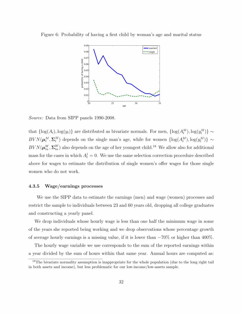
Figure 6: Probability of having a first child by woman’s age and marital status

20 25 30 350

0.01

0.02

0.03

0.04

0.05

0.06

0.07

0.08

0.09

age

prob

abili

ty o

f hav

ing

a ch

ild

marriedsingle

Source: Data from SIPP panels 1990-2008.

that log(At), log(yt) are distributed as bivariate normals. For men, log(AMt ), log(yMt ) ∼BV N(µMt ,Σ

Mt ) depends on the single man’s age, while for women log(AMt ), log(yMt ) ∼

BV N(µWta ,ΣWta ) also depends on the age of her youngest child.18 We allow also for additional

mass for the cases in which Ajt = 0. We use the same selection correction procedure described

above for wages to estimate the distribution of single women’s offer wages for those single

women who do not work.

4.3.5 Wage/earnings processes

We use the SIPP data to estimate the earnings (men) and wage (women) processes and

restrict the sample to individuals between 23 and 60 years old, dropping all college graduates

and constructing a yearly panel.

We drop individuals whose hourly wage is less than one half the minimum wage in some

of the years she reported being working and we drop observations whose percentage growth

of average hourly earnings is a missing value, if it is lower than −70% or higher than 400%.

The hourly wage variable we use corresponds to the sum of the reported earnings within

a year divided by the sum of hours within that same year. Annual hours are computed as:

18The bivariate normality assumption is inappropriate for the whole population (due to the long right tailin both assets and income), but less problematic for our low-income/low-assets sample.

32

reported weekly “usual hours of work” × the number of weeks at the job within the month

× number of months the individual reported positive earnings.

For men, we compute GMM estimates of the variance of the permanent component of log

income (σ2ζ ) and the variance of the measurement error (σ2

ε), based on the following moment

conditions:

E[∆u2t ] = σ2ζ + 2σ2

ε

E[∆ut∆ut−1] = −σ2ε

where ut is the residual log earnings obtained after regressing earnings on dummy for age,

disability status, and year.

For women, we need to address selection into employment, and we do so by implementing

a two-step Heckman selection correction procedure. Wages are:

logwit = Xitβ + εit. (3)

In Xit we include age dummies, disability status, race, state dummies and year dummies.

Wages are observed only when the woman works (Pit = 1), which happens under the following

condition:

Zitγ + νit > 0,

where wit is annual earnings. In Zit we include Xit and a vector of instruments. These

instruments are ”simulated” welfare benefits, as described in Low and Pistaferri (2015)

Appendix C. In particular, we use state, year and demographic variation in simulated AFDC,

EITC and food stamps benefits for a single mother with varying number of children who

works part-time at the minimum wage. The first stage is reported in table 7.

We use the selection correction to estimate the profile of a woman’s wage and to correct

the residuals from estimating equation 3 to estimate the variance of women’s productivity

shocks. GMM estimates of the variance of the permanent component of log income (σ2ζ ) are

33

computed based on the following moment conditions:

E[∆ut | Pt = 1, Pt−1 = 1] = σζW η

[φ(αt)

1− Φ(αt)

]E[∆u2t | Pt = 1, Pt−1 = 1] = σ2

ζW + σ2ζW η

[φ(αt)

1− Φ(αt)αt

]+ 2σ2

εW

E[∆ut∆ut−1 | Pt = 1, Pt−1 = 1, Pt−2 = 1] = −σ2εW

where αt = −Ztγ and where we ignore selection correction for the first order covariance in

order to reduce noise.

Table 7: Employment status Probit regressions - Women

(1) (2)VARIABLES coeff. marg. eff.

Average AFDC payment ($100) -0.064*** -0.021***(0.007) (0.003)

Average food stamps payment ($100) -0.002 -0.008(0.095) (0.031)

Average EITC payment ($100) 0.183*** 0.060***(0.054) (0.018)

Age dummies YesState dummies YesYear dummies YesControls YesObservations 69,832

Standard errors in parentheses*** p<0.01, ** p<0.05, * p<0.1

Notes: Data from the 1990-2008 SIPP panels. Sample of non-college graduates. Annualized data.

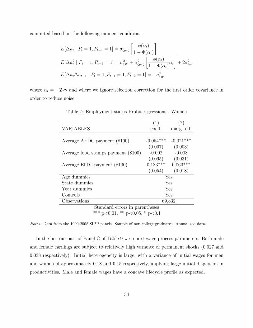
In the bottom part of Panel C of Table 9 we report wage process parameters. Both male

and female earnings are subject to relatively high variance of permanent shocks (0.027 and

0.038 respectively). Initial heterogeneity is large, with a variance of initial wages for men

and women of approximately 0.18 and 0.15 respectively, implying large initial dispersion in

productivities. Male and female wages have a concave lifecycle profile as expected.

34

4.4 Estimation: Method of Simulated Moments

We estimate the remaining parameters of model by the Method of Simulated Moments

(McFadden, 1989):

minΠ(φdata − φsim(Π))G(φdata − φsim(Π))′. (4)

The vector Π contains the following parameters: the disutility from working parameters

for unmarried women without children (ψ00), married women without children (ψ01), women

with a child (ψ11), and unmarried women with a child (ψ10); the variance of match quality

at marriage (σ20); the variance of innovations to match quality (σ2

ξ ); the parameters charac-

terizing the probability of meeting a partner over the life cycle (λ0, λ1, λ2); and the stigma

cost of being on welfare (η).

We estimate our empirical moments φdata on the SIPP sample of women without a college

degree. We focus on the 1960-69 birth cohort in the pre-reform period (1990-95).19 These

women are between age 21 and 35, ages for which we have a sufficiently large number of

observations. We annualize data by considering the marital status, fertility, employment

status and welfare participation status that women had for more than half of the calendar

year. We use a the variance-covariance matrix of the empirical moments as weighting matrix

G, computed using the bootstrap method.

We consider three sets of moments, listed in table 8. The first set of moments includes

conditional moments for labor supply, i.e., the fraction of women employed by marital and

fertility status (which pin down the disutility from work for the different types) and the

proportion of single mothers on welfare (which identifies the stigma cost from welfare par-

ticipation). The second set of moment includes the profile of the probability of being ever

married between age 21 and age 35. These moments jointly contribute to pinning down the

variance of initial match quality, as well as the parameters characterizing the probability of

meeting a potential partner. The third sets of moments includes the probability of divorcing

between age 26 and age 35. The reason why we do not consider these moments for earlier

19We use pre-reform data for three reasons. First, the model is easier to solve when we do not have to keeptrack of the time in the past spent on welfare. Second, we can use post-reform data to validate the model.Finally, in the post-reform period it is difficult to separately identify reluctance to participate in welfare dueto stigma from “banking” behavior.

35

ages is related to initial conditions: divorces in these early years are concentrated among

people who married before age 21, for which we do not know the actual distribution of the

match quality realizations, as the marriages occur before the model begins. These moments

mostly pin down the variance of the initial draw and of the innovations to match quality.

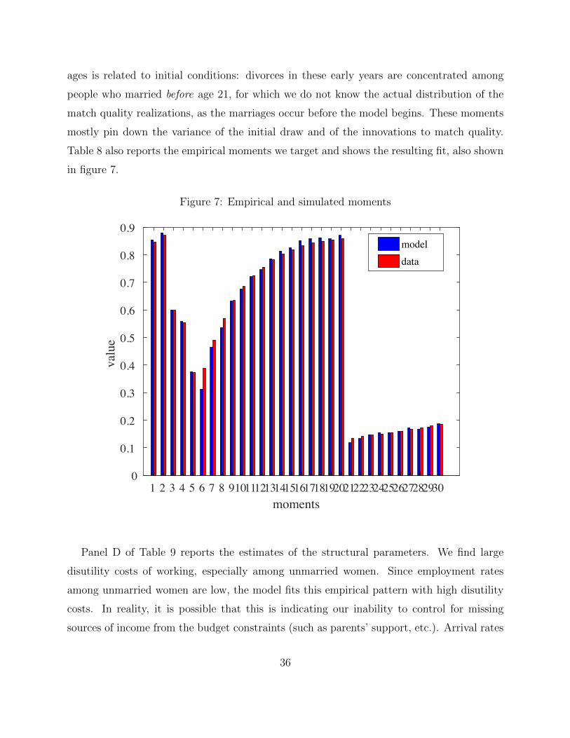
Table 8 also reports the empirical moments we target and shows the resulting fit, also shown

in figure 7.

Figure 7: Empirical and simulated moments

1 2 3 4 5 6 7 8 9101112131415161718192021222324252627282930moments

0

0.1

0.2

0.3

0.4

0.5

0.6

0.7

0.8

0.9

value

modeldata

Panel D of Table 9 reports the estimates of the structural parameters. We find large

disutility costs of working, especially among unmarried women. Since employment rates

among unmarried women are low, the model fits this empirical pattern with high disutility

costs. In reality, it is possible that this is indicating our inability to control for missing

sources of income from the budget constraints (such as parents’ support, etc.). Arrival rates

36

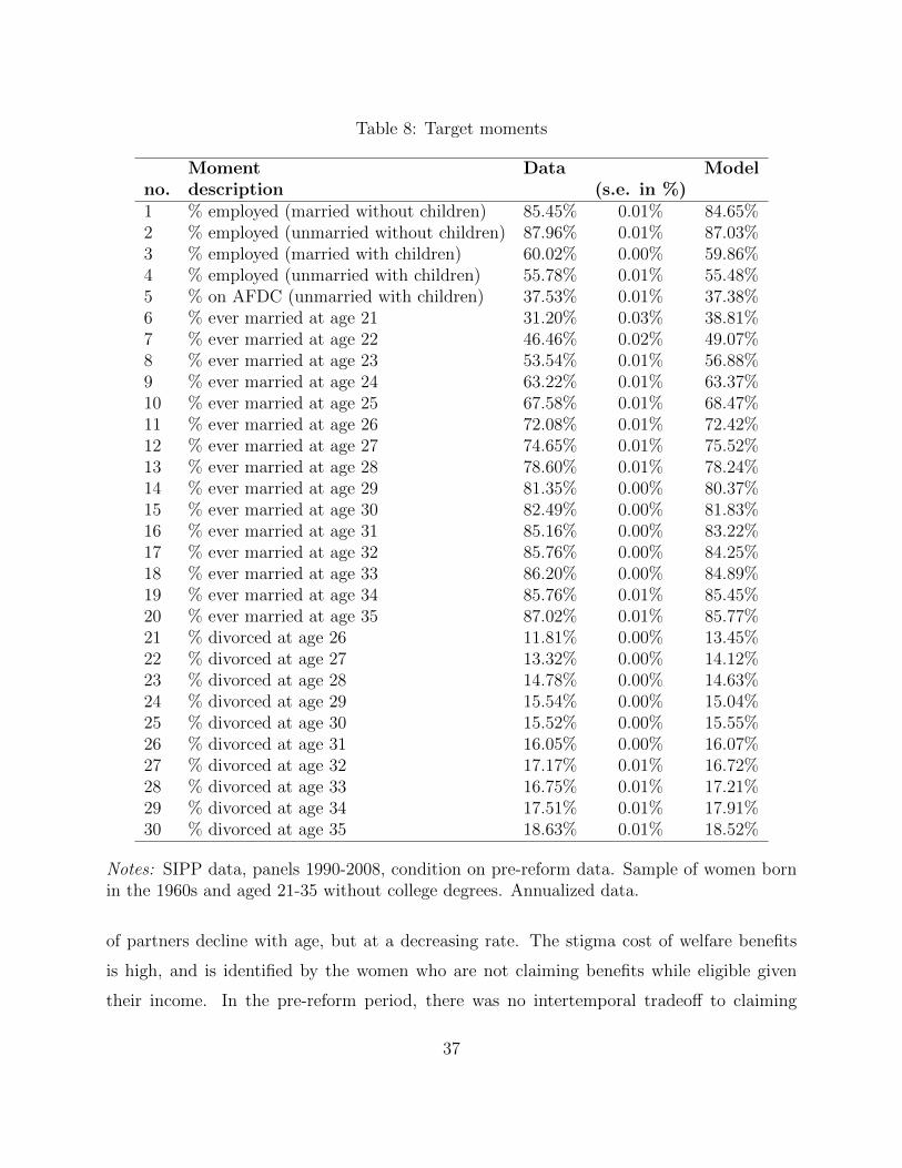
Table 8: Target moments

Moment Data Modelno. description (s.e. in %)1 % employed (married without children) 85.45% 0.01% 84.65%2 % employed (unmarried without children) 87.96% 0.01% 87.03%3 % employed (married with children) 60.02% 0.00% 59.86%4 % employed (unmarried with children) 55.78% 0.01% 55.48%5 % on AFDC (unmarried with children) 37.53% 0.01% 37.38%6 % ever married at age 21 31.20% 0.03% 38.81%7 % ever married at age 22 46.46% 0.02% 49.07%8 % ever married at age 23 53.54% 0.01% 56.88%9 % ever married at age 24 63.22% 0.01% 63.37%10 % ever married at age 25 67.58% 0.01% 68.47%11 % ever married at age 26 72.08% 0.01% 72.42%12 % ever married at age 27 74.65% 0.01% 75.52%13 % ever married at age 28 78.60% 0.01% 78.24%14 % ever married at age 29 81.35% 0.00% 80.37%15 % ever married at age 30 82.49% 0.00% 81.83%16 % ever married at age 31 85.16% 0.00% 83.22%17 % ever married at age 32 85.76% 0.00% 84.25%18 % ever married at age 33 86.20% 0.00% 84.89%19 % ever married at age 34 85.76% 0.01% 85.45%20 % ever married at age 35 87.02% 0.01% 85.77%21 % divorced at age 26 11.81% 0.00% 13.45%22 % divorced at age 27 13.32% 0.00% 14.12%23 % divorced at age 28 14.78% 0.00% 14.63%24 % divorced at age 29 15.54% 0.00% 15.04%25 % divorced at age 30 15.52% 0.00% 15.55%26 % divorced at age 31 16.05% 0.00% 16.07%27 % divorced at age 32 17.17% 0.01% 16.72%28 % divorced at age 33 16.75% 0.01% 17.21%29 % divorced at age 34 17.51% 0.01% 17.91%30 % divorced at age 35 18.63% 0.01% 18.52%

Notes: SIPP data, panels 1990-2008, condition on pre-reform data. Sample of women bornin the 1960s and aged 21-35 without college degrees. Annualized data.

of partners decline with age, but at a decreasing rate. The stigma cost of welfare benefits

is high, and is identified by the women who are not claiming benefits while eligible given

their income. In the pre-reform period, there was no intertemporal tradeoff to claiming

37

benefits, and hence we can attribute not claiming to utility or other costs of claiming. In the

counterfactual simulations, for the post reform period, the intertemporal tradeoff will add to

this cost, which makes it important to identify the utility cost from the pre-reform period.

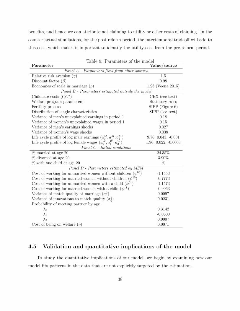
Table 9: Parameters of the modelParameter Value/source

Panel A - Parameters fixed from other sourcesRelative risk aversion (γ) 1.5Discount factor (β) 0.98Economies of scale in marriage (ρ) 1.23 (Voena 2015)

Panel B - Parameters estimated outside the modelChildcare costs (CCa) CEX (see text)Welfare program parameters Statutory rulesFertility process SIPP (Figure 6)Distribution of single characteristics SIPP (see text)Variance of men’s unexplained earnings in period 1 0.18Variance of women’s unexplained wages in period 1 0.15Variance of men’s earnings shocks 0.027Variance of women’s wage shocks 0.038Life cycle profile of log male earnings (aM0 , a

M1 , a

M2 ) 9.76, 0.043, -0.001

Life cycle profile of log female wages (aW0 , aW1 , a

W2 ) 1.96, 0.022, -0.0003

Panel C - Initial conditions% married at age 20 24.35%% divorced at age 20 3.90%% with one child at age 20 %

Panel D - Parameters estimated by MSMCost of working for unmarried women without children (ψ00) -1.1453Cost of working for married women without children (ψ10) -0.7773Cost of working for unmarried women with a child (ψ01) -1.1573Cost of working for married women with a child (ψ11) -0.9963Variance of match quality at marriage (σ2

0) 0.0097Variance of innovations to match quality (σ2

ξ ) 0.0231Probability of meeting partner by age

λ0 0.3142λ1 -0.0300λ2 0.0007

Cost of being on welfare (η) 0.0071

4.5 Validation and quantitative implications of the model

To study the quantitative implications of our model, we begin by examining how our

model fits patterns in the data that are not explicitly targeted by the estimation.

38

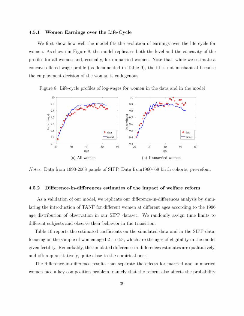
4.5.1 Women Earnings over the Life-Cycle

We first show how well the model fits the evolution of earnings over the life cycle for

women. As shown in Figure 8, the model replicates both the level and the concavity of the

profiles for all women and, crucially, for unmarried women. Note that, while we estimate a

concave offered wage profile (as documented in Table 9), the fit is not mechanical because

the employment decision of the woman is endogenous.

Figure 8: Life-cycle profiles of log-wages for women in the data and in the model

20 30 40 50 60age

9.3

9.4

9.5

9.6

9.7

9.8

9.9

10

ln(earnings)

datamodel

(a) All women

20 30 40 50 60age

9.3

9.4

9.5

9.6

9.7

9.8

9.9

10

ln(earnings)

datamodel

(b) Unmarried women

Notes: Data from 1990-2008 panels of SIPP. Data from1960-’69 birth cohorts, pre-refom.

4.5.2 Difference-in-differences estimates of the impact of welfare reform

As a validation of our model, we replicate our difference-in-differences analysis by simu-

lating the introduction of TANF for different women at different ages according to the 1996

age distribution of observation in our SIPP dataset. We randomly assign time limits to

different subjects and observe their behavior in the transition.

Table 10 reports the estimated coefficients on the simulated data and in the SIPP data,

focusing on the sample of women aged 21 to 53, which are the ages of eligibility in the model

given fertility. Remarkably, the simulated difference-in-differences estimates are qualitatively,

and often quantitatively, quite close to the empirical ones.

The difference-in-difference results that separate the effects for married and unmarried

women face a key composition problem, namely that the reform also affects the probability

39

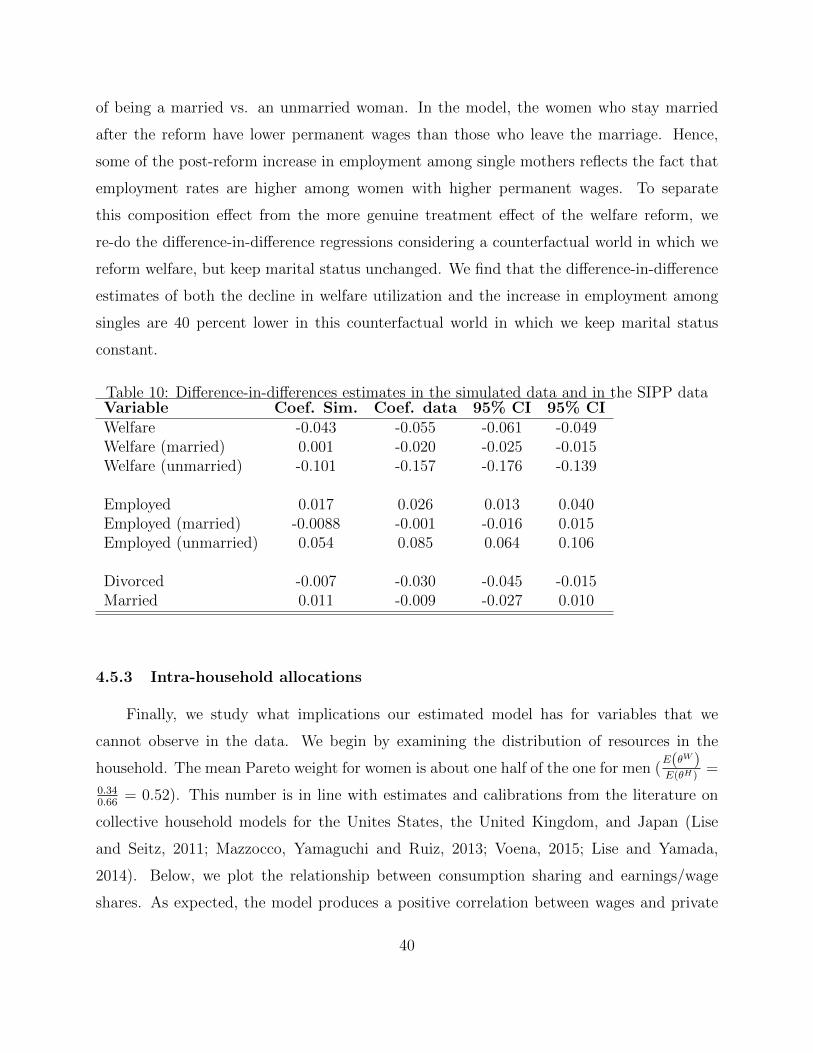
of being a married vs. an unmarried woman. In the model, the women who stay married

after the reform have lower permanent wages than those who leave the marriage. Hence,

some of the post-reform increase in employment among single mothers reflects the fact that

employment rates are higher among women with higher permanent wages. To separate

this composition effect from the more genuine treatment effect of the welfare reform, we

re-do the difference-in-difference regressions considering a counterfactual world in which we

reform welfare, but keep marital status unchanged. We find that the difference-in-difference

estimates of both the decline in welfare utilization and the increase in employment among

singles are 40 percent lower in this counterfactual world in which we keep marital status

constant.

Table 10: Difference-in-differences estimates in the simulated data and in the SIPP dataVariable Coef. Sim. Coef. data 95% CI 95% CIWelfare -0.043 -0.055 -0.061 -0.049Welfare (married) 0.001 -0.020 -0.025 -0.015Welfare (unmarried) -0.101 -0.157 -0.176 -0.139

Employed 0.017 0.026 0.013 0.040Employed (married) -0.0088 -0.001 -0.016 0.015Employed (unmarried) 0.054 0.085 0.064 0.106

Divorced -0.007 -0.030 -0.045 -0.015Married 0.011 -0.009 -0.027 0.010

4.5.3 Intra-household allocations

Finally, we study what implications our estimated model has for variables that we

cannot observe in the data. We begin by examining the distribution of resources in the

household. The mean Pareto weight for women is about one half of the one for men (E(θW )E(θH)

=

0.340.66

= 0.52). This number is in line with estimates and calibrations from the literature on

collective household models for the Unites States, the United Kingdom, and Japan (Lise

and Seitz, 2011; Mazzocco, Yamaguchi and Ruiz, 2013; Voena, 2015; Lise and Yamada,

2014). Below, we plot the relationship between consumption sharing and earnings/wage

shares. As expected, the model produces a positive correlation between wages and private

40

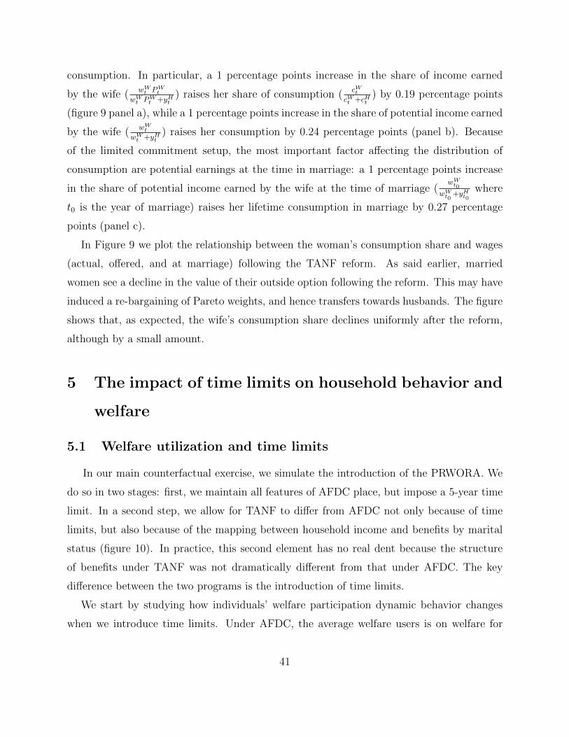
consumption. In particular, a 1 percentage points increase in the share of income earned

by the wife (wWt PWt

wWt PWt +yHt) raises her share of consumption (

cWtcWt +cHt

) by 0.19 percentage points

(figure 9 panel a), while a 1 percentage points increase in the share of potential income earned

by the wife (wWt

wWt +yHt) raises her consumption by 0.24 percentage points (panel b). Because

of the limited commitment setup, the most important factor affecting the distribution of

consumption are potential earnings at the time in marriage: a 1 percentage points increase

in the share of potential income earned by the wife at the time of marriage (wWt0

wWt0+yHt0

where

t0 is the year of marriage) raises her lifetime consumption in marriage by 0.27 percentage

points (panel c).

In Figure 9 we plot the relationship between the woman’s consumption share and wages

(actual, offered, and at marriage) following the TANF reform. As said earlier, married

women see a decline in the value of their outside option following the reform. This may have

induced a re-bargaining of Pareto weights, and hence transfers towards husbands. The figure

shows that, as expected, the wife’s consumption share declines uniformly after the reform,

although by a small amount.

5 The impact of time limits on household behavior and

welfare

5.1 Welfare utilization and time limits

In our main counterfactual exercise, we simulate the introduction of the PRWORA. We

do so in two stages: first, we maintain all features of AFDC place, but impose a 5-year time

limit. In a second step, we allow for TANF to differ from AFDC not only because of time

limits, but also because of the mapping between household income and benefits by marital

status (figure 10). In practice, this second element has no real dent because the structure

of benefits under TANF was not dramatically different from that under AFDC. The key

difference between the two programs is the introduction of time limits.

We start by studying how individuals’ welfare participation dynamic behavior changes

when we introduce time limits. Under AFDC, the average welfare users is on welfare for

41

Figure 9: Consumption allocation in the household

0 0.2 0.4 0.6 0.8 1wife's share of earnings

0.3

0.35

0.4

0.45

0.5

0.55

0.6w

ife's

shar

e of

con

sum

ptio

n

AFDCAFDC + time limit

(a) Earnings

0 0.2 0.4 0.6 0.8 1wife's share of potential earnings

0.3

0.35

0.4

0.45

0.5

0.55

0.6

wife

's sh

are

of c

onsu

mpt

ion

AFDCAFDC + time limit

(b) Offer wages

0 0.2 0.4 0.6 0.8 1wife's share of potential earnings at marriage

0.3

0.35

0.4

0.45

0.5

0.55

0.6

wife

's sh

are

of c

onsu

mpt

ion

AFDCAFDC + time limit

(c) Offer wages at marriage

6.12 years. Time limits, once introduced, are binding for 11.8% of women under AFDC, and

we observe significant bunching at 5 years once the limit is introduced (figure 11). Under

a 5-year time limit, the average utilization among welfare users drops to 3.34 years, and to

3.17 years under TANF. There is substantial bunching at 5 years, but also a reduction in

overall utilization, due to banking (figure 11). This is visible in the increased fraction of

people who are never taking up benefits under TANF. In a model with myopic behavior, of

course, the distribution under TANF would look identical to the one under AFDC with the

exception of the mass at 6+ moving to the 5-year support corner.

42

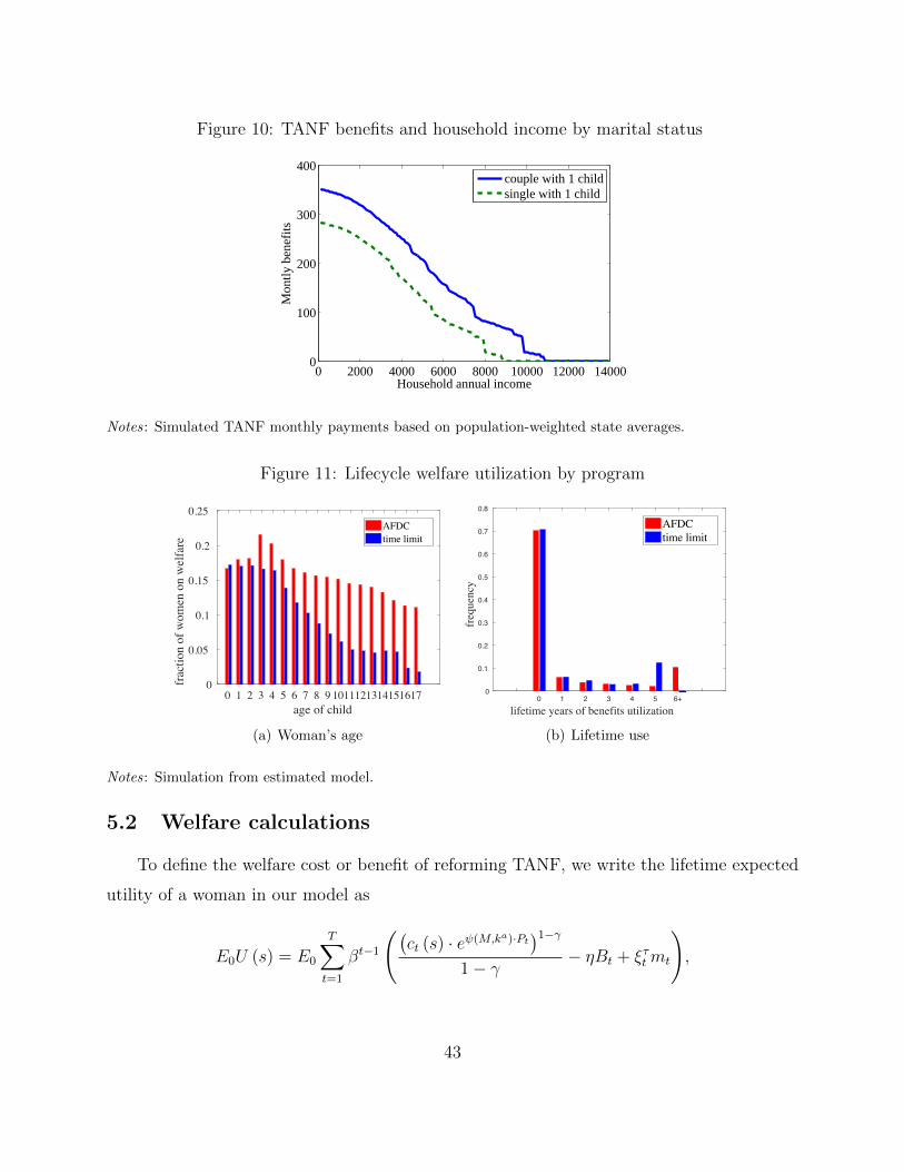
Figure 10: TANF benefits and household income by marital status

0 2000 4000 6000 8000 10000 12000 140000

100

200

300

400

Household annual income

Mon

tly b

enef

its

couple with 1 childsingle with 1 child

Notes: Simulated TANF monthly payments based on population-weighted state averages.

Figure 11: Lifecycle welfare utilization by program

0 1 2 3 4 5 6 7 8 9 1011121314151617age of child

0

0.05

0.1

0.15

0.2

0.25

fract

ion

of w

omen

on

wel

fare

AFDCtime limit

(a) Woman’s age

0 1 2 3 4 5 6+

lifetime years of benefits utilization

0

0.1

0.2

0.3

0.4

0.5

0.6

0.7

0.8

frequ

ency

AFDCtime limit

(b) Lifetime use

Notes: Simulation from estimated model.

5.2 Welfare calculations

To define the welfare cost or benefit of reforming TANF, we write the lifetime expected

utility of a woman in our model as

E0U (s) = E0

T∑t=1

βt−1

((ct (s) · eψ(M,ka)·Pt

)1−γ1− γ

− ηBt + ξτtmt

),

43

Figure 12: Fraction of household who reach the 5-year benefits utilization levels by age ofthe youngest child

0 1 2 3 4 5 6 7 8 9 1011121314151617age of child

0

0.05

0.1

0.15

0.2

0.25

fract

ion

with

5+

year

s use

d

AFDCtime limit

where ct, Pt, Bt,mt refer to the implied consumption, labor supply, benefit stream and

marital status in the baseline economy (s = AFDC) or in an alternative economy with

different welfare parameters (e.g. (s = TANF )). E0 represents the expectation at the

beginning of working life (before period 1).

When performing the policy experiments ,we use as a baseline a case in which the payroll

tax rate on labor is set to 0, and hence we let the government run a deficit D. When

varying parameters from AFDC to TANF (changes in benefits and time limits), we hold

the government budget deficit D constant. This is achieved by adjusting the proportional

payroll tax, τw, such that the present discounted value of net revenue flows remains constant:

N∑i=1

T∑t=1

1

(1 + r)t−1[FSit + EITCit + bit] =

N∑i=1

T∑t=1

1

(1 + r)t−1τwwitPit + D

where b captures the payment through AFDC or TANF. This calculation can be carried

out using realized payments.20

20Note that the summation is across individuals, i, who are the women. This is because our simulationsdo not keep track of men unless they are in a relationship. So, benefits are being spent on the women andthe extra tax to cover that is being taken from the women. Hence, the amount of taxes raised from the menis held constant and budget balance comes only from women.

44

In practice, we first calculate the left hand side in the baseline. This gives the size of

D = 172 per capita when τ = 0. Second, we change the policy rule into TANF and recalculate

the LHS. This gives the new deficit if the tax rate remains at zero (D′ = 73 per capita).

Third, we iterate on τ so that the deficit under the new policy is equal to D. As τ adjusts,

the choices individuals make will change and so the model needs to be resolved. However,

the final iteration gives the behavior of individuals in the new policy regime holding revenue

constant.

What we are asking is what proportion of consumption an individual is willing to pay

ex-ante to be indifferent between environment s′ = TANF and s = AFDC. Note that ex-

ante, no one knows the resulting sequence and since there are no aggregate shocks, realized

discounted lifetime utility averaged across all individuals will be equal to expected utility.

E0U (TANF, τw) |π =N∑i=1

T∑t=0

βt

(((1− π) c (TANF ) · eψ(M,ka)·P )1−γ

1− γ− ηBt

)(5)

We solve for π such that

E0U (TANF, τw) |π= E0U (b) , (6)

where π can be interpreted as the consumption cost of going from AFDC to TANF.

The results suggest that women are willing to pay 0.46% of lifetime consumption to be

indifferent between the new program (TANF) and the old version of it (AFDC). For single

mothers, for whom welfare benefits are more valuable, the willingness to pay is higher (2%

of lifetime consumption). This is an important calculation because it shows that - ”beyond

the veil of ignorance” - the 1996 reform, while achieving its main goals of breaking the

culture of welfare dependence and emphasizing one of self-sufficiency through work, induced

a net welfare loss by reducing insurance available to low-income women without reducing

the risks they face in the labor and marriage markets. Of course, this conclusion ignores

that the exercise is conducted by considering a balanced budget that involves only women

contribution, i.e., ignores possible corss-subsidization taking place across gender.

In our last exercise, reported in Table 11, we analyze the long-term consequences of the

45

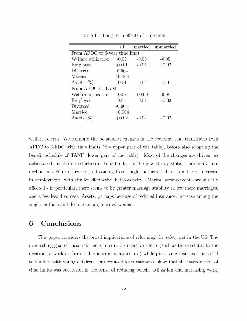
Table 11: Long-term effects of time limit

all married unmarriedFrom AFDC to 5-year time limitWelfare utilization -0.02 -0.00 -0.05Employed +0.01 -0.01 +0.02Divorced -0.004Married +0.004Assets (%) -0.01 -0.04 +0.01From AFDC to TANFWelfare utilization -0.03 +0.00 -0.05Employed 0.01 -0.01 +0.03Divorced -0.004Married +0.004Assets (%) +0.02 -0.02 +0.02

welfare reform. We compute the behavioral changes in the economy that transitions from

AFDC to AFDC with time limits (the upper part of the table), before also adopting the

benefit schedule of TANF (lower part of the table). Most of the changes are driven, as

anticipated, by the introduction of time limits. In the new steady state, there is a 3 p.p.

decline in welfare utilization, all coming from single mothers. There is a 1 p.p. increase

in employment, with similar distinctive heterogeneity. Marital arrangements are slightly

affected - in particular, there seems to be greater marriage stability (a few more marriages,

and a few less divorces). Assets, perhaps because of reduced insurance, increase among the

single mothers and decline among married women.

6 Conclusions

This paper considers the broad implications of reforming the safety net in the US. The

overarching goal of these reforms is to curb disincentive effects (such as those related to the

decision to work or form stable marital relationships) while preserving insurance provided

to families with young children. Our reduced form estimates show that the introduction of

time limits was successful in the sense of reducing benefit utilization and increasing work,

46

with the effects mostly concentrated among single mothers (who were the largest group of

beneficiaries in the pre-reform period). Moreover, the reform seems to have reduced divorce

rates (with insignificant effects on marriage rates or fertility). Our life-cycle model with

endogenous marriage replicates these outcomes. In particular, forward-looking behavior is

evident in the banking of TANF benefits. For most women, the time limit is not reached

because of the option value of waiting for periods when benefits have most value (such as

periods of low offered wages). We find that changes in marital status are an important part

of the adjustment process following the reform. Welfare analyses reveal that the groups

mostly targeted by the reform (i.e., single mothers) suffered a net welfare loss, despite the

increase in self-sufficiency brought about by increasing employment.

47

References

Attanasio, O., H. Low, and V. Sanchez-Marcos. 2008. “Explaining changes in femalelabor supply in a life-cycle model.” The American Economic Review, 98(4): 1517–1552.

Bitler, Marianne P, Jonah B Gelbach, Hilary W Hoynes, and Madeline Zavodny.2004. “The impact of welfare reform on marriage and divorce.” Demography, 41(2): 213–236.

Blank, Rebecca M. 2002. “Evaluating Welfare Reform in the United States.” Journal ofEconomic Literature, 40(4): 1105–1166.

Blundell, Richard, Alan Duncan, and Costas Meghir. 1998. “Estimating labor supplyresponses using tax reforms.” Econometrica, 827–861.

Blundell, Richard, Monica Costa Dias, Costas Meghir, and Jonathan M Shaw.2016. “Female labour supply, human capital and welfare reform.”

Blundell, Richard, Pierre-Andre Chiappori, and Costas Meghir. 2005. “Collectivelabor supply with children.” Journal of political Economy, 113(6): 1277–1306.

Bronson, Mary Ann. 2014. “Degrees are forever: Marriage, educational investment, andlifecycle labor decisions of men and women.” Unpublished manuscript, 2.

Burtless, Gary, and Jerry A Hausman. 1978. “The effect of taxation on labor supply:Evaluating the Gary negative income tax experiment.” The Journal of Political Economy,1103–1130.

Chan, Marc K. 2013. “A Dynamic Model of Welfare Reform.” Econometrica, 81(3): 941–1001.

Chiappori, Pierre-Andre. 1988. “Rational household labor supply.” Econometrica: Jour-nal of the Econometric Society, 63–90.

Chiappori, Pierre-Andre. 1992. “Collective labor supply and welfare.” Journal of politicalEconomy, 437–467.

Eissa, Nada, and Jeffrey B Liebman. 1995. “Labor supply response to the earned incometax credit.” National Bureau of Economic Research.

Fernandez, Raquel, and Joyce Cheng Wong. 2014. “Divorce Risk, Wages and WorkingWives: A Quantitative Life-Cycle Analysis of Female Labour Force Participation.” TheEconomic Journal, 124(576): 319–358.

Grogger, Jeffrey, and Charles Michalopoulos. 2003. “Welfare Dynamics under TimeLimits.” Journal of Political Economy, 111(3).

48

Grogger, Jeffrey, and Lynn A. Karoly. 2005. Welfare Reform. Harvard University Press.

Heckman, James. 1974. “Shadow prices, market wages, and labor supply.” Econometrica:journal of the econometric society, 679–694.

Kaplan, Greg. 2012. “Moving back home: Insurance against labor market risk.” Journalof Political Economy, 120(3): 446–512.

Keane, Michael, and Robert Moffitt. 1998. “A structural model of multiple welfareprogram participation and labor supply.” International economic review, 553–589.

Keane, Michael P, and Kenneth I Wolpin. 1997. “The career decisions of young men.”Journal of political Economy, 105(3): 473–522.

Keane, Michael P, and Kenneth I Wolpin. 2010. “The Role of Labor and MarriageMarkets, Preference Heterogeneity, and the Welfare System in the Life Cycle Decisions ofBlack, Hispanic, and White Women*.” International Economic Review, 51(3): 851–892.

Kline, Patrick, and Melissa Tartari. forthcoming. “Bounding the Labor Supply Re-sponses to a Randomized Welfare Experiment: A Revealed Preference Approach.” TheAmerican Economic Review.

Kocherlakota, N.R. 1996. “Implications of efficient risk sharing without commitment.”The Review of Economic Studies, 63(4): 595–609.

Ligon, E., J.P. Thomas, and T. Worrall. 2002a. “Informal insurance arrangementswith limited commitment: Theory and evidence from village economies.” The Review ofEconomic Studies, 69(1): 209–244.

Ligon, Ethan, Jonathan P Thomas, and Tim Worrall. 2000. “Mutual insurance,individual savings, and limited commitment.” Review of Economic Dynamics, 3(2): 216–246.

Ligon, Ethan, Jonathan P Thomas, and Tim Worrall. 2002b. “Informal insurancearrangements with limited commitment: Theory and evidence from village economies.”The Review of Economic Studies, 69(1): 209–244.

Lise, Jeremy, and Ken Yamada. 2014. “Household sharing and commitment: Evidencefrom panel data on individual expenditures and time use.” IFS Working Papers.

Lise, Jeremy, and Shannon Seitz. 2011. “Consumption inequality and intra-householdallocations.” The Review of Economic Studies, 78(1): 328–355.

Low, Hamish, and Luigi Pistaferri. 2015. “Disability risk, disability insurance and lifecycle behavior.” American Economic Review, 105(10): 2986–3029.

49

Mazzocco, M. 2007a. “Household intertemporal behaviour: A collective characterizationand a test of commitment.” Review of Economic Studies, 74(3): 857–895.

Mazzocco, Maurizio. 2007b. “Household intertemporal behaviour: A collective character-ization and a test of commitment.” The Review of Economic Studies, 74(3): 857–895.

Mazzocco, M., S. Yamaguchi, and C. Ruiz. 2013. “Labor supply, wealth dynamics,and marriage decisions.”

Mazzolari, Francesca, and Giuseppe Ragusa. 2012. “Time Limits: The Effects on Wel-fare Use and Other Consumption-Smoothing Mechanisms.” IZA discussion paper No.6993.

McFadden, Daniel. 1989. “A method of simulated moments for estimation of discrete re-sponse models without numerical integration.” Econometrica: Journal of the EconometricSociety, 995–1026.

Pakes, Ariel, and David Pollard. 1989. “Simulation and the Asymptotics of OptimizationEstimators.” Econometrica, 57(5): 1027–1057.

Persson, Petra. 2014. “Social insurance and the marriage market.” Unpublishedmanuscript.

Rothstein, Jesse. 2010. “Is the EITC as Good as an NIT? Conditional Cash Transfers andTax Incidence.” American Economic Journal: Economic Policy, 2(1): 177–208.

Swann, Christopher A. 2005. “Welfare reform when recipients are forward-looking.” Jour-nal of Human Resources, 40(1): 31–56.

Voena, Alessandra. 2015. “Yours, Mine and Ours: Do Divorce Laws Affect the Intertem-poral Behavior of Married Couples?” American Economic Review, forthcoming.

Zabel, Jeffrey E. 1998. “An analysis of attrition in the Panel Study of Income Dynamicsand the Survey of Income and Program Participation with an application to a model oflabor market behavior.” Journal of Human Resources, 479–506.

50

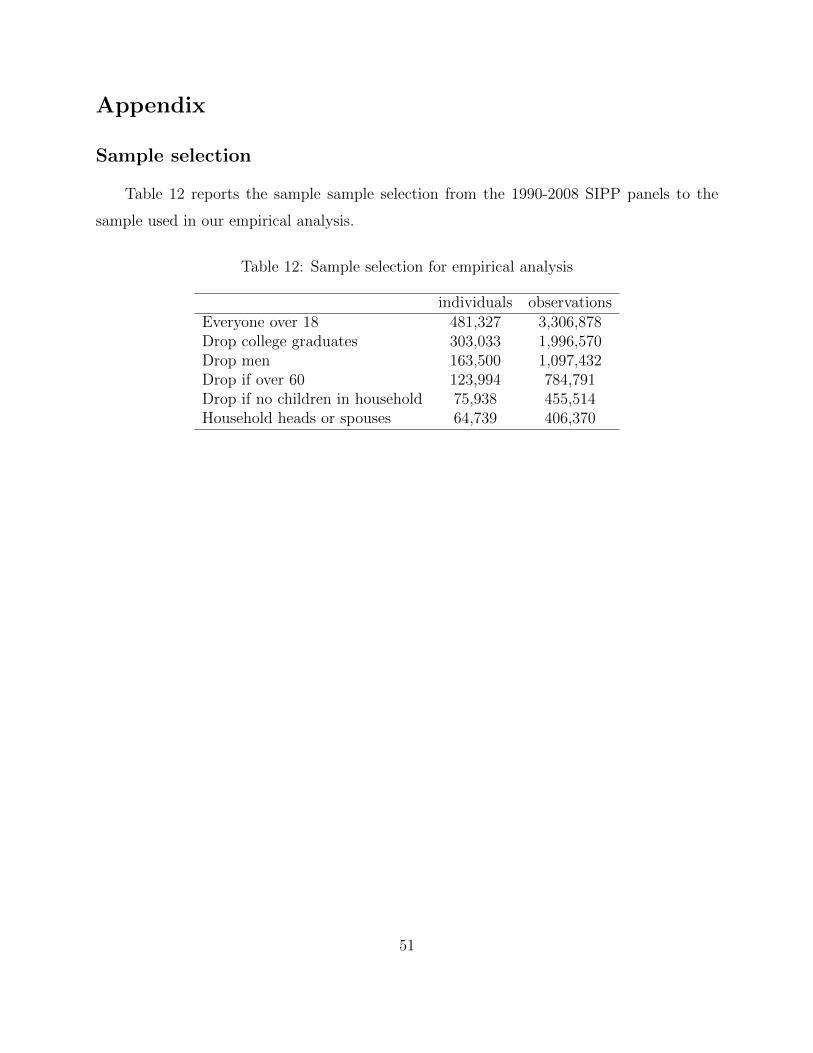
Appendix

Sample selection

Table 12 reports the sample sample selection from the 1990-2008 SIPP panels to the

sample used in our empirical analysis.

Table 12: Sample selection for empirical analysis

individuals observationsEveryone over 18 481,327 3,306,878Drop college graduates 303,033 1,996,570Drop men 163,500 1,097,432Drop if over 60 123,994 784,791Drop if no children in household 75,938 455,514Household heads or spouses 64,739 406,370

51

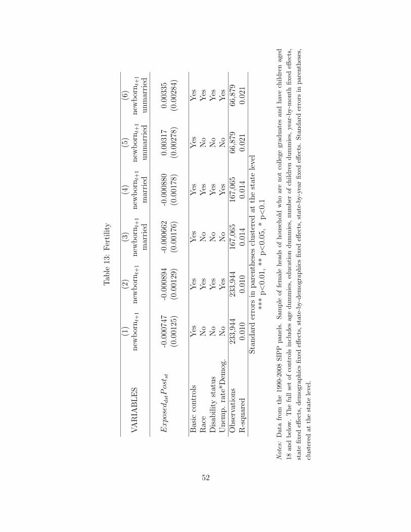
Tab

le13

:F

erti

lity

(1)

(2)

(3)

(4)

(5)

(6)

VA

RIA

BL

ES

new

bor

nt+

1new

bor

nt+

1new

bor

nt+

1new

bor

nt+

1new

bor

nt+

1new

bor

nt+

1

mar

ried

mar

ried

unm

arri

edunm

arri

ed

ExposeddstPost st

-0.0

0074

7-0

.000

894

-0.0

0066

2-0

.000

880

0.00

317

0.00

335

(0.0

0125

)(0

.001

29)

(0.0

0176

)(0

.001

78)

(0.0

0278

)(0

.002

84)

Bas

icco

ntr

ols

Yes

Yes

Yes

Yes

Yes

Yes

Rac

eN

oY

esN

oY

esN

oY

esD

isab

ilit

yst

atus

No

Yes

No

Yes

No

Yes

Unem

p.

rate

*Dem

og.

No

Yes

No

Yes

No

Yes

Obse

rvat

ions

233,

944

233,

944

167,

065

167,

065

66,8

7966

,879

R-s

quar

ed0.

010

0.01

00.

014

0.01

40.

021

0.02

1Sta

ndar

der

rors

inpar

enth

eses

clust

ered

atth

est

ate

leve

l**

*p<

0.01

,**

p<

0.05

,*

p<

0.1

Notes:

Dat

afr

omth

e19

90-2

008

SIP

Ppanel

s.S

am

ple

of

fem

ale

hea

ds

of

hou

seh

old

wh

oare

not

coll

ege

gra

du

ate

san

dh

ave

chil

dre

naged

18an

db

elow

.T

he

full

set

ofco

ntr

ols

incl

ud

esage

du

mm

ies,

edu

cati

on

du

mm

ies,

nu

mb

erof

chil

dre

nd

um

mie

s,ye

ar-

by-m

onth

fixed

effec

ts,

stat

efi

xed

effec

ts,

dem

ogra

ph

ics

fixed

effec

ts,

state

-by-d

emogra

ph

ics

fixed

effec

ts,

state

-by-y

ear

fixed

effec

ts.

Sta

nd

ard

erro

rsin

pare

nth

eses

,

clu

ster

edat

the

stat

ele

vel

.

52

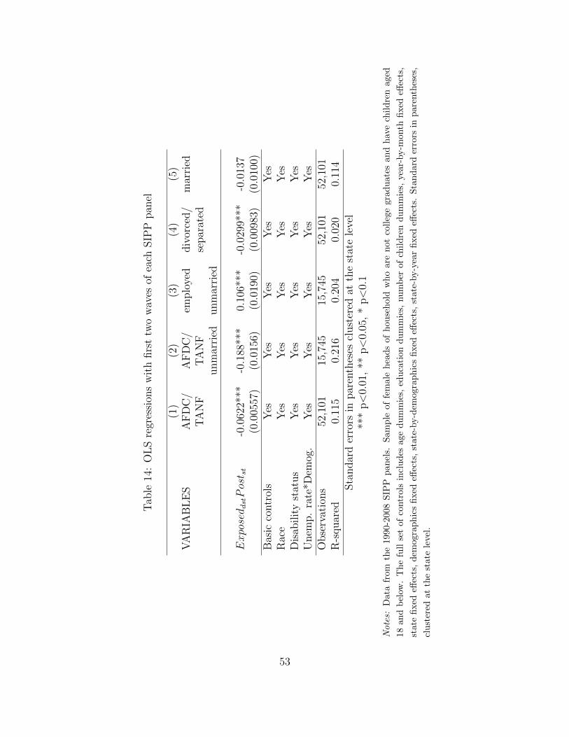
Tab

le14

:O

LS

regr

essi

ons

wit

hfirs

ttw

ow

aves

ofea

chSIP

Ppan

el

(1)

(2)

(3)

(4)

(5)

VA

RIA

BL

ES

AF

DC

/A

FD

C/

emplo

yed

div

orce

d/

mar

ried

TA

NF

TA

NF

separ

ated

unm

arri

edunm

arri

ed

ExposeddstPost st

-0.0

622*

**-0

.188

***

0.10

6***

-0.0

299*

**-0

.013

7(0

.005

57)

(0.0

156)

(0.0

190)

(0.0

0983

)(0

.010

0)B

asic

contr

ols

Yes

Yes

Yes

Yes

Yes

Rac

eY

esY

esY

esY

esY

esD

isab

ilit

yst

atus

Yes

Yes

Yes

Yes

Yes

Unem

p.

rate

*Dem

og.

Yes

Yes

Yes

Yes

Yes

Obse

rvat

ions

52,1

0115

,745

15,7

4552

,101

52,1

01R

-squar

ed0.

115

0.21

60.

204

0.02

00.

114

Sta

ndar

der

rors

inpar

enth

eses

clust

ered

atth

est

ate

leve

l**

*p<

0.01

,**

p<

0.05

,*

p<

0.1

Notes:

Dat

afr

omth

e19

90-2

008

SIP

Ppanel

s.S

am

ple

of

fem

ale

hea

ds

of

hou

seh

old

wh

oare

not

coll

ege

gra

du

ate

san

dh

ave

chil

dre

naged

18an

db

elow

.T

he

full

set

ofco

ntr

ols

incl

ud

esage

du

mm

ies,

edu

cati

on

du

mm

ies,

nu

mb

erof

chil

dre

nd

um

mie

s,ye

ar-

by-m

onth

fixed

effec

ts,

stat

efi

xed

effec

ts,

dem

ogra

ph

ics

fixed

effec

ts,

state

-by-d

emogra

ph

ics

fixed

effec

ts,

state

-by-y

ear

fixed

effec

ts.

Sta

nd

ard

erro

rsin

pare

nth

eses

,

clu

ster

edat

the

stat

ele

vel

.

53

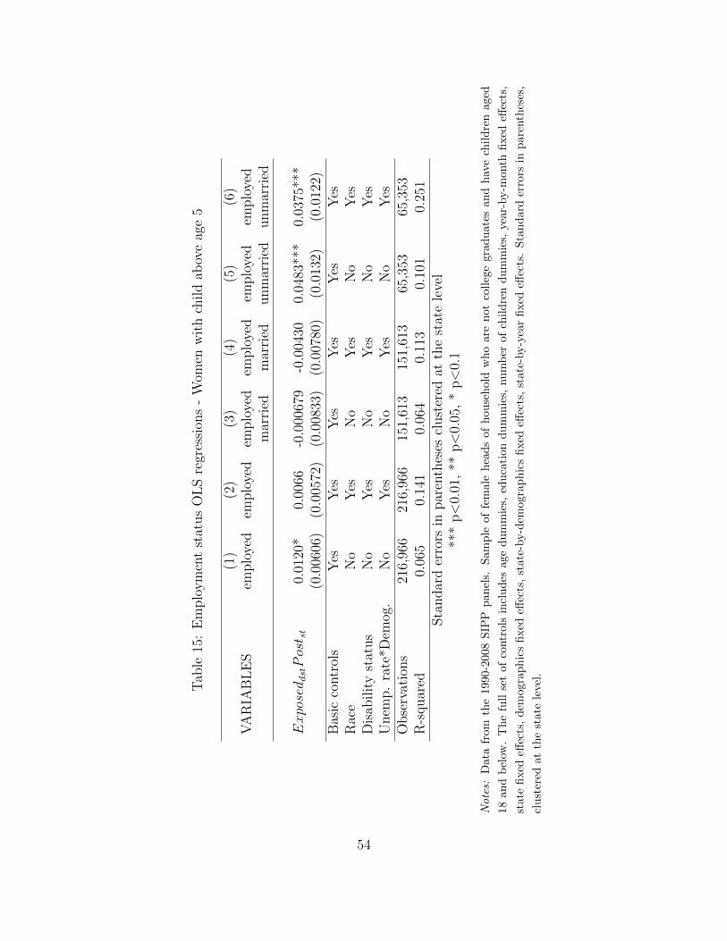
Tab

le15

:E

mplo

ym

ent

stat

us

OL

Sre

gres

sion

s-

Wom

enw

ith

child

abov

eag

e5

(1)

(2)

(3)

(4)

(5)

(6)

VA

RIA

BL

ES

emplo

yed

emplo

yed

emplo

yed

emplo

yed

emplo

yed

emplo

yed

mar

ried

mar

ried

unm

arri

edunm

arri

ed

ExposeddstPost st

0.01

20*

0.00

66-0

.000

679

-0.0

0430

0.04

83**

*0.

0375

***

(0.0

0606

)(0

.005

72)

(0.0

0833

)(0

.007

80)

(0.0

132)

(0.0

122)

Bas

icco

ntr

ols

Yes

Yes

Yes

Yes

Yes

Yes

Rac

eN

oY

esN

oY

esN

oY

esD

isab

ilit

yst

atus

No

Yes

No

Yes

No

Yes

Unem

p.

rate

*Dem

og.

No

Yes

No

Yes

No

Yes

Obse

rvat

ions

216,

966

216,

966

151,

613

151,

613

65,3

5365

,353

R-s

quar

ed0.

065

0.14

10.

064

0.11

30.

101

0.25

1Sta

ndar

der

rors

inpar

enth

eses

clust

ered

atth

est

ate

leve

l**

*p<

0.01

,**

p<

0.05

,*

p<

0.1

Notes:

Dat

afr

omth

e19

90-2

008

SIP

Ppanel

s.S

am

ple

of

fem

ale

hea

ds

of

hou

seh

old

wh

oare

not

coll

ege

gra

du

ate

san

dh

ave

chil

dre

naged

18an

db

elow

.T

he

full

set

ofco

ntr

ols

incl

ud

esage

du

mm

ies,

edu

cati

on

du

mm

ies,

nu

mb

erof

chil

dre

nd

um

mie

s,ye

ar-

by-m

onth

fixed

effec

ts,

stat

efi

xed

effec

ts,

dem

ogra

ph

ics

fixed

effec

ts,

state

-by-d

emogra

ph

ics

fixed

effec

ts,

state

-by-y

ear

fixed

effec

ts.

Sta

nd

ard

erro

rsin

pare

nth

eses

,

clu

ster

edat

the

stat

ele

vel

.

54

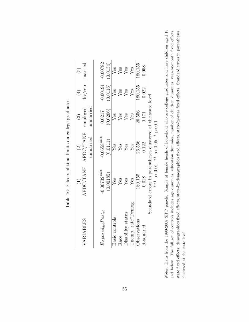
Tab

le16

:E

ffec

tsof

tim

elim

its

onco

lleg

egr

aduat

es

(1)

(2)

(3)

(4)

(5)

VA

RIA

BL

ES

AF

DC

/TA

NF

AF

DC

/TA

NF

emplo

yed

div

/sep

mar

ried

unm

arri

edunm

arri

ed

ExposeddstPost st

-0.0

0732

***

-0.0

658*

**0.

0217

-0.0

0191

-0.0

0782

(0.0

0185

)(0

.011

1)(0

.020

6)(0

.011

6)(0

.013

4)B

asic

contr

ols

Yes

Yes

Yes

Yes

Yes

Rac

eY

esY

esY

esY

esY

esD

isab

ilit

yst

atus

Yes

Yes

Yes

Yes

Yes

Unem

p.

rate

*Dem

og.

Yes

Yes

Yes

Yes

Yes

Obse

rvat

ions

180,

155

26,5

5626

,556

180,

155

180,

155

R-s

quar

ed0.

028

0.12

20.

171

0.02

20.

058

Sta

ndar

der

rors

inpar

enth

eses

clust

ered

atth

est

ate

leve

l**

*p<

0.01

,**

p<

0.05

,*

p<

0.1

Notes:

Dat

afr

omth

e19

90-2

008

SIP

Pp

anel

s.S

am

ple

of

fem

ale

hea

ds

of

house

hold

wh

oare

coll

ege

gra

duate

san

dh

ave

chil

dre

naged

18

and

bel

ow.

Th

efu

llse

tof

contr

ols

incl

ud

esag

ed

um

mie

s,ed

uca

tion

du

mm

ies,

nu

mb

erof

chil

dre

nd

um

mie

s,ye

ar-

by-m

onth

fixed

effec

ts,

stat

efi

xed

effec

ts,

dem

ogra

ph

ics

fixed

effec

ts,

state

-by-d

emogra

ph

ics

fixed

effec

ts,

state

-by-y

ear

fixed

effec

ts.

Sta

nd

ard

erro

rsin

pare

nth

eses

,

clu

ster

edat

the

stat

ele

vel

.

55

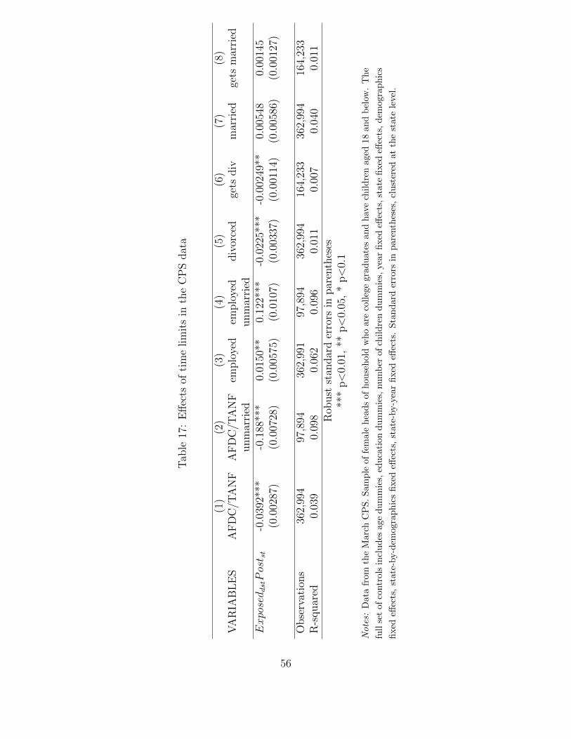
Tab

le17

:E

ffec

tsof

tim

elim

its

inth

eC

PS

dat

a

(1)

(2)

(3)

(4)

(5)

(6)

(7)

(8)

VA

RIA

BL

ES

AF

DC

/TA

NF

AF

DC

/TA

NF

emplo

yed

emplo

yed

div

orce

dge

tsdiv

mar

ried

gets

mar

ried

unm

arri

edunm

arri

edExposeddstPost st

-0.0

392*

**-0

.188

***

0.01

50**

0.12

2***

-0.0

225*

**-0

.002

49**

0.00

548

0.00

145

(0.0

0287

)(0

.007

28)

(0.0

0575

)(0

.010

7)(0

.003

37)

(0.0

0114

)(0

.005

86)

(0.0

0127

)

Obse

rvat

ions

362,

994

97,8

9436

2,99

197

,894

362,

994

164,

233

362,

994

164,

233

R-s

quar

ed0.

039

0.09

80.

062

0.09

60.

011

0.00

70.

040

0.01

1R

obust

stan

dar

der

rors

inpar

enth

eses

***

p<

0.01

,**

p<

0.05

,*

p<

0.1

Notes:

Dat

afr

omth

eM

arch

CP

S.

Sam

ple

offe

male

hea

ds

of

hou

seh

old

wh

oare

coll

ege

gra

du

ate

san

dh

ave

chil

dre

naged

18

an

db

elow

.T

he

full

set

ofco

ntr

ols

incl

ud

esag

ed

um

mie

s,ed

uca

tion

du

mm

ies,

nu

mb

erof

chil

dre

nd

um

mie

s,ye

ar

fixed

effec

ts,

state

fixed

effec

ts,

dem

ogra

ph

ics

fixed

effec

ts,

stat

e-by-d

emog

rap

hic

sfi

xed

effec

ts,

state

-by-y

ear

fixed

effec

ts.

Sta

nd

ard

erro

rsin

pare

nth

eses

,cl

ust

ered

at

the

state

leve

l.

56

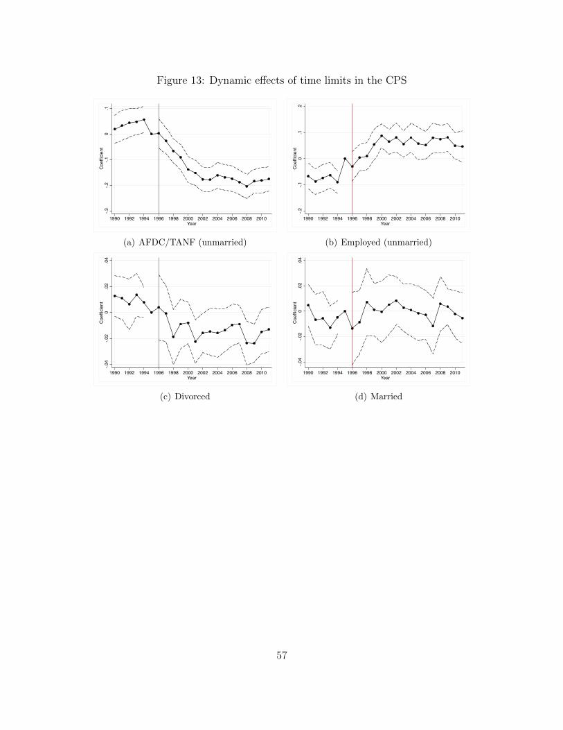
Figure 13: Dynamic effects of time limits in the CPS

-.3-.2

-.10

.1Coefficient

1990 1992 1994 1996 1998 2000 2002 2004 2006 2008 2010Year

(a) AFDC/TANF (unmarried)

-.2-.1

0.1

.2Coefficient

1990 1992 1994 1996 1998 2000 2002 2004 2006 2008 2010Year

(b) Employed (unmarried)

-.04

-.02

0.02

.04

Coefficient

1990 1992 1994 1996 1998 2000 2002 2004 2006 2008 2010Year

(c) Divorced

-.04

-.02

0.02

.04

Coefficient

1990 1992 1994 1996 1998 2000 2002 2004 2006 2008 2010Year

(d) Married

57