markov random field approach to region extraction using tabu search

www.elsevier.com/locate/jvci

J. Vis. Commun. Image R. 16 (2005) 134–158

Markov random field approachto region extraction using Tabu Search

Jose J. Amador*

National Aeronautics and Space Administration (NASA)/John F. Kennedy Space Center

KSC, FL 32899, USA

Received 10 December 2002; accepted 22 June 2004

Available online 23 August 2004

Abstract

This paper describes a region extraction algorithm based on the concept of Markov ran-

dom fields. Markov random fields (MRFs) are characterized by using a Gibbs Distribution

which equates back to the MRF. A heuristically developed energy functional is presented

and used with the MRF in an efficient and accurate manner. Since the MRF used in this work

is defined using the polar coordinate system, a very large search space exists for radial lengths

and sites. To aid in pursuing these radial sites, a combinatorial optimization technique known

as Tabu Search is exploited. Also provided is an extensive empirical study on aerial imagery

and parts detection, in addition to a final discussion and description of future work.

� 2004 Elsevier Inc. All rights reserved.

Keywords: Markov random field; Gibbs Distribution; Tabu Search; Region extraction

1. Introduction

Most computer vision research for approximately the past 30 years has focused

on low-level vision processes (Aksoy and Haralick, 1999; Ball and Hall, 1965; Cov-

er and Hart, 1967). Topics within this area include edge detection, region growing,

1047-3203/$ - see front matter � 2004 Elsevier Inc. All rights reserved.

doi:10.1016/j.jvcir.2004.06.002

* Fax: +1 321 867 3552.

E-mail address: [email protected].

mailto:[email protected].

J.J. Amador / J. Vis. Commun. Image R. 16 (2005) 134–158 135

and thresholding as primary methods (Duda and Hart, 1973; da Fortuna Costa and

Cesar, 2001). Only recently has some attention been given to further the knowledge

of intermediate-level vision processes (whose function performs exact region extrac-

tion of objects from images) primarily using low-level vision methods (Cramariuc et

al., 1997; Tomasi and Manduchi, 1998). These low-level vision techniques workwell if image properties are uniform or homogeneous (i.e., same gray-level, texture,

etc.). However, these methods are not applicable to regions whose image properties

are non-uniform or heterogeneous (e.g., a single object composed of various

materials or gray-levels). Therefore, what is needed is a new technique specific to

the intermediate-level vision goal that will extract regions of non-uniform image

properties.

Accordingly, the main focus of this paper is on region extraction. This paper pre-

sents an energy minimization technique that recognizes compact and closed objectscharacterized in polar coordinate form. A Markov random field (MRF) is then used

to represent and model these compact-closed objects which are subsequently incor-

porated into an energy minimization function. An initial high-level hypothesis is pro-

vided by a human, or image analyst; a combinatorial optimization technique known

as Tabu Search provides the means for driving the energy function to its global or

near-global optimum state. This paper will also show how the minimum energy state

corresponds to an MRF state of highest probability.

1.1. Prior work

To understand the uniqueness of this paper�s approach it becomes necessary to

review the results of related research. Of primary interest are disclosures which have

used an MRF methodology for region extraction (Delagnes and Barba, 1996; Gunsel

et al., 1994; Hill and Taylor, 1992; Li, 1994; Margalit and Rosenfeld, 1990; Modes-

tino and Zhang, 1992; Nadabar and Jain, 1996; Schluter et al., 2000). Several ap-

proaches have realized coupled MRFs (Gunsel et al., 1994; Li, 1994), novelextensions and techniques (Delagnes and Barba, 1996; Margalit and Rosenfeld,

1990; Schluter et al., 2000), and model-based MRFs (Hill and Taylor, 1992; Modes-

tino and Zhang, 1992; Nadabar and Jain, 1996).

For region extraction, MRFs have been developed under a coupled methodology

(Gunsel et al., 1994; Li, 1994). MRFs are coupled to each other via inter-relations,

such as distance between a point and a line constraining the two different features. In

Gunsel et al. (1994) boundary finding or edge detection is first performed followed

by a multiscale representation of coupled MRFs. This is then applied to a stochasticregularization scheme based on a Bayesian framework. Unfortunately, the method

requires choosing a pre-selected number of scales to be robust. The work of Li

(1994) presents a model to region extraction in support to a high-level vision process.

Region extraction is performed by using coupled MRFs within a Bayesian frame-

work. Results are defined as a maximum a posteriori estimate, instead of using a heu-

ristic technique. The results provide rotation- and scale-invariance, however,

extracted regions share common structures which cause significant ambiguities

requiring context (i.e., an analyst) to resolve.

136 J.J. Amador / J. Vis. Commun. Image R. 16 (2005) 134–158

The contribution of Margalit and Rosenfeld (1990) takes a probabilistic approach

to using MRFs reducing computational cost of template matching. In their work,

second-order gray-level probabilities of the image and template are gathered using

a base MRF method. These probabilities are used to compare matching pixels in

an efficient and appropriate order. Clearly, use of templates requires the creationof several templates at different rotations and scales. No quantitative or qualitative

discussion was provided describing how variations in rotation or scale are handled

other than using different templates.

Delagnes and Barba (1996) approached using MRFs for region extraction differ-

ently. MRFs are modeled for drawing out linear structures in poorly contrasted

images. Linear feature extraction is defined as an irregular lattice (i.e., an MRF),

subsequently, rectilinear patterns are accurately delineated from the lattice. This

method only works well for objects consisting merely of straight-line segments; thiswas shown experimentally for line detection on pavements.

The recent work of Schluter et al. (2000) approached region extraction using a

multi-layered MRF with contour-based grouping. Contour-based grouping is per-

formed at an intermediate level of vision processing; the MRF judge�s contours

based on hypotheses by applying geometrical constraints. Although the technique

worked well on analytical and arbitrarily shaped objects, all objects were of fixed size

and rotation. Furthermore, initial starting conditions are very sensitive, causing

expansion of the search space in some experiments and increasing the error rate.Another category in which MRFs support region extraction is model-based strat-

egies (Hill and Taylor, 1992; Modestino and Zhang, 1992; Nadabar and Jain, 1996).

These model-based methods, in general, develop a common representation for the

shape to detect. In all cases but one (Nadabar and Jain, 1996), the methods used

combinatorial optimization to find the best configuration of the model in image data

(Hill and Taylor, 1992; Modestino and Zhang, 1992). The scheme of Nadabar and

Jain (1996) estimates parameters of an MRF line process using geometrical com-

puter aided design (CAD) models of the object. Although MRF canonical represen-tation reduces the number of parameter estimates, region extraction occurs only by

creating a large database of objects. Modestino and Zhang (1992) segmented the im-

age into areas of homogeneous image properties where the areas form an adjacency

graph. Region extraction is modeled by an MRF on the graph whose best realization

is found by simulated annealing. Objects are interpreted by coarse contours (e.g.,

rectangular regions) delineating different areas. These regions only support a simplis-

tic understanding of the image, no detail is involved. The paper by Hill and Taylor

(1992) describes a model-based method using genetic algorithms. The genetic algo-rithm is used to search for MRF representations that best fit the model to the image.

The technique was designed for rotation- and scale-invariance, however, the model

was not designed to be arbitrary.

As described above, the MRF methodology for region extraction is effective in

most, but noticeably, not all cases. Different techniques exist to solve the region

extraction problem using MRFs with varied results. Although some results achieved

region extraction and rotation- or scale-invariance, none of the techniques were

able to solve all. The most recent work in the field offers an intermediate-level vision


process that effectively uses hypotheses. Nevertheless, the method was unable to deal

with heterogeneous regions (Schluter et al., 2000). Evidently, more improvements are

needed with MRF methodologies or another technique may be required.

1.2. Outline

Section 2 of this paper describes the MRF and Gibbs Distribution. Section 3 de-

scribes the energy functional used for this problem. Section 4 covers the optimization

technique, specifically, how Gibbs Distribution is used and an introduction to Tabu

Search. Furthermore, the region extraction algorithm is reviewed in detail. Section 5

then covers the empirical studies performed, and Section 6 provides concluding re-

marks and areas of future research.

2. Markov random field approach

In 1984, Geman and Geman (1984) wrote a seminal paper on an optimization

algorithm (i.e., simulated annealing) developed for restoring degraded images. Ge-

man and Geman showed that any energy functional satisfying simple conditions de-

fine a Gibbs Distribution over the sample space. One of their major contributions was

demonstrating a Gibbs Distribution as equivalent to the existence of an MRF (Ge-man and Geman, 1984). This is the property exploited in this paper: By locating a

Gibbs Distribution and defining an energy functional with it, a conditional probabil-

ity environment is essentially fashioned.

2.1. Compact-closed objects and MRFs

Unlike the two-dimensional approach to MRFs used in Geman and Geman

(1984) the approach taken here represents MRFs as compact-closed objects. The ob-jects are represented using polar coordinates instead of standard Cartesian coordi-

nates normally employed by most pattern recognition methods. This allows

manipulating MRFs along an object�s region representation instead of functioning

at the pixel array level. Principally, an MRF is defined on a polar coordinate

(P,H) given an initial center location, each radius thereby becomes a random vari-

able and a site in the MRF.

Let P be a vector of discrete random variables qi which represents the n possible

radial values the system can achieve, thus P = [q1, . . .,qn]. Next, letr = {q1 = r1,q2 = r2, . . .,qn = rn} (Cross and Jain, 1983). These represent a potential

arrangement of radii values, where ri is a radial value between [LOWRAD,MAX-

RAD] (i.e., the range [LOWRAD,MAXRAD] is described below in Sections 3.2

and 3.3). Each ri is a qi sample point and r 2 X, where X is the MRFs sample space.

Consequently, the MRF is defined as follows:

P ðP ¼ rÞ > 0 8r 2 X ð1Þand


pðqi ¼ ri j qj ¼ rj; j 6¼ iÞ ¼ pðqi ¼ ri j qj ¼ rj; j 2 NiÞ8i 2 f1; 2; . . . ; ng and 8r 2 X; ð2Þ

where Ni is a neighborhood of qi (Besag, 1974; Margalit and Rosenfeld, 1990). For

the sake of simplicity, Ni is defined as the two closest neighbors of i (e.g., {i � 1,i + 1}). Also, all radii are spaced at equal angular intervals of Dh ¼ 2p

n .

3. Energy minimization functional

Foremost, it should be noted that the choice of an energy functional is heuristic in

nature, tailored mainly to the specific problem at hand. Theoretical means of deter-

mining an energy functional, for a given problem, are still missing.Considering that energy functional selection is heuristic its optimization can be

sensitive to correctly defining the function itself. However, since there is a lack of

dependence between an optimization process and an energy functional this permits

a substantial degree of design flexibility. With that in mind, the energy functional

chosen for this paper adheres to the following criteria:

� Optimally detect edges along each radius.

� Allow or disallow for smoothness among radii, depending on the object.� Minimization of overall ‘‘area’’ encompassed by the MRF.

Since the radii are configured as an MRF, each radius is independently calculated

and established from one another. Thus, the energy functional is defined in terms of

a radial point, instead of the entire MRF configuration. Therefore, the energy func-

tional defined is:

Table 1

Algorithm parameter listing

Parameter Description Range Nominal

NRadii Number of radial points. 4, 8, 16, 32, 64 32

EdgeLen Edge half length (H) used by Eq. (5). 3, 5, 10, 20 5

MaxIter Maximum iterations allowed. 50–1500 1000

Alpha Gray energy component constant (a).Controls amount this component

provides to energy functional.

0.01–1.5 1.0

Beta Smoothness energy component constant (b).Controls how much smoothness is allowed.

0.03–0.05 0.05

Gamma Length energy component constant (c).Controls distance of radial sites.

0.01–1.0 0.7

SchedConst Schedule constant used by schedule factor.

Controls Gibbs sampler convergence.

0.05–5 0.1

NTS NUMTRIALSOLNS 10–30 10

TLS TABULISTSIZE 10–30 10

Note. The parameter listing considers settings used by both GS and EF.


EMRFðqiÞ ¼ aEgrayðqiÞ þ bEsmoothðqiÞ þ cElengthðqiÞ; ð3Þwhere a, b, and c are weights controlling how much a particular component contrib-

utes to the overall energy functional. Each term is defined further in Table 1. Egray,

Esmooth, and Elength are the gray energy, smoothness energy, and length energy com-ponents, respectively. The qi represents the current radial length or site, where i is

one of NRadii. The variable NRadii is the total number of radial sites that comprise

the MRF, it is documented in Table 1.

3.1. Gray energy component

The gray energy component, Egray, consists of a modified version of the Roberts

operator (4), merged with a simplistic version of the Canny edge detector (5) (Canny,1986; Roberts, 1965). This component is defined as follows:

g qi;dð Þ¼

ffiffiffiffiffiffiffiffiffiffiffiffiffiffiffiffiffiffiffiffiffiffiffiffiffiffiffiffiffiffiffiffiffiffiffiffiffiffiffiffiffiffiffiffiffiffiffiffiffiffiffiffiffiffiffiffiffiffiffiffiffiffiffiffiffiffiffiffiffiffiffiffiffiffiffiffiffiffiffiffiffiffiffiffiffiffiffiffiffiffiffiffiffiffiffiffiffiffiffiffiffiffiffiffiffiffiffiffiffiffiffiffiffiffiffiffiffiffiffiffiffiffiffiffiffiffiffiffiffiffiffiffiffiffiffiffiffiffiffiffiffiffiffiffiffiffiffiffiffiffiffiffiffiffiffiffiffiffiffiffiffiffiffiffiffiffiffiffiffiffiffiffiffiffiffiffiffiffiffiffiffiffiffiffiffiffiffiffiffiffiffiffiffiffiffiffiffiffiffiffiffiffiffiffiffiffiffiffiffiffiffiffiffiffiffiffiffiffiffiffiffiffiffiffiffiffiffiffif ððqiþdÞcoshi; ðqiþdÞsinhiÞ

p�

ffiffiffiffiffiffiffiffiffiffiffiffiffiffiffiffiffiffiffiffiffiffiffiffiffiffiffiffiffiffiffiffiffiffiffiffiffiffiffiffiffiffiffiffiffiffiffiffiffiffiffiffiffiffiffiffiffiffiffiffiffiffiffiffiffiffiffiffiffiffiffiffiffiffiffiffiffiffiffiffiffif ð½ðqiþdÞcoshi�þ1; ½ðqiþdÞsinhi�þ1Þ

p� �2þ

ffiffiffiffiffiffiffiffiffiffiffiffiffiffiffiffiffiffiffiffiffiffiffiffiffiffiffiffiffiffiffiffiffiffiffiffiffiffiffiffiffiffiffiffiffiffiffiffiffiffiffiffiffiffiffiffiffiffiffiffiffiffiffiffiffiffiffiffiffiffiffif ð½ðqiþdÞcoshi�þ1; ðqiþdÞsinhiÞ

p�

ffiffiffiffiffiffiffiffiffiffiffiffiffiffiffiffiffiffiffiffiffiffiffiffiffiffiffiffiffiffiffiffiffiffiffiffiffiffiffiffiffiffiffiffiffiffiffiffiffiffiffiffiffiffiffiffiffiffiffiffiffiffiffiffiffiffiffiffiffiffiffif ððqiþdÞcoshi; ½ðqiþdÞsinhi�þ1Þ

p� �2vuut ;

ð4Þ

Eforce qið Þ ¼PH

d¼0g qi; dð Þ �P�1

d¼�ðHþ1Þg qi; dð ÞH

: ð5Þ

Recall from Section 2.1 that all radii are spaced at intervals of Dh. Mapping a ra-

dial site to its corresponding Cartesian coordinate is a matter of converting polar-to-

Cartesian, where x = qcos(h) and y = q sin(h). In (4) radial lengths are first altered by

d, conversion to Cartesian coordinates is then performed followed by the normal

process of the operator. Consequently, f(Æ, Æ) is the gray-level value of a given radial

site qi at radius i. The Roberts operator is used since documented research shows the

inner square roots taken resembles processing that occurs in the human visual system(Castleman, 1996; Roberts, 1965). In (5), merging with the simplified Canny edge

detector allows for efficient and accurate location of the desired edge. Observe that

H is the Edge Half Length and it is defined in Table 1.

The Eforce operator is a gray-level step detector examining the average edge detec-

tor value for the radial configuration. Consequently, Egray is designed to be biased

towards discovering edges which may indicate the MRF bounds a desired object.

Egray qið Þ ¼1

Eforce qið Þj jþ1if Eforce qið Þ < 0;

Eforce qið Þ þ 1 if Eforce qið ÞP 0:

(ð6Þ

As shown in (6) Egray quickly contracts the boundary inwards, if radial values are

located outside an object�s edge by assigning very low values to Egray.

3.2. Smoothness energy component

The smoothness component, Esmooth, is capable of locating smooth objects

(i.e., circular in nature). It attempts to overcome errors in delineating boundaries


with discontinuities, blurring, or noise present in the image. Here the neighborhood

described earlier is utilized, where the two nearest radii to the current radius are used

in the calculation. Consequently smoothness component is obtained as:

Esmooth qið Þ ¼qiþ1 � qi

�� þ qi�1 � qij jMAXRAD

; ð7Þ

where MAXRAD is the maximum radial value attainable given current center loca-

tion of the MRF.

3.3. Length energy component

The third component, Elength, provides assistance to detection by helping radial

lengths contract. This contraction is countered by the gray-level component once

an edge is found.

Elength returns a higher quantity for longer radial sites, while returning lower

quantities for shorter ones.

Elength qið Þ ¼ qi � LOWRAD: ð8ÞThe qi of (8) is reduced by a constant LOWRAD reflecting the smallest allowable ra-dial length used. In practice LOWRAD is set to 10 avoiding situations where random

noise speckles effect smaller radii.

4. Optimization technique

Two factors are considered when optimizing a search for radial sites. First, consid-

eration of the Gibbs Distribution and its use in finding anMRF of highest probability(i.e., lowest energy state.) Next, a combinatorial optimization method is needed to

avoid sampling the entire (and very large) search space of radial sites. In this case, Tabu

Searchwas chosen because of its success as an optimal andnear-optimal searchmethod

for problems ranging frompattern recognition to neural networks (FredGlover, 1990).

Documented research confirmsTabuSearch finding superior solutions to the best solu-

tions found by other methods (e.g., genetic algorithms, random search, simulated

annealing.) (Maniezzo et al., 1995; Pirlot, 1996; Sinclair, 1993).

4.1. Gibbs Distribution

The Gibbs Distribution as described by Geman and Geman can be calculated by a

function called the Gibbs Sampler (Geman and Geman, 1984). The Gibbs Sampler

used within here is tailored to discover new radial configurations of high incidence,

in terms of their probability distribution. Configurations are discovered by testing

radial sites between possible extreme values LOWRAD and MAXRAD. Those radial

sites which attain high probability are determined best candidates for a new config-uration. In theory, Gibbs Sampler results allow modification of discrete probability

distributions for random variables corresponding to a particular radius (Geman and

Geman, 1984). The resulting radial candidate with highest probability is used as the


new radial value for a given radius i. Thus, the tailored version of the Gibbs Sampler

is defined and used as follows:

Gk qið Þ ¼exp �EMRF qið Þ

Sk

n oPx¼MAXRAD

x¼LOWRAD exp �EMRF qxð ÞSk

n o ; ð9Þ

where qi is the current radial site and qx is a radial site in the range of [LOW-

RAD,MAXRAD]. Consequently, probability distribution for radius i at iteration k

is denoted Gk(qi). Therefore, since Gk(qi) represents a (desired) low energy value,

the new radial site is identified by qi obtained during the kth-iteration. As a result,

this new site for qi is used as part of the new MRF configuration.

As defined by Geman and Geman, the schedule factor Sk is used to converge the

Gibbs Sampler to radial sites of highest probability. Thus, using the same conceptfor convergence,

Sk ¼ScheduleConstlog10 1þ kð Þ ; ð10Þ

where ScheduleConst was originally identified in Geman and Geman (1984), but

empirically determined as part of this research. The ScheduleConst is defined and

documented in Table 1.

4.2. Tabu Search optimization

Tabu Search has origins in the late 1960s when originally developed by Fred

Glover as an aid in solving industrial or operations research problems (Glover

and Laguna, 1997). Tabu Search is a meta-heuristic designed to solve combinatorial

optimization problems. It is significantly different than established and often used

hill-climbing techniques known to get trapped in local optima solutions (Glover,

1989, 1990). In other words, Tabu Search allows moves out of a current solutionmaking the energy (i.e., objective) function worse expecting it will eventually achieve

a better and more global optimal solution.

Under its short-term memory design Tabu Search requires defining the following

basic elements (Al-Sultan, 1995; Glover and Laguna, 1997):

� CONFIGURATION—An initial or current solution based on an assignment of

values to variables.

� MOVE—Represents the action of generating a new solution to the combinatorialproblem related to the current solution.

� CANDIDATEMOVES—Aset of all possiblemoves out of a current configuration.

� TABU RESTRICTIONS—Conditions imposed on moves which make some of

them forbidden (i.e., tabu). Simplest form creates a fixed-size list that records these

tabu moves. This list is normally known as a Tabu List.

� ASPIRATION CRITERIA—Rules that override tabu restrictions. If a move is

forbidden by tabu restriction, if the current aspiration criteria is met or exceeded,

then the move is allowed.


Tabu Search executes by first starting with a current configuration and calculating

its objective function. Next, the set of candidate moves is followed and their objec-

tive function values calculated. If the best of these moves is not tabu, or if it is tabu,

but it meets or exceeds the aspiration criteria, select that new move and make it the

current best one. Otherwise, pick the best move that is not tabu and make it the cur-rent configuration. Repeat these steps for a given number of iterations or until a

threshold has been exceeded. Upon termination the solution that is found is the best

one obtained.

Consider a move picked at the current iteration is placed into the tabu list and

not allowed to be used again in the next iteration (Glover, 1989, 1990; Glover and

Laguna, 1997). The tabu list is kept at a certain size such that when the list fills

to capacity, and a new item enters the list, it frees the first item originally in-

serted. In other words, the tabu list is circular. Also consider that the aspirationcriteria may represent values of the objective function itself (Al-Sultan, 1995).

When a current move provides an objective function value better than the

one found so far, then the aspiration criteria is met and tabu restrictions are

overruled.

The above discussion covers the basic tenets of Tabu Search for solving combina-

torial optimization problems. In the section that follows, a discussion of how this

relates to hypothesis support and region extraction will be presented.

4.3. Hypothesis support

Tabu Search and the energy minimization functional discussed in Section 3

are used together to find evidence or support of an initial hypothesis. As men-

tioned in Section 1, the initial hypothesis (i.e., initial MRF) is provided by a hu-

man or image analyst. The hypothesis provided is a general (and not necessarily

correct) representation of the object to find in an image. Not only may initial

hypotheses be incorrect in terms of size and shape, but also in terms of rotationor scale. In short, the overall pose of the desired object may be incorrectly

hypothesized.

Thus, using an MRF to initially describe the hypothesis is essential. If shape or

orientation is incorrect, the MRF can adjust itself at each radial site finding the

desired objects edge and accordingly extract its entire region.

Examples of initial hypotheses for each experiment are shown in the figures of

Section 5.

4.4. Algorithm discussion

Let us begin by first introducing and explaining the notation used. Let Ac be

an array containing the current MRF configuration of size NRadii. Tabu Search

is used to change the current configuration Ac by evaluating an objective function

denoted as J.

In general, three arrays are used to denote configurations these are Ab, Ac, and Ati ,

the best, current, and trial configuration arrays, respectively. For the trial array each


member corresponds to a trial radial site, i. Correspondingly, these arrays have objec-

tive function values of JbEi , J cEi , JbGi , J cGi , and J ti ; the best and current energy objective

functions, the best and current Gibbs Sampler objective functions, and the trial objec-

tive function values, respectively. Each objective function value is calculated for a spe-

cific radial site, i. Hence, the algorithm always works with the current configurationAc

and then through moves generates trial solutions Ati . Additionally, the best solution

found so far is saved in Ab. During this process, the resultant objective functions are

used.

4.4.1. High-level algorithm overview

Step 1. Parameter Initialization:

Select an initial center location, somewhere within the desired object. Select values

for TABULISTSIZE, NUMTRIALSOLNS (number of trial solutions), MaxIter

(maximum number of iterations allowed), set TabuListCntr = 0 (tabu list counter),

and k = 1 (iteration counter). Then, calculate MaxRadial (i.e., MAXRAD). Note,

values for TABULISTSIZE and NUMTRIALSOLNS are documented in Table 1.

Step 2. Program Initialization:

Let Ac be initial MRF configuration, then J cEi and J cGi are corresponding objec-

tive function values for the energy function and Gibbs Sampler, respectively. The en-

ergy function is calculated by (3) and the Gibbs Sampler by (9) for each radius i. Set

Ac = Ab, then JbEi ¼ J cEi and JbGi ¼ J cGi for each radius i.Step 3. Generate NUMTRIALSOLNS:

For each radius i, using Ac generate NUMTRIALSOLNS Ati ½1�;Ati ½2�; . . . ;Ati

½NUMTRIALSOLNS� (by random number generator for numbers in the range [LOW-

RAD,MAXRAD]).

Calculate corresponding objective function values J ti ½1�; J ti ½2�; . . . ; J ti

½NUMTRIALSOLNS�; each J ti ½x� equals the result from (9).

Step 4. Tabu Search Execution

Order J ti ½1�; J ti ½2�; . . . ; J ti ½NUMTRIALSOLNS� in ascending order, thus denote asJ tið1Þ; J tið2Þ; . . . ; J tiðNUMTRIALSOLNSÞ. If J tiðNUMTRIALSOLNSÞ is not tabu, or if itis tabu but J tiðNUMTRIALSOLNSÞ > JbGi , then Ac ¼ AtiðNUMTRIALSOLNSÞ,J cGi ¼ J tiðNUMTRIALSOLNSÞ, and set J cEi equal to result of (3). Go to step 5. Other-

wise, set Ac ¼ AtiðLÞ, J cGi ¼ J tiðLÞ, and set J cEi equal to result of (3); J tiðLÞ is the best(i.e., highest) objective function value of J tið1Þ; J tið2Þ; . . . ; J tiðNUMTRIALSOLNS � 1Þthat is not tabu, or if it is tabu but J tiðLÞ > JbGi , then go to step 5. If all

J tið1Þ; J tið2Þ; . . . ; J tiðNUMTRIALSOLNSÞ are tabu, go to step 3.

Step 5. Update Tabu List:Place Ac at the end of the tabu list and increment TabuListCntr (i.e., Tabu-

ListCntr + 1). If TabuListCntr > TABULISTSIZE, delete first element from tabu list

and decrement TabuListCntr (i.e., TabuListCntr � 1).

If JbEi > J cEi , then setAb = Ac, JbGi ¼ J cGi , and JbEi ¼ J cEi . If k = MaxIter, then end

the algorithm with Ab as best solution found, JbGi containing the best (i.e., highest)

Gibbs Sampler values, and JbEi containing the best (i.e., lowest) energy function values

for all radii, i. Otherwise, increment k (i.e., k + 1) and go to step 3 testing all radii once

more.


5. Empirical studies

In this section a discussion of experiments performed against the MRF algorithm

presented is offered. All experiments were conducted on a 333MHz Pentium II per-

sonal computer (PC), with 256MB of main memory, and 512KB of cache. The oper-ating system was RedHat Linux version 6.1 and the programming language used was

standard C.

Several experiments were conducted against the algorithm using various images.

The experiments goal was to show the algorithm could properly delineate a building

or other compact-closed objects from an image, given an initial hypothesis of its size

and orientation. Furthermore, experiments were conducted against two versions of

the algorithm. One form uses the energy functional directly (3) (denoted as EF), for

locating the bestMRF radial configuration. The second version uses the tailoredGibbsSampler (9) (denoted as GS), presented in Section 4.1 and used in Section 4.4. Unless

otherwise noted, algorithm parameter settings follow the nominal column of Table 1.

Results for both algorithms are presented and a performance comparison is provided

in Table 2.

Before applying the approach to real-world images it makes sense to test whether

the method would work at all under somewhat ideal conditions. If the approach

works well here, then it is reasonable to expect it will be effective for real-world

images. Ideal situations can be fashioned by creating synthetic images and studyingperformance of the MRF algorithm against them. Accordingly, some experimental

results on synthetic images are used as an initial study. Subsequently real-world

images are used to test and investigate the method�s overall capability against them.

The primary motivation behind this research is detecting quadrilateral shaped ob-

jects (i.e., buildings) in images. Results of this are shown for synthetic images and

some real-world images. However, during experimentation the MRF method was

shown capable of detecting other compact-closed objects as well.

5.1. Synthetic results

The first set of results relate to the rectangle.jpg image. Fig. 1 contains an initial

hypothesis of 30-by-50 (in pixels) for the desired object�s shape. Fig. 2 shows the

Table 2

Comparison and performance metrics

Image type GS EF

Number of iterations Execution time (s) Number of iterations Execution time (s)

rectangle 246 1.159a 244 1.18

rect 193 41.3 590 2.84

aerialr 110 13.33 706 3.49

aerial2 88 6.83 472 2.48

area51 141 43.39 99 0.48

sts26r 178 33.04 258 1.27

ov103 154 17.16 202 1.05

a This time is in minutes.

Fig. 1. rectangle.jpg 30 · 50 Hypothesis.

Fig. 2. rectangle.jpg GS result (unless otherwise noted: a = 1.0, b = 0.05, c = 0.7).


MRF algorithm�s final result of using GS as the objective function. Fig. 3 presents

the result for using EF instead. Notice the delineation achieved in both cases is essen-tially alike. The performance metrics for this image are provided in Table 2. Note the

Fig. 3. rectangle.jpg EF result.


same number of iterations was practically needed for both versions to achieve their

final state, nonetheless, GS executed in more time than EF.

The next set of images relate to the rect.jpg image. This object is a half-scaled and

rotated version of the previous three figures, refer to Fig. 4. These results show the

MRF algorithm is not only capable of detecting axis-aligned objects, but other rota-

tions as well. In Fig. 4 the initial MRF is not only incorrect in size but also orienta-

tion. Both versions of the MRF algorithm achieve the same delineation as shown inFigs. 5 and 6. The metrics of Table 2 indicate GS achieving its final MRF configu-

ration after 193 iterations in over 40s while EF required 590 in almost 3s.

Even thoughEF requiredmore iteration�s in one case achieving the samedelineation

this was clearly reached in shorter time thanGS. Indeed, for the synthetic experiments

there evidently is no advantage to using GS over a direct search using the energy func-

tional. However, this outcome changes when real-world images are considered.

5.2. Real-world results

The first set of images regards quadrilateral shaped objects such as in aerialr.jpg.

Fig. 7 illustrates the initial MRF used to detect the rotated building. This demon-

strates initial MRF configurations are not necessarily required being correct in size

or orientation to detect objects. This is proven by results achieved in Fig. 8 for GS

and Fig. 9 for EF. Notice how GS delineates the object more precisely when com-

pared to the EF result. Furthermore, Table 2 shows how GS achieved its final

MRF configuration after 110 iterations in over 13s compared to 706 iterations afteralmost 4s by EF.

Fig. 4. rect.jpg 20 · 30 Hypothesis.

Fig. 5. rect.jpg GS result.


Another quadrilateral case is considered using aerial2.jpg. Fig. 10 provides the ini-

tial hypothesis used; Figs. 11 and 12 present results for GS and EF, respectively. At

first glance it seems both versions achieved the same delineation, however, after clo-

ser examination it is evident GS is more accurate. GS finds building corners while EF

Fig. 6. rect.jpg EF result.

Fig. 7. aerialr.jpg 20 · 20 Hypothesis.


misses the upper two corners. GS completes its delineation in 88 iterations and less

than 7s compared to 472 iterations executed in less than 3s by EF.Another aerial image (area51.jpg) considers detecting a different type of compact-

closed object. The initial MRF is shown in Fig. 13, it is incorrectly sized and shaped.

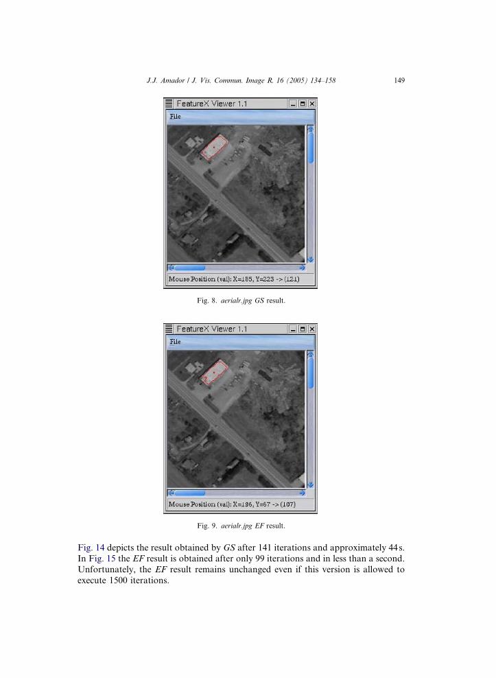
Fig. 8. aerialr.jpg GS result.

Fig. 9. aerialr.jpg EF result.


Fig. 14 depicts the result obtained by GS after 141 iterations and approximately 44s.

In Fig. 15 the EF result is obtained after only 99 iterations and in less than a second.Unfortunately, the EF result remains unchanged even if this version is allowed to

execute 1500 iterations.

Fig. 10. aerial2.jpg 30 · 25 Hypothesis.

Fig. 11. aerial2.jpg GS result.


Testing and comparing the two code versions now focuses on detecting parts in

images. The first image, sts26r.jpg, contains a trunnion in its left-hand side whichholds a satellite within the space shuttle�s payload bay. The initial hypothesis for

the trunnion is shown in Fig. 16 with GS and EF results shown in Figs. 17

Fig. 12. aerial2.jpg EF result.

Fig. 13. area51.jpg 45 · 50 Hypothesis.


and 18, respectively. The delineation achieved by GS predominantly extracts the

trunnion, alternatively EF is unable. The last image, called ov103.jpg, has its desiredobject located in the upper-left-hand corner. Fig. 19 shows the initial MRF config-

uration used of incorrect size and orientation. Fig. 20 is the GS result obtained after

Fig. 14. area51.jpg GS result (Note. a = 1.0, b = 0.06, c = 0.1).

Fig. 15. area51.jpg EF result (Note. a = 1.0, b = 0.06, c = 0.1).


154 iterations and 17.16s. Fig. 21 depicts the EF result after 202 iterations and 1.05s.

Notice how the GS result is more akin to the object�s shape; the EF result remainsunchanged even if this version executes to 1500 iterations.

Fig. 16. sts26r.jpg 30 · 20 Hypothesis.

Fig. 17. sts26r.jpg GS result (Note. a = 0.5, b = 0.05, c = 0.7).


5.3. Performance comparison

The results provided above were acquired from two different versions of the MRF

algorithm. One uses (3) directly, the other uses the tailored Gibbs Sampler (9). Table 2

Fig. 19. ov103.jpg 30 · 30 Hypothesis.

Fig. 18. sts26r.jpg EF result (Note. a = 0.5, b = 0.05, c = 0.7).


lists the performance metrics between these two versions. For synthetic images there

was no gain in performance or accuracy when using GS over EF. Accordingly, EFachieved practically the same delineation in considerably less time when compared

to GS.

Fig. 21. ov103.jpg EF result (Note. a = 1.0, b = 0.03, c = 0.3).

Fig. 20. ov103.jpg GS result (Note. a = 1.0, b = 0.03, c = 0.3).


For real-world images, the results obtained changes the comparison dramatically.

In all cases GS obtained more precise delineations than EF. Even though EF resultsexecuted faster, the final outcome was not comparable to corresponding GS results.

The reason for this is optimization resulting due to radial sites being bounded by the


high probability zone (i.e., LOWRAD to MAXRAD) utilized as part of the tailored

Gibbs Sampler. The high probability zone allows GS to accurately assign radial sites

to correct edge pixels rather than a random point of high intensity. This of course

increases GS execution time as sites are tested against the high probability zone,

nonetheless, relatively accurate delineations are obtained despite an objects scaleor rotation in an image.

6. Summary

In this paper, given a high-level hypothesis an algorithm for solving region extrac-

tion problems was presented. This new algorithm utilizes probability theory in terms

of Gibbs Distributions and uses a combinatorial optimization technique known asTabu Search. A heuristic energy functional was derived which allows for detecting

quadrilateral- and other compact-closed objects. Since existence of a Gibbs Distribu-

tion is equivalent to the existence of an MRF, if a relevant energy functional can be

derived then a conditional probability environment is created. Thus, defining condi-

tional probabilities is avoided and a particularly useful and easily implemented meth-

od is imparted.

Several series of experiments were conducted on different types of images. Aerial

imagery of buildings and imagery of mechanical parts were empirically studied. Inmost cases the objects were scaled and rotated out of axis-alignment and the initial

MRF configuration (i.e., initial hypothesis) was wrong in all cases. Two versions of

the MRF algorithm were created; one which used a tailored Gibbs Sampler the other

used the energy functional directly. For synthetic images there was no advantage to

using the Gibbs Sampler. However, in all real-world cases the tailored Gibbs Sam-

pler executed superior to the energy-only version. Even though execution time for

energy-only was less, the Gibbs Sampler achieved more accurate results extracting

the desired region in all cases. This was due to sample space convergence into a highprobability configuration despite the initial MRF.

The idea of optimizing an energy functional to find a contour in an image has

been extensively studied (Blake and Isard, 2000). Kass et al. (1988) introduced a class

of active contour model called SNAKES which essentially are controlled continuity

splines. Predominantly, the SNAKES energy functional consists of a linear combina-

tion of three components that attract the ‘‘snake’’ to lines and edges. Energy func-

tional results arrive from integrating along the entire snake, hence, every portion

of the solution is dependent on the entire configuration. Computation-wise, this be-comes an expensive procedure requiring matrix operations that are substantial as the

complexity of the energy functional increases. Alternatively, this paper proposes con-

figuring a collection of radii as an MRF, such that each radius is independently cal-

culated and determined. The energy functional is defined in terms of a radial point,

instead of the entire MRF configuration. Recognition criteria are essentially incor-

porated into an energy functional by exploiting the Gibbs Distribution�s usefulnessfor finding an MRF of highest probability. Moreover, Tabu Search optimization is

used for finding the energy function�s lowest energy state.


Future considerations include region extraction of more complex shapes, for

example concave in nature. Furthermore, the problem of occluded regions will be

studied.

Acknowledgments

The author thanks the anonymous reviewers for their helpful questions, com-

ments, and insight during the review phase. The author also thanks Jihun Cha for

his exceptional work on the FeatureX Viewer which was instrumental in capturing

the resultant images used in the empirical section. A final thanks goes to Fred Glover

for the initial email correspondence in understanding the short-term memory aspects

of Tabu Search.

References

Aksoy, S., Haralick, R.M., 1999. Graph-theoretic clustering for image grouping and retrieval. In: IEEE

Computer Society Conference on Computer Vision and Pattern Recognition, vol. 1, pp. 63–68.

Al-Sultan, K.S., 1995. A Tabu search approach to the clustering problem. Pattern Recogn. 28 (9), 1443–

1451.

Ball, G.H., Hall, D.J., 1965. ISODATA, A novel method of data analysis and pattern classification.

Information Sciences Branch, Office of Naval Research, Contract No. 4918(00), SRI Project 5533,

Stanford Research Institute, Menlo Park, California.

Besag, J., 1974. Spatial interaction and the statistical analysis of lattice systems. J. R. Stat. Soc. Series B

(36), 192–236.

Blake, A., Isard, M., 2000. Active Contours. Springer-Verlag London Limited, Great Britain.

Canny, J., 1986. A computational approach to edge detection. IEEE Trans. Pattern Anal. Mach. Intell.

PAMI-8 (6), 679–698.

Castleman, K.R., 1996. Digital Image Processing. Prentice Hall, New Jersey.

Cover, T.M., Hart, P.E., 1967. Nearest neighbor pattern classification. IEEE Trans. Inform. Theory IT-13

(1), 21–27.

Cramariuc, B., Gabbouj, M., Astola, J., 1997. Clustering based region growing algorithm for color image

segmentation. In: Thirteenth International Conference onDigital Signal Processing, vol. 2, pp. 857–860.

Cross, G.R., Jain, A.K., 1983. Markov random field texture models. IEEE Trans. Pattern Anal. Mach.

Intell. PAMI-5 (1), 25–39.

Delagnes, P., Barba, D., 1996. Rectilinear structure extraction in textured images with an irregular, graph-

based Markov random field model. In: Thirteenth International Conference on Pattern Recognition,

vol. 2, pp. 800–804.

Duda, R.O., Hart, P.E., 1973. Pattern Classification and Scene Analysis. Wiley, New York.

da Fortuna Costa, L., Cesar Jr., R.M., 2001. Shape Analysis and Classification. CRC Press, Boca Raton,

FL.

Geman, S., Geman, D., 1984. Stochastic Relaxation, Gibbs Distributions, and the Bayesian Restoration of

Images. IEEE Trans. Pattern Anal. Mach. Intell. PAMI-6 (6), 721–741.

Glover, F., 1989. Tabu Search—part I. ORSA J. Comput. 1 (3), 190–206.

Glover, F., 1990. Tabu Search: a tutorial. Interfaces 20, 74–94.

Glover, F., Laguna, M., 1997. Tabu Search. Kluwer Academic Publishers, Boston.

Gunsel, B., Panayirci, E., Jain, A.K., 1994. Boundary detection using multiscale Markov random fields.

In: Twelfth IAPR International Conference on Vision and Signal Image Processing, vol. 2, pp. 173–

177.


Hill, A., Taylor, C.J., 1992. Model-based image interpretation using genetic algorithms. Image Vision

Comput. 10 (5), 295–300.

Kass, M., Witkin, A., Terzopoulos, D., 1988. Snakes: active contour models. Int. J. Comput. Vision 1,

321–331.

Li, S.Z., 1994. A Markov random field model for object matching under contextual constraints. In: IEEE

Computer Society Conference on Computer Vision and Pattern Recognition, pp. 63–68.

Margalit, A., Rosenfeld, A., 1990. Using probabilistic domain knowledge to reduce the expected

computational cost of template matching. Comput. Vision Graph. Image Process. 51, 219–234.

Modestino, J.W., Zhang, J., 1992. A Markov random field model-based approach to image interpretation.

IEEE Trans. Pattern Anal. Mach. Intell. 14 (6), 606–615.

Maniezzo, V., Dorigo, M., Colorni, A., 1995. Algodesk: an experimental comparison of eight evolutionary

heuristics applied to the quadratic assignment problem. Eur. J. Oper. Res. 81, 188–204.

Nadabar, S.G., Jain, A.K., 1996. Parameter estimation in markov random field contextual models using

geometric models of objects. IEEE Trans. Pattern Anal. Mach. Intell. 18 (3), 326–329.

Pirlot, M., 1996. General local search methods. Eur. J. Oper. Res. 92, 493–511.

Roberts, L.G., 1965. Machine perception of three-dimensional solids. In: Tippett, J.T. (Ed.), Optical and

Electro-Optical Information Processing. MIT Press, Cambridge, MA, pp. 159–189.

Sinclair, M., 1993. Comparison of the performance of modern heuristics for combinatorial optimization

on real data. Comput. Oper. Res. 20 (7), 687–695.

Schluter, D., Wachsmuth, S., Sagerer, G., 2000. Towards an integrated framework for contour-based

grouping and object recognition using Markov random fields. In: International Conference on Image

Processing, vol. 2, pp. 100–103.

Tomasi, C., Manduchi, R., 1998. Stereo matching as a nearest-neighbor problem. IEEE Trans. Pattern

Anal. Mach. Intell. 20 (3), 333–340.

markov random field approach to region extraction using tabu search

Documents