markov chain analysis of succession in a rocky subtidal community

The University of Chicago

Markov Chain Analysis of Succession in a Rocky Subtidal Community.Author(s): M. Forrest Hill, Jon D. Witman, and Hal CaswellSource: The American Naturalist, Vol. 164, No. 2 (August 2004), pp. E46-E61Published by: The University of Chicago Press for The American Society of NaturalistsStable URL: http://www.jstor.org/stable/10.1086/422340 .

Accessed: 10/04/2014 03:00

Your use of the JSTOR archive indicates your acceptance of the Terms & Conditions of Use, available at .http://www.jstor.org/page/info/about/policies/terms.jsp

.JSTOR is a not-for-profit service that helps scholars, researchers, and students discover, use, and build upon a wide range ofcontent in a trusted digital archive. We use information technology and tools to increase productivity and facilitate new formsof scholarship. For more information about JSTOR, please contact [email protected].

.

The University of Chicago Press, The American Society of Naturalists, The University of Chicago arecollaborating with JSTOR to digitize, preserve and extend access to The American Naturalist.

http://www.jstor.org

This content downloaded from 83.249.7.62 on Thu, 10 Apr 2014 03:00:08 AMAll use subject to JSTOR Terms and Conditions

http://www.jstor.org/action/showPublisher?publisherCode=ucpress

http://www.jstor.org/action/showPublisher?publisherCode=amsocnat

http://www.jstor.org/stable/10.1086/422340?origin=JSTOR-pdf

http://www.jstor.org/page/info/about/policies/terms.jsp


vol. 164, no. 2 the american naturalist august 2004

E-Article

Markov Chain Analysis of Succession in a Rocky

Subtidal Community

M. Forrest Hill,1,* Jon D. Witman,2,† and Hal Caswell3,‡

1. Institute of Theoretical Dynamics, University of California,Davis, California 95616;2. Department of Ecology and Evolutionary Biology, BrownUniversity, Providence, Rhode Island 02912;3. Biology Department MS-34, Woods Hole OceanographicInstitution, Woods Hole, Massachusetts 02543

Submitted June 18, 2003; Accepted February 24, 2004;Electronically published July 1, 2004

abstract: We present a Markov chain model of succession in arocky subtidal community based on a long-term (1986–1994) studyof subtidal invertebrates (14 species) at Ammen Rock Pinnacle inthe Gulf of Maine. The model describes successional processes (dis-turbance, colonization, species persistence, and replacement), theequilibrium (stationary) community, and the rate of convergence.We described successional dynamics by species turnover rates, re-currence times, and the entropy of the transition matrix. We usedperturbation analysis to quantify the response of diversity to suc-cessional rates and species removals. The equilibrium communitywas dominated by an encrusting sponge (Hymedesmia) and a bryo-

zoan (Crisia eburnea). The equilibrium structure explained 98% ofthe variance in observed species frequencies. Dominant species havelow probabilities of disturbance and high rates of colonization andpersistence. On average, species turn over every 3.4 years. Recurrencetimes varied among species (7–268 years); rare species had the longestrecurrence times. The community converged to equilibrium quickly(9.5 years), as measured by Dobrushin’s coefficient of ergodicity. Thelargest changes in evenness would result from removal of the dom-inant sponge Hymedesmia. Subdominant species appear to increaseevenness by slowing the dominance of Hymedesmia. Comparison ofthe subtidal community with intertidal and coral reef communitiesrevealed that disturbance rates are an order of magnitude higher incoral reef than in rocky intertidal and subtidal communities. Col-onization rates and turnover times, however, are lowest and longest

* Present address: ENTRIX, 590 Ygnacio Valley Road, Walnut Creek, Cali-

fornia 94596; e-mail: [email protected].

† E-mail: [email protected].

‡ Corresponding author; e-mail: [email protected].

Am. Nat. 2004. Vol. 164, pp. E46–E61. � 2004 by The University of Chicago.0003-0147/2004/16402-30238$15.00. All rights reserved.

in coral reefs, highest and shortest in intertidal communities, andintermediate in subtidal communities.

Keywords: Markov chain, sensitivity analysis, transition matrix, spe-cies diversity, entropy, Dobrushin’s coefficient.

The dynamics of an ecological community are often de-scribed by changes in species composition over time. Weuse the term “succession” to refer to these changes. Suc-cession is no longer viewed as a deterministic developmenttoward a unique stable climax community (Connell andSlatyer 1977). Instead, it is widely recognized that distur-bance, dispersal, colonization, and species interactionsproduce patterns and variability on a range of temporaland spatial scales.

Markov chains were introduced as models of successionby Waggoner and Stephens (1970) and Horn (1975). Thesemodels imagine the landscape as a large (usually infinite)set of patches or points in space. The state of a point isgiven by the list of species that occupy it. In one class ofmodels, this list may include multiple coexisting popu-lations; such models are called patch-occupancy models(e.g., Caswell and Cohen 1991a, 1991b). In another classof models, points are occupied by single individuals ratherthan populations. Such models have been applied to forests(Waggoner and Stephens 1970; Horn 1975; Runkle 1981;Masaki et al. 1992), plant communities (Isagi and Naka-goshi 1990; Aaviksoo 1995), insect assemblages (Usher1979), coral reefs (Tanner et al. 1994, 1996), and rockyintertidal communities (Wootton 2001b, 2001c).

Successional dynamics are modeled by defining theprobability distribution of the patch state at time ,t � 1conditional on its state at time t. This distribution maydepend on time, location, and local or global state fre-quencies. Time-varying models can be analyzed as non-homogeneous Markov chains (e.g., Hill et al. 2002). Mod-els with dependence on local state frequencies arenonlinear stochastic cellular automata (e.g., Caswell andEtter 1999). Models with dependence on global state fre-quencies are nonlinear Markov chains (Caswell and Cohen



Markov Chain Analysis of Succession E47

1991a, 1991b; Hill 2000), which are mean-field models forthe corresponding cellular automata.

Models with time-invariant transition probabilities arehomogeneous, finite-state Markov chains. Here, we usesuch a chain to analyze succession in a rocky subtidalcommunity. A detailed statistical analysis of the model thatexamined the effects of spatial and temporal variationshowed that although statistically significant, the effectsare so small as to be biologically trivial, regardless ofwhether asymptotic or transient properties of the com-munity are examined (Hill et al. 2002). We will explorethe effects of nonlinearity elsewhere.

Suppose that there are s possible states. Let X(t) �denote the state of a point at time t. The model{1, 2, … , s}

is defined by a transition matrix P, whose elements, ,pij

are the conditional probabilities:

p p P[X(t � 1) p iFX(t) p j] i, j p 1, … , s. (1)ij

P is column-stochastic (i.e., each column sums to 1). Letx be a probability vector (i.e., whosex ≥ 0, � x p 1)i ii

entries give the probability that a point is in state i. Then

x(t � 1) p Px(t). (2)

If the community is conceived of as an ensemble of points,each experiencing an independent realization of the sto-chastic process given by P, then x(t) defines the state ofthe community; its entries are the expected relative fre-quencies of point states at time t.

We believe that Markov chain models are a valuable butunderutilized tool in community ecology. Consequently,one of our goals is to extend the analysis of communitydynamics by a more systematic exploration of the prop-erties of Markov chain models than has appeared in anyprevious study. This is the first time that some of theseresults have been reported for any community. To helpinterpret them, we will contrast our results with thoseobtained from matrices reported by Wootton (2001c) forintertidal communities in Washington and by Tanner etal. (1994) for coral reefs in Australia. Such comparativeanalysis will become more powerful and more valuable asadditional data sets are collected (see Wootton 2001a fora comparison along different lines from ours).

The Subtidal Community

Rocky subtidal habitats extend from the intertidal areadown to the upper limit of the deep sea at about 200 m(Witman and Dayton 2001). Here we will study a subtidalcommunity on vertical rock walls; such communities aredominated by epifaunal invertebrates (Sebens 1986). Theyare subject to lower disturbance rates than communities

on horizontal substrates at similar depths. Witman andDayton (2001) have reviewed the processes (disturbance,predation, and competition) operating in these commu-nities. Because sessile organisms require substrate, com-petition for space plays a key role; disturbance and pre-dation open up space for colonization. Colonizationusually requires recruitment of larvae. At shallow subtidaldepths, larvae sometimes settle in dense aggregations thatcompletely cover available space, but this seems to happenless often at deeper depths, including the depths fromwhich our data come (Witman and Dayton 2001).

Subtidal succession has typically been studied on small(!0.1 m2) artificial substrata such as plates or tiles (Suth-erland and Karlson 1977; Osman 1982), so there are fewstudies of succession on natural hard substrates for com-parison. Keough (1984) found that the dynamics of sessileepifauna on fan-shaped shells of a large bivalve were dom-inated by recruitment, with high species turnover as res-idents died. Disturbance was low in these small, discretehabitats. Physical disturbance had a greater influence onepifaunal communities on shallow (4–12-m depth) rockwalls in the Caribbean, where the communities were im-pacted three times in six years by hurricanes, which createdsmall patches (!25 cm2) for succession (Witman 1992).Since wave energy dissipates with depth, natural physicaldisturbance should decrease with depth in the rocky sub-tidal community (Witman and Dayton 2001).

Parameter Estimation

Our analysis focuses on a subtidal rock wall communityat 30–35-m depth on Ammen Rock Pinnacle in the centralGulf of Maine (Witman and Sebens 1988; Leichter andWitman 1997). Nine permanently marked 0.25-m2 quad-rats, positioned horizontally along a 20-m span of the rockwall habitat, were photographed each year with a Nikonoscamera mounted on a quadrapod frame (Witman 1985).A total of 14 species of sponges, sea anemones, ascidians,bryozoans, and polychaetes were identified in the photos(table 1). For reasons that will become apparent, we haveordered the species in decreasing rank order of dominancein the equilibrium community.

Transition frequencies were measured by superimpos-ing a rectangular lattice of points at 1-cm in-30 # 20tervals onto -cm color prints made from high-31.25 # 20resolution color slides of the quadrat photos. Thiscorresponds to approximately a 2-cm interval on the ac-tual substrate ( ), which approxi-1/2[0.25/0.06] p 2.04mates the size of the smallest organisms in the data set.At each time, the lattice was aligned to assure that specieswere always censused at the same points. We recordedthe species occupying each point on each quadrat in eachyear, for a total of ∼42,000 points (the species occupying



E48 The American Naturalist

Table 1: Subtidal species found in quadrats at 30-m depth onAmmen Rock Pinnacle in the Gulf of Maine

Model states Species type State ID Number

Hymedesmia sp. 1 Sponge HY1 14,875Crisia eburnea Bryozoan CRI 9,915Myxilla fimbriata Sponge MYX 4,525Mycale lingua Sponge MYC 3,001Filograna implexa Polychaete FIL 2,219Urticina crassicornis Sea anemone URT 992Ascidia callosa Ascidian ASC 1,052Aplidium pallidum Ascidian APL 1,166Hymedesmia sp. 2 Sponge HY2 1,226Idmidronea atlantica Bryozoan IDM 730Coralline Algae Encrusting algae COR 875Metridium senile Sea anemone MET 1,298Parasmittina jeffreysi Bryozoan PAR 402Spirorbis spirorbis Polychaete SPI 225Bare rock BR 4,266

Note: Species are identified in the model using the state codes listed under

State ID. Number of points counted per species is shown in the right-hand

column of the table. Species are listed in decreasing order of abundance in

the stationary community.

a few points were unidentifiable; these points were ex-cluded from the analysis). The state of a point is givenby the species (or bare rock) that occupies it; thus thereare 15 possible states in our model. Table 1 shows thenumber of sampled points in each state and the abbre-viations used to identify each state.

Maximum likelihood estimates of transition probabil-ities were obtained by creating a contingency table inwhich the i, j entry, nij, gives the number of points thatwere in state j at time t and state i at . The transitiont � 1probabilities, pij, were estimated as

nijp p . (3)ij � niji

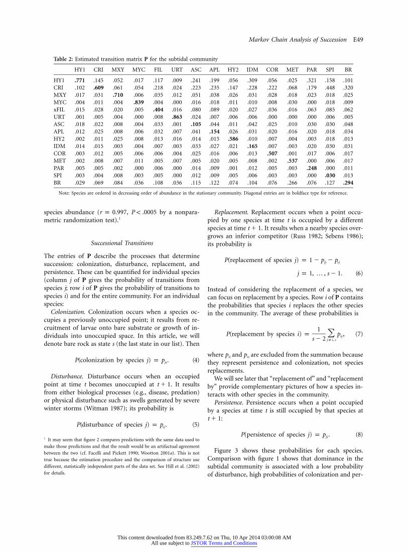
These estimates average over spatial and temporal vari-ability to produce the best single estimate of a homogenousMarkov chain for the subtidal community. The resultingtransition matrix is shown in table 2.

We will extract three levels of information from themodel:

Species properties. These describe aspects of the biologyof an individual species in the context of its community.For example, the probability that an empty point is col-onized by the bryozoan Crisia eburnea is .32, while thecorresponding probability for the polychaete Spirorbis spi-rorbis is only .01. Crisia is one of the most abundant speciesin the equilibrium community; Spirorbis is one of the rar-est. We will use such comparisons to see to what extent

species-specific properties are correlated with equilibriumabundance.

Community properties. These describe properties of theentire community rather than those of individual species.Some of them are obtained by averaging species propertiesover the equilibrium community composition. For ex-ample, the average time before a randomly selected pointin the subtidal community changes state (its turnovertime) is 3.4 years. We can compare such community prop-erties with the corresponding properties of othercommunities.

Perturbation properties. These describe how changes ineither the transition structure or the species pool wouldaffect the resulting community. There are many such ques-tions; we will focus on a small subset concerned with thediversity and evenness of the community.

Successional Analysis

Stationary Community Structure

We begin by using P to calculate the stationary, or equi-librium, community structure. If the transition matrix Pis primitive (i.e., if for some finite ), then akP 1 0 k ≥ 1community described by equation (2) will asymptoticallyapproach an equilibrium, or stationary, probability dis-tribution from any initial condition. This distribution isgiven by the dominant eigenvector of P, normalized tosum to 1; we denote this eigenvector as w. Many authorshave focused on the stationary distribution as a predictionof asymptotic community composition (e.g., Waggonerand Stephens 1970; Usher 1979; Rego et al. 1993; Gibsonet al. 1997; Wootton 2001b, 2001c).

Figure 1 shows the stationary structure of the subtidalcommunity, with the biological species listed in decreasingorder of abundance and bare rock at the end. By listingthe species this way, correlations of species properties withabundance will be clearly visible in subsequent figures. Thedominant species are the encrusting sponge Hymedesmiasp. 1, which occupies 34% of the substrate, and the erectbryozoan Crisia eburnea, which occupies 26% of the sub-strate. The remaining 12 species occupy 33.5% of the sub-strate, with frequencies ranging from 7.6% (Myxilla fim-briata) down to 0.5% (Spirorbis spirorbis). About 8.0% ofthe substrate is unoccupied.

The stationary structure computed from P agrees re-markably well with the observed structure of the subtidalcommunity (fig. 2), explaining 98% of the variance in




Table 2: Estimated transition matrix P for the subtidal community

HY1 CRI MXY MYC FIL URT ASC APL HY2 IDM COR MET PAR SPI BR

HY1 .771 .145 .052 .017 .117 .009 .241 .199 .056 .309 .056 .025 .321 .158 .101CRI .102 .609 .061 .054 .218 .024 .223 .235 .147 .228 .222 .068 .179 .448 .320MXY .017 .031 .710 .006 .035 .012 .051 .038 .026 .031 .028 .018 .023 .018 .025MYC .004 .011 .004 .839 .004 .000 .016 .018 .011 .010 .008 .030 .000 .018 .009xFIL .015 .028 .020 .005 .404 .016 .080 .089 .020 .027 .036 .016 .063 .085 .062URT .001 .005 .004 .000 .008 .863 .024 .007 .006 .006 .000 .000 .000 .006 .005ASC .018 .022 .008 .004 .033 .001 .105 .044 .011 .042 .025 .010 .030 .030 .048APL .012 .025 .008 .006 .032 .007 .041 .154 .026 .031 .020 .016 .020 .018 .034HY2 .002 .011 .025 .008 .013 .016 .014 .015 .586 .010 .007 .004 .003 .018 .013IDM .014 .015 .003 .004 .007 .003 .033 .027 .021 .165 .007 .003 .020 .030 .031COR .003 .012 .005 .006 .006 .004 .025 .016 .006 .013 .507 .001 .017 .006 .017MET .002 .008 .007 .011 .005 .007 .005 .020 .005 .008 .002 .537 .000 .006 .017PAR .005 .005 .002 .000 .006 .000 .014 .009 .001 .012 .005 .003 .248 .000 .011SPI .003 .004 .008 .003 .005 .000 .012 .009 .005 .006 .003 .003 .000 .030 .013BR .029 .069 .084 .036 .108 .036 .115 .122 .074 .104 .076 .266 .076 .127 .294

Note: Species are ordered in decreasing order of abundance in the stationary community. Diagonal entries are in boldface type for reference.

species abundance ( , by a nonpara-r p 0.997 P ! .0005metric randomization test).1

Successional Transitions

The entries of P describe the processes that determinesuccession: colonization, disturbance, replacement, andpersistence. These can be quantified for individual species(column j of P gives the probability of transitions fromspecies j; row i of P gives the probability of transitions tospecies i) and for the entire community. For an individualspecies:

Colonization. Colonization occurs when a species oc-cupies a previously unoccupied point; it results from re-cruitment of larvae onto bare substrate or growth of in-dividuals into unoccupied space. In this article, we willdenote bare rock as state s (the last state in our list). Then

P(colonization by species j) p p . (4)js

Disturbance. Disturbance occurs when an occupiedpoint at time t becomes unoccupied at . It resultst � 1from either biological processes (e.g., disease, predation)or physical disturbance such as swells generated by severewinter storms (Witman 1987); its probability is

P(disturbance of species j) p p . (5)sj

1 It may seem that figure 2 compares predictions with the same data used to

make those predictions and that the result would be an artifactual agreement

between the two (cf. Facelli and Pickett 1990; Wootton 2001a). This is not

true because the estimation procedure and the comparison of structure use

different, statistically independent parts of the data set. See Hill et al. (2002)

for details.

Replacement. Replacement occurs when a point occu-pied by one species at time t is occupied by a differentspecies at time . It results when a nearby species over-t � 1grows an inferior competitor (Russ 1982; Sebens 1986);its probability is

P(replacement of species j) p 1 � p � pjj sj

j p 1, … , s � 1. (6)

Instead of considering the replacement of a species, wecan focus on replacement by a species. Row i of P containsthe probabilities that species i replaces the other speciesin the community. The average of these probabilities is

1P(replacement by species i) p p , (7)� ijs � 2 j(i, s

where pii and pis are excluded from the summation becausethey represent persistence and colonization, not speciesreplacements.

We will see later that “replacement of” and “replacementby” provide complementary pictures of how a species in-teracts with other species in the community.

Persistence. Persistence occurs when a point occupiedby a species at time t is still occupied by that species at

:t � 1

P(persistence of species j) p p . (8)jj

Figure 3 shows these probabilities for each species.Comparison with figure 1 shows that dominance in thesubtidal community is associated with a low probabilityof disturbance, high probabilities of colonization and per-




Figure 1: Stationary distribution of species frequencies in the subtidal community. Species are displayed in decreasing order of abundance, withbare rock (BR) at the end.

sistence, a high probability of replacing other species (“re-placement by”), and a low probability of being replacedby other species (“replacement of”). The positive corre-lations of dominance with colonization and the probabilityof “replacement by” are statistically significant (table 3).

Successional transitions can also be examined at thelevel of the community:

Colonization. The probability that an empty point iscolonized by some species is

P(colonization) p p p 1 � p� is ssi(s

p 0.71. (9)

Disturbance. The probability that an occupied point,randomly selected from the stationary community, is dis-turbed between t and is the average over the sta-t � 1tionary distribution of the species-specific disturbanceprobabilities:

� w pj sjj(sP(disturbance) p � wj

j(s

p 0.06. (10)

Replacement. The probability that a point, randomly se-lected from the stationary community, is replaced by adifferent species is the average over the stationary distri-bution of the probability of replacement:

� w (1 � p � p )i ii sii(sP(replacement of) p � wi

i(s

p 0.29. (11)

Equation (7) gives the average probability of replacementby species i. The average of this quantity over the stationarydistribution gives

1 � w � pi ijs�2 i(s j(i, sP(replacement by) p � wi

i(s

p 0.10. (12)

Note that the choice to exclude bare rock (state s) fromthe averages in equations (11) and (13) is a choice of




Figure 2: Left, Stationary distribution and the observed frequency distribution of species in the subtidal community. Species are displayed indecreasing order of abundance in the stationary distribution and in the order shown in figure 1. Right, Observed species frequencies as a functionof the frequencies in the stationary distribution. The correlation between the observed and stationary distribution is ; by ar p 0.9838 P ! .0005nonparametric permutation test.

interpretation; most ecologists would be concerned withcolonization, disturbance, and replacement of biologicalspecies only, but there is no reason that comparable av-erages could not be calculated including bare rock or forother subsets of the community (e.g., all sponges).

In the subtidal community, the rate of disturbance islow (0.06), the colonization rate is high (0.71), and thereplacement rate is intermediate (0.29). In “A ComparativeAnalysis of Benthic Communities,” we will compare thesevalues to other communities.

Successional Dynamics

Turnover Rates. The turnover rate measures the rate atwhich points change state and is thus one measure of therate of successional change. The turnover rate of speciesi is the probability that a point in state i changes statebetween t and ; it ist � 1

T p (1 � p ). (13)i ii

The inverse of the turnover rate gives the expected turn-over time of species i:

1E(turnover time) p t p . (14)i Ti

Figure 4 shows these turnover times. Most are short (≤2

years); the longest are 6.2 and 7.3 years. There is a positivebut nonsignificant correlation of turnover time with dom-inance in the stationary community (table 3).

The mean turnover time of a point in the stationarycommunity is the average over the stationary distributionof the :ti

swi

t p . (15)� Tip1 i

This includes the turnover time of bare rock (state s).Calculating the mean over only occupied points producesthe biotic turnover time:

wi� T ii(st p . (16)bio � wi

i(s

In the subtidal community, years.t p 3.4bio

Recurrence Times. A point in any state will eventually leavethat state and then return to it at some later time. TheSmoluchowski recurrence time of state i is the averagetime elapsing between a point leaving state i and thenreturning to it again. It is given by




Figure 3: Species-specific transition probabilities from the community transition matrix P for the subtidal community. Species are displayed indecreasing order of abundance in the stationary distribution, in the order shown in figure 1. a, Probability that the species is disturbed in one unitof time. b, Probability that the species colonizes a patch of bare rock in one unit of time. c, Probability that a species persists for one unit of time.d, Average probability of replacement of other species. e, Probability that the species is replaced by some other species.

1 � wiv p (17)i w (1 � p )i ii

(Iosifescu 1980). These recurrence times are highly variableamong species in the subtidal community, ranging from7.1 to 268.5 years (fig. 4). There is a significant negativecorrelation between and abundance in the stationaryvi

community ( , ; see table 3); that is,r p �0.55 P p .026the rarer a species is, the longer it takes for that speciesto reoccupy a point.

In the stationary community, the mean recurrence timeis

v p w v , (18)� i ii

and the biotic mean recurrence time is

� w vi ii(s

v p . (19)bio � wii(s

In the subtidal community, the mean recurrence time isyears, and the biotic mean recurrence time isv p 36.2

years.v p 37.9bio

The recurrence time for bare rock is the mean time thata point remains occupied once it has been colonized andis thus the mean time between disturbances. In the subtidalcommunity, this is years. Since the biotic meanv p 16.2s

turnover time years, a point changes its bioticT p 3.4bio

state an average of times between16.2/3.4 p 4.8disturbances.

Entropy, Complexity, and Predictability of Succession. Intheir study of coral reef succession, Tanner et al. (1994)noted that between 88% and 91% of the entries of P werepositive; they called this high proportion of nonzero en-




Table 3: Correlations between species prop-erties and species abundance in the station-ary community structure

Variable r P

Transition probabilities:Disturbance �.2605 .3325Colonization .6035 .0150Persistence .4203 .1135Replacement of �.3791 .1590Replacement by .9277 .0010

Dynamic properties:Turnover time .2416 .3990Recurrence time �.5525 .0265Species entropy �.3383 .2070

Perturbation properties;elasticity of H to:

Disturbance .8063 .0050Colonization �.8922 .0045Persistence �.8474 .0040Replacement of .9075 .0060Replacement by �.9153 .0025

Note: P values are for tests of the null hypothesis

of no correlation between the property in question

and abundance, computed with a randomization test.

Correlations were calculated for 2,000 random per-

mutations of the species property; P is the proportion

of the resulting 2,001 correlations greater than or

equal in absolute magnitude to the observed

correlation.

tries the “most remarkable aspect” of their transition ma-trices and defined it as a “complexity index.” The subtidalcommunity has a similarly high complexity index (95%).

However, the complexity index provides only limitedinformation on succession because it is insensitive to themagnitude of the transition probabilities. Consider the col-umn of P giving the transition probabilities for species j.The complexity index does not distinguish between

0.25 0.01 0.25 0.97

p p and p p (20).j .j0.25 0.01 0.25 0.01

because both have a complexity index of 1.0. But in thefirst case, the fate of a point occupied by species j is com-pletely uncertain, while in the second it is almost certainthat species j will be replaced by species 2.

An index that takes into account not only the propor-tion of nonzero entries but also their relative magnitudesis the entropy of p.j:

H(p ) p � p log p . (21)�.j ij iji

The entropies of the two columns in equation (20) are1.38 and 0.17. Thus the entropy of a species is an inversemeasure of the predictability of its successional changes.

The species entropies for the subtidal community rangefrom 0.69 to 2.2 (the maximum possible value is

; fig. 4). There is a negative but nonsignificantlog 15 p 2.7correlation between species entropy and dominance in thestationary community (table 3).

The entropy of the Markov chain as a whole (e.g., Khin-chin 1957; Reza 1961) is the average over the stationarydistribution of the entropies of the columns of P:

s s

H(P) p � w p log p . (22)� �j ij ijjp1 ip1

The quantity H(P) gives the uncertainty in the fate of apoint randomly selected from the stationary community.If , the state of a point in the next time step isH(P) p 0completely known (i.e., the uncertainty is 0), and succes-sion is completely deterministic. The maximum uncer-tainty occurs when , in whichH(P) p H (P) p log (1/s)max

case the fate of a point is completely unpredictable. SinceHmax(P) depends on s, we can calculate the normalizedentropy of P as

H(P)H (P) p . (23)r H (P)max

The normalized entropy of the subtidal transition matrixis . This community is poised halfway be-H (P) p 0.49r

tween predictability and unpredictability.

Community Convergence

The rate of convergence to the stationary distribution canbe measured in several ways (Cohen et al. 1993; Rosenthal1995). One is the damping ratio

l1r p , (24)

Fl F2

where and are the largest and second-largest eigen-l l1 2

values of P (because P is stochastic, ). Communityl p 11

structure converges to the equilibrium, in the long run,at least as fast as (Caswell 2001), so r pro-exp (�t log r)vides a lower bound on the convergence rate. The closerthe second eigenvalue is in magnitude to the first, theslower the rate of convergence. The half-life of a pertur-bation is given by . The damping ratio has beenlog 2/ log r

applied to succession models by Tanner et al. (1994) andWootton (2001c).

An alternative measure of convergence rate, not re-




Figure 4: Species-specific dynamic properties of the subtidal community. Species are displayed in decreasing order of abundance in the stationarydistribution, in the order shown in figure 1. a, Turnover time (years). b, Smoluchowski recurrence time (years). c, Entropy of the column in thetransition matrix P corresponding to each species.

stricted to asymptotic conditions, is provided by Dob-rushin’s coefficient of ergodicity (Dobrushin 1956a,a(P)1956b). Imagine two copies of the same community start-ing from initial states x1 and x2. After one iteration thenew states Px1 and Px2 will be closer together than x1 andx2 were, and the amount of contraction is given by

kPx � Px k1 2 , (25)kx � x k1 2

where denotes the 1-norm. Dobrushin’s coefficient,k 7 k

kPx � Px k1 2a(P) p sup , (26)( )kx � x kx , x 1 21 2

gives an upper bound on the contraction, and hencegives a lower bound on the convergence rate,¯� log a(P)

comparable to . Dobrushin’s coefficient is calculatedlog r

from P as

1a(P) p max kp � p k, (27).j .k2 j, k

where p.j is column j of P.Unlike the damping ratio, Dobrushin’s coefficient re-

veals an important connection between the transitionprobabilities and the convergence rate. Dobrushin’s co-efficient depends on the differences among the columnsof P, each of which is the probability distribution of thefate of a point occupied by one of the species. If all thespecies behave identically, then all the columns of P areidentical, , and the community converges to itsa(P) p 0stationary distribution in a single iteration. At the otherextreme, if the species have completely different fates, then

and the only possible stochastic matrix is onea(P) p 1that cycles deterministically among the states, and thecommunity never converges. The convergence rate of thecommunity is thus inversely related to the ecological dif-ferences among the species.




In the subtidal community, , implying a con-r p 1.16vergence rate of (i.e., ∼15%/year) and a half-log r p 0.15life of 4.7 years. Dobrushin’s coefficient is , im-a p 0.89plying a short-term convergence rate of ¯� log a p 0.12(∼12%/year).

Perturbation Analysis

Perturbation analysis plays an essential role in demo-graphic analysis (Tuljapurkar and Caswell 1997; Caswell2001) and can be equally valuable in community modeling.In this section we examine the elasticity of species diversityto changes in the pij and the effects on evenness of elim-inating a species from the community. Many other per-turbation analyses are possible.

Changes in Transition Probabilities

Eigenvector sensitivity analysis permits the calculation ofthe effects on diversity of perturbations to P. The station-ary community composition is given by the dominanteigenvector w1 of P, scaled to sum to 1. The sensitivity ofthis scaled eigenvector to changes in the transition prob-ability pij is

w1�kw k �w �w1 1 kp � w , (28)�1�p �p �pkij ij ij

where

s (m)�w v1 i(1)p w w . (29)�j m�p l � lm(1ij 1 m

Here, is the element of w1, is element i of the(m)(1)w jth vj i

left eigenvector vm, and is the mth eigenvalue (see Cas-lm

well 2001, section 9.4). However, equation (29) cannot bedirectly applied to Markov chain models (as attempted byTanner et al. [1994]) because in the context of Markovchains, the only perturbations of interest are those thatpreserve the column sums of P, which must equal 1. Thusany change in pij must be accompanied by compensatingchanges in the other entries of column j. The resultingtotal derivative is

w w1 1w1 � �sd kw k kw k kw k �p1 1 1 mjp � (30)�dp �p �p �pm(iij ij mj ij

(Caswell 2001). In equation (30), the derivativesfor are determined so that the change in�p /�p m ( imj ij

pij is compensated for by changes in the other entries in

column j of P. While several compensation patterns arepossible (see Caswell 2001 for details), here we use pro-portional compensation:

�p �pmj mjp m ( i, (31)�p 1 � pij ij

in which the change in pij is distributed over the otherentries in the jth column proportional to their value. Othercompensation methods give qualitatively similar results.

We use the eigenvector sensitivities (eq. [30]) to com-pute the sensitivity of the Shannon-Wiener diversity index.This index is usually calculated only over the biotic states,that is, excluding bare rock. The stationary proportions ofthe biotic states are

wi′w p i ( s, (32)i 1 � ws

and the Shannon-Wiener index is the entropy of w′:

′ ′ ′H(w ) p � w log w . (33)� i ii

The sensitivity of H(w′) to changes in pij is

′dH dwi′p � (1 � log w ) , (34)� idp dpiij ij

where

′dw (1 � w )dw /dp � (w )dw /dpi s i ij i s ijp , (35)2dp (1 � w )ij s

and is the mth element of the vector given bydw /dpm ij

equation (30).We will focus on the elasticities, or proportional sen-

sitivities of H, given by

p �Hij .H �pij

The elasticity of H to proportional changes in a set oftransitions (e.g., the probabilities that a species is replacedby another) is simply the sum of the elasticities of H tothose transitions. For example, the elasticity of H to theprobability that species j is replaced by some other speciesis

p �Hij . (36)�H �pi(j, s ij

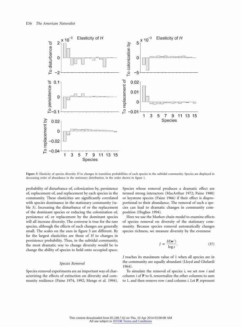
Figure 5 shows the elasticities of H to changes in the




Figure 5: Elasticity of species diversity H to changes in transition probabilities of each species in the subtidal community. Species are displayed indecreasing order of abundance in the stationary distribution, in the order shown in figure 1.

probability of disturbance of, colonization by, persistenceof, replacement of, and replacement by each species in thecommunity. These elasticities are significantly correlatedwith species dominance in the stationary community (ta-ble 3). Increasing the disturbance of or the replacementof the dominant species or reducing the colonization of,persistence of, or replacement by the dominant specieswill all increase diversity. The converse is true for the rarespecies, although the effects of such changes are generallysmall. The scales on the axes in figure 5 are different. Byfar the largest elasticities are those of H to changes inpersistence probability. Thus, in the subtidal community,the most dramatic way to change diversity would be tochange the ability of species to hold onto occupied space.

Species Removal

Species removal experiments are an important way of char-acterizing the effects of extinction on diversity and com-munity resilience (Paine 1974, 1992; Menge et al. 1994).

Species whose removal produces a dramatic effect aretermed strong interactors (MacArthur 1972; Paine 1980)or keystone species (Paine 1966) if their effect is dispro-portional to their abundance. The removal of such a spe-cies can lead to dramatic changes in community com-position (Hughes 1994).

Here we use the Markov chain model to examine effectsof species removal on diversity of the stationary com-munity. Because species removal automatically changesspecies richness, we measure diversity by the evenness:

′H(w )J p . (37)

log s

J reaches its maximum value of 1 when all species are inthe community are equally abundant (Lloyd and Ghelardi1964).

To simulate the removal of species i, we set row i andcolumn i of P to 0, renormalize the other columns to sumto 1, and then remove row i and column i. Let Pi represent




Figure 6: Proportional change in the biotic evenness J resulting from eliminating species. Species are displayed in decreasing order of abundancein the stationary distribution, in the order shown in figure 1.

the transition matrix when state i is removed, w(i) its sta-tionary distribution, and the corresponding evenness.Ji

The proportional change in evenness is

J � JiDJ p . (38)i J

Figure 6 shows for all species; the effects are relativelyDJi

small, and there is no evidence of a keystone species inthe intertidal community by this measure. The removalof the sponge Myxilla or the bryozoan Crisia would pro-duce the largest declines in evenness (9.7% and 7.8%,respectively). Removing the most abundant species Hy-medesmia sp. 1 would increase evenness, but removing anyof the subdominant species would reduce evenness. Thissuggests that when present, the subdominant species in-crease evenness by slowing dominance by Hymedesmia.

Discussion

Markov chains are a powerful framework for the study ofsuccession. They have permitted us to characterize theasymptotic structure, successional rates, and transitionprocesses in the rocky subtidal community. Using pertur-

bation analyses, we have documented the effects on suc-cession of changes in transition probabilities. In such cal-culations, it is important to restrict perturbations to thosethat maintain the column-stochasticity of the transitionmatrix. When we do so, we find that the elasticities ofdiversity are highest to changes in the persistence of thedominant and subdominant species. Changes in the prob-abilities of disturbance and colonization have muchsmaller effects on diversity. Removal of subdominant spe-cies reduces the evenness of the remaining community,which suggests the existence of second-order effects ofthose subdominants in reducing dominance byHymedesmium.

These results can be thought of as a kind of quantitativefingerprint of a community in terms of its successionalprocesses and can be compared across systems. As an ex-ample, we compare our results to two other marine com-munities by analyzing the matrices reported by Tanner etal. (1994) for coral reefs and Wootton (2001c) for a rockyintertidal community.

A Comparative Analysis of Benthic Communities

Three studies have now used Markov chains to describesuccession in marine benthic communities: our analysis




Table 4: Community properties calculated from transition matrices for three marine benthic communities

Subtidal Intertidal Coral reef EC Coral reef EP Coral reef PC

Mean disturbance rate .06 .02 .39 .41 .36Mean colonization rate .71 .93 .14 .26 .34Mean persistence rate .62 .51 .78 .64 .57Replacement by (biotic) .10 .26 .03 .04 .07Replacement of (biotic) .29 .45 .08 .12 .16Proportion bare rock .08 .02 .74 .61 .51Normalized entropy .49 .52 .34 .25 .21Bio turnover rate .36 .47 .48 .52 .52Bio turnover time (years) 3.4 2.9 4.8 5.2 3.3Bio recurrence time (years) 37.9 14.6 121.3 87.0 38.1BR turnover rate .70 .93 .14 .26 .34BR turnover time (years) 1.43 1.07 7.14 3.84 2.94BR recurrence time (years) 16.3 42.9 5.5 5.3 4.5Number of turnovers between disturbance 4.8 5.1 1.15 1.02 1.36Dobrushin’s coefficient .89 .61 .66 .84 .65Bio evenness .71 .56 .82 .83 .77

Note: Values for the intertidal community are calculated from matrices reported by Wootton (2001a) for a mussel bed community in Washington. Values

for the coral reef communities are calculated from matrices reported by Tanner et al. (1994) in a study on Heron Island, Great Barrier Reef, for an exposed

reef crest (EC), a protected reef crest (PC), and an exposed pool (EP).

of the subtidal community; a study by Tanner et al. (1994)of three coral reef communities on Heron Island, Australia;and a study by Wootton (2001b, 2001c) of a rocky inter-tidal community on the coast of Washington. Comparisonsof successional properties across these communities areinformative (table 4).

Transition Probabilities. There are distinct differences insuccessional processes among the communities. Distur-bance rates are an order of magnitude higher in the coralreef communities than in the subtidal or intertidal com-munities. In contrast, colonization rates are highest in thesubtidal and intertidal communities and lowest in the coralreefs. The combination of a high disturbance rate and alow colonization rate explains why over 50% of the coralsubstrate is unoccupied at equilibrium, compared with 8%for the subtidal communities and 2% for the intertidalcommunities. Rates of replacement (averaged over the bi-otic components of the community) are much lower inthe coral reefs than in the subtidal or intertidalcommunities.

The entropy of succession (eq. [23]) is highest in theintertidal and subtidal communities and much lower inthe coral reef. Thus the successional sequence of a pointis most predictable in the coral reef and less predictablein the intertidal or subtidal communities.

Rates of Succession. Mean biotic turnover rates do notTbio

differ much among the communities. The characteristicturnover times range from 3 to 5 years, shortest in thetbio

intertidal community and longest for coral reefs. The biotic

recurrence times are shortest for the intertidal com-vbio

munity (15 years) and longest for the coral reefs (38–121years). The subtidal community is intermediate, with arecurrence time of 38 years.

The rates of succession for empty points (bare rock)reveal striking differences among the communities. Theturnover rate of bare rock is highest in the intertidal com-munity, where an empty point persists only for an averageof 1.07 years. The subtidal community is not far behind,with a turnover time of 1.43 years. Empty space persistsmuch longer in the coral reef, with turnover times of 3–7 years.

The stationary distribution in the coral reef commu-nities is dominated by open space, which is rare in thesubtidal and intertidal communities. The biotic evennessis highest in the coral reef communities because, of theeight species present, none occupies more than 20% ofthe substrate at equilibrium. In contrast, in the intertidalcommunity approximately two-thirds of the substrate isoccupied by a single species (Mytilus californianus). In thesubtidal community, the two most abundant species oc-cupy 60% of the substrate.

The results in table 4 can be combined into a descriptionof succession in these three communities:

Subtidal. A typical point in the subtidal is disturbedabout every 16 years. It remains empty for about 1.4 yearsbefore being colonized. The species occupying the pointafter colonization change every 3.4 years. Once eliminatedfrom a point, a species returns to the point, on average,in 38 years. A randomly selected point experiences aboutfive species replacements before being disturbed again.




The subtidal community converges to a stationary dis-tribution with 8% bare rock and a biotic evenness of

. Deviations from this stationary state decay atJ p 0.71bio

a rate of at least 12%/year.Intertidal. A typical point in the intertidal community

is disturbed about every 40 years. A disturbed point iscolonized almost immediately; the turnover time of barerock is only 1.07 years. The species occupying the pointchange about every 3 years; once replaced, it takes 15 yearsfor a species to return to a point. A point experiences 15species replacements before it is disturbed and returnedto bare rock.

The intertidal community converges to a stationary dis-tribution characterized by only 2% bare rock, at which thebiotic states have an evenness of . DeviationsJ p 0.56bio

from the stationary community decay at a rate of at least39%/year.

Coral reefs. A typical point in the coral reef is disturbedevery 4–5 years. Colonization is slow; a typical point re-mains empty for 3–7 years. Once occupied, the speciesoccupying the point change every 3–5 years. Because re-placement rates are low, once a species leaves a point, itdoes not return for 40–120 years. The point experiencesonly about one replacement before being disturbed again.

The coral reef community converges, at a rate of 17%–23%/year, to a stationary distribution with 65%–84% barespace and a biotic evenness of 0.77–0.82.

These comparisons are influenced to an unknown de-gree by the standard practice of pooling species in con-structing the transition matrix. In the coral reef study, 72species of coral and nine species of algae were pooled intoeight species groups (Tanner et al. 1994). In the intertidalcommunity, about 30 species were pooled into 13 speciesgroups (Wootton 2001c). We did not pool species intogroups in the subtidal analysis. Methods now exist forcarrying out such pooling according to objective criteriathat minimize its effects on community dynamics (Hill2000), the results of which will be presented in anotherarticle.

We urge the use of Markov chain models as a tool forcomparative community analysis; such comparisons willbecome more valuable as additional measures of com-munity transition matrices are reported.

Acknowledgments

The authors would like to thank G. Flierl, M. Fujiwara,M. Nuebert, and J. Pineda for their comments; J. Leichterand S. Genovese for their help in collecting photo quadratdata; and K. Sebens for collaborating on offshore cruises.Comments from two anonymous reviewers improved aprevious version of the manuscript. This research was sup-ported by National Science Foundation grants DEB-

9527400, OCE-981267, OCE-9302238, and OCE-0083976and by the National Oceanic and Atmospheric Adminis-tration’s National Undersea Research Program, Universityof Connecticut—Avery Point. Woods Hole OceanographicInstitution contribution 10188.

Literature Cited

Aaviksoo, K. 1995. Simulating vegetation dynamics andland use in a mire landscape using a Markov model.Landscape and Urban Planning 31:129–142.

Caswell, H. 2001. Matrix population models: construction,analysis, and interpretation. 2d ed. Sinauer, Sunderland,Mass.

Caswell, H., and J. E. Cohen. 1991a. Communities inpatchy environments: a model of disturbance, compe-tition, and heterogeneity. Pages 97–122 in J. Kolasa andS. T. A. Pickett, eds. Ecological heterogeneity. Springer,New York.

———. 1991b. Disturbance, interspecific interaction anddiversity in metapopulations. Biological Journal of theLinnaean Society 42:193–218.

Caswell, H., and R. J. Etter. 1999. Cellular automaton mod-els for competition in patchy environments: facilitation,inhibition, and tolerance. Journal of Mathematical Bi-ology 61:625–649.

Cohen, J. E., Y. Iwasa, G. Rautu, M. B. Rusaki, E. Seneta,and G. Zbaganu. 1993. Relative entropy under mappingsby stochastic matrices. Linear Algebra and Its Appli-cations 179:211–235.

Connell, J. H., and R. O. Slatyer. 1977. Mechanisms ofsuccession in natural communities and their roles incommunity stability and organization. American Nat-uralist 111:1119–1144.

Dobrushin, R. L. 1956a. Central limit theorem for non-stationary Markov chains. I. Theory of Probability andIts Applications 1:65–80.

———. 1956b. Central limit theorem for nonstationaryMarkov chains. II. Theory of Probability and Its Ap-plications 1:329–383.

Facelli, J. M., and S. T. A. Pickett. 1990. Markovian chainsand the role of history in succession. Trends in Ecology& Evolution 5:27–30.

Gibson, D. J., J. S. Ely, and P. B. Looney. 1997. A Markovianapproach to modeling succession on a coastal barrierisland following beach nourishment. Journal of CoastalResearch 13:831–841.

Hill, M. F. 2000. Spatial models of metapopulations andbenthic communities in patchy environments. Ph.D.dissertation. Massachusetts Institute of Technology–Woods Hole Oceanographic Institution.

Hill, M. F., J. D Witman, and H. Caswell. 2002. Spatio-




temporal variation in Markov chain models of subtidalcommunity succession. Ecology Letters 5:665–675.

Horn, H. S. 1975. Markovian properties of forest succes-sion. Pages 196–211 in M. L. Cody and J. M. Diamond,eds. Ecology and evolution of communities. HarvardUniversity Press, Cambridge, Mass.

Hughes, T. P. 1994. Catastrophes, phase shifts, and large-scale degradation of a Caribbean coral reef. Science 265:1547–1551.

Iosifescu, M. 1980. Finite Markov processes and their ap-plications. Wiley, New York.

Isagi, Y., and N. Nakagoshi. 1990. A Markov approach fordescribing post-fire succession of vegetation. EcologicalResearch 5:163–171.

Keough, M. J. 1984. Dynamics of the epifauna of the bi-valve Pinna bicolor : interactions among recruitment,predation, and competition. Ecology 65:677–688.

Khinchin, A. A. 1957. Mathematical foundations of in-formation theory. Dover, New York.

Leichter, J. J., and J. D. Witman. 1997. Water flow oversubtidal rock walls: relationship to distribution andgrowth rate of sessile suspension feeders in the Gulf ofMaine. Journal of Experimental Marine Biology andEcology 209:293–307.

Lloyd, M., and R. J. Ghelardi. 1964. A table for calculatingthe equability component of species diversity. Journalof Animal Ecology 33:217–225.

MacArthur, R. H. 1972. Strong or weak interactions?Transactions of the Connecticut Academy of Arts andScience 44:177–188.

Masaki, T., W. Suzuki, K. Niiyama, S. Iida, H. Tanaka,and T. Nakashizuka. 1992. Community structure of aspecies-rich temperate forest, Ogawa Forest Reserve,central Japan. Vegetatio 98:97–111.

Menge, B. A., E. L. Berlow, C. A. Blanchette, S. A. Na-varrete, and S. B. Yamada. 1994. The keystone speciesconcept: variation in interaction strength in a rocky in-tertidal zone. Ecological Monographs 64:249–286.

Osman, R. W. 1982. Artificial substrates as ecological is-lands. Pages 71–114 in J. Cairns, ed. Artificial substrates.Ann Arbor Science, Ann Arbor, Mich.

Paine, R. T. 1966. Food web complexity and species di-versity. American Naturalist 100:65–75.

———. 1974. Intertidal community structure: experi-mental studies on the relationship between a dominantcompetitor and its principle predator. Oecologia (Ber-lin) 15:93–120.

———. 1980. Food webs: linkage, interaction strength andcommunity infrastructure. The third Tansley lecture.Journal of Animal Ecology. 49:667–685.

———. 1992. Food-web analysis through field measure-ment of per capita interaction strengths. Nature 355:73–75.

Rego, F., J. Pereira, and L. Trabaud. 1993. Modeling com-munity dynamics of a Quercus coccifera L. garrigue inrelation to fire using Markov chains. Ecological Mod-elling 66:251–260.

Reza, F. M. 1961. An introduction to information theory.McGraw-Hill, New York.

Rosenthal, J. S. 1995. Convergence rates for Markovchains. SIAM Review 37:387–405.

Runkle, J. R. 1981. Gap generation in some old growthforests of the eastern United States. Ecology 62:1041–1051.

Russ., G. R. 1982. Overgrowth in a marine epifaunal com-munity: competition hierarchies and competitive net-works. Oecologia (Berlin) 53:12–19.

Sebens, K. P. 1986. Spatial relationships among encrustingmarine organisms in the New England subtidal zone.Ecological Monographs 56:73–96.

Sutherland, J. P., and R. H. Karlson. 1977. Developmentand stability of the fouling community at Beaufort,North Carolina. Ecological Monographs 47:425–446.

Tanner, J. E., T. P. Hughes, and J. H. Connell. 1994. Speciescoexistence, keystone species, and succession: a sensi-tivity analysis. Ecology 75:2204–2219.

———. 1996. The role of history in community dynamics:a modeling approach. Ecology 77:108–117.

Tuljapurkar, S., and H. Caswell. 1997. Structured popu-lation models in marine, terrestrial and freshwater sys-tems. Chapman & Hall, New York.

Usher, M. B. 1979. Markovian approaches to ecologicalsuccession. Journal of Animal Ecology 48:413–426.

Waggoner, P. E., and G. R. Stephens. 1970. Transition prob-abilities for a forest. Nature 255:1160–1161.

Witman, J. D. 1985. Refuges, biological disturbance, androcky subtidal community structure in New England.Ecological Monographs 55:421–445.

———. 1987. Subtidal coexistence: storms, grazing mu-tualism, and the zonation of kelp and mussels. Ecolog-ical Monographs 57:167–187.

———. 1992. Physical disturbance and community struc-ture of exposed and protected reefs: a case study fromSt. John, USVI. American Zoologist 32:641–654.

Witman, J. D., and P. K. Dayton. 2001. Rocky subtidalcommunities. Pages 339–366 in M. D. Bertness, S. D.Gaines, and M. Hay, eds. Marine community ecology.Sinauer, Sunderland, Mass.

Witman, J. D., and K. P. Sebens. 1988. Benthic communitystructure at a subtidal rock pinnacle in the central Gulfof Maine. Pages 67–104 in I. Babb and M. DeLuca, eds.Benthic productivity and marine resources of the Gulfof Maine. National Undersea Research Program Report88-3.

Wootton, J. T. 2001a.. Causes of species diversity differ-




ences: a comparative analysis of Markov models. Ecol-ogy Letters 4:46–56.

———. 2001b. Local interactions predict large-scale pat-tern in empirically derived cellular automata. Nature413:841–844.

———. 2001c. Predictions in complex communities: anal-ysis of empirically derived Markov models. Ecology 82:580–598.

Associate Editor: William J. Boecklen



markov chain analysis of succession in a rocky subtidal community

Documents