Special issue CARI’12

Markov analysis of land use dynamics

A Case Study in Madagascar

Fabien Campillo1 — Dominique Hervé2 — Angelo Raherinirina3 — RivoRakotozafy3

1 Inria, Modemic Team Projet (Inria/Inra), 2, place Pierre Viala, 34060 Montpellier, FranceFabien.Campillo@inria.fr

2 IRD, MEM (IRD/University of Fianarantsoa),UMR220 GRED (IRD/Montpellier3), Montpellier, Francedominique.herve@ird.fr

3 University of Fianarantsoa, BP 1264, Andrainjato, 301 Fianarantsoa, Madagascarangelo_raherinirina@yahoo.frrrakotozafy@uni-fianar.mg

ABSTRACT. We present a Markov model of a land-use dynamic along a forest corridor of Madagas-car. A first approach by the maximum likelihood approach leads to a model with an absorbing state.We study the quasi-stationary distribution law of the model and the law of the hitting time of the ab-sorbing state. According to experts, a transition not present in the data must be added to the model:this is not possible by the maximum likelihood method and we make of the Bayesian approach. Weuse a Markov chain Monte Carlo method to infer the transition matrix which in this case admits aninvariant distribution law. Finally we analyze the two identified dynamics.

RÉSUMÉ. Nous présentons un modèle de Markov d’une dynamique d’utilisation des sols le long d’uncorridor forestier de Madagascar. Une première approche par maximum de vraisemblance conduit àun modèle avec un état absorbant. Nous étudions la loi de probabilité quasi-stationnaire du modèle etla loi du temps d’atteinte de l’état absorbant. Selon les experts, une transition qui n’est pas présentedans les données doit néanmoins être ajoutée au modèle: ceci n’est pas possible par la méthodedu maximum de vraisemblance et nous devons faire appel à une approche bayésienne. Nous faisonsappel à une technique d’approximation de Monte Carlo par chaîne de Markov pour identifier la matricede transition qui dans ce cas admet une loi de probabilité invariante. Enfin nous analysons les deuxdynamiques ainsi identifiés.

KEYWORDS : Bayesian inference; Jeffreys prior; Land use dynamics; Markov model; Markov chainMonte Carlo; Quasi stationary distribution law.

MOTS-CLÉS : Inférence bayésienne; loi a priori de Jeffreys; dynamique d’usage des sols; modèlesde Markov; Monte Carlo par Chaînes de Markov; loi quasi-stationnaire.

ARIMA Journal, vol. 17 (2014), pp. 1-22.

2 A R I M A – Volume 17 – 2014

1. Introduction

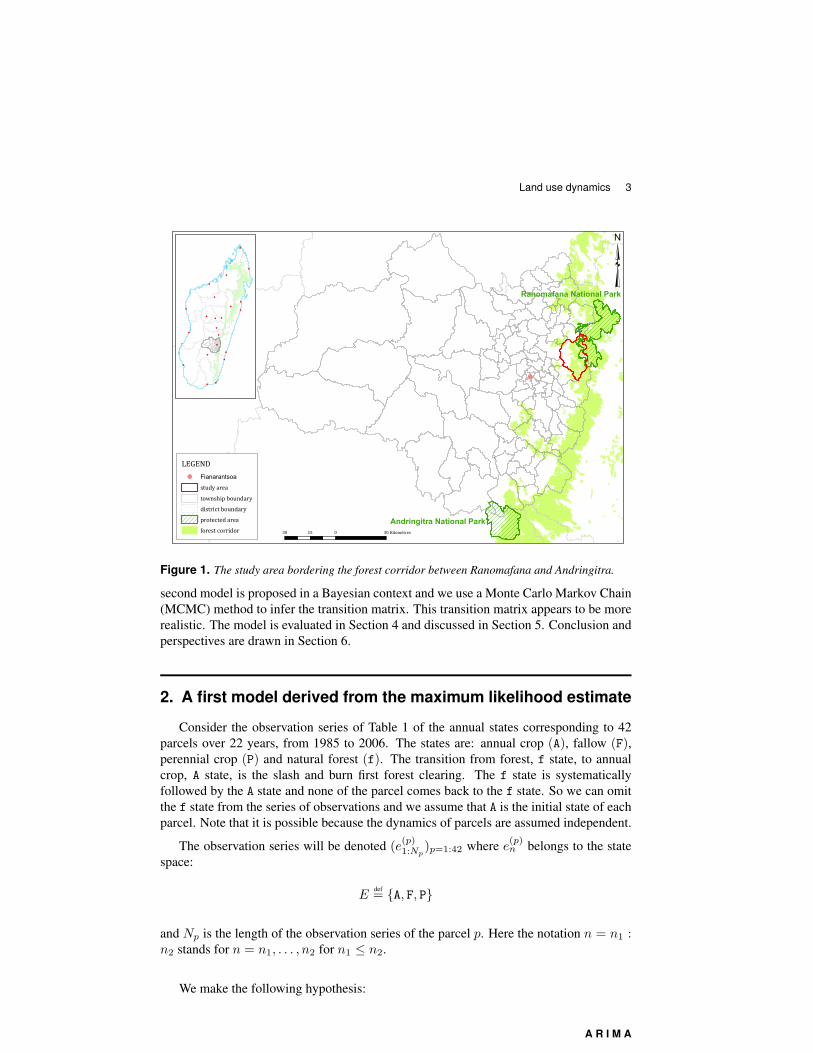
Population pressure is one of the major causes of deforestation in tropical countries. Inthe region of Fianarantsoa (Madagascar), two national parks Ranomafana and Andringitraare connected by a forest corridor, which is of critical importance in maintaining theregional biodiversity [1, 2, 5], see Figure 1. The need for cultivated land pushes peopleto encroach on the corridor to look for lowlands to be converted into paddy fields, andthen to clear slope forested parcels for cultivation. Once lowlands are all converted inpaddy fields, the dynamic of slash and burn cultivation is clearly opposed to the dynamicof forest conservation and regeneration. To reconcile forest conservation with agriculturalproduction, it is important to understand and model the dynamic of post-forest land useof these parcels.

This specific region of Madagascar has already motivated studies in terms of mod-eling. Notably, [1, 2] propose a hierarchical Bayesian model that relates demographicdata with satellite images in order to analyze the links between population pressure anddeforestation at the regional scale.

In contrast to previous models, we will work at the smaller scale of the townshipwith a land-use data set of 42 plots over 22 years; and our model will not capture spatialdependencies. Indeed, the first treatment performed on such a dataset is to build theempirical transition matrix, which is equivalent to assume first that the dynamics of theplots are independent and second that the plot follows an homogeneous Markov dynamicof order 1. We will adopt this simple Markov framework and in this preliminary workwe aim at inferring the time scale at which the dynamics of the agricultural producersstabilizes.

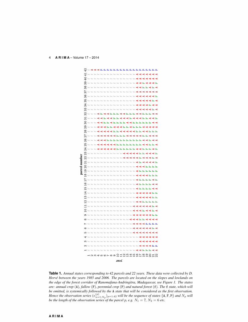
We will use a data set developed by IRD, at the western edge of the corridor, consistingof yearly transitions of 42 parcels initially in forest, these parcels have been cleared since.This set of data is presented in Table 1. Each parcel can take three possible states: annualcrop (A), fallow (F), perennial crop (P).

The use of Markovian approaches to model land-use transitions and vegetation suc-cessions is widespread [19, 20, 22]. The success of these approaches is explained by thefact that agro-ecological dynamics may be represented as discrete-time successions on afinite number of states, each one with its sojourn time. Both agronomists and ecologists,in dialog, actually fail in predicting the future succession of these states, knowing theprevious land-use history. They ask the mathematicians for detailing the characteristicsof these dynamics and defining how to pilot them. The construction, manipulation andsimulation of such models are fairly easy. The transition probabilities of the Markovianmodel are estimated from observed data. The classical reference [3] proposes the max-imum likelihood method to estimate the transition probabilities of a Markov chain. Analternative is to consider Bayesian estimators [18, 13]. In this paper we explore and testseveral modeling tools, Markov chain, Bayesian estimation and MCMC procedure in or-der to find a better fit with the data. These results can then be utilized by agro-ecologiststo model land-use dynamics at a parcel scale.

In Section 2, a first model is directly derived from the data with the help of the empir-ical transition matrix which also corresponds to the maximum likelihood estimate. Thisfirst model is not entirely satisfactory as one of the states is absorbing and does not cor-respond to current knowledge gained by agronomists in the field. Hence, in Section 3, a

A R I M A

Land use dynamics 3

!

!

!

!

!

!

!

!

!

!

!

!

!

!

!

!

!

!

!

!

!

!

Ranomafana National Park

Andringitra National Park

LEGEND! Fianarantsoa

study areatownship boundarydistrict boundaryprotected areaforest corridor 30 0 3015 Kilomètres

³!

!

!

!

!

!

!

!!

!

!!

!

!

!

!

!

!

!

!

!

!

Figure 1. The study area bordering the forest corridor between Ranomafana and Andringitra.

second model is proposed in a Bayesian context and we use a Monte Carlo Markov Chain(MCMC) method to infer the transition matrix. This transition matrix appears to be morerealistic. The model is evaluated in Section 4 and discussed in Section 5. Conclusion andperspectives are drawn in Section 6.

2. A first model derived from the maximum likelihood estimate

Consider the observation series of Table 1 of the annual states corresponding to 42parcels over 22 years, from 1985 to 2006. The states are: annual crop (A), fallow (F),perennial crop (P) and natural forest (f). The transition from forest, f state, to annualcrop, A state, is the slash and burn first forest clearing. The f state is systematicallyfollowed by the A state and none of the parcel comes back to the f state. So we can omitthe f state from the series of observations and we assume that A is the initial state of eachparcel. Note that it is possible because the dynamics of parcels are assumed independent.

The observation series will be denoted (e(p)1:Np

)p=1:42 where e(p)n belongs to the state

space:

Edef= {A, F, P}

and Np is the length of the observation series of the parcel p. Here the notation n = n1 :n2 stands for n = n1, . . . , n2 for n1 ≤ n2.

We make the following hypothesis:

A R I M A

4 A R I M A – Volume 17 – 2014

parc

elnu

mbe

r

year

12

34

56

78

910

1112

1314

1516

1718

1920

2122

2324

2526

2728

2930

3132

3334

3536

3738

3940

4142

1f

ff

ff

ff

ff

ff

ff

ff

ff

ff

ff

ff

ff

ff

ff

ff

ff

ff

ff

ff

ff

f2

ff

ff

ff

ff

ff

ff

ff

ff

ff

ff

ff

ff

ff

ff

ff

ff

ff

ff

ff

ff

fA

3f

ff

ff

ff

ff

ff

ff

ff

ff

ff

ff

ff

ff

ff

ff

ff

ff

ff

ff

ff

ff

A4

ff

ff

ff

ff

ff

ff

ff

ff

ff

ff

ff

fA

AA

AA

AA

AA

ff

ff

ff

ff

fA

5f

ff

ff

ff

ff

ff

ff

ff

ff

ff

ff

ff

AA

AA

AA

AA

Ff

ff

ff

ff

ff

P6

ff

ff

ff

ff

ff

ff

ff

ff

ff

ff

ff

fA

AA

AA

AF

FA

ff

ff

ff

ff

fP

7f

ff

ff

ff

ff

ff

ff

ff

ff

ff

ff

ff

AA

FA

AF

FA

Af

ff

ff

ff

ff

P8

ff

ff

ff

ff

ff

ff

ff

ff

ff

ff

ff

fA

AF

AA

FA

AF

ff

ff

ff

ff

fP

9f

ff

ff

ff

ff

ff

ff

ff

ff

ff

ff

ff

AA

FA

FA

FF

Ff

ff

ff

ff

ff

P10

ff

ff

ff

ff

ff

ff

ff

ff

ff

ff

ff

fF

FF

FF

AF

FF

ff

ff

ff

ff

fP

11f

ff

ff

ff

ff

ff

ff

ff

ff

ff

ff

ff

FF

FF

AA

FA

Af

ff

ff

ff

ff

P12

ff

ff

ff

ff

ff

ff

ff

ff

ff

ff

fA

AF

FF

FA

FF

AA

ff

ff

ff

ff

fP

13f

ff

ff

ff

ff

ff

ff

ff

ff

ff

ff

AA

FF

FA

AF

AA

Ff

ff

ff

ff

ff

P14

ff

ff

ff

fA

ff

ff

ff

ff

ff

ff

fA

AF

FF

AA

AA

FF

ff

ff

ff

ff

fP

15f

ff

fA

AA

AA

AA

ff

ff

ff

ff

ff

AA

FF

FA

AF

FA

Ff

ff

ff

ff

ff

P16

Af

ff

AA

AA

AA

AA

AA

AA

AA

AA

AA

AA

FF

AF

FF

AA

AA

AA

AA

AA

AP

17A

AA

AA

AA

FA

AA

AA

AF

FF

AF

AF

FF

AF

FA

FF

FA

AA

AA

AA

AA

AA

P18

FA

AA

AA

AF

AF

AF

AA

FF

FA

FA

AA

FF

AA

FA

AF

FF

AA

AA

AF

FA

AP

19F

AA

AA

AP

AA

AA

FA

AF

FF

AF

FA

AA

FA

AF

AA

FF

FA

AA

AA

FA

AA

P20

FA

AA

AA

PA

AA

AF

AA

FF

FF

FF

AA

AF

FF

AF

AF

AF

AF

AA

AA

AA

AP

21A

PA

AA

FP

AF

FF

FF

FA

AA

FF

FA

FA

AF

AA

FA

AA

AF

AF

AA

FA

AA

P22

AP

AA

AA

PA

FA

AF

FF

AA

FF

FF

FA

FF

AA

AF

AA

FA

AA

AF

AA

FA

AP

Table 1. Annual states corresponding to 42 parcels and 22 years. These data were collected by D.Hervé between the years 1985 and 2006. The parcels are located on the slopes and lowlands onthe edge of the forest corridor of Ranomafana-Andringitra, Madagascar, see Figure 1. The statesare: annual crop (A), fallow (F), perennial crop (P) and natural forest (f). The f state, which willbe omitted, is systemically followed by the A state that will be considered as the first observation.Hence the observation series (e(p)n=1:Np

)p=1:42 will be the sequence of states {A, F, P} and Np willbe the length of the observation series of the parcel p, e.g. N1 = 7, N2 = 6 etc.

A R I M A

Land use dynamics 5

(H1)The dynamics of the parcels are independent and identical, they are Markovianand time-homogeneous.

This means that (e(p)1:Np

)p=1:42, are 42 independent realizations of a same process (Xn)n≥0

and that this process is Markovian and time-homogeneous.

This assumption is of course simplistic as the dynamics of a given parcel may dependon: farmer decisions; exposition, slope and distance from the forest; neighboring parcels.Assumption (H1) is rather restrictive and unrealistic, nevertheless in the present contextit permits us to infer some interesting results.

This hypothesis leads to a model X = (X(p)1:Np

)p=1:P , where (X(p)n )n=1:Np are P

independent Markov chains, with initial law δA and transition matrix Q of size 3× 3:

P(X(p)1:Np

= e(p)1:Np

, ∀p = 1, . . . , P ) =

P∏

p=1

P(X(p)1:Np

= e1:Np)

=

P∏

p=1

δA (e(p)0 ) Q(e

(p)0 , e

(p)1 ) · · ·Q(e

(p)N−2, e

(p)N−1) (1)

for all e(p)n ∈ E, where Q = [Q(e, e′)]e,e′∈{A,F,P}.

2.1. Maximum likelihood estimate

We derive the maximum likelihood estimate of the transition matrix:

Q = [Q(i, j)]i,j∈E =

1− θ1 − θ2 θ1 θ2

θ3 1− θ3 − θ4 θ4

θ5 θ6 1− θ5 − θ6

(2)

where θ = (θi)1≤i≤6 ∈ Θ with Θdef={θ ∈ [0, 1]6 ; θ1 +θ2 ≤ 1, θ3 +θ4 ≤ 1, θ5 +θ6 ≤

1}

. Let Pθ denote the probability under which the Markov chain admit Q with parameterθ as a transition matrix. We applied the classical results of [3] to compute the MLE ofthe matrix Q. We consider the likelihood function L(θ|(e(p)

1:Np)p=1:P ) of θ given the data

(e(p)1:Np

)p=1:P , for the sake of simplicity we denote it L1(θ), hence:

L1(θ)def= Pθ(X(p)

1:Np= e

(p)1:Np

, ∀p = 1, . . . , P )

=

P∏

p=1

δA (e(p)1 ) Q(e

(p)1 , e

(p)2 ) · · ·Q(e

(p)Np−1, e

(p)Np

)

for any (e(p)1:Np

)p=1:P ∈ E =∏Pp=1E

Np . Let n(p)ee′ be the number of transitions from state

e to state e′ for a parcel p in X:

n(p)ee′

def=

N−1∑

n=1

1{X(p)n−1=e} 1{X(p)

n =e′} ∀e, e′ ∈ E (3)

A R I M A

6 A R I M A – Volume 17 – 2014

and nee′ be the total of number of transitions from state e to state e′ (e, e′ ∈ E):

nee′def=

P∑

p=1

n(p)ee′ . (4)

According to (2) and (4):

L1(θ) =

P∏

p=1

{Q(1, 1)n

(p)AA Q(1, 2)n

(p)AF Q(1, 3)n

(p)AP Q(2, 1)n

(p)FA Q(2, 2)n

(p)FF Q(2, 3)n

(p)FP

Q(3, 1)n(p)PA Q(3, 2)n

(p)PF Q(3, 3)n

(p)PP

}

=

P∏

p=1

{(1− θ1 − θ2)n

(p)AA θ

n(p)AF

1 θn(p)AP

2 θn(p)FA

3 (1− θ3 − θ4)n(p)FF θ

n(p)FP

4

θn(p)PA

5 θn(p)PF

6 (1− θ5 − θ6)n(p)PP

}

= (1− θ1 − θ2)nAA θnAF

1 θnAP

2 θnFA

3 (1− θ3 − θ4)nFF θnFP

4 θnPA

5 θnPF

6 (1− θ5 − θ6)nPP

so that the log-likelihood function is:

l1(θ) = nAA log(1− θ1 − θ2) + nAF log(θ1) + nAP log(θ2)

+ nFA log(θ3) + nFF log(1− θ3 − θ4) + nFP log(θ4)

+ nPA log(θ5) + nPF log(θ6) + nPP log(1− θ5 − θ6) . (5)

The MLE θ is solution of ∂l1(θ)/∂θ|θ=θ = 0, that leads to:

θ1 = nAF/(nAA + nAF + nAP) , θ2 = nAP/(nAA + nAF + nAP) ,

θ3 = nFA/(nFA + nFF + nFP) , θ4 = nFP/(nFA + nFF + nFP) ,

θ5 = nPA/(nPA + nPF + nPP) , θ6 = nPF/(nPA + nPF + nPP) .

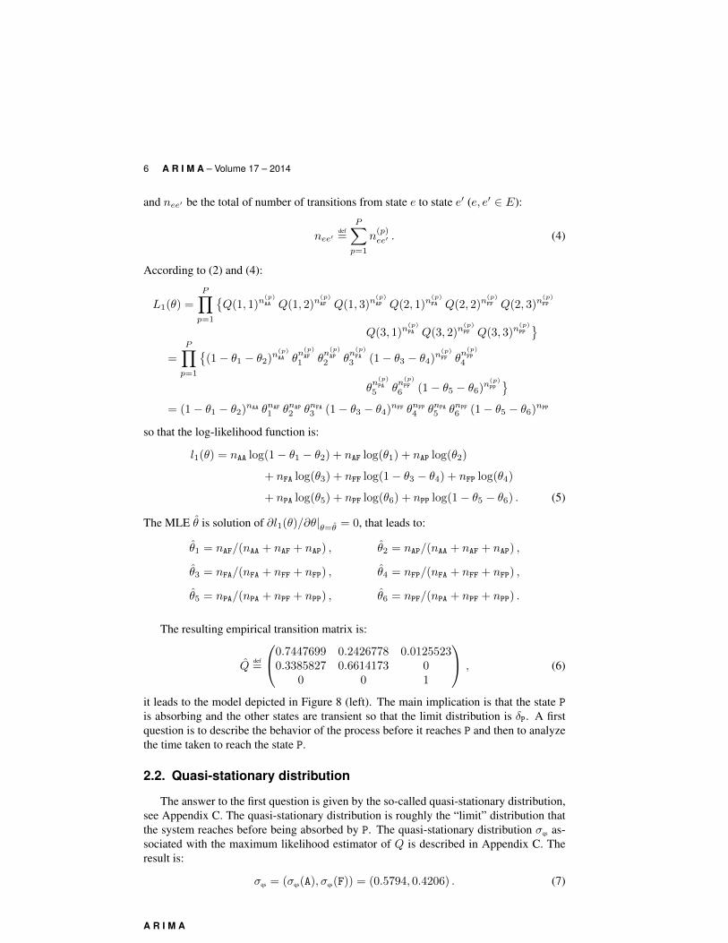
The resulting empirical transition matrix is:

Qdef=

0.7447699 0.2426778 0.01255230.3385827 0.6614173 0

0 0 1

, (6)

it leads to the model depicted in Figure 8 (left). The main implication is that the state Pis absorbing and the other states are transient so that the limit distribution is δP. A firstquestion is to describe the behavior of the process before it reaches P and then to analyzethe time taken to reach the state P.

2.2. Quasi-stationary distribution

The answer to the first question is given by the so-called quasi-stationary distribution,see Appendix C. The quasi-stationary distribution is roughly the “limit” distribution thatthe system reaches before being absorbed by P. The quasi-stationary distribution σqs as-sociated with the maximum likelihood estimator of Q is described in Appendix C. Theresult is:

σqs = (σqs(A), σqs(F)) = (0.5794, 0.4206) . (7)

A R I M A

Land use dynamics 7

Hence, conditionally on the fact that the process does not reach P, it will spend 58% of itstime in the A state and 42% of its time in the F state.

2.3. Distribution of the time to reach P

50 100 150 200 250 3000

0.005

0.01

0.015

time n

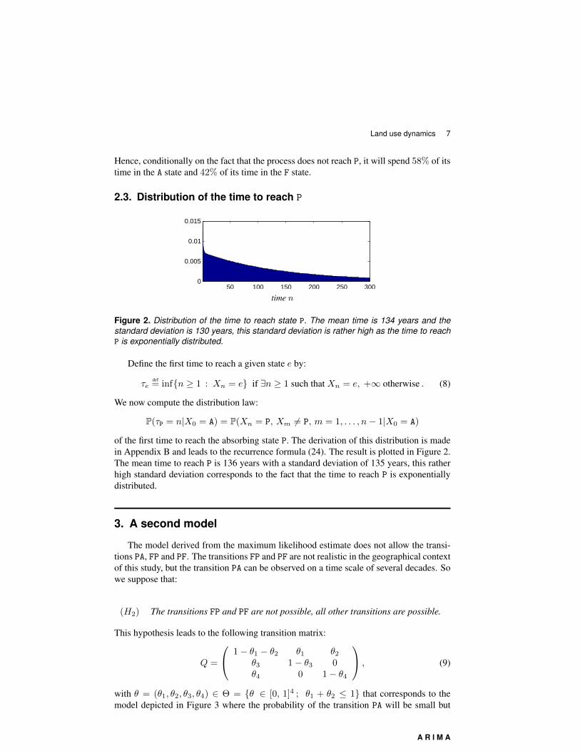
Figure 2. Distribution of the time to reach state P. The mean time is 134 years and thestandard deviation is 130 years, this standard deviation is rather high as the time to reachP is exponentially distributed.

Define the first time to reach a given state e by:

τedef= inf{n ≥ 1 : Xn = e} if ∃n ≥ 1 such that Xn = e, +∞ otherwise . (8)

We now compute the distribution law:

P(τP = n|X0 = A) = P(Xn = P, Xm 6= P, m = 1, . . . , n− 1|X0 = A)

of the first time to reach the absorbing state P. The derivation of this distribution is madein Appendix B and leads to the recurrence formula (24). The result is plotted in Figure 2.The mean time to reach P is 136 years with a standard deviation of 135 years, this ratherhigh standard deviation corresponds to the fact that the time to reach P is exponentiallydistributed.

3. A second model

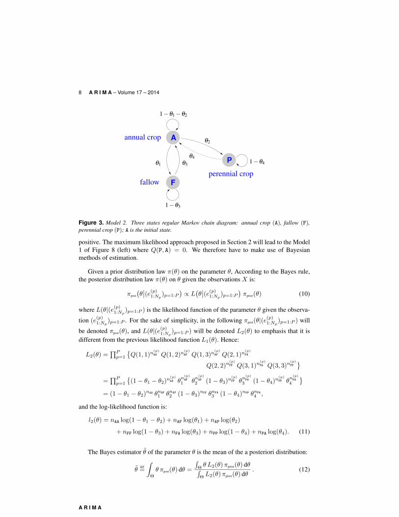
The model derived from the maximum likelihood estimate does not allow the transi-tions PA, FP and PF. The transitions FP and PF are not realistic in the geographical contextof this study, but the transition PA can be observed on a time scale of several decades. Sowe suppose that:

(H2) The transitions FP and PF are not possible, all other transitions are possible.

This hypothesis leads to the following transition matrix:

Q =

1− θ1 − θ2 θ1 θ2

θ3 1− θ3 0θ4 0 1− θ4

, (9)

with θ = (θ1, θ2, θ3, θ4) ∈ Θ = {θ ∈ [0, 1]4 ; θ1 + θ2 ≤ 1} that corresponds to themodel depicted in Figure 3 where the probability of the transition PA will be small but

A R I M A

8 A R I M A – Volume 17 – 2014

8 A. RAHERINIRINA, D. HERVE, R. RAKOTOZAFY AND F. CAMPILLO

50 100 150 200 250 3000

0.005

0.01

0.015

time n

Figure 2. Distribution of the time to reach state P. The mean time is 134 years and thestandard deviation is 130 years, this standard deviation is rather high as the time to reachP is exponentially distributed.

F

P

A q2

1�q1�q2

1�q3

fallowperennial crop

1�q4q1 q3

q4

annual crop

Figure 3. Model 2. Three states regular Markov chain diagram: annual crop (A), fallow(F), perennial crop (P); A is the initial state.

3 A SECOND MODELThe model derived from the maximum likelihood estimate does not allow the

transitions PA, FP and PF. The transitions FP and PF are not realistic in the geo-graphical context of this study, but the transition PA can be observed on a time scaleof several decades. So we suppose that:

(H2)The transitions FP and PF are not possible, all other transitions arepossible.

This hypothesis leads to the following transition matrix:

Q =

0B@

1�q1�q2 q1 q2

q3 1�q3 0q4 0 1�q4

1CA , (3.1)

with q = (q1,q2,q3,q4) 2 Q = {q 2 [0, 1]4 ; q1 + q2 1} that corresponds to themodel depicted in Figure ?? where the probability of the transition PA will be smallbut positive. The maximum likelihood approach proposed in Section 2 will lead to

Figure 3. Model 2. Three states regular Markov chain diagram: annual crop (A), fallow (F),perennial crop (P); A is the initial state.

positive. The maximum likelihood approach proposed in Section 2 will lead to the Model1 of Figure 8 (left) where Q(P, A) = 0. We therefore have to make use of Bayesianmethods of estimation.

Given a prior distribution law π(θ) on the parameter θ, According to the Bayes rule,the posterior distribution law π(θ) on θ given the observations X is:

πpost

(θ∣∣(e(p)

1:Np)p=1:P

)∝ L

(θ∣∣(e(p)

1:Np)p=1:P

)πprior(θ) (10)

where L(θ|(e(p)1:Np

)p=1:P ) is the likelihood function of the parameter θ given the observa-

tion (e(p)1:Np

)p=1:P . For the sake of simplicity, in the following πpost(θ|(e(p)1:Np

)p=1:P ) will

be denoted πpost(θ), and L(θ|(e(p)1:Np

)p=1:P ) will be denoted L2(θ) to emphasis that it isdifferent from the previous likelihood function L1(θ). Hence:

L2(θ) =∏Pp=1

{Q(1, 1)n

(p)AA Q(1, 2)n

(p)AF Q(1, 3)n

(p)AP Q(2, 1)n

(p)FA

Q(2, 2)n(p)FF Q(3, 1)n

(p)PA Q(3, 3)n

(p)PP

}

=∏Pp=1

{(1− θ1 − θ2)n

(p)AA θ

n(p)AF

1 θn(p)AP

2 (1− θ3)n(p)FF θ

n(p)FA

3 (1− θ4)n(p)PP θ

n(p)PA

4

}

= (1− θ1 − θ2)nAA θnAF

1 θnAP

2 (1− θ3)nFF θnFA

3 (1− θ4)nPP θnPA

4 ,

and the log-likelihood function is:

l2(θ) = nAA log(1− θ1 − θ2) + nAF log(θ1) + nAP log(θ2)

+ nFF log(1− θ3) + nFA log(θ3) + nPP log(1− θ4) + nPA log(θ4). (11)

The Bayes estimator θ of the parameter θ is the mean of the a posteriori distribution:

θdef=

∫

Θ

θ πpost(θ) dθ =

∫Θθ L2(θ)πprior(θ) dθ∫

ΘL2(θ)πprior(θ) dθ

. (12)

A R I M A

Land use dynamics 9

3.1. Jeffreys prior

Numerical tests that will be performed in Section 3.2.1 suggest that the Jeffreys prior iswell adapted to the present situation. This prior distribution (non-informative) is definedby [12]:

πprior(θ) ∝√

det[I(θ)] (13)

where I(θ) is the Fisher information matrix given by:

I(θ)def=

[Eθ(− ∂2l2(θ)

∂θk ∂θl

)]

1≤k,l≤4

and l2(θ) is the log-likelihood function (11). Hence:

I(θ) =

A1,2 0 00 a3 00 0 a4

with

Ak,`def= −Eθ

(∂2l2(θ)∂2θk

∂2l2(θ)∂θk∂θ`

∂2l2(θ)∂θk∂θ`

∂2l2(θ)∂2θ`

), ak

def= −Eθ

(∂2l2(θ)

∂2θk

).

So det I(θ) = detA1,2 × a3 × a4 and

πprior(θ) ∝√

detA1,2 × a3 × a4 . (14a)

According to (11):

∂2l2(θ)

∂2θ1= −

(nAA

(1− θ1 − θ2)2+nAFθ2

1

),

∂2l2(θ)

∂θ1 ∂θ2= − nAA

(1− θ1 − θ2)2,

∂2l2(θ)

∂2θ2= −

(nAA

(1− θ1 − θ2)2+nAPθ2

2

),

∂2l2(θ)

∂θ2 ∂θ1= − nAA

(1− θ1 − θ2)2, ,

∂2l2(θ)

∂2θ3= −

(nFF

(1− θ3)2+nFAθ2

3

),

∂2l2(θ)

∂2θ4= −

(nPP

(1− θ4)2+nPAθ2

4

)

and

detA1,2 =(

Eθ[nAA](1−θ1−θ2)2 + Eθ[nAF]

θ21

) (Eθ[nAA]

(1−θ1−θ2)2 + Eθ[nAP]θ22

)−(

Eθ[nAA](1−θ1−θ2)2

)2

, (14b)

a3 = Eθ[nFF](1−θ3)2 + Eθ[nFA]

θ23, (14c)

a4 = Eθ[nPP](1−θ4)2 + Eθ[nPA]

θ24. (14d)

A R I M A

10 A R I M A – Volume 17 – 2014

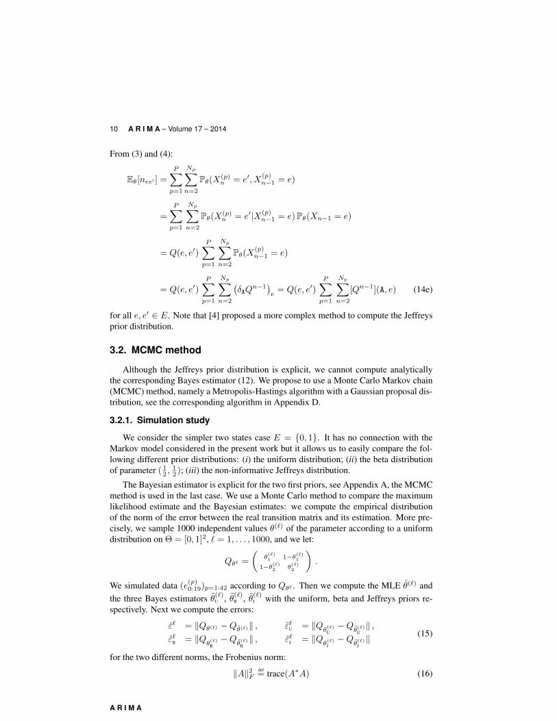
From (3) and (4):

Eθ[nee′ ] =

P∑

p=1

Np∑

n=2

Pθ(X(p)n = e′, X

(p)n−1 = e)

=

P∑

p=1

Np∑

n=2

Pθ(X(p)n = e′|X(p)

n−1 = e)Pθ(Xn−1 = e)

= Q(e, e′)

P∑

p=1

Np∑

n=2

Pθ(X(p)n−1 = e)

= Q(e, e′)

P∑

p=1

Np∑

n=2

(δAQ

n−1)e

= Q(e, e′)

P∑

p=1

Np∑

n=2

[Qn−1](A, e) (14e)

for all e, e′ ∈ E. Note that [4] proposed a more complex method to compute the Jeffreysprior distribution.

3.2. MCMC method

Although the Jeffreys prior distribution is explicit, we cannot compute analyticallythe corresponding Bayes estimator (12). We propose to use a Monte Carlo Markov chain(MCMC) method, namely a Metropolis-Hastings algorithm with a Gaussian proposal dis-tribution, see the corresponding algorithm in Appendix D.

3.2.1. Simulation study

We consider the simpler two states case E = {0, 1}. It has no connection with theMarkov model considered in the present work but it allows us to easily compare the fol-lowing different prior distributions: (i) the uniform distribution; (ii) the beta distributionof parameter ( 1

2 ,12 ); (iii) the non-informative Jeffreys distribution.

The Bayesian estimator is explicit for the two first priors, see Appendix A, the MCMCmethod is used in the last case. We use a Monte Carlo method to compare the maximumlikelihood estimate and the Bayesian estimates: we compute the empirical distributionof the norm of the error between the real transition matrix and its estimation. More pre-cisely, we sample 1000 independent values θ(`) of the parameter according to a uniformdistribution on Θ = [0, 1]2, ` = 1, . . . , 1000, and we let:

Qθ` =

(θ(`)1 1−θ(`)1

1−θ(`)2 θ(`)2

).

We simulated data (e(p)0:19)p=1:42 according to Qθ` . Then we compute the MLE θ(`) and

the three Bayes estimators θ(`)U , θ(`)

B , θ(`)J with the uniform, beta and Jeffreys priors re-

spectively. Next we compute the errors:

ε` = ‖Qθ(`) −Qθ(`)‖ , ε`U = ‖Qθ(`)U−Q

θ(`)U‖ ,

ε`B = ‖Qθ(`)B−Q

θ(`)B‖ , ε`J = ‖Q

θ(`)J−Q

θ(`)J‖ (15)

for the two different norms, the Frobenius norm:

‖A‖2Fdef= trace(A∗A) (16)

A R I M A

Land use dynamics 11

Matrix 2−Norm

Errors0.0 0.2 0.4 0.6 0.8 1.0

Bayesian estimate with Jeffrey priormaximum likelihood estimateBayesian estimate with uniform priorBayesian estimate with beta prior

Frobenius Matrix Norm

Errors0.0 0.2 0.4 0.6 0.8 1.0

Bayesian estimate with Jeffrey priormaximum likelihood estimateBayesian estimate with uniform priorBayesian estimate with beta prior

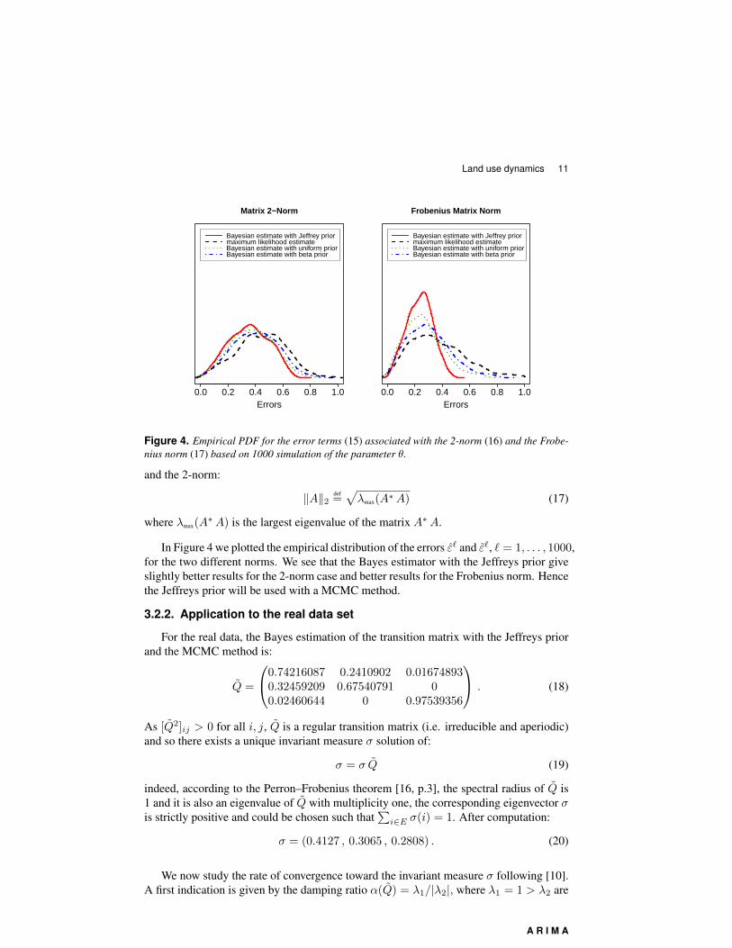
Figure 4. Empirical PDF for the error terms (15) associated with the 2-norm (16) and the Frobe-nius norm (17) based on 1000 simulation of the parameter θ.

and the 2-norm:

‖A‖2 def=√λmax(A∗A) (17)

where λmax(A∗A) is the largest eigenvalue of the matrix A∗A.

In Figure 4 we plotted the empirical distribution of the errors ε` and ε`, ` = 1, . . . , 1000,for the two different norms. We see that the Bayes estimator with the Jeffreys prior giveslightly better results for the 2-norm case and better results for the Frobenius norm. Hencethe Jeffreys prior will be used with a MCMC method.

3.2.2. Application to the real data set

For the real data, the Bayes estimation of the transition matrix with the Jeffreys priorand the MCMC method is:

Q =

0.74216087 0.2410902 0.016748930.32459209 0.67540791 00.02460644 0 0.97539356

. (18)

As [Q2]ij > 0 for all i, j, Q is a regular transition matrix (i.e. irreducible and aperiodic)and so there exists a unique invariant measure σ solution of:

σ = σ Q (19)

indeed, according to the Perron–Frobenius theorem [16, p.3], the spectral radius of Q is1 and it is also an eigenvalue of Q with multiplicity one, the corresponding eigenvector σis strictly positive and could be chosen such that

∑i∈E σ(i) = 1. After computation:

σ = (0.4127 , 0.3065 , 0.2808) . (20)

We now study the rate of convergence toward the invariant measure σ following [10].A first indication is given by the damping ratio α(Q) = λ1/|λ2|, where λ1 = 1 > λ2 are

A R I M A

12 A R I M A – Volume 17 – 2014

12 A. RAHERINIRINA, D. HERVE, R. RAKOTOZAFY AND F. CAMPILLO

Matrix 2−Norm

Errors0.0 0.2 0.4 0.6 0.8 1.0

Bayesian estimate with Jeffrey priormaximum likelihood estimateBayesian estimate with uniform priorBayesian estimate with beta prior

Frobenius Matrix Norm

Errors0.0 0.2 0.4 0.6 0.8 1.0

Bayesian estimate with Jeffrey priormaximum likelihood estimateBayesian estimate with uniform priorBayesian estimate with beta prior

Figure 4. Empirical PDF for the error terms (3.7) associated with the 2-norm (3.8) and theFrobenius norm (3.9) based on 1000 simulation of the parameter q .

θ1

MC

MC

iter

atio

n0

40000

80000

0.1 0.2 0.3 0.4

ech_1[P1]

θ2M

CM

C it

erat

ion

040000

80000

0.00 0.02 0.04 0.06

ech_2[P2]

θ3

MC

MC

iter

atio

n0

40000

80000

0.2 0.3 0.4 0.5

ech_3[P3]

θ4

MC

MC

iter

atio

n0

40000

80000

0.00 0.05 0.10 0.15

ech_4

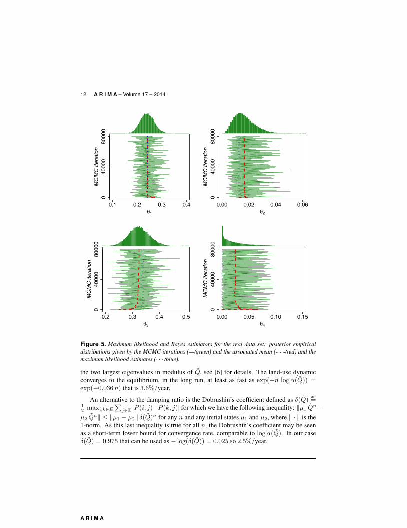
Figure 5. Maximum likelihood and Bayes estimators for the real data set: posterior em-pirical distributions given by the MCMC iterations (—/green) and the associated mean (- --/red) and the maximum likelihood estimates (· · · /blue).

Figure 5. Maximum likelihood and Bayes estimators for the real data set: posterior empiricaldistributions given by the MCMC iterations (—/green) and the associated mean (- - -/red) and themaximum likelihood estimates (· · · /blue).

the two largest eigenvalues in modulus of Q, see [6] for details. The land-use dynamicconverges to the equilibrium, in the long run, at least as fast as exp(−n logα(Q)) =exp(−0.036n) that is 3.6%/year.

An alternative to the damping ratio is the Dobrushin’s coefficient defined as δ(Q)def=

12 maxi,k∈E

∑j∈E |P (i, j)−P (k, j)| for which we have the following inequality: ‖µ1 Q

n−µ2 Q

n‖ ≤ ‖µ1 − µ2‖ δ(Q)n for any n and any initial states µ1 and µ2, where ‖ · ‖ is the1-norm. As this last inequality is true for all n, the Dobrushin’s coefficient may be seenas a short-term lower bound for convergence rate, comparable to logα(Q). In our caseδ(Q) = 0.975 that can be used as − log(δ(Q)) = 0.025 so 2.5%/year.

A R I M A

Land use dynamics 13

4. Model evaluation

4.1. Sojourn time test

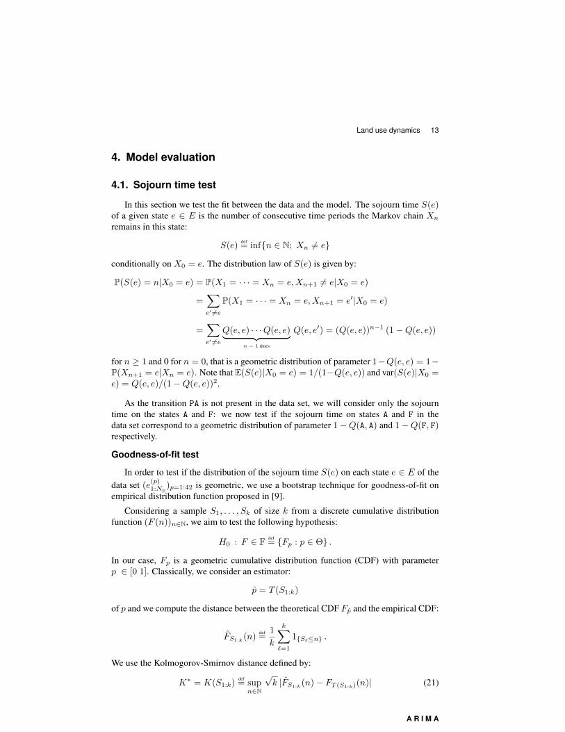
In this section we test the fit between the data and the model. The sojourn time S(e)of a given state e ∈ E is the number of consecutive time periods the Markov chain Xn

remains in this state:

S(e)def= inf{n ∈ N; Xn 6= e}

conditionally on X0 = e. The distribution law of S(e) is given by:

P(S(e) = n|X0 = e) = P(X1 = · · · = Xn = e,Xn+1 6= e|X0 = e)

=∑

e′ 6=e

P(X1 = · · · = Xn = e,Xn+1 = e′|X0 = e)

=∑

e′ 6=e

Q(e, e) · · ·Q(e, e)︸ ︷︷ ︸n − 1 times

Q(e, e′) = (Q(e, e))n−1 (1−Q(e, e))

for n ≥ 1 and 0 for n = 0, that is a geometric distribution of parameter 1−Q(e, e) = 1−P(Xn+1 = e|Xn = e). Note that E(S(e)|X0 = e) = 1/(1−Q(e, e)) and var(S(e)|X0 =e) = Q(e, e)/(1−Q(e, e))2.

As the transition PA is not present in the data set, we will consider only the sojourntime on the states A and F: we now test if the sojourn time on states A and F in thedata set correspond to a geometric distribution of parameter 1−Q(A, A) and 1−Q(F, F)respectively.

Goodness-of-fit test

In order to test if the distribution of the sojourn time S(e) on each state e ∈ E of thedata set (e

(p)1:Np

)p=1:42 is geometric, we use a bootstrap technique for goodness-of-fit onempirical distribution function proposed in [9].

Considering a sample S1, . . . , Sk of size k from a discrete cumulative distributionfunction (F (n))n∈N, we aim to test the following hypothesis:

H0 : F ∈ F def= {Fp : p ∈ Θ} .

In our case, Fp is a geometric cumulative distribution function (CDF) with parameterp ∈ [0 1]. Classically, we consider an estimator:

p = T (S1:k)

of p and we compute the distance between the theoretical CDF Fp and the empirical CDF:

FS1:k(n)

def=

1

k

k∑

`=1

1{S`≤n} .

We use the Kolmogorov-Smirnov distance defined by:

K∗ = K(S1:k)def= supn∈N

√k |FS1:k

(n)− FT (S1:k)(n)| (21)

A R I M A

14 A R I M A – Volume 17 – 2014

A (annual crop) Sojourn time values 1 2 3 4 5 6Number of occurrences 11 17 12 5 9 7

F (fallow) Sojourn time values 1 2 3 4 6 8 11Number of occurrences 16 12 7 4 2 1 1

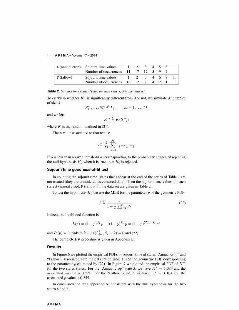
Table 2. Sojourn time values (year) on each state A, F in the data set.

To establish whether K∗ is significantly different from 0 or not, we simulate M samplesof size k:

Sm1 , . . . , Smk

iid∼ Fp, m = 1, . . . ,M

and we let:Km def

= K(Sm1:k)

where K is the function defined in (21).

The p-value associated to that test is:

ρdef=

1

M

M∑

m=1

1{Km≥K∗} .

If ρ is less than a given threshold α, corresponding to the probability chance of rejectingthe null hypothesis H0 when it is true, then H0 is rejected.

Sojourn time goodness-of-fit test

In counting the sojourn time, states that appear at the end of the series of Table 1 arenot treated (they are considered as censored data). Then the sojourn time values on eachstate A (annual crop), F (fallow) in the data set are given in Table 2.

To test the hypothesis H0 we use the MLE for the parameter p of the geometric PDF:

pdef=

1

1 + 1k

∑k`=1 S`

. (22)

Indeed, the likelihood function is:

L(p) = (1− p)S1 p · · · (1− p)Sk p = (1− p)∑k`=1 S` pk

and L′(p) = 0 leads to k − p (∑k`=1 S` + k) = 0 and (22).

The complete test procedure is given in Appendix E.

Results

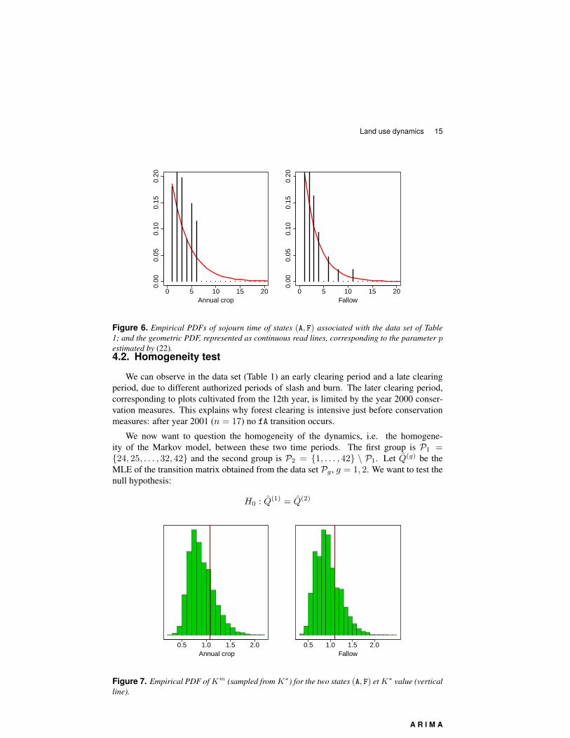
In Figure 6 we plotted the empirical PDFs of sojourn time of states “Annual crop” and“Fallow”, associated with the data set of Table 1, and the geometric PDF correspondingto the parameter p estimated by (22). In Figure 7 we plotted the empirical PDF of Km

for the two states states. For the “Annual crop” state A, we have K∗ = 1.086 and theassociated p-value is 0.224. For the “Fallow” state F, we have K∗ = 1.104 and theassociated p-value is 0.255.

In conclusion the data appear to be consistent with the null hypothesis for the twostates A and F.

A R I M A

Land use dynamics 15

Annual crop 0 5 10 15 20

0.00

0.05

0.10

0.15

0.20

Fallow0 5 10 15 20

0.00

0.05

0.10

0.15

0.20

Figure 6. Empirical PDFs of sojourn time of states (A, F) associated with the data set of Table1; and the geometric PDF, represented as continuous read lines, corresponding to the parameter pestimated by (22).4.2. Homogeneity test

We can observe in the data set (Table 1) an early clearing period and a late clearingperiod, due to different authorized periods of slash and burn. The later clearing period,corresponding to plots cultivated from the 12th year, is limited by the year 2000 conser-vation measures. This explains why forest clearing is intensive just before conservationmeasures: after year 2001 (n = 17) no fA transition occurs.

We now want to question the homogeneity of the dynamics, i.e. the homogene-ity of the Markov model, between these two time periods. The first group is P1 ={24, 25, . . . , 32, 42} and the second group is P2 = {1, . . . , 42} \ P1. Let Q(g) be theMLE of the transition matrix obtained from the data set Pg , g = 1, 2. We want to test thenull hypothesis:

H0 : Q(1) = Q(2)

Annual crop0.5 1.0 1.5 2.0

Fallow0.5 1.0 1.5 2.0

Figure 7. Empirical PDF ofKm (sampled fromK∗) for the two states (A, F) etK∗ value (verticalline).

A R I M A

16 A R I M A – Volume 17 – 201418 A. RAHERINIRINA, D. HERVE, R. RAKOTOZAFY AND F. CAMPILLO

F

P

A

1

fallow

annual crop

perennial crop

0.66

0.74

0.24

0.02

0.34

F

P

A

fallowperennial crop

annual crop

0.98

0.68

0.320.02

0.74

0.24

0.02

Model 1 Model 2Maximum likelihood estimation Bayesian estimation

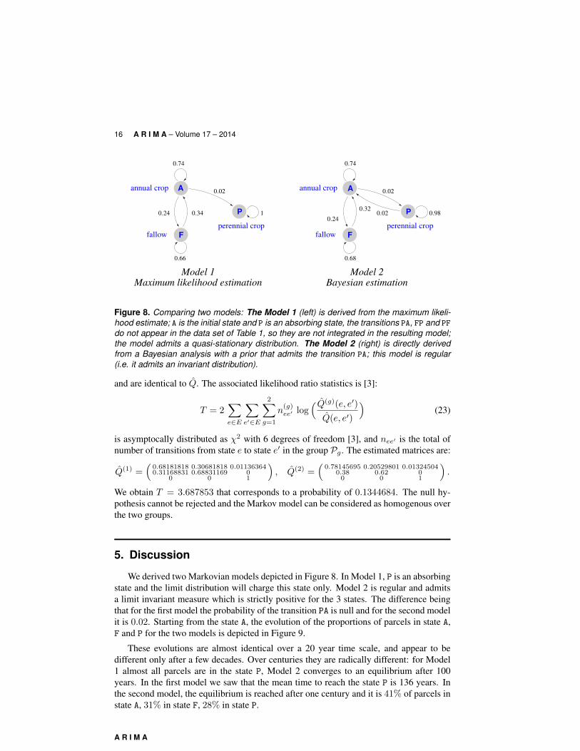
Figure 8. Comparing two models: The Model 1 (left) is derived from the maximum likeli-hood estimate; A is the initial state and P is an absorbing state, the transitions PA, FP andPF do not appear in the data set of Table 1, so they are not integrated in the resulting model;the model admits a quasi-stationary distribution. The Model 2 (right) is directly derivedfrom a Bayesian analysis with a prior that admits the transition PA; this model is regular(i.e. it admits an invariant distribution).

0 200

0.5

1

year

mod

el 1

prop

ortio

ns

0 1000

0.5

1

year

prop

ortio

ns

0 5000

0.5

1

year

prop

ortio

ns

A annual cropF fallowP perennial crop

0 200

0.5

1

year

mod

el 2

prop

ortio

ns

0 1000

0.5

1

year

prop

ortio

ns

0 5000

0.5

1

year

prop

ortio

ns

Figure 9. Evolution of the proportions of parcels in state A, F and P during 20, 100 and 500years according to the Models 1 and 2.

5 DISCUSSIONWe derived two Markovian models depicted in Figure 8. In Model 1, P is an

absorbing state and the limit distribution will charge this state only. Model 2 isregular and admits a limit invariant measure which is strictly positive for the 3 states.The difference being that for the first model the probability of the transition PA isnull and for the second model it is 0.02. Starting from the state A, the evolution ofthe proportions of parcels in state A, F and P for the two models is depicted in Figure9.

These evolutions are almost identical over a 20 year time scale, and appear to bedifferent only after a few decades. Over centuries they are radically different: forModel 1 almost all parcels are in the state P, Model 2 converges to an equilibrium

Figure 8. Comparing two models: The Model 1 (left) is derived from the maximum likeli-hood estimate; A is the initial state and P is an absorbing state, the transitions PA, FP and PF

do not appear in the data set of Table 1, so they are not integrated in the resulting model;the model admits a quasi-stationary distribution. The Model 2 (right) is directly derivedfrom a Bayesian analysis with a prior that admits the transition PA; this model is regular(i.e. it admits an invariant distribution).

and are identical to Q. The associated likelihood ratio statistics is [3]:

T = 2∑

e∈E

∑

e′∈E

2∑

g=1

n(g)ee′ log

( Q(g)(e, e′)

Q(e, e′)

)(23)

is asymptocally distributed as χ2 with 6 degrees of freedom [3], and nee′ is the total ofnumber of transitions from state e to state e′ in the group Pg . The estimated matrices are:

Q(1) =(

0.68181818 0.30681818 0.011363640.31168831 0.68831169 0

0 0 1

), Q(2) =

(0.78145695 0.20529801 0.01324504

0.38 0.62 00 0 1

).

We obtain T = 3.687853 that corresponds to a probability of 0.1344684. The null hy-pothesis cannot be rejected and the Markov model can be considered as homogenous overthe two groups.

5. Discussion

We derived two Markovian models depicted in Figure 8. In Model 1, P is an absorbingstate and the limit distribution will charge this state only. Model 2 is regular and admitsa limit invariant measure which is strictly positive for the 3 states. The difference beingthat for the first model the probability of the transition PA is null and for the second modelit is 0.02. Starting from the state A, the evolution of the proportions of parcels in state A,F and P for the two models is depicted in Figure 9.

These evolutions are almost identical over a 20 year time scale, and appear to bedifferent only after a few decades. Over centuries they are radically different: for Model1 almost all parcels are in the state P, Model 2 converges to an equilibrium after 100years. In the first model we saw that the mean time to reach the state P is 136 years. Inthe second model, the equilibrium is reached after one century and it is 41% of parcels instate A, 31% in state F, 28% in state P.

A R I M A

Land use dynamics 17

0 200

0.5

1

year

mod

el 1

prop

ortio

ns

0 1000

0.5

1

year

prop

ortio

ns

0 5000

0.5

1

year

prop

ortio

ns

A annual cropF fallowP perennial crop

0 200

0.5

1

year

mod

el 2

prop

ortio

ns

0 1000

0.5

1

year

prop

ortio

ns

0 5000

0.5

1

year

prop

ortio

ns

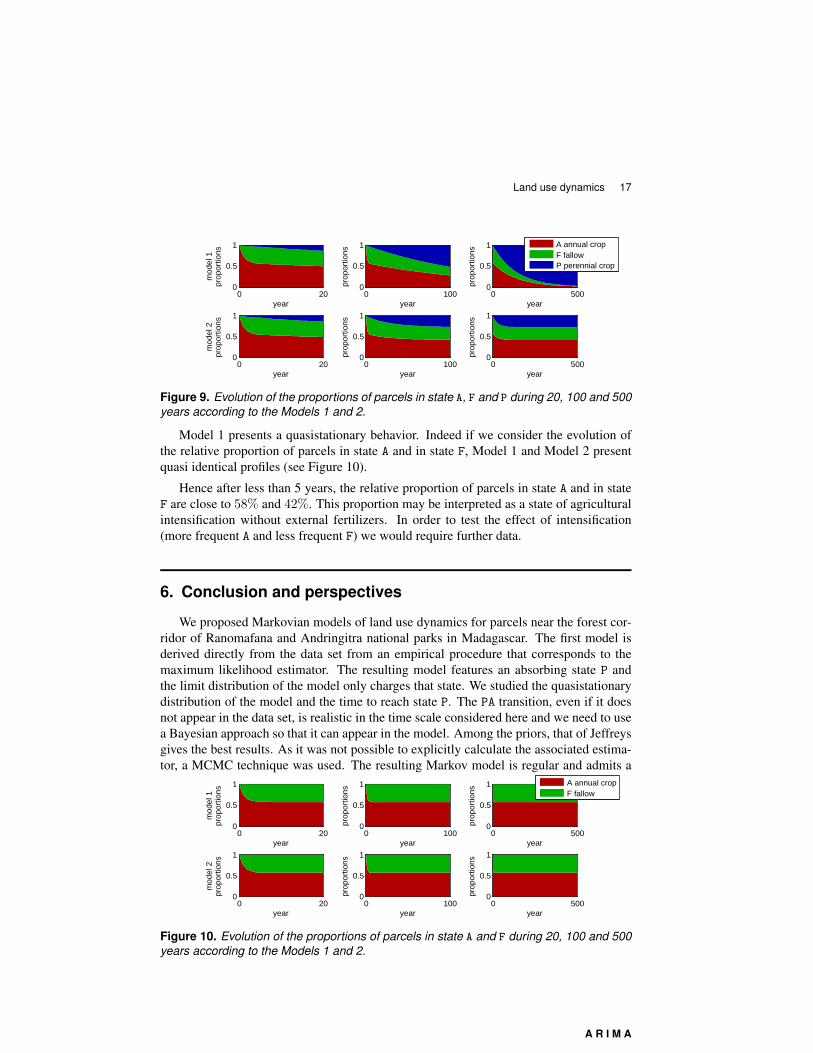
Figure 9. Evolution of the proportions of parcels in state A, F and P during 20, 100 and 500years according to the Models 1 and 2.

Model 1 presents a quasistationary behavior. Indeed if we consider the evolution ofthe relative proportion of parcels in state A and in state F, Model 1 and Model 2 presentquasi identical profiles (see Figure 10).

Hence after less than 5 years, the relative proportion of parcels in state A and in stateF are close to 58% and 42%. This proportion may be interpreted as a state of agriculturalintensification without external fertilizers. In order to test the effect of intensification(more frequent A and less frequent F) we would require further data.

6. Conclusion and perspectives

We proposed Markovian models of land use dynamics for parcels near the forest cor-ridor of Ranomafana and Andringitra national parks in Madagascar. The first model isderived directly from the data set from an empirical procedure that corresponds to themaximum likelihood estimator. The resulting model features an absorbing state P andthe limit distribution of the model only charges that state. We studied the quasistationarydistribution of the model and the time to reach state P. The PA transition, even if it doesnot appear in the data set, is realistic in the time scale considered here and we need to usea Bayesian approach so that it can appear in the model. Among the priors, that of Jeffreysgives the best results. As it was not possible to explicitly calculate the associated estima-tor, a MCMC technique was used. The resulting Markov model is regular and admits a

0 200

0.5

1

year

mod

el 1

prop

ortio

ns

0 1000

0.5

1

year

prop

ortio

ns

0 5000

0.5

1

year

prop

ortio

ns

0 200

0.5

1

year

mod

el 2

prop

ortio

ns

0 1000

0.5

1

year

prop

ortio

ns

0 5000

0.5

1

year

prop

ortio

ns

A annual cropF fallow

Figure 10. Evolution of the proportions of parcels in state A and F during 20, 100 and 500years according to the Models 1 and 2.

A R I M A

18 A R I M A – Volume 17 – 2014

unique invariant measure that charges all the states. We studied the speed of convergenceto this limit distribution.

We assessed the adequacy of the model to real data. We focused on the sojourn times:we tested if the empirical sojourn times correspond to a geometric distribution. We used aparametric bootstrap goodness-of-fit on empirical distribution. We also tested the spatialhomogeneity of the model.

A new database is currently being developed by the IRD. It will cover a longer periodof time and a greater number of parcels, it will also allow us to consider a more detailedstate space comprising more than three states.

Part of the complexity of these agro-ecological temporal data comes from the factthat some transitions are “natural”, due to ecological dynamics, while others come fromhuman decisions (annual cropping, crop abandonment, planting perennial crops, etc.). Itshould also be interesting to study the dynamics of parcels conditionally on the dynamicsof the neighboring parcels. This model could be more realistic but would require a largernumber of unknown parameters that the present data set will not permit to infer and amore in depth study of the farmers’ practices will hence be necessary.

In the case of retrospective studies and forest-agriculture transitions, we lack a longterm series of plot use histories, especially in tropical southern countries. The effect of alimited database, either in size (number of plots) or in time (period), is poorly known. Inthis context, the Bayesian approach is of interest in developing further conclusions basedon complementary knowledge from agronomists, ecologists and geographers.

Acknowledgements

This works was partially supported by the LIRIMA/INRIA program and by the Coop-eration and Cultural Action Office (SCAC) of the France Embassy in Madagascar.

Appendices

A. Explicit Bayes estimators for the two states case

Let (Xn)0≤n≤N be a Markov chain with two states {0, 1} and transition matrix

Qdef=( p 1−p

1−q q

).

We suppose that the initial law is the invariant distribution µ = (q/p+ q, p/p+ q), thatis the solution of µQ = µ. The unknown parameter is θ = (p, q) ∈ [0, 1]2 and theassociated likelihood function is

LN (θ)def= Pθ(X0:N = x0:N ) = (1− p)n00 pn01 qn10 (1− q)n11

where nijdef= nij(x0:N ) =

∑N−1n=0 1{Xn=i} 1{Xn+1=j} is the number of transition i → j

in x0:N .

We consider the following priori distributions: the uniform distribution πU on [0, 1]2

and the beta distribution πB with parameters (a, b), that is

πB(θ) =1

β(a, b)θa−1 (1− θ)b−1

A R I M A

Land use dynamics 19

where β(a, b) is the beta function:

β(a, b)def=

∫ 1

0

xa−1 (1− x)b−1 dx =Γ(a) Γ(b)

Γ(a+ b)

with Γ(z)def=∫ +∞

0tz−1 e−t dt. Here we will choose a = b = 1/2, note that Γ(1) = 1

and Γ( 12 ) =

√π. For these two priors we can explicitly compute the posterior distriution

and the associated Bayes estimators. Indeed the posterior distribution πpost is given by theBayes formula: πpost(θ) ∝ LN (θ)π(θ), that is:

πUpost(θ) ∝ LN (θ) = (1− p)n00 pn01 qn10 (1− q)n11 ,

πBpost(θ) ∝ LN (θ)πB(θ) = (1− p)n00− 1

2 pn01− 12 qn10− 1

2 (1− q)n11− 12

and the corresponding Bayes estimator are:

θU =

∫

[0,1]2θ πU

post(θ) dθ , θB =

∫

[0,1]2θ πB

post(θ) dθ .

We can easily check that the estimators of p and q for the uniform prior:

pU =n01 + 1

n01 + n00 + 2, qU =

n10 + 1

n10 + n11 + 2

and for the beta prior:

pB =n01 + 1

2

n01 + n00 + 1, qB =

n10 + 12

n10 + n11 + 1.

Note that in this case the MLEs are:

pMLE =n01

n00 + n01, qEMV =

n10

n11 + n10.

B. Distribution law of the time to reach a given state

Let Xn be an homogeneous Markov chain with finite state space E and transitionmatrix Q. We aim to get an explicit expression of the distribution law:

fee′(n)def= P(τe′ = n|X0 = e)

of the first passage time τe′ defined by (8). Note that for n > 1:

Qn(e, e′) = P(Xn = e′|X0 = e)

= P(Xn = e′, τe′ = 1|X0 = e) + P(Xn = e′, τe′ = 2|X0 = e) + · · ·· · ·+ P(Xn = e′, τe′ = n− 1|X0 = e) + P(Xn = e′, τe′ = n|X0 = e)

= P(τe′ = 1|X0 = e)P(Xn = e′|X1 = e′)

+ P(τe′ = 2|X0 = e)P(Xn = e′|X2 = e′) + · · ·· · ·+ P(τe′ = n− 1|X0 = e)P(Xn = e′|Xn−1 = e′) + P(τe′ = n|X0 = e)

= fee′(1)Qn−1(e′, e′) + fee′(2)Qn−2(e′, e′) + · · ·· · ·+ fee′(n− 1)Q1(e′, e′) + fee′(n)

A R I M A

20 A R I M A – Volume 17 – 2014

hence fee′(n) could be computed recursively according to

fee′(n) = Qn(e, e′)−n−1∑

k=1

fee′(k)Qn−k(e′, e′) (24)

with fee′(1) = Q(e, e′); for the mean we can use E(τee′′ |X0 = e) =∑∞n=1 n fee′(n).

C. Quasi-stationary distribution

We consider the probability to be in e ∈ {A, F} before reaching P and starting from A,i.e. µn(e) = P(Xn = e|τP > n, X0 = A) where τP is the first time to reach P, see (8).When

µn(e) −−−−→n→∞

σqs(e) , e ∈ {A, F}

the probability distribution (σqs(e))e∈{A,F} is called quasi-stationary probability distribu-tion. This problem was originally solved in [7] (see [21]): σqs = [σqs(A), σqs(F)] exists andis solution of

σqs Qqs = λσqs

with σqs(e) ≥ 0 and σqs(A) + σqs(F) = 1, where Qqs is the 2× 2 submatrix defined by

Q =

(Qqs q0 1

),

and λ is the spectral radius of Qqs.

D. Metropolis-Hastings algorithm

For the MCMC method of Section 3.2, we propose a Metropolis-Hastings algorithmwith a Gaussian proposal distribution:

choose θθ ← θfor k = 2, 3, 4, . . . doε ∼ N (0, σ2)θprop ← θ + εu ∼ U [0, 1]

α← min{

1,πpost(θ

prop) g(θ − θprop)

πpost(θ) g(θprop − θ)}

% g PDF of N (0, σ2)

if u ≤ α thenθ ← θprop % acceptation

end ifθ ← k − 1

kθ +

1

kθ

end for

The target distribution is πpost(θ) defined by (10), the Gaussian proposal PDF (probabilitydensity function) is g(· − θ) (g PDF of the N (0, σ2) distribution) where θ is the currentvalue of the parameter.

A R I M A

Land use dynamics 21

D. Parametric bootstrap for goodness-of-fit

The algorithm for the parametric bootstrap for goodness-of-fit test of Section 4.1 withthe geometric distribution of parameter p is:

p← T (S1:k)n← sup(S1, . . . , Sk)K∗ ← sup{

√k|FS1:k(n)− FT (S1:k)(n)| , 0 ≤ n ≤ n}

for m = 1, 2, . . . ,M doSm1 , . . . , S

mk

iid∼ Fpn← sup(Sm1 , . . . , S

mk )

Km ← sup{√k|FSm1:k(n)− FT (Sm1:k)(n)| , 0 ≤ n ≤ n}

ρ← 1M

∑Mm=1 1{Km≥K∗}

end forif ρ ≤ α then

accept H0

elsereject H0

end if

A. References

[1] D. K. Agarwal, A. Gelfand, and J. Silander. Investigating tropical deforestation using two-stagespatially misaligned regression models. Journal of Agricultural, Biological, and EnvironmentalStatistics, 7(3):420–439, 2002.

[2] D. K. Agarwal, J. A. Silander Jr., A. E. Gelfand, R. E. Deward, and J. G. Mickelson Jr. Tropicaldeforestation in Madagascar: analysis using hierarchical, spatially explicit, Bayesian regressionmodels. Ecological Modelling, 185:105–131, 2005.

[3] T. W. Anderson and L. A. Goodman. Statistical inference about Markov chains. Annals ofMathematical Statistics, 28:89–109, 1957.

[4] S. Assoudou and B. Essebbar. A Bayesian model for binary Markov chains. InternationalJournal of Mathematics and Mathematical Sciences, 8:421–429, 2004.

[5] S. M. Carrière, D. Hervé, F. Andriamahefazafy, and P. Méral. Corridors: Compulsory passages? The Malagasy example. In Catherine Aubertin and Estienne Rodary, editors, Protected Areas,Sustainable Land ?, pages 53–69. IRD Editions - Ashgate, 2011.

[6] H. Caswell. Matrix Population Models: Construction, Analysis, and Interpretation. SinauerAssociates, second edition, 2001.

[7] J. N. Darroch and E. Seneta. On quasi-stationary distributions in absorbing discrete-time finiteMarkov chains. Journal of Applied Probability, 2(1):88–100, 1965.

[8] C. Genest and B. Rémillard. Validity of the parametric bootstrap for goodness-of-fit testingin semiparametric models. Annales de l’Institut Henri Poincaré, Probabilités et Statistiques,44:1096–1127, 2008.

[9] N. Henze. Empirical-distribution-function goodness-of-fit tests for discrete models. The Cana-dian Journal of Statistics / La Revue Canadienne de Statistique, 24(1):81–93, 1996.

[10] M. F. Hill, J. D. Witman, and H. Caswell. Markov chain analysis of succession in a rockysubtidal community. The American Naturalist, 164:E46–E61, 2004.

[11] J. G. Kemeny and J. L. Snell. Finite Markov Chains. Springer, second edition, 1976.

A R I M A

22 A R I M A – Volume 17 – 2014

[12] J.-M. Marin and C. P. Robert. Bayesian Core: A Practical Approach to ComputationalBayesian Statistics. Springer-Verlag, 2007.

[13] M. R. Meshkani and L. Billard. Empirical Bayes estimators for a finite Markov chain.Biometrika, 79(1):185–193, 1992.

[14] C. R. Rakotoasimbahoaka, V. Ratiarson, B. O. Ramamonjisoa, and D. Hervé. Modélisationde la dynamique d’aménagement des bas-fonds rizicoles en forêt. In Proceedings of the 10th

International African Conference on Research in Computer Science and Applied mathematics(CARI’10), October 18–21, Yamoussoukro, Côte d’Ivoire, pages 293–300, 2010.

[15] V. Ratiarson, D. Hervé, C. R. Rakotoasimbahoaka, and J.-P. Müller. Calibration et validationd’un modèle de dynamique d’occupation du sol postforestière à base d’automate temporisé àl’aide d’un modèle markovien. Cahiers Agricultures, 20(4):274–9, 2011.

[16] E. Seneta. Nonnegative matrices and Markov chains. Springer-Verlag, New York, secondedition, 1981.

[17] W. Stute, W. Manteiga, and M. Quindimil. Bootstrap based goodness-of-fit-tests. Metrika,40(1):243–256, December 1993.

[18] M. Sung, R. Soyer, and N. Nhan. Bayesian analysis of non-homogeneous Markov chains:Application to mental health data. Statistics in Medecine, 26:3000–3017, 2007.

[19] B. C. Tucker and M. Anand. The application of Markov models in recovery and restoration.International Journal of Ecology and Environmental Sciences, 30:131–140, 2004.

[20] M. B. Usher. Markovian approaches to ecological succession. Journal of Animal Ecology,48(2):413–426, 1979.

[21] E. A. van Doorn and P. K. Pollett. Quasi-stationary distributions for reducible absorbingMarkov chains in discrete time. Markov Processes Relat. Fields, 15:191–204, 2009.

[22] P. E. Waggoner and G. R. Stephens. Transition probabilities for a forest. Nature, 225:1160–1161, 1970.

A R I M A