mark l. bryan and stephen p. jenkins multilevel modelling...

Mark L. Bryan and Stephen P. Jenkins

Multilevel modelling of country effects: a cautionary tale Article (Published version) (Refereed)

Original citation: Bryan, Mark L. and Jenkins, Stephen P. (2015) Multilevel modelling of country effects: a cautionary tale. European Sociological Review . ISSN 0266-7215

Reuse of this item is permitted through licensing under the Creative Commons:

© The Authors CC-BY 4.0 This version available at: http://eprints.lse.ac.uk/61357/ Available in LSE Research Online: Online: May 2015

LSE has developed LSE Research Online so that users may access research output of the School. Copyright © and Moral Rights for the papers on this site are retained by the individual authors and/or other copyright owners. You may freely distribute the URL (http://eprints.lse.ac.uk) of the LSE Research Online website.

http://eprints.lse.ac.uk/61357/

Multilevel Modelling of Country Effects: A

Cautionary Tale

Mark L. Bryan1,* and Stephen P. Jenkins1,2,3,*

1Institute for Social and Economic Research, University of Essex, Colchester CO4 3SQ, UK, 2Department

of Social Policy, London School of Economics, London WC2A 2AE, UK and 3IZA, Bonn 53113, Germany

*Corresponding author. Email: [email protected]

Submitted September 2013; revised January 2015; accepted March 2015

Abstract

Country effects on outcomes for individuals are often analysed using multilevel (hierarchical) models

applied to harmonized multi-country data sets such as ESS, EU-SILC, EVS, ISSP, and SHARE. We

point out problems with the assessment of country effects that appear not to be widely appreciated,

and develop our arguments using Monte Carlo simulation analysis of multilevel linear and logit mod-

els. With large sample sizes of individuals within each country but only a small number of countries,

analysts can reliably estimate individual-level effects but estimates of parameters summarizing coun-

try effects are likely to be unreliable. Multilevel modelling methods are no panacea.

Introduction

Researchers often wish to estimate ‘country effects’ on

socio-economic outcomes of individuals. The most

popular quantitative approach is regression analysis of

harmonized data from multiple countries in which indi-

vidual-level outcomes are modelled as a function of

both individual-level and country-level characteristics

(observed and unobserved). In this article, we argue

that the small number of countries in most multi-

country data sets limits the ability of multilevel regres-

sion models to provide robust conclusions about

‘country effects’.

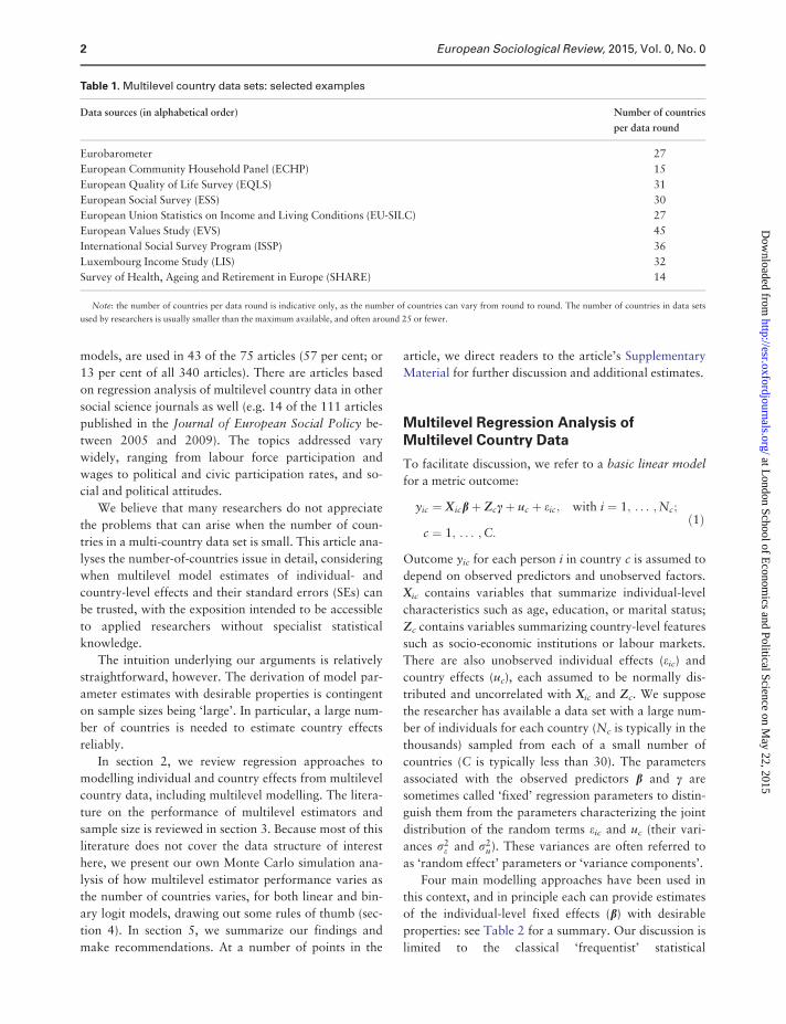
Some of the multi-country data sets that are com-

monly used in contemporary social science research are

listed in Table 1. In each of them, there is a natural hier-

archy with observations at the individual level nested

within a higher level (countries). The data sets typically

contain thousands of individuals per country but the

number of countries is small, at most around 30. The

number of countries used in analysis is often fewer,

nearer 20 and sometimes less, because of missing data or

analytical focus.

Multi-country data sets are attractive because they

offer a means of quantifying the extent to which differ-

ences in outcomes reflect differences in the effects of

country-specific features of demographic structure, la-

bour markets, and other socio-economic institutions

such as tax-benefit systems, which are distinct from the

differences in outcomes associated with variations in the

characteristics of the individuals themselves. That is,

multi-country data sets potentially provide information

about ‘country effects’ as well as ‘individual effects’, and

also about interactions between them (‘cross-level

effects’).

The popularity of regression analysis of multilevel

country data is illustrated by the European Sociological

Review. Of the 340 articles published between 2005 and

2012, approximately 75 exploit multilevel data sets with

individual respondents within countries. Multilevel

models, also known as hierarchical models or mixed

VC The Author 2015. Published by Oxford University Press.

This is an Open Access article distributed under the terms of the Creative Commons Attribution License (http://creativecommons.org/licenses/by/4.0/),

which permits unrestricted reuse, distribution, and reproduction in any medium, provided the original work is properly cited.

European Sociological Review, 2015, 1–20

doi: 10.1093/esr/jcv059

Original Article

European Sociological Review Advance Access published May 8, 2015

at London School of E

conomics and Political Science on M

ay 22, 2015http://esr.oxfordjournals.org/

Dow

nloaded from

http://www.oxfordjournals.org/

http://esr.oxfordjournals.org/

models, are used in 43 of the 75 articles (57 per cent; or

13 per cent of all 340 articles). There are articles based

on regression analysis of multilevel country data in other

social science journals as well (e.g. 14 of the 111 articles

published in the Journal of European Social Policy be-

tween 2005 and 2009). The topics addressed vary

widely, ranging from labour force participation and

wages to political and civic participation rates, and so-

cial and political attitudes.

We believe that many researchers do not appreciate

the problems that can arise when the number of coun-

tries in a multi-country data set is small. This article ana-

lyses the number-of-countries issue in detail, considering

when multilevel model estimates of individual- and

country-level effects and their standard errors (SEs) can

be trusted, with the exposition intended to be accessible

to applied researchers without specialist statistical

knowledge.

The intuition underlying our arguments is relatively

straightforward, however. The derivation of model par-

ameter estimates with desirable properties is contingent

on sample sizes being ‘large’. In particular, a large num-

ber of countries is needed to estimate country effects

reliably.

In section 2, we review regression approaches to

modelling individual and country effects from multilevel

country data, including multilevel modelling. The litera-

ture on the performance of multilevel estimators and

sample size is reviewed in section 3. Because most of this

literature does not cover the data structure of interest

here, we present our own Monte Carlo simulation ana-

lysis of how multilevel estimator performance varies as

the number of countries varies, for both linear and bin-

ary logit models, drawing out some rules of thumb (sec-

tion 4). In section 5, we summarize our findings and

make recommendations. At a number of points in the

article, we direct readers to the article’s Supplementary

Material for further discussion and additional estimates.

Multilevel Regression Analysis ofMultilevel Country Data

To facilitate discussion, we refer to a basic linear model

for a metric outcome:

yic ¼ X icbþ Zccþ uc þ eic; with i ¼ 1; . . . ;Nc;

c ¼ 1; . . . ;C:ð1Þ

Outcome yic for each person i in country c is assumed to

depend on observed predictors and unobserved factors.

Xic contains variables that summarize individual-level

characteristics such as age, education, or marital status;

Zc contains variables summarizing country-level features

such as socio-economic institutions or labour markets.

There are also unobserved individual effects (eic) and

country effects (uc), each assumed to be normally dis-

tributed and uncorrelated with Xic and Zc. We suppose

the researcher has available a data set with a large num-

ber of individuals for each country (Nc is typically in the

thousands) sampled from each of a small number of

countries (C is typically less than 30). The parameters

associated with the observed predictors b and c are

sometimes called ‘fixed’ regression parameters to distin-

guish them from the parameters characterizing the joint

distribution of the random terms eic and uc (their vari-

ances r2e and r2

u). These variances are often referred to

as ‘random effect’ parameters or ‘variance components’.

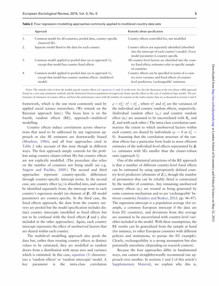
Four main modelling approaches have been used in

this context, and in principle each can provide estimates

of the individual-level fixed effects (b) with desirable

properties: see Table 2 for a summary. Our discussion is

limited to the classical ‘frequentist’ statistical

Table 1. Multilevel country data sets: selected examples

Data sources (in alphabetical order) Number of countries

per data round

Eurobarometer 27

European Community Household Panel (ECHP) 15

European Quality of Life Survey (EQLS) 31

European Social Survey (ESS) 30

European Union Statistics on Income and Living Conditions (EU-SILC) 27

European Values Study (EVS) 45

International Social Survey Program (ISSP) 36

Luxembourg Income Study (LIS) 32

Survey of Health, Ageing and Retirement in Europe (SHARE) 14

Note: the number of countries per data round is indicative only, as the number of countries can vary from round to round. The number of countries in data sets

used by researchers is usually smaller than the maximum available, and often around 25 or fewer.

2 European Sociological Review, 2015, Vol. 0, No. 0




Dow

nloaded from

http://esr.oxfordjournals.org/lookup/suppl/doi:10.1093/esr/jcv059/-/DC1



framework, which is the one most commonly used by

applied social science researchers. (We remark on the

Bayesian approach later.) The focus here is on the

fourth, random effects (RE), approach—multilevel

modelling.

Country effects induce correlations across observa-

tions that need to be addressed by any regression ap-

proach or else SE estimates are downwardly biased

(Moulton, 1986), and all four approaches cited in

Table 2 take account of this issue though in different

ways. The first approach simply controls for the prob-

lem using country-cluster-robust SEs but country effects

are not explicitly modelled. (The procedure also relies

on the number of countries not being small: see e.g.

Angrist and Pischke, 2009.) The second and third

approaches represent country-specific differences

through country-specific intercept terms. In the second

case, any country effect (uc) is absorbed into, and cannot

be identified separately from, the intercept term in each

country’s regression model (an element of b). All model

parameters are country-specific. In the third case, the

fixed effects approach, the data from the country sur-

veys are pooled but the model specification includes dis-

tinct country intercepts (modelled as fixed effects but

not to be confused with the fixed effects b and c also

included in the other approaches). Again, each country

intercept represents the effect of unobserved factors that

are shared within each country.

The multilevel modelling approach also pools the

data but, rather than treating country effects as distinct

values to be estimated, they are modelled as random

draws from a distribution with mean zero and variance

which is estimated. In this case, equation (1) character-

izes a ‘random effects’ or ‘random intercepts’ model. A

key parameter is the intra-class correlation

q ¼ r2u= r2

e þ r2u

� �, where r2

e and r2u are the variances of

the individual and country random effects, respectively.

(Individual random effect (eic) and country random

effect (uc) are assumed to be uncorrelated with Xic and

Zc and with each other.) The intra-class correlation sum-

marizes the extent to which unobserved factors within

each country are shared by individuals (q ! 0 as r2u !

0). Assuming that the correlation structure of the ran-

dom effects has a particular form leads to more efficient

estimates of the individual-level effects represented by b,

i.e. estimates with SEs smaller than the cluster-robust

ones (approach 1).

One of the substantial attractions of the RE approach

is that a number of different country-level fixed effects

can be estimated by using appropriately defined coun-

try-level predictors (elements of Zc), though the number

of parameters that can be reliably fitted is constrained

by the number of countries. Any remaining unobserved

country effects (uc) are treated as being generated by

some common mechanism and so are ‘exchangeable’ be-

tween countries (Snijders and Bosker, 2012: pp. 46–47).

The regression intercept is a population average (for ex-

ample, a common European intercept if the data are

from EU countries), and deviations from this average

are assumed to be uncorrelated with country-level vari-

ables included in the model. With these assumptions, the

RE results can be generalized from the sample at hand

(for instance, to other European countries with different

policies and institutions, to pursue the EU example).

Clearly, exchangeability is a strong assumption but also

potentially unrealistic (depending on research context).

Because the four approaches differ in fundamental

ways, one cannot straightforwardly recommend one ap-

proach over another. In sections 1 and 2 of this article’s

Supplementary Material, we explain why this is,

Table 2. Four regression modelling approaches commonly applied to multilevel country data sets

Approach Remarks about specification

1. Common model for all countries, pooled data, country-specific

clustered SEs

Country effects controlled for, not modelled

2. Separate model fitted to the data for each country Country effects not separately identified (absorbed

into the intercept of each country’s model). Every

model parameter is country-specific

3. Common model applied to pooled data (as in approach 1),

except that model has country fixed effects

All country-level factors are absorbed into the coun-

try fixed effect; estimates refer to specific sample

of countries

4. Common model applied to pooled data (as in approach 1),

except that model has country random effects (multilevel

model)

Country effects can be specified in terms of a coun-

try error variance and fixed effects of country-

level predictors; ‘exchangeable’ estimates

Notes: The remarks refer to how the models specify country effects (cf. equations (1) and (2) in the text). See also the discussion in the text about a fifth approach

(based on a two-step estimation method) and the distinction between population-averaged and cluster-specific effects in the case of multilevel logit models. The per-

formance of estimators of country effects, and how this performance varies with the number of countries in the multi-country data set, is discussed in sections 3 and 4.

European Sociological Review, 2015, Vol. 0, No. 0 3




Dow

nloaded from



referring to modelling goals and statistical performance

of the various estimators, and also discuss the

approaches at greater length. We conclude that analysts

primarily interested in the individual-level fixed effects

associated with observed predictors (b) may favour one

of the first three approaches. However, multilevel mod-

elling is the natural choice if the interest is in the effects

(c) of country-level predictors or the variance compo-

nent structure. Non-economist social scientists have

tended to favour the multilevel modelling approach, as-

sessing country ‘effects’ in terms of either country fixed

effects or in terms of the proportion of the outcome vari-

ance explained by the country variance component(s).

See for example Snijder and Bosker (2012: chapter 4).

Multilevel modelling approaches are the focus in the rest

of the article.

It is also instructive to consider a fifth approach in

which estimation is undertaken in two steps (see section

3 of the Supplementary Material for further discussion).

In the first step of the two-step approach, one fits equa-

tion (1) using ordinary least squares and country-specific

fixed effects (as in approach 3). Country-level effects (c)

are ascertained from the second step in which the fitted

country intercepts from step 1 are regressed on the coun-

try-level predictors (Zc). This two-step procedure has

several advantages. First, it highlights the sources of vari-

ation in the data and shows why a small number of coun-

tries can affect the reliability of estimates (the sample size

in the second step is the number of countries). Second,

the estimates are unbiased (with correct SEs) and so can

be used to benchmark the other methods. Third, the

two-step method leads naturally to a graphical summary

of country-level variations in outcomes in which one

plots the country intercepts fitted at step 1 against elem-

ents of Zc (Bowers and Drake, 2005; Kedar and Shively,

2005). We return to this third property in section 5.

Two-step estimation of hierarchical structures dates

back to at least Hanushek (1974) and Saxonhouse (1976)

among economists, but the method has been periodically

rediscovered. Borjas and Sueyoshi (1994) presented a

two-step estimator for the probit model, and other pro-

ponents include Card (1995), Jusko and Shively (2005),

and other papers in a special issue of Political Analysis

(Kedar and Shively 2005). Donald and Lang (2007) dis-

cuss the statistical properties of the two-step estimator

(compared with Generalized Least Squares (GLS)) in de-

tail. For textbook discussion, see Wooldridge (2010:

chapter 20). The two-step estimator is effectively what is

done in meta-analysis in which estimates and SEs from a

number of studies are combined to derive an overall effect

estimate. For more on these parallels, see Hox (2010:

chapter 11).

The various approaches just set out, and our discus-

sion of them, also apply to non-linear models. The basic

logit model for a binary outcome that is analogous to

equation (1) for metric outcomes is of the following form:

log pic= 1–picð Þ½ � ¼ X icbþ Zccþ uc þ eic;

with i ¼ 1; . . . ;Nc; c ¼ 1; . . . ;C;(2)

where pic is the probability of the binary outcome for

person i in country c and variance r2u is normalized to

equal p2/3. However, there is an important conceptual

difference between the logistic and linear multilevel

models that is distinct from issues of estimator perform-

ance. This concerns the nature of the effects that the re-

searcher is interested in. Given estimates of multilevel

logistic model parameters, researchers may be interested

in population-averaged (‘marginal’) effects or cluster-

specific (‘conditional’) effects. In the former case, the

interest is in the impact on the outcome probability of a

change in an individual- or country-level characteristic

which is the average across the distribution of unob-

served characteristics (hence the population average

label). In latter case, the interest is in the impact on out-

come probabilities of a change in an individual- or

country-level characteristic for an individual with a

specific set of characteristics, observed and unobserved.

(In the analogous linear model, the two types of effect

coincide.) For more about the distinction between popu-

lation-averaged and cluster-specific effects, see for

example Molenberghs and Verbeke (2005) or Neuhaus,

Kalbfleisch and Hauck (1991). In our examination of

multilevel logit models, we consider estimation of

cluster-specific effects (represented by b and c in

equation (2)) as these have been the focus of interest of

virtually all the applied social science research in the

literature that we cited in the Introduction.

Our Monte Carlo simulation analysis assesses the

performance of estimators not only for basic linear and

logit models, but also ‘extended’ linear and logit models

in which the specifications set out in equations (1) and

(2) are supplemented to allow for individual variation in

two individual-level fixed effects (‘random slopes’) and

also the effect of an individual-level predictor varies with

the size of a country-level fixed effect (a cross-level inter-

action). We focus on the results for the basic models here

(section 4); detailed results for the extended models are

presented in section 7 of the Supplementary Material.

How Many Countries Are Required forReliable Estimates? Literature Review

In this section, we review theoretical results and Monte

Carlo simulation evidence to summarize what is known





Dow

nloaded from




about the statistical properties of standard multilevel

model estimators. Unless stated otherwise, the estima-

tors we refer to are Restricted (or Residual) Maximum

Likelihood (REML) for mixed linear models and

Maximum Likelihood (ML) for mixed logit models.

These are the most commonly used estimators nowadays

and also have the best properties (among classical statis-

tical estimators): see the review by Hox (2010: chapters

3 and 6), for example. We refer to some other estimators

later.

In general, the statistical properties of these estima-

tors are well-defined only when both the number of

groups (countries here) and group sizes (numbers of in-

dividuals) are large, in which case estimates of param-

eters and their sampling variability are consistent (they

converge to their true values with sufficiently large sam-

ples) and are asymptotically normally distributed. That

is, with samples that are large in both the individuals

and countries dimensions, estimators are accurate and

there can be reliable inference about parameter values

(employing the estimates of the parameters and of their

SEs). This is the case for both linear and logit mixed

models.

What if the number of groups is small? For the linear

mixed model, estimates of the fixed effects (b and c in

equation (1)) are unbiased (Kackar and Harville, 1981,

1984). However, if the number of groups is small, and

even if the group sizes are large, estimates of the vari-

ance components and of their SEs are imprecise and

likely to be biased downwards (Raudenbush and Bryk,

2002: p. 283; Hox, 2010: p. 233). Estimates of the SEs

of fixed parameters are also affected by the uncertainty

in the variance estimates: they are biased downwards

and the distribution of test statistics is unknown

(Raudenbush and Bryk, 2002: p. 282). There are some

methods available to derive better estimates of the SEs

of the fixed effects and hence undertake more reliable in-

ference about them (see below). However, these meth-

ods provide little comfort to most applied social

scientists because these researchers are also particularly

interested in the magnitudes of, and inference about,

country-level variance components.

The conclusions about estimator performance cited

in the previous paragraph also apply to logit mixed

models, but with additional stings in the tail. That is,

there are no theoretical results available concerning the

bias of fixed effect estimators; fixed effect SEs are biased

downwards (but there are no convenient bias-correction

methods); and variance component estimators and their

SEs are biased downwards, often substantially.

The upshot is that, if the number of countries is

small, estimates of ‘country effects’ produced may be

unreliable. Although estimates of the effect of a country-

level predictor may be unbiased, assessments of the stat-

istical significance of the effect and inference more

generally will be unreliable (SEs are too small and confi-

dence intervals (CIs) too narrow). Country variance

components will be under-estimated, providing incorrect

estimates of intraclass correlations (ICCs), and inference

about them is also unreliable.

Specific and consistent guidance to modellers about

the number of groups required to avoid the problems

cited is difficult to find. The Centre for Multilevel

Modelling’s FAQ on sample sizes for multilevel modelling

states that ‘[r]ules of thumb such as only doing multilevel

modelling with 15 or 30 or 50 level 2 units can be found

and are often personal opinions based on personal experi-

ence and varying reasons’ (Centre for Multilevel

Modelling, 2011). Most multilevel modelling textbooks

mention the issues and also sometimes cite rules of

thumb, recommending anywhere between 10 and 50

groups as a minimum. They stress that the minimum

number depends on application-specific factors like the

number of group-level predictors (Raudenbush and Bryk,

2002: p. 267) and whether interest is focussed on the co-

efficients on the fixed regression predictors or the param-

eters describing random effects such as variance

components (Hox, 2010: p. 235). Moreover, advice

about sample size is often bound up with considerations

of the cost of primary data collection and survey design

ex ante: see Snijders and Bosker (2012: chapter 11).

However, these cost issues are not relevant for secondary

analysis of the many multilevel country data sets that are

already in existence.

Most discussion of the small group size issue is based

on Monte Carlo analysis of simulated data because the-

ory does not provide specific guidance. See for instance

the review by Hox (2010: chapter 12), who also summa-

rizes a number of earlier unpublished studies. A number

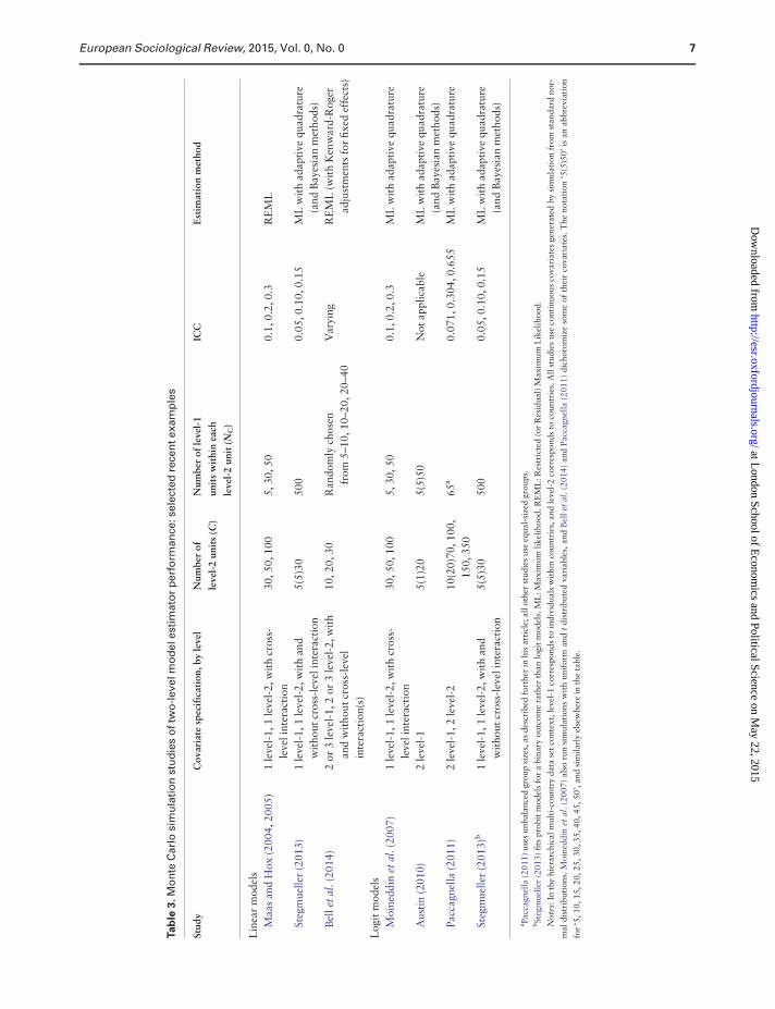
of recent Monte Carlo studies of two-level linear and

logit models are listed in Table 3, together with a sum-

mary of their principal design features.

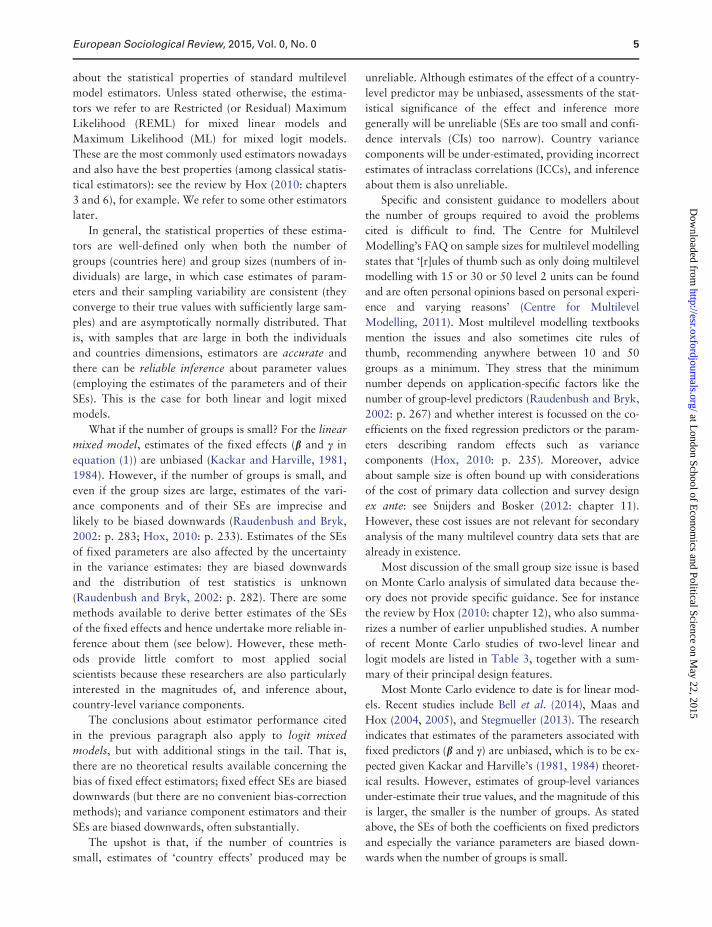
Most Monte Carlo evidence to date is for linear mod-

els. Recent studies include Bell et al. (2014), Maas and

Hox (2004, 2005), and Stegmueller (2013). The research

indicates that estimates of the parameters associated with

fixed predictors (b and c) are unbiased, which is to be ex-

pected given Kackar and Harville’s (1981, 1984) theoret-

ical results. However, estimates of group-level variances

under-estimate their true values, and the magnitude of this

is larger, the smaller is the number of groups. As stated

above, the SEs of both the coefficients on fixed predictors

and especially the variance parameters are biased down-

wards when the number of groups is small.





Dow

nloaded from


Based on their simulation evidence, Maas and Hox’s

(2004) rules of thumb for multilevel linear models are:

10 groups are sufficient for unbiased estimates of the b

and c, at least 30 groups are needed for good variance

estimates, and at least 50 groups are required for accur-

ate SE estimates especially for those associated with

(co)variance component parameters.

There is less evidence for multilevel logit models than

for linear models but the few existing studies suggest

broadly similar conclusions: see, for example, Austin

(2010), Moineddin, Matheson and Glazier (2007),

Paccagnella (2011), and Stegmueller (2013). With a

small number of groups, estimates of the fixed effect

parameters in binary logit or probit models are generally

unbiased—though not always for level-2 fixed effects

(Moineddin, Matheson and Glazier, 2007; Paccagnella

2011). Estimates of variance components are biased

downwards with the magnitude of the problem depend-

ing on the type of estimator used to maximize the likeli-

hood (adaptive quadrature appears to provide the least

bad estimates), and the SEs associated with both fixed

and variance parameters are too small. Stegmueller

(2013) urges caution in using classical ML methods with

<10 or 15 groups, especially when the model includes

cross-level interactions and random coefficients,

whereas Moineddin, Matheson and Glazier (2007) rec-

ommend using at least 50 groups.

One caveat regarding all of the Monte Carlo studies

is that their conclusions are potentially sensitive to

model specification, including choices of parameter val-

ues and numbers and types of predictors. Also, studies

have typically been based on models with relatively sim-

ple specifications: see Table 3. The result is that the sam-

ple sizes and data distributions used in these studies are

rarely similar to what is used in the hierarchical cross-

national data context. For example, Maas and Hox

(2004) specify a linear model for a continuous outcome

with a random intercept, a single individual-level regres-

sor (with random slope), a single group-level regressor,

and an interaction of the two (both regressors are nor-

mally distributed). Austin (2010) specifies a logit model

but with an even simpler specification, consisting of a

random intercept and two (joint normally distributed)

individual-level regressors. Few studies investigate esti-

mator performance using data with combinations of

group sizes and numbers of groups that correspond to

those typical in the hierarchical cross-national data con-

text. Stegmueller (2013) is the exception, but his model

specifications and data generation process are relatively

simple, and his analysis focuses almost entirely on fixed

effects parameters with no discussion of variance param-

eters (which are also of interest to applied social science

researchers). In addition, Stegmueller uses ML estima-

tors for all models including his linear models, for which

the recommended estimator is REML (see above).

In our own Monte Carlo analysis in the next section,

we use study designs with sample sizes, simulated data

distributions, and model specifications that are more

like those in real-life multilevel country data. This is par-

ticularly important because the number of countries in

the multilevel country data sets typically available

(Table 1) falls within the range identified by these

Monte Carlo studies as providing unreliable estimates.

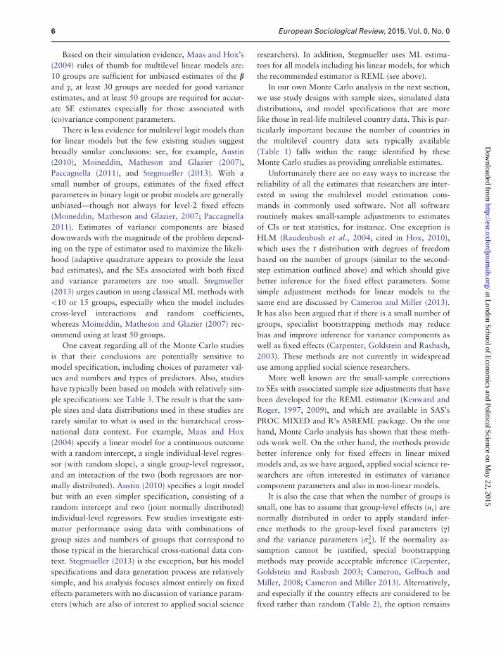
Unfortunately there are no easy ways to increase the

reliability of all the estimates that researchers are inter-

ested in using the multilevel model estimation com-

mands in commonly used software. Not all software

routinely makes small-sample adjustments to estimates

of CIs or test statistics, for instance. One exception is

HLM (Raudenbush et al., 2004, cited in Hox, 2010),

which uses the t distribution with degrees of freedom

based on the number of groups (similar to the second-

step estimation outlined above) and which should give

better inference for the fixed effect parameters. Some

simple adjustment methods for linear models to the

same end are discussed by Cameron and Miller (2013).

It has also been argued that if there is a small number of

groups, specialist bootstrapping methods may reduce

bias and improve inference for variance components as

well as fixed effects (Carpenter, Goldstein and Rasbash,

2003). These methods are not currently in widespread

use among applied social science researchers.

More well known are the small-sample corrections

to SEs with associated sample size adjustments that have

been developed for the REML estimator (Kenward and

Roger, 1997, 2009), and which are available in SAS’s

PROC MIXED and R’s ASREML package. On the one

hand, Monte Carlo analysis has shown that these meth-

ods work well. On the other hand, the methods provide

better inference only for fixed effects in linear mixed

models and, as we have argued, applied social science re-

searchers are often interested in estimates of variance

component parameters and also in non-linear models.

It is also the case that when the number of groups is

small, one has to assume that group-level effects (uc) are

normally distributed in order to apply standard infer-

ence methods to the group-level fixed parameters (c)

and the variance parameters (r2u). If the normality as-

sumption cannot be justified, special bootstrapping

methods may provide acceptable inference (Carpenter,

Goldstein and Rasbash 2003; Cameron, Gelbach and

Miller, 2008; Cameron and Miller 2013). Alternatively,

and especially if the country effects are considered to be

fixed rather than random (Table 2), the option remains





Dow

nloaded from


Tab

le3.M

on

teC

arl

osi

mu

lati

on

stu

die

so

ftw

o-l

ev

elm

od

ele

stim

ato

rp

erf

orm

an

ce:se

lect

ed

rece

nt

ex

am

ple

s

Stu

dy

Covari

ate

spec

ific

ati

on,by

level

Num

ber

of

level

-2unit

s(C

)

Num

ber

of

level

-1

unit

sw

ithin

each

level

-2unit

(NC)

ICC

Est

imati

on

met

hod

Lin

ear

model

s

Maas

and

Hox

(2004,2005)

1le

vel

-1,1

level

-2,w

ith

cross

-

level

inte

ract

ion

30,50,100

5,30,50

0.1

,0.2

,0.3

RE

ML

Ste

gm

uel

ler

(2013)

1le

vel

-1,1

level

-2,w

ith

and

wit

hout

cross

-lev

elin

tera

ctio

n

5(5

)30

500

0.0

5,0.1

0,0.1

5M

Lw

ith

adapti

ve

quadra

ture

(and

Bayes

ian

met

hods)

Bel

let

al.(2

014)

2or

3le

vel

-1,2

or

3le

vel

-2,w

ith

and

wit

hout

cross

-lev

el

inte

ract

ion(s

)

10,20,30

Random

lych

ose

n

from

5–10,10–20,20–40

Vary

ing

RE

ML

(wit

hK

enw

ard

-Roger

adju

stm

ents

for

fixed

effe

cts)

Logit

model

s

Moin

eddin

etal

.(2

007)

1le

vel

-1,1

level

-2,w

ith

cross

-

level

inte

ract

ion

30,50,100

5,30,50

0.1

,0.2

,0.3

ML

wit

hadapti

ve

quadra

ture

Aust

in(2

010)

2le

vel

-15(1

)20

5(5

)50

Not

applica

ble

ML

wit

hadapti

ve

quadra

ture

(and

Bayes

ian

met

hods)

Pacc

agnel

la(2

011)

2le

vel

-1,2

level

-210(2

0)7

0,100,

150,350

65

a0.0

71,0.3

04,0.6

55

ML

wit

hadapti

ve

quadra

ture

Ste

gm

uel

ler

(2013)b

1le

vel

-1,1

level

-2,w

ith

and

wit

hout

cross

-lev

elin

tera

ctio

n

5(5

)30

500

0.0

5,0.1

0,0.1

5M

Lw

ith

adapti

ve

quadra

ture

(and

Bayes

ian

met

hods)

aPacc

agnel

la(2

011)

use

sunbala

nce

dgro

up

size

s,as

des

crib

edfu

rther

inhis

art

icle

;all

oth

erst

udie

suse

equal-

size

dgro

ups.

bSte

gm

uel

ler

(2013)

fits

pro

bit

model

sfo

ra

bin

ary

outc

om

era

ther

than

logit

model

s.M

L:M

axim

um

likel

ihood.R

EM

L:R

estr

icte

d(o

rR

esid

ual)

Maxim

um

Lik

elih

ood.

Note

s:In

the

hie

rarc

hic

alm

ult

i-co

untr

ydata

set

conte

xt,

level

-1co

rres

ponds

toin

div

iduals

wit

hin

countr

ies,

and

level

-2co

rres

ponds

toco

untr

ies.

All

studie

suse

conti

nuous

covari

ate

sgen

erate

dby

sim

ula

tion

from

standard

nor-

mal

dis

trib

uti

ons.

Moin

eddin

etal

.(2

007)

als

oru

nsi

mula

tions

wit

hunif

orm

and

tdis

trib

ute

dvari

able

s,and

Bel

let

al.

(2014)

and

Pacc

agnel

la(2

011)

dic

hoto

miz

eso

me

of

thei

rco

vari

ate

s.T

he

nota

tion

‘5(5

)50’

isan

abbre

via

tion

for

‘5,10,15,20,25,30,35,40,45,50’,

and

sim

ilarl

yel

sew

her

ein

the

table

.





Dow

nloaded from


to use graphical methods to describe estimates of cross-

country differences from step 1 of a two-stage approach

(Bowers and Drake 2005).

How Many Countries are Needed forReliable Estimates? Monte CarloSimulation Analysis

We use Monte Carlo simulations to assess how large the

number of countries needs to be to derive accurate esti-

mates of model parameters and their SEs from the stand-

ard multilevel model estimators. For several reasons,

previous analysis does not necessarily translate to typical

multi-country data set applications. First, previous stud-

ies have mainly been concerned with education and

health research contexts that involve moderate numbers

of both groups and numbers of observations within

groups. Thus they do not usually consider the sample

sizes of most relevance to cross-country researchers, i.e.

a number of groups often well below 30 and group sizes

of many hundreds (at least). Second, previous studies

use simple, rather unrealistic, model specifications, typ-

ically including only two or three ‘well-behaved’ (nor-

mally distributed) regressors. In contrast, we consider

both linear and non-linear models using data structures

that are similar to those found in multi-country data

sets, we employ a greater range in the number of coun-

tries, and we also give greater attention to various as-

pects of accuracy than previous research—this turns out

to be relevant when assessing the properties of estimates

of some individual-level and country-level effects (see

below). We include binary, categorical, and continuous

variables in our simulated data sets, and do not impose

normality.

Our simulation results are based on two-level linear

and logit models. In this article, we focus on a ‘basic’

specification with random intercepts corresponding to

equation (1). The regressors include a constant (inter-

cept), individual-level fixed effects, a country-level fixed

effect, and a random country intercept. (The model also

includes an individual-specific error term.) In common

with most social science applications, we assume that

the random effects are uncorrelated with each other. To

make the models more concrete, we refer to the outcome

variables for the linear and non-linear models as ‘hours’

(of work) and (labour force) ‘participation’, respectively.

We shall also refer briefly to our Monte Carlo analysis

of ‘extended’ linear and logit models that include the

same regressors but add two cross-level interactions,

and two random slopes. Further details of the results for

these models and Stata code for running all of the

simulations are provided in the Supplementary Material

(sections 7 and 9).

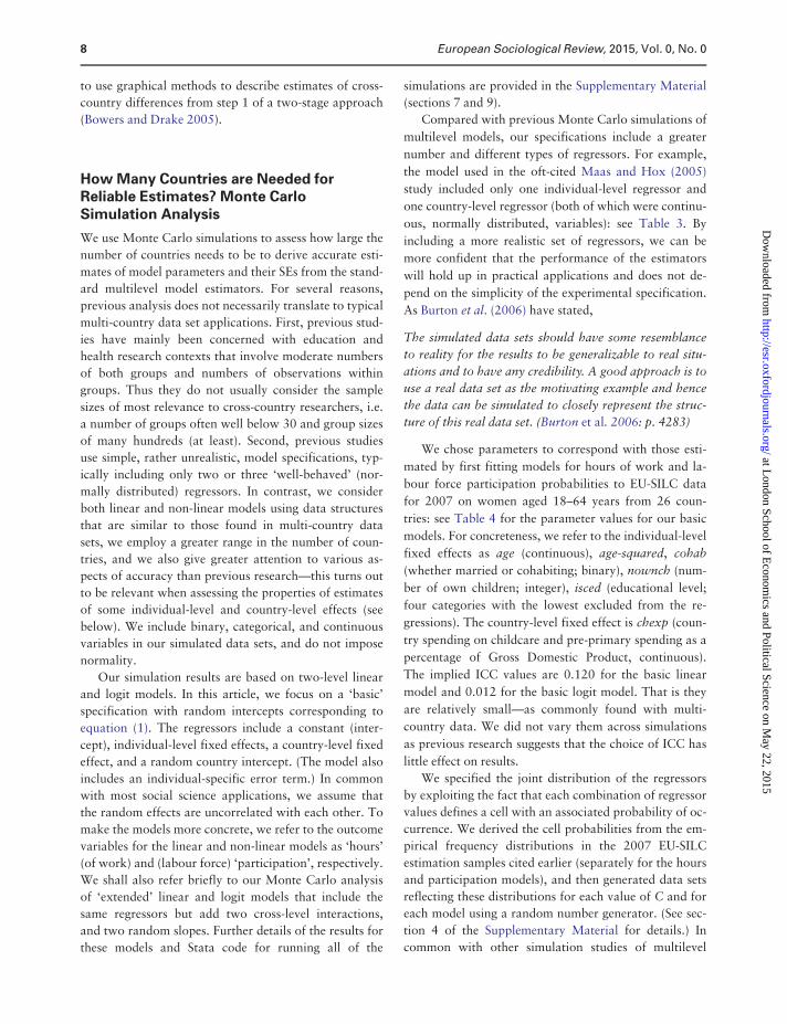
Compared with previous Monte Carlo simulations of

multilevel models, our specifications include a greater

number and different types of regressors. For example,

the model used in the oft-cited Maas and Hox (2005)

study included only one individual-level regressor and

one country-level regressor (both of which were continu-

ous, normally distributed, variables): see Table 3. By

including a more realistic set of regressors, we can be

more confident that the performance of the estimators

will hold up in practical applications and does not de-

pend on the simplicity of the experimental specification.

As Burton et al. (2006) have stated,

The simulated data sets should have some resemblance

to reality for the results to be generalizable to real situ-

ations and to have any credibility. A good approach is to

use a real data set as the motivating example and hence

the data can be simulated to closely represent the struc-

ture of this real data set. (Burton et al. 2006: p. 4283)

We chose parameters to correspond with those esti-

mated by first fitting models for hours of work and la-

bour force participation probabilities to EU-SILC data

for 2007 on women aged 18–64 years from 26 coun-

tries: see Table 4 for the parameter values for our basic

models. For concreteness, we refer to the individual-level

fixed effects as age (continuous), age-squared, cohab

(whether married or cohabiting; binary), nownch (num-

ber of own children; integer), isced (educational level;

four categories with the lowest excluded from the re-

gressions). The country-level fixed effect is chexp (coun-

try spending on childcare and pre-primary spending as a

percentage of Gross Domestic Product, continuous).

The implied ICC values are 0.120 for the basic linear

model and 0.012 for the basic logit model. That is they

are relatively small—as commonly found with multi-

country data. We did not vary them across simulations

as previous research suggests that the choice of ICC has

little effect on results.

We specified the joint distribution of the regressors

by exploiting the fact that each combination of regressor

values defines a cell with an associated probability of oc-

currence. We derived the cell probabilities from the em-

pirical frequency distributions in the 2007 EU-SILC

estimation samples cited earlier (separately for the hours

and participation models), and then generated data sets

reflecting these distributions for each value of C and for

each model using a random number generator. (See sec-

tion 4 of the Supplementary Material for details.) In

common with other simulation studies of multilevel





Dow

nloaded from




models, the joint distribution of the regressors is the

same across replications for each value of C. The mean

values of the regressors and outcome variables from the

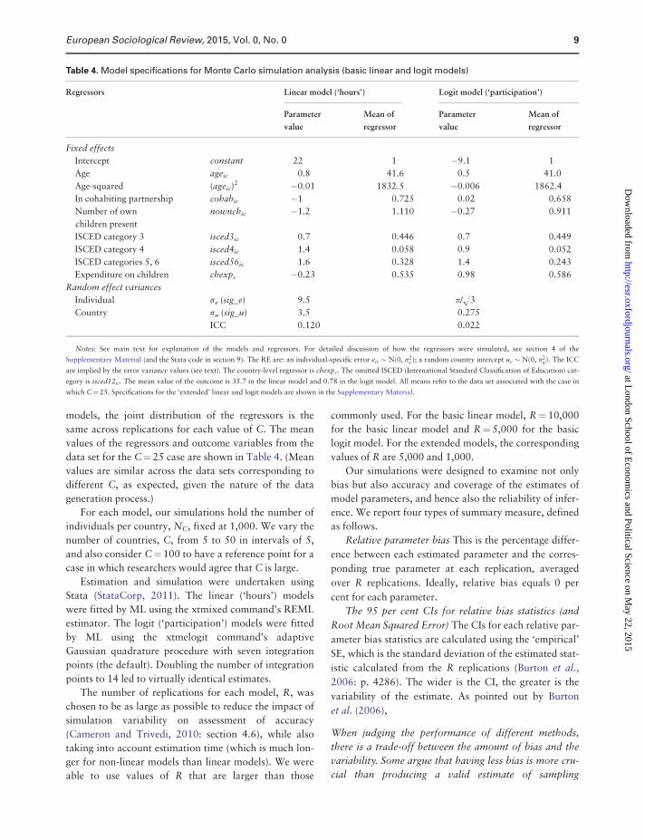
data set for the C¼ 25 case are shown in Table 4. (Mean

values are similar across the data sets corresponding to

different C, as expected, given the nature of the data

generation process.)

For each model, our simulations hold the number of

individuals per country, NC, fixed at 1,000. We vary the

number of countries, C, from 5 to 50 in intervals of 5,

and also consider C¼100 to have a reference point for a

case in which researchers would agree that C is large.

Estimation and simulation were undertaken using

Stata (StataCorp, 2011). The linear (‘hours’) models

were fitted by ML using the xtmixed command’s REML

estimator. The logit (‘participation’) models were fitted

by ML using the xtmelogit command’s adaptive

Gaussian quadrature procedure with seven integration

points (the default). Doubling the number of integration

points to 14 led to virtually identical estimates.

The number of replications for each model, R, was

chosen to be as large as possible to reduce the impact of

simulation variability on assessment of accuracy

(Cameron and Trivedi, 2010: section 4.6), while also

taking into account estimation time (which is much lon-

ger for non-linear models than linear models). We were

able to use values of R that are larger than those

commonly used. For the basic linear model, R¼ 10,000

for the basic linear model and R¼5,000 for the basic

logit model. For the extended models, the corresponding

values of R are 5,000 and 1,000.

Our simulations were designed to examine not only

bias but also accuracy and coverage of the estimates of

model parameters, and hence also the reliability of infer-

ence. We report four types of summary measure, defined

as follows.

Relative parameter bias This is the percentage differ-

ence between each estimated parameter and the corres-

ponding true parameter at each replication, averaged

over R replications. Ideally, relative bias equals 0 per

cent for each parameter.

The 95 per cent CIs for relative bias statistics (and

Root Mean Squared Error) The CIs for each relative par-

ameter bias statistics are calculated using the ‘empirical’

SE, which is the standard deviation of the estimated stat-

istic calculated from the R replications (Burton et al.,

2006: p. 4286). The wider is the CI, the greater is the

variability of the estimate. As pointed out by Burton

et al. (2006),

When judging the performance of different methods,

there is a trade-off between the amount of bias and the

variability. Some argue that having less bias is more cru-

cial than producing a valid estimate of sampling

Table 4. Model specifications for Monte Carlo simulation analysis (basic linear and logit models)

Regressors Linear model (‘hours’) Logit model (‘participation’)

Parameter

value

Mean of

regressor

Parameter

value

Mean of

regressor

Fixed effects

Intercept constant 22 1 �9.1 1

Age ageic 0.8 41.6 0.5 41.0

Age-squared (ageic)2 �0.01 1832.5 �0.006 1862.4

In cohabiting partnership cohabic �1 0.725 0.02 0.658

Number of own

children present

nownchic �1.2 1.110 �0.27 0.911

ISCED category 3 isced3ic 0.7 0.446 0.7 0.449

ISCED category 4 isced4ic 1.4 0.058 0.9 0.052

ISCED categories 5, 6 isced56ic 1.6 0.328 1.4 0.243

Expenditure on children chexpc �0.23 0.535 0.98 0.586

Random effect variances

Individual re (sig_e) 9.5 p/H3

Country ru (sig_u) 3.5 0.275

ICC 0.120 0.022

Notes: See main text for explanation of the models and regressors. For detailed discussion of how the regressors were simulated, see section 4 of the

Supplementary Material (and the Stata code in section 9). The RE are: an individual-specific error eic � N(0, r2e ); a random country intercept uc � N(0, r2

u). The ICC

are implied by the error variance values (see text). The country-level regressor is chexpc. The omitted ISCED (International Standard Classification of Education) cat-

egory is isced12ic. The mean value of the outcome is 35.7 in the linear model and 0.78 in the logit model. All means refer to the data set associated with the case in

which C¼25. Specifications for the ‘extended’ linear and logit models are shown in the Supplementary Material.





Dow

nloaded from




variance . . . However, methods that result in an un-

biased estimate with large variability or conversely a

biased estimate with little variability may be considered

of little practical use. (Burton et al., 2006: p. 4286.)

We demonstrate below that the combination of lack of

bias but large variability is a feature of country-level

fixed effects estimates from multi-country data sets.

Researchers sometimes use composite measures of esti-

mator accuracy that combine summaries of bias and

variability, the most common of which is the Root

Mean Squared Error (RMSE) statistic associated with

each parameter (the square root of the sum of absolute

bias squared and the empirical SE squared). We have

also calculated RMSE statistics for our basic model

simulations, and they yield conclusions about accuracy

consistent with the discussion below (see section 6 of the

Supplementary Material).

Relative SE bias We compare the empirical SE

described above with the ‘analytical’ SE reported by the

software and averaged over R replications (Greene,

2004). Relative SE bias is the percentage difference be-

tween the analytical and empirical SEs, assuming the

empirical SE is an accurate estimate of the true SE.

Ideally, the relative bias equals 0 per cent for each SE.

Non-coverage rate To assess inference performance

overall, we calculate a 95 per cent CI for each estimated

parameter assuming normality (Maas and Hox, 2005: p.

89). A non-coverage indicator variable was set equal to

zero if this CI included the true parameter and one if it

did not. The average over R replications of this variable

is the non-coverage rate. Ideally, the non-coverage rate

for a 95 per cent CI is 0.05. Rates greater than 0.05 indi-

cate that the software-estimated CI is too narrow and

significance tests on parameters will be anticonservative.

Most simulation studies of multilevel model per-

formance report parameter bias and non-coverage rates

only, and often interpret non-coverage rates as indicat-

ing the accuracy of the SEs. However, non-coverage de-

pends on a combination of parameter bias, the

distribution of the parameter estimates (usually

assumed normal), and the accuracy of the SEs. For ex-

ample, non-coverage will tend to exceed 0.05 if the par-

ameter estimate is biased even if SEs are accurate, or if

bias is not an issue but estimate variability is. By report-

ing estimates of SE bias in addition to non-coverage

rates we provide a fuller picture of the potential sources

of unreliability.

The simulation results are summarized for the basic

linear models in Figures 1–3 and the basic logit models

in Figures 4–6. In each figure, a measure of estimator

performance is plotted against the number of ‘countries’

(C). For brevity, the results for some of the individual-

level fixed effects are excluded.

Simulation Results: Linear Models

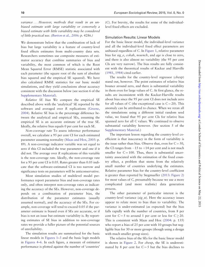
For the basic linear model, the individual-level variance

and all the individual-level fixed effect parameters are

unbiased regardless of C. In Figure 1, relative parameter

bias for sig_e, cohab, nownch, and age is close to zero,

and there is also almost no variability (the 95 per cent

CIs are very narrow). The bias results are fully consist-

ent with the theoretical results of Kackar and Harville

(1981, 1984) cited earlier.

The results for the country-level regressor (chexp)

stand out, however. The point estimates of relative bias

bounce around zero, and there is substantial variability

in them even for large values of C. At first glance, the re-

sults are inconsistent with the Kackar-Harville results

about bias since the 95 per cent CI does not include zero

for all values of C (the exceptional case is C¼20). This

anomaly can be attributed to chance. When we reran all

the simulations using a different initial random seed

value, we found that 95 per cent CIs for relative bias

spanned zero for all C values. We continued to observe

substantial variability however. (See section 5 of the

Supplementary Material.)

The important lesson regarding the country-level co-

efficient is that inaccuracy in the form of variability is

the issue rather than bias. Observe that, even for C¼50,

the CI ranges from �15 to þ14 per cent and is not much

smaller for C¼ 100. Thus, there is substantial uncer-

tainty associated with the estimation of the fixed coun-

try effect, a problem that stems from the relatively

small number of countries underlying the estimates.

Relative parameter bias for the country-level coefficient

is greater than reported by Stegmueller (2013: Figure 2)

for most values of C, presumably because we use a more

complicated (and more realistic) data generation

process.

The other parameter of particular interest is the

country-level variance (sig_u). Here the accuracy issues

appear to relate more to bias than to variability. The

variance is under-estimated (as expected) but the bias

falls rapidly with the number of countries, from 8 per

cent for C¼5 to around 1 per cent or less for C�20.

This is consistent with Maas and Hox (2004: p. 135)

who report a bias of 25 per cent with 10 groups but neg-

ligible bias for 30 or more groups (though using a design

with much smaller group sizes).

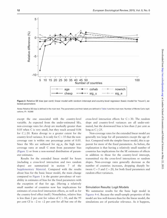
The relative bias of the SEs for the basic linear model

is shown in Figure 2. For chexp, the SE is underesti-

mated by 8 per cent for C¼ 5 but the bias declines to





Dow

nloaded from




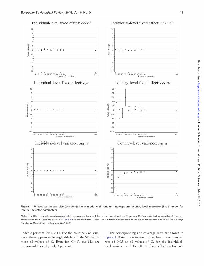
under 2 per cent for C� 15. For the country-level vari-

ance, there appears to be negligible bias in the SEs for al-

most all values of C. Even for C¼ 5, the SEs are

downward biased by only 3 per cent.

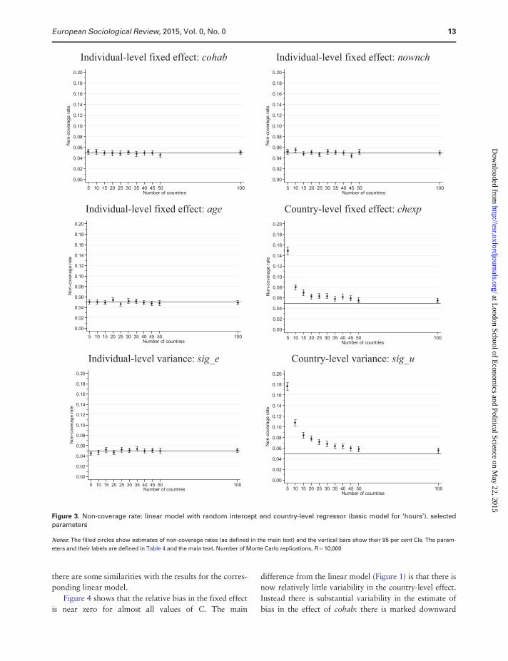
The corresponding non-coverage rates are shown in

Figure 3. Rates are estimated to be close to the nominal

rate of 0.05 at all values of C, for the individual-

level variance and for all the fixed effect coefficients

Individual-level fixed effect: cohab Individual-level fixed effect: nownch

Individual-level fixed effect: age Country-level fixed effect: chexp

Individual-level variance: sig_e Country-level variance: sig_u

-10

-8

-6

-4

-2

0

2

4

6

8

10R

elat

ive

bias

(%)

5 10 15 20 25 30 35 40 45 50 100Number of countries

-10

-8

-6

-4

-2

0

2

4

6

8

10

Rel

ativ

e bi

as (%

)


-10

-8

-6

-4

-2

0

2

4

6

8

10

Rel

ativ

e bi

as (%

)


-100

-80

-60

-40

-20

0

20

40

60

80

100

Rel

ativ

e bi

as (%

)


-10

-8

-6

-4

-2

0

2

4

6

8

10

Rel

ativ

e bi

as (%

)


-10

-8

-6

-4

-2

0

2

4

6

8

10

Rel

ativ

e bi

as (%

)


Figure 1. Relative parameter bias (per cent): linear model with random intercept and country-level regressor (basic model for

‘hours’), selected parameters

Notes: The filled circles show estimates of relative parameter bias, and the vertical bars show their 95 per cent CIs (see main text for definitions). The par-

ameters and their labels are defined in Table 4 and the main text. Observe the different vertical scale in the graph for country-level fixed effect chexp.

Number of Monte Carlo replications, R¼10,000





Dow

nloaded from


except the one associated with the country-level

variable. As expected from the under-estimated SEs,

non-coverage rates for chexp are markedly greater than

0.05 when C is very small, but they reach around 0.06

for C�20. Rates diverge to a greater extent for the

country-level variance. It is only for C> 35 that the non-

coverage rate is within one percentage point of 0.05.

Since the SEs are unbiased for sig_u, the high non-

coverage rates at small C stem from parameter bias

(Figure 1) or from a non-normal distribution of param-

eter estimates.

Results for the extended linear model for hours

(including a cross-level interaction and two random

slopes) are summarized in section 7 of the

Supplementary Material. Compared with the results

about bias for the basic linear model, the main change

compared to Figure 1 is the greater prevalence of vari-

ability in estimates of bias for the fixed parameters with

the exception of that for age. (Having a relatively

small number of countries now has implications for

estimates of cross-level interaction effects, as well as for

the country-level effect itself.) Nonetheless, relative bias

is less than 2 per cent for values of C> 10, and the 95

per cent CI is �2 to þ2 per cent for all but one of the

cross-level interaction effects for C> 30. The random

slope and country-level variances are all under-esti-

mated, but the downward bias is less than 2 per cent as

long as C� 25.

Non-coverage rates for the extended linear model are

generally too large for all parameters except the age ef-

fect. Compared with the simpler linear model, this is ap-

parent for more of the fixed parameters. As before, the

explanation is that having a relatively small number of

countries has implications for the SE estimates of effects

in addition to those for the country-level intercept,

transmitted via the cross-level interactions or random

slopes. Non-coverage rates generally decrease as the

number of countries increases, dropping sharply be-

tween C¼5 and C¼20, for both fixed parameters and

random effect variances.

Simulation Results: Logit Models

We summarize results for the basic logit model in

Figures 4–6. Because the small-sample properties of this

model are less well-known than for the linear model, the

simulations are of particular relevance. As it happens,

-10

-5

0

5

Rel

ativ

e di

ffere

nce

(%)


age cohab nownchchexp sig_u sig_e

Figure 2. Relative SE bias (per cent): linear model with random intercept and country-level regressor (basic model for ‘hours’), se-

lected parameters

Notes: Relative SE bias is defined in the main text. The parameters and their labels are defined in Table 4 and the main text. Number of Monte Carlo repli-

cations, R¼10,000





Dow

nloaded from



there are some similarities with the results for the corres-

ponding linear model.

Figure 4 shows that the relative bias in the fixed effect

is near zero for almost all values of C. The main

difference from the linear model (Figure 1) is that there is

now relatively little variability in the country-level effect.

Instead there is substantial variability in the estimate of

bias in the effect of cohab: there is marked downward



Individual-level variance: sig_e Country-level variance: sig_u

0.00

0.02

0.04

0.06

0.08

0.10

0.12

0.14

0.16

0.18

0.20N

on-c

over

age

rate


0.00

0.02

0.04

0.06

0.08

0.10

0.12

0.14

0.16

0.18

0.20

Non

-cov

erag

e ra

te


0.00

0.02

0.04

0.06

0.08

0.10

0.12

0.14

0.16

0.18

0.20

Non

-cov

erag

e ra

te


0.00

0.02

0.04

0.06

0.08

0.10

0.12

0.14

0.16

0.18

0.20

Non

-cov

erag

e ra

te


0.00

0.02

0.04

0.06

0.08

0.10

0.12

0.14

0.16

0.18

0.20

Non

-cov

erag

e ra

te


0.00

0.02

0.04

0.06

0.08

0.10

0.12

0.14

0.16

0.18

0.20

Non

-cov

erag

e ra

te


Figure 3. Non-coverage rate: linear model with random intercept and country-level regressor (basic model for ‘hours’), selected

parameters

Notes: The filled circles show estimates of non-coverage rates (as defined in the main text) and the vertical bars show their 95 per cent CIs. The param-

eters and their labels are defined in Table 4 and the main text. Number of Monte Carlo replications, R¼10,000





Dow

nloaded from


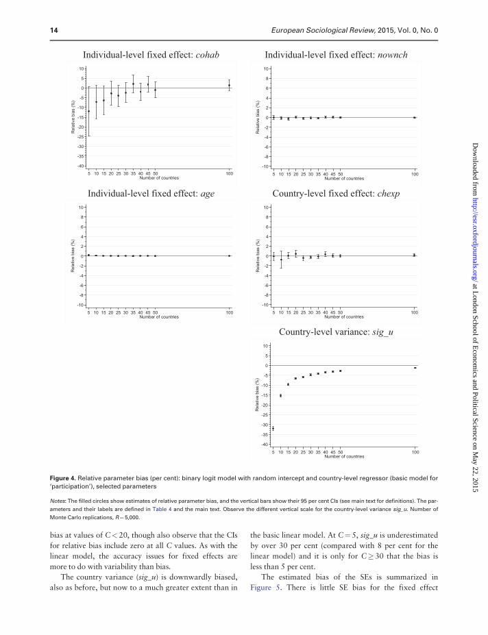
bias at values of C< 20, though also observe that the CIs

for relative bias include zero at all C values. As with the

linear model, the accuracy issues for fixed effects are

more to do with variability than bias.

The country variance (sig_u) is downwardly biased,

also as before, but now to a much greater extent than in

the basic linear model. At C¼ 5, sig_u is underestimated

by over 30 per cent (compared with 8 per cent for the

linear model) and it is only for C�30 that the bias is

less than 5 per cent.

The estimated bias of the SEs is summarized in

Figure 5. There is little SE bias for the fixed effect



Country-level variance: sig_u

-40

-35

-30

-25

-20

-15

-10

-5

0

5

10R

elat

ive

bias

(%)


-10

-8

-6

-4

-2

0

2

4

6

8

10

Rel

ativ

e bi

as (%

)


-10

-8

-6

-4

-2

0

2

4

6

8

10

Rel

ativ

e bi

as (%

)


-10

-8

-6

-4

-2

0

2

4

6

8

10

Rel

ativ

e bi

as (%

)


-40

-35

-30

-25

-20

-15

-10

-5

0

5

10

Rel

ativ

e bi

as (%

)


Figure 4. Relative parameter bias (per cent): binary logit model with random intercept and country-level regressor (basic model for

‘participation’), selected parameters

Notes: The filled circles show estimates of relative parameter bias, and the vertical bars show their 95 per cent CIs (see main text for definitions). The par-

ameters and their labels are defined in Table 4 and the main text. Observe the different vertical scale for the country-level variance sig_u. Number of

Monte Carlo replications, R¼ 5,000.





Dow

nloaded from


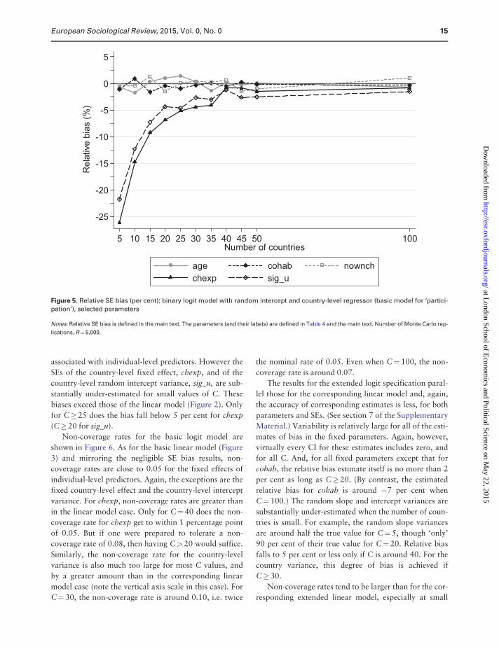
associated with individual-level predictors. However the

SEs of the country-level fixed effect, chexp, and of the

country-level random intercept variance, sig_u, are sub-

stantially under-estimated for small values of C. These

biases exceed those of the linear model (Figure 2). Only

for C�25 does the bias fall below 5 per cent for chexp

(C� 20 for sig_u).

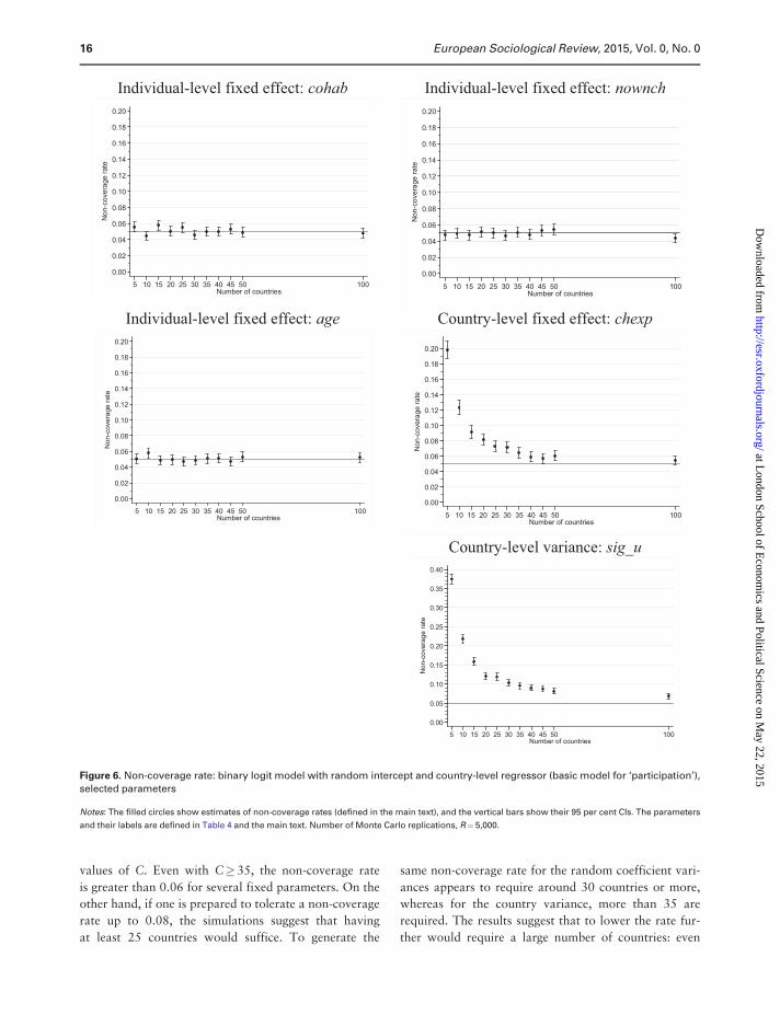
Non-coverage rates for the basic logit model are

shown in Figure 6. As for the basic linear model (Figure

3) and mirroring the negligible SE bias results, non-

coverage rates are close to 0.05 for the fixed effects of

individual-level predictors. Again, the exceptions are the

fixed country-level effect and the country-level intercept

variance. For chexp, non-coverage rates are greater than

in the linear model case. Only for C¼40 does the non-

coverage rate for chexp get to within 1 percentage point

of 0.05. But if one were prepared to tolerate a non-

coverage rate of 0.08, then having C>20 would suffice.

Similarly, the non-coverage rate for the country-level

variance is also much too large for most C values, and

by a greater amount than in the corresponding linear

model case (note the vertical axis scale in this case). For

C¼ 30, the non-coverage rate is around 0.10, i.e. twice

the nominal rate of 0.05. Even when C¼ 100, the non-

coverage rate is around 0.07.

The results for the extended logit specification paral-

lel those for the corresponding linear model and, again,

the accuracy of corresponding estimates is less, for both

parameters and SEs. (See section 7 of the Supplementary

Material.) Variability is relatively large for all of the esti-

mates of bias in the fixed parameters. Again, however,

virtually every CI for these estimates includes zero, and

for all C. And, for all fixed parameters except that for

cohab, the relative bias estimate itself is no more than 2

per cent as long as C�20. (By contrast, the estimated

relative bias for cohab is around �7 per cent when

C¼ 100.) The random slope and intercept variances are

substantially under-estimated when the number of coun-

tries is small. For example, the random slope variances

are around half the true value for C¼ 5, though ‘only’

90 per cent of their true value for C¼20. Relative bias

falls to 5 per cent or less only if C is around 40. For the

country variance, this degree of bias is achieved if

C� 30.

Non-coverage rates tend to be larger than for the cor-

responding extended linear model, especially at small

-25

-20

-15

-10

-5

0

5

Rel

ativ

e bi

as (%

)


age cohab nownchchexp sig_u

Figure 5. Relative SE bias (per cent): binary logit model with random intercept and country-level regressor (basic model for ‘partici-

pation’), selected parameters

Notes: Relative SE bias is defined in the main text. The parameters (and their labels) are defined in Table 4 and the main text. Number of Monte Carlo rep-

lications, R¼5,000.





Dow

nloaded from




values of C. Even with C� 35, the non-coverage rate

is greater than 0.06 for several fixed parameters. On the

other hand, if one is prepared to tolerate a non-coverage

rate up to 0.08, the simulations suggest that having

at least 25 countries would suffice. To generate the

same non-coverage rate for the random coefficient vari-

ances appears to require around 30 countries or more,

whereas for the country variance, more than 35 are

required. The results suggest that to lower the rate fur-

ther would require a large number of countries: even



Country-level variance: sig_u

0.00

0.02

0.04

0.06

0.08

0.10

0.12

0.14

0.16

0.18

0.20N

on-c

over

age

rate


0.00

0.02

0.04

0.06

0.08

0.10

0.12

0.14

0.16

0.18

0.20

Non

-cov

erag

e ra

te


0.00

0.02

0.04

0.06

0.08

0.10

0.12

0.14

0.16

0.18

0.20

Non

-cov

erag

e ra

te


0.00

0.02

0.04

0.06

0.08

0.10

0.12

0.14

0.16

0.18

0.20

Non

-cov

erag

e ra

te


0.00

0.05

0.10

0.15

0.20

0.25

0.30

0.35

0.40

Non

-cov

erag

e ra

te


Figure 6. Non-coverage rate: binary logit model with random intercept and country-level regressor (basic model for ‘participation’),

selected parameters

Notes: The filled circles show estimates of non-coverage rates (defined in the main text), and the vertical bars show their 95 per cent CIs. The parameters

and their labels are defined in Table 4 and the main text. Number of Monte Carlo replications, R¼5,000.





Dow

nloaded from


when C¼ 100, the non-coverage rate is greater than

0.06, for all three variances.

Lessons of the Monte Carlo Simulation Analysis

How many countries does one need for multilevel model

analysis of multi-country data to provide reliable esti-

mates? One short answer based on our simulation ana-

lysis might be: at least 25 countries for linear models

and at least 30 countries for logit models. However,

there is no simple ‘magic’ number for researchers to ap-

peal to.

For instance, the critical number of countries de-

pends on a researcher’s definition of acceptable accur-

acy. We have used as reference points a relative bias of 0

per cent and a non-coverage rate of 0.05, but fewer

countries might be sufficient if one is content to be

merely fairly ‘close’ to these ideals, or more if the refer-

ence points are applied strictly. It is the responsibility of

researchers to be clear about what counts as acceptable

accuracy.

Crude rules of thumb should not be applied blindly,

in any case. We have demonstrated that the minimum

number of countries required depends on what model is

being estimated and which effects the researcher is pri-

marily interested in.

At one extreme, it is well known that for a linear

model, REML produces unbiased estimates of the effects

of fixed individual-level covariates and our simulations

confirm this. But our simulations also show that unbias-

edness may coincide with a substantial degree of estimate

inaccuracy owing to variability, particularly for effects

associated with country-level factors (country effects and

cross-level interaction effects), reflecting the small number

of countries relative to the number of individuals per

country. Country-level variances are also prone to under-

estimation and reported SEs for them lead to unreliable

inference. In addition, our extended model results suggest

that introducing more country effects in the form of

cross-level interactions or country-level random slopes

can lead to additional reliability problems. There is also

the more general point that our results refer to data sets

with very large numbers of individuals per country. If

there are substantially fewer level-1 observations per

level-2 cluster, for example, the critical number of obser-

vations is likely to differ.

Put differently, we recommend that researchers fit-

ting relatively complicated models should seek data sets

with numbers of countries greater than those cited above

if they wish to be confident of having reliable results. By

‘relatively complicated models’ we mean models with

multiple country-level or cross-level fixed effects (the

greater the number, the fewer the effective degrees of

freedom) and, more generally, models that differ from

the ‘basic’ specifications that we have focused on.

More positively, we have shown that non-coverage

rates for fixed effects in linear models are relatively

good as long as the number of countries is greater than

around 25. With this number of countries, linear model

estimates of random effect variances and their SEs also

appear to be accurate to an extent that may satisfy many

practising researchers.

Our simulation results for the binary logit models re-

garding relative bias and non-coverage have parallels

with those for the corresponding linear models. The pri-

mary difference between models is that a greater number

of countries are necessary for logit models to generate the

same degree of accuracy in parameter estimates and SEs,

other things being equal. In particular for random coeffi-

cient variances (if specified) and especially the country-

level variance, at least 30–35 countries may be required

to derive accurate estimates—which is more countries

than is usually available (see Table 1). Our recommenda-

tions above concerning ‘relatively complicated models’

have particular force in the case of non-linear models.

An additional warning concerning non-linear multi-

level models in general and the binary logit mixed model

in particular is that the estimator used for maximization

also matters. We have used ML with adaptive Gaussian

quadrature. This has been found to produce more accur-

ate estimates than penalized quasi-likelihood both with

data structures different from ours (Rodriguez and

Goldman, 2001; Callens and Croux, 2005; Pinheiro and

Chao, 2006; Austin, 2010) and also with the same data

structure as used in this article (Jenkins, 2013). Other re-

searchers have shown that Bayesian estimation methods

using Markov chain Monte Carlo methods also perform

better than ML when the number of groups (‘countries’)

is small. See Austin (2010), Browne and Draper (2000,

2006), and Stegmueller (2013).

Summary and Conclusions

When there are few countries in a multi-country data

set, there is little information with which to estimate

country effects, whether these effects refer to the fixed

parameters on country-level predictors or the variances

of random country intercepts. Multilevel model users

need to be cautious in the claims they make about coun-

try effects of either type.

Our Monte Carlo simulations suggest that users re-

quire 25 countries for linear models and 30 countries for

logit models at the very minimum, and most likely more

for models with a specification other than a relatively





Dow

nloaded from


basic one. Otherwise, estimates of country-level fixed par-

ameters are likely to be estimated imprecisely and this

will not be adequately reflected in test statistics reported

by commonly used software: users will conclude too often

that a country effect exists when it does not. Country ran-

dom variances will be biased downwards and have CIs

that are too narrow. The only estimates that are un-

affected by having a small number of countries are the

fixed parameters on individual-level predictors (the num-

ber of individuals per country is typically large): provided

there is not also a random component attached to the

slope, these parameters are estimated without bias and

with the correct SEs (and non-coverage rate).

Since the critical number of countries required for reli-

able estimation of country effects is larger than the num-

ber of countries in many existing data sets, what can

analysts do in the small-C case (in addition to being cau-

tious in their claims)? We recommend three strategies.

One is to supplement regression-based modelling

with more descriptive analysis of measured country dif-

ferences. We referred earlier in the discussion of the

two-step approach to exploratory data analysis based

on visualization of country differences. On this, see

Bowers and Drake (2005) and also the examples in sec-

tion 8 of this article’s Supplementary Material. The two-

step approach may reveal features of the data, such as

country groupings, that are worthy of further investiga-

tion; or could highlight outliers that have an undue

influence owing to the small number of countries—

perhaps prompting a more systematic examination using

jackknifing and influence statistics (Van der Meer, Te

Grotenhuis and Pelzer, 2010).

A second strategy is to use methods that are more ro-

bust to small numbers of countries, as mentioned in sec-

tion 3. These include small sample corrections, such as

those available in SAS and R for linear models, and

bootstrapping. However, we note that some of these

techniques require specialized knowledge and are not

routinely available in the software packages most com-

monly used by social scientists, and they are not applic-

able to all parameters of interest.

A third strategy would be to move beyond the clas-

sical (‘frequentist’) statistical framework used by most

applied social science researchers and to make greater

use of Bayesian methods of estimation and inference, as

there is some evidence that they perform better in the

small-C case (see section 4). In the Bayesian paradigm,

the researcher specifies a ‘prior distribution’ for the

model parameters that embodies a belief about their

plausible range of values. Estimation produces a ‘poster-

ior distribution’ of parameters that reflects both the

observed data and the priors. It is because Bayesian

inferences account for the uncertainty in the parameters

across their plausible range that they are more reliable

than classical methods when level-2 (country) sample

sizes are small (Raudenbush and Bryk, 2002: chapter

13). However, this superior performance of Bayesian es-

timation relies on the priors being correctly specified.

With a small number of countries, the prior may have a

large influence on the posterior and so it is essential to

check the sensitivity of results to alternative priors

(Seltzer, Wong and Bryk, 1996).

There is a general challenge to a prescription of more

widespread use of Bayesian methods for multilevel mod-

elling, and that is that such methods require statistical

expertise beyond that of most applied social science re-

searchers, as well as specialist software (or software

with which such researchers are unfamiliar). It is appar-

ently not enough that there are already short introduc-

tions in general multilevel modelling textbooks (for

example, Raudenbush and Bryk, 2002: chapter 13;

Brown and Prescott, 2006: section 2.3), review articles

such as Draper (2008), and a number of textbooks

focusing on Bayesian multilevel modelling such as

Gelman et al. (2013) or Gill (2008).

In addition to these three strategies for analysis of

country effects using hierarchical multi-country data

sets, there remains a need for detailed consideration of

the workings of national institutions and policies.

Multilevel modelling methods are no panacea.

Acknowledgements

For assistance, comments, and suggestions, the authors thank

Bjaarte Aagnes, William Buchanan, Mike Kenward, Henning

Lohmann, Joerg Luedicke, Matthias Parey, Steve Pudney, Fiona

Steele, Jay Verkuilen, our ALiCE project collaborators, and

seminar participants at Assisi, Essex, IFS, IoE, LSE, LSHTM,

Oxford, and Sheffield. We are also grateful to the Editor and

four anonymous referees for their detailed comments.

Funding

This research was supported by funding from the UK Economic

and Social Research Council for the Analysing Life Changes in

Europe project (RES-062-23-1455). Core funding from the

ESRC (RES-518-28-001) and the University of Essex for the

Research Centre on Micro-Social Change at ISER is also

acknowledged.

References

Angrist, J. D. and Pischke, J.-S. (2009). Mostly Harmless

Econometrics: An Empiricist’s Companion. Princeton NJ:

Princeton University Press.





Dow

nloaded from



Austin, P. C. (2010). Estimating multilevel logistic regression

models when the number of clusters is low: a comparison of

different statistical software procedures. International Journal

of Biostatistics, 6, article 16.

Bell, B. A. et al. (2014). How low can you go? An investigation

of the influence of sample size and model complexity on

point and interval estimates in two-level linear models.

Methodology 10, 1–11.

Borjas, G. J. and Sueyoshi, G. T. (1994). A two-stage estimator

for probit models with structural group effects. Journal of

Econometrics, 64, 165–182.

Bowers, J. and Drake, K. W. (2005). EDA for HLM: visualiza-

tion when probabilistic inference fails. Political Analysis, 13,

301–326.

Brown, H. and Prescott, R. (2006). Applied Mixed Models in

Medicine, 2nd edn. New York: Wiley.

Browne, W. C. and Draper, D. (2000). Implementation and per-

formance issues in Bayesian and likelihood fitting of multilevel

models. Computational Statistics, 15, 391–420.

Browne, W. J. and Draper, D. (2006). A comparison of Bayesian

and likelihood-based methods for fitting multilevel models.

Bayesian Analysis, 1, 473–514.

Burton, A. et al. (2006). The design of simulation studies in med-

ical statistics. Statistics in Medicine, 25, 4279–4292.

Callens, M. and Croux, C. (2005). Performance of likelihood-

based estimation methods for multilevel binary regression

models. Journal of Statistical Computation and Sumulation,

75, 1003–1017.

Cameron, C. A., Gelbach, J. B. and Miller, D. L. (2008). Bootstrap-

based improvements for inference with clustered standard errors.

Review of Economics and Statistics, 90, 414–427.

Cameron, C. A. and Miller, D. L. (2013). A practitioner’s guide

to cluster-robust inference. Unpublished paper, University of

California Davis, available from: <http://cameron.econ.ucdav

is.edu/research/Cameron_Miller_Cluster_Robust_October15

2013.pdf> [accessed 14 August 2014]. Forthcoming, Journal

of Human Resources.

Cameron, C. A. and Trivedi P. K. (2010), Microeconometrics

Using Stata, revised edition. College Station, TX: Stata Press.

Card, D. (1995). The wage curve: a review. Journal of Economic

Literature, 33, 285–299.

Carpenter, J. R., Goldstein, H. and Rasbash, J. (2003). A novel

bootstrap procedure for assessing the relationship between

class size and achievement. Applied Statistics, 52, 431–443.

Centre for Multilevel Modelling. (2011). Sample sizes for multi-

level models. Bristol: University of Bristol, available from:

<http://www.bristol.ac.uk/cmm/learning/multilevel-models/

samples.html> [accessed 14 August 2014].

Donald, S. G. and Lang, K. (2007). Inference with difference-in-

differences and other panel data. Review of Economics and

Statistics, 89, 221–233.

Draper, D. (2008). Bayesian multilevel analysis and MCMC. In

de Leeuw, J. and Meijer, E. (Eds.), Handbook of Multilevel

Analysis. New York: Springer, pp. 77–139.

Gelman, A. et al. (2013). Bayesian Data Analysis, 3rd ed. Boca

Raton, FL: Chapman & Hall/CRC.

Gill, J. (2008). Bayesian Methods: A Social and Behavioral

Sciences Approach, 2nd ed. Boca Raton, FL: Chapman and

Hall/CRC.

Greene, W. (2004). The behaviour of the maximum likelihood

estimator of limited dependent variable models in the presence

of fixed effects. Econometrics Journal, 7, 98–119.

Hanushek, E. A. (1974). Efficient estimators for regressing re-

gression coefficients. American Statistician, 28, 66–67.

Hox, J. J. (2010). Multilevel Analysis: Techniques and

Applications, 2nd ed. London: Routledge.

Jenkins, S. P. (2013). A Monte-Carlo analysis of multilevel bin-

ary logit model estimator performance. Presentation at the

Stata User Group Meeting, London, 13 September, available

from: <http://repec.org/usug2013/jenkins.uk13.pdf> [ac-

cessed 14 August 2014).

Jusko, K. L. and Shively, W. P. (2005). A two-step strategy for

the analysis of cross-national public opinion data. Political

Analysis, 13, 327–344.

Kackar, R. H. and Harville, D. A. (1981). Unbiasedness of two-

stage estimation and prediction procedures for mixed linear

models. Communications in Statistics: Theory and Methods,

13, 1249–1261.

Kackar, R. H. and Harville, D. A. (1984). Approximations for

standard errors of estimators of fixed and random effects in

mixed linear models. Journal of the American Statistical

Association, 79, 853–862.

Kedar, O. and Shively, W. P. (2005). Introduction to the special

issue. Political Analysis, 13, 297–300.

Kenward, M. G. and Roger, J. H. (1997). Small sample inference

for fixed effects from restricted maximum likelihood.

Biometrics, 53, 983–997.

Kenward, M. G. and Roger, J. H. (2009). An improved approxi-

mation to the precision of fixed effects from restricted max-

imum likelihood. Computational Statistics and Data Analysis,

53, 2583–2595.

Maas, C. J. M. and Hox, J. J. (2004). Robustness issues in multi-

level regression analysis. Statistica Neerlandica, 58, 127–137.

Maas, C. J. M. and Hox, J. J. (2005). Sufficient sample sizes for

multilevel modelling. Methodology, 1, 86–92.

Moineddin, R., Matheson, F. I. and Glazier, R. H. (2007).

A simulation study of sample size in multilevel regression

models. BMC Medical Research Methodology, 7, article 34.

Molenberghs, G. and Verbeke, G. (2005). Models for Discrete

Longitudinal Data. New York: Springer.

Moulton, B. R. (1986). Random group effects and the precision of

regression estimates. Journal of Econometrics, 32, 385–397.

Neuhaus, J. M., Kalbfleisch, J. D. and Hauck, W. W. (1991).

A comparison of cluster-specific and population-averaged

approaches to analysing correlated binary data. International

Statistical Review, 59, 25–35.

Paccagnella, O. (2011). Sample size and accuracy of estimates in

multilevel models. Methodology, 7, 111–120.

Pinheiro, J. C. and Chao, E. C. (2006). Efficient Laplacian and

adaptive quadrature algorithms for multilevel generalized lin-

ear mixed models. Journal of Computational and Graphical

Statistics, 15, 58–81.





Dow

nloaded from

http://cameron.econ.ucdavis.edu/research/Cameron_Miller_Cluster_Robust_October152013.pdf



http://www.bristol.ac.uk/cmm/learning/multilevel-models/samples.html

http://www.bristol.ac.uk/cmm/learning/multilevel-models/samples.html

http://repec.org/usug2013/jenkins.uk13.pdf


Raudenbush, S. W. and Bryk, A. S. (2002). Hierarchical Linear

Models: Applications and Data Analysis Methods, 2nd ed.

Thousand Oaks, CA: Sage Publications.

Raudenbush S. W. et al. (2004). HLM 6: Hierarchical Linear

and Nonlinear Modeling. Lincolnwood, IL: Scientific

Software International.

Rodriguez, G. and Goldman, N. (2001). Improved estimation pro-

cedures for multilevel models with binary response: case study.

Journal of the Royal Statistical Society, Series A, 164, 339–355.

Saxonhouse, G. R. (1976). Estimated parameters as dependent

variables. American Economic Review, 66, 178–183.

Seltzer, M. H., Wong, W. H. and Bryk, A. S. (1996). Bayesian

analysis in applications of hierarchical models: issues and

methods. Journal of Educational and Behavioral Statistics, 21,

131–167.

Snijders, T. A. B. and Bosker, R. (2012). Multilevel Analysis: An

Introduction to Basic and Advanced Multilevel Modeling,

2nd ed. Thousand Oaks, CA: Sage Publications Ltd.

StataCorp (2011). Stata Statistical Software, Release 12. College

Station, TX: StataCorp.

Stegmueller, D. (2013). How many countries do you need for

multilevel modeling? A comparison of Bayesian and frequent-

ist approaches. American Journal of Political Science, 57,

748–761.

Van der Meer, T., Te Grotenhuis, M. and Pelzer, B.

(2010). Influential cases in multilevel modeling: a meth-

odological comment. American Sociological Review, 75,

173–178.

Wooldridge, J. (2010). Econometric Analysis of Cross Section

and Panel Data, 2nd edn. Cambridge MA: MIT Press.





Dow

nloaded from


mark l. bryan and stephen p. jenkins multilevel modelling...

Documents