Marine guided-waves: Applications and filtering using physical modeling dataJiannan Wang1, Robert Stewart1, Nikolay Dyaur1, University of Houston,and Lee Bell2, Geokinetics Inc.

SUMMARY

Guided seismic waves in the water column can be energeticevents, especially at shallow depths. This paper investigatesguided-wave properties, their use, and filtering with the helpof physical modeling experiments. We investigate how dif-ferent parameters (water depth, density of the seafloor, andboth P-wave and shear-wave velocity of the seafloor) affectthe guided-wave properties. A number of physical model-ing experiments, at the ultrasonic surveying facilities of AlliedGeophysical Laboratories (AGL), are conducted. The physicalmodeling data fit theoretical calculations very well. For a hor-izontal or slightly dipping seafloor, extracting the shear-wavevelocity from guided-waves with a curve-fitting method is ac-curately achieved. Both theoretical analysis and physical mod-eling indicate that guided-waves obscure reflection data, whichmakes removing guided-waves necessary. Because the normalmodes of guided-waves are less obvious in the f − k domain,we design a dispersion curve f ilter in the phase velocity andfrequency domain (v− f domain). The filter is tested on thephysical modeling data. The results show enhanced reflectionsand attenuated guided-waves, which can benefit further pro-cessing and interpretation.

INTRODUCTION

Guided-waves are commonly found in seismic data from shal-low water environments. With their relatively strong ampli-tudes, they can obscure the reflections from deeper targets.Note that these guided-waves interact with the seabed and there-fore are sensitive to the shear-wave velocity of the subsurfacematerial. (Klein et al., 2005). So, studying guided-waves mayalso benefit ocean-bottom seismic processing and interpreta-tion.

In this paper, we first study the influence of different waterdepth and physical properties (density, P-wave and shear-wavevelocity) in the marine environment on the dispersive spectra.Then, similar to the MASW method developed by Park et al.(1998), we extract some of the physical properties from thedispersive spectrum of the guided-waves. Finally, we designa dispersion curve f ilter in the phase velocity and frequencydomain to attenuate the guided-waves.

DISPERSION PROPERTIES

The dispersion equation of guided-waves in a layered modelwas first given by Pekeris (1945) with the assumption that alllayers are liquid. Press and Ewing (1950) extended Pekeris’development to an elastic sea-bottom. The dispersive equation

is:

tan [knH√

c2/v21−1− (m−1)π] =

ρ2

ρ1

β 42

c4

√c2/v2

1−1√1− c2/α2

2

·[4√

1− c2/α22

√1− c2/β 2

2 − (2− c2/β 22 )

2], (1)

where H is the water column thickness, ρ1 and ρ2 are the den-sity of water and seafloor, respectively, kn is the wavenumberof nth mode, v1 is velocity in water, α2 is the P wave velocityof seafloor, β2 is the S wave velocity of the seafloor, c is theguided-wave phase velocity.

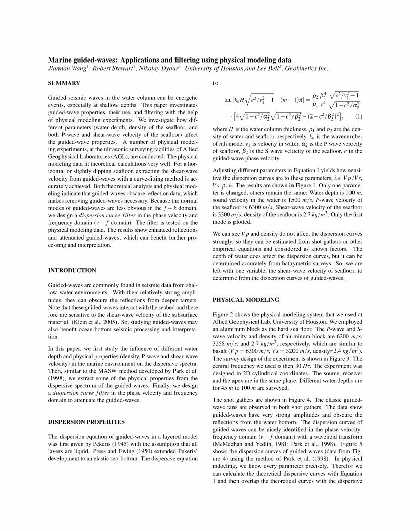
Adjusting different parameters in Equation 1 yields how sensi-tive the dispersion curves are to these parameters, i.e. V p/V s,V s, ρ , h. The results are shown in Figure 1. Only one parame-ter is changed, others remain the same: Water depth is 100 m,sound velocity in the water is 1500 m/s, P-wave velocity ofthe seafloor is 6300 m/s, Shear-wave velocity of the seaflooris 3300 m/s, density of the seafloor is 2.7 kg/m3. Only the firstmode is plotted.

We can see V p and density do not affect the dispersion curvesstrongly, so they can be estimated from shot gathers or otherempirical equations and considered as known factors. Thedepth of water does affect the dispersion curves, but it can bedetermined accurately from bathymetric surveys. So, we areleft with one variable, the shear-wave velocity of seafloor, todetermine from the dispersion curves of guided-waves.

PHYSICAL MODELING

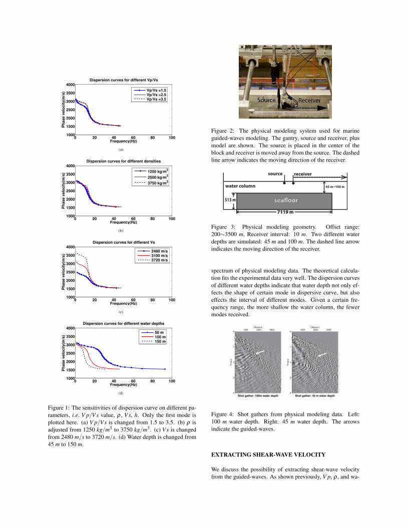
Figure 2 shows the physical modeling system that we used atAllied Geophysical Lab, University of Houston. We employedan aluminum block as the hard sea floor. The P-wave and S-wave velocity and density of aluminum block are 6200 m/s,3258 m/s, and 2.7 kg/m3, respectively, which are similar tobasalt (V p = 6300 m/s, V s = 3200 m/s, density=2.4 kg/m3).The survey design of the experiment is shown in Figure 3. Thecentral frequency we used is then 30 Hz. The experiment wasdesigned in 2D cylindrical coordinates. The source, receiverand the apex are in the same plane. Different water depths arefor 45 m to 100 m are surveyed.

The shot gathers are shown in Figure 4. The classic guided-wave fans are observed in both shot gathers. The data showguided-waves have very strong amplitudes and obscure thereflections from the water bottom. The dispersion curves ofguided-waves can be nicely identified in the phase velocity-frequency domain (v− f domain) with a wavefield transform(McMechan and Yedlin, 1981; Park et al., 1998). Figure 5shows the dispersion curves of guided-waves (data from Fig-ure 4) using the method of Park et al. (1998). In physicalmdoeling, we know every parameter precisely. Therefor wecan calculate the theoretical dispersive curves with Equation1 and then overlap the theoretical curves with the dispersive

0 20 40 60 80 1001000

1500

2000

2500

3000

3500

4000

Frequency(Hz)

Ph

as

e v

elo

cit

y(m

/s)

Dispersion curves for different Vp/Vs

Vp/Vs =1.5Vp/Vs =2.5Vp/Vs =3.5

(a)

0 20 40 60 80 1001000

1500

2000

2500

3000

3500

4000

Frequency(Hz)

Ph

as

e v

elo

cit

y(m

/s)

Dispersion curves for different densities

1250 kg/m3

2500 kg/m3

3750 kg/m3

(b)

0 20 40 60 80 1001000

1500

2000

2500

3000

3500

4000

Frequency(Hz)

Ph

as

e v

elo

cit

y(m

/s)

Dispersion curves for different Vs

2480 m/s3100 m/s3720 m/s

(c)

0 20 40 60 80 1001000

1500

2000

2500

3000

3500

4000

Frequency(Hz)

Ph

as

e v

elo

cit

y(m

/s)

Dispersion curves for different water depths

50 m100 m150 m

(d)

Figure 1: The sensitivities of dispersion curve on different pa-rameters, i.e. V p/V s value, ρ , V s, h. Only the first mode isplotted here. (a) V p/V s is changed from 1.5 to 3.5. (b) ρ isadjusted from 1250 kg/m3 to 3750 kg/m3. (c) V s is changedfrom 2480 m/s to 3720 m/s. (d) Water depth is changed from45 m to 150 m.

Figure 2: The physical modeling system used for marineguided-waves modeling. The gantry, source and receiver, plusmodel are shown. The source is placed in the center of theblock and receiver is moved away from the source. The dashedline arrow indicates the moving direction of the receiver.

45 m~100 m

sea!oor

7119 m

source receiver

513 m

water column

Figure 3: Physical modeling geometry. Offset range:200∼3500 m, Receiver interval: 10 m. Two different waterdepths are simulated: 45 m and 100 m. The dashed line arrowindicates the moving direction of the receiver.

spectrum of physical modeling data. The theoretical calcula-tion fits the experimental data very well. The dispersion curvesof different water depths indicate that water depth not only ef-fects the shape of certain mode in dispersive curve, but alsoeffects the interval of different modes. Given a certain fre-quency range, the more shallow the water column, the fewermodes received.

0

1

2

3

4

Tim

e(s

)

1000 2000 3000Offset(m)

Shot gather: 45 m water depth

0

1

2

3

4

Tim

e(s

)

1000 2000 3000Offset(m)

Shot gather: 100m water depth

Figure 4: Shot gathers from physical modeling data. Left:100 m water depth. Right: 45 m water depth. The arrowsindicate the guided-waves.

EXTRACTING SHEAR-WAVE VELOCITY

We discuss the possibility of extracting shear-wave velocityfrom the guided-waves. As shown previously, V p, ρ , and wa-

Water depth: 100 m

Frequency(Hz)

Ph

as

e v

elo

cit

y(m

/s)

0 20 40 60 80 1001000

2000

3000

4000

(a)

Water depth: 45 m

Frequency(Hz)

Ph

as

e v

elo

cit

y(m

/s)

0 20 40 60 80 1001000

2000

3000

4000

(b)

Figure 5: Dispersion plots for different water depths overlyinga flat seafloor. The blue curves are the theoretical calculation.(a) 100 m water depth. (b) 45 m water depth.

ter depth can be considered as know factors, thus shear-wavevelocity is the only one unknown parameter in the dispersionequation. Extracting the shear-wave velocity of seafloor fromguided-waves can be cast as least-squares problem by mini-mizing the residual between the dispersion curves from thedata and a predicted dispersion curves from the shear-wavevelocity (Levenberg, 1944; Marquardt, 1963). We solve thisproblem iteratively by finding V s such that:

minVs‖F(Vs,cdata)−Fdata‖2

2 =

minVs

∑i (F(Vs,cdatai)−Fdatai)

2, (2)

where cdata phase velocity corresponding to certain frequencyfrom the data, Fdata is the observed dispersion curves, andF(Vs,cdata) is the predict dispersion curves from cdata and es-timated Vs.

The Jacobian matrix is calculated with the finite differencemethod (Gavin, 2011). The Levenberg-Marquardt method cansolves this problem efficiently given a good estimated initialshear-wave velocity. However, the dispersive spectra can some-times be noisy, making the estimation of initial shear-wave ve-locity less accurate. To achieve a more rapid convergence, weuse the trust-region-reflective method (Coleman and Li, 1994,1996a,b), which is similar to Levenberg-Marquardt method,except that the bound is updated from iteration to iteration(Yuan, 2000).

Figure 6 is the cure-fitting results with the data from Figure 5.In Figure 6(a) (100 m water depth), we picked first five modesas input data. In Figure 6(b) (45 m water depth), only first three

modes are picked because of the weak amplitude in highermodes.

0 20 40 60 80 1001000

1500

2000

2500

3000

3500

4000

Frequency (Hz)

Ph

as

e v

elo

cit

y (

m/s

)

First 5 modes, water depth = 100 m

Extracting result: Vs = 3157 m/s

(a)

0 20 40 60 80 1001000

1500

2000

2500

3000

3500

4000

Frequency (Hz)

Ph

as

e v

elo

cit

y (

m/s

)

First 3 modes, water depth = 45 m

Extracting result: Vs = 3181 m/s

(b)

Figure 6: Curve-fitting and shear-wave velocity extraction re-sult. (a) 100 m water depth. (b) 45 m water depth. The dotsare picked from physical modeling data from two experimentswith different water depths. The solid curves are final calcu-lated dispersion curves.

The lab measurement of shear-wave velocity of seafloor (fromdirect transmission measurements) is V s= 3158±56 m/s. Thecurve-fitting of physical modeling data yield 3157 m/s (100 mwater depth) and 3181 m/s (50 m water depth). Consideringthe error of the lab measurement, the extracted result from theguided-waves is reasonable.

DISPERSION CURVE FILTER

From the above discussion, we can see that the normal modesof the guided-waves have significant influence on marine seis-mic data. After parameters estimation from the guided-waves,their removal is the goal. The f − k filter is a workhorse in at-tenuating dipping noise. To identify the guided-wave signaturein the f − k spectrum, we transform the theoretical calculationof dispersion curves of only the guided-waves (only the nor-mal modes) and the full spectrum (both the normal modes andthe leaky modes). Figure 7(a) shows the results. In the lowfrequency range, all events overlaps together. The differencebetween the normal mode spectrum and the full spectrum issmall. Some of the normal modes even overlap with the leakymodes. As mentioned before, the real part of the leaky modesis the Scholte waves. It is difficult to separate the guided-wavesin the f − k spectrum from the Scholte waves. The convertedreflections and refractions cut through the normal modes andleaky modes. So, for multicomponent seismic data, attenu-ating guided-waves without damaging converted wave signal

in f − k domain would be very challenging. Transferring ourphysical modeling data (100 m water depth) into f −k domain(the left figure in Figure 7(b)), with the blurring effect in thereal data, we find the guided-waves, different reflections, andthe refractions superpose, which makes the isolation of guided-waves in f − k domain even more difficult.

−0.5 0 0.50

20

40

Wavenumber(k)

Fre

qu

en

cy(H

z)

(a)

0

20

40

Frequency(Hz)

-0.5 0Wavenumber(k)

0.5

(b)

Figure 7: Transferring the dispersion curves into the f − k do-main. (a) the normal modes and leaky modes, blue curves arenormal modes, red curves are leaky modes, black dashed linesare P−wave and converted wave refractions, green curves areP−wave and converted wave reflections. (b) f −k spectrum ofphysical modeling data (100 m water depth).

Because the f − k filter is unlikely be completely satisfactory,we seek a new way to filter. The normal modes and leakymodes are well separated in the v− f domain (Pekeris, 1945;Press and Ewing, 1950). Moreover, different modes of normalmodes are also well separated. We design a filter in the v− fdomain. McMechan and Yedlin (1981) developed a method oftransferring the shot gather into slowness-frequency domain(p−ω). Their method requires long offsets and wide incidentangles, which is appropriate for our marine case.

According to previous section, all the parameters can be con-sidered as known (V p, ρ , h) or well estimated (V s). So, calcu-lating the dispersion curves of guided-waves and masking dataalong these curves in the v− f domain with these curves willlargely reject the guided-waves while minimizing attenuationof other events.

To test our method, we applied this masking filter on our physi-cal modeling data set, both 100 m and 45 m water depth (Figure8). No gain enhancement is applied to the data. As we can see,the guided-waves (indicated by the arrow) are attenuated quitewell. Because the guided-waves contain considerable energyin the shot gather, after applying the dispersion curve filter, theenergy of reflection and refraction become more distinct.

CONCLUSIONS

Guided-waves can obscure reflections in marine seismic data,but they carry information about the seafloor. These guided-waves are well observed in physical modeling data. The dis-persion curves from the physical modeling data match theoret-ical calculations very well. The shape of the guided-wave dis-

0

1

2

3

4

Time(s)

1000 2000 3000Offset(m)

After filtering, water depth: 45 m

0

1

2

3

4

Time(s)

1000 2000 3000Offset(m)

Before filtering, water depth: 45 m

(a)

0

1

2

3

4

Time(s)

1000 2000 3000Offset(m)

After filtering, water depth: 100 m

0

1

2

3

4

Time(s)

1000 2000 3000Offset(m)

Before filtering, water depth: 100 m

(b)

Figure 8: Comparison between original (left) and filtered(right) shot gathers. (a) 45 m water depth. (b) 100 m waterdepth.

persion curve is largely determined by the shear-wave velocityof the seafloor and is not sensitive to other physical parameters.We are able to extract the shear-wave velocity of the seafloorfrom the guided-waves with a least-square based curve-fittingmethod. Existing filtering techniques may have difficulty sep-arating the normal modes energy from other events. We de-veloped a dispersion curve filter. The filter is tested on twophysical modeling data with different water depths. The re-sults show that this dispersion curve filter works very well andmay benefit further processing and interpretation.

ACKNOWLEDGMENTS

We would like to thank Anoop William of the Allied Geo-physical Laboratories (AGL) at University of Houston whoprovided us with substantial assistance with the experiments.Dr. Bob WiIey also with AGL helped with software develop-ment. We are grateful to Geokinetics, Houston for generouslysupporting this project. We are also grateful to Dr. SoumyaRoy formerly of the University of Houston for inspiring dis-cussions.

REFERENCES

Brekhovskikh, L. M., and O. A. Godin, 1999, Acoustics of lay-ered media ii: point sources and bounded beams: Springer,2.

Burg, K., M. Ewing, F. Press, and E. Stulken, 1951, A seismicwave guide phenomenon: Geophysics, 16, 594–612.

Burns, D., C. Cheng, and M. Toksoz, 1985, Energy parti-tioning and attenuation of guided waves in a radially lay-ered borehole: Technical report, Massachusetts Institute ofTechnology. Earth Resources Laboratory.

Coleman, T. F., and Y. Li, 1994, On the convergence ofinterior-reflective newton methods for nonlinear minimiza-tion subject to bounds: Mathematical programming, 67,189–224.

——–, 1996a, An interior trust region approach for nonlin-ear minimization subject to bounds: SIAM Journal on opti-mization, 6, 418–445.

——–, 1996b, A reflective newton method for minimizing aquadratic function subject to bounds on some of the vari-ables: SIAM Journal on Optimization, 6, 1040–1058.

Cooper, J. K., D. C. Lawton, and G. F. Margrave, 2010, Thewedge model revisited: A physical modeling experiment:Geophysics, 75, T15–T21.

Etter, P. C., 2013, Underwater acoustic modeling and simula-tion: CRC Press.

Gavin, H., 2011, The levenberg-marquardt method for non-linear least squares curve-fitting problems: Department ofCivil and Environmental Engineering, Duke University.

Katsnelson, B., V. Petnikov, and J. Lynch, 2012, Fundamentalsof shallow water acoustics: Springer.

Klein, G., T. Bohlen, F. Theilen, S. Kugler, and T. For-briger, 2005, Acquisition and inversion of dispersive seis-mic waves in shallow marine environments: Marine Geo-physical Researches, 26, 287–315.

Kuperman, W., and M. Ferla, 1985, A shallow water ex-periment to determine the source spectrum level of wind-generated noise: The Journal of the Acoustical Society ofAmerica, 77, 2067–2073.

Lansley, R. M., P. L. Eilert, D. L. Nyland, et al., 1984, Surfacesources on floating ice: the flexural ice wave: Presentedat the 1984 SEG Annual Meeting, Society of ExplorationGeophysicists.

Levenberg, K., 1944, A method for the solution of certainproblems in least squares: Quarterly of applied mathemat-ics, 2, 164–168.

Liner, C. L., 2012, Elements of seismic dispersion: A some-what practical guide to frequency-dependent phenomena:Society of Exploration Geophysicists.

Marquardt, D. W., 1963, An algorithm for least-squares esti-mation of nonlinear parameters: Journal of the Society forIndustrial & Applied Mathematics, 11, 431–441.

McDonald, J. A., G. Gardner, and F. J. Hilterman, 1983, Seis-mic studies in physical modeling: IHRDC.

McMechan, G. A., and M. J. Yedlin, 1981, Analysis of disper-sive waves by wave field transformation: Geophysics, 46,869–874.

Norris, A. N., and B. K. Sinha, 1995, The speed of a wavealong a fluid/solid interface in the presence of anisotropy

and prestress: The Journal of the Acoustical Society ofAmerica, 98, 1147–1154.

Officer, C. B., and R. R. Shrock, 1958, Introduction to the the-ory of sound transmission: With application to the ocean:McGraw-Hill New York.

Park, C. B., R. D. Miller, J. Xia, et al., 1998, Ground roll asa tool to image near-surface anomaly: 68th SEG Meeting,New Orleans, USA, Expanded Abstracts, 874–877.

Pekeris, C. L., 1945, Theory of propagation of explosive soundin shallow water: Geological Society of America.

Press, F., and M. Ewing, 1950, Propagation of explosive soundin a liquid layer overlying a semi-infinite elastic solid: Geo-physics, 15, 426–446.

Stewart, R. R., N. Dyaur, B. Omoboya, J. de Figueiredo, M.Willis, and S. Sil, 2012, Physical modeling of anisotropicdomains: Ultrasonic imaging of laser-etched fractures inglass: Geophysics, 78, D11–D19.

Tolstoy, I., 1954, Dispersive properties of a fluid layer overly-ing a semi-infinite elastic solid: Bulletin of the Seismolog-ical Society of America, 44, 493–512.

Uren, N., G. Gardner, J. McDonald, et al., 1989, Zero-offsetseismic reflection surveys using an anisotropic physicalmodel: Presented at the 1989 SEG Annual Meeting, So-ciety of Exploration Geophysicists.

Yuan, Y.-x., 2000, A review of trust region algorithms for op-timization: ICIAM, 271–282.

Zhu, J., J. S. Popovics, and F. Schubert, 2004, Leaky rayleighand scholte waves at the fluid–solid interface subjected totransient point loading: The Journal of the Acoustical Soci-ety of America, 116, 2101–2110.