Mapping Poverty in Rural Papua New Guinea

John Gibson

Department of Economics University of Waikato

Gaurav Datt The World Bank

Sydney

Bryant Allen Dept of Human Geography

Australian National University

Vicky Hwang The World Bank

Sydney

R. Michael Bourke Dept of Human Geography

Australian National University

Dilip Parajuli The World Bank

Washington D. C.

August 31, 2004

Abstract In this paper, disaggregated maps of rural poverty in Papua New Guinea are created by combining information from a 1996 Household Survey with data from the 2000 Census, and from resource and agricultural mapping databases with national coverage. Predicted poverty rates are presented at Provincial, District and Local Level Government (LLG) level. Predicted poverty is highest in Sandaun Province. Existing national grants to provinces appear to be unrelated to poverty status. However, the more revealing feature of the results is the high level of within-province heterogeneity. Hence, public spending interventions that try to target poor provinces are likely to miss large numbers of poor people in other provinces, while also benefiting the non-poor in the areas selected for interventions.

JEL: I32, O15 Keywords: Poverty, Papua New Guinea We are grateful for assistance from Bob Baulch, Gabriel Demombynes, Chris Elbers, Deon Filmer, Robin Hide, Bernard Kiele, Peter Lanjouw, Nick Minot, Berk Ozler, Kathy Whimp and Qinghua Zhao.

1

I. Introduction

Successful and financially feasible public spending for poverty reduction requires targeting to

prevent leakage of benefits to the non-poor. If poor people are highly concentrated in certain

areas, spatial targeting may be feasible, whereby extra development projects and public

services are provided to everyone in those areas. Geographic targeting is likely to be highly

relevant in Papua New Guinea, because the enclave nature of development has created high

levels of spatial inequality (Baxter, 2001). In other countries, comparisons show that

geographic targeting works at least as well as other transfer mechanisms in reaching the poor

and limiting leakages to the non-poor (Baker and Grosh, 1994). Geographic targeting also has

the advantage of simplicity.

Potential gains from geographic targeting increase as the size of the targeted areas falls.1

However, finer targeting runs into the practical problem that the detailed household surveys

used to measure poverty are rarely of sufficient size to yield statistically reliable estimates for

small areas. For example, the 1996 household survey used by the World Bank poverty

assessment in Papua New Guinea had only 1200 households and provided poverty estimates

for only five regions (World Bank, 1999). In contrast, Census data can be disaggregated to a

fine level but in Papua New Guinea the Census only asks about sources (for households, not

individuals) and not levels of income, and does not collect any details on components of

consumption. Thus, the Census cannot be used directly to measure poverty, although it is

possible to create indicators of disadvantaged areas from Census data (see below for PNG

examples).

1 For example, Bigman and Srinivasan (2002) illustrate how a given budget for poverty alleviation targeted at the level of districts in India (n=340 in their sample) rather than at the broader state level (n=15) would allow an extra 4.3 million poor people to benefit from the program with no extra cost.

2

To enable finer geographic targeting, poverty analysts have recently experimented with

techniques for combining the detailed information from household surveys with the more

extensive coverage of a Census. The household survey data are used to estimate a model of

consumption, with the explanatory variables restricted to those that are also available from a

recent Census. The coefficients from this model are then combined with the variables from

the Census, and consumption and the risk of poverty is predicted for each household in the

Census. Weighted totals of the predicted poverty probabilities can then be estimated for small

geographic areas. Hentschel, et al. (2000) and Elbers et al. (2003) show that the incidence of

poverty calculated from a Census, based on the imputed consumption figure, is close to that

calculated from survey data but with a much greater level of statistical precision.

In this paper, these techniques are used to create disaggregated maps of poverty in rural

Papua New Guinea. Information from the 1996 Household Survey is combined with data

from the 2000 Census, and resource and agricultural mapping databases with national

coverage.2 Results are presented at Provincial, District, and LLG (Local Level Government)

level. Rankings based on the predicted poverty rates may assist the PNG government in its

task of targeting resources, which appears to be a current concern. For example, in the 2002

Budget, it was announced that the National Economic and Fiscal Commission (NEFC) would

undertake a review of the formula used for calculating the Provincial Support Grants made

under the Organic Law on Provincial and Local Level Governments. However the

considerable inequality within provinces in Papua New Guinea is ignored by the current

system of lump-sum District Support Grants made by Joint Provincial Planning and Budget

Priorities Committees (JPPBPC). If there was ever a change to some needs-based criteria,

2 The focus is on rural poverty because in 1996 almost 95 percent of the poor were located in the rural sector (World Bank, 1999) and the resource and agricultural mapping databases are less relevant for modelling urban poverty.

3

estimates of poverty rates at District level could assist the JPPBPCs in determining the

allocation of funds to each District. Indeed, the NEFC have recently combined the predicted

poverty rates discussed in this paper with information on education and life expectancy to

create a District Development Index. But even the usefulness of this development may be

hampered by the fact that there is a lot of inequality within Districts. The results reported here

show examples of large differences in poverty rates for some LLGs in the same District.

Previous ‘Poverty Maps’ in Papua New Guinea

Although never going by the name of a �poverty map�, several previous studies have

attempted to identify and rank �disadvantaged areas� in Papua New Guinea. A motivation for

these studies was that, during the 1970s, the National Planning Office based their Public

Expenditure Plan in part on the identification of �less developed areas� (National Planning

Office, 1980). One outcome of these studies was the funding of integrated rural development

projects in many of the identified areas, such as the South Simbu Rural Development Project.

Thus, while the terminology may differ, the idea of geographic targeting is not a new one.

Wilson (1974) used six indicators to identify the level of socio-economic development for

each sub-district: smallholder cash crop production, hospital beds per 1000 people,

administration staff per 1000 people, enrolments at primary and secondary schools per 1000

people, accessibility to the district headquarters, and the level of local government services. A

later study by de Albuquerque and D�Sa (1986) identified �least developed� districts based on

measures of population density, sex ratios, dependency ratios, urbanization, internal

migration, employment, cash income, education, health and accessibility.

More recently, Hanson et al. (2001) classified rural districts according to a �disadvantage

index� based on five parameters: land potential, agricultural pressure, access to services,

4

income from agriculture, and child malnutrition. In contrast to the earlier research, this study

gave explicit consideration to environmental quality and it also has the advantage of being

based on the new District boundaries that followed the 1995 Organic Law. Of the 20 most

disadvantaged districts identified by Hanson et. al. (2001), 17 were identified by the studies

of either Wilson (1974) or de Albuquerque and D�Sa (1986), and 12 districts were identified

by all three studies. These 12 are Middle Ramu, Telefomin, Pomio, Finschhafen, Koroba-

Lake Kopiago, Lagaip-Porgera, Menyamya, Nipa-Kutubu, North Fly, Rai Coast, Goilala and

Vanimo-Green River. The strong correlation between these three independent studies is

notable, particularly because they were conducted at different times over a period of 25 years

using different assumptions, data and methods.

Data

Data used in this analysis come from four sources: the 2000 National Census (NSO, 2002),

the 1996 Papua New Guinea Household Survey (Gibson, 2000), the PNG Resource Inventory

System, known as PNGRIS (Bellamy and McAlpine, 1995), and the Mapping Agricultural

Systems Project, known as MASP (Bourke et. al., 1998). While it would be ideal for the

survey and Census to be from the same year, a comparison of the means for each variable in

the two data sources indicates close correspondence (Table 1). The standard deviations of the

matched survey and Census variables are also very similar.3

The household survey used here has been used for several poverty studies, including World

Bank (1999) and Gibson and Olivia (2002). In each case, the nominal value of consumption

per adult equivalent (where children aged 0-6 years count as 0.5 of an adult) has been

deflated by the cost of a basic-needs poverty line that varies in value across the regions of

3 The standard deviations are available from the authors.

5

PNG. The poverty line is based on baskets of locally consumed foods that provide 2200

calories per day with an allowance for non-food items. The annual value of this poverty line (in

1996 prices) is K261 per adult-equivalent in rural Momase, K468 in the Highlands, K482 in the

New Guinea Islands, and K552 in the Southern region.

The PNG Resource Inventory System measures various aspects of land potential, which can

be considered part of what Ravallion (1998) calls geographic capital. The unit of data

acquisition is known as the Resource Mapping Unit (RMU), which is based on

geomorphological characteristics of land identified from aerial-photo interpretation, qualified

with information on lithology, rainfall and altitude (as a surrogate for temperature).

Approximately 4000 RMUs are identified and mapped in PNGRIS at a scale of 1:500,000. In

this analysis we use data from PNGRIS on altitude, slope gradient, soil inundation, and

rainfall. The MASP database, completed in 1998, is based on a combination of rapid

appraisal and secondary data gathering techniques. MASP provides 1:500,000 scale data on

village agricultural attributes such as staple crops, fallow period, cropping period, land use

intensity, soil management practices, cash earning activities and accessibility of public

services. These variables help to define �Agricultural Systems� of which there are 342 in

PNG. The MASP data and maps derived from it have been extensively used for planning

purposes in PNG, including the calculation of the �disadvantage index� of rural districts

(Hanson et. al., 2001).

In order to use the PNGRIS and MASP data in the first stage regression model of

consumption, spatial links with the household survey data must be made. Such links are

possible because the selected Census Units (CUs) from the 1996 survey also belong to

6

Resource Mapping Units (PNGRIS) and Agricultural Systems (MASP).4 Similarly, for the

second stage (prediction) model, PNGRIS and MASP have to be linked to the 2000 Census

data so that each CU can be allocated to the correct RMU and agricultural system. In

principle such a link is possible using map-overlay techniques because all CUs in the 2000

Census were geo-referenced (that is, longitude and latitude were recorded). In practice, the

locations reported for over 1000 of the CUs were in rivers, lakes, the ocean and other

uninhabited areas. The location of each of these CUs had to be manually checked on maps so

that they could be allocated to the nearest RMU and agricultural system.

Methods

The econometric analysis in this study has two parts: In the first part, a model of (log)

consumption expenditure per adult equivalent ci, deflated by region-specific poverty lines, z �

a ratio known as the �welfare ratio� (Blackorby and Donaldson, 1987) � is estimated:

( ) .ln)1( iii uzc += bx

where xi is the vector of explanatory variables for the ith household, b is the vector of

regression coefficients, and ui is the regression disturbance due to the discrepancy between

the welfare ratio that the regression model predicts for the ith household and the actual value.

This disturbance term can be decomposed into two independent components: a cluster-

specific (or Census Unit-specific) effect, ηc and a household-specific effect, εci. This complex

structure allows for both spatial autocorrelation (that is, a �location effect� common to all

households in the same area) and heteroscedasticity (non-constant variance) in the household

component of the disturbance term.5 The data used to estimate equation (1) come from the

4 Indeed, information from both PNGRIS and MASP was used in the sampling for the 1996 survey, to provide the stratifying variables (altitude, rainfall and a measure of agricultural income). 5 When much of the disturbance variance is due to the common, cluster effect, ηc there is less gain in precision at the second, prediction, stage when aggregating over a larger number of households. Thus in order to improve the precision of the predicted poverty rates for small areas, it is advantageous to choose a model where the error variance due to ηc is as small as possible.

7

household survey, from PNGRIS and from MASP, where the restriction is that the variables

in the vector xi are also available for the full population of households.

In the second part of the analysis, the estimated regression coefficients from equation (1) are

combined with Census, PNGRIS and MASP data using the characteristics included in the

vector xi. While it is possible to predict consumption for each household in the Census by

simply combining the characteristics for Census household j, Cjx with b� from equation (1), a

more refined methodology is needed to account for the complex nature of the disturbance

term (Elbers et al. 2003). Estimates of the distributions for both η and ε are obtained from the

residuals of equation (1) and from an auxiliary equation that explains the heteroscedasticity in

the household-specific part of the residual. A simulated value of expenditure for each Census

household is then based on both predicted log expenditure, bx ~Cj (where b~ is drawn from the

multivariate normal distribution described by the first-stage estimates) and random draws

from the estimated distributions of the disturbance terms. For each simulation distributional

statistics, including the poverty measures, are calculated. These simulations are repeated 100

times. For any given location (such as a LLG or District) the mean across the 100 simulations

of statistics such as the headcount poverty rate and the average predicted expenditure level

provides the point estimate of those statistics for that location, while the standard deviations

serve as estimates of the standard errors.

First Stage Estimation Results

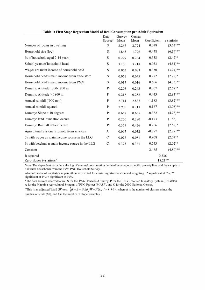
The first stage model of consumption, which is estimated over 830 rural households from the

sample survey, is reported in Table 1. The particular specification of the model resulted from

a detailed model discovery process, with many sensitivity checks.6 Briefly, the modelling

6 Details are available in an unpublished working paper from the authors.

8

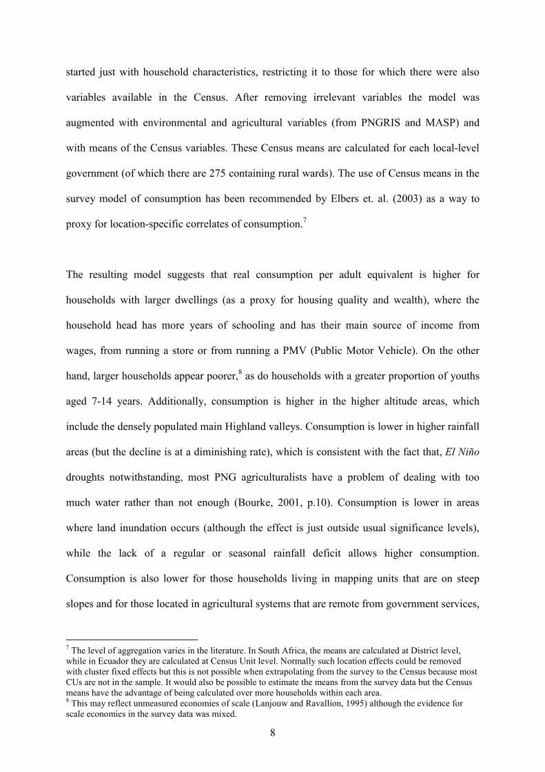
started just with household characteristics, restricting it to those for which there were also

variables available in the Census. After removing irrelevant variables the model was

augmented with environmental and agricultural variables (from PNGRIS and MASP) and

with means of the Census variables. These Census means are calculated for each local-level

government (of which there are 275 containing rural wards). The use of Census means in the

survey model of consumption has been recommended by Elbers et. al. (2003) as a way to

proxy for location-specific correlates of consumption.7

The resulting model suggests that real consumption per adult equivalent is higher for

households with larger dwellings (as a proxy for housing quality and wealth), where the

household head has more years of schooling and has their main source of income from

wages, from running a store or from running a PMV (Public Motor Vehicle). On the other

hand, larger households appear poorer,8 as do households with a greater proportion of youths

aged 7-14 years. Additionally, consumption is higher in the higher altitude areas, which

include the densely populated main Highland valleys. Consumption is lower in higher rainfall

areas (but the decline is at a diminishing rate), which is consistent with the fact that, El Niño

droughts notwithstanding, most PNG agriculturalists have a problem of dealing with too

much water rather than not enough (Bourke, 2001, p.10). Consumption is lower in areas

where land inundation occurs (although the effect is just outside usual significance levels),

while the lack of a regular or seasonal rainfall deficit allows higher consumption.

Consumption is also lower for those households living in mapping units that are on steep

slopes and for those located in agricultural systems that are remote from government services,

7 The level of aggregation varies in the literature. In South Africa, the means are calculated at District level, while in Ecuador they are calculated at Census Unit level. Normally such location effects could be removed with cluster fixed effects but this is not possible when extrapolating from the survey to the Census because most CUs are not in the sample. It would also be possible to estimate the means from the survey data but the Census means have the advantage of being calculated over more households within each area. 8 This may reflect unmeasured economies of scale (Lanjouw and Ravallion, 1995) although the evidence for scale economies in the survey data was mixed.

9

where remoteness is measured as being more than eight hours travel from a minor centre.

Consumption is also higher, the greater is the proportion of the households in the LLG whose

heads draw their main income from wages, and the greater the proportion engaged in betel

nut production and trade.

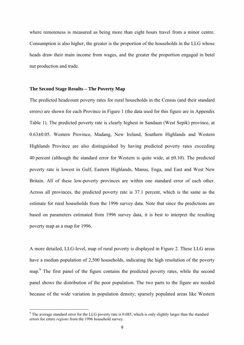
The Second Stage Results – The Poverty Map

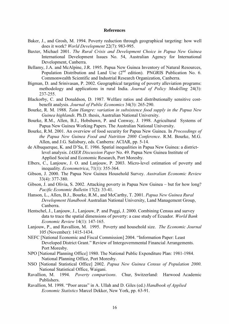
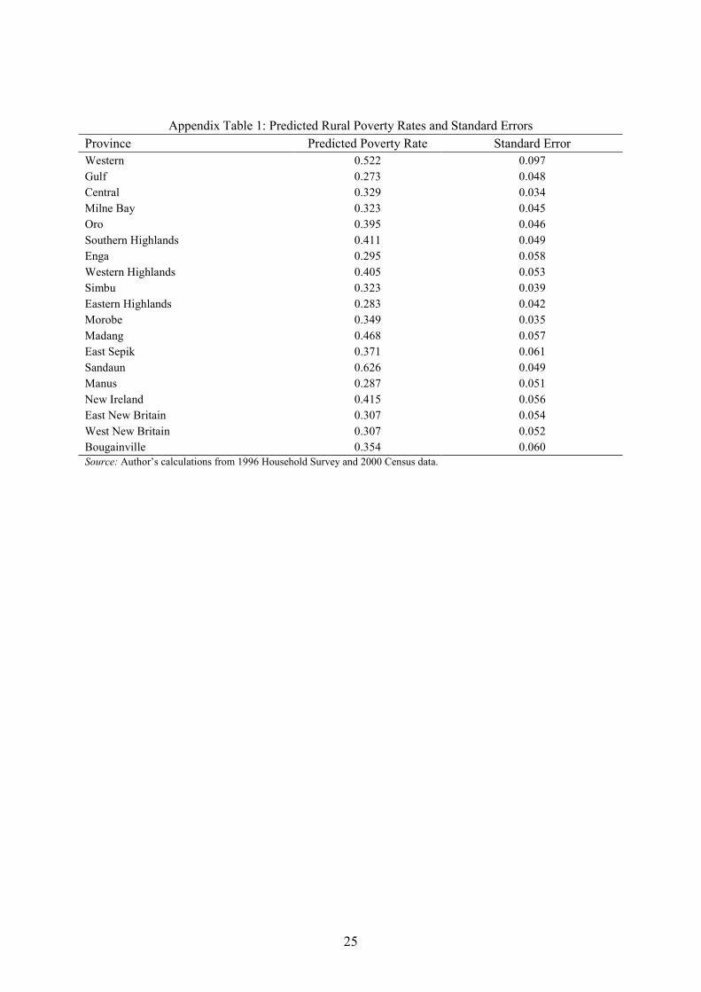
The predicted headcount poverty rates for rural households in the Census (and their standard

errors) are shown for each Province in Figure 1 (the data used for this figure are in Appendix

Table 1). The predicted poverty rate is clearly highest in Sandaun (West Sepik) province, at

0.63±0.05. Western Province, Madang, New Ireland, Southern Highlands and Western

Highlands Province are also distinguished by having predicted poverty rates exceeding

40 percent (although the standard error for Western is quite wide, at ±0.10). The predicted

poverty rate is lowest in Gulf, Eastern Highlands, Manus, Enga, and East and West New

Britain. All of these low-poverty provinces are within one standard error of each other.

Across all provinces, the predicted poverty rate is 37.1 percent, which is the same as the

estimate for rural households from the 1996 survey data. Note that since the predictions are

based on parameters estimated from 1996 survey data, it is best to interpret the resulting

poverty map as a map for 1996.

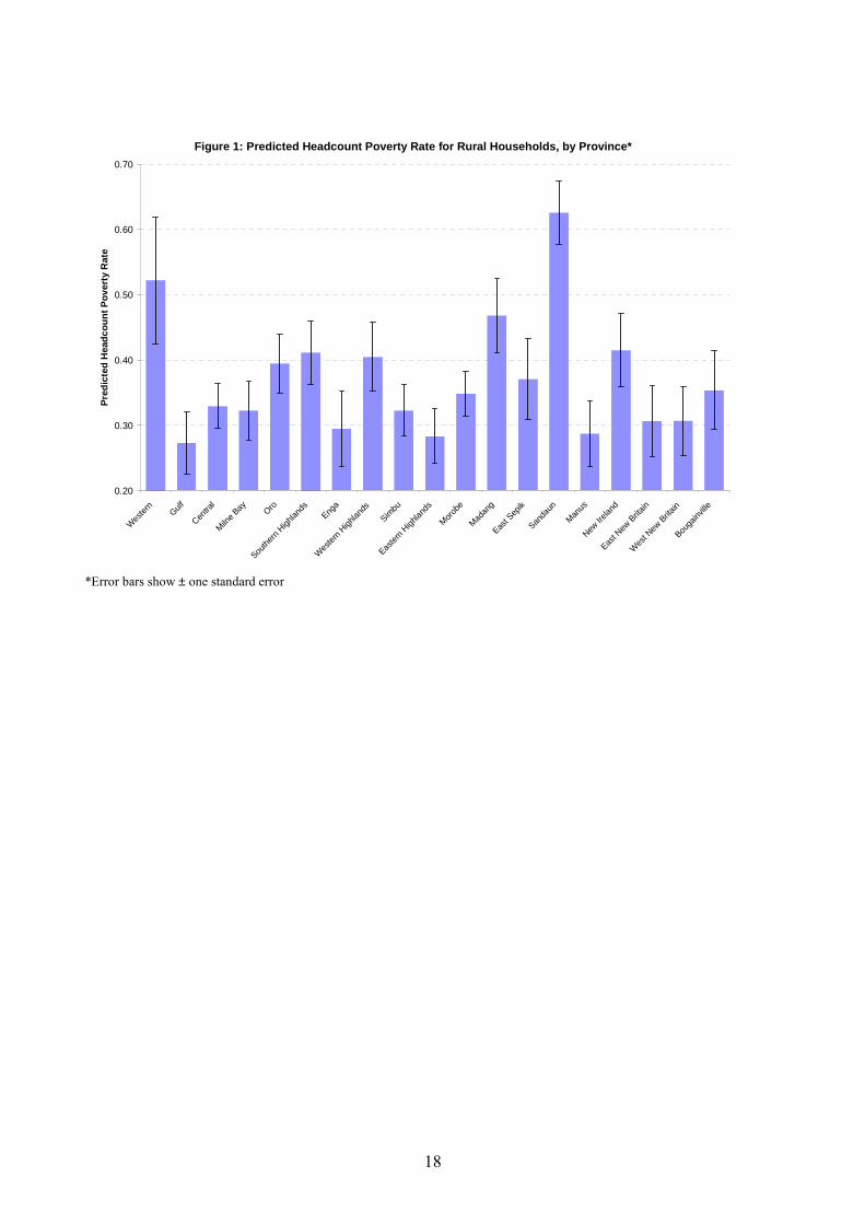
A more detailed, LLG-level, map of rural poverty is displayed in Figure 2. These LLG areas

have a median population of 2,500 households, indicating the high resolution of the poverty

map.9 The first panel of the figure contains the predicted poverty rates, while the second

panel shows the distribution of the poor population. The two parts to the figure are needed

because of the wide variation in population density; sparsely populated areas like Western

9 The average standard error for the LLG poverty rate is 0.085, which is only slightly larger than the standard errors for entire regions from the 1996 household survey.

10

Province appear more important than they actually are if attention is focused only on the

poverty rates. On the other hand, even though some areas of the Highlands have low poverty

rates, the greatest number of poor people is found in that region.

A general description of the pattern in Figure 2 is that the lowest rural poverty rates are found

in areas surrounding Port Moresby and Lae, along much of the Highlands Highway, in

coastal areas where Oil Palm is significant, and in areas adjacent to major mining projects

like Ok Tedi. The highest poverty rates are in the provinces bordering Irian Jaya (except the

area around Ok Tedi), along the fringe areas beside the central Highland valleys and

extending along the mountainous center to the tip of the island of New Guinea, and in

localised areas of the New Guinea islands (especially parts of Pomio and Natamanai). The

greatest density of poverty is found in Western Highlands, Southern Highlands and East

Sepik Provinces.

Although provincial boundaries are not highlighted in Figure 2, it is clear that many

provinces have LLGs from both the highest poverty class and the lowest poverty class. This

heterogeneity would be missed if high resolution poverty maps are not used. Thus, simply

concentrating on provincial-level averages of poverty statistics (or other welfare indicators)

may prove to be a misleading guide for any targeted interventions.

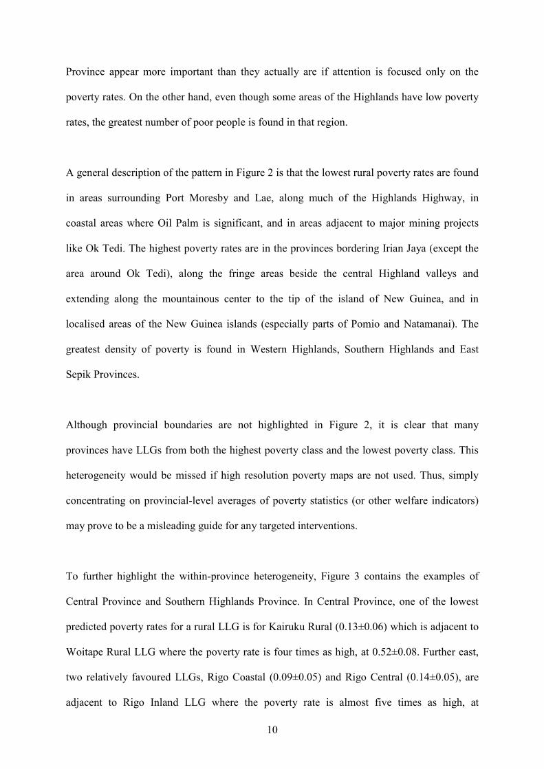
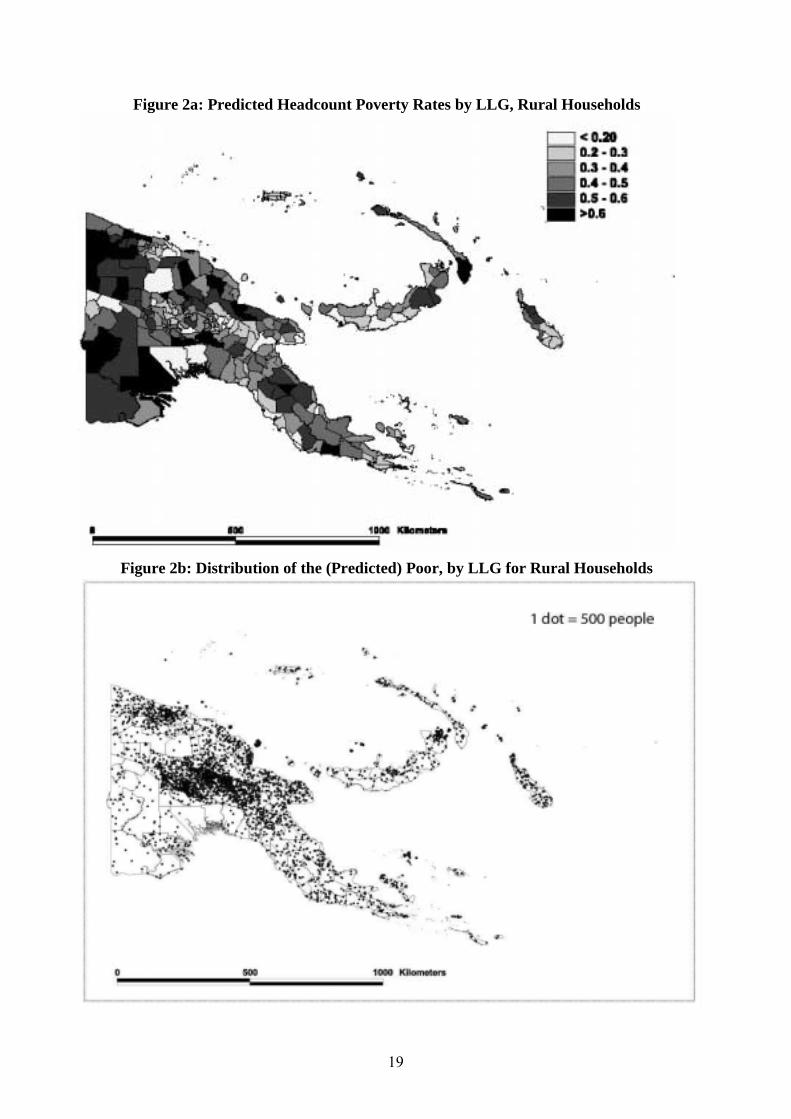
To further highlight the within-province heterogeneity, Figure 3 contains the examples of

Central Province and Southern Highlands Province. In Central Province, one of the lowest

predicted poverty rates for a rural LLG is for Kairuku Rural (0.13±0.06) which is adjacent to

Woitape Rural LLG where the poverty rate is four times as high, at 0.52±0.08. Further east,

two relatively favoured LLGs, Rigo Coastal (0.09±0.05) and Rigo Central (0.14±0.05), are

adjacent to Rigo Inland LLG where the poverty rate is almost five times as high, at

11

0.60±0.06. In the Southern Highlands, poverty rates are very high in LLGs around the

northwest and southeast borders of the province (Erave (0.62 ± 0.11), Awi-Pori (0.59±0.12),

Lake Kopiago (0.57 ± 0.06) and Hulia (0.59 ± 0.12)). But in contrast, the northeast border

(the closest to Mt Hagen) has some LLGs with quite low poverty rates, including Ialibu Basin

(0.22 ± 0.06) and East Pangia (0.17 ± 0.07). These areas with low poverty rates are adjacent

to other LLGs where the poverty rates are approximately 50 percent.

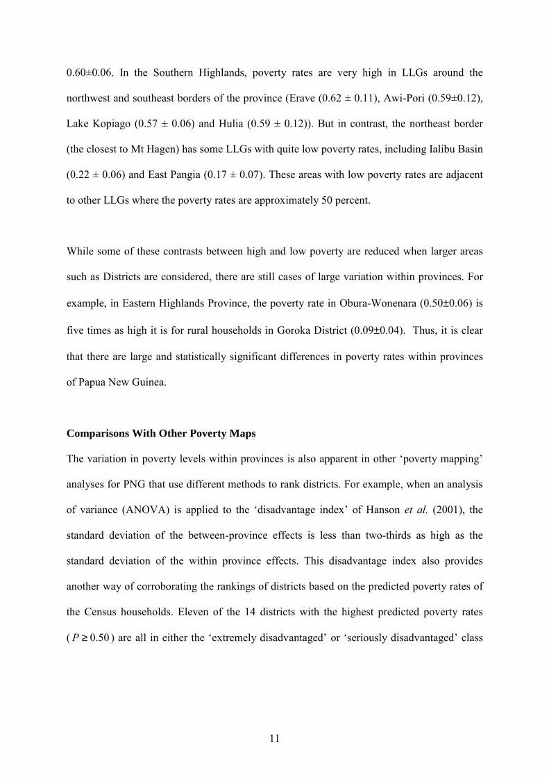
While some of these contrasts between high and low poverty are reduced when larger areas

such as Districts are considered, there are still cases of large variation within provinces. For

example, in Eastern Highlands Province, the poverty rate in Obura-Wonenara (0.50±0.06) is

five times as high it is for rural households in Goroka District (0.09±0.04). Thus, it is clear

that there are large and statistically significant differences in poverty rates within provinces

of Papua New Guinea.

Comparisons With Other Poverty Maps

The variation in poverty levels within provinces is also apparent in other �poverty mapping�

analyses for PNG that use different methods to rank districts. For example, when an analysis

of variance (ANOVA) is applied to the �disadvantage index� of Hanson et al. (2001), the

standard deviation of the between-province effects is less than two-thirds as high as the

standard deviation of the within province effects. This disadvantage index also provides

another way of corroborating the rankings of districts based on the predicted poverty rates of

the Census households. Eleven of the 14 districts with the highest predicted poverty rates

( 50.0≥P ) are all in either the �extremely disadvantaged� or �seriously disadvantaged� class

12

of Hanson et al. (2001).10 The correlation between the predicted poverty rate and the

disadvantage index is 0.28, which is highly significant, as is the rank correlation of 0.26.

There is an even closer fit with the District Development Index of the NEFC, where the

correlation with the predicted poverty rates is 0.64. However, this is less informative because

the predicted poverty rates were one component used in the calculation of the District

Development Index, so the close relationship is not surprising.

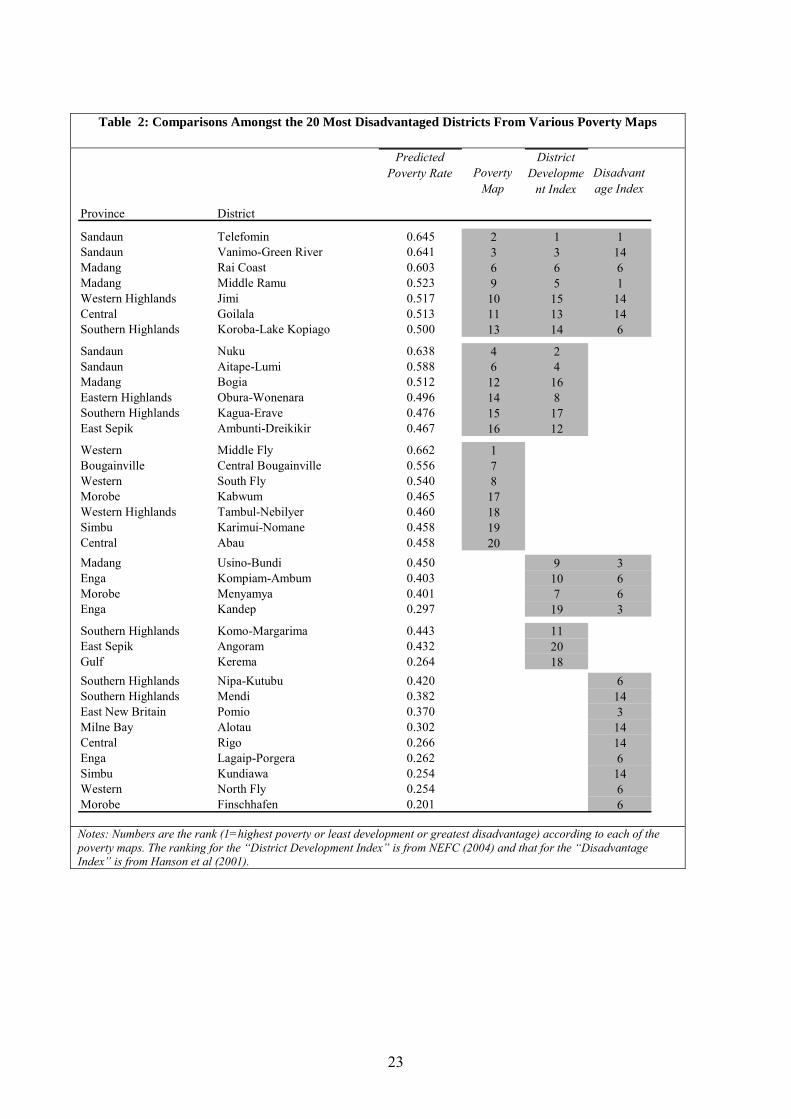
A comparison of the District rankings from the current poverty map with the rankings made

by Hanson et al. (2001) and the NEFC is presented in Table 2. The 20 most disadvantaged

Districts identified from each of the three studies are listed, and the degree of overlap is

highlighted. There are seven Districts that are identified by all three studies as being amongst

the 20 worst (Telefomin, Vanimo-Green River, Rai Coast, Middle Ramu, Jimi, Goilala, and

Koroba-Lake Kopiago). Another six Districts are identified by the current poverty map and

the NEFC study. Clearly, while there is some variation in the individual studies, the overall

agreement suggests that it should be possible to identify an agreed upon set of poor areas. In

many cases these same areas were identified up to 30 years ago (Wilson, 1974).

Implications for Targeting

The poverty maps indicate considerable variation in poverty rates within some provinces.

This variation means that public spending interventions that try to target �poor� provinces are

likely to miss large numbers of people in poor areas in other provinces, while also benefiting

people in non-poor areas in the designated provinces. To formalise the impression presented

by the maps, a decomposition of inequality into within- and between-area components was

carried out. If most inequality is due to within-area sources, targeting poor areas is still likely

10 Nine of these 14 (Telefomin, Middle Ramu, Goilala, Vanimo-Green River, Aitape-Lumi, Koroba-Kopiago, Jimi, Oburu-Wonenara, and Rai Coast) are also listed amongst the most disadvantaged districts in the studies of Wilson (1974).

13

to see a lot of leakage to non-poor households, while the untargeted areas are also likely to

include many poor households, leading to problems of undercoverage. Of course, the

contribution of the between- and within-area components of inequality will vary with the

choice of targeting level. At finer levels of disaggregation, more of the total inequality will be

due to between-area sources.

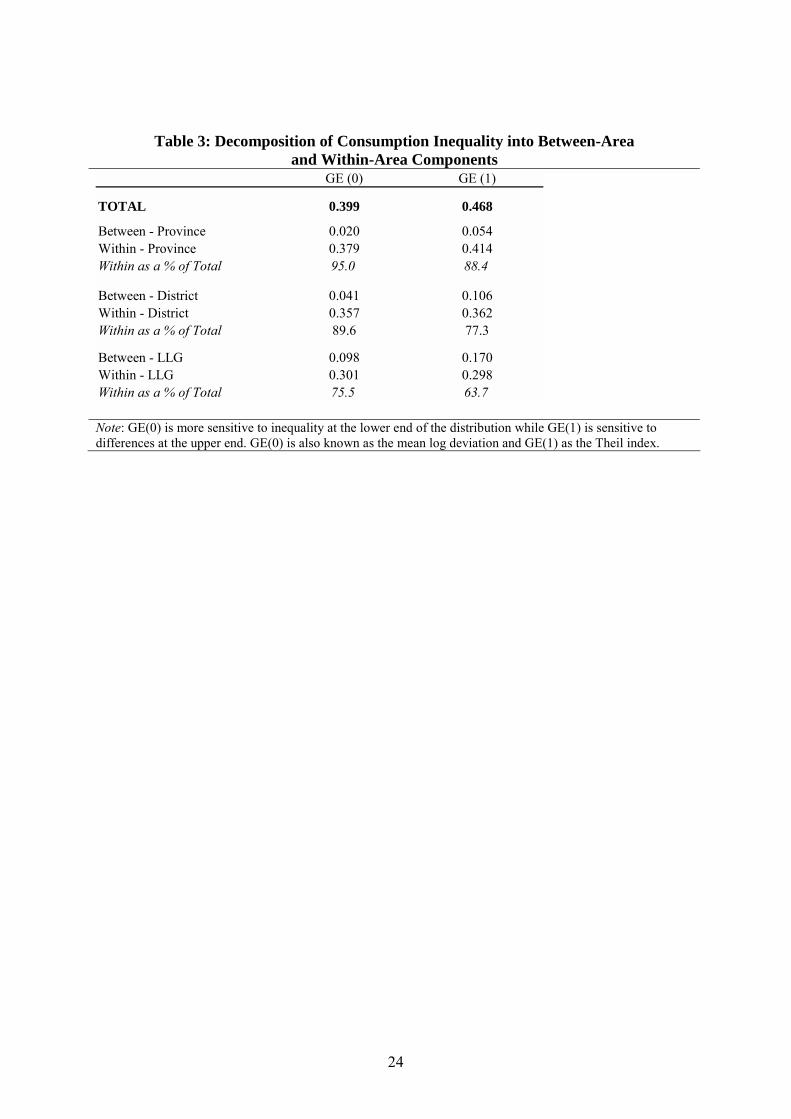
According to the generalized entropy class of inequality measures, between 88 and 95 percent

of consumption inequality in PNG is due to within- rather than between-province sources

(Table 3).11 The relative unimportance of between-province variation suggests that any

geographical targeting might be most effective for smaller, sub-provincial areas. But even at

the District level, more than three-quarters of inequality is within-District rather than between

Districts. Indeed, even at the LLG level, only one-quarter to one-third of total inequality in

predicted real consumption per adult equivalent is due to between-area inequality. This high

degree of within-area inequality will be a major impediment to any area-based programs that

hope to target only poor people.

In light of the significant variation in poverty rates between areas in the same provinces, it

would be most useful to have information on current transfers to LLGs and Districts. These

flows could then be compared with their predicted poverty rates. In terms of poverty

reduction, inter-governmental transfers should act to compensate for higher levels of poverty,

in the sense that poorer sub-national areas get larger per head transfers. The current system

within PNG, whereby District Support Grants are allocated as a lump sum irrespective of

population or level of need, is unlikely to obey this pattern. Most other grants from the

national government are made to the provinces, while the allocation within provinces is left

11 GE(0) is more sensitive to inequality at the lower end of the distribution while GE(1) is sensitive to differences at the upper end. GE(0) is also known as the mean log deviation and GE(1) as the Theil index.

14

to be determined by the provincial governments. However, information on grants at the sub-

provincial level is not currently available.

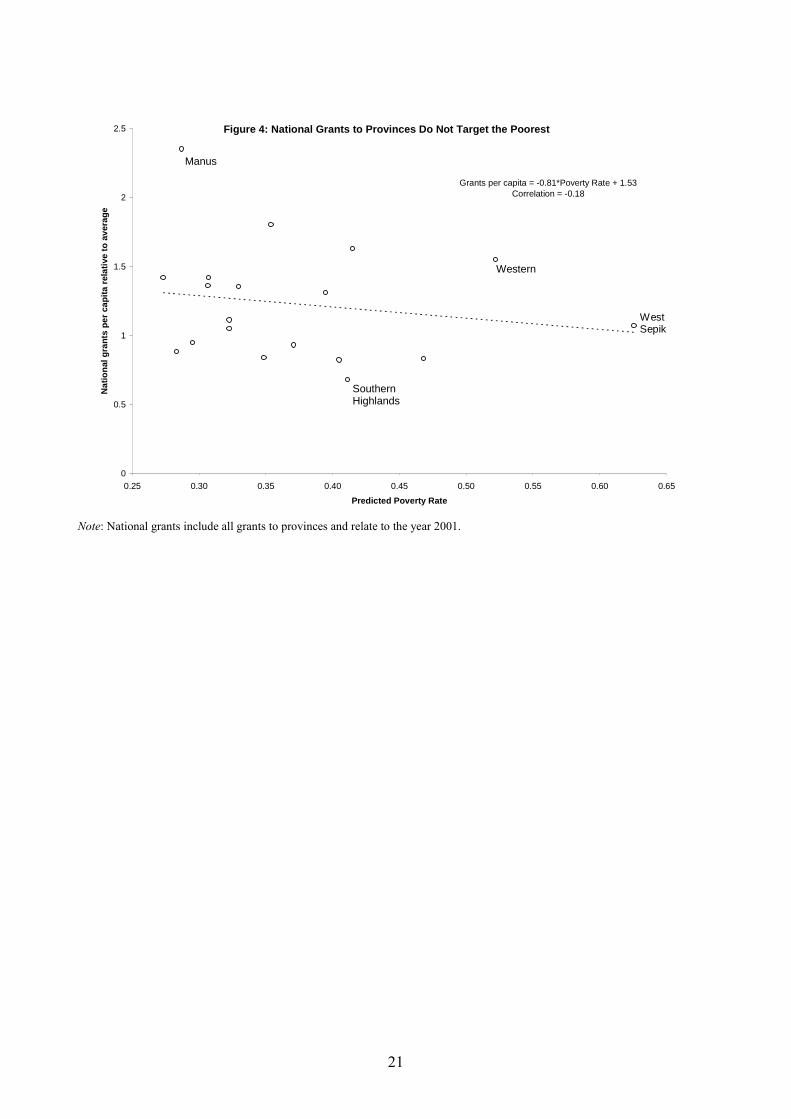
In the absence of District-level and LLG-level information, we have been able to obtain

information on a variety of transfers made to Provinces. It appears that per capita national

grants are negatively correlated with the predicted poverty rate in each Province (Figure 4).

In other words, it appears that poorer Provinces receive smaller transfers. Thus, current

transfers between government levels in PNG do not appear to be favourable to poor areas.

Given the high degree of within-Province variability, any redesign of these transfers should

consider targeting poorer Districts or LLGs within Provinces, although even then it would be

a relatively blunt targeting instrument unless combined with other household-level targeting

mechanisms.

Conclusions

In this paper, disaggregated maps of poverty in rural Papua New Guinea have been created by

using recently developed �poverty mapping� techniques. These techniques rely on regression

modelling to combine information from the 1996 Household Survey with data from the 2000

Census and from resource and agricultural mapping databases with national coverage.

Predicted poverty head-count rates have been presented at provincial, district and LLG levels.

These same three administrative levels have been used to decompose inequality in predicted

consumption into within-area and between-area components.

A common theme in all of the results is that there is a high level of within-province

heterogeneity. A policy implication of this heterogeneity is that public spending interventions

that try to target poor provinces are likely to miss large numbers of poor people in other

provinces, while also benefiting the non-poor in the areas selected for interventions. To better

15

reach the poor, a combination of sub-provincial and household-level targeting would

probably be needed. Another theme is the persistence of poverty in some areas. Almost 30

years ago, many of the same areas were identified as disadvantaged. This inability to bring

the fruits of development to these areas shows the considerable challenge posed by poverty

reduction in Papua New Guinea.

16

References

Baker, J., and Grosh, M. 1994. Poverty reduction through geographical targeting: how well does it work? World Development 22(7): 983-995.

Baxter, Michael 2001. The Rural Crisis and Development Choice in Papua New Guinea International Development Issues No. 54, Australian Agency for International Development, Canberra.

Bellamy, J.A. and McAlpine, J.R. 1995. Papua New Guinea Inventory of Natural Resources, Population Distribution and Land Use (2nd edition). PNGRIS Publication No. 6. Commonwealth Scientific and Industrial Research Organization, Canberra.

Bigman, D. and Srinivasan, P. 2002. Geographical targeting of poverty alleviation programs: methodology and applications in rural India. Journal of Policy Modelling 24(3): 237-255.

Blackorby, C. and Donaldson, D. 1987. Welfare ratios and distributionally sensitive cost-benefit analysis. Journal of Public Economics 34(3): 265-290.

Bourke, R. M. 1988. Taim Hangre: variation in subsistence food supply in the Papua New Guinea highlands. Ph.D. thesis, Australian National University.

Bourke, R.M., Allen, B.J., Hobsbawn, P. and Conway, J. 1998. Agricultural Systems of Papua New Guinea Working Papers. The Australian National University.

Bourke, R.M. 2001. An overview of food security for Papua New Guinea. In Proceedings of the Papua New Guinea Food and Nutrition 2000 Conference. R.M. Bourke, M.G. Allen, and J.G. Salisbury, eds. Canberra: ACIAR, pp. 5-14.

de Albuquerque, K. and D�Sa, E. 1986. Spatial inequalities in Papua New Guinea: a district-level analysis. IASER Discussion Paper No. 49. Papua New Guinea Institute of Applied Social and Economic Research, Port Moresby.

Elbers, C., Lanjouw, J. O. and Lanjouw, P. 2003. Micro-level estimation of poverty and inequality. Econometrica, 71(1): 355-364.

Gibson, J. 2000. The Papua New Guinea Household Survey. Australian Economic Review 33(4): 377-380.

Gibson, J. and Olivia, S. 2002. Attacking poverty in Papua New Guinea � but for how long? Pacific Economic Bulletin 17(2): 33-41.

Hanson, L., Allen, B.J., Bourke, R.M., and McCarthy, T. 2001. Papua New Guinea Rural Development Handbook Australian National University, Land Management Group, Canberra.

Hentschel, J., Lanjouw, J., Lanjouw, P. and Poggi, J. 2000. Combining Census and survey data to trace the spatial dimensions of poverty: a case study of Ecuador. World Bank Economic Review 14(1): 147-165.

Lanjouw, P., and Ravallion, M. 1995. Poverty and household size. The Economic Journal 105 (November): 1415-1434.

NEFC [National Economic and Fiscal Commission] 2004. �Information Paper: Least Developed District Grant.� Review of Intergovernmental Financial Arrangements. Port Moresby.

NPO [National Planning Office] 1980. The National Public Expenditure Plan: 1981-1984. National Planning Office, Port Moresby.

NSO [National Statistical Office] 2002. Papua New Guinea Census of Population 2000. National Statistical Office, Waigani.

Ravallion, M. 1994. Poverty comparisons. Chur, Switzerland: Harwood Academic Publishers.

Ravallion, M. 1998. �Poor areas� in A. Ullah and D. Giles (ed.) Handbook of Applied Economic Statistics Marcel Dekker, New York, pp. 63-91.

17

Wilson, R. 1974. Socio-economic indicators applied to sub-districts of Papua New Guinea. Economic Geography Department Discussion Paper 1. Melbourne University, Melbourne.

World Bank. 1999. Papua New Guinea: Poverty and Access to Public Services. World Bank: Washington, DC.

18

Figure 1: Predicted Headcount Poverty Rate for Rural Households, by Province*

0.20

0.30

0.40

0.50

0.60

0.70

Wes

tern

Gulf

Centra

l

Milne B

ay Oro

Southe

rn High

lands

Enga

Wes

tern H

ighlan

dsSim

bu

Easter

n High

lands

Morobe

Madan

g

East S

epik

Sanda

un

Manus

New Ire

land

East N

ew B

ritain

Wes

t New

Brita

in

Bouga

inville

Pred

icte

d H

eadc

ount

Pov

erty

Rat

e

*Error bars show ± one standard error

19

Figure 2a: Predicted Headcount Poverty Rates by LLG, Rural Households

Figure 2b: Distribution of the (Predicted) Poor, by LLG for Rural Households

20

Figure 3: Predicted Headcount Poverty Rates and Standard Errors for LLGs in Central and Southern Highlands Provinces

21

Figure 4: National Grants to Provinces Do Not Target the Poorest

Grants per capita = -0.81*Poverty Rate + 1.53Correlation = -0.18

0

0.5

1

1.5

2

2.5

0.25 0.30 0.35 0.40 0.45 0.50 0.55 0.60 0.65

Predicted Poverty Rate

Nat

iona

l gra

nts

per c

apita

rela

tive

to a

vera

ge

Note: National grants include all grants to provinces and relate to the year 2001.

Manus

West Sepik

Southern Highlands

Western

22

Table 1: First Stage Regression Model of Real Consumption per Adult Equivalent

Data Sourcea

Survey Mean

Census Mean

Coefficient

t-statistic

Number of rooms in dwelling S 3.267 2.774 0.078 (3.63)**

Household size (log) S 1.865 1.796 -0.478 (6.39)**

% of household aged 7-14 years S 0.229 0.204 -0.358 (2.42)*

School years of household head S 3.186 3.218 0.033 (4.51)**

Wages are main income of household head S 0.062 0.083 0.350 (3.24)**

Household head�s main income from trade store S 0.061 0.045 0.272 (2.22)*

Household head�s main income from PMV S 0.017 0.016 0.656 (4.33)**

Dummy: Altitude 1200-1800 m P 0.298 0.263 0.307 (2.57)*

Dummy: Altitude > 1800 m P 0.218 0.258 0.443 (2.83)**

Annual rainfall (�000 mm) P 2.714 2.837 -1.183 (3.82)**

Annual rainfall squared P 7.900 8.713 0.167 (3.08)**

Dummy: Slope > 10 degrees P 0.657 0.635 -0.382 (4.28)**

Dummy: land inundation occurs P 0.250 0.280 -0.173 (1.63)

Dummy: Rainfall deficit is rare P 0.357 0.426 0.266 (2.62)*

Agricultural System is remote from services A 0.067 0.032 -0.377 (2.87)**

% with wages as main income source in the LLG C 0.077 0.081 0.908 (2.07)*

% with betelnut as main income source in the LLG C 0.375 0.361 0.553 (2.02)*

Constant 2.465 (4.80)**

R-squared 0.336 Zero-slopes F-statisticb 18.21** Note: The dependent variable is the log of nominal consumption deflated by a region-specific poverty line, and the sample is 830 rural households from the 1996 PNG Household Survey. Absolute value of t-statistics in parentheses corrected for clustering, stratification and weighting. * significant at 5%; ** significant at 1%; + significant at 10%. a The data sources referred to are: S for the 1996 Household Survey, P for the PNG Resource Inventory System (PNGRIS), A for the Mapping Agricultural Systems of PNG Project (MASP), and C for the 2000 National Census. b This is an adjusted Wald (W) test: ( ) )1,(~1 +−+− kdkFWkdkd , where d is the number of clusters minus the number of strata (60), and k is the number of slope variables.

23

Table 2: Comparisons Amongst the 20 Most Disadvantaged Districts From Various Poverty Maps

Notes: Numbers are the rank (1=highest poverty or least development or greatest disadvantage) according to each of the poverty maps. The ranking for the �District Development Index� is from NEFC (2004) and that for the �Disadvantage Index� is from Hanson et al (2001).

Poverty Map

Disadvantage Index

Province District

Sandaun Telefomin 0.645 2 1 1Sandaun Vanimo-Green River 0.641 3 3 14Madang Rai Coast 0.603 6 6 6Madang Middle Ramu 0.523 9 5 1Western Highlands Jimi 0.517 10 15 14Central Goilala 0.513 11 13 14Southern Highlands Koroba-Lake Kopiago 0.500 13 14 6

Sandaun Nuku 0.638 4 2Sandaun Aitape-Lumi 0.588 6 4Madang Bogia 0.512 12 16Eastern Highlands Obura-Wonenara 0.496 14 8Southern Highlands Kagua-Erave 0.476 15 17East Sepik Ambunti-Dreikikir 0.467 16 12

Western Middle Fly 0.662 1Bougainville Central Bougainville 0.556 7Western South Fly 0.540 8Morobe Kabwum 0.465 17Western Highlands Tambul-Nebilyer 0.460 18Simbu Karimui-Nomane 0.458 19Central Abau 0.458 20Madang Usino-Bundi 0.450 9 3Enga Kompiam-Ambum 0.403 10 6Morobe Menyamya 0.401 7 6Enga Kandep 0.297 19 3

Southern Highlands Komo-Margarima 0.443 11East Sepik Angoram 0.432 20Gulf Kerema 0.264 18Southern Highlands Nipa-Kutubu 0.420 6Southern Highlands Mendi 0.382 14East New Britain Pomio 0.370 3Milne Bay Alotau 0.302 14Central Rigo 0.266 14Enga Lagaip-Porgera 0.262 6Simbu Kundiawa 0.254 14Western North Fly 0.254 6Morobe Finschhafen 0.201 6

Predicted Poverty Rate

District Developme

nt Index

24

Table 3: Decomposition of Consumption Inequality into Between-Area and Within-Area Components

Note: GE(0) is more sensitive to inequality at the lower end of the distribution while GE(1) is sensitive to differences at the upper end. GE(0) is also known as the mean log deviation and GE(1) as the Theil index.

GE (0) GE (1)

TOTAL 0.399 0.468

Between - Province 0.020 0.054Within - Province 0.379 0.414Within as a % of Total 95.0 88.4

Between - District 0.041 0.106Within - District 0.357 0.362Within as a % of Total 89.6 77.3

Between - LLG 0.098 0.170Within - LLG 0.301 0.298Within as a % of Total 75.5 63.7

25

Appendix Table 1: Predicted Rural Poverty Rates and Standard Errors Province Predicted Poverty Rate Standard Error Western 0.522 0.097 Gulf 0.273 0.048 Central 0.329 0.034 Milne Bay 0.323 0.045 Oro 0.395 0.046 Southern Highlands 0.411 0.049 Enga 0.295 0.058 Western Highlands 0.405 0.053 Simbu 0.323 0.039 Eastern Highlands 0.283 0.042 Morobe 0.349 0.035 Madang 0.468 0.057 East Sepik 0.371 0.061 Sandaun 0.626 0.049 Manus 0.287 0.051 New Ireland 0.415 0.056 East New Britain 0.307 0.054 West New Britain 0.307 0.052 Bougainville 0.354 0.060 Source: Author�s calculations from 1996 Household Survey and 2000 Census data.