manifold regularization - mit.edu9.520/spring09/classes/class08_manifold.pdf · riemannian...

Manifold Regularization

Lorenzo Rosasco

9.520 Class 08

March 2, 2008

L. Rosasco Manifold Regularization

About this class

Goal To analyze the limits of learning from examples inhigh dimensional spaces. To introduce thesemi-supervised setting and the use of unlabeleddata to learn the intrinsic geometry of a problem.To define Riemannian Manifolds, ManifoldLaplacians, Graph Laplacians. To introduce a newclass of algorithms based on ManifoldRegularization (LapRLS, LapSVM).


Unlabeled data

Why using unlabeled data?

labeling is often an “expensive” processsemi-supervised learning is the natural setting for humanlearning


Semi-supervised Setting

u i.i.d. samples drawn on X from the marginal distribution p(x)

{x1, x2, . . . , xu},

only n of which endowed with labels drawn from the conditionaldistributions p(y |x)

{y1, y2, . . . , yn}.

The extra u − n unlabeled samples give additional informationabout the marginal distribution p(x).


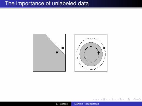
The importance of unlabeled data


Curse of dimensionality and p(x)

Assume X is the D-dimensional hypercube [0,1]D. The worstcase scenario corresponds to uniform marginal distributionp(x).

Local MethodsA prototype example of the effect of high dimentionality can beseen in nearest methods techniques. As d increases, localtechniques (eg nearest neighbors) become rapidly ineffective.


Curse of dimensionality and k-NN

It would seem that with a reasonably large set of trainingdata, we could always approximate the conditionalexpectation by k-nearest-neighbor averaging.We should be able to find a fairly large set of observationsclose to any x ∈ [0,1]D and average them.This approach and our intuition break down in highdimensions.


Sparse sampling in high dimension

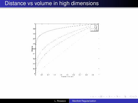
Suppose we send out a cubical neighborhood about one vertexto capture a fraction r of the observations. Since thiscorresponds to a fraction r of the unit volume, the expectededge length will be

eD(r) = r1D .

Already in ten dimensions e10(0.01) = 0.63, that is to capture1% of the data, we must cover 63% of the range of each inputvariable!No more ”local” neighborhoods!


Distance vs volume in high dimensions


Intrinsic dimensionality

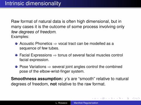
Raw format of natural data is often high dimensional, but inmany cases it is the outcome of some process involving onlyfew degrees of freedom.Examples:

Acoustic Phonetics⇒ vocal tract can be modelled as asequence of few tubes.

Facial Expressions⇒ tonus of several facial muscles controlfacial expression.

Pose Variations⇒ several joint angles control the combinedpose of the elbow-wrist-finger system.

Smoothness assumption: y ’s are “smooth” relative to naturaldegrees of freedom, not relative to the raw format.


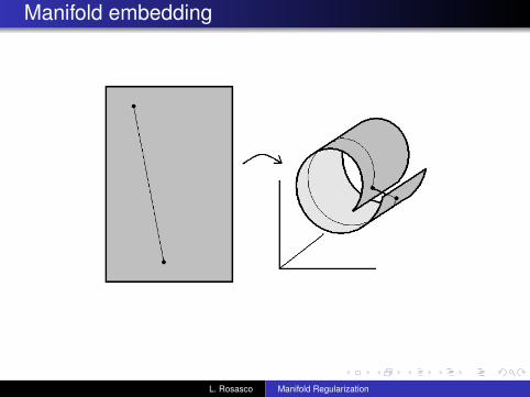
Manifold embedding


Riemannian Manifolds

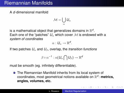
A d-dimensional manifold

M =⋃α

Uα

is a mathematical object that generalizes domains in Rd .Each one of the “patches” Uα which coverM is endowed with asystem of coordinates

α : Uα → Rd .

If two patches Uα and Uβ , overlap, the transition functions

β ◦ α−1 : α(Uα⋂

Uβ)→ Rd

must be smooth (eg. infinitely differentiable).

The Riemannian Manifold inherits from its local system ofcoordinates, most geometrical notions available on Rd : metrics,angles, volumes, etc.


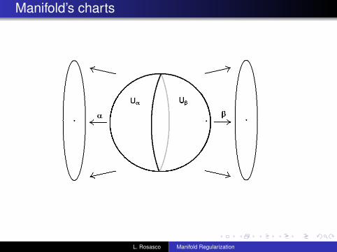
Manifold’s charts


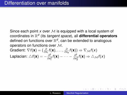
Differentiation over manifolds

Since each point x overM is equipped with a local system ofcoordinates in Rd (its tangent space), all differential operatorsdefined on functions over Rd , can be extended to analogousoperators on functions overM.Gradient: ∇f (x) = ( ∂

∂x1f (x), . . . , ∂

∂xdf (x))⇒ ∇Mf (x)

Laplacian: 4f (x) = − ∂2

∂x21f (x)− · · · − ∂2

∂x2df (x)⇒4Mf (x)


Measuring smoothness overM

Given f :M→ R

∇Mf (x) represents amplitude and direction of variationaround xS(f ) =

∫M ‖∇Mf (x)‖2dp(x) is a global measure of

smoothness for fStokes’ theorem (generalization of integration by parts)links gradient and Laplacian

S(f ) =

∫M‖∇Mf (x)‖2dp(x) =

∫M

f (x)4Mf (x)dp(x)


Manifold regularization Belkin, Niyogi,Sindhwani, 04

A new class of techniques which extend standard Tikhonovregularization over RKHS, introducing the additional regularizer‖f‖2

I =∫M f (x)4Mf (x)dp(x) to enforce smoothness of solutions

relative to the underlying manifold

f ∗ = arg minf∈H

1n

n∑i=1

V (f (xi ), yi ) + λA‖f‖2K + λI

∫M

f (x)4Mf (x)dp(x)

λI controls the complexity of the solution in the intrinsicgeometry ofM.

λA controls the complexity of the solution in the ambient space.


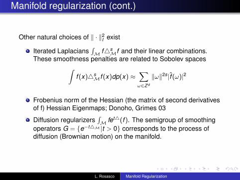
Manifold regularization (cont.)

Other natural choices of ‖ · ‖2I exist

Iterated Laplacians∫M f4s

Mf and their linear combinations.These smoothness penalties are related to Sobolev spaces∫

f (x)4sMf (x)dp(x) ≈

∑ω∈Z d

‖ω‖2s |̂f (ω)|2

Frobenius norm of the Hessian (the matrix of second derivativesof f) Hessian Eigenmaps; Donoho, Grimes 03

Diffusion regularizers∫M fet4(f ). The semigroup of smoothing

operators G = {e−t4M |t > 0} corresponds to the process ofdiffusion (Brownian motion) on the manifold.


An empirical proxy of the manifold

We cannot compute the intrinsic smoothness penalty

‖f‖2I =

∫M

f (x)4Mf (x)dp(x)

because we don’t know the manifoldM and the embedding

Φ :M→ RD.

But we assume that the unlabeled samples are drawn i.i.d.from the uniform probability distribution overM and thenmapped into RD by Φ


Neighborhood graph

Our proxy of the manifold is a weighted neighborhood graphG = (V ,E ,W ), with vertices V given by the points{x1, x2, . . . , xu}, edges E defined by one of the two followingadjacency rules

connect xi to its k nearest neighborhoodsconnect xi to ε-close points

and weights Wij associated to two connected vertices

Wij = e−‖xi−xj‖

2

ε

Note: computational complexity O(u2)


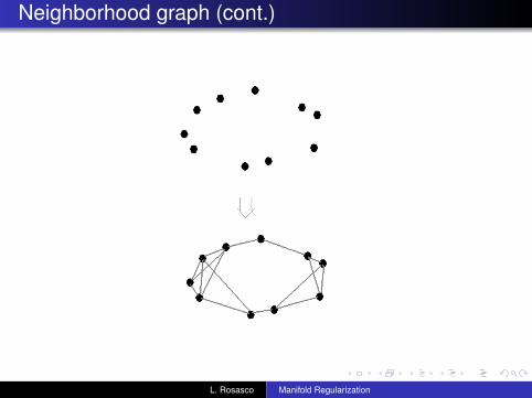
Neighborhood graph (cont.)


The graph Laplacian

The graph Laplacian over the weighted neighborhood graph(G,E ,W ) is the matrix

Lij = Dii −Wij , Dii =∑

j

Wij .

L is the discrete counterpart of the manifold Laplacian 4M

fT Lf =n∑

i,j=1

Wij(fi − fj)2 ≈

∫M‖∇f (x)‖2dp(x).

Analogous properties of the eigensystem: nonnegativespectrum, null spaceLooking for rigorous convergence results


A convergence theorem Belkin, Niyogi, 05

Operator L: “out-of-sample extension” of the graph Laplacian L

L(f )(x) =∑

i

(f (x)− f (xi))e−‖x−xi‖

2

ε x ∈ X , f : X → R

Theorem: Let the u data points {x1, . . . , xu} be sampled fromthe uniform distribution over the embedded d-dimensionalmanifoldM. Put ε = u−α, with 0 < α < 1

2+d . Then for allf ∈ C∞ and x ∈ X , there is a constant C, s.t. in probability,

limu→∞

Cε−

d+22

uL(f )(x) = 4Mf (x).


Laplacian-based regularization algorithms (Belkin et al. 04)

Replacing the unknown manifold Laplacian with the graphLaplacian ‖f‖2I = 1

u2 fT Lf, where f is the vector [f (x1), . . . , f (xu)],we get the minimization problem

f ∗ = arg minf∈H

1n

n∑i=1

V (f (xi), yi) + λA‖f‖2K +λI

u2 fT Lf

λI = 0: standard regularization (RLS and SVM)λA → 0: out-of-sample extension for Graph Regularizationn = 0: unsupervised learning, Spectral Clustering


The Representer Theorem

Using the same type of reasoning used in Class 3, aRepresenter Theorem can be easily proved for the solutions ofManifold Regularization algorithms.The expansion range over all the supervised andunsupervised data points

f (x) =u∑

j=1

cjK (x , xj).


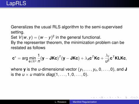
LapRLS

Generalizes the usual RLS algorithm to the semi-supervisedsetting.Set V (w , y) = (w − y)2 in the general functional.By the representer theorem, the minimization problem can berestated as follows

c∗ = arg minc∈Ru

1n

(y− JKc)T (y− JKc) + λAcT Kc +λI

u2 cT KLKc,

where y is the u-dimensional vector (y1, . . . , yn,0, . . . ,0), and Jis the u × u matrix diag(1, . . . ,1,0, . . . ,0).


LapRLS (cont.)

The functional is differentiable, strictly convex and coercive.The derivative of the object function vanishes at the minimizerc∗

1n

KJ(y− JKc∗) + (λAK +λInu2 KLK)c∗ = 0.

From the relation above and noticing that due to the positivity ofλA, the matrix M defined below, is invertible, we get

c∗ = M−1y,

where

M = JK + λAnI +λIn2

u2 LK.


LapSVM

Generalizes the usual SVM algorithm to the semi-supervisedsetting.Set V (w , y) = (1− yw)+ in the general functional above.Applying the representer theorem, introducing slack variablesand adding the unpenalized bias term b, we easily get theprimal problem

c∗ = arg minc∈Ru ,ξ∈Rn

1n∑n

i=1 ξi + λAcT Kc + λIu2 cT KLKc

subject to : yi(∑u

j=1 cjK (xi , xj) + b) ≥ 1− ξi i = 1, . . . ,nξi ≥ 0 i = 1, . . . ,n


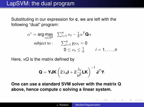
LapSVM: the dual program

Substituting in our expression for c, we are left with thefollowing “dual” program:

α∗ = arg maxα∈Rn

∑ni=1 αi − 1

2αT Qα

subject to :∑n

i=1 yiαi = 00 ≤ αi ≤ 1

n i = 1, . . . ,n

Here, vQ is the matrix defined by

Q = YJK(

2λAI + 2λI

u2 LK)−1

JT Y.

One can use a standard SVM solver with the matrix Qabove, hence compute c solving a linear system.


Numerical experimentshttp://manifold.cs.uchicago.edu/manifold_regularization

Two Moons DatasetHandwritten Digit RecognitionSpoken Letter Recognition


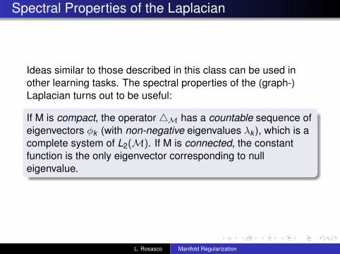
Spectral Properties of the Laplacian

Ideas similar to those described in this class can be used inother learning tasks. The spectral properties of the (graph-)Laplacian turns out to be useful:

If M is compact, the operator 4M has a countable sequence ofeigenvectors φk (with non-negative eigenvalues λk ), which is acomplete system of L2(M). If M is connected, the constantfunction is the only eigenvector corresponding to nulleigenvalue.


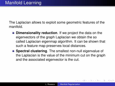
Manifold Learning

The Laplacian allows to exploit some geometric features of themanifold.

Dimensionality reduction. If we project the data on theeigenvectors of the graph Laplacian we obtain the socalled Laplacian eigenmap algorithm. It can be shown thatsuch a feature map preserves local distances.Spectral clustering. The smallest non-null eigenvalue ofthe Laplacian is the value of the minimum cut on the graphand the associated eigenvector is the cut.


manifold regularization - mit.edu9.520/spring09/classes/class08_manifold.pdf · riemannian...

Documents