making sense of the subprime crisis - brookings · creditworthiness of subprime borrowers, so many...
TRANSCRIPT
69
SHANE M. SHERLUNDBoard of Governors of the
Federal Reserve System
PAUL WILLENFederal Reserve Bank of Boston
Making Sense of the Subprime Crisis
ABSTRACT Should market participants have anticipated the large increasein home foreclosures in 2007 and 2008? Most of these foreclosures stemmedfrom mortgage loans originated in 2005 and 2006, raising suspicions thatlenders originated many extremely risky loans during this period. We showthat although these loans did carry extra risk factors, particularly increasedleverage, reduced underwriting standards alone cannot explain the dramaticrise in foreclosures. We also investigate whether market participants under-estimated the likelihood of a fall in home prices or the sensitivity of fore-closures to falling prices. We show that given available data, they shouldhave understood that a significant price drop would raise foreclosures sharply,although loan-level (as opposed to ownership-level) models would have pre-dicted a smaller rise than occurred. Analyst reports and other contemporarydiscussions reveal that analysts generally understood that falling prices wouldhave disastrous consequences but assigned that outcome a low probability.
Had market participants anticipated the increase in defaults on sub-prime mortgages originated in 2005 and 2006, the nature and extent
of the current financial market disruptions would be very different. Exante, investors in subprime mortgage-backed securities (MBSs) wouldhave demanded higher returns and greater capital cushions. As a result,borrowers would not have found credit as cheap or as easy to obtain as itbecame during the subprime credit boom of those years. Rating agencieswould have reacted similarly, rating a much smaller fraction of each dealinvestment grade. As a result, the subsequent increase in foreclosureswould have been significantly smaller, with fewer attendant disruptionsin the housing market, and investors would not have suffered such out-sized, and unexpected, losses. To make sense of the subprime crisis, oneneeds to understand why, when accepting significant exposure to the
KRISTOPHER GERARDIFederal Reserve Bank of Atlanta
ANDREAS LEHNERTBoard of Governors of the
Federal Reserve System
11472-02_Gerardi_rev3.qxd 3/6/09 12:24 PM Page 69

creditworthiness of subprime borrowers, so many smart analysts, armedwith advanced degrees, data on the past performance of subprime borrow-ers, and state-of-the-art modeling technology, did not anticipate that somany of the loans they were buying, either directly or indirectly, wouldgo bad.
Our bottom line is that the problem largely had to do with expecta-tions about home prices. Had investors known the future trajectory ofhome prices, they would have predicted large increases in delinquency anddefault and losses on subprime MBSs roughly consistent with what hasoccurred. We show this by using two different methods to travel back to2005, when the subprime market was still thriving, and look forward fromthere. The first method is to forecast performance using only data availablein 2005, and the second is to look at what market participants wrote at thetime. The latter, “narrative” analysis provides strong evidence againstthe claim that investors lost money because they purchased loans that,because they were originated by others, could not be evaluated properly.
Our first order of business, however, is to address the more basic ques-tion of whether the subprime mortgages that defaulted were themselvesunreasonable ex ante—an explanation commonly offered for the crisis.We show that the problem loans, most of which were originated in 2005and 2006, were not that different from loans made earlier, which hadperformed well despite carrying a variety of serious risk factors. Thatsaid, we document that loans in the 2005–06 cohort were riskier, and wedescribe in detail the dimensions along which risk increased. In particu-lar, we find that borrower leverage increased and, further, did so in a waythat was relatively opaque to investors. However, we also find that thechange in the mix of mortgages originated is too slight to explain the hugeincrease in defaults. Put simply, the average default rate on loans origi-nated in 2006 exceeds the default rate on the riskiest category of loansoriginated in 2004.
We then turn to the role of the collapse in home price appreciation(HPA) that started in the spring of 2006.1 To have invested large sums insubprime mortgages in 2005 and 2006, lenders must have expected eitherthat HPA would remain high (or at least not collapse) or that subprimedefaults would be insensitive to a big drop in HPA. More formally, letting
70 Brookings Papers on Economic Activity, Fall 2008
1. The relationship between foreclosures and HPA in the subprime crisis is well docu-mented. See Gerardi, Shapiro, and Willen (2007), Mayer, Pence, and Sherlund (forthcom-ing), Demyanyk and van Hemert (2007), Doms, Furlong, and Krainer (2007), and Danis andPennington-Cross (2005).
11472-02_Gerardi_rev3.qxd 3/6/09 12:24 PM Page 70

f represent foreclosures, p prices, and t time, we can decompose the growthin foreclosures over time, df/dt, into a part corresponding to the sensitivityof foreclosures to price changes and a part reflecting the change in pricesover time:
Our goal is to determine whether market participants underestimateddf/dp, the sensitivity of foreclosures to price changes, or whether dp/dt, thetrajectory of home prices, came out much worse than they expected.
Our first time-travel exercise, as mentioned, uses data that were avail-able to investors ex ante on mortgage performance, to determine whether itwas possible at the time to estimate df/dp on subprime mortgages accurately.Because severe home price declines are relatively rare and the subprimemarket is relatively new, one plausible theory is that the data lacked sufficient variation to allow df/dp to be estimated in scenarios in which dp/dtis negative and large. We put ourselves in the place of analysts in 2005,using data through 2004 to estimate the type of hazard models commonlyused in the industry to predict mortgage defaults. We use two datasets. Thefirst is a loan-level dataset from First American LoanPerfomance that isused extensively in the industry to track the performance of mortgagespackaged in MBSs; it has sparse information on loans originated before1999. The second is a dataset from the Warren Group, which has trackedthe fates of homebuyers in Massachusetts since the late 1980s. These dataare not loan-level but rather ownership-level data; that is, the unit of observation is a homeowner’s tenure in a property, which may encompassmore than one mortgage loan. The Warren Group data were not (so far aswe can tell) widely used by the industry but were, at least in theory, avail-able and, unlike the loan-level data, do contain information on the behav-ior of homeowners in an environment of falling prices.
We find that it was possible, although not necessarily easy, to measuredf/dp with some degree of accuracy. Essentially, a researcher with perfectforesight about the trajectory of prices from 2005 forward would haveforecast a large increase in foreclosures starting in 2007. Perhaps themost interesting result is that despite the absence of negative HPA in1998–2004, when almost all subprime loans were originated, we could stilldetermine, albeit not exactly, the likely behavior of subprime borrowers inan environment of falling home prices. In effect, the out-of-sample (andout-of-support) performance of default models was sufficiently good tohave predicted large losses in such an environment.
d d d d d df t f p p t= × .
GERARDI, LEHNERT, SHERLUND, and WILLEN 71
11472-02_Gerardi_rev3.qxd 3/6/09 12:24 PM Page 71

Although it was thus possible to estimate df/dp, we also find that therelationship was less exact when using the data on loans rather than thedata on ownerships. A given borrower might refinance his or her originalloan several times before defaulting. Each of these successive loans exceptthe final one would have been seen by lenders as successful. An owner-ship, in contrast, terminates only when the homeowner sells and moves, oris foreclosed upon and evicted. Thus, although the same foreclosure wouldappear as a default in both loan-level and ownership-level data, the inter-mediate refinancings between purchase and foreclosure—the “happyendings”—would not appear in an ownership-level database.
Our second time-travel exercise explores what analysts of the mort-gage market said in 2004, 2005, and 2006 about the loans that eventuallygot into trouble. Our conclusion is that investment analysts had a goodsense of df/dp and understood, with remarkable accuracy, how fallingdp/dt would affect the performance of subprime mortgages and thesecurities backed by them. As an illustrative example, consider a 2005analyst report published by a large investment bank:2 analyzing arepresentative deal composed of 2005 vintage loans, the report argued itwould face 17 percent cumulative losses in a “meltdown” scenario inwhich house prices fell 5 percent over the life of the deal. That analysiswas prescient: the ABX index, a widely used price index of asset-backedsecurities, currently implies that such a deal will actually face losses of18.3 percent over its life. The problem was that the report assigned onlya 5 percent probability to the meltdown scenario, where home prices fell5 percent, whereas it assigned probabilities of 15 percent and 50 percent toscenarios in which home prices rose 11 percent and 5 percent, respectively,over the life of the deal.
We argue that the fall in home prices outweighs other changes in driving up foreclosures in the recent period. However, we do not take aposition on why prices rose so rapidly, why they fell so fast, or why theypeaked in mid-2006. Other researchers have examined whether factorssuch as lending standards can affect home prices.3 Broadly speaking, wemaintain the assumption that although, in the aggregate, lending standardsmay indeed have affected home price dynamics (we are agnostic on this
72 Brookings Papers on Economic Activity, Fall 2008
2. This is the bank designated Bank B in our discussion of analyst reports below, in areport dated August 15, 2005.
3. Examples include Pavlov and Wachter (2006), Coleman, LaCour-Little, and Vandell(2008), Wheaton and Lee (2008), Wheaton and Nechayev (2008), and Sanders and others(2008).
11472-02_Gerardi_rev3.qxd 3/6/09 12:24 PM Page 72

point), no individual market participant felt that his or her actions couldaffect prices. Nor do we analyze whether housing was overvalued in 2005and 2006, such that a fall in prices was to some extent predictable. Therewas a lively debate during that period, with some arguing that housing wasreasonably valued and others that it was overvalued.4
Our results suggest that some borrowers were more sensitive to a singlemacro risk factor, namely, home prices. This comports well with the find-ings of David Musto and Nicholas Souleles, who argue that averagedefault rates are only half the story: correlations across borrowers, perhapsdriven by macroeconomic forces, are also an important factor in valuingportfolios of consumer loans.5
In this paper we focus almost exclusively on subprime mortgages.However, many of the same arguments might also apply to prime mort-gages. Deborah Lucas and Robert McDonald compute the price volatil-ity of the assets underlying securities issued by the housing-relatedgovernment-sponsored enterprises (GSEs).6 Concentrating mainly onprime and near-prime mortgages and using information on the firms’leverage and their stock prices, these authors find that risk was quite high(and, as a result, that the value of the implicit government guarantee onGSE debt was quite high).
Many have argued that a major driver of the subprime crisis was theincreased use of securitization.7 In this view, the “originate to distribute”business model of many mortgage finance companies separated the under-writer making the credit extension decision from exposure to the ultimatecredit quality of the borrower, and thus created an incentive to maximizelending volume without concern for default rates. At the same time, infor-mation asymmetries, unfamiliarity with the market, or other factors pre-vented investors, who were accepting the credit risk, from putting in placeeffective controls on these incentives. Although this argument is intu-itively persuasive, our results are not consistent with such an explanation.One of our key findings is that most of the uncertainty about lossesstemmed from uncertainty about the future direction of home prices, notfrom uncertainty about the quality of the underwriting. All that said, our
GERARDI, LEHNERT, SHERLUND, and WILLEN 73
4. Among the first group were Himmelberg, Mayer, and Sinai (2005) and McCarthy andPeach (2004); the pessimists included Gallin (2006, 2008) and Davis, Lehnert, and Martin(2008).
5. Musto and Souleles (2006).6. Lucas and McDonald (2006).7. See, for example, Keys and others (2008) and Calomiris (2008).
11472-02_Gerardi_rev3.qxd 3/6/09 12:24 PM Page 73

models do not perfectly predict the defaults that occurred, and they oftenunderestimate the number of defaults. One possible explanation is thatthere was an unobservable deterioration of underwriting standards in 2005and 2006.8 But another is that our model of the highly nonlinear relation-ship between prices and foreclosures is wanting. No existing research hassuccessfully distinguished between these two explanations.
The endogeneity of prices does present a problem for our estimation.One common theory is that foreclosures drive price declines by increasingthe supply of homes for sale, in effect introducing a new term into thedecomposition of df/dt, namely, dp/df. However, our estimation techniquesare to a large extent robust to this issue. As discussed by Gerardi, AdamShapiro, and Willen,9 most of the variation in the key explanatory vari-able, homeowner’s equity, is within-town (or, more precisely, within-metropolitan-statistical-area), within-quarter variation and thus could notbe driven by differences in foreclosures over time or across towns. In fact,as we will show, one can estimate the effect of home prices on foreclosureseven in periods when there were very few foreclosures, and in periods inwhich foreclosed properties sold quickly.
No discussion of the subprime crisis is complete without mention of theinterest rate resets built into many subprime mortgages, which virtuallyguaranteed large increases in monthly payments. Many commentatorshave attributed the crisis to the payment shock associated with the firstreset of subprime 2/28 adjustable-rate mortgages (these are 30-year ARMswith 2-year teaser rates). However, the evidence from loan-level datashows that resets cannot account for a significant portion of the increase inforeclosures. Christopher Mayer, Karen Pence, and Sherlund, as well asChristopher Foote and coauthors, show that the overwhelming majority ofdefaults on subprime ARMs occur long before the first reset.10 In effect,many lenders would have been lucky had borrowers waited until the firstreset to default.
The rest of the paper is organized as follows. We begin in the next sec-tion by documenting changes in underwriting standards on mortgages. Thefollowing section explores what researchers could have learned with thedata they had in 2005. In the penultimate section we review contemporaryanalyst reports. The final section presents some conclusions.
74 Brookings Papers on Economic Activity, Fall 2008
8. This explanation is favored by Demyanyk and van Hemert (2007).9. Gerardi, Shapiro, and Willen (2007).10. Mayer, Pence, and Sherlund (forthcoming); Foote and others (2008a).
11472-02_Gerardi_rev3.qxd 3/6/09 12:24 PM Page 74

Underwriting Standards in the Subprime Market
We begin with a brief background on subprime mortgages, including adiscussion of the competing definitions of “subprime.” We then discusschanges in the apparent credit risk of subprime mortgages originated from1999 to 2007, and we link those changes to the actual performance of thoseloans. We argue that the increased number of subprime loans that wereoriginated with high loan-to-value (LTV) ratios was the most importantobservable risk factor that increased over the period. Further, we arguethat the increases in leverage were to some extent masked from investorsin MBSs. Loans originated with less than complete documentation ofincome or assets, and particularly loans originated with both high lever-age and incomplete documentation, exhibited sharper subsequent rises indefault rates than other loans. A more formal decomposition exercise,however, confirms that the rise in defaults can only partly be explained byobserved changes in underwriting standards.
Some Background on Subprime Mortgages
One of the first notable features encountered by researchers working onsubprime mortgages is the dense thicket of jargon surrounding the field,particularly the multiple competing definitions of “subprime.” This ham-pers attempts to estimate the importance of subprime lending. There are,effectively, four useful ways to categorize a loan as subprime. First, mort-gage servicers themselves recognize that certain borrowers require morefrequent contact in order to ensure timely payment, and they charge higherfees to service these loans; thus, one definition of a subprime loan is onethat is classified as subprime by the servicer. Second, some lenders spe-cialize in loans to financially troubled borrowers, and the Department ofHousing and Urban Development maintains a list of such lenders; loansoriginated by these “HUD list” lenders are often taken as a proxy for sub-prime loans. Third, “high-cost” loans are defined as loans that carry feesand interest rates significantly above those charged to typical borrowers.Fourth, a subprime loan is sometimes defined as any loan packaged into anMBS that is marketed as containing subprime loans.
Table 1 reports two measures of the importance of subprime lending inthe United States. The first is the percent of loans in the Mortgage BankersAssociation (MBA) delinquency survey that are classified as “subprime.”Because the MBA surveys mortgage servicers, this measure is based onthe first definition above. As the table shows, over the past few years,subprime mortgages by this definition have accounted for about 12 to
GERARDI, LEHNERT, SHERLUND, and WILLEN 75
11472-02_Gerardi_rev3.qxd 3/6/09 12:24 PM Page 75
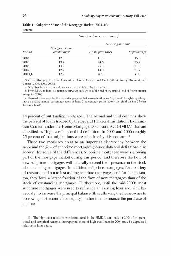
14 percent of outstanding mortgages. The second and third columns showthe percent of loans tracked by the Federal Financial Institutions Examina-tion Council under the Home Mortgage Disclosure Act (HMDA) that areclassified as “high cost”—the third definition. In 2005 and 2006 roughly25 percent of loan originations were subprime by this measure.11
These two measures point to an important discrepancy between thestock and the flow of subprime mortgages (source data and definitions alsoaccount for some of the difference). Subprime mortgages were a growingpart of the mortgage market during this period, and therefore the flow ofnew subprime mortgages will naturally exceed their presence in the stockof outstanding mortgages. In addition, subprime mortgages, for a varietyof reasons, tend not to last as long as prime mortgages, and for this reason,too, they form a larger fraction of the flow of new mortgages than of thestock of outstanding mortgages. Furthermore, until the mid-2000s mostsubprime mortgages were used to refinance an existing loan and, simulta-neously, to increase the principal balance (thus allowing the homeowner toborrow against accumulated equity), rather than to finance the purchase ofa home.
76 Brookings Papers on Economic Activity, Fall 2008
11. The high-cost measure was introduced in the HMDA data only in 2004; for opera-tional and technical reasons, the reported share of high-cost loans in 2004 may be depressedrelative to later years.
Table 1. Subprime Share of the Mortgage Market, 2004–08a
Percent
Subprime loans as a share of
Mortgage loansNew originationsc
Period outstandingb Home purchases Refinancings
2004 12.3 11.5 15.52005 13.4 24.6 25.72006 13.7 25.3 31.02007 12.7 14.0 21.72008Q2 12.2 n.a. n.a.
Sources: Mortgage Bankers Association; Avery, Canner, and Cook (2005); Avery, Brevoort, andCanner (2006, 2007, 2008).
a. Only first liens are counted; shares are not weighted by loan value.b. From MBA national delinquency surveys; data are as of the end of the period (end of fourth quarter
except for 2008).c. Share of loans used for the indicated purpose that were classified as “high cost” (roughly speaking,
those carrying annual percentage rates at least 3 percentage points above the yield on the 30-yearTreasury bond).
11472-02_Gerardi_rev3.qxd 3/6/09 12:24 PM Page 76
In this section we will focus on changes in the kinds of loans made overthe period 1999–2007. We will use loan-level data on mortgages sold intoprivate-label MBSs marketed as subprime. These data (known as theTrueStandings Securities ABS data) are provided by First AmericanLoanPerformance and were widely used in the financial services industrybefore and during the subprime boom. We further limit the set of loansanalyzed to the three most popular products: those carrying fixed interestrates to maturity and the so-called 2/28s and 3/27s. As alluded to above, a2/28 is a 30-year mortgage in which the contract rate is fixed at an initial,teaser rate for two years; after that it adjusts to the six-month LIBOR (London interbank offer rate) plus a predetermined margin (often around 6percentage points). A 3/27 is defined analogously. Together these three loancategories account for more than 98 percent of loans in the original data.
In this section the outcome variable of interest is whether a mortgagedefaults within 12 months of its first payment due date. There are severalcompeting definitions of “default”; here we define a mortgage as havingdefaulted by month 12 if, as of its 12th month of life, it had terminated fol-lowing a foreclosure notice, or if the loan was listed as real estate ownedby the servicer (indicating a transfer of title from the borrower), or if theloan was still active but foreclosure proceedings had been initiated, or ifpayments on the loan were 90 or more days past due. Note that some of theloans we count as defaults might subsequently have reverted to “current”status, if the borrower made up missed payments. In effect, any borrowerwho manages to make 10 of the first 12 mortgage payments, or who re-finances or sells without a formal notice of default having been filed, isassumed to have not defaulted.
Figure 1 tracks the default rate in the ABS data under this definitionfrom 1999 through 2006. Conceptually, default rates differ from delin-quency rates in that they track the fate of mortgages originated in a givenmonth by their 12th month of life; in effect, the default rate tracks theproportion of mortgages originated at a given point that are “dead” bymonth 12. Delinquency rates, by contrast, track the proportion of all activemortgages that are “sick” at a given point in calendar time. Further,because we close our dataset in December 2007, we can track the fate ofonly those mortgages originated through December 2006. The continuedsteep increase in mortgage distress is not reflected in these data, nor is thefate of mortgages originated in 2007, although we do track the underwrit-ing characteristics of these mortgages.
Note that this measure of default is designed to allow one to comparethe ex ante credit risk of various underwriting terms. It is of limited
GERARDI, LEHNERT, SHERLUND, and WILLEN 77
11472-02_Gerardi_rev3.qxd 3/6/09 12:24 PM Page 77

usefulness as a predictor of defaults, because it considers only what hap-pens by the 12th month of a mortgage, and it does not consider changesin the home prices, interest rates, or the overall economic environmentfaced by households. Further, this measure does not consider the changingincentives to refinance. The competing-risks duration models we estimatein a later section are, for these reasons, far better suited to determining thecredit and prepayment outlook for a group of mortgages.
Changes in Underwriting Standards
During the credit boom, lenders published daily “rate sheets” showing,for various combinations of loan risk characteristics, the interest rates theywould charge to make such loans. A simple rate sheet, for example, mightbe a matrix of credit scores and LTV ratios; borrowers with lower creditscores or higher LTV ratios would be charged higher interest rates or berequired to pay larger fees up front. Loans for certain cells of the matrixrepresenting combinations of low credit scores and high LTV ratios mightnot be available at all.
Unfortunately, we do not have access to information on changes in ratesheets over time, but underwriting standards can change in ways that are
78 Brookings Papers on Economic Activity, Fall 2008
Sources: First American LoanPerformance; authors’ calculations.a. Share of all subprime mortgages originated in the indicated month that default within 12 months of
origination.
5
10
20
Percent
2002 2006
Origination date
25
15
2000 2004
Figure 1. Twelve-Month Default Rate on Subprime Mortgagesa
11472-02_Gerardi_rev3.qxd 3/6/09 12:24 PM Page 78

observable in the ABS data. Of course, underwriting standards can alsochange in ways observable to the loan originator but not reflected in theABS data, or in ways largely unobservable even by the loan originator (forexample, an increase in borrowers getting home equity lines of credit afterorigination). In this section we consider the evidence that more loans withex ante observable risky characteristics were originated during the boom.Throughout we use loans from the ABS database described earlier.
We consider trends over time in borrower credit scores, loan documen-tation, leverage, and other factors associated with risk, such as the purposeof the loan, non-owner-occupancy, and amortization schedules. We findthat from 1999 to 2007, borrower leverage, loans with incomplete docu-mentation, loans used to purchase homes (as opposed to refinancing an existing loan), and loans with nontraditional amortization schedules all grew. Borrower credit scores increased, while loans to non-owner-occupants remained essentially flat. Of these variables, the increase in bor-rower leverage appears to have contributed the most to the increase indefaults, and we find some evidence that leverage was, in the ABS data atleast, opaque.
CREDIT SCORES. Credit scores, which essentially summarize a bor-rower’s history of missing debt payments, are the most obvious indicatorof prime or subprime status. The most commonly used scalar credit scoreis the FICO score originally developed by Fair, Isaac & Co. It is the onlyscore contained in the ABS data, although subprime lenders often usedscores and other information from all three credit reporting bureaus.
Under widely accepted industry rules of thumb, borrowers with FICOscores of 680 or above are not usually considered subprime without someother accompanying risk factor, borrowers with credit scores between 620and 680 may be considered subprime, and those with credit scores below620 are rarely eligible for prime loans. Subprime pricing models typicallyused more information than just a borrower’s credit score; they also con-sidered the nature of the missed payment that led a borrower to have a lowcredit score. For example, a pricing system might weight missed mortgagepayments more than missed credit card payments.
Figure 2 shows the proportions of newly originated subprime loansfalling into each of these three categories. The proportion of such loansto borrowers with FICO scores of 680 and above grew over the sampleperiod, while loans to traditionally subprime borrowers (those with scoresbelow 620) accounted for a smaller share of originations.
LOAN DOCUMENTATION. Borrowers (or their mortgage brokers) submita file with each mortgage application documenting the borrower’s income,
GERARDI, LEHNERT, SHERLUND, and WILLEN 79
11472-02_Gerardi_rev3.qxd 3/6/09 12:24 PM Page 79

liquid assets, and other debts, and the value of the property being used ascollateral. Media attention has focused on the rise of so-called low-doc orno-doc loans, for which documentation of income or assets was incom-plete. (These include the infamous “stated-income” loans.) The top leftpanel of figure 3 shows that the proportion of newly originated subprimeloans carrying less than full documentation rose from around 20 percentin 1999 to a high of more than 35 percent by mid-2006. Thus, althoughreduced-documentation lending was a part of subprime lending, it was byno means the majority of the business, nor did it increase dramatically dur-ing the credit boom.
As we discuss in greater detail below, until about 2004, subprime loanswere generally backed by substantial equity in the property. This was espe-cially true for subprime loans with less than complete documentation.Thus, in some sense the lender accepted less complete documentation inexchange for a greater security interest in the underlying property.
LEVERAGE. The leverage of a property is, in principle, the total value ofall liens on the property divided by its value. This is often referred to asthe property’s combined loan-to-value, or CLTV, ratio. Both the numera-tor and the denominator of the CLTV ratio will fluctuate over a borrower’stenure in the property: the borrower may amortize the original loan, refi-
80 Brookings Papers on Economic Activity, Fall 2008
Sources: First American LoanPerformance; authors’ calculations.
20
40
80
Percent
2000 2004
Origination date
60
2002 2006
FICO ≥ 680
620 ≤ FICO < 680
FICO < 620
Figure 2. Distribution of Subprime Mortgages by FICO Score at Origination
11472-02_Gerardi_rev3.qxd 3/6/09 12:24 PM Page 80

nance, or take on junior liens, and the potential sale price of the home willchange over time. However, the current values of all of these variablesought to be known at the time of a loan’s origination. The lender under-takes a title search to check for the presence of other liens and hires anappraiser to confirm either the price paid (when the loan is used to pur-chase a home) or the potential sale price of the property (when the loan isused to refinance an existing loan).
In practice, high leverage during the boom was also accompanied byadditional complications and opacity. Rather than originate a single loanfor the desired amount, originators often preferred to originate two loans:one for 80 percent of the property’s value, and the other for the remainingdesired loan balance. In the event of a default, the holder of the first lienwould be paid first from the sale proceeds, with the junior lien holder
GERARDI, LEHNERT, SHERLUND, and WILLEN 81
Sources: First American LoanPerformance; authors’ calculations.a. CLTV ratio ≥ 90 percent or including a junior lien.
Percent
2004
Origination date
2002 2006
Low documentation
10
20
30
40
50
2000
Percent
2004
Origination date
2002 2006
Leverage
10
20
30
40
50
2000
Percent
2004
Origination date
2002 2006
Other risk factors
10
20
30
40
50
2000
Percent
2004
Origination date
2002 2006
Risk layering
10
20
30
40
50
2000
High CLTV ratioa
With second lien
Nontraditional amortizationNon-owner-occupied
For home purchaseHigh CLTV ratio + low FICO score
High CLTV ratio + lowor no documentation
High CLTV ratio + home purchase
Figure 3. Shares of Subprime Mortgages with Various Risk Factors
11472-02_Gerardi_rev3.qxd 3/6/09 12:24 PM Page 81

getting the remaining proceeds, if any. Lenders may have split loans in thisway for the same reason that asset-backed securities are tranched into anAAA-rated piece and a below-investment-grade piece. Some investorsmight specialize in credit risk evaluation and hence prefer the riskier piece,while others might prefer to forgo credit analysis and purchase the lessrisky loan.
The reporting of these junior liens in the ABS data appears spotty. Thiscould be the case if, for example, the junior lien was originated by a differ-ent lender than the first lien, because the first-lien lender might not prop-erly report the second lien, and the second lien lender might not report theloan at all. If the junior lien was an open-ended loan, such as a home equityline of credit, it appears not to have been reported in the ABS data at all,perhaps because the amount drawn was unknown at origination.
Further, there is no comprehensive national system for tracking liens onany given property. Thus, homeowners could take out a second lien shortlyafter purchasing or refinancing, raising their CLTV ratio. Although suchborrowing should not affect the original lender’s recovery, it does increasethe probability of a default and thus lowers the value of the original loan.
The top right panel of figure 3 shows the growth in the number of loansoriginated with high CLTV ratios (defined as those with CLTV ratios of90 percent or more or including a junior lien); the panel also shows theproportion of loans originated for which a junior lien was recorded.12 Bothmeasures of leverage rose sharply over the past decade. High-CLTV-ratiolending accounted for roughly 10 percent of originations in 2000, rising toover 50 percent by 2006. The incidence of junior liens also rose.
The presence of a junior lien has a powerful effect on the CLTV ratio ofthe first lien. As table 2 shows, loans without a second lien reported anaverage CLTV ratio of 79.9 percent, whereas those with a second lienreported an average CLTV ratio of 98.8 percent. Moreover, loans withreported CLTV ratios of 90 percent or above were much likelier to haveassociated junior liens, suggesting that lenders were leery of originatingsingle mortgages with LTV ratios greater than 90 percent. We will discusslater the evidence that there was even more leverage than reported in theABS data.
OTHER RISK FACTORS. A variety of other loan and borrower character-istics could have contributed to increased risk. The bottom left panel of
82 Brookings Papers on Economic Activity, Fall 2008
12. The figures shown here and elsewhere are based on first liens only; where there is anassociated junior lien, that information is used in computing the CLTV ratio and for otherpurposes, but the junior loan itself is not counted.
11472-02_Gerardi_rev3.qxd 3/6/09 12:24 PM Page 82

figure 3 shows the proportions of subprime loans originated with a nontra-ditional amortization schedule, to non-owner-occupiers, and to borrowerswho used the loan to purchase a property (as opposed to refinancing anexisting loan).
A standard or “traditional” U.S. mortgage self-amortizes; that is, aportion of each month’s payment is used to reduce the principal. As thebottom left panel of figure 3 shows, nontraditional amortization schedulesbecame increasingly popular among subprime loans. These were mainlyloans that did not require sufficient principal payments (at least in the earlyyears of the loan) to amortize the loan completely over its 30-year term.Thus, some loans had interest-only periods, and others were amortizedover 40 years, with a balloon payment due at the end of the 30-year term.The effect of these terms was to slightly lower the monthly payment, espe-cially in the early years of the loan.
Subprime loans had traditionally been used to refinance an existingloan. As the bottom left panel of figure 3 also shows, subprime loans usedto purchase homes also increased over the period, although not dramati-cally. Loans to non-owner-occupiers, which include loans backed by aproperty held for investment purposes, are, all else equal, riskier than loansto owner-occupiers because the borrower can default without facing evic-tion from his or her primary residence. As the figure shows, such loansnever accounted for a large fraction of subprime originations, nor did theygrow over the period.
RISK LAYERING. As we discuss below, leverage is a key risk factor forsubprime mortgages. An interesting question is the extent to which highleverage was combined with other risk factors in a single loan; this prac-tice was sometimes known as “risk layering.” As the bottom right panel offigure 3 shows, risk layering grew over the sample period. Loans with
GERARDI, LEHNERT, SHERLUND, and WILLEN 83
Table 2. Distribution of New Originations by Combined Loan-to-Value Ratio, 2004–08Percent
CLTV ratio Without second lien With second lien
Less than 80 percent 35 1Exactly 80 percent 18 0Between 80 and 90 percent 18 1Exactly 90 percent 15 1Between 90 and 100 percent 8 16100 percent or greater 5 80
Memorandum: average CLTV ratio 79.92 98.84
Sources: First American LoanPeformance; authors’ calculations.
11472-02_Gerardi_rev3.qxd 3/6/09 12:24 PM Page 83

incomplete documentation and high leverage had an especially notablerise, from essentially zero in 2001 to almost 20 percent of subprime origi-nations by the end of 2006. Highly leveraged loans to borrowers purchas-ing homes also increased over the period.
Effect on Default Rates
We now consider the performance of loans with the various risk factorsjust outlined. We start with simple univariate descriptions before turningto a more formal decomposition exercise. We continue here to focus on12-month default rates as the outcome of interest. In the next section wepresent results from dynamic models that consider the ability of borrowersto refinance as well as default.
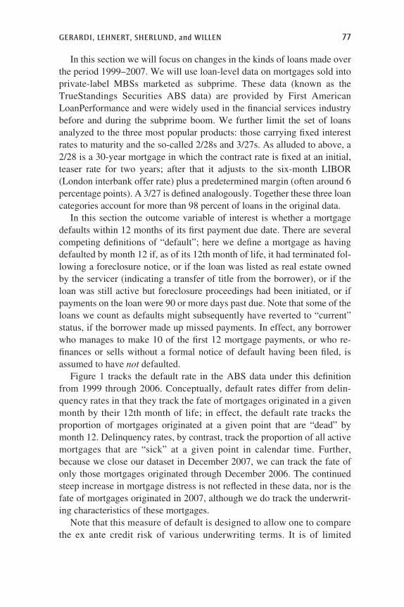
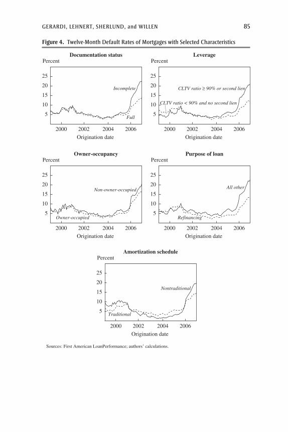
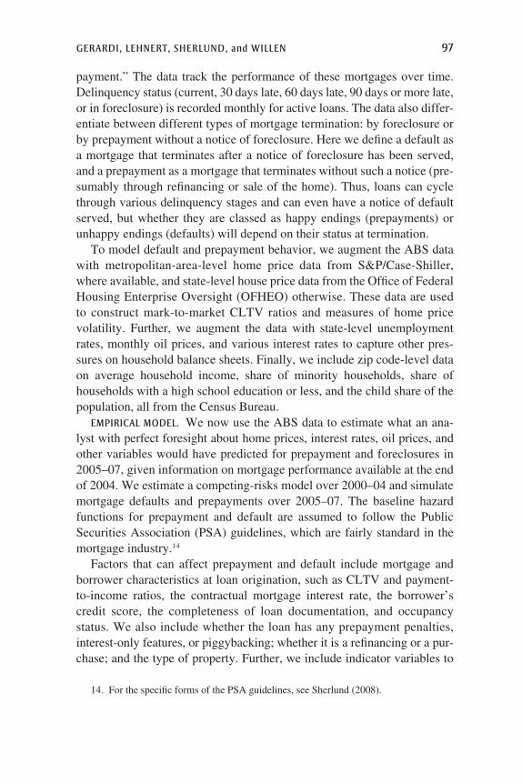
DOCUMENTATION LEVEL. The top left panel of figure 4 shows defaultrates over time for loans with complete and those with incomplete docu-mentation. The two loan types performed roughly in line with one anotheruntil the current cycle, when default rates on loans with incomplete docu-mentation rose far more rapidly than default rates on loans with completedocumentation.
LEVERAGE. The top right panel of figure 4 shows default rates on loanswith and without high CLTV ratios (defined, again, as those with a CLTVratio of at least 90 percent or with a junior lien present at origination).Again, loans with high leverage performed approximately in line withother loans until the most recent episode.
As we highlighted above, leverage is often opaque. To dig deeper intothe correlation between leverage at origination and subsequent perfor-mance, we estimated a pair of simple regressions relating the CLTV ratioat origination to the subsequent probability of default and to the initial con-tract interest rate charged to the borrower. For all loans in the sample, weestimated a probit model of default and an ordinary least squares (OLS)model of the initial contract rate. Explanatory variables were various mea-sures of leverage, including indicator (dummy) variables for variousranges of the reported CLTV ratio (one of which is for a CLTV ratio ofexactly 80 percent) as well as for the presence of a second lien. We esti-mated two versions of each model: version 1 contains only the CLTV ratiomeasures, the second-lien indicator, and (in the default regressions) theinitial contract rate; version 2 adds state and origination date fixed effects.These regressions are designed purely to highlight the correlation amongvariables of interest and not as fully fledged risk models. Version 1 canbe thought of as the simple multivariate correlation across the entire sam-ple, whereas version 2 compares loans originated in the same state at the
84 Brookings Papers on Economic Activity, Fall 2008
11472-02_Gerardi_rev3.qxd 3/6/09 12:24 PM Page 84
GERARDI, LEHNERT, SHERLUND, and WILLEN 85
Sources: First American LoanPerformance; authors’ calculations.
Percent
2004
Origination date
2002 2006
Documentation status
5
10
15
20
25
2000
Percent
2004
Origination date
2002 2006
Leverage
5
10
15
20
25
2000
Percent
2004
Origination date
2002 2006
Owner-occupancy
5
10
15
20
25
2000
Percent
2004
Origination date
2002 2006
Purpose of loan
5
10
15
20
25
2000
CLTV ratio ≥ 90% or second lien
CLTV ratio < 90% and no second lien
Owner-occupied
Non-owner-occupied
Incomplete
Full
Percent
2004
Origination date
2002 2006
Amortization schedule
5
10
15
20
25
2000
Traditional
Nontraditional
Refinancing
All other
Figure 4. Twelve-Month Default Rates of Mortgages with Selected Characteristics
11472-02_Gerardi_rev3.qxd 3/6/09 12:24 PM Page 85

same time. The results are shown in table 3; using the results from ver-sion 2, figure 5 plots the expected default probability against the CLTVratio for loans originated in California in June 2005.
As the figure shows, default probabilities generally increase withleverage. Note, however, that loans with reported CLTV ratios of exactly80 percent, which account for 15.7 percent of subprime loans, have a sub-
86 Brookings Papers on Economic Activity, Fall 2008
Table 3. Regressions Estimating the Effect of Leverage on Default Probability and Mortgage Interest Rates
Marginal effect onprobability of default Marginal effect onwithin 12 months of initial contract
originationa interest rateb
VariableIndependent variable Version 1 Version 2 Version 1 Version 2 meanc
Constant 7.9825 10.4713CLTV ratio (percent) 0.00219 0.00223 0.0093 0.0083 82.6929CLTV2/100 −0.00103 −0.00103 −0.0063 −0.0082 70.3912Initial contract 0.01940 0.02355 8.2037
interest rate (percent a year)
Indicator variablesCLTV ratio = 80 percent 0.00961 0.01036 −0.0127 −0.0817 15.72CLTV ratio between 0.00014 −0.00302 0.0430 0.1106 15.56
80 and 90 percentCLTV ratio = 90 percent 0.00724 −0.00041 0.1037 0.2266 12.86CLTV ratio between 0.00368 −0.00734 0.0202 0.3258 9.68
90 and 100 percentCLTV ratio 100 percent 0.00901 −0.00740 0.0158 0.3777 16.20
or greaterSecond lien recorded 0.05262 0.04500 −0.8522 −0.6491 14.52
Regression includes No Yes No Yesorigination dateeffects
Regression includes No Yes No Yesstate effects
No. of observationsd 679,518 679,518 707,823 707,823Memorandum: mean 6.55
default rate (percent)
Source: Authors’ regressions.a. Results are from a probit regression in which the dependent variable is an indicator equal to 1 when
the mortgage has defaulted by its 12th month.b. Results are from an ordinary least squares regression in which the dependent variable is the original
contract interest rate on the mortgage.c. Values for indicator variables are percent of the total sample for which the variable equals 1.d. Sample is a 10 percent random sample of the ABS data.
11472-02_Gerardi_rev3.qxd 3/6/09 12:24 PM Page 86

stantially higher default probability than loans with slightly higher orlower CLTV ratios. Indeed, under version 2 such loans are among theriskiest originated. As the bottom panel of figure 5 shows, however, thereis no compensating increase in the initial contract rate charged to the bor-rower, although the lender may have charged points and fees up front (notmeasured in this dataset) to compensate for the increased risk. This evi-dence suggests that borrowers with apparently reasonable CLTV ratioswere in fact using junior liens to increase their leverage in a way that wasneither easily visible to investors nor, apparently, compensated by highermortgage interest rates.
GERARDI, LEHNERT, SHERLUND, and WILLEN 87
0.04
0.06
ProbabilityDefault probability
80 100CLTV ratio at origination
CLTV ratio at origination
0.07
0.05
75 85 90 95 105
7.0
8.0
Percent a yearInitial contract interest rate
80 100
7.5
75 85 90 95 105
Version 1
Version 2
Version 1
Version 2
Sources: First American LoanPerformance; authors’ calculations.a. Estimation results of model versions 1 and 2 are reported in table 3.
Figure 5. Effect of CLTV Ratio on Default Probability and Initial Interest Ratea
11472-02_Gerardi_rev3.qxd 3/6/09 12:24 PM Page 87

OTHER RISK FACTORS. The bottom three panels of figure 4 show the defaultrates associated with the three other risk factors described earlier: non-owner-occupancy, loan purpose, and nontraditional amortization sched-ules. Loans to non-owner-occupiers were not (in this sample) markedlyriskier than loans to owner-occupiers. The 12-month default rates on loansoriginated from 1999 to 2004 varied little between those originated forhome purchase and those originated for refinancing, and between thosecarrying traditional and nontraditional amortization schedules. However,among loans originated in 2005 and 2006, purchase loans and loans withnontraditional amortization schedules defaulted at much higher rates thandid refinancings and traditionally amortizing loans, respectively.
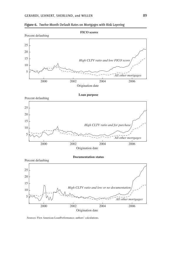
RISK LAYERING. Figure 6 shows the default rates on loans carrying themultiple risk factors discussed earlier. As the top panel shows, loans withhigh CLTV ratios and low FICO scores have nearly always defaulted athigher rates than other loans. High-CLTV-ratio loans that were used topurchase homes also had a worse track record (middle panel). In bothcases, default rates for high-CLTV-ratio loans climbed sharply over thelast two years of the sample. Loans with high CLTV ratios and incompletedocumentation (bottom panel), however, showed the sharpest increase indefaults relative to other loans. This suggests that within the group of high-leverage loans, those with incomplete documentation were particularlyprone to default.
Decomposing the Increase in Defaults
As figure 1 showed, subprime loans originated in 2005 and 2006defaulted at a much higher rate than those originated earlier in the sample.The previous discussion suggests that this increase is not related to observ-able underwriting factors. For example, high-CLTV-ratio loans originatedin 2002 defaulted at about the same rate as other loans originated that sameyear. However, high-CLTV-ratio loans originated in 2006 defaulted atmuch higher rates than other loans.
Decomposing the increase in defaults into a piece due to the mix oftypes of loans originated and a piece due to changes in home pricesrequires data on how all loan types behave under a wide range of price sce-narios. If the loans originated in 2006 were truly novel, there would be nounique decomposition between home prices and underwriting standards.We showed that at least some of the riskiest loan types were being origi-nated (albeit in low numbers) by 2004.
To test this idea more formally, we divide the sample into two groups:an “early” group of loans originated in 1999–2004, and a “late” group
88 Brookings Papers on Economic Activity, Fall 2008
11472-02_Gerardi_rev3.qxd 3/6/09 12:24 PM Page 88
GERARDI, LEHNERT, SHERLUND, and WILLEN 89
5
20
Percent defaultingFICO scores
2006Origination date
25
15
10
5
20
25
15
10
5
20
25
15
10
2000 2002 2004
20062000 2002 2004
2000 2002 2004 2006
Percent defaultingLoan purpose
Origination date
Percent defaultingDocumentation status
Origination date
Sources: First American LoanPerformance; authors’ calculations.
High CLTV ratio and low FICO score
All other mortgages
High CLTV ratio and for purchase
High CLTV ratio and low or no documentation
All other mortgages
All other mortgages
Figure 6. Twelve-Month Default Rates on Mortgages with Risk Layering
11472-02_Gerardi_rev3.qxd 3/6/09 12:24 PM Page 89

originated in 2005 and 2006. We estimate default models separately oneach group, and we track changes in risk factors over the entire period. Wethen measure the changes in risk factors between the two groups and thechanges in the coefficients of the risk model. We find that increases inhigh-leverage lending and risk layering can account for some, but by nomeans all, of the increase in defaults.
Table 4 reports the means of the relevant variables for the two groupsand for the entire sample. The table shows that a much larger fraction ofloans originated in the late group defaulted: 9.28 percent as opposed to4.60 percent in the early group. The differences between the two groups onother risk factors are in line with the earlier discussion: FICO scores,CLTV ratios, the incidence of 2/28s, low-documentation loans, and loanswith nontraditional amortization all rose from the early group to the lategroup, while the share of loans for refinancing fell (implying that the sharefor home purchase rose).
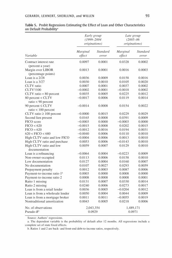
Table 5 reports the results of a loan-level probit model of the probabil-ity of default, estimated using data from the early group and the late group.The table shows marginal effects and standard errors for a number of loanand borrower characteristics; the model also includes a set of state fixedeffects (results not reported). The differences in estimated marginal effectsbetween the early and the late group are striking. Defaults are more sensi-tive in the late group to a variety of risk factors, such as leverage, creditscore, loan purpose, and type of amortization schedule. The slopes intable 5 correspond roughly to the returns in a Blinder-Oaxaca decompo-sition, whereas the sample means in table 4 correspond to the differencesin endowments between the two groups. However, because the underlyingmodel is nonlinear, we cannot perform the familiar Blinder-Oaxacadecomposition.
As a first step toward our decomposition, table 6 reports the predicteddefault rate in the late group using the model estimated on data from theearly group, as well as other combinations. Using early-group coefficientson the early group of loans, the model predicts a 4.60 percent default rate.Using the same coefficients on the late-group data, the model predicts a4.55 percent default rate. Thus, the early-group model does not predict asignificant rise in defaults based on the observable characteristics for thelate group. These results are consistent with the view that a factor otherthan underwriting changes was primarily responsible for the increase inmortgage defaults. However, because these results mix changes in the dis-tribution of risk factors between the two groups as well as changes in theriskiness of certain characteristics, it will be useful to consider the increase
90 Brookings Papers on Economic Activity, Fall 2008
11472-02_Gerardi_rev3.qxd 3/6/09 12:24 PM Page 90

(con
tinu
ed)
Tabl
e 4.
Sum
mar
y St
atis
tics
for
Vari
able
s fr
om th
e AB
S D
ata
Perc
ent o
f to
tal e
xcep
t whe
re s
tate
d ot
herw
ise
All
mor
tgag
esE
arly
gro
upa
Lat
e gr
oupb
Var
iabl
eM
ean
Stan
dard
dev
iati
onM
ean
Stan
dard
dev
iati
onM
ean
Stan
dard
dev
iati
on
Out
com
e 12
mon
ths
afte
r or
igin
atio
nD
efau
lted
6.57
24.7
84.
6020
.95
9.28
29.0
1R
efina
nced
16.2
236
.86
15.9
636
.63
16.5
737
.18
Mor
tgag
e ch
arac
teri
stic
sC
ontr
act i
nter
est r
ate
(per
cent
a y
ear)
8.21
1.59
8.38
1.76
7.97
1.27
Mar
gin
over
LIB
OR
(pe
rcen
tage
poi
nts)
4.45
2.94
4.28
3.11
4.69
2.67
FIC
O s
core
610
6060
761
615
58C
LT
V r
atio
(pe
rcen
t)83
1481
1485
15
Mor
tgag
e ty
peF
ixed
rat
e28
.14
44.9
732
.30
46.7
622
.43
41.7
12/
28c
58.5
449
.27
53.4
049
.88
65.5
847
.51
3/27
13.3
333
.99
14.3
035
.01
11.9
932
.48
Doc
umen
tati
on s
tatu
sC
ompl
ete
68.2
846
.54
70.6
245
.55
65.0
747
.68
No
docu
men
tati
on0.
315.
580.
386.
120.
234.
75L
ow d
ocum
enta
tion
30.7
146
.13
27.8
244
.81
34.6
847
.60
11472-02_Gerardi_rev3.qxd 3/6/09 12:24 PM Page 91

Tabl
e 4.
Sum
mar
y St
atis
tics
for
Vari
able
s fr
om th
e AB
S D
ata
(Con
tinu
ed)
Perc
ent o
f to
tal e
xcep
t whe
re s
tate
d ot
herw
ise
All
mor
tgag
esE
arly
gro
upa
Lat
e gr
oupb
Var
iabl
eM
ean
Stan
dard
dev
iati
onM
ean
Stan
dard
dev
iati
onM
ean
Stan
dard
dev
iati
on
Oth
erN
ontr
adit
iona
l am
orti
zati
ond
16.0
436
.69
6.93
25.4
028
.53
45.1
5N
on-o
wne
r-oc
cupi
ed6.
5724
.78
6.51
24.6
86.
6624
.93
Refi
nanc
ing
67.0
047
.02
70.9
545
.40
61.5
848
.64
Sec
ond
lien
pre
sent
14.5
935
.30
7.50
26.3
424
.32
42.9
0P
repa
ymen
t pen
alty
73.5
544
.11
74.0
043
.87
72.9
344
.43
No.
of
obse
rvat
ions
3,53
2,52
52,
043,
354
1,48
9,17
1
Sour
ces:
Fir
st A
mer
ican
Loa
nPef
orm
ance
; aut
hors
’ ca
lcul
atio
ns.
a. M
ortg
ages
ori
gina
ted
from
199
9 to
200
4.b.
Mor
tgag
es o
rigi
nate
d in
200
5 an
d 20
06.
c. A
30-
year
mor
tgag
e w
ith a
low
initi
al (
“tea
ser”
) ra
te in
the
first
two
year
s; a
3/2
7 is
defi
ned
anal
ogou
sly.
d. A
ny m
ortg
age
that
doe
s no
t com
plet
ely
amor
tize
or th
at d
oes
not a
mor
tize
at a
con
stan
t rat
e.
11472-02_Gerardi_rev3.qxd 3/6/09 12:24 PM Page 92
GERARDI, LEHNERT, SHERLUND, and WILLEN 93
Table 5. Probit Regressions Estimating the Effect of Loan and Other Characteristics on Default Probabilitya
Early group Late group(1999–2004 (2005–06originations) originations)
Marginal Standard Marginal StandardVariable effect error effect error
Contract interest rate 0.0097 0.0001 0.0328 0.0002(percent a year)
Margin over LIBOR 0.0013 0.0001 0.0016 0.0003(percentage points)
Loan is a 2/28 0.0036 0.0009 0.0158 0.0016Loan is a 3/27 0.0030 0.0010 0.0105 0.0020CLTV ratio 0.0007 0.0001 0.0037 0.0002CLTV2/100 −0.0002 0.0001 −0.0018 0.0002CLTV ratio = 80 percent 0.0035 0.0005 0.0225 0.001280 percent < CLTV −0.0017 0.0006 0.0119 0.0014
ratio < 90 percent90 percent ≤ CLTV −0.0014 0.0008 0.0154 0.0022
ratio < 100 percentCLTV ratio ≥ 100 percent −0.0000 0.0015 0.0229 0.0029Second lien present 0.0165 0.0008 0.0391 0.0009FICO score −0.0003 0.0000 −0.0003 0.0000FICO < 620 −0.0015 0.0008 0.0202 0.0015FICO = 620 −0.0012 0.0016 0.0194 0.0031620 < FICO < 680 −0.0040 0.0006 0.0110 0.0010High CLTV ratio and low FICO −0.0004 0.0006 0.0013 0.0010High CLTV ratio and purchase 0.0053 0.0006 −0.0143 0.0010High CLTV ratio and low 0.0059 0.0007 0.0129 0.0010
documentationLoan is a refinancing −0.0064 0.0004 −0.0223 0.0009Non-owner-occupied 0.0113 0.0006 0.0158 0.0010Low documentation 0.0127 0.0004 0.0160 0.0007No documentation 0.0107 0.0027 0.0293 0.0059Prepayment penalty 0.0012 0.0003 0.0087 0.0006Payment-to-income ratio 1b 0.0003 0.0000 0.0008 0.0000Payment-to-income ratio 2 0.0008 0.0008 0.0008 0.0001Ratio 1 missing 0.0131 0.0007 0.0330 0.0014Ratio 2 missing 0.0240 0.0006 0.0273 0.0017Loan is from a retail lender 0.0036 0.0005 −0.0204 0.0012Loan is from a wholesale lender 0.0050 0.0004 0.0044 0.0009Loan is from a mortgage broker 0.0011 0.0011 −0.0055 0.0019Nontraditional amortization 0.0043 0.0005 0.0218 0.0006
No. of observations 2,043,354 1,489,171Pseudo-R2 0.0929 0.0971
Source: Authors’ regressions.a. The dependent variable is the probability of default after 12 months. All regressions include a
complete set of state fixed effects.b. Ratios 1 and 2 are back- and front-end debt-to-income ratios, respectively.
11472-02_Gerardi_rev3.qxd 3/6/09 12:24 PM Page 93

in riskiness of a typical loan after varying a few characteristics in turn.Again, because of the nonlinearity of the underlying model, we have toconsider just one set of observable characteristics at a time.
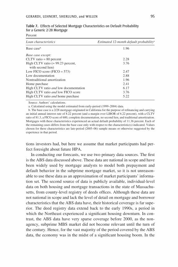
To this end, we consider a typical 2/28 loan originated in Californiawith observable characteristics set to their early-period sample means. Wechange each risk characteristic in turn to its late-period sample mean or toa value suggested by the experience in the late period. Table 7 shows thateven for loans with the worst combination of underwriting characteristics,the predicted default rate is less than half the actual default rate experi-enced by this group of loans. The greatest increases in default probabilityare associated with higher-leverage scenarios. (Note that decreasing theCLTV ratio to exactly 80 percent increases the default probability, for rea-sons discussed earlier.)
What Can We Learn from the 2005 Data?
In this section we focus on whether market participants could reasonablyhave estimated the sensitivity of foreclosures to home price decreases. Weestimate standard competing-risks duration models using data on the per-formance of loans originated through the end of 2004—presumably theinformation set available to lenders as they were making decisions aboutloans originated in 2005 and 2006. We produce out-of-sample forecasts offoreclosures assuming the home price outcomes that the economy actuallyexperienced. Later we address the question of what home price expecta-
94 Brookings Papers on Economic Activity, Fall 2008
Table 6. Predicted Default RatesPercent
Default probability using model estimated on data from
Data used in estimation Early period (1999–2004) Late period (2005–06)
Early period 4.60 9.30Late period 4.55 9.27
Origination year1999 6.66 15.372000 8.67 20.002001 6.52 14.342002 4.83 9.862003 3.49 6.422004 3.44 6.052005 3.96 7.502006 5.31 11.55
Source: Authors’ calculations.
11472-02_Gerardi_rev3.qxd 3/6/09 12:24 PM Page 94
tions investors had, but here we assume that market participants had per-fect foresight about future HPA.
In conducting our forecasts, we use two primary data sources. The firstis the ABS data discussed above. These data are national in scope and havebeen widely used by mortgage analysts to model both prepayment anddefault behavior in the subprime mortgage market, so it is not unreason-able to use these data as an approximation of market participants’ informa-tion set. The second source of data is publicly available, individual-leveldata on both housing and mortgage transactions in the state of Massachu-setts, from county-level registry of deeds offices. Although these data arenot national in scope and lack the level of detail on mortgage and borrowercharacteristics that the ABS data have, their historical coverage is far supe-rior. The deed registry data extend back to the early 1990s, a period inwhich the Northeast experienced a significant housing downturn. In con-trast, the ABS data have very sparse coverage before 2000, as the non-agency, subprime MBS market did not become relevant until the turn ofthe century. Hence, for the vast majority of the period covered by the ABSdata, the economy was in the midst of a significant housing boom. In the
GERARDI, LEHNERT, SHERLUND, and WILLEN 95
Table 7. Effects of Selected Mortgage Characteristics on Default Probability for a Generic 2/28 MortgagePercent
Loan characteristics Estimated 12-month default probabilitya
Base caseb 1.96
Base case except:CLTV ratio = 80 percent 2.28High CLTV ratio (= 99.23 percent, 3.76
with second lien)Low FICO score (FICO = 573) 2.47Low documentation 2.88Nontraditional amortization 1.96Home purchase 2.41High CLTV ratio and low documentation 6.17High CLTV ratio and low FICO score 3.76High CLTV ratio and home purchase 5.22
Source: Authors’ calculations.a. Calculated using the model estimated from early-period (1999–2004) data.b. The base case is a 2/28 mortgage originated in California for the purpose of refinancing and carrying
an initial annual interest rate of 8.22 percent (and a margin over LIBOR of 6.22 percent), with a CLTVratio of 81.3, a FICO score of 600, complete documentation, no second lien, and traditional amortization.Mortgages with these characteristics experienced an actual default probability of 11.36 percent. Each ofthe remaining cases differs from the base case only with respect to the characteristic(s) indicated. Valueschosen for these characteristics are late-period (2005–06) sample means or otherwise suggested by theexperience in that period.
11472-02_Gerardi_rev3.qxd 3/6/09 12:24 PM Page 95

next section we discuss the potential implications of this data limitation forpredicting mortgage defaults and foreclosures.
The Relationship between Housing Equity and Foreclosure
For a homeowner with positive equity who needs to terminate his or hermortgage, a strategy of either refinancing the mortgage or selling the homedominates defaulting and allowing foreclosure to occur. However, for an“underwater” homeowner (that is, one with negative equity, where themortgage balance exceeds the home’s market value), default and foreclo-sure are sometimes the optimal economic decision.13 Thus, the theoreticalrelationship between equity and foreclosure is not linear. Rather, the sensi-tivity of default to equity should be approximately zero for positive valuesof equity, but negative for negative values. These observations imply thatthe relationship between housing prices and foreclosure is highly sensitiveto the housing cycle. In a home price boom, even borrowers in extremefinancial distress have more appealing options than foreclosure, becausehome price gains are expected to result in positive equity. However, whenhome prices are falling, highly leveraged borrowers will often find them-selves in a position of negative equity, which implies fewer options forthose experiencing financial distress.
As a result, estimating the empirical relationship between home pricesand foreclosures requires, in principle, data that span a home price bust aswell as a boom. In addition, analysts using loan-level data must account forthe fact that even as foreclosures rise in a home price bust, prepaymentswill also fall.
Given that the ABS data do not contain a home price bust through theend of 2004, and that, as loan-level data, they could not track the experi-ence of an individual borrower across many loans, we expect (and find)that models estimated using the ABS data through 2004 have a harder timepredicting foreclosures in 2007 and 2008.
Forecasts Using the ABS Data
As described earlier, the ABS data are loan-level data that track mort-gages held in securitized pools marketed as either alt-A or subprime. Werestrict our attention to first-lien, 30-year subprime mortgages originatedfrom 2000 to 2007.
A key difference between the model we estimate in this section and thedecomposition exercise above is in the definitions of “default” and “pre-
96 Brookings Papers on Economic Activity, Fall 2008
13. See Foote and others (2008a) for a more detailed discussion.
11472-02_Gerardi_rev3.qxd 3/6/09 12:24 PM Page 96
payment.” The data track the performance of these mortgages over time.Delinquency status (current, 30 days late, 60 days late, 90 days or more late,or in foreclosure) is recorded monthly for active loans. The data also differ-entiate between different types of mortgage termination: by foreclosure orby prepayment without a notice of foreclosure. Here we define a default asa mortgage that terminates after a notice of foreclosure has been served,and a prepayment as a mortgage that terminates without such a notice (pre-sumably through refinancing or sale of the home). Thus, loans can cyclethrough various delinquency stages and can even have a notice of defaultserved, but whether they are classed as happy endings (prepayments) orunhappy endings (defaults) will depend on their status at termination.
To model default and prepayment behavior, we augment the ABS datawith metropolitan-area-level home price data from S&P/Case-Shiller,where available, and state-level house price data from the Office of FederalHousing Enterprise Oversight (OFHEO) otherwise. These data are usedto construct mark-to-market CLTV ratios and measures of home pricevolatility. Further, we augment the data with state-level unemploymentrates, monthly oil prices, and various interest rates to capture other pres-sures on household balance sheets. Finally, we include zip code-level dataon average household income, share of minority households, share ofhouseholds with a high school education or less, and the child share of thepopulation, all from the Census Bureau.
EMPIRICAL MODEL. We now use the ABS data to estimate what an ana-lyst with perfect foresight about home prices, interest rates, oil prices, andother variables would have predicted for prepayment and foreclosures in2005–07, given information on mortgage performance available at the endof 2004. We estimate a competing-risks model over 2000–04 and simulatemortgage defaults and prepayments over 2005–07. The baseline hazardfunctions for prepayment and default are assumed to follow the PublicSecurities Association (PSA) guidelines, which are fairly standard in themortgage industry.14
Factors that can affect prepayment and default include mortgage andborrower characteristics at loan origination, such as CLTV and payment-to-income ratios, the contractual mortgage interest rate, the borrower’scredit score, the completeness of loan documentation, and occupancystatus. We also include whether the loan has any prepayment penalties,interest-only features, or piggybacking; whether it is a refinancing or a pur-chase; and the type of property. Further, we include indicator variables to
GERARDI, LEHNERT, SHERLUND, and WILLEN 97
14. For the specific forms of the PSA guidelines, see Sherlund (2008).
11472-02_Gerardi_rev3.qxd 3/6/09 12:24 PM Page 97
identify loans with risk layering of high leverage and poor documenta-tion, loans to borrowers with credit scores below 600, and an interactionterm between occupancy status and cumulative HPA over the life of themortgage.
Similarly, we include dynamically updated mortgage and borrowercharacteristics that vary from month to month after loan origination. Themost important of these is an estimate of the mark-to-market CLTV ratio;changes in home prices will primarily affect default and prepayment ratesthrough this variable. In addition, we include the current contract interestrate, home price volatility, state-level unemployment rates, oil prices, and,for ARMs, the fully indexed mortgage interest rate (six-month LIBORplus the loan margin).
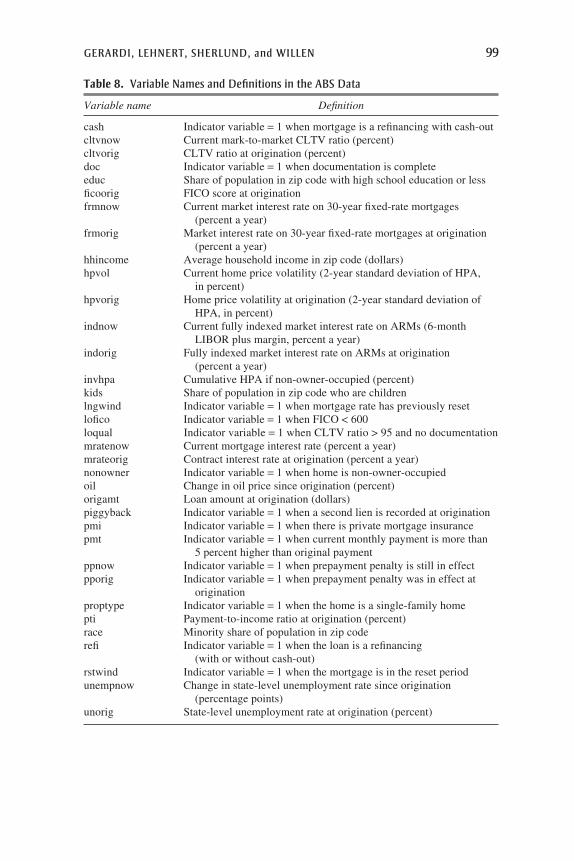
Because of the focus on payment changes, we include three indicatorvariables to capture the effects of interest rate resets. The first is set to unityin the three months around (one month before, the month of, and the monthafter) the first reset. The second captures whether the loan has passed itsfirst reset date. The third identifies changes in the monthly mortgage pay-ment of more than 5 percent from the original monthly payment, to captureany large payment shocks. Variable names and definitions for our modelsusing the ABS data are reported in table 8, and summary statistics in table 9.
ESTIMATION STRATEGY AND RESULTS. We estimate a competing-risks,proportional hazard model for six subsamples of our data. First, the dataare broken down by subprime product type: hybrid 2/28s, hybrid 3/27s,and fixed-rate mortgages. Second, for each product type, estimation iscarried out separately for purchase mortgages and refinancings.
Table 10 reports the estimation results for the default hazard functions.15
These results are similar to those previously reported by Sherlund.16 As onewould expect, home prices (acting through the mark-to-market CLTV ratioterm) are extremely important. In addition, non-owner-occupiers are, allelse equal, likelier to default. The payment shock and reset window vari-ables have relatively small effects, possibly because so many subprimeborrowers defaulted in 2006 and 2007 ahead of their resets. Aggregatevariables such as oil prices and unemployment rates do push up defaults,but by relatively small amounts, once we control for loan-level observables.
SIMULATION RESULTS. With the estimated parameters in hand, we turn tothe question of how well the model performs over the 2005–07 period.
98 Brookings Papers on Economic Activity, Fall 2008
15. For brevity we do not report the parameter estimates for the prepayment hazardfunctions. They are available upon request from the authors.
16. Sherlund (2008).
11472-02_Gerardi_rev3.qxd 3/6/09 12:24 PM Page 98
GERARDI, LEHNERT, SHERLUND, and WILLEN 99
Table 8. Variable Names and Definitions in the ABS Data
Variable name Definition
cash Indicator variable = 1 when mortgage is a refinancing with cash-outcltvnow Current mark-to-market CLTV ratio (percent)cltvorig CLTV ratio at origination (percent)doc Indicator variable = 1 when documentation is completeeduc Share of population in zip code with high school education or lessficoorig FICO score at originationfrmnow Current market interest rate on 30-year fixed-rate mortgages
(percent a year)frmorig Market interest rate on 30-year fixed-rate mortgages at origination
(percent a year)hhincome Average household income in zip code (dollars)hpvol Current home price volatility (2-year standard deviation of HPA,
in percent)hpvorig Home price volatility at origination (2-year standard deviation of
HPA, in percent)indnow Current fully indexed market interest rate on ARMs (6-month
LIBOR plus margin, percent a year)indorig Fully indexed market interest rate on ARMs at origination
(percent a year)invhpa Cumulative HPA if non-owner-occupied (percent)kids Share of population in zip code who are childrenlngwind Indicator variable = 1 when mortgage rate has previously resetlofico Indicator variable = 1 when FICO < 600loqual Indicator variable = 1 when CLTV ratio > 95 and no documentationmratenow Current mortgage interest rate (percent a year)mrateorig Contract interest rate at origination (percent a year)nonowner Indicator variable = 1 when home is non-owner-occupiedoil Change in oil price since origination (percent)origamt Loan amount at origination (dollars)piggyback Indicator variable = 1 when a second lien is recorded at originationpmi Indicator variable = 1 when there is private mortgage insurancepmt Indicator variable = 1 when current monthly payment is more than
5 percent higher than original paymentppnow Indicator variable = 1 when prepayment penalty is still in effectpporig Indicator variable = 1 when prepayment penalty was in effect at
originationproptype Indicator variable = 1 when the home is a single-family homepti Payment-to-income ratio at origination (percent)race Minority share of population in zip coderefi Indicator variable = 1 when the loan is a refinancing
(with or without cash-out)rstwind Indicator variable = 1 when the mortgage is in the reset periodunempnow Change in state-level unemployment rate since origination
(percentage points)unorig State-level unemployment rate at origination (percent)
11472-02_Gerardi_rev3.qxd 3/6/09 12:24 PM Page 99

Tabl
e 9.
Sam
ple
Aver
ages
of V
aria
bles
in th
e AB
S D
ataa
2000
–04
2004
2005
Var
iabl
e na
me
At o
rigi
nati
onA
ctiv
e m
ortg
ages
Mor
tgag
es in
def
ault
Mor
tgag
es p
repa
idA
t ori
gina
tion
At o
rigi
nati
on
cash
0.57
0.57
0.52
0.58
0.58
0.54
cltv
now
81.9
173
.59
66.1
00.
0083
.76
84.9
0cl
tvor
ig81
.91
83.1
581
.61
79.8
183
.76
84.9
0do
c0.
700.
690.
740.
700.
660.
64ed
uc0.
360.
370.
380.
350.
370.
37fi
coor
ig61
061
658
260
561
661
9fr
mno
w6.
285.
755.
755.
755.
885.
85fr
mor
ig6.
286.
036.
896.
625.
885.
85hh
inco
me
43,1
1042
,421
39,1
1644
,945
43,0
0742
,379
hpvo
l3.
384.
153.
204.
783.
914.
57hp
vori
g3.
383.
412.
523.
463.
914.
57in
dnow
8.52
9.06
9.51
9.12
7.90
9.81
indo
rig
8.52
8.06
10.0
69.
057.
909.
81in
vhpa
1.63
1.14
2.31
2.38
0.55
0.16
kids
0.27
0.27
0.27
0.27
0.27
0.27
lngw
ind
0.00
0.09
0.20
0.11
0.00
0.00
loqu
al0.
050.
070.
030.
030.
090.
12m
rate
now
8.22
7.73
9.95
8.81
7.32
7.56
mra
teor
ig8.
227.
729.
958.
827.
327.
56
11472-02_Gerardi_rev3.qxd 3/6/09 12:24 PM Page 100

nono
wne
r0.
080.
090.
100.
070.
090.
08oi
l0.
0026
.96
54.4
753
.35
0.00
0.00
orig
amt
118,
523
119,
569
89,0
9612
1,63
613
6,19
214
8,32
0pi
ggyb
ack
0.08
0.11
0.05
0.04
0.14
0.23
pmi
0.27
0.24
0.35
0.31
0.19
0.23
pmt
0.00
0.04
0.03
0.00
0.00
0.00
ppno
w0.
730.
670.
360.
380.
730.
72pp
orig
0.73
0.74
0.75
0.71
0.73
0.72
prop
type
0.87
0.88
0.90
0.86
0.87
0.86
pti
38.9
938
.87
39.0
939
.18
39.4
140
.07
race
0.31
0.30
0.32
0.31
0.31
0.31
refi
0.68
0.67
0.64
0.70
0.65
0.60
rstw
ind
0.00
0.02
0.06
0.09
0.00
0.00
unem
pnow
0.00
−4.5
013
.47
2.95
0.00
0.00
unor
ig5.
585.
695.
065.
485.
635.
06
No.
of
obse
rvat
ions
3,65
4,68
32,
195,
233
183,
586
1,27
5,86
41,
267,
866
1,79
4,95
3
Sour
ce: A
utho
rs’
calc
ulat
ions
.a.
See
tabl
e 8
for
vari
able
defi
nitio
ns.
11472-02_Gerardi_rev3.qxd 3/6/09 12:24 PM Page 101

Tabl
e 10
.D
efau
lt H
azar
d Fu
nctio
n Es
timat
es fr
om th
e AB
S D
ata,
200
0–04
a
Subp
rim
e 2/
28Su
bpri
me
3/27
Subp
rim
e fix
ed-r
ate
Var
iabl
e na
me
Pur
chas
eR
efina
ncin
gP
urch
ase
Refi
nanc
ing
Pur
chas
eR
efina
ncin
g
Con
stan
t7.
519*
4.14
3*5.
819*
−0.8
427.
826*
3.21
3*ca
shN
Ab
0.01
6N
A0.
087
NA
−0.1
10*
cltv
now
0.03
0*0.
008*
0.01
9*0.
025*
0.03
6*0.
028*
cltv
orig
−0.0
32*
0.00
2−0
.010
−0.0
08−0
.027
*−0
.011
*do
c−0
.185
*−0
.378
*−0
.012
−0.2
72*
−0.2
71*
−0.1
94*
educ
−0.4
39−0
.125
−1.4
01*
−0.3
76−0
.075
0.22
7fi
coor
ig−4
.388
*−4
.881
*−4
.084
*−2
.321
*−4
.874
*−4
.386
*fr
mno
w−0
.124
*−0
.179
*0.
054
0.10
90.
181*
0.11
3*fr
mor
ig−0
.105
*0.
105*
−0.3
10*
−0.0
25−0
.209
*−0
.198
*hh
inco
me
−0.5
75*
−0.2
56*
−0.7
58*
−0.2
23−0
.872
*−0
.222
*hp
vol
−0.0
34*
−0.0
38*
−0.0
46*
−0.0
29−0
.064
*−0
.037
*in
dnow
0.29
1*0.
369*
0.21
7*0.
234*
NA
NA
indo
rig
−0.2
70*
−0.3
58*
−0.1
36*
−0.1
45*
NA
NA
invh
pa−0
.032
*−0
.012
*−0
.064
*−0
.015
−0.0
30*
−0.0
11*
kids
0.31
70.
249
1.30
4−0
.635
0.52
1−0
.695
lngw
ind
0.13
90.
059
0.68
3*−0
.027
NA
NA
lofi
co−0
.151
*−0
.056
−0.2
56*
0.05
6−0
.085
0.12
8*lo
qual
−0.0
39−0
.112
0.03
1−0
.331
−0.2
150.
561*
mra
teno
w−0
.031
0.04
41.
071*
0.37
60.
468
0.10
9
11472-02_Gerardi_rev3.qxd 3/6/09 12:24 PM Page 102

mra
teor
ig0.
325*
0.27
3*−0
.786
−0.0
67−0
.255
0.15
9no
now
ner
0.55
7*0.
281*
0.88
3*0.
351*
0.54
0*0.
431*
oil
0.00
20.
000
0.00
1−0
.001
0.00
6*0.
005*
orig
amt
0.29
8*0.
115*
0.48
9*0.
234*
0.48
0*0.
148*
pigg
ybac
k0.
287*
0.28
6*0.
300*
0.28
70.
133
−0.3
29pm
i0.
075*
0.17
4*0.
212*
0.07
40.
311*
0.16
0*pm
t0.
525*
−0.1
491.
478*
0.70
7*1.
144*
0.39
3pp
now
−0.1
56*
−0.0
560.
148
−0.0
84−0
.141
−0.3
20*
ppor
ig0.
033
0.11
5−0
.329
0.05
60.
157
0.43
9*pr
opty
pe0.
143*
0.03
10.
167
0.06
0−0
.128
−0.0
25pt
i0.
005*
0.00
9*0.
009*
0.00
7*−0
.002
0.00
6*ra
ce0.
690*
−0.3
02*
0.18
2−0
.082
0.59
3*−0
.324
*rs
twin
d−0
.239
*−0
.150
*0.
100
0.14
3N
AN
Aun
empn
ow0.
007*
0.00
9*0.
005*
0.00
40.
000
−0.0
03*
unor
ig−0
.023
−0.0
40*
−0.0
28−0
.043
−0.0
80−0
.091
*
Log
-lik
elih
ood
−140
,135
−297
,352
−30,
071
−50,
544
−36,
574
−170
,927
No.
of
obse
rvat
ions
1,09
5,22
72,
015,
104
241,
511
373,
976
324,
431
1,58
2,14
6
Sour
ce: A
utho
rs’
calc
ulat
ions
.a.
Coe
ffici
ent e
stim
ates
are
for t
he d
efau
lt ha
zard
func
tion
from
a c
ompe
ting-
risk
s du
ratio
n m
odel
. The
mod
el is
est
imat
ed a
t a m
onth
ly fr
eque
ncy
usin
g th
e m
axim
um li
ke-
lihoo
d m
etho
d. A
ster
isks
indi
cate
sta
tistic
al s
igni
fican
ce a
t the
5 p
erce
nt le
vel.
b. N
A, n
ot a
pplic
able
.
11472-02_Gerardi_rev3.qxd 3/6/09 12:24 PM Page 103
Here we focus on the 2004 and 2005 vintages of subprime mortgages con-tained in the ABS data. To construct the forecasts, we use the estimatedmodel parameters to calculate predicted foreclosure (and prepayment)probabilities for each mortgage in each month during 2005–07. Thesesimulations assume perfect foresight, in that the assumed paths for homeprices, unemployment rates, oil prices, and interest rates follow those thatactually occurred. The average default propensity each month is used todetermine the number of defaults each month, with mortgages with thehighest propensities defaulting first (and similarly for prepayments). Wethen compare the cumulative incidence of simulated defaults with theactual incidence of defaults using cumulative default functions (that is,the percent of original loans that default by loan age t).
The 2004 and 2005 vintages differ on many dimensions: underwritingstandards, the geographic mix of loans originated, oil price shocks experi-enced, and so on. However, the key difference is in the fraction of activeloans in each vintage that experienced the home price bust that started, insome regions, as early as 2006. Loans from both vintages were tied toproperties whose prices declined; however, loans from the later vintagewere much more exposed. As we show, cumulative defaults on the 2004vintage were reasonable, but those on the 2005 vintage skyrocketed. Thus,the comparison of the 2004 and 2005 vintages provides a tougher test of amodel’s ability to predict defaults. Any differences we find here would belarger when comparing vintages further apart; for example, the 2003 vin-tage experienced much greater and more sustained home price gains thandid the 2006 vintage.
Figure 7 displays the results of this vintage simulation exercise. Themodel overpredicts defaults among the 2004 vintage and underpredictsdefaults among the 2005 vintage. It estimates that after 36 months, 9.3 per-cent of the 2005 vintage would have defaulted, but only 7.9 percent of the2004 vintage, an increase of 18 percent. Although this is fairly significant,it is dwarfed by the actual increase in defaults between vintages, bothbecause the 2005 vintage performed so poorly, and because the 2004 vin-tage performed better than expected.
Cash flows from a pool of mortgages are greatly affected by prepay-ments. Loans that are prepaid (because the underlying borrower refinancedor moved) deliver all unpaid principal to the lender, as well as, in somecases, prepayment penalties. Further, loans that are prepaid are not at riskfor future defaults. As the bottom panel of figure 7 shows, predicted pre-payment rates fell dramatically from the 2004 to the 2005 vintage. Themodel predicted that 68 percent of loans originated in 2004, but only
104 Brookings Papers on Economic Activity, Fall 2008
11472-02_Gerardi_rev3.qxd 3/6/09 12:24 PM Page 104

57 percent of loans originated in 2005, would have prepaid by month 36, a16 percent drop. Thus, the simulations predict an 18 percent increase incumulative defaults and a 16 percent drop in cumulative prepayments forthe 2005 vintage of loans relative to the 2004 vintage. These swings wouldhave had a large impact on the cash flows from the pool of loans.
To further investigate the effect of home prices on the model estimatedhere, we compute the conditional default and prepayment rates for the
GERARDI, LEHNERT, SHERLUND, and WILLEN 105
5
Percent of loans (cumulative)Defaults
Months after origination
15
10
6 12 18 24 30
Sources: First American LoanPerformance; authors’ calculations.a. Simulations assume perfect foresight about home prices, interest rates, oil prices, and unemployment rates.
2004 actual2004 simulation
2005 actual
2005 simulation
20
Percent of loans (cumulative)Prepayments
Months after origination
60
50
40
30
10
6 12 18 24 30
2004 actual
2004 simulation
2005 actual
2005 simulation
Figure 7. Default and Prepayment Simulations for the 2004 and 2005 MortgageVintages Using ABS Dataa
11472-02_Gerardi_rev3.qxd 3/6/09 12:24 PM Page 105

generic hybrid 2/28 mortgage analyzed in table 7. By focusing on a partic-ular mortgage type, we eliminate the potentially confounding effects ofchanges in the mix of loans originated, oil prices, interest rates, and so onbetween the two vintages and isolate the pure effect of home prices. We lethome prices, oil prices, unemployment rates, and so on proceed as they didin 2004–06. We then keep everything else constant but replace 2004–06home prices with their 2006–08 trajectories. The resulting conditionaldefault and prepayment rates are shown in figure 8. For this type of mort-gage at least, the sensitivity to home price changes is extreme. The gapbetween the default probabilities increases over time because, again, homeprices operate through the mark-to-market CLTV ratio, and this particularloan started with a CLTV ratio at origination of just over 80 percent. Thegyrations in default and prepayment probabilities around month 24 areassociated with the loan’s first interest rate reset.
Forecasts Using the Registry of Deeds Data
In this subsection we use data from the Warren Group, which collectsmortgage and housing transaction data from Massachusetts registry ofdeeds offices, to analyze the foreclosure crisis in Massachusetts and todetermine whether a researcher armed with these data at the end of 2004could have successfully predicted the rapid rise in foreclosures that fol-lowed. We focus on the state of Massachusetts mostly because of dataavailability. The Warren Group currently collects deed registry data formany of the Northeastern states, but their historical coverage of foreclo-sures is limited to Massachusetts. However, the underlying micro-levelhousing and mortgage historical data are publicly available in many states,and a motivated researcher certainly could have obtained the data had he orshe been inclined to do so before the housing crisis occurred. Indeed, sev-eral vendors sell such data in an easy-to-use format for many states, albeitat significant cost.
The deed registry data include every residential sale deed, includingforeclosure deeds, as well as every mortgage originated in the state ofMassachusetts from January 1990 through December 2007. The data con-tain transaction amounts and dates for mortgages and property sales, butnot mortgage terms or borrower characteristics. The data do identify themortgage lender, which enables us to construct indicators for mortgagesoriginated by subprime lenders.
These data allow us to construct a panel dataset of homeowners, each ofwhom we can follow from the date when they purchase the home to the datewhen they either sell the home, experience a foreclosure, or reach the end
106 Brookings Papers on Economic Activity, Fall 2008
11472-02_Gerardi_rev3.qxd 3/6/09 12:24 PM Page 106

GERARDI, LEHNERT, SHERLUND, and WILLEN 107
0.2
Conditional probability (percent)Defaults
Months after origination
1.0
1.2
0.8
0.6
0.4
6 12 18 24
Source: Authors’ calculations using the model described in the text.a. Probabilities are those in month t conditional on surviving to month t – 1, estimated for a generic 2/28
subprime mortgage with the characteristics described in the base case in table 7. It is assumed that all dynamic variables follow their 2004–06 trajectories except for home prices, which follow either their 2004–06 or their 2006–08 trajectories as indicated.
5
Conditional probability (percent)Prepayments
Months after origination
15
10
6 12 18 24
Using 2004–06 prices
Using 2004–06 prices
Using 2006–08 prices
Using 2006–08 prices
Figure 8. Effect of Changing Home Prices on a Generic 2/28 Mortgagea
11472-02_Gerardi_rev3.qxd 3/6/09 12:24 PM Page 107

of our sample. We use the term “ownership experience” to refer to this timeperiod.17 Since the data include all residential sale transactions, we are alsoable to construct a collection of town-level, quarterly, weighted repeat-sales indexes using the methodology of Karl Case and Robert Shiller.18
We use a slightly different definition of foreclosure in the deed registrydata than in the loan-level analysis above. Here we identify foreclosurethrough the existence of a foreclosure deed, which signifies the very end ofthe foreclosure process, when the property is sold at auction to a privatebidder or to the mortgage lender. This definition is not possible in the loan-level analysis, in part because state foreclosure laws vary greatly, resultingin significant heterogeneity in the time span between the beginning of theforeclosure process and the end.
COMPARISON WITH THE ABS DATA. The deed registry data differ signifi-cantly from the ABS data. Whereas the latter track individual mortgagesover time, the deed registry data track homeowners in the same residenceover time. Thus, with the deed registry data, the researcher can follow thesame homeowner across different mortgages in the same residence anddetermine the eventual outcome of the ownership experience. In contrast,with the ABS data, if the mortgage terminated in a manner other thanforeclosure, such as a refinancing or sale of the property, the borrowerdrops out of the dataset, and the outcome of the ownership experience isunknown. Gerardi, Shapiro, and Willen argue that analyzing ownershipexperiences rather than individual mortgages has certain advantages,depending on the question being addressed.19
As already noted, another major difference between the deed registrydata and the ABS data is the period of coverage. The deed registry dataencompass the housing bust of the early 1990s in the Northeast, in whichthere was a sharp decrease in nominal home prices as well as a significantforeclosure crisis. Figure 9 tracks HPA and the foreclosure rate in Massa-chusetts since 1987. Foreclosure deeds began to rise rapidly starting in1991 and peaked in 1992 at approximately 9,300 statewide. The fore-closure rate remained high through the mid-1990s, until nominal HPAbecame positive in the late 1990s. The housing boom of the early 2000s is
108 Brookings Papers on Economic Activity, Fall 2008
17. See Gerardi, Shapiro, and Willen (2007) for more details regarding the constructionof the dataset.
18. Many Massachusetts towns are too small to allow the construction of precise homeprice indexes. To deal with this issue, we group the smaller towns together based on bothgeographic and demographic criteria. Altogether, we are able to estimate just over 100 indexes for the state’s 350 cities and towns.
19. Gerardi, Shapiro, and Willen (2007).
11472-02_Gerardi_rev3.qxd 3/6/09 12:24 PM Page 108

evident, with double-digit annual HPA and extremely few foreclosures.We see evidence of the current foreclosure crisis at the very end of oursample: the number of foreclosure deeds begins rising in 2006 and by 2007is approaching the levels witnessed in the early 1990s.
The final major difference between the two data sources is in their cov-erage of the subprime mortgage market. Since the ABS data encompass
GERARDI, LEHNERT, SHERLUND, and WILLEN 109
0.2
Percent of all homesForeclosure ratea
0.6
0.4
1995 2000 2005
Sources: Warren Group; Massachusetts Department of Revenue.a. Total foreclosures in a given quarter divided by the total number of residential parcels that year, where a
parcel is any real unit of property used for the assessment of property taxes, and typically consists of a plot of land defined by a deed and any buildings on that land.
b. Calculated using the Case-Shiller weighted, repeat-sales methodology.
1990
1995 2000 20051990
140
Index, 1987Q1 = 100Home pricesb
220
200
180
160
120
100
80
Cyclical peak
Figure 9. Massachusetts Foreclosure Rate and Home Prices, 1987–2007
11472-02_Gerardi_rev3.qxd 3/6/09 12:24 PM Page 109

pools of nonagency MBSs, a subprime mortgage is defined simply as anymortgage contained in a pool of mortgages labeled “subprime.” The deedregistry data do not reveal whether a mortgage is securitized or not, andthus, we cannot use the same subprime definition. Instead, we match eachlender against a list of lenders who originate mainly subprime mortgages;the list is constructed by the Department of Housing and Urban Develop-ment (HUD) on an annual basis. The two definitions are largely consistentwith each other.20 Table 11 shows the top ten Massachusetts subprimelenders for each year going back to 1999, as well as the number of subprimeloans originated by each lender and by all lenders. The composition of thelist does change from year to year, but for the most part the same lendersconsistently occupy a spot on the list. It is evident from the table that sub-prime lending in Massachusetts peaked in 2005 and fell sharply in 2007.The increasing importance of the subprime purchase mortgage market isalso very clear. From 1999 to 2001 the subprime market consisted mostlyof refinancings: in 1999 and 2000 home purchases with subprime mort-gages made up only about 25 percent of the Massachusetts subprime mar-ket, and only about 30 percent in 2001. By 2004, however, purchases madeup almost 78 percent of the subprime mortgage market, and in 2006 theyaccounted for 96 percent. This is certainly evidence supporting the ideathat over time the subprime mortgage market opened up the opportunity ofhomeownership to many households, at least in the state of Massachusetts.
EMPIRICAL MODEL. The empirical model we implement is drawn fromGerardi, Shapiro, and Willen and resembles previous models of mortgagetermination.21 It is a duration model similar to the one used in the aboveanalysis of the ABS data, with a few important differences. As in the loan-level analysis, we use a competing-risks, proportional hazard specification,which assumes that certain baseline hazards are common to all ownershipexperiences. However, because we are now analyzing ownership experi-ences rather than individual loans, the competing risks correspond to thetwo possible terminations of an ownership experience, sale and foreclo-sure, as opposed to the two possible terminations of a mortgage, prepay-ment and foreclosure. As discussed above, the major difference betweenthe two specifications comes in the treatment of refinancings. In the loan-level analysis, a loan that is refinanced drops out of the dataset, because the
110 Brookings Papers on Economic Activity, Fall 2008
20. See Gerardi, Shapiro, and Willen (2007) for a more detailed comparison of differentsubprime mortgage definitions. Mayer and Pence (2008) also compare subprime definitionsand reach similar conclusions.
21. Gerardi, Shapiro, and Willen (2007). Previous models include those of Deng, Quigley,and van Order (2000), Deng and Gabriel (2006), and Pennington-Cross and Ho (2006).
11472-02_Gerardi_rev3.qxd 3/6/09 12:24 PM Page 110

mortgage is terminated. However, in the ownership experience analysis, aborrower who refinances remains in the data. Thus, a borrower whodefaults on a refinanced mortgage will show up as a foreclosure in the deedregistry dataset, but that borrower’s first mortgage will show up in theABS data as a prepayment, and the second mortgage may or may not showup in the data at all (depending on whether the mortgage was sold into aprivate-label MBS), but either way, the two mortgages will not be linkedtogether. Thus, for a given number of eventual foreclosures, the ABS datawill always show a lower apparent foreclosure rate.
Unlike for mortgage terminations, there is no generally accepted stan-dard baseline hazard for ownership terminations. Thus, we specify boththe foreclosure and the sale baseline hazards in a nonparametric manner,using an indicator variable for each year after the purchase of the home. Ineffect, we model the baseline hazards with a set of age dummies.22
The list of explanatory variables is different from that in the loan-levelanalysis. We have detailed information regarding the CLTV ratio at thetime of purchase for each homeowner in the data, and we include theCLTV ratio as a right-hand-side variable. We also combine the initialCLTV ratio with cumulative HPA experienced since purchase in the townwhere the home is located, to construct a measure of household equity, Eit:
where CLTVi0 corresponds to household i’s initial CLTV ratio, and C jtHPA
corresponds to the cumulative amount of HPA experienced in town j fromthe date of the home purchase through time t.23 Based on our discussionabove of the theory of default, an increase in equity for a borrower in aposition of negative nominal home equity should have a significantly dif-ferent effect from an increase in equity for a borrower with positive nomi-nal equity. For this reason we assume a specification that allows the effectof equity on default to change depending on the borrower’s equity. To do
( ) ,11 0
0
EC CLTV
CLTVit
jtHPA
i
i
=+( ) −
GERARDI, LEHNERT, SHERLUND, and WILLEN 111
22. Gerardi, Shapiro, and Willen (2007) and Foote, Gerardi, and Willen (2008) use athird-order polynomial in the age of the ownership. The nonparametric specification usedhere has the advantage of not being affected by the nonlinearities in the tails of the polyno-mials for old ownerships, but the results for both specifications are very similar.
23. This equity measure is somewhat crude as it does not take into account amortization,cash-out refinancings, or home improvements. See Foote and others (2008a) for a moredetailed discussion of the implications of these omissions for the estimates.
11472-02_Gerardi_rev3.qxd 3/6/09 12:24 PM Page 111

Tabl
e 11
.To
p 10
Sub
prim
e Le
nder
s in
Mas
sach
uset
ts, 1
999–
2007
Tot
alP
urch
ase
Tot
alP
urch
ase
Tot
alP
urch
ase
Len
der
orig
inat
ions
orig
inat
ions
Len
der
orig
inat
ions
orig
inat
ions
Len
der
orig
inat
ions
orig
inat
ions
2007
2004
2001
Sum
mit
1,60
11,
584
Opt
ion
One
3,76
73,
129
Opt
ion
One
2,66
01,
111
Opt
ion
One
360
358
New
Cen
tury
2,99
12,
507
New
Cen
tury
1,26
332
3E
quifi
rst
195
195
Fre
emon
t2,
895
2,46
1A
mer
ique
st1,
984
296
New
Cen
tury
149
149
Arg
ent
2,20
02,
068
Cit
ifina
ncia
l Ser
vice
s1,
040
140
Fre
emon
t10
810
7F
ield
ston
e1,
131
1,02
3F
reem
ont
748
317
Acc
redi
ted
Hom
e75
74A
ccre
dite
d H
ome
1,01
482
0H
ouse
hold
Fin
anci
al C
orp.
548
61A
rgen
t73
73M
ortg
age
Len
der
Net
972
536
Wel
ls F
argo
Fin
ance
467
43A
egis
5453
Nat
ion
One
946
927
Arg
ent
457
66W
ilm
ingt
on F
inan
ce46
43W
MC
888
586
Fir
st F
rank
lin
367
251
Nat
ion
One
4444
Lon
g B
each
812
685
Mer
itag
e34
933
3T
otal
a3,
021
2,95
6T
otal
23,7
6118
,481
Tot
al15
,308
4,59
5
2006
2003
2000
Mor
tgag
e L
ende
r N
et2,
489
2,31
0O
ptio
n O
ne3,
157
2,22
2O
ptio
n O
ne2,
773
1,00
0S
umm
it2,
021
1,94
8N
ew C
entu
ry1,
694
1,05
3A
mer
ique
st2,
047
287
Fre
emon
t2,
016
1,97
3F
reem
ont
1,51
91,
089
Cit
ifina
ncia
l Ser
vice
s1,
275
112
New
Cen
tury
1,97
81,
942
Am
eriq
uest
1,28
843
6N
ew C
entu
ry1,
251
336
WM
C1,
888
1,86
0F
irst
Fra
nkli
n92
291
7F
reem
ont
773
267
Opt
ion
One
1,61
61,
552
Arg
ent
836
536
Hou
seho
ld F
inan
cial
Cor
p76
155
Acc
redi
ted
Hom
e1,
006
986
Mor
tgag
e L
ende
r N
et80
238
1L
ong
Bea
ch47
028
9A
rgen
t64
062
6A
ccre
dite
d H
ome
636
428
Fir
st F
rank
lin
464
407
Sou
thst
ar63
262
4F
ield
ston
e58
543
0M
ortg
age
Len
der
Net
464
36E
quifi
rst
598
564
Cit
ifina
ncia
l Ser
vice
s45
970
Arg
ent
437
48T
otal
18,2
1117
,489
Tot
al17
,988
11,0
62T
otal
15,8
703,
982
11472-02_Gerardi_rev3.qxd 3/6/09 12:24 PM Page 112
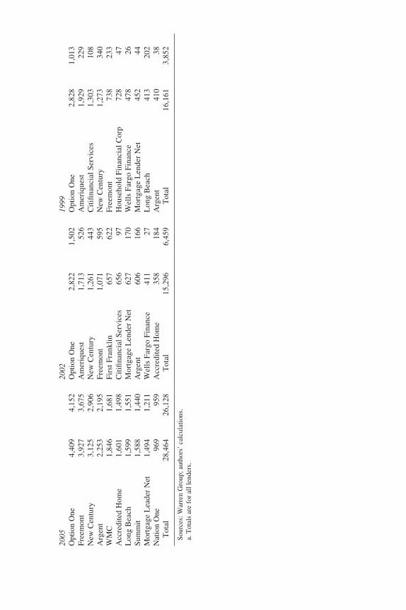
2005
2002
1999
Opt
ion
One
4,40
94,
152
Opt
ion
One
2,82
21,
502
Opt
ion
One
2,82
81,
013
Fre
emon
t3,
927
3,67
5A
mer
ique
st1,
713
526
Am
eriq
uest
1,92
922
9N
ew C
entu
ry3,
125
2,90
6N
ew C
entu
ry1,
261
443
Cit
ifina
ncia
l Ser
vice
s1,
303
108
Arg
ent
2,25
32,
195
Fre
emon
t1,
071
595
New
Cen
tury
1,27
334
0W
MC
1,84
61,
681
Fir
st F
rank
lin
657
622
Fre
emon
t73
823
3A
ccre
dite
d H
ome
1,60
11,
498
Cit
ifina
ncia
l Ser
vice
s65
697
Hou
seho
ld F
inan
cial
Cor
p72
847
Lon
g B
each
1,59
91,
551
Mor
tgag
e L
ende
r N
et62
717
0W
ells
Far
go F
inan
ce47
826
Sum
mit
1,58
81,
440
Arg
ent
606
166
Mor
tgag
e L
ende
r N
et45
244
Mor
tgag
e L
eade
r N
et1,
494
1,21
1W
ells
Far
go F
inan
ce41
127
Lon
g B
each
413
202
Nat
ion
One
969
959
Acc
redi
ted
Hom
e35
818
4A
rgen
t41
038
Tot
al28
,464
26,1
28T
otal
15,2
966,
459
Tot
al16
,161
3,85
2
Sour
ces:
War
ren
Gro
up; a
utho
rs’
calc
ulat
ions
.a.
Tot
als
are
for
all l
ende
rs.
11472-02_Gerardi_rev3.qxd 3/6/09 12:24 PM Page 113
this we specify equity as a linear spline with six intervals: (−∞, −10%),[−10%, 0%), [0%, 10%), [10%, 25%), and [25%, ∞).24
Since detailed mortgage and borrower characteristics are not availablein the deed registry data, we instead use zip code–level demographic infor-mation from the 2000 Census, including median household income and thepercentage of minority households in the zip code, and town-level un-employment rates from the Bureau of Labor Statistics. We also includethe six-month LIBOR in the list of explanatory variables, to capture theeffects of nominal interest rates on sale and foreclosure.25 Finally, weinclude an indicator variable for whether the homeowner obtained financ-ing from a lender on the HUD subprime lender list at the time of purchase.This variable is included as a proxy for the different mortgage and bor-rower characteristics that distinguish the subprime from the prime mort-gage market. We emphasize that we do not assign a causal interpretation tothis variable. Rather we interpret the estimated coefficient as a correlationthat simply reveals the relative frequency of foreclosure for a subprimepurchase borrower compared with a borrower who has a prime mortgage.
Table 12 reports summary statistics for the number of new Massachu-setts ownership experiences initiated, and the number of sales and fore-closures broken down by vintage. The two most recent housing cyclesare clearly evident. Almost 5 percent of ownerships initiated in 1990, butfewer than 1 percent of those in vintages between 1996 and 2002, eventu-ally experienced a foreclosure. Despite a severe right-censoring problemfor the 2005 vintage of ownerships, as of December 2007 more than 2 per-cent had already succumbed to foreclosure. The housing boom of the early2000s can also be seen in the ownership statistics: between 80,000 and100,000 ownerships were initiated each year between 1998 and 2006,almost double the number initiated each year in the early 1990s and 2007.
Table 13 reports summary statistics for the explanatory variablesincluded in the model, also broken down by vintage. It is clear from theLTV ratio statistics that homeowners became more leveraged on averageover the sample period: median initial CLTV ratios increased from 80 per-cent in 1990 to 90 percent in 2007. Even more striking, the percentage ofCLTV ratios 90 percent or greater almost doubled, from approximately22.5 percent in 1990 to 41.6 percent in 2007. The table also shows both
114 Brookings Papers on Economic Activity, Fall 2008
24. The intervals are chosen somewhat arbitrarily, but the results are not significantlyaffected by assuming different intervals.
25. We use the six-month LIBOR because the vast majority of subprime ARMs areindexed to this rate. However, using other nominal rates, such as the 10-year Treasury rate,does not significantly affect the results.
11472-02_Gerardi_rev3.qxd 3/6/09 12:24 PM Page 114

direct and indirect evidence of the increased importance of the subprimepurchase mortgage market. The last column of the table reports the percent-age of borrowers who financed a home purchase with a subprime mortgagein Massachusetts: fewer than 4 percent of new owners did so before 2003,but in that year the share increased to almost 7 percent, and in 2005, at thepeak of the subprime market, it reached almost 15 percent. The increasedimportance of the subprime purchase market is also apparent from the zipcode–level income and demographic variables: the percentage of owner-ships coming from zip codes with large minority populations (accordingto the 2000 Census) has increased over time, as has the number of owner-ships coming from lower-income zip codes.
ESTIMATION STRATEGY. We use the deed registry data to estimate theproportional hazards model for three separate sample periods. We then usethe estimates from each sample to predict foreclosure probabilities for the2004 and 2005 vintages of subprime and prime borrowers, and we com-pare the predicted probabilities with the actual foreclosure outcomes ofthose vintages. The first sample encompasses the entire span of the data,from January 1990 to December 2007. This basically corresponds to anin-sample goodness-of-fit exercise, as some of the data being used wouldnot have been available to a forecaster in real time when the 2004 and 2005
GERARDI, LEHNERT, SHERLUND, and WILLEN 115
Table 12. Ownership Outcomes in the Massachusetts Deed Registry Data by Vintage
No. of Percent ending Percent endingVintage new ownerships in foreclosure in sale
1990 46,723 4.79 29.631991 48,609 2.18 31.561992 57,414 1.33 32.101993 63,494 1.17 32.631994 69,870 1.07 33.811995 65,193 1.05 35.791996 74,129 0.87 37.301997 79,205 0.77 38.321998 89,123 0.59 39.091999 90,350 0.74 39.752000 84,965 0.90 39.742001 83,184 0.82 36.092002 86,648 0.88 30.702003 88,824 1.09 23.122004 97,390 1.75 15.602005 95,177 2.19 8.492006 80,203 1.34 4.002007 48,911 0.07 1.36
Sources: Warren Group; authors’ calculations.
11472-02_Gerardi_rev3.qxd 3/6/09 12:24 PM Page 115

Tabl
e 13
.Su
mm
ary
Stat
istic
s of
the
Mas
sach
uset
ts D
eed
Reg
istr
y D
ata
by V
inta
gea
Init
ial C
LT
V r
atio
Med
ian
Per
cent
≥V
inta
ge(p
erce
nt)
90%
Med
ian
Mea
nM
edia
nM
ean
(mea
n)(m
ean)
(mea
n)
1990
80.0
22.5
48.
5214
.59
54,8
9757
,584
19.4
110
.21
0.00
1991
80.0
24.2
07.
9813
.39
56,5
6359
,784
17.0
87.
690.
0019
9280
.026
.05
7.76
13.0
056
,879
60,2
1715
.02
7.89
0.01
1993
84.9
30.4
77.
7713
.33
56,6
0559
,714
14.7
78.
860.
1019
9487
.232
.90
7.98
13.7
955
,880
58,8
4814
.87
10.1
50.
3919
9587
.435
.29
8.26
14.4
955
,364
58,0
8916
.01
10.9
70.
4319
9687
.135
.22
8.25
14.2
255
,364
58,0
7616
.98
10.4
10.
9119
9785
.033
.87
8.26
14.3
955
,358
57,8
6417
.64
10.5
91.
9219
9885
.033
.41
8.25
14.2
054
,897
57,3
9418
.90
10.4
02.
5619
9985
.033
.28
8.63
14.8
854
,677
56,7
4220
.15
11.1
12.
4320
0082
.431
.67
8.65
14.9
654
,402
56,3
4421
.55
11.1
72.
4320
0185
.034
.42
8.63
14.9
853
,294
55,5
2421
.34
11.4
62.
8920
0282
.032
.32
9.14
15.2
553
,357
55,6
7222
.63
11.1
43.
8820
0385
.034
.47
9.14
15.5
153
,122
55,3
3722
.68
11.2
06.
8620
0486
.635
.68
9.66
16.4
252
,561
55,0
1724
.48
11.8
59.
9920
0589
.939
.40
10.1
917
.07
52,0
3054
,231
28.2
911
.83
14.8
120
0690
.041
.65
9.92
17.1
051
,906
54,3
2628
.09
10.8
012
.96
2007
90.0
41.6
29.
9216
.64
53,1
2255
,917
29.9
58.
543.
95
Sour
ces:
War
ren
Gro
up, U
.S. C
ensu
s B
urea
u, a
nd a
utho
rs’
calc
ulat
ions
.a.
All
stat
istic
s ex
cept
CL
TV
rat
ios
are
calc
ulat
ed f
rom
dat
a at
the
zip
code
leve
l. M
edia
ns a
nd m
eans
rep
orte
d ar
e th
ose
of th
e m
edia
n or
the
mea
n of
all
zip
code
s in
the
sam
ple.
Per
cent
min
orit
yM
edia
n in
com
e of
borr
ower
sow
ner
(dol
lars
)P
erce
ntP
erce
ntP
erce
nt o
f sub
prim
eco
ndos
mul
tifa
mil
ylo
ans
for
purc
hase
11472-02_Gerardi_rev3.qxd 3/6/09 12:24 PM Page 116

vintage ownerships were initiated. This period covers two housing down-turns in the Northeast, and thus two periods in which many householdsfound themselves with negative equity. From the peak of the market in1988 to the trough in 1992, nominal housing prices (based on our index)fell by more than 20 percent statewide, implying that even some borrowerswho put 20 percent down at the time of purchase found themselves withnegative equity at some point in the early 1990s. For comparison, nominalMassachusetts housing prices fell by more than 10 percent from their peakin 2005 through December 2007.
The second sample includes homeowners who purchased homes betweenJanuary 1990 and December 2004. This is an out-of-sample exercise, aswe are using only data that would have been available to a researcher in2004 to estimate the model. Thus, with this exercise we are asking whethera mortgage modeler in 2004 could have predicted the current foreclosurecrisis using only data available at that time. This sample does include thehousing downturn of the early 1990s, and thus a significant number of neg-ative equity observations.26 However, it includes a relatively small numberof ownerships involving the purchase of a home with a subprime mort-gage. It is clear from table 11 that the peak of the subprime purchase mort-gage market occurred in 2004 and 2005. Thus, although the 1990–2004sample period does include a significant housing price decline, it does notinclude the peak of the subprime market. Furthermore, we presented evi-dence earlier that the underlying mortgage and borrower characteristics ofthe subprime market evolved over time. Thus, the subprime purchasemortgages in the 1990–2004 sample are likely to have different character-istics than those originated after 2004, and this could have a significanteffect on the fit of the model.
The final sample covers ownership experiences initiated between Janu-ary 2000 and December 2004 and corresponds to the sample period used inthe loan-level analysis above. This was a time of extremely rapid HPA, ascan clearly be seen in figure 9. Home prices increased at an annual rate ofmore than 10 percent in Massachusetts during this period. Thus, the majordifference between this sample and the 1990–2004 sample is the absenceof a housing downturn.
ESTIMATION RESULTS. Unlike our loan-level analysis, which was esti-mated at a monthly frequency, our proportional hazard model is estimatedat a quarterly frequency, because that is the frequency of the town-level
GERARDI, LEHNERT, SHERLUND, and WILLEN 117
26. See Foote and others (2008a) for a more detailed analysis of Massachusetts home-owners with negative equity in the early 1990s.
11472-02_Gerardi_rev3.qxd 3/6/09 12:24 PM Page 117

118 Brookings Papers on Economic Activity, Fall 2008
home price indexes. The model is estimated using the maximum likelihoodmethod. Since we are basically working with a panel dataset containing theentire population of Massachusetts homeowners, the number of observa-tions is too large to conduct the estimation. Thus, to facilitate computation,we use a random sample of ownerships for each sample (10 percent for the1990–2007 sample, 10 percent for the 1990–2004 sample, and 25 percentfor the 2000–04 sample). Finally, we truncate ownerships that last longerthan eight years, for two reasons. First, there are relatively few of theselong ownerships, which would result in imprecise estimates of the baselinehazard. Second, because information regarding equity withdrawal uponrefinancing is unavailable, the equity measure becomes more biased as thelength of the ownership experience increases.27
Figure 10 displays the estimates of the baseline hazards for both fore-closures and sales. The foreclosure baseline is hump-shaped, reaching apeak between the fourth and fifth year of the ownership experience. Thesale baseline rises sharply over the first three years of the ownership, thenflattens until the seventh year, after which it resumes its rise. Table 14reports the parameter estimates for the foreclosure hazard.28 For the mostpart, the signs on the estimated coefficients are intuitive and consistent witheconomic theory. Higher interest and unemployment rates tend to raiseforeclosures (the coefficients on these variables are positive), although thecoefficient estimate associated with the LIBOR variable switches signs inthe 1990–2004 sample. Homeowners who finance their home purchasefrom subprime lenders are more likely to experience a foreclosure thanthose who use prime lenders. In the full sample and in the 1990–2004 sam-ple, borrowers who purchase a condominium or a multifamily property aremore likely to experience a foreclosure than borrowers who purchase asingle-family home. This likely reflects the fact that the Massachusettscondominium market was hit especially hard by the housing downturn inthe early 1990s, and the fact that housing stocks in many of the economi-cally depressed cities in Massachusetts are disproportionately made up ofmultifamily properties. In the 2000–04 sample homeowners in condomini-ums are actually less likely to experience a foreclosure. Finally, owner-ships located in zip codes with relatively larger minority populations andlower median incomes are more likely to experience a foreclosure.
27. The estimation results are not very sensitive to this eight-year cutoff. A seven-yearor a nine-year cutoff produces almost identical results.
28. For brevity we do not report the parameter estimates for the sale hazard. They areavailable upon request from the authors.
11472-02_Gerardi_rev3.qxd 3/6/09 12:24 PM Page 118

Table 15 explores the quantitative implications of the parameter esti-mates. The table reports the effect of a change in each of several selectedvariables (by one standard deviation for continuous variables, and fromzero to one for dummies) on the probability of foreclosure. For example,the column for the 1990–2007 sample shows that a homeowner who pur-chased a home with a subprime mortgage is approximately 7.3 times aslikely to default, all else equal, as a homeowner who purchased with aprime mortgage, and 1.1 times as likely to experience a foreclosure if the
GERARDI, LEHNERT, SHERLUND, and WILLEN 119
Conditional probability of default (percent)Foreclosure
Years after home purchase
Source: Authors’ calculations.
.65
Conditional sale rate (percent)Sale
Years after home purchase
.85
.80
.75
.70
.60
.55
.50
.45
.2
.4
.6
.8
.10
.12
.14
.16
2 3 4 5 6 7
1 2 3 4 5 6 7
Figure 10. Estimates of Baseline Hazards
11472-02_Gerardi_rev3.qxd 3/6/09 12:24 PM Page 119

Tabl
e 14
.R
egre
ssio
ns E
stim
atin
g Fo
recl
osur
e H
azar
d U
sing
Mas
sach
uset
ts D
eed
Reg
istr
y D
ataa
1990
–200
7 sa
mpl
e19
90–2
004
sam
ple
2000
–04
sam
ple
Inde
pend
ent v
aria
ble
Coe
ffici
ent
Stan
dard
err
orC
oeffi
cien
tSt
anda
rd e
rror
Coe
ffici
ent
Stan
dard
err
or
Init
ial L
TV
rat
io−0
.27
0.19
−1.4
00.
22−0
.82
1.71
6-m
onth
LIB
OR
1.96
e−02
1.39
e−02
−3.0
9e−0
21.
52e−0
20.
180.
11U
nem
ploy
men
t rat
e4.
74e−0
26.
00e−0
35.
03e−0
26.
14e−0
37.
70e−0
25.
24e−0
3
Per
cent
min
orit
yb9.
23e−0
31.
03e−0
31.
09e−0
21.
20e−0
36.
30e−0
34.
31e−.
03
Med
ian
inco
meb
−1.6
0e−0
51.
82e−0
6−1
.71e
−05
2.05
e−06
−6.9
0e−0
51.
03e−0
5
Indi
cato
r va
riab
les
Con
do0.
330.
050.
440.
05−1
.19
0.35
Mul
tifa
mil
y pr
oper
ty0.
540.
050.
540.
06−0
.24
0.20
Sub
prim
e pu
rcha
se1.
990.
061.
210.
191.
700.
21
No.
of
obse
rvat
ions
3,00
5,13
72,
365,
999
813,
802
Sour
ce: A
utho
rs’
regr
essi
ons.
a. C
oeffi
cien
t est
imat
es a
re fo
r the
fore
clos
ure
haza
rd fu
nctio
n fr
om a
com
petin
g-ri
sks
dura
tion
mod
el. T
he m
odel
is e
stim
ated
at a
qua
rter
ly fr
eque
ncy
usin
g th
e m
axim
umlik
elih
ood
met
hod.
b. F
rom
200
0 C
ensu
s zi
p co
de–l
evel
dat
a.
11472-02_Gerardi_rev3.qxd 3/6/09 12:24 PM Page 120

GERARDI, LEHNERT, SHERLUND, and WILLEN 121
unemployment rate is 1 standard deviation above the average. The func-tional form of the proportional hazard model implies that the effects ofthese different changes affect the hazard multiplicatively. For example,the combined effect of a subprime purchase ownership and 1-standard-deviation-higher unemployment is 7.3 × 1.1 = 8.0.
The results for the different sample periods in table 15 differ in interest-ing ways, most notably associated with the estimate of the subprime pur-chase indicator. As noted, for the full sample period, subprime purchaseownerships are more than seven times as likely to end in foreclosure, but inthe earlier subsample period (1990–2004), they are only 3.4 times as likely.Our analysis above suggests that this difference likely reflects differencesin mortgage and borrower characteristics between the two samples. Forexample, increases in debt-to-income ratios and in low-documentationloans, as well as increases in mortgages with discrete payment jumps, havecharacterized the subprime market over the past few years. This has likelyhad a lot to do with the deterioration in the performance of the subprimepurchase market. Of course, other explanations are possible, such as adeterioration in unobservable, lender-specific underwriting characteristics.Another possibility is a higher sensitivity to declining home prices relativeto prime purchase ownerships. Although the subprime market existed in theearly 1990s, most of the activity, as noted above, came in the form of refi-nancings. Thus, few subprime purchase ownerships from the 1990–2004sample actually experienced a significant decline in home prices, whereasthe vast majority of subprime ownerships took place in 2004 and 2005, andmany of these were exposed to large price declines. Subprime purchases in
Table 15. Standardized Elasticities Derived from Estimates Using Massachusetts Deed Registry Data
Factor change in hazard
Variable Change in the variable 1990–2007 1990–2004 2000–04
Unemployment rate + 1 SDa (2.06) 1.10 1.12 1.17Percent minorityb + 1 SD (19.58) 1.20 1.24 1.13Median incomeb − 1 SD ($24,493) 1.49 1.53 5.60
Indicator variablesMultifamily From 0 to 1 1.72 1.72 0.79Condo From 0 to 1 1.39 1.55 0.30Subprime purchase From 0 to 1 7.32 3.35 5.47
Source: Authors’ calculations.a. SD, standard deviation.b. From 2000 Census zip code-level data.
11472-02_Gerardi_rev3.qxd 3/6/09 12:24 PM Page 121

122 Brookings Papers on Economic Activity, Fall 2008
the 2000–04 sample perform better than the full sample but worse than the1990–2004 sample: they are approximately 5.5 times as likely to experi-ence a foreclosure.
Since housing equity Eit is estimated with a spline, the estimates are notshown in table 15. Instead, figure 11 graphs the predicted foreclosure haz-ard as a function of equity relative to a baseline subprime purchase owner-ship. The covariates for the baseline ownership have been set to their fullsample averages. There were virtually no equity values below zero in the2000–04 sample from which to estimate the spline, so instead we wereforced to use a single parameter.
What the figure reveals is that increases in Eit have a large and negativeeffect on foreclosures for the range of equity values between −50 and 25 per-cent of the purchase mortgage. For ownerships with nominal equity valuesabove 25 percent, further increases in equity have a much smaller effect onthe foreclosure hazard. This is consistent with the intuition presentedabove. Homeowners with positive equity who either are in financial dis-tress or need to move for another reason are not likely to default, since theyare better off selling their home instead. Thus, if a homeowner already hasa significant amount of positive equity, additional equity is likely to mat-ter little in the default decision. However, when one takes into account thepotential transactions costs involved in selling a property, such as thereal estate broker’s commission (usually 6 percent of the sale price) andmoving expenses, the equity threshold at which borrowers will defaultmay be greater than zero. Therefore, the apparent kink in the foreclosurehazard at 25 percent equity is not necessarily inconsistent with the discus-sion above.
The estimated nonlinear relationship is similar for the full sample andfor the 1990–2004 sample. The scale is higher and the nonlinearity morepronounced in the full sample, which includes the recent foreclosure crisis.But perhaps the most surprising observation from figure 11 is the shapeof the predicted hazard from the 2000–04 sample (bottom panel).Although the predicted hazard is necessarily smooth because of the singleparameter that governs the relationship, its shape and scale are very similarto those of the other samples. This is surprising because the sensitivity offoreclosure to equity is being estimated with only positive equity variationin this sample. On the face of things, the figure seems to suggest that onecould estimate the sensitivity using the positive variation in equity, andthen extrapolate to negative equity values and obtain findings that aresimilar to those obtained using a sample that includes housing pricedeclines. This is, of course, in part due to the nonlinear functional form of
11472-02_Gerardi_rev3.qxd 3/6/09 12:24 PM Page 122

GERARDI, LEHNERT, SHERLUND, and WILLEN 123
Foreclosure rate (percent)1990–2007 data
Homeowner equity as percent of home value
Foreclosure rate (percent)1990–2004 data
Homeowner equity as percent of home value
Foreclosure rate (percent)2000–04 data
Homeowner equity as percent of home value
Source: Authors’ calculations.
0.2
0.6
1.0
1.4
1.8
2.2
0.2
0.6
1.0
1.4
1.8
2.2
0.2
0.6
1.0
1.4
1.8
2.2
–25 0 25 50 75 100 125
–25 0 25 50 75 100 125
–25 0 25 50 75 100 125
Figure 11. Estimated Effect of Equity Share on Foreclosure Rate
11472-02_Gerardi_rev3.qxd 3/6/09 12:24 PM Page 123

the proportional hazard model and would be impossible in a linear frame-work (for example, a linear probability model). The implications of thisobservation for forecasting ability are discussed below.
SIMULATION RESULTS. With the estimated parameters in hand, we turnto the question of how well the model performs, both in sample and out ofsample. In this exercise we focus on the 2004 and 2005 vintages of sub-prime purchase borrowers—a choice motivated by performance as well asby data availability. The summary statistics in table 12 suggested that the2004 vintage was the first to suffer elevated foreclosure levels in the cur-rent housing crisis, and the 2005 vintage is experiencing even higher fore-closure numbers. Unfortunately, we do not yet have enough data toconduct a thorough analysis of the 2006 or 2007 vintages.
To construct the forecasts, we use the estimated model parameters tocalculate predicted foreclosure probabilities for each individual ownershipin the vintages of interest between the time that the vintage was initiatedand 2007Q4. We then aggregate the individual predicted probabilities toobtain cumulative foreclosure probabilities for each vintage, and we com-pare these with the probabilities that actually occurred.29 Figures 12 and 13display the results for the 2004 and 2005 subprime purchase vintages,respectively.
The model consistently overpredicts foreclosures for the 2004 subprimevintage (top panel in figure 12) in the full sample: approximately 9.2 per-cent of ownerships of that vintage had succumbed to foreclosure as of2007Q4, whereas the model predicts 11.2 percent. For the out-of-sampleforecasts, the model underpredicts Massachusetts foreclosures, but thereare significant differences between the two sample periods. The modelestimated using data from 1990 to 2004 (middle panel) is able to accountfor a little over half of the foreclosures experienced by the 2004 vintage,whereas the model estimated using data from 2000 to 2004 (bottom panel)accounts for almost 85 percent of the foreclosures. The better fit of the lat-ter can likely be attributed to the larger coefficient estimate on the sub-prime purchase indicator variable for the 2000–04 sample than on that forthe 1990–2004 sample (table 14). Figure 13 reveals similar patterns forthe 2005 subprime vintage, although the in-sample forecast slightly under-predicts cumulative foreclosures, and the out-of-sample forecasts aremarkedly worse for both sample periods compared with the 2004 subprimevintage forecasts. The 1990–2004 out-of-sample forecast accounts for only
124 Brookings Papers on Economic Activity, Fall 2008
29. See Gerardi, Shapiro, and Willen (2007) for more details.
11472-02_Gerardi_rev3.qxd 3/6/09 12:24 PM Page 124

GERARDI, LEHNERT, SHERLUND, and WILLEN 125
Figure 12. Foreclosure Simulations for the 2004 Subprime Purchase Vintage
Cumulative foreclosure rate (percent)1990–2007 (in-sample fit)
Cumulative foreclosure rate (percent)1990–2004 (out-of-sample fit)
Cumulative foreclosure rate (percent)2000–04 (out-of-sample fit)
Source: Authors’ calculations.
2
2005Q1 2006Q1 2007Q1
4
6
8
10
2
2005Q1 2006Q1 2007Q1
4
6
8
10
2
2005Q1 2006Q1 2007Q1
4
6
8
10
Predicted
Actual
11472-02_Gerardi_rev3.qxd 3/6/09 12:24 PM Page 125

126 Brookings Papers on Economic Activity, Fall 2008
Figure 13. Foreclosure Simulations for the 2005 Subprime Purchase Vintage
Cumulative foreclosure rate (percent)1990–2007 (in-sample fit)
Cumulative foreclosure rate (percent)1990–2004 (out-of-sample fit)
Cumulative foreclosure rate (percent)2000–04 (out-of-sample fit)
Source: Authors’ calculations.
2
2006Q1 2007Q1
2006Q1 2007Q1
2006Q1 2007Q1
4
6
8
10
2
4
6
8
10
2
4
6
8
10
Predicted Actual
11472-02_Gerardi_rev3.qxd 3/6/09 12:24 PM Page 126

one-third of the foreclosures experienced by the 2005 subprime vintage;the 2000–04 forecast does better, accounting for more than 60 percent.
To summarize, the model estimated using data from the 2000–04 vin-tages does very well at predicting 2005–07 out-of-sample foreclosures forthe 2004 vintage of subprime purchase borrowers, accounting for approxi-mately 85 percent of cumulative foreclosures in 2007Q4. The model doesnot perform quite as well for the 2005 vintage, accounting for only 63 per-cent of cumulative foreclosures in 2007Q4. There are significant differ-ences in the performance of the model estimated using data from differentsample periods. The model estimated using the 2000–04 sample performsmuch better than the model estimated using the 1990–2004 sample, despitethe fact that only the latter sample period includes a decline in housingprices. Figure 11 suggests that the proportional hazards model is able toestimate the nonlinear relationship between equity and foreclosure, evenwhen there are no negative equity observations in the data. Thus, the pri-mary explanation for the difference in the out-of-sample forecasts is thedifferent coefficient estimates associated with the HUD subprime purchaseindicator.
What Were Market Participants Saying in 2005 and 2006?
In this section we attempt to understand why the investment communitydid not anticipate the subprime mortgage crisis. We do this by looking atwritten records from market participants in the period from 2004 to 2006.These records include analyst reports from investment banks, publicationsby rating agencies, and discussions in the media. Because we are interestedin the behavior of the investment community as a whole more than of indi-vidual institutions, we have chosen not to identify the five major bankswe discuss (J. P. Morgan, Citigroup, Morgan Stanley, UBS, and LehmanBrothers) individually, but rather by alias (Bank A, Bank B, and so on).30
Five basic themes emerge. First, market insiders viewed the subprime mar-ket as a great success story in 2005. Second, subprime mortgages wereviewed, in some sense correctly, as actually posing lower risk than primemortgages because of their more stable prepayment behavior. Third, ana-lysts used fairly sophisticated tools to evaluate these mortgages but werehampered by the absence of episodes of falling prices in their data. Fourth,many analysts anticipated the possibility of a crisis in a qualitative way,laying out in various ways a roadmap of what could happen, but never
GERARDI, LEHNERT, SHERLUND, and WILLEN 127
30. Researchers interested in verifying the sources should contact the authors.
11472-02_Gerardi_rev3.qxd 3/6/09 12:24 PM Page 127

fleshed out the quantitative implications. Finally, analysts were remark-ably optimistic about HPA.
Figure 14 provides a timeline for this discussion. The top panel showsHPA during 2006–08 using the S&P/Case-Shiller Composite 20 index. Inthe first half of 2006, HPA for the nation as a whole was positive, but in thesingle digits, and so well below the record pace set in 2004 and 2005. Bythe end of the third quarter, however, HPA was negative, although given
128 Brookings Papers on Economic Activity, Fall 2008
Figure 14. Home Price Appreciation and Cost of Insuring Subprime-Backed Securities,2006–08
Percent (seasonally adjusted annual rate)Change in S&P/Case–Shiller Composite 20 index
Index (inverted scale)Cost of insuring subprime MBSsa
Sources: Haver Analytics; Markit.a. ABX-HE indexes of AAA- and BBB-rated MBSs issued in late 2005.
–30
–20
–10
0
10
2006 2007 2008
20
40
60
80
100
1202006 2007 2008
06-01 AAA
06-01 BBB
11472-02_Gerardi_rev3.qxd 3/6/09 12:24 PM Page 128

the reporting lag in the Case-Shiller numbers, market participants wouldnot have had this data point until the end of the fourth quarter. The bottompanel tracks the prices of the ABX-HE 06-01-AAA and ABX-HE 06-01-BBB indexes, which measure the cost of insuring, respectively, AAA-rated and BBB-rated subprime MBSs issued in the second half of 2005 andcontaining mortgages originated throughout 2005. (The series are invertedso that a rise in the cost of insurance—a fall in the index—is plotted as arise.) One can arguably date the subprime crisis to the first quarter of 2007,when the cost of insuring the BBB-rated securities, which had not changedthroughout all of 2006, started to rise. The broader financial market crisis,which started in August 2007, coincides with another spike in the BBBindex and the first signs of trouble in the AAA index. The purpose of thissection is to try and understand why market participants did not appreciatethe impending crisis, as evidenced by the behavior of the ABX indexesin 2006.
The General State of the Subprime Market
In 2005 market participants viewed the subprime market as a successstory along many dimensions. Borrowers had become much more main-stream. Bank A analysts referred to the subprime borrower as “ClassicMiddle America,” writing, “The subprime borrower today has a monthlyincome above the national median and a long tenure in his job and profes-sion. His home is a three-bedroom, two-bathroom, typical Americanhome, valued at the national median home price. Past credit problems arethe main reason why the subprime borrower is ineligible for a prime mort-gage loan.”31 Analysts also noted that the credit quality of the typical sub-prime borrower had improved: the average FICO score of subprimeborrowers had risen consistently from 2000 to 2005.32 But other aspectsgot better, too: “Collateral credit quality has been improving since 2000.FICO scores and loan balances increased significantly, implying a main-streaming of the subprime borrower. The deeply subprime borrower of thelate-1990s has been replaced by the average American homeowner.”33
Lenders had improved as well. Participants drew a distinction betweenthe somewhat disreputable subprime lenders of the mid- to late 1990sand the new generation of lending institutions, which they saw as wellcapitalized and well run: “The issuer and servicer landscape in the [home
GERARDI, LEHNERT, SHERLUND, and WILLEN 129
31. Bank A, October 20, 2005.32. Bank A, October 20, 2005, and Bank E, February 15, 2005.33. Bank A, October 20, 2005 (emphasis in original).
11472-02_Gerardi_rev3.qxd 3/6/09 12:24 PM Page 129
equity loan] market has changed dramatically since the liquidity crisis of1998. Large mortgage lenders or units of diversified financial servicescompanies have replaced the small specialty finance companies of the1990s.”34 The new lenders, analysts believed, could weather a storm:“Today’s subprime issuers/servicers are in much better shape in terms offinancial strength. . . . If and when the market hits some kind of turbulence,today’s servicers are in a better position to ride out the adverse market con-ditions.”35 Another dimension along which the market had improved wasthe use of data. Many market participants were using loan-level data andmodern statistical techniques. Bank A analysts expressed a widely heldview when they wrote of “an increase in the sophistication of all marketparticipants—from lenders to the underwriters to the rating agencies toinvestors. All of these participants now have access to quantitative modelsthat analyze extensive historical data to estimate credit and prepaymentrisks.”36
Contemporary observers placed a fair amount of faith in the role ofcredit scoring in improving the market. FICO scores did appear to havesignificant power to predict credit problems. In particular, statistical evi-dence showed that FICO scores, when combined with LTV ratios, could“explain a large part of the credit variation between deals and groups ofsub-prime loans.”37 The use of risk-based pricing made origination deci-sions more consistent and transparent across originators, and thus resultedin more predictable performance for investors. “We believe that this moreconsistent and sophisticated underwriting is showing up as more consis-tent performance for investors. An investor buying a sub-prime homeequity security backed by 2001 and 2002 (or later vintage) loans is muchmore likely to get the advertised performance than via buying a deal fromearlier years.”38 One has to remember that the use of credit scores such asthe FICO model emerged as a crucial part of residential mortgage creditdecisions only in the mid-1990s.39 And as late as 1998, one observer points
130 Brookings Papers on Economic Activity, Fall 2008
34. Bank A, October 20, 2005. Here and elsewhere, “home equity loan” is the term typ-ically used by market participants for either a junior lien to a prime borrower or a senior liento a subprime borrower. Although the two loan types appear quite different, from a financialengineering standpoint both prepaid relatively quickly but were not that sensitive to prevail-ing interest rates on prime first-lien mortgages.
35. Bank E, January 31, 2006.36. Bank A, October 20, 2005.37. Bank E, February 15, 2005.38. Bank E, February 15, 2005 (emphasis in original).39. Mester (1997).
11472-02_Gerardi_rev3.qxd 3/6/09 12:24 PM Page 130

GERARDI, LEHNERT, SHERLUND, and WILLEN 131
40. Bank E, February 15, 2005.41. Bank A, December 16, 2003.42. “A More Stressful Test of a Housing Market Decline on U.S. RMBS,” Standard &
Poor’s, May 15, 2006, p. 3.43. Bank A, October 20, 2005.
out, FICO scores were absent for more than 29 percent of the mortgages intheir sample, but by 2002 this number had fallen to 6 percent.40
Other things had also made the market more mature. One reason givenfor the rise in average FICO scores was that “the proliferation of state andmunicipal predatory lending laws has made it more onerous to fund verylow credit loans.”41
Finally, market participants’ experience with rating agencies throughmid-2006 had been exceptionally good. Rating agencies had what appearedto be sophisticated models of credit performance using loan-level dataand state-of-the-art statistical techniques. Standard & Poor’s, for example,used a database “which compiles the loan level and performance charac-teristics for every RMBS [residential mortgage-backed securities] transac-tion that we have rated since 1998.”42 Market participants appeared to puta lot of weight on the historical stability of home equity loan credit rat-ings.43 And indeed, through 2004 the record of the major rating agencieswas solid. Table 16, which summarizes Standard & Poor’s record fromtheir first RMBS rating in 1978 to the end of 2004, shows that the proba-bility of a downgrade was quite small and far smaller than the probabilityof an upgrade.
Prepayment Risk
Many investors allocated appreciable fractions of their portfolios to thesubprime market because, in one key sense, it was considered less risky
Table 16. Outcomes of S&P Ratings of Mortgage-Backed Securities, 1978–2004
Percent Percentsubsequently subsequently Percent
Rating No. rated upgraded downgraded defaulting
AAA 6,137 NA 0.5 0.07AA 5,702 22.4 3.6 0.5A 4,325 16.2 1.3 0.7BBB 4,826 11.1 2.0 1.2BB 2,042 17.9 2.3 1.4B 1,687 14.1 4.1 3.1
Source: Standard & Poor’s, “Rating Transitions 2004: U.S. RMBS Stellar Performance Continues to SetRecords,” January 21, 2005.
11472-02_Gerardi_rev3.qxd 3/6/09 12:24 PM Page 131

than the prime market. The issue was prepayments, and the evidenceshowed that subprime borrowers prepaid much less efficiently than primeborrowers, meaning that they did not immediately exploit advantageouschanges in interest rates to refinance into lower-interest-rate loans. Thus,the sensitivity to interest rate changes of the income stream from a pool ofsubprime loans was lower than that of a pool of prime mortgages. Accord-ing to classical finance theory, one could even argue that subprime loanswere less risky in an absolute sense. Although subprime borrowers had alot of idiosyncratic risk, as evidenced by their problematic credit histories,such borrower-specific shocks can be diversified away in a large enoughpool. In addition, the absolute level of prepayment (as distinct from its sen-sitivity to interest rate changes) of subprime loans is quite high, reflectingthe fact that borrowers with such loans often either resolve their personalfinancial difficulties and graduate into a prime loan, or encounter furtherproblems and refinance again into a new subprime loan, terminating theprevious loan. However, this prepayment behavior was also thought to beeffectively uncorrelated across borrowers and not tightly related to changesin the interest rate environment. Mortgage pricing revolved around the sen-sitivity of refinancing to interest rates; subprime loans appeared to be a use-ful class of assets whose cash flow was not particularly highly correlatedwith interest rate shocks. Thus, Bank A analysts wrote in 2005 that “[sub-prime] prepayments are more stable than prepayments on prime mort-gages, adding appeal to [subprime] securities.”44
A simple way to see the difference in prepayment behavior betweenprime and subprime borrowers is to look at variation in a commonly usedmortgage industry measure, the so-called constant prepayment rate, orCPR, which is the annualized probability of prepayment. According toBank A analysts,45 the minimum CPR they reported was 18 percent for sub-prime fixed-rate mortgages and 29 percent for subprime ARMs. By contrast,for Fannie Mae mortgages the minimums were 7 percent and 15 percent,respectively. As mentioned above, this was attributed to the fact that even ina stable interest rate environment, subprime borrowers will refinance inresponse to household-level shocks. At the other end, however, the maxi-mum CPRs for subprime fixed-rate and ARM borrowers were 41 percentand 54 percent, respectively, compared with 58 percent and 53 percent,respectively, for Fannie Mae borrowers. The lower CPR for subprime bor-rowers reflects, at least in part, the prevalence of prepayment penalties: more
132 Brookings Papers on Economic Activity, Fall 2008
44. Bank A, October 20, 2005.45. Bank A, October 20, 2005.
11472-02_Gerardi_rev3.qxd 3/6/09 12:24 PM Page 132

than 66 percent of subprime borrowers face such penalties. Historically, theprepayment penalty period often lasted five years, but in most cases it hadshortened to two for ARMs and three for fixed-rate mortgages by 2005.
Data
Correctly modeling (and thus pricing) prepayment and default riskrequires good underlying data. Thus, market participants have every incen-tive to acquire data on loan performance. As mentioned above, analysts atevery firm we looked at, including the rating agencies, had access to loan-level data, but these data, for the most part, did not include any examplesof sustained price declines. The databases relied on by the analysts in theirreports have relatively short histories. And the problems were particularlysevere for subprime loans, since there essentially were none before 1998.To add to the problems, analysts believed that the experiences of pre- andpost-2001 subprime loans were not necessarily comparable. In addition,in one sample analysts identified a major change in servicing, pointing inparticular to a new rule that managers needed to have four-year collegedegrees, as explaining significant differences in default behavior beforeand after 2001.
Analysts recognized that their modeling was constrained by lack ofdata on the performance of loans through home price downturns. Someanalysts simply focused on the cases for which they had data: high and lowpositive HPA experiences. In one Bank A report, the highest range of cur-rent LTV ratios examined was “> 70%.”46 The worst case examined in aBank E analyst report in the fall of 2005 was one that assumed 0–5 percentannual HPA.47
In truth, most analysts appear to have been aware that the lack of exam-ples of negative HPA was not ideal. Bank A analysts wrote in December2003: “Because of the strong home price appreciation over the past fiveyears, high LTV buckets of loans thin out fast, limiting the history.”48 Andthey knew this was a problem. A Bank A analyst wrote in June 2005: “Wedo not project losses with home appreciation rates below −2.5%, becausethe data set on which the model was fitted contained no meaningful homeprice declines, and few loans with LTVs in the high-90%. Therefore,model projections for scenarios that take LTVs well above 100% are sub-ject to significant uncertainty.”49
GERARDI, LEHNERT, SHERLUND, and WILLEN 133
46. Bank A, March 17, 2004.47. Bank E, December 13, 2005.48. Bank A, December 16, 2003.49. Bank A, June 3, 2005.
11472-02_Gerardi_rev3.qxd 3/6/09 12:24 PM Page 133

However, at some point some analysts overcame these problems. In adebate that we discuss in more detail below, Standard & Poor’s and BankA analysts considered scenarios with significant declines in home prices.A Standard & Poor’s report in September 2005 considered a scenario inwhich home prices fell on the coasts by 30 percent and in the interior of thecountry by 10 percent.50 Bank A analysts examined the same scenario,illustrating that by December they were able to overcome the lack ofmeaningful price declines identified in June.51
The Role of HPA
Market participants clearly understood that HPA played a central role inthe dynamics of foreclosures. They identified at least four key facts aboutthe interaction between HPA and foreclosures. First, HPA provided an“exit strategy” for troubled borrowers. Second, analysts identified a closerelationship between refinancing activity and prepayment speeds foruntroubled borrowers, which also reduced losses. Third, they knew thathigh HPA meant that even when borrowers did default, losses would besmall. Finally, they understood that the exceptionally small losses onrecent vintage subprime loans were due to exceptionally high HPA, andthat a decline in HPA would lead to greater losses.
The role of HPA in preventing defaults was thus well understood.Essentially, high HPA meant borrowers were very unlikely to have nega-tive equity, and this, in turn, implied that defaulting was never optimal fora borrower who could profitably sell the property. In addition, high HPAmeant that lenders were willing to refinance. The following view waswidely echoed in the industry: “Because of strong HPA, many delinquentborrowers have been able to sell their house and avoid foreclosure. Also,aggressive competition among lenders has meant that some delinquentborrowers have been able to refinance their loans on more favorable termsinstead of defaulting.”52 The “double-trigger” theory of default was theprevailing wisdom: “Borrowers who are faced with an adverse economicevent—loss of job, death, divorce, or large medical expense—and whohave little equity in the property are more likely to default than borrowerswho have larger equity stakes.”53
134 Brookings Papers on Economic Activity, Fall 2008
50. “Simulated Housing Market Decline Reveals Defaults Only in Lowest-Rated USRMBS Transactions,” Standard & Poor’s, September 13, 2005.
51. Bank A, December 2, 2005.52. Bank A, October 20, 2005; see also Bank E, December 13, 2005.53. Bank A, December 2, 2005.
11472-02_Gerardi_rev3.qxd 3/6/09 12:24 PM Page 134

GERARDI, LEHNERT, SHERLUND, and WILLEN 135
54. Bank A, December 2, 2005.55. Bank E, December 13, 2005.56. Bank C, April 11, 2006.57. Bank E, November 1, 2005.58. See Bank B, August 15, 2005, and Bank C, August 21, 2008.
Participants also identified the interaction between HPA and prepay-ment as another way that HPA suppressed losses. As a Bank A analystexplained in the fall of 2005, “Prepayments on subprime hybrids arestrongly dependent on equity build-up and therefore on home price appre-ciation. Slower prepayments extend the time a loan is outstanding andexposed to default risk.”54 The analyst claimed that a fall in HPA from15 percent to −5 percent would reduce the CPR, the annualized prepay-ment rate of the loan pool, by 21 percentage points.
Analysts seem to have understood both that the high HPA of recent yearsaccounted for the exceptionally strong performance of recent vintages, andthat lower HPA represented a major risk going forward. As a Bank E analystwrote in the fall of 2005, “Double-digit HPA is the major factor supportingwhy recent vintage mortgages have produced lower delinquencies andmuch lower losses.”55 A Bank C analyst wrote, “The boom in housingtranslated to a buildup of equity that benefited subprime borrowers, allow-ing them to refinance and/or avoid default. This has been directly reflectedin the above average performance of the 2003 and 2004 [home equity loan]ABS vintages.”56 And in a different report, another Bank E analyst arguedthat investors did understand its importance: “If anyone questioned whetherhousing appreciation has joined interest rates as a key variable in mortgageanalysis-attendance at a recent [industry] conference would have removedall doubts. Virtually every speaker, whether talking about prepayments ormortgage credit, focused on the impact of home prices.”57
Analysts did attempt to measure the quantitative implications of slowerHPA. In August 2005, analysts at Bank B evaluated the performance of2005 deals in five HPA scenarios. In their “meltdown” scenario, whichinvolved −5 percent HPA for the life of the deal, they concluded thatcumulative losses on the deals would be 17.1 percent of the original prin-cipal balance. Because the “meltdown” is roughly what actually happened,we can compare their forecast with actual outcomes. Implied cumulativelosses for the deals in the ABX-06-01 index, which are 2005 deals, arebetween 17 and 22 percent, depending on the assumptions.58
The lack of examples of price declines in their data thus did not preventanalysts from appreciating the importance of HPA, consistent with the
11472-02_Gerardi_rev3.qxd 3/6/09 12:24 PM Page 135

results of the previous section. In an April 2006 report, analysts at Bank Cpointed out that the cross section of metropolitan areas illustrated theimportance of HPA: “The areas with the hottest real estate markets experi-enced low single-digit delinquencies, minimal . . . losses, [and] low lossseverity . . . a sharp contrast to performance in areas at the low end of HPAgrowth.”59 At that time Greeley, Colorado, had 6 percent HPA since origi-nation and 20 percent delinquency. At the other extreme was Bakersfield,California, with 88 percent HPA and 2 percent delinquency. Bank C’s esti-mated relationships between delinquency rates and cumulative loss rates,on the one hand, and cumulative HPA since origination, on the other, usingthe 2003 vintage, are plotted in figure 15. Even in their sample, there was adramatic difference between low and high levels of cumulative HPA. Butif the analysts had looked at predicted values, they would have predicteddramatic increases in both delinquencies. If they had used the tables toforecast delinquencies in May 2008 with a 20 percent fall in house prices(roughly what happened), they would have predicted a 35 percent delin-quency rate and a 4 percent cumulative loss rate. The actual numbers forthe 2006-1 ABX are a 39 percent delinquency rate and a 4.27 percentcumulative loss rate.60
What is in some ways most interesting is that some analysts seem tohave understood that the problems might extend beyond greater losses onsome subprime MBSs. In the fall of 2005, Bank A analysts mapped outalmost exactly what would happen in the summer of 2007, but the analysisis brief and not the centerpiece of their report. They start by noting, “As of November 2004, only three AAA-rated RMBS classes have everdefaulted. . . .”61 And, indeed, as of this writing almost no AAA-ratedMBSs have defaulted. But the analysts understood that even without suchdefaults, problems could be severe: “Even though highly rated certificatesare unlikely to suffer losses, poor collateral or structural performance maysubject them to a ratings downgrade. For mark-to-market portfolios thenegative rating event may be disastrous, leading to large spread wideningand trading losses. Further down the credit curve, the rating downgradesbecome slightly more common, and need to be considered in addition tothe default risk.”62
The only exception to the claim that analysts understood the magnitudeof df/dp comes from the rating agencies. As a rating agency, Standard &
136 Brookings Papers on Economic Activity, Fall 2008
59. Bank C, April 11, 2006.60. Citi, “ABX Monthly—September 2008 Remittance,” October 1, 2008.61. Bank A, October 20, 2005.62. Bank A, October 20, 2005.
11472-02_Gerardi_rev3.qxd 3/6/09 12:24 PM Page 136

Poor’s was forced to focus on the worst possible scenario rather than themost likely one. And their worst-case scenario is remarkably close to whatactually happened. In September 2005, they considered the following:63
—a 30 percent home price decline over two years for 50 percent ofthe pool
GERARDI, LEHNERT, SHERLUND, and WILLEN 137
63. “Simulated Housing Market Decline Reveals Defaults Only in Lowest-Rated USRMBS Transactions,” Standard & Poor’s, September 13, 2005.
Figure 15. Bank C’s Estimated Relationship between HPA and Delinquency Rates and Cumulative Losses, 2006
Percent of original balance
Out of sample
In sample
Out of sample
In sample
Delinquency rate
Percent of original balanceCumulative losses after 2 years
Source: Bank C.
10
20
30
40
–20 0 20 40 60
–20 0 20 40 60
Cumulative HPA (percent)
Cumulative HPA (percent)
6
5
4
3
2
1
11472-02_Gerardi_rev3.qxd 3/6/09 12:24 PM Page 137

—a 10 percent home price decline over two years for 50 percent ofthe pool
—a “slowing but not recessionary economy”—a cut in the federal funds rate to 2.75 percent, and—a strong recovery in 2008.
In this scenario they concluded that cumulative losses would be 5.82 per-cent. Interestingly, their losses for the first three years are around 3.43 per-cent, which is in line with both of the estimates in figure 15 and the datafrom deals in the 2006-1 ABX. Their problem was in forecasting the majorlosses that would occur later. As a Bank C analyst recently said, “The steep-est part of the loss ramp lies straight ahead.”64
Standard & Poor’s concluded that none of the investment-grade tranchesof MBSs would be affected at all—no defaults or downgrades. In May2006 they updated their scenario to include a minor recession in 2007, andthey eliminated both the rate cut and the strong recovery.65 They still sawno downgrades of any A-rated bonds or most of the BBB-rated bonds.They did expect widespread defaults, but this was, after all, a scenario theyconsidered “highly unlikely.” Although Standard & Poor’s does not pro-vide detailed information on their model of credit losses, it is impossiblenot to conclude that their estimates of df/dp were way off. They obviouslyappreciated that df/dp was not zero, but their estimates were clearly too low.
The problems with the Standard & Poor’s analysis did not go unnoticed;Bank A analysts disagreed sharply with it, saying, “Our loss projections inthe S&P scenario are vastly different from S&P’s projections under thesame scenario. For 2005 subprime loans, S&P predicts lifetime cumulativelosses of 5.8%, which is less than half our number. . . . We believe that theS&P numbers greatly understate the risk of HPA declines.”66 The irony inthis is that both Standard & Poor’s and Bank A ended up quite bullish onthe subprime market, but for different reasons. The rating agency appar-ently believed that df/dp was low, whereas most analysts appear to havebelieved that dp/dt was unlikely to fall substantially.
Home Price Appreciation
Virtually everyone agreed in 2005 that the record HPA pace of theimmediately preceding years was unlikely to be repeated. However,
138 Brookings Papers on Economic Activity, Fall 2008
64. Bank C, September 2, 2008.65. “A More Stressful Test of a Housing Market Decline on U.S. RMBS,” Standard &
Poor’s, May 15, 2006.66. Bank A, December 2, 2005.
11472-02_Gerardi_rev3.qxd 3/6/09 12:24 PM Page 138

GERARDI, LEHNERT, SHERLUND, and WILLEN 139
67. Bank A, December 2, 2005.68. Bank A, December 2, 2005.69. Bank D, November 27, 2006.70. Bank B, August 15, 2005.
many believed that price growth would simply revert to its long-run aver-age, not that price levels or valuations would. At worst, some predicted aprolonged period of subpar nominal price growth.
A Bank A report in December 2005 expressed the prevailing view onhome prices: “A slowdown of HPA seems assured.”67 The question was byhow much. In that report, the Bank A analysts stated that “the risk of anational decline of home prices appears remote. The annual HPA hasnever been negative in the United States going back to at least 1972.” Theauthors acknowledge that there had been regional falls but noted, “In eachone of these regional corrections, the decline of home prices coincidedwith a deep regional recession.”
The conclusion that prices were unlikely to fall followed from the factthat “few economists predict a near-term recession in the United States”68
An analyst at Bank D described the future as a scenario in which houseprices would “rust but not bust.”69
In August 2005 Bank B analysts actually assigned probabilities to vari-ous home price outcomes.70 They considered five scenarios:
—an aggressive scenario, in which HPA is 11 percent over the life ofthe pool (with an assigned probability of 15 percent)
—a modestly aggressive scenario, with 8 percent HPA over the life ofthe pool (15 percent)
—a base scenario, in which HPA slows to 5 percent by the end of 2005(50 percent)
—a pessimistic scenario, with 0 percent HPA for the next three yearsand 5 percent HPA thereafter (15 percent), and
—a meltdown scenario, with −5 percent HPA for the next three yearsand 5 percent HPA thereafter (5 percent).
HPA over the relevant period (the three years after Bank B’s report)actually came in a little below the −5 percent of the meltdown scenario,according to the S&P/Case-Shiller index. Reinforcing the idea that theyviewed the meltdown scenario as implausible, the analysts devoted no timeto discussing its consequences, even though it is clear from tables in thepaper that it would lead to widespread defaults and downgrades, evenamong the highly rated investment-grade subprime MBSs.
11472-02_Gerardi_rev3.qxd 3/6/09 12:24 PM Page 139

The belief that home prices could not decline that much persisted evenlong after prices began to fall. The titles of a series of analyst reports enti-tled “HPA Update” from Bank C tell the story:71
—“More widespread declines with early stabilization signs” (Decem-ber 8, 2006, reporting data from October 2006)
—“Continuing declines with stronger stabilization signs” (January 10,2007, data from November 2006)
—“Tentative stabilization in HPA” (February 6, 2007, data fromDecember 2006)
—“Continued stabilization in HPA” (March 12, 2007, data from Janu-ary 2007)
—“Near the bottom on HPA” (September 20, 2007, data from July2007)
—“UGLY! Double digit declines in August and September” (Novem-ber 2, 2007, data from September 2007).By 2008 Bank C analysts had swung to the opposite extreme, arguing in May, “We expect another 15% drop in home prices over the next 12 months.”72
However, not everyone shared the belief that a national decline wasunlikely. Bank E analysts took issue with the views expressed above, writ-ing, “Those bullish on the housing market often cite the historic data . . . tomake the point that only in three quarters since 1975 have U.S. homeprices (on a national basis) turned negative, and for no individual yearperiod have prices turned negative,”73 and pointing out, correctly, thatthose claims are only true in nominal terms; home prices in real terms hadfallen on many occasions.
What They Anticipated
With the exception of the S&P analysts, it seems everyone understoodthat a major fall in HPA would lead to a dramatic increase in problems inthe subprime market. Thus, understanding df/dp does not appear to havebeen a problem. In a sense, that more or less implies that failure to accu-rately predict dp/dt was the problem, and the evidence confirms it. Mostanalysts simply thought that a 20 percent nationwide fall in prices wasimpossible, let alone the even larger falls since observed in certain states—Arizona, California, Florida, and Nevada—that accounted for a dispropor-tionate share of subprime lending.
140 Brookings Papers on Economic Activity, Fall 2008
71. Bank C, “HPA Update,” dates as noted.72. Bank C, May 16, 2008.73. Bank E, November 1, 2005.
11472-02_Gerardi_rev3.qxd 3/6/09 12:24 PM Page 140

One can argue that the basic pieces of the story were all there. Analystsseem to have understood that home prices could fall. They seem to haveunderstood that HPA played a central role in the performance of subprimeloans. Many seem to have understood how large that role was. Others seemto have understood that even downgrades of MBSs would have seriousconsequences for the market. However, none of the analyst reports that wehave found seem to have put the whole story together in 2005 or 2006.
Conclusion
The subprime mortgage crisis leads one naturally to wonder how impor-tant and sophisticated market participants so badly underestimated thecredit risk of heterodox mortgages. As we have shown, subprime lendingadded risk features only incrementally, and the underlying leverage ofloans was, at least in some data sources, somewhat obscure. Thus, far fromplunging them into uncharted waters, investors may have felt that eachsuccessive round of weaker underwriting standards was bringing themincreasing comfort.
The buoyant home price environment that prevailed through mid-2006certainly held down losses on subprime mortgages. Nonetheless, as wehave also shown, even with just a few years of data on subprime mortgageperformance, containing almost no episodes of outright price declines,loan-level models reflect the sensitivity of defaults to home prices. Lossmodels based on these data should have warned of a significant increase inlosses, albeit smaller than the actual increase. Of course, making the effortto acquire property records from a region afflicted in the past by a majorprice drop, such as Massachusetts in the early 1990s, would have allowedmarket participants to derive significantly more precise estimates of thelikely increase in foreclosures following a drop in home prices. Nonethe-less, even off-the-shelf data and models, from the point of view of early2005, would have predicted sharp increases in subprime defaults followingsuch a decline. However, the results of these models are sensitive to thespecification and to the assumptions chosen about the future, so by choos-ing the specification that gave the lowest default rates, one could havemaintained a sanguine outlook for subprime mortgage performance.
In the end, one has to wonder whether market participants underesti-mated the probability of a home price collapse or misunderstood the con-sequences of such a collapse. Here our reading of the mountain of researchreports, media commentary, and other written records left by market par-ticipants of the era sheds some light. Analysts were focused on issues such
GERARDI, LEHNERT, SHERLUND, and WILLEN 141
11472-02_Gerardi_rev3.qxd 3/6/09 12:24 PM Page 141

as small differences in prepayment speeds that, in hindsight, appear ofsecondary importance to the potential credit losses stemming from ahome price downturn. When they did consider scenarios with home pricedeclines, market participants, as a whole, appear to have correctly gaugedthe losses to be expected. However, such scenarios were labeled as “melt-downs” and ascribed very low probabilities. At the time, there was a livelydebate over the future course of home prices, with analysts disagreeingover valuation metrics and even the correct index with which to measurehome prices. Thus, at the start of 2005, it was genuinely possible to be con-vinced that nominal U.S. home prices would not fall substantially.
ACKNOWLEDGMENTS We thank Deborah Lucas and Nicholas Soule-les for excellent discussions and the Brookings Panel and various other aca-demic and nonacademic audiences for their helpful comments. We thankChristina Pinkston for valuable help in programming the First American Loan-Performance data. Any errors are our own responsibility. The opinions andanalysis in this paper are solely the authors’ and not the official position of theFederal Reserve System or any of the Reserve Banks.
142 Brookings Papers on Economic Activity, Fall 2008
11472-02_Gerardi_rev3.qxd 3/6/09 12:24 PM Page 142
References
Avery, Robert B., Kenneth P. Brevoort, and Glenn B. Canner. 2006. “Higher-Priced Home Lending and the 2005 HMDA Data.” Federal Reserve Bulletin92: A123–A166.
———. 2007. “The 2006 HMDA Data.” Federal Reserve Bulletin 93: A73–A109.———. 2008. “The 2007 HMDA Data.” Federal Reserve Bulletin 94: A107–A146.Avery, Robert B., Glenn B. Canner, and Robert E. Cook. 2005. “New Information
Reported under HMDA and Its Application in Fair Lending Enforcement.”Federal Reserve Bulletin 91: 344–94.
Calomiris, Charles. 2008. “The Subprime Turmoil: What’s Old, What’s New, andWhat’s Next.” Working paper. Columbia University.
Case, Karl, and Robert Shiller. 1987. “Prices of Single Family Homes since 1970:New Indexes for Four Cities.” Working Paper 2393. Cambridge, Mass.: NationalBureau of Economic Research.
Coleman, Major D., IV, Michael LaCour-Little, and Kerry D. Vandell. 2008.“Subprime Lending and the Housing Bubble: Tail Wags Dog?” Workingpaper. California State University at Fullerton and University of California,Irvine.
Danis, Michelle A., and Anthony N. Pennington-Cross. 2005. “The Delinquencyof Subprime Mortgages.” Working Paper 2005-022A. Federal Reserve Bank ofSt. Louis.
Davis, Morris A., Andreas Lehnert, and Robert F. Martin. 2008. “The Rent-PriceRatio for the Aggregate Stock of Owner-Occupied Housing.” Review of Incomeand Wealth 54, no. 2: 279–84.
Demyanyk, Yuliya, and Otto van Hemert. 2007. “Understanding the SubprimeMortgage Crisis.” Supervisory Policy Analysis Working Papers 2007-05. Fed-eral Reserve Bank of St. Louis.
Deng, Yongheng, and Stuart Gabriel. 2006. “Risk-Based Pricing and the Enhance-ment of Mortgage Credit Availability among Underserved and Higher Credit-Risk Populations.” Journal of Money, Credit, and Banking 38, no. 6: 1431–60.
Deng, Yongheng, John Quigley, and Robert van Order. 2000. “Mortgage Termi-nations, Heterogeneity and the Exercise of Mortgage Options.” Econometrica68, no. 2: 275–307.
Doms, Marla, Fred Furlong, and John Krainer. 2007. “Subprime MortgageDelinquency Rates.” Working Paper 2007-33. Federal Reserve Bank of SanFrancisco.
Foote, Christopher, Kristopher Gerardi, and Paul Willen. 2008a. “Negative Equityand Foreclosure: Theory and Evidence.” Journal of Urban Economics 64, no. 2: 234–45.
Foote, Christopher L., Kristopher Gerardi, Lorenz Goette, and Paul S. Willen.2008b. “Subprime Facts: What (We Think) We Know about the Subprime Crisisand What We Don’t.” Public Policy Discussion Paper 08-02. Federal ReserveBank of Boston.
GERARDI, LEHNERT, SHERLUND, and WILLEN 143
11472-02_Gerardi_rev3.qxd 3/6/09 12:24 PM Page 143

Gallin, Joshua. 2006. “The Long-Run Relationship between House Prices andIncome: Evidence from Local Housing Markets.” Real Estate Economics 34,no. 3: 417–38.
———. 2008. “The Long-Run Relationship between House Prices and Rents.”Real Estate Economics 36, no. 4: 635–58.
Gerardi, Kristopher, Adam Shapiro, and Paul Willen. 2007. “Subprime Outcomes:Risky Mortgages, Homeownership Experiences, and Foreclosures.” WorkingPaper 07-15. Federal Reserve Bank of Boston.
Haubrich, Joseph, and Deborah Lucas. 2006. “Who Holds the Toxic Waste? AnInvestigation of CMO Holdings.” Working paper. Federal Reserve Bank ofCleveland and Northwestern University.
Himmelberg, Charles, Christopher Mayer, and Todd Sinai. 2005. “Assessing HighHouse Prices: Bubbles, Fundamentals and Misperceptions.” Journal of Eco-nomic Perspectives 19, no. 4: 67–92.
Keys, Benjamin J., Tanmoy K. Mukherjee, Amit Seru, and Vikrant Vig. 2008.“Did Securitization Lead to Lax Screening? Evidence from Subprime Loans.”Working paper. University of Michigan, Sorin Capital Management, Univer-sity of Chicago, and London Business School.
Lucas, Deborah, and Robert L. McDonald. 2006. “An Options-Based Approach toEvaluating the Risk of Fannie Mae and Freddie Mac.” Journal of MonetaryEconomics 53, no. 1: 155–76.
Mayer, Christopher J., and Karen Pence. 2008. “Subprime Mortgages: What,Where, and To Whom?” Working Paper 14083. Cambridge, Mass.: NationalBureau of Economic Research (June).
Mayer, Christopher, Karen Pence, and Shane M. Sherlund. Forthcoming. “The Risein Mortgage Defaults: Facts and Myths.” Journal of Economic Perspectives.
McCarthy, Jonathan, and Richard W. Peach. 2004. “Are Home Prices the Next‘Bubble’?” FRBNY Economic Policy Review 10, no. 3: 1–17.
Mester, Loretta. 1997. “What’s the Point of Credit Scoring?” Federal ReserveBank of Philadelphia Business Review, September/October, pp. 3–16.
Musto, David, and Nicholas Souleles. 2006. “A Portfolio View of ConsumerCredit.” Journal of Monetary Economics 53, no. 1: 59–84.
Pavlov, Andrey D., and Susan M. Wachter. 2006. “Underpriced Lending and RealEstate Markets.” Working paper. University of Pennsylvania.
Pennington-Cross, Anthony, and Giang Ho. 2006. “The Termination of SubprimeHybrid and Fixed Rate Mortgages.” Working Paper 2006-042A. FederalReserve Bank of St. Louis.
Sanders, Anthony, Souphala Chomsisengphet, Sumit Agarwal, and BrentAmbrose. 2008. “Housing Prices and Alternative Mortgage Concentrations.”Working paper. Ohio State University, Federal Reserve Bank of Chicago,Office of the Comptroller of the Currency, and Pennsylvania State University.
Sherlund, Shane. 2008. “The Past, Present, and Future of Subprime Mortgages.”Finance and Economics Discussion Series 2008-63. Washington: FederalReserve Board.
144 Brookings Papers on Economic Activity, Fall 2008
11472-02_Gerardi_rev3.qxd 3/6/09 12:24 PM Page 144

Wheaton, William C., and Nai J. Lee. 2008. “Do Housing Sales Drive HousingPrices or the Converse?” MIT Department of Economics Working Paper 08-01.Massachusetts Institute of Technology.
Wheaton, William C., and Gleb Nechayev. 2008. “The 1998–2005 Housing ‘Bub-ble’ and the Current ‘Correction’: What’s Different This Time?” Journal ofReal Estate Research 30, no. 1: 1–26.
GERARDI, LEHNERT, SHERLUND, and WILLEN 145
11472-02_Gerardi_rev3.qxd 3/6/09 12:24 PM Page 145

146
Comments and Discussion
COMMENT BYDEBORAH LUCAS In the wake of falling home prices and skyrocket-ing default rates, seemingly sophisticated investors have lost hundredsof billions of dollars on subprime mortgages. This paper by KristopherGerardi, Andreas Lehnert, Shane Sherlund, and Paul Willen provides newevidence on to what extent investors could have anticipated such severelosses, and whether they assigned a reasonable probability ex ante to theevents that occurred. The authors also offer an interesting interpretation oftheir evidence, which is that investors probably understood the sensitivityof foreclosure rates to home price declines but placed a very low probabil-ity on a severe, marketwide decline.
What investors believed ex ante has been the subject of considerabledebate. Some commentators have argued that it would have been very dif-ficult to foresee the possibility of such large losses. They point to the shorttime series of available data on subprime performance and the benigndefault rates over the preceding period. Others claim that investors werepoorly informed or even duped about the risk of what they were buying.Investors may not have realized the increased prevalence of highly lever-aged properties and low-documentation loans. Further, complex securiti-zation structures may have made the risks opaque to the ultimate investors,who were inclined to rely on credit ratings rather than a careful analysis ofthe underlying collateral. Reliance on securitization and complicatedmechanisms to transfer risk also created agency problems by rewardingoriginators for increasing loan volumes rather than for prudently screeningborrowers. A dissenting point of view, however, is that although investorsin the triple-A-rated tranches of subprime mortgage-backed securities(MBSs) may have been genuinely surprised to be hit with losses, the risk-
11472-02b_Gerardi-Comment_rev.qxd 3/6/09 12:25 PM Page 146
COMMENTS and DISCUSSION 147
tolerant investors who bought the junior tranches were making a calculatedbet that they understood to be quite risky.
These different viewpoints can be evaluated against the evidence pro-vided in the paper’s analysis. Such an evaluation is important because theappropriate policy response depends on whether the subprime losses wereprimarily attributable to unforeseeable circumstances, to bad information,or to purposeful risk taking. If the ex ante probability of a meltdown wasobjectively extremely low, then perhaps few fundamental regulatorychanges are called for. If, on the other hand, a lack of transparency was theroot of the collapse, the remedy likely rests on stronger disclosure require-ments and greater regulatory oversight of the mortgage origination andsecurities markets. Finally, if the cause was deliberate risk taking that hadsystemic consequences, then enhanced controls, such as more stringentcapital requirements and greater oversight of the over-the-counter market,are likely to be the most appropriate response.
In this discussion I briefly review the main findings of this analysis andconsider whether the authors’ conclusions are convincing in light of thedata presented. I also consider some broader evidence about what investorswere aware of before the crisis. To summarize, I am persuaded by theauthors’ argument that even in an environment of rising home prices, thesensitivity of foreclosures to home equity can be identified in publiclyavailable cross-sectional data, and that this sensitivity was likely under-stood by many market participants. I also agree that the evidence points toweaker lending standards exacerbating the problems, but probably to alesser extent than some observers have claimed. In fact, the authors make aplausible case that the riskier loans could have been expected to performreasonably well had home prices not fallen. What is less convincing istheir more speculative conclusion, based on investment analysts’ pub-lished reports, that investors underappreciated the risk of a significantdecline in home prices. Drawing on a variety of financial indicators, Iargue that many investors must have recognized the possibility of largelosses, but that apparently they did not have an incentive to avoid the risk.Thus I conclude that the evidence points more toward deliberate risk tak-ing than to a lack of warning signs about the risks. Notwithstanding thesedifferences in interpretation, this paper is the most substantive analysis ofthe subprime crisis that I have seen, and I think it will have a significantinfluence on how the crisis is understood.
EVALUATING THE FINDINGS. The central question addressed in this paper isto what extent investors could have anticipated the increase in foreclosurerates that occurred. The authors break the change in the foreclosure rate into
11472-02b_Gerardi-Comment_rev.qxd 3/6/09 12:25 PM Page 147

two pieces: the sensitivity of the foreclosure rate to changes in home prices,df/dp, and the change in home prices over time, dp/dt. Combining the twocomponents, the change in the foreclosure rate over time is given by df/dt =(df/dp) × (dp/dt).
This decomposition is useful empirically because better information isavailable for evaluating each component separately than for trying toexplain changes in foreclosure rates directly. Nevertheless, investors andanalysts may not have conceptualized risk in exactly this way, and so theirstatements may not map smoothly into this framework. This is an issue forhow the authors interpret what the rating agencies were saying at the time,as discussed below.
Using publicly available data—both a nationwide sample and one thathas a longer time series but is specific to Massachusetts—the authors areable to estimate the sensitivity of foreclosure rates to changing homeprices. An important insight is that although the era of subprime lendingcoincides with a period of overall home price appreciation, it is possible toexploit regional variation in price changes to study the sensitivity of fore-closure rates to price declines. The authors make a convincing case, first,that this sensitivity is high, and second, that the relationship is nonlinear.
To see whether the historical sensitivity of foreclosure rates to pricechanges carries over to the environment of falling prices after 2005, theauthors predict foreclosure rates for that period using models estimatedwith data from 2000 to 2004, but calibrated with the actual price changesfor the later period. They find that had investors been endowed with perfectforesight about actual home price changes, they could have predicted a sig-nificant portion of the increase in foreclosure rates that ensued, although notall of it. This finding is particularly interesting because the incentive todefault could have been significantly affected by whether price declinesare local or broadly based, for instance because prices may be perceived asless likely to recover quickly when declines are more widespread.
Given the public availability of these data and the robustness of theirresults to different specifications, the authors conclude that investors werelikely to have been aware of these historical relationships. Their extrapola-tions also suggest that historical experience was predictive of foreclosuresensitivity to home price changes during the crisis. I would emphasize thata further reason to believe that investors were aware of the nonlinear sensi-tivity of foreclosures to home prices is that it is consistent with basic eco-nomic theory—and with common sense. The right to default is a type ofput option, and it is only worth exercising when the price of the home, plusvarious costs associated with defaulting such as loss of access to credit,
148 Brookings Papers on Economic Activity, Fall 2008
11472-02b_Gerardi-Comment_rev.qxd 3/6/09 12:25 PM Page 148

COMMENTS and DISCUSSION 149
falls below the principal balance on the mortgage. Further, whether or notmarket participants studied the same data that the authors use, it is likelythat they observed a very similar pattern in any local data with which theywere familiar.
The analysis also provides evidence about the extent to which under-writing standards had declined and how much that decline contributed tothe increase in foreclosure rates. Consistent with most accounts of the cri-sis, the authors find increases over time in risk factors such as high loan-to-value ratios, the presence of second liens, low- or no-documentation loans,and loans with a combination of these risk factors, or “risk layering.” Inter-estingly, they find that the increase in foreclosure rates during the crisis forriskier loans that had been originated several years before the crisis wasnot much above that for more tightly underwritten loans originated aroundthe same time. Loans originated shortly before the crisis, however, hadmuch higher overall foreclosure rates, and for this later group lower under-writing standards are more important. The authors conclude that weakerunderwriting standards can account for only a portion of the increase inforeclosure rates.
Although this part of the authors’ analysis provides very useful infor-mation that helps put the role of underwriting standards into perspective, itdoes not resolve the question of to what extent declining underwritingstandards caused the crisis. Since the information provided is based onpublic data, it suggests that sophisticated investors should have known thatstandards were deteriorating, but it is not established that they did know.More critically, the data do not reveal whether the decline in standards wasdue to an increasing appetite for risk among investors, or instead to agencyproblems associated with the opaque nature of MBSs.
On the question of what investors perceived about the likely direction ofhome prices in the period leading up to the crisis, much less concrete infor-mation is available. The authors have chosen to examine the publishedreports of financial analysts, and they conclude that analysts assigned a small probability to a home price meltdown of the magnitude thatoccurred. I suspect that these reports are unreliable indicators of what mar-ket participants believed. After all, research reports are a sales tool, and itseems unlikely that investors view these reports as providing unbiasedinformation. For instance, it is well known that the frequency of sell rec-ommendations in stock analysts’ reports is much lower than the fraction ofstocks that subsequently fall in value. Reporting a high probability of acrash in the housing market would be tantamount to a sell recommendationon mortgage securities, so it is not surprising that such forecasts were dif-
11472-02b_Gerardi-Comment_rev.qxd 3/6/09 12:25 PM Page 149

150 Brookings Papers on Economic Activity, Fall 2008
ficult to find. Nor is it surprising that these same banks now support theidea that a price decline would have been extremely difficult to predict,since the alternative, which is that they were marketing as good invest-ments securities that they perceived to be extremely risky, would be aninvitation to litigation. A final point is that the occurrence of a crisis is notin itself evidence that analysts should have assigned any particular ex anteprobability to its occurrence. The conclusion that the probabilities reportedby analysts were unrealistically small can be established only if there isother evidence of greater risk, which, as I argue below, there appears to be.
Finally, the authors suggest that unlike the investment banks, the ratingagency Standard & Poor’s (S&P) did not understand the sensitivity offoreclosure rates to home price declines. This inference is based on theiranalytical framework, df/dt = (df/dp) × (dp/dt); on the fact that S&P used ascenario in its worst-case analysis that resembled the home price declinethat actually occurred; and on the observation that S&P estimated the prob-ability of losses in the senior tranches of MBSs to be close to zero. The rea-soning is that if df/dt is reported to be close to zero and dp/dt is highlynegative, then df/dp must have been thought to be close to zero. However,given the rest of the evidence in this paper, it seems quite unlikely that S&Pwas unaware that df/dp is significantly negative. A more plausible expla-nation, which has been suggested elsewhere,1 is that the rating agenciesunderstood the effect of home price risk on the performance of individualmortgages, but failed to properly model the effect of correlation betweenmortgages in a pool and how it would affect the losses on differenttranches of MBSs. Figure 1, taken from a case study by Darrell Duffie andErin Yurday,2 shows that when the probability of default on each individualmortgage is held fixed, increasing the assumed default correlation in a port-folio changes the shape of the distribution of portfolio default rates in a waythat increases expected losses on triple-A-rated tranches. Hence this couldexplain why S&P reported a low probability of losses on highly rated secu-rities despite understanding that foreclosures are sensitive to home prices.
OTHER EVIDENCE. Although there is little direct evidence that investorsunderstood the risk of a sharp decline in aggregate home prices before thesubprime crisis, I believe that there were many indicators of heightenedrisk; I will describe these briefly here.
1. See, for example, Darrell Duffie and Erin Yurday, “Structured Credit Index Productsand Default Correlation,” case study no. F269 (Harvard Business School, 2004); Joshua D.Coval, Jakub W. Jurek, and Erik Stafford, “Economic Catastrophe Bonds,” American Eco-nomic Review (forthcoming).
2. Duffie and Yurday, “Structured Credit Index Products and Default Correlation.”
11472-02b_Gerardi-Comment_rev.qxd 3/6/09 12:25 PM Page 150

COMMENTS and DISCUSSION 151
Figure 1. Distribution of Portfolio Default Rates under Different Assumed Default Correlations
Source: Darrell Duffie and Erin Yurday, “Structured Credit Index Products and Default Correlation,” case study F269 (Harvard Business School, 2004).
a. Pairwise correlation between firms in the portfolio of default events. The probability of an individual firm defaulting is held constant across the two cases.
10 20 30 40 50 60 70 80 90
Probability of k defaults occurring
0.07
0.06
0.05
0.04
0.03
ρ = 0.9
0.02
0.01
No. of defaults k
Default correlationa ρ = 0.1
It is important to realize that investors do not need to see a high fre-quency of defaults or home price declines to understand that there is a sig-nificant risk of such occurrences. Credit losses, because they arise fromwhat are in effect written put options, should be expected to be low most ofthe time but on occasion to be very large. The historical pattern of defaultrates on corporate bonds is consistent with this prediction. Most years seevery few defaults, but occasionally, and as recently as in 2001, default rateshave been very high (see my figure 2). Although aggregate home pricedeclines are very rare events in U.S. history, the rapid rate of home priceappreciation that started in the late 1990s was also unprecedented. It seemsreasonable to expect that a period of unprecedented price increases couldbe followed by one of unprecedented price declines (see figures 1 and 2 inthe paper by Karl Case in this volume). The NASDAQ bubble of the late1990s also should have served as a recent reminder to investors that rapidprice increases can be quickly reversed.
An examination of credit spreads also reveals much about the degree ofrisk tolerance in credit markets before the crisis. The spread over Treasuryrates on speculative-grade investments had fallen to less than half of its
11472-02b_Gerardi-Comment_rev.qxd 3/6/09 12:25 PM Page 151
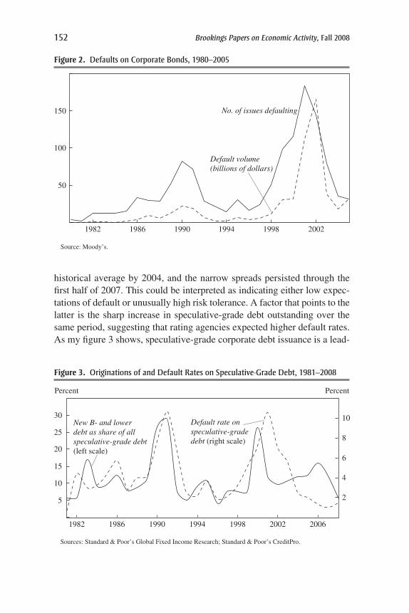
historical average by 2004, and the narrow spreads persisted through thefirst half of 2007. This could be interpreted as indicating either low expec-tations of default or unusually high risk tolerance. A factor that points to thelatter is the sharp increase in speculative-grade debt outstanding over thesame period, suggesting that rating agencies expected higher default rates.As my figure 3 shows, speculative-grade corporate debt issuance is a lead-
152 Brookings Papers on Economic Activity, Fall 2008
Figure 2. Defaults on Corporate Bonds, 1980–2005
Source: Moody’s.
1982 1986 1990 1994 1998 2002
150
100
50
No. of issues defaulting
Default volume(billions of dollars)
Figure 3. Originations of and Default Rates on Speculative-Grade Debt, 1981–2008
Sources: Standard & Poor’s Global Fixed Income Research; Standard & Poor’s CreditPro.
1982
Percent Percent
30
25
20
15
10
5
10
8
6
4
2
Default rate onspeculative-gradedebt (right scale)
New B- and lowerdebt as share of allspeculative-grade debt(left scale)
1986 1990 1994 1998 2002 2006
11472-02b_Gerardi-Comment_rev.qxd 3/6/09 12:25 PM Page 152
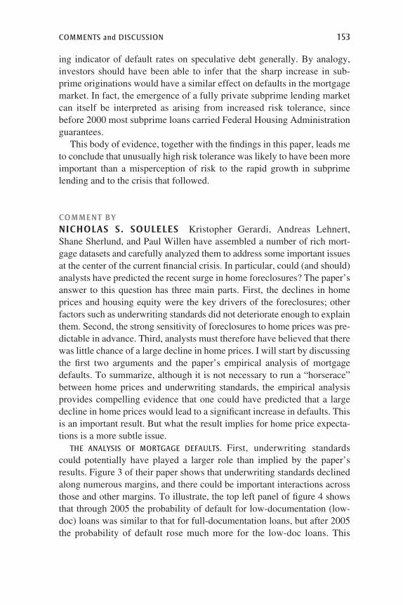
COMMENTS and DISCUSSION 153
ing indicator of default rates on speculative debt generally. By analogy,investors should have been able to infer that the sharp increase in sub-prime originations would have a similar effect on defaults in the mortgagemarket. In fact, the emergence of a fully private subprime lending marketcan itself be interpreted as arising from increased risk tolerance, sincebefore 2000 most subprime loans carried Federal Housing Administrationguarantees.
This body of evidence, together with the findings in this paper, leads meto conclude that unusually high risk tolerance was likely to have been moreimportant than a misperception of risk to the rapid growth in subprimelending and to the crisis that followed.
COMMENT BYNICHOLAS S. SOULELES Kristopher Gerardi, Andreas Lehnert,Shane Sherlund, and Paul Willen have assembled a number of rich mort-gage datasets and carefully analyzed them to address some important issuesat the center of the current financial crisis. In particular, could (and should)analysts have predicted the recent surge in home foreclosures? The paper’sanswer to this question has three main parts. First, the declines in homeprices and housing equity were the key drivers of the foreclosures; otherfactors such as underwriting standards did not deteriorate enough to explainthem. Second, the strong sensitivity of foreclosures to home prices was pre-dictable in advance. Third, analysts must therefore have believed that therewas little chance of a large decline in home prices. I will start by discussingthe first two arguments and the paper’s empirical analysis of mortgagedefaults. To summarize, although it is not necessary to run a “horserace”between home prices and underwriting standards, the empirical analysisprovides compelling evidence that one could have predicted that a largedecline in home prices would lead to a significant increase in defaults. Thisis an important result. But what the result implies for home price expecta-tions is a more subtle issue.
THE ANALYSIS OF MORTGAGE DEFAULTS. First, underwriting standardscould potentially have played a larger role than implied by the paper’sresults. Figure 3 of their paper shows that underwriting standards declinedalong numerous margins, and there could be important interactions acrossthose and other margins. To illustrate, the top left panel of figure 4 showsthat through 2005 the probability of default for low-documentation (low-doc) loans was similar to that for full-documentation loans, but after 2005the probability of default rose much more for the low-doc loans. This
11472-02b_Gerardi-Comment_rev.qxd 3/6/09 12:25 PM Page 153

154 Brookings Papers on Economic Activity, Fall 2008
suggests that some other factor that interacts with low-doc loans deterio-rated after 2005. The key question is whether this factor is (mainly) thedecrease in home prices. There are other, not mutually exclusive, possibil-ities. Suppose that before the housing boom, lenders were more likely tooffset the risk associated with low documentation by reducing risk alongother margins; for instance, by relying more on lower loan-to-value (LTV)ratios, or on higher credit scores, traditional amortization, or other positiverisk factors. This would have reduced the overall risk of low-doc loans inthe past. Conversely, there might have been more observations of badcombinations of risk factors (for example, low documentation and lowscores) in recent years. The point is that underwriting standards have manycomponents, and they can endogenously interact. In that case one cannotsimply introduce the individual components separately into an empiricalmodel. The paper recognizes this point and includes some interactionterms (“risk layering”), but only a few; these are mostly interactions withLTV and are mostly limited to the first default model, the probit modelreported in their table 5. In this sense the results provide a lower bound onthe importance of underwriting standards. It would be interesting to knowwhat greater proportion of defaults could be explained by including moreinteraction terms—indeed, as saturated a set as possible.
Further, although the paper’s datasets are rich in information about bor-rowers and their mortgages, this is still only a subset of the informationavailable to lenders for assessing their loans. For instance, the datasets lackinformation on some contract terms, such as points and fees; some applica-tion data, such as the borrowers’ financial wealth; and some credit bureaudata, such as past mortgage payment problems. Such information, which isknown by lenders, could potentially have been used to predict even moreof the increase in defaults.1
Second, it is not necessary to think of the paper’s exercise as a horseracebetween underwriting standards and home prices. To begin with, in non-linear models generally there is no unique decomposition of the impor-tance of individual explanatory variables. More substantively, if homeprices interact with underwriting standards and other factors, it is inher-ently difficult to quantify the relative importance of home prices per se.For example, a number of studies have found that low equity interacts with
1. For example, David Gross and Nicholas Souleles, “An Empirical Analysis of Per-sonal Bankruptcy and Delinquency,” Review of Financial Studies 15, no. 1 (2002): 319–47,using an administrative dataset containing all the key variables tracked by credit cardlenders, analyze the increase in consumer bankruptcy and credit card default in the late1990s.
11472-02b_Gerardi-Comment_rev.qxd 3/6/09 12:25 PM Page 154

COMMENTS and DISCUSSION 155
2. See, for example, Christopher Foote, Kristopher Gerardi, and Paul Willen, “Nega-tive Equity and Foreclosure: Theory and Evidence,” Journal of Urban Economics 64, no. 2(2008): 234–45. To illustrate, consider the polar case in which default occurs if andonly if the borrower both has negative equity and becomes unemployed. Foote and his coau-thors find that borrowers with negative equity in recent years are more likely to default thanborrowers with negative equity were in 1991 (before the growth in subprime loans), ceterisparibus. Using the ABS data in this paper, but without ending the sample in 2004, Shane M.Sherlund, “The Past, Present, and Future of Subprime Mortgages,” Staff Paper 2008-63(Washington: Federal Reserve Board of Governors, 2008), finds that borrowers with fixed-rate mortgages were less significantly sensitive to negative equity than were borrowers withadjustable-rate mortgages, ceteris paribus. Such results suggest that net equity might interactwith other factors, such as the characteristics of borrowers or their mortgage terms.
3. See, for example, Gary Gorton, “The Panic of 2007,” working paper (Yale Univer-sity, 2008).
“triggers” such as unemployment spells.2 Such triggers can also be corre-lated with underwriting standards; for example, unemployment risk couldbe correlated with a low credit score.
A larger role for declines in underwriting standards (or for other factors)can still be consistent with the overall argument of the paper, so long asthese declines were largely observable or predictable, and so long as homeprices were a predictably significant factor in generating default. If recentsubprime mortgages were even more risky, and predictably so, the argu-ment would be that this implied even more optimism about future homeprices. Pushing the argument further, many of the subprime mortgagesmight have been unviable unless the borrowers could eventually refinanceout of them, which presumes positive-enough net equity and high-enoughhome prices.3
The paper does provide compelling evidence about the predictable sig-nificance of housing equity for mortgage default. (One small quibble: Thepaper contends that analysts could have used the results for low-but-positive equity in 2000–04 to quantitatively extrapolate the effects ofnegative equity after 2004. This extrapolation depends, of course, on theassumed functional form, and analysts could not have known ex antewhich functional form would have worked well.) As for the effects ofunderwriting standards, to the extent that there were few observations inthe early data of some of the bad combinations of risk factors that becamesalient later (perhaps, for example, low documentation combined with lowcredit scores), it would have been more difficult to forecast future defaultrates with precision. In fact, the main default model applied to the ABSdata (the competing-risks model reported in table 10) could not includesome salient mortgage characteristics—not even the uninteracted effectsof nontraditional amortization, or of negative equity (that is, a nonlinear
11472-02b_Gerardi-Comment_rev.qxd 3/6/09 12:25 PM Page 155

effect for low equity, in addition to the included linear equity variables)—since there were too few observations of mortgages with those characteris-tics in the ABS data before 2004.
IMPLICATIONS FOR HOME PRICE EXPECTATIONS. Supposing it was pre-dictable that large declines in home prices would lead to large increases indefault rates, can one therefore conclude that lenders and other analystsmust not have been expecting large declines in home prices? There areagain alternative, not mutually exclusive, possibilities.
First, without complete information on the terms of the mortgage con-tracts, it remains possible that lenders thought they were offsetting some-what more of the mortgage risk than implied by the analysis. Second,lenders and investors might have been willing to tolerate some nonnegligi-ble risk of a large decline in home prices, if their risk aversion was lowenough and they considered alternative outcomes (such as a period of stag-nant home prices) sufficiently likely. Third, insofar as agency problemswere important, some lenders might have thought that they would not fullybear the costs of the increased defaults, even if they could have predictedthem.4 To investigate this possibility, one would ideally like to distinguishthe information set of the mortgage originators from the information setsof investors and other agents, which presumably are subsets of the former,to see whether the additional information available to the originatorswould have predicted significantly more of the defaults.
Finally, even if analysts should have been able to predict much of theincrease in mortgage defaults, it would have been more difficult to forecasttheir spillover onto the rest of the financial system and the extent of theresulting crisis, and moreover to forecast how the crisis in turn would spillback into the mortgage market, further increasing defaults through evenlower home prices and other mechanisms (such as higher unemployment).
Although the paper’s competing-risks models explain much of theincrease in defaults, in the end they still generally underpredict them, espe-cially for the 2005 vintage of mortgages. The paper suggests that this couldreflect the fact that the 2005 vintage was more exposed than the 2004 vin-tage to home price declines. However, the competing-risks models are
156 Brookings Papers on Economic Activity, Fall 2008
4. On this topic, see, for example, Adam Ashcraft and Til Schuermann, “Understandingthe Securitization of Subprime Mortgage Credit,” Staff Report 318 (Federal Reserve Bankof New York, 2008); Charles Calomiris, “The Subprime Turmoil: What’s Old, What’s New,and What’s Next,” working paper (Columbia University, 2008); Benjamin Keys and others,“Securitization and Screening: Evidence from Subprime Mortgage Backed Securities,”working paper (University of Michigan, 2008); and Atif Mian and Amir Sufi, “The Conse-quences of Mortgage Credit Expansion: Evidence from the 2007 Mortgage Default Crisis,”working paper (University of Chicago, 2008).
11472-02b_Gerardi-Comment_rev.qxd 3/6/09 12:25 PM Page 156

COMMENTS and DISCUSSION 157
supposed to control for the effects of lower home prices through lowerhousing equity (and for the resulting decline in the borrower’s ability torefinance the mortgage or sell the home instead of defaulting). Howmuch larger a share of the observed defaults could be explained throughimproved measurement and modeling of housing equity remains an openquestion. Perhaps other relevant risk factors are still missing from themodel, or perhaps the increase in defaults was to some degree inherentlydifficult to predict in advance, even given the path of home prices.Nonetheless, the paper has made a valuable contribution in showing thathome prices were in any case a predictably significant contributor to thedefaults.
GENERAL DISCUSSION Jan Hatzius remarked that the idea that peo-ple incorrectly guessed the direction of home prices but not the relation-ship between home prices and defaults was consistent with his impressionfrom discussions he had had with market analysts over the past few years.Most refused to believe, despite a history of large regional declines inhome prices, and of nationwide declines in other countries, that homeprices in the United States could decline in nominal terms. This denial, hebelieved, was the essential problem that led to the crisis.
Karl Case stressed the importance of examining the data at the regionallevel. What was happening in Florida, Nevada, and Arizona, for example,was very different from what was occurring in the Midwest and the North-east. California’s situation was particularly notable since that state accountsfor 25 percent of the nation’s housing value and experienced a steep declinein prices. He added that the laws relevant to housing differ in importantways from state to state, and that markets clear at different rates in differ-ent areas.
Austan Goolsbee offered an airline analogy to illustrate how the crisisarose largely from the interaction of declining home prices and deterio-rating lending standards, with the latter playing the lead role. To enablepeople with bad credit to buy homes, the financial markets had createdsubprime mortgages and other products that translated home price appreci-ation into broader home ownership. Just as flying on a budget airline is fineuntil something goes wrong, so these subprime mortgages were fine untilprices started to fall. Goolsbee added that the securitization of those mort-gages was much more complicated than what the paper portrayed, and thatlending standards deteriorated not only through the relaxation of lendingcriteria but also through outright fraud: people were allowed to lie about
11472-02b_Gerardi-Comment_rev.qxd 3/6/09 12:25 PM Page 157

the owner-occupier status of the home they purchased. This mattersbecause people are more likely to walk away from a second home thanfrom a primary residence as soon as they fall into negative equity. Lendersshould have assumed that the market would go bad at some point andpriced their loans accordingly.
Frederic Mishkin noted that the adjustable subprime contracts inher-ently assumed a rise in asset prices, because otherwise the loans would notcontinue to be serviced when the interest rate was reset. Lenders assumedthat prices would continue to rise, turning subprime borrowers into primeborrowers, who could then refinance the loan on better terms. He indicatedthat loans made with the expectation that they would be refinanced mayhave been prompted by underlying principal-agent issues.
Robert Hall mentioned the work of John Campbell and Robert Shillershowing that overvaluation in a stock market can be detected by looking atthe price-dividend ratio: the higher the ratio, the higher the likelihood of aprice decline. He suggested incorporating this type of analysis into thepaper by looking at price-rent or price-income ratios, noting that theirunprecedentedly high levels in the mid-2000s signaled a high probabilityof future decline.
Martin Baily directed the Panel’s attention to the prices of ABXsecurities—the collateralized debt obligations built on the mortgage-backed securities—and to delinquency rates, which, he argued, revealed alikely change in underwriting standards in the years before the crisis. ABXsecurities declined significantly in price between the first and the secondquarters of 2006, too short an interval to be explained by a drastic changein the underlying mortgages. Delinquency rates, in contrast, increasedsharply in the fourth quarter of 2005 and continued to rise in subsequentquarters. The dissimilarity between these two data series seems to indicatea change in something other than housing prices, such as underwritingstandards.
Charles Schultze summarized the paper as saying that analysts didunderstand the nonlinear dependence of foreclosures on changes in homeprices but were shocked by the idea that home prices would fall as much asthey did. He attributed the unusual size of the price drop to the fact thatthere had not been an upward movement in home prices this large in theprevious forty years. He blamed the incentive structure facing the man-agers and employees of financial firms: one’s approach to risk manage-ment changes if one can expect bonuses for four or five years on the upsideand only miss one or two on the inevitable downside. He cited a UBSreport written after the bank lost the first $19 billion of $42 billion in even-
158 Brookings Papers on Economic Activity, Fall 2008
11472-02b_Gerardi-Comment_rev.qxd 3/6/09 12:25 PM Page 158

COMMENTS and DISCUSSION 159
tual losses, in which the downplaying of risk management is noted. Inaddition, the lack of attention to risk evaluation by investors generated asurge in demand for subprime mortgage-backed securities that put pressureon mortgage originators for a substantial erosion of underwriting standards.
Lawrence Summers noted the long tradition of financial messes madebecause people observed that over a long period the strategy of writingout-of-the-money puts had proved consistently profitable, and so contin-ued the strategy until inevitably a problem occurred. He seconded Gools-bee’s comment on the interaction of factors deepening the crisis and askedthe authors to try to tease out these different factors. He also suggested thatthe authors examine the strategies pursued by major builders, the stockprices of those builders, and the implied volatility in puts on their stocks,since builders are essentially betting their franchises on the housing busi-ness remaining strong. He guessed that such an examination of these fac-tors would show that the builders shared in the euphoria of rising homeprices yet did not share in the ignorance—an idea at odds with Schultze’semphasis on Wall Street’s compensation structures.
Bradford DeLong came to the defense of those who had bought homes inCalifornia, Florida, and Boston, arguing that long-term interest rates willeventually decline, leading to an increase in home price–rent ratios. Also,rising population in the United States will eventually lead to increased con-gestion, so land will essentially become a Hotelling good with prices risingover time.
Richard Cooper remarked that one should not limit one’s analysis ofhome price–income ratios to a period of worldwide decline in real long-term interest rates, because housing is a long-term asset. He also pointed outthat, at least in the United States, the income elasticity of demand for hous-ing is significantly greater than one, so that rising incomes would eventuallylead to an increase in home price–income ratios. But it would be too sim-plistic to make an evaluation from this ratio alone.
11472-02b_Gerardi-Comment_rev.qxd 3/6/09 12:25 PM Page 159

11472-02b_Gerardi-Comment_rev.qxd 3/6/09 12:25 PM Page 160