Inferenc.docx

Making Inferences About Parameters

Parametric statistical inference may take the form of:

1. Estimation: on the basis of sample data we estimate the value of some parameter of the population from which the sample was randomly drawn.

2. Hypothesis Testing: We test the null hypothesis that a specified parameter (I shall use to stand for the parameter being estimated) of the population has a specified value.

One must know the sampling distribution of the estimator (the statistic used to estimate - I

shall use to stand for the statistic used to estimate ) to make full use of the estimator. The sampling distribution of a statistic is the distribution that would be obtained if you repeatedly drew

samples of a specified size from a specified population and computed on each sample. In other words, it is the probability distribution of a statistic.

Desirable Properties of Estimators Include:

1. Unbiasedness: is an unbiased estimator of if its expected value equals the value of the

parameter being estimated, that is, if the mean of its sampling distribution is . The sample mean and sample variance are unbiased estimators of the population mean and population variance (but sample standard deviation is not an unbiased estimator of population standard deviation).

For a discrete variable X, E(X), the expected value of X, is: ii XPXE )( . For example, if

50% of the bills in a pot are one-dollar bills, 30% are two-dollar bills, 10% are five-dollar bills, 5% are ten-dollar bills, 3% are twenty-dollar bills, and 2% are fifty-dollar bills, the expected value for the value of what you get when you randomly select one bill is .5(1) + .3(2) + .1(5) + .05(10) + .03(20) + .02(50) = $3.70. For a continuous variable the basic idea of an expected value is the same as for a discrete variable, but a little calculus is necessary to “sum” up the infinite number of products of Pi (actually, probability “density”) and Xi.

Please note that the sample mean is an unbiased estimator of the population mean, and the

sample variance, s2, SS / (N - 1), is an unbiased estimator of the population variance, 2. If we computed the estimator, s2, with (N) rather than (N-1) in the denominator then the estimator would be

biased. SS is the sum of the squared deviations of scores from their mean, 2)( YMY .

The sample standard deviation is not, however, an unbiased estimator of the population standard deviation (it is the least biased estimator available to us). Consider a hypothetical sampling distribution for the sample variance where half of the samples have s2 = 2 and half have s2 = 4. Since the sample variance is totally unbiased, the population variance must be the expected value of

the sample variances, .5(2) + .5(4) = 3, and the population standard deviation must be 732.13 .

Now consider the standard deviations. 707.145.25.)( sE . Since the expected value of the

sample standard deviations, 1.707, is not equal to the true value of the estimated parameter, the sample standard deviation is not unbiased. It is, however, less biased than it would be were we to use (N) rather than (N-1) in the denominator.

2. Relative Efficiency: an efficient estimator is one whose sampling distribution has little variability. For an efficient estimator, the variance (and thus the standard deviation too) of the sampling distribution is small. The standard deviation of a sampling distribution is known as its standard error. With an efficient estimator the statistics in the sampling distribution will not differ

Copyright 2014, Karl L. Wuensch - All rights reserved.

2 much from each other, and accordingly when you randomly draw one sample your estimate is likely to have less error than it would if you had employed a less efficient estimator.

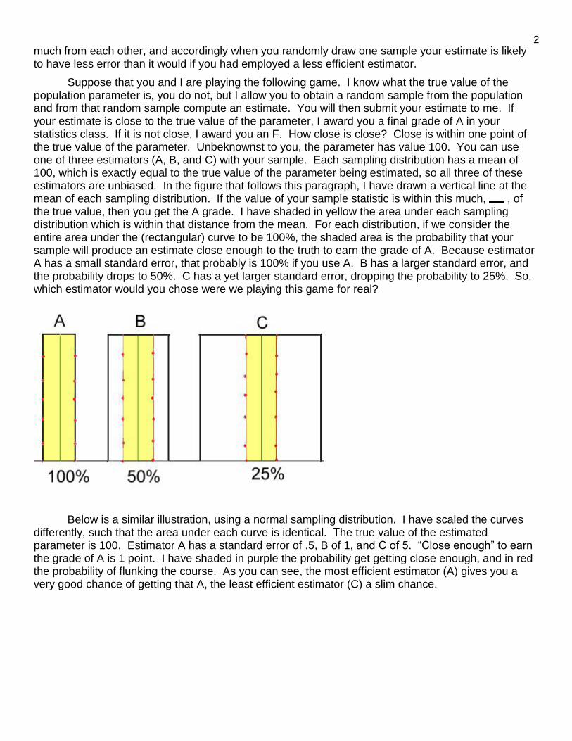
Suppose that you and I are playing the following game. I know what the true value of the population parameter is, you do not, but I allow you to obtain a random sample from the population and from that random sample compute an estimate. You will then submit your estimate to me. If your estimate is close to the true value of the parameter, I award you a final grade of A in your statistics class. If it is not close, I award you an F. How close is close? Close is within one point of the true value of the parameter. Unbeknownst to you, the parameter has value 100. You can use one of three estimators (A, B, and C) with your sample. Each sampling distribution has a mean of 100, which is exactly equal to the true value of the parameter being estimated, so all three of these estimators are unbiased. In the figure that follows this paragraph, I have drawn a vertical line at the mean of each sampling distribution. If the value of your sample statistic is within this much, , of the true value, then you get the A grade. I have shaded in yellow the area under each sampling distribution which is within that distance from the mean. For each distribution, if we consider the entire area under the (rectangular) curve to be 100%, the shaded area is the probability that your sample will produce an estimate close enough to the truth to earn the grade of A. Because estimator A has a small standard error, that probably is 100% if you use A. B has a larger standard error, and the probability drops to 50%. C has a yet larger standard error, dropping the probability to 25%. So, which estimator would you chose were we playing this game for real?

Below is a similar illustration, using a normal sampling distribution. I have scaled the curves differently, such that the area under each curve is identical. The true value of the estimated parameter is 100. Estimator A has a standard error of .5, B of 1, and C of 5. “Close enough” to earn the grade of A is 1 point. I have shaded in purple the probability get getting close enough, and in red the probability of flunking the course. As you can see, the most efficient estimator (A) gives you a very good chance of getting that A, the least efficient estimator (C) a slim chance.

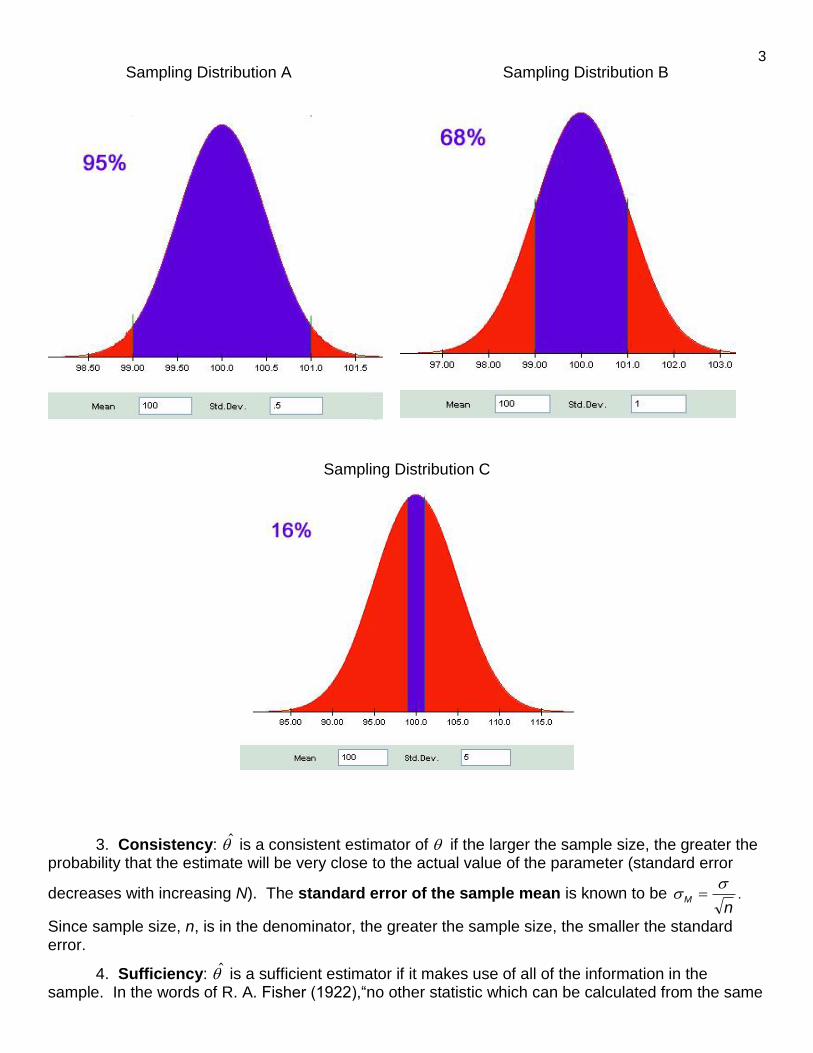
3 Sampling Distribution A Sampling Distribution B

Sampling Distribution C

3. Consistency: is a consistent estimator of if the larger the sample size, the greater the probability that the estimate will be very close to the actual value of the parameter (standard error

decreases with increasing N). The standard error of the sample mean is known to be n

M

.

Since sample size, n, is in the denominator, the greater the sample size, the smaller the standard error.

4. Sufficiency: is a sufficient estimator if it makes use of all of the information in the sample. In the words of R. A. Fisher (1922),“no other statistic which can be calculated from the same

4 sample provides any additional information as to the value of the parameter.” The sample variance, for example, is more sufficient than the sample range, since the former uses all the scores in the sample, the latter only two.

5. Resistance: is a resistant estimator to the extent that it is not influenced by the presence of outliers. For example, the median resists the influence of outliers more than does the mean.

We will generally prefer sufficient, consistent, unbiased, resistant, efficient estimators. In some cases the most efficient estimator may be more biased than another. If we wanted to enhance the probability of being very close to the parameter’s actual value on a single estimate we might choose the efficient, biased estimator over a less efficient but unbiased estimator.

After a quiz on which she was asked to list the properties which are considered desirable in estimators, graduate student Lisa Sadler created the following acronym: CURSE (consistency, unbiasedness, resistance, sufficiency, efficiency).

Types of Estimation

1. Point Estimation: estimate a single value for which is, we hope, probably close to the

true value of .

2. Interval Estimation: find an interval, the confidence interval, which has a given

probability (the confidence coefficient) of including the true value of .

a. For estimators with normally distributed sampling distributions, a confidence interval (CI)

with a confidence coefficient of CC = (1 - ) is:

ˆˆˆˆ zz

Alpha () is the probability that the CI will not include the true value of . Z is the number of standard deviations one must go below and above the mean of a normal distribution to mark off the

middle CC proportion of the area under the curve, excluding the most extreme proportion of the

scores, / 2 in each tail.

is the standard error, the standard deviation of the sampling

distribution of .

b. A 95% CI will extend from

ˆˆ 96.1ˆ96.1ˆ if the sampling distribution is normal.

We would be 95% confident that our estimate-interval included the true value of the estimated

parameter (if we drew a very large number of samples 95% of them would have intervals which

would in fact include the true value of ). If CC = .95, a fair bet would be placing 19:1 odds in favor

of CI containing .

c. The value of Z will be 2.58 for a 99% CI, 2.33 for a 98% CI, 1.645 for a 90% CI, 1.00 for a 68% CI, 2/3 for a 50% CI, other values obtainable from the normal curve table.

d. Consider this very simple case. We know that a population of IQ scores is normally

distributed and has a of 15. We have randomly sampled one score and it is 110. When N = 1, the

standard error of the mean, M = population . Thus, a 95% CI would be 110 1.96(15). That is,

we are 95% confident that the is between 80.6 and 139.4.

Hypothesis Testing

A second type of inferential statistics is hypothesis testing. For parametric hypothesis testing

one first states a null hypothesis (H). The H specifies that some parameter has a particular value or has a value in a specified range of values. For nondirectional hypotheses, a single value is

stated. For example, = 100. For directional hypotheses a value of less than or equal to (or

greater than or equal to) some specified value is hypothesized. For example, 100.

5

The alternative hypotheses (H1) is the antithetical complement of the H. If the H is =

100, the H1 is 100. If H is 100, H1 is > 100. H: 100 implies H1: < 100. The H and the H1 are mutually exclusive and exhaustive: one, but not both, must be true.

Notice that the null hypothesis always includes an equals sign (≤, =, or ≥) and the alternative hypothesis never does (does include <, ≠, or >).

Equality and inequality signs.

A < B: A is less than B.

A = ≤ B: A is less than or equal to B.

A = B: A is equal to B.

A ≥ B: A is greater than or equal to B.

A > B: A is greater than B.

A ≠ B: A is not equal to B.

Very often the behavioral scientist wants to reject the H and assert the H1. For example, e

may think e’s students are brighter than normal, so e sets up the H that 100 for IQ, hoping to

show that H is not reasonable, thus asserting the H1 that > 100. Sometimes, however, one wishes

not to reject a H. For example, I may have a mathematical model that predicts that the average

amount of rainfall on an April day in Soggy City is 9.5 mm, and if my data lead me to reject that H, then I have shown my model to be inadequate and in need of revision.

The H is tested by gathering data that are relevant to the hypothesis and determining how

well the data fit the H. If the fit is poor, we reject the H and assert the H1. We measure how well

the data fit the H with an exact significance level, p, which is the probability of obtaining a

sample as or more discrepant with the H than is that which we did obtain, assuming that the

H is true. The higher this p, the better the fit between the data and the H. If this p is low we have

cast doubt upon the H. If p is very low, we reject the H. How low is very low? Very low is usually

.05 -- the criterion used to reject the H is p .05 for behavioral scientists, by convention, but I opine that an individual may set e’s own criterion by considering the implications thereof, such as the

likelihood of falsely rejecting a true H (an error which will be more likely if one uses a higher

criterion, such as p .10).

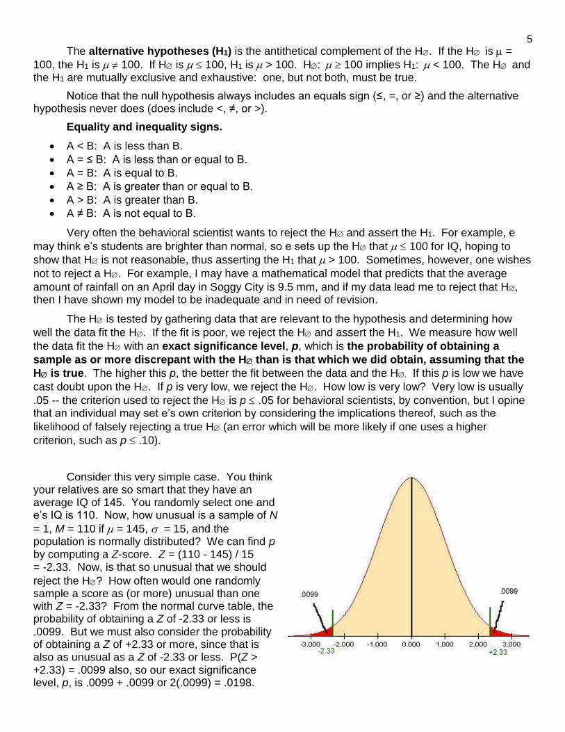
Consider this very simple case. You think your relatives are so smart that they have an average IQ of 145. You randomly select one and e’s IQ is 110. Now, how unusual is a sample of N

= 1, M = 110 if = 145, = 15, and the population is normally distributed? We can find p by computing a Z-score. Z = (110 - 145) / 15 = -2.33. Now, is that so unusual that we should

reject the H? How often would one randomly sample a score as (or more) unusual than one with Z = -2.33? From the normal curve table, the probability of obtaining a Z of -2.33 or less is .0099. But we must also consider the probability of obtaining a Z of +2.33 or more, since that is also as unusual as a Z of -2.33 or less. P(Z > +2.33) = .0099 also, so our exact significance level, p, is .0099 + .0099 or 2(.0099) = .0198.

6

What does p = .0198 mean? It means that were we repeatedly to sample scores from a

normal population with = 145, =15, a little fewer than 2% of them would be as unusual (as far

away from the of 145) or more unusual than the sample score we obtained, assuming the H is

true. In other words, either we just happened to select an unusual score, or the H is not really true.

So what do we conclude? Is the H false or was our sample just unusual? Here we need a

decision rule: If p is less than or equal to an a priori criterion, we reject the H; otherwise we

retain it. The most often used a priori criterion is .05. Since p = .0198 < .05, we reject the H and

conclude that is not equal to 145.

Statistical significance. When we reject a null hypothesis, we describe our result as “significant.” In this context, “significant” does not necessary imply “important” or “large” or “of great interest.” It simply means that we have good evidence against the null hypothesis – that is, the obtained sample is very different from what we would expect were the null hypothesis true. In behavioral research, the null hypothesis usually boils down to a “nil” hypothesis – the hypothesis that the correlation between two things or two sets of things is absolutely zero – that is, the two things are absolutely independent of each other, not related to each other. When we reject the null hypothesis, we infer that the two things are related to each other. Then we make a strong statement about the direction of that relationship. For example, if my research revealed that taking a new antihistamine significantly increased patients’ reactions times, I would be confident that taking the drug is positively correlated with reaction times. If my result was not significant, I might still suspect that it has some undetected effect, but I would not be confident about the direction of the effect – it could be positive, it could be negative, it conceivably could even be nil.

Type I Error. What are the chances that we made a mistake, that the H was true and we just happened to get an unusual sample? Alpha is the probability of making a Type I Error, the

conditional probability of rejecting the H given that the H is true. By setting the a priori criterion to

.05, we assured that would be .05 or less. Our exact is p, .0198 for this sample.

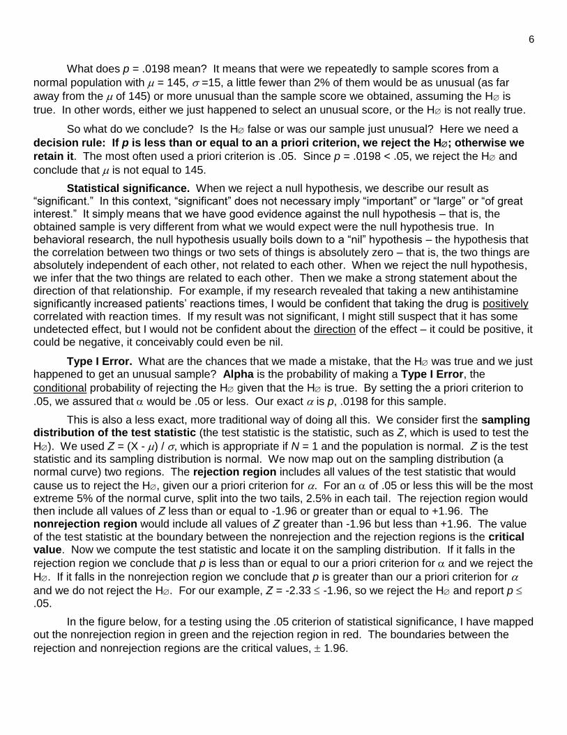
This is also a less exact, more traditional way of doing all this. We consider first the sampling distribution of the test statistic (the test statistic is the statistic, such as Z, which is used to test the

H). We used Z = (X - ) / , which is appropriate if N = 1 and the population is normal. Z is the test statistic and its sampling distribution is normal. We now map out on the sampling distribution (a normal curve) two regions. The rejection region includes all values of the test statistic that would

cause us to reject the H, given our a priori criterion for . For an of .05 or less this will be the most extreme 5% of the normal curve, split into the two tails, 2.5% in each tail. The rejection region would then include all values of Z less than or equal to -1.96 or greater than or equal to +1.96. The nonrejection region would include all values of Z greater than -1.96 but less than +1.96. The value of the test statistic at the boundary between the nonrejection and the rejection regions is the critical value. Now we compute the test statistic and locate it on the sampling distribution. If it falls in the

rejection region we conclude that p is less than or equal to our a priori criterion for and we reject the

H. If it falls in the nonrejection region we conclude that p is greater than our a priori criterion for

and we do not reject the H. For our example, Z = -2.33 -1.96, so we reject the H and report p .05.

In the figure below, for a testing using the .05 criterion of statistical significance, I have mapped out the nonrejection region in green and the rejection region in red. The boundaries between the

rejection and nonrejection regions are the critical values, 1.96.

7

I prefer that you report an exact p rather than just saying that p .05 or p > .05. Suppose that a reader of your research report thinks the a priori criterion should have been .01, not .05. If you

simply say p .05, e doesn’t know whether to reject or retain the H with set at .01 or less. If you report p = .0198, e can make such decisions. Imagine that our p came out to be .057. Although we

would not reject the H, it might be misleading to simply report “p > .05, H not rejected.” Many

readers might misinterpret this to mean that your data showed the H to be true. In fact, p = .057 is

pretty strong evidence against the H, just not strong enough to warrant a rejection with an a priori

criterion of .05 or less. Were the H the defendant in your statistical court of law, you would find it not guilty, which is not the same as innocent. The data cast considerable doubt upon the veracity of the

H, but not “beyond a reasonable doubt,” where “beyond a reasonable doubt” means p is less than or

equal to the a priori criterion for .

Now, were p = .95, I might encourage you not only to fail to reject the H, but to assert its truth or near truth. But using the traditional method, one would simply report p > .05 and readers could not simply discriminate between the case when p = .057 and that when p = .95.

Please notice that we could have decided whether or not to reject the H on the basis of the

95% CI we constructed earlier. Since our CC was 95% we were using an of (1 - CC) = .05. Our CI

for extended from 80.6 to 139.4, which does not include the hypothesized value of 145. Since we

are 95% confident that the true value of is between 80.6 and 139.4, we can also be at least 95%

confident (5% ) that is not 145 (or any other value less than 80.6 or more than 139.4) and reject

the H. If our CI included the value of hypothesized in the H, for example, if our H were = 100,

then we could not reject the H.

The CI approach does not give you a p value with which quickly to assess the likelihood that a type I error was made. It does, however, give you a CI, which hypothesis testing does not. I suggest

that you give your readers both p and a (1-) CI as well as your decision regarding rejection or

nonrejection of the H.

You now know that is the probability of rejecting a H given that it is really true. Although

traditionally set at .05, I think one should set e’s criterion for at whatever level e thinks reasonable,

8 considering the danger involved in making a type two error. A Type II error is not rejecting a false

H, and Beta ( ) is the conditional probability of not rejecting the H given that it is really false. The

lower one sets the criterion for , the larger will be, ceteris paribus, so one should not just set very low and think e has no chance of making any errors.

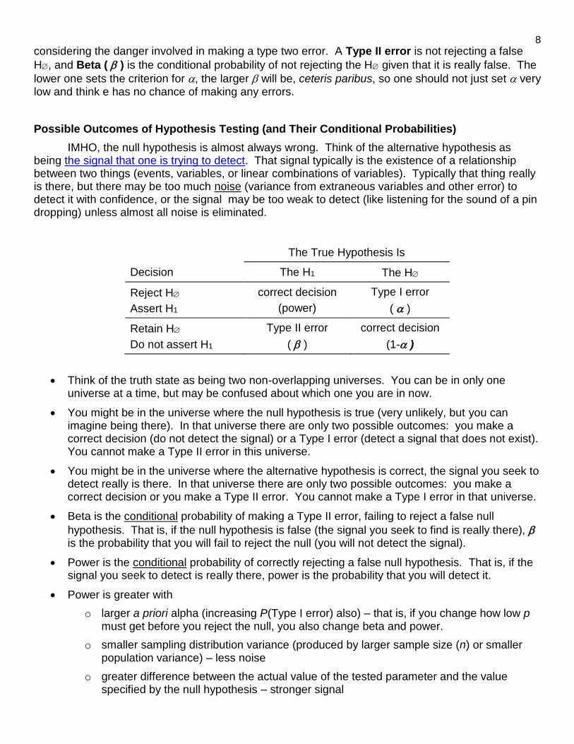
Possible Outcomes of Hypothesis Testing (and Their Conditional Probabilities)

IMHO, the null hypothesis is almost always wrong. Think of the alternative hypothesis as being the signal that one is trying to detect. That signal typically is the existence of a relationship between two things (events, variables, or linear combinations of variables). Typically that thing really is there, but there may be too much noise (variance from extraneous variables and other error) to detect it with confidence, or the signal may be too weak to detect (like listening for the sound of a pin dropping) unless almost all noise is eliminated.

The True Hypothesis Is

Decision The H1 The H

Reject H

Assert H1

correct decision

(power)

Type I error

( )

Retain H

Do not assert H1

Type II error

( )

correct decision

(1- )

Think of the truth state as being two non-overlapping universes. You can be in only one universe at a time, but may be confused about which one you are in now.

You might be in the universe where the null hypothesis is true (very unlikely, but you can imagine being there). In that universe there are only two possible outcomes: you make a correct decision (do not detect the signal) or a Type I error (detect a signal that does not exist). You cannot make a Type II error in this universe.

You might be in the universe where the alternative hypothesis is correct, the signal you seek to detect really is there. In that universe there are only two possible outcomes: you make a correct decision or you make a Type II error. You cannot make a Type I error in that universe.

Beta is the conditional probability of making a Type II error, failing to reject a false null

hypothesis. That is, if the null hypothesis is false (the signal you seek to find is really there), is the probability that you will fail to reject the null (you will not detect the signal).

Power is the conditional probability of correctly rejecting a false null hypothesis. That is, if the signal you seek to detect is really there, power is the probability that you will detect it.

Power is greater with

o larger a priori alpha (increasing P(Type I error) also) – that is, if you change how low p must get before you reject the null, you also change beta and power.

o smaller sampling distribution variance (produced by larger sample size (n) or smaller population variance) – less noise

o greater difference between the actual value of the tested parameter and the value specified by the null hypothesis – stronger signal

9 o one-tailed tests (if the predicted direction (specified in the alternative hypothesis) is

correct) – paying attention to the likely source of the signal

o some types of tests (t test) than others (sign test) – like a better sensory system

o some research designs (matched subjects) under some conditions (matching variable correlated with DV)

Suppose you are setting out to test a hypothesis. You want to know the unconditional probability of making an error (Type I or Type II). That probability depends, in large part, on the probability of being in the one or the other universe, that is, on the probability of the null

hypothesis being true. This unconditional error probability is equal to P(H true) + P(H1 true).

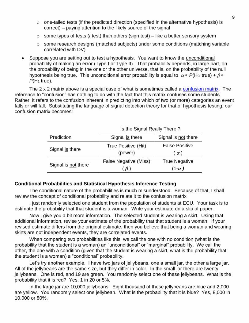
The 2 x 2 matrix above is a special case of what is sometimes called a confusion matrix. The reference to “confusion” has nothing to do with the fact that this matrix confuses some students. Rather, it refers to the confusion inherent in predicting into which of two (or more) categories an event falls or will fall. Substituting the language of signal detection theory for that of hypothesis testing, our confusion matrix becomes:

Is the Signal Really There ?

Prediction Signal is there Signal is not there

Signal is there True Positive (Hit)

(power)

False Positive

( )

Signal is not there False Negative (Miss)

( )

True Negative

(1- )

Conditional Probabilities and Statistical Hypothesis Inference Testing

The conditional nature of the probabilities is much misunderstood. Because of that, I shall review the concept of conditional probability and relate it to the confusion matrix

I just randomly selected one student from the population of students at ECU. Your task is to estimate the probability that that student is a woman. Write your estimate on a slip of paper.

Now I give you a bit more information. The selected student is wearing a skirt. Using that additional information, revise your estimate of the probability that that student is a woman. If your revised estimate differs from the original estimate, then you believe that being a woman and wearing skirts are not independent events, they are correlated events.

When comparing two probabilities like this, we call the one with no condition (what is the probability that the student is a woman) an “unconditional” or “marginal” probability. We call the other, the one with a condition (given that the student is wearing a skirt, what is the probability that the student is a woman) a “conditional” probability.

Let’s try another example. I have two jars of jellybeans, one a small jar, the other a large jar. All of the jellybeans are the same size, but they differ in color. In the small jar there are twenty jellybeans. One is red, and 19 are green. You randomly select one of these jellybeans. What is the probability that it is red? Yes, 1 in 20 or 5%.

In the large jar are 10,000 jellybeans. Eight thousand of these jellybeans are blue and 2,000 are yellow. You randomly select one jellybean. What is the probability that it is blue? Yes, 8,000 in 10,000 or 80%.

10 Good so far? OK, now a transition to the probabilities associated with the so-called “confusion matrix” often discussed in the context of hypothesis testing and signal detection. The jellybeans in the small jar represent the decisions made by psychologists testing absolutely true null hypotheses, using the traditional 5% criterion of statistical significance. Five percent of the time they will draw a red jellybean, which represents an error (Type I, Alpha = 5%), and 95% of the time they will draw a green jellybean, which represents a correct decision. Note that these are conditional probabilities. The condition is that the null hypothesis is absolutely true (you drew from the small jar).

OK, now switch jars. In the large jar the jellybeans represent the decisions made by psychologists testing null hypothesis that are wrong, and with a good chance of detecting that they are wrong (good power). Twenty percent of the time they will draw a yellow jellybean, which represents an error (Type II, Beta = 20%), and 80% of the time they will draw a blue jellybean, which represents a correct decision (power = 80%). Note that these too are conditional probabilities. The condition is that the null hypothesis is wrong (you drew from the big jar).

So, why did I use different sized jars. I used the small jar to represent research in which the null hypothesis is absolutely wrong. I made it small because it highly unlikely that the null hypothesis tested by a psychologist is going to be correct. Our null hypothesis almost always are that the correlation between two variables (or two sets of variables) is zero. We almost always have good reason, a priori, to think that null hypothesis is wrong. Most often the null is going to be wrong, thus the other jar is much larger.

OK, now dump both jars into a vat and mix the jellybeans well. Randomly draw one jellybean. What is the probability that it is red (representing a Type I error)? You have 10,020 jellybeans, only one of which is red, so the probability of a Type I error is 1 in 10,020 or 0.001%. Note that this is not a conditional probability. You don’t know whether the null hypothesis is correct or not. This is the overall, marginal, or unconditional probability of a Type I error.

Regretfully, many psychologists do not understand the conditional nature of alpha. Many suffer from the delusion that use of the 5% criterion of statistical significance will result in five percent of research tests resulting in Type I errors. As the analysis above shows, this is clearly not the case.

For more on this topic, see Frequency of Type I Errors in Professional Journals.

Sample Size Does NOT Affect the Probability of a Type I Error

The delusion that it does was identified by Rosenthal and Gaito in 1963. This delusion has persisted across several decades, despite many efforts to dispel it. The effect of sample size is incorporated into the p value that is used to determine whether or not the researcher has data sufficiently discrepant with the null hypothesis to reject it. Sample size does affect the probability of a Type II error. If the effect (the magnitude of the difference between the null hypothesis and the truth) is small, you will need a large sample to detect it. If the effect is large, you will be able to detect it even with a small sample size. It is easier to find big things than small things. Accordingly, finding a "significant" effect with a small sample size is actually very impressive, as that is likely only if the effect is large. Finding a sample size with a large sample could result only from the increased power associated with large sample sizes. Frankly, IMHO, the "significance" of an effect is a helluva lot less important than is estimation of the size of that effect. This is a problem associated with the uncritical acceptance of NHST (Null Hypothesis Statistical Testing), amusing described by Cohen (1994) as SHIT (Statistical Hypothesis Inference Testing).

Relative Seriousness of Type I and Type II Errors

Imagine that you are testing an experimental drug that is supposed to reduce blood pressure, but is suspected of inducing cancer. You administer the drug to 10,000 rodents. Since you know that

the tumor rate in these rodents is normally 10%, your H is that the tumor rate in drug-treated rodents

is 10% or less. That is, the H is that the drug is safe, it does not increase cancer rate. The H1 is that

11 the drug does induce cancer, that the tumor rate in treated rodents is greater than 10%. [Note that

the H always includes an “=,” but the H1 never does.] A Type II error (failing to reject the H of safety when the drug really does cause cancer) seems more serious than a Type I error (rejecting the

H of safety when the drug is actually safe) here (assuming that there are other safe treatments for hypertensive folks so we don’t need to weigh risk of cancer versus risk of hypertension), so we would

not want to place so low that was unacceptably large. If that H (drug is safe) is false, we want to be sure we reject it. That is, we want to have a powerful test, one with a high probability of detecting

false H hypotheses. Power is the conditional probability of rejecting a H given that it is false, and

Power = 1 - .

Now suppose we are testing the drug’s effect on blood pressure. The H is that the mean decrease in blood pressure after giving the drug (pre-treatment BP minus post-treatment BP) is less than or equal to zero (the drug does not reduce BP). The H1 is that the mean decrease is greater than zero (the drug does reduce BP). Now a Type I error (claiming the drug reduces BP when it actually does not) is clearly more dangerous than a type II error (not finding the drug effective when indeed it is), again assuming that there are other effective treatments and ignoring things like your boss’ threat to fire you if you don’t produce results that support e’s desire to market the drug. You

would want to set the criterion for relatively low here.

Directional and Nondirectional Hypotheses

Notice that in these last two examples the H was stated as “Parameter some value.” When

that is the case or when the H states “ Parameter some value,” directional hypotheses are being

tested. When the H is “Parameter = some value” nondirectional hypotheses are being used. With nondirectional hypotheses and a normal sampling distribution there are rejection regions in both tails of the sampling distribution, so this sort of test is often called a two-tailed test. When computing the p for such a two-tailed test one must double the one-tailed probability obtained from the normal curve

table prior to comparing it to the criterion for . We doubled .0099 to .0198 before comparing to .05 with our IQ example.

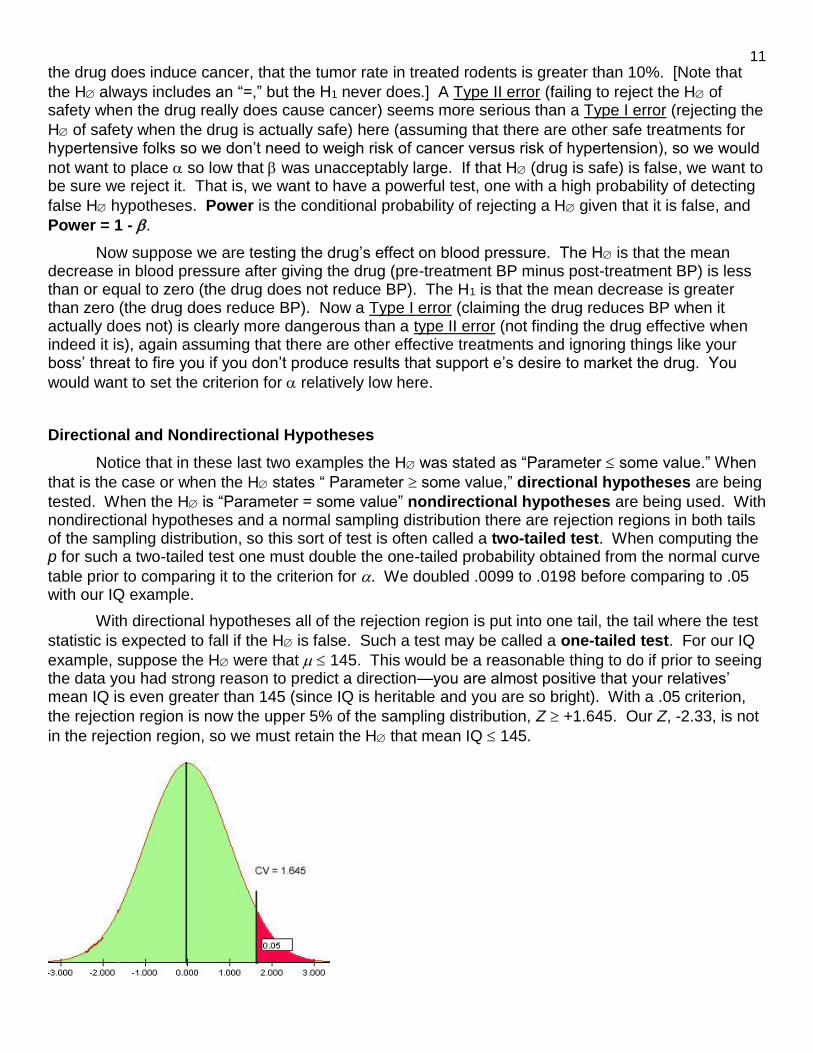
With directional hypotheses all of the rejection region is put into one tail, the tail where the test

statistic is expected to fall if the H is false. Such a test may be called a one-tailed test. For our IQ

example, suppose the H were that 145. This would be a reasonable thing to do if prior to seeing the data you had strong reason to predict a direction—you are almost positive that your relatives’ mean IQ is even greater than 145 (since IQ is heritable and you are so bright). With a .05 criterion,

the rejection region is now the upper 5% of the sampling distribution, Z +1.645. Our Z, -2.33, is not

in the rejection region, so we must retain the H that mean IQ 145.

12

When the sample results come out in a direction opposite that predicted in the H1, the H

can never be rejected. For our current example the H1 is that > 145, but X was only 110, which is less than 145. In such a case p will be the area under the sampling distribution from the value of the test statistic to the more distant tail. Using the “larger portion” column of the normal curve table, P(Z

< -2.33) = .9901 > .05, we retain the H. In fact, with p close to 1, the H looks very good.

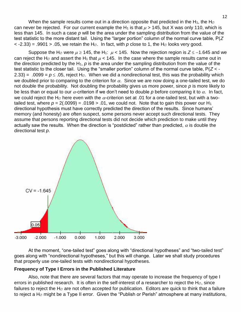
Suppose the H were 145, the H1: < 145. Now the rejection region is Z 1.645 and we

can reject the H and assert the H1 that < 145. In the case where the sample results came out in the direction predicted by the H1, p is the area under the sampling distribution from the value of the test statistic to the closer tail. Using the “smaller portion” column of the normal curve table, P(Z < -

2.33) = .0099 = p .05, reject H. When we did a nondirectional test, this was the probability which

we doubled prior to comparing to the criterion for . Since we are now doing a one-tailed test, we do not double the probability. Not doubling the probability gives us more power, since p is more likely to

be less than or equal to our -criterion if we don’t need to double p before comparing it to . In fact,

we could reject the H here even with the -criterion set at .01 for a one-tailed test, but with a two-tailed test, where p = 2(.0099) = .0198 > .01, we could not. Note that to gain this power our H1 directional hypothesis must have correctly predicted the direction of the results. Since humans’ memory (and honesty) are often suspect, some persons never accept such directional tests. They assume that persons reporting directional tests did not decide which prediction to make until they

actually saw the results. When the direction is “postdicted” rather than predicted, is double the directional test p.

At the moment, “one-tailed test” goes along with “directional hypotheses” and “two-tailed test” goes along with “nondirectional hypotheses,” but this will change. Later we shall study procedures that properly use one-tailed tests with nondirectional hypotheses.

Frequency of Type I Errors in the Published Literature

Also, note that there are several factors that may operate to increase the frequency of type I

errors in published research. It is often in the self-interest of a researcher to reject the H, since

failures to reject the H are not often accepted for publication. Editors are quick to think that a failure

to reject a H might be a Type II error. Given the “Publish or Perish” atmosphere at many institutions,

13 researchers may bias (consciously or not) data collection and analysis. There is also a “file

drawer problem.” Imagine that each of 20 researchers is independently testing the same true H.

Each uses an -criterion of .05. By chance, we would expect one of the 20 falsely to reject the H. That one would joyfully mail e’s results off to be published. The other 19 would likely stick their “nonsignificant” results in a file drawer rather than an envelope, or, if they did mail them off, they would likely be dismissed as being type II errors and would not be published, especially if the current

Zeitgeist favored rejection of that H. Science is a human endeavor and as such is subject to a variety of socio-political influences.

It could also, however, be argued that psychologists almost never test an absolutely true H, so the frequency of type I errors in the published literature is probably exceptionally small.

Psychologists may, however, often test H hypotheses that are almost true, and rejecting them may

as serious as rejecting absolutely true H hypotheses.

Return to Wuensch’s Stats Lessons Page

Recommended Reading

Read More About Exact p Values – recommended reading.

The History of the .05 Criterion of Statistical Significance – recommended reading.

The Most Dangerous Equation -- n

M

References

Cohen, J. (1994). The earth is round (p < .05). American Psychologist, 49: 997-1003.

Fisher, R.A. (1922). On the mathematical foundations of theoretical statistics, Philosophical Transactions of the Royal Society of London. Series A, 222, 309 – 368. doi:10.1098/rsta.1922.0009

Rosenthal, R. & Gaito, J. (1963). The interpretation of levels of significance by psychological researchers, The Journal of Psychology, 55, 33-38, doi:10.1080/00223980.1963.9916596

Copyright 2017, Karl L. Wuensch - All rights reserved.