magnetic nano-adsorbents applications and...
TRANSCRIPT

MAGNETIC NANO-ADSORBENTS APPLICATIONS AND MODELLING FOR GREEN ENVIRONMENTAL
REMEDIATIONS
MUHAMMAD ABDUR REHMAN
FACULTY OF SCIENCE UNIVERSITY OF MALAYA
KUALA LUMPUR
2017

MAGNETIC NANO-ADSORBENTS APPLICATIONS
AND MODELLING FOR GREEN ENVIRONMENTAL
REMEDIATIONS
MUHAMMAD ABDUR REHMAN
THESIS SUBMITTED IN FULFILMENT OF THE
REQUIREMENTS FOR THE DEGREE OF DOCTOR
OF PHILOSOPY
DEPARTMENT OF GEOLOGY
UNIVERSITY OF MALAYA
KUALA LUMPUR
2017
ii
UNIVERSITY OF MALAYA
ORIGINAL LITERARY WORK DECLARATION
Name of Candidate: MUHAMMAD ABDUR REHMAN (I.C/Passport No: BR1077992)
Registration/Matric No: SHC10031
Name of Degree: Doctor of Philosophy
Title of Project Paper/Research Report/Dissertation/Thesis (“this Work”): MAGNETIC NANO-ADSORBENTS APPLICATIONS AND MODELLING FOR GREEN
ENVIRONMENTAL REMEDIATIONS
Field of Study: GEOLOGY EARTH SCIENCE
I do solemnly and sincerely declare that:
(1) I am the sole author/writer of this work;
(2) This work is original;
(3) Any use of any work in which copyright exists was done by way of fair
dealing and for permitted purposes and any excerpt or extract from, or
reference to or reproduction of any copyright work has been disclosed
expressly and sufficiently and the title of the Work and its authorship have
been acknowledged in this Work;
(4) I do not have any actual knowledge nor do I ought reasonably to know that
the making of this work constitutes an infringement of any copyright work;
(5) I hereby assign all and every rights in the copyright to this work to the
University of Malaya (“UM”), who henceforth shall be owner of the
copyright in this Work and that any reproduction or use in any form or by any
means whatsoever is prohibited without the written consent of UM having
been first had and obtained;
(6) I am fully aware that if in the course of making this Work I have infringed
any copyright whether intentionally or otherwise, I may be subject to legal
action or any other action as may be determined by UM.
Candidate’s Signature Date:
Subscribed and solemnly declared before,
Witness’s Signature Date:
Name:
Designation:

iii
ABSTRACT
This work describes some general procedures for the preparation, characterization of
adsorbents, CuFe2O4, CuCe0.1Fe2O4, CuCe0.2Fe2O4, CuCe0.3Fe2O4, CuCe0.4Fe2O4,
CuCe0.5Fe2O4, CuCe0.2Fe2O4-rGO, POCS (X=4.75), POCS (X=2.36), POCS (X=1.18),
POCS (X=0.6), POCS (X=0.3), POCS (X=0.15) and their application for the
decontamination of hydrological samples in an environment of high competitions for
available active sites on the surface of adsorbents. A detailed characterization and
analysis were carried out by the Fourier Transform Infrared spectroscopy (FTIR),
Raman spectroscopy, X-ray Diffraction (XRD), BET surface area, particle size
analyzer, Zeta Potential (ZP), Thermal gravimetric analysis (TGA & DTA), Field
emission scanning electron microscopy (FESEM), Transmission Electron microscopy
(TEM), Nuclear magnetic resonance (NMR), High performance liquid chromatography
(HPLC), ion chromatography (IC), Inductively coupled mass spectroscopy (ICPMS),
Electrochemical impedance spectroscopy (EIS), Linear scan cyclic voltammetry
(LSCV) and UV-Visible spectroscopy that revealed the formation of impurity free
magnetic adsorbents. The adsorbents were applied for the green environment
remediation of heavy metals, anionic species and organophosphorus acephate. The
properties of these synthetic adsorbents were fine-tuned by the facile process of doping
rare earths, monitored by Autolab PGSTAT 302N and NOVA 1.10 software. Response
surface methodology (RSM) for optimum adsorption and central composite design
(CCD) was selected to study the main effects and interaction effects of various
controlling parameter such as Adsorbent dose (g L-1), mixing speed (r/min), temperature
(oC) and initial concentration (mgL-1). The nature of all the interaction was explained by
a number of isotherms and kinetic models. Kinetic models include, pseudo first order,
pseudo second order, Banghams, intra-particle diffusion, while the equilibrium models
such as Langmuir, Freundlich, Temkin, Dubenin Redushkvich (DR), and Flory Huggins

iv
(FH). The equilibrium and kinetic models were tested for goodness of fit between the
observed and model predicted adsorption capacities (Qe) to explain the interaction
removal mechanisms. The results were further used to prepare adsorbents, characterize,
apply and check for the best fit model that explains the adsorption process. The series of
CuCexFe2-xO4 (x=0.0 to 0.5) retained magnetic properties for fluoride adsorption with
coefficient values of X1(74.29), X2 (25.31), X3 (36.99) and X4 (8.31) respectively. The
natural POCS displayed Arsenic adsorption coefficient X1(1.62), X2 (1.81), X3 (0.80)
and X4 (3.10). The isotherms results of Acephate show the value of Qe (Langmuir), 11.23
mgg-1 or 10.67 mgg-1 at 293K and 313K respectively. The pseudo second order kinetic
model give best fit to the results (R2 = 0.998), and the value of Qe (pseudo second order) were
12.427 mgg-1and 12.280 mgg-1 at 293K and 313 K respectively. The magnetic
separations, dopant facilitated dispersions and graphene layers provided some novel
series of energy efficient adsorbent. The design of experiments strategy with various
statistical standards designs helps optimize the adsorption conduction with minimal
number of experiments, reducing the cost and time of research and development in
green environmental remediation.

v
ABSTRAK
Kerja ini menerangkan beberapa prosedur am bagi penyediaan, pencirian penjerap,
CuFe2O4, CuCe0.1Fe2O4, CuCe0.2Fe2O4, CuCe0.3Fe2O4, CuCe0.4Fe2O4, CuCe0.5Fe2O4,
CuCe0.2Fe2O4-rGO, POCS (X=4.75), POCS (X=2.36), POCS (X=1.18), POCS (X=0.6),
POCS (X=0.3), POCS (X=0.15) dan aplikasi mereka untuk penyahkontaminasi sampel
hidrologi dalam suasana pertandingan yang tinggi bagi laman aktif yang tersedia pada
permukaan penjerap. Pencirian dan analisis terperinci telah dijalankan oleh Fourier
Transform spektroskopi inframerah (FTIR), spektroskopi Raman, Difraksi X-ray
(XRD), kawasan permukaan BET, analisa saiz zarah, Zeta Berpotensi (ZP), analisis
gravimetrik terma (TGA & DTA ), Field imbasan pancaran elektron mikroskop
(FESEM), Bahagian penghantaran mikroskopi elektron (TEM), Nuklear magnet
resonans (NMR), prestasi tinggi kromatografi cecair (HPLC), ion kromatografi (IC),
Induktif ditambah spektroskopi jisim (ICPMS), Elektrokimia impedans spektroskopi
(EIS), Linear mengimbas siklik voltammetri (LSCV) dan spektroskopi UV-nyata yang
mendedahkan pembentukan berhadas percuma penjerap magnet. Penjerap yang
digunakan untuk pemulihan alam sekitar hijau logam berat seperti, spesies anionik
seperti, pewarna organik, dan organofosforus acefat. Sifat-sifat penjerap sintetik ini
telah diperhalusi oleh proses mudah daripada pendopan nadir bumi, dipantau oleh
Autolab PGSTAT 302N dan NOVA perisian 1.10. Kaedah gerak balas permukaan
(RSM) untuk penjerapan optimum dan reka bentuk komposit pusat (CCD) telah dipilih
untuk mengkaji kesan utama dan kesan interaksi pelbagai parameter kawalan seperti dos
penjerap (g L-1), pencampuran kelajuan (r / min), suhu (oC) dan kepekatan awal (mgL-1).
Sifat semua interaksi telah dijelaskan oleh beberapa isoterma dan model kinetik. Model
kinetik termasuk, pseudo tertib pertama, pseudo tertib kedua, Banghams, intra-zarah
penyebaran, manakala model keseimbangan seperti Langmuir, Freundlich, Temkin,
Dubenin Redushkvich (DR), dan Flory Huggins (FH). Keseimbangan dan model kinetik

vi
telah diuji untuk padankan di antara yang model yang diperhati dan ramalan kapasiti
penjerapan (Qe) untuk menerangkan mekanisma interaksi penyingkiran. Hasil kajian
diagnostik ini seterusnya digunakan untuk menyediakan penjerap, pencirian, aplikasi
dan memeriksa model padanan terbaik yang menerangkan proses penjerapan. Siri
CuCexFe2-xO4 (x = 0.0 hingga 0.5) mengekalkan sifat-sifat magnet untuk penjerapan
fluorida dengan nilai-nilai pekali X1 (74,29), X2 (25.31), X3 (36.99) dan X4 (8.31)
masing-masing. The POCS semulajadi dipaparkan Arsenic X1 pekali penjerapan (1.62),
X2 (1.81), X3 (0.80) dan X4 (3.10). Keputusan isoterma Acefat menunjukkan nilai Qe
(Langmuir), 11.23 mgg-1 atau 10.67 mgg-1 masing-masing pada 293K dan 313K.
Pseudo tertib kedua model kinetik memberi padanan terbaik untuk keputusan (R2 =
0.998), dan nilai Qe (tertib pseudo kedua) masing-masing adalah 12.427 mgg-1 dan
12.280 mgg-1 pada 293K dan 313 K. Pemisahan magnetik, pendopan memudahkan
penyebaran dan lapisan graphene menyediakan beberapa siri novel bahan penjerap yang
cekap tenaga. Strategi reka bentuk eksperimen dengan pelbagai reka bentuk standard
statistikal membantu mengoptimumkan pengaliran penjerapan dengan bilangan
minimum eksperimen, mengurangkan kos dan masa penyelidikan dan pembangunan
dalam pemulihan alam sekitar hijau.

vii
ACKNOWLEDGEMENTS
Bismillah hir rahman nir Raheem, In the name of Allah (subhanaho watala), the most
beneficent and the most merciful for countless favors, guidance and his beloved prophet
Muhammad (Sallaho Elahe Wasalam). “Obedience to him is a cause of approach and
gratitude in increase of benefits. Every inhalation of the breath prolong life and every
expiration of it gladdens our nature, wherefore every breath confers two benefits and for
every benefit gratitude is due. Whose hand and tongue is capable, to fulfil the
obligations of thanks to Him (The Gulistan of Saadi)”. It is an honor to acknowledge the
supervision and treasurable supports provided by Prof. Dr. Ismail Yusoff, Associate
Prof. Dr. Ng Tham Fatt and Prof. Dr. Yatimah Alias. The meetings and discussions
were the basic contrivance to keep this project on track and to meet the desired research
aims and objectives. The best thing to mention and acknowledge is that I benefited a
very caring and patron relation with my supervisor. The conversion of all the research
designs into a reality was only possible by the useful and productive collaborations. The
University of Malaya, Kuala Lumpur, Malaysia, provided the excellent laboratory
facilities to complete the laboratory preparations, characterization, optimization and
applications of the novel materials. A look back in the past, there are friends,
colleagues, researchers and their help and support that will be remembered throughout
my life. The moral support and courage from my parents, sisters, brother, wife and my
children Ahmad and Fatima is also greatly acknowledged. Thanks to the Ministry of
Education (MOE) Malaysia and University of Malaya (UM), Bright Spark Program
(BSP). The UM IPPP research grants No PG215-2014 and MOE grant UM
.C/625/1/HIR/MOE/SC/04 is gratefully acknowledged. I also convey cardiac felicitation
to the UM department of Geology, Chemistry, Physics, Civil Engineering, Center for
ionic liquids (UMCil), NANOCAT, and HITEC labs for the analysis and research
facilities.

viii
TABLE OF CONTENTS
Abstract ........................................................................................................................... iii
Abstrak ............................................................................................................................. v
Acknowledgements........................................................................................................ vii
Table of Contents ......................................................................................................... viii
List of Figures ............................................................................................................... xiv
List of Tables ............................................................................................................... xvii
List of equations ........................................................................................................... xix
List of Symbols and Abbreviations............................................................................ xxii
List of Appendices ...................................................................................................... xxiv
CHAPTER 1: INTRODUCTION .................................................................................. 1
1.1 Adsorbents ............................................................................................................... 1
1.2 Characterizations methods ....................................................................................... 2
1.3 Applications or modelling ....................................................................................... 3
1.4 Problem statement ................................................................................................... 3
1.5 Aims and objectives ................................................................................................. 4
1.6 Thesis outline ........................................................................................................... 5
CHAPTER 2: LITERATURE REVIEW ...................................................................... 7
2.1 Green environmental remediation ........................................................................... 8
2.2 Preparation of Nano-adsorbents .............................................................................. 9
2.2.1 Top-down approach .................................................................................. 13
2.2.2 Bottom-up approach ................................................................................. 13
2.2.3 Auto-combustion method ......................................................................... 14
2.2.4 Sol-gel process ......................................................................................... 14

ix
2.2.5 Micro emulsions ....................................................................................... 15
2.2.6 Hydrothermal fabrication ......................................................................... 15
2.2.7 Sono-chemical technique ......................................................................... 17
2.2.8 Agro-industrial waste for environmental remediation ............................. 19
2.2.9 Palm oil clinker sand (POCS) .................................................................. 19
2.2.10 Properties of adsorbents ........................................................................... 20
2.2.11 Fine-tuned Nano-adsorbents ..................................................................... 23
2.2.12 Magnetic separation ................................................................................. 24
2.2.13 Graphene and carbon nanotubes ............................................................... 25
2.2.14 Metal oxides and magnetic ferrites........................................................... 32
2.2.15 Comparing adsorbents performance ......................................................... 36
2.3 Modelling adsorption ............................................................................................. 40
2.3.1 Design of experiments .............................................................................. 40
2.3.2 Response surface methodology ................................................................ 41
2.3.3 Adsorption Kinetics .................................................................................. 42
2.4 Challenges and role of adsorbents in remediation ................................................. 43
2.5 Research advancement in adsorbents protections.................................................. 45
2.5.1 Socio-economic development and public health ...................................... 48
2.5.2 Resources scarcity .................................................................................... 50
2.6 Comparative hydrological remediation ................................................................. 51
2.7 The competitive adsorption technique ................................................................... 54
2.8 Summary of the literature review .......................................................................... 58
CHAPTER 3: RESEARCH METHODOLOGY ....................................................... 59
3.1 Materials ................................................................................................................ 60
3.2 Preparation of magnetic adsorbents ....................................................................... 60
3.2.1 Co-precipitation method for the preparation of CuCe0.2Fe1.8O4 ............... 62

x
3.2.2 Micro-emulsion method for CuCexFe2-xO4 (x=0 to 0.5). ......................... 62
3.2.3 Hydrothermal reductive fabrication of CuCe0.2Fe1.8O4-rGO .................... 63
3.2.4 Mechanical milling to form grades of POCS ........................................... 64
3.3 Characterization of fabricated Nano-adsorbents ................................................... 66
3.3.1 Powder X-ray diffraction (XRD) ............................................................. 66
3.3.2 Thermogravimetric analysis ..................................................................... 68
3.3.3 Electron microscopic analysis .................................................................. 69
3.3.3.1 Scanning electron microscopy (SEM) ....................................... 69
3.3.3.2 High resolution transmission electron microscopy ................... 70
3.3.3.3 Surface analysis of Magnetic Nano-adsorbents ........................ 71
3.3.4 Fourier Transform Infrared Spectroscopy (FTIR) .................................... 72
3.3.4.1 Sample preparation & analysis .................................................. 72
3.3.5 Ion Chromatography ................................................................................. 73
3.3.5.1 IC Measurement conditions ...................................................... 74
3.3.6 Electrochemical methods ......................................................................... 74
3.3.6.1 Cyclic voltammetry ................................................................... 74
3.3.6.2 Electrochemical Impedance Spectroscopy (EIS) ...................... 77
3.4 Nano-ferrites applications ...................................................................................... 78
3.4.1 Nano-ferrites ............................................................................................. 78
3.4.2 Analysis techniques .................................................................................. 78
3.5 Modelling adsorption ............................................................................................. 79
3.5.1 Response Surface Model .......................................................................... 79
3.5.2 Isotherms .................................................................................................. 80
3.5.2.1 Langmuir Isotherm for monolayer adsorption .......................... 81
3.5.2.2 Freundlich isotherm for heterogeneous adsorption ................... 82
3.5.2.3 Temkin Isotherm for energetics of adsorption .......................... 82

xi
3.5.2.4 Flory Huggin (FH) model for degree of surface coverage ........ 83
3.5.2.5 Dubinin-Radushkevich (D-R) isotherm .................................... 83
3.5.3 Adsorption Kinetics .................................................................................. 84
3.5.3.1 Rate law ..................................................................................... 84
3.5.3.2 Zero order .................................................................................. 85
3.5.3.3 First order .................................................................................. 86
3.5.3.4 Second order .............................................................................. 86
3.5.3.5 Pseudo order reactions .............................................................. 87
3.5.3.6 Pseudo-First Order Kinetic Model ............................................ 88
3.5.3.7 Pseudo second order model ....................................................... 88
3.5.3.8 Intraparticle Diffusion Model .................................................... 88
3.5.3.9 Banghams’s Model .................................................................... 89
3.5.4 Thermodynamics ...................................................................................... 89
CHAPTER 4: RESULTS AND DISCUSSIONS ........................................................ 90
4.1 Characterization results of CuCe0.2Fe1.8O4-rGO. ................................................... 90
4.1.1 XRD analysis ............................................................................................ 91
4.1.2 FTIR functional groups ............................................................................ 93
4.1.3 Thermogravimetric analysis (TGA) ......................................................... 94
4.1.4 Morphology and microstructural analysis ................................................ 95
4.1.5 EDS and elements maps ........................................................................... 97
4.1.6 Raman Spectroscopy ................................................................................ 98
4.1.7 Magnetic hysteresis loops ........................................................................ 99
4.2 Characterization results of Palm oil waste clinker sand. ..................................... 103
4.2.1 POCS mechanical and physical treatments ............................................ 104
4.2.2 Application of POCS for As adsorption ................................................. 104
4.2.3 Batch adsorption ..................................................................................... 106

xii
4.2.4 POCS Particle size distribution .............................................................. 106
4.2.5 Functional groups analysis ..................................................................... 107
4.2.6 FESEM and EDX analysis ..................................................................... 109
4.2.7 A quantitative comparison of efficiencies .............................................. 110
4.3 Modelling adsorption. .......................................................................................... 110
4.3.1.1 The variables influence on model response ............................ 111
4.3.1.2 RSM 3D plots .......................................................................... 113
4.3.1.3 2D adsorption contour plots (CPs) .......................................... 115
4.4 Modelling Acephate adsorption. .......................................................................... 117
4.4.1 HPLC for acephate ................................................................................. 119
4.4.2 Sonication time optimization .................................................................. 120
4.4.3 Isotherm models for acephate ................................................................. 121
4.4.4 Kinetics models for Acephate ................................................................ 124
4.4.5 Thermodynamics of Acephate adsorption .............................................. 126
4.5 Fluoride remediation using doped and un-doped magnetic ferrites. ................... 126
4.6 Characterization of doped and undoped magnetic ferrites .................................. 129
4.6.1 XRD analysis .......................................................................................... 129
4.6.2 Electro-analytical results ........................................................................ 131
4.6.3 FTIR of spinel ferrites ............................................................................ 132
4.6.4 FESEM results ........................................................................................ 133
4.6.5 Magnetic properties ................................................................................ 136
4.6.6 Ion chromatography separation results ................................................... 138
4.6.7 Effect of competing anions ..................................................................... 139
4.7 Fluoride adsorption Model. ................................................................................. 141
CHAPTER 5: CONCLUSIONS................................................................................. 144
5.1 Conclusions ......................................................................................................... 144

xiii
5.2 Recommendation ................................................................................................. 145
References .................................................................................................................... 148
List of Publications and Papers Presented ............................................................... 172
List of Presentations.................................................................................................... 173

xiv
LIST OF FIGURES
Figure 1.1 WoS key words analysis. 1
Figure 1.2 Country wise estimate of increase in the research activity
in the area of adsorbents for hydrological remediation.
2
Figure 2.1 The principles of green environment remediation. 9
Figure 2.2 The top-down and bottom-up approach. 14
Figure 2.3 Reverse and normal micelle structure. 15
Figure 2.4 Sonochemical primary and secondary reactions for the
formation of nanomaterial.
18
Figure 2.5 Burning of old Palm oil trees for Land clearance. 20
Figure 2.6 Adsorbents large surface area supports (A) Single wall
carbon nanotubes (SWCNT), (B) Multiwall carbon
nanotubes (C) Graphene (D) Polymeric supports.
22
Figure 2.7 The three stages of adsorbate-adsorbent interactions. 43
Figure 2.8 Challenges and role of adsorbents in hydro-harsh
environments.
44
Figure 2.9 Remediation performance of conventional and Nano-
adsorbents.
52
Figure 3.1 The scheme of hydrothermal reduction. 63
Figure 3.2 Mechanical grades of POCS by US standard sieving. 64
Figure 3.3 Garnet ferrites diffractogram showing 100% phase purity. 68
Figure 3.4 A typical cyclic voltammogram. 75
Figure 3.5 A typical model circuit. 77
xv
Figure 3.6 Model fit in Nyquist plot. 78
Figure 4.1 XRD patterns of the (a) CuFe2O4 (b) CuCe0.2Fe1.8O4 (c)
CuCe0.2Fe1.8O4-rGO.
92
Figure 4.2 FTIR spectra of (a) CuFe2O4 (b) CuCe0.2Fe1.8O4 (c)
CuCe0.2Fe1.8O4-rGO.
94
Figure 4.3 TGA analysis of (a) rGO (b) CuCe0.2Fe1.8O4-rGO
nanocomposites.
95
Figure 4.4 FESEM images (a) CuFe2O4 (b) CuCe0.2Fe1.8O4 (c)
CuCe0.2Fe1.8O4-rGO nanocomposites.
96
Figure 4.5 EDS and elemental mapping in CuCe0.2Fe1.8O4-rGO
nanocomposites.
97
Figure 4.6 Raman spectrum of CuCe0.2Fe1.8O4-rGO nanocomposites. 99
Figure 4.7 VSM hysteresis loops of (a) CuFe2O4 (b) CuCe0.2Fe1.8O4-
rGO (c) CuCe0.2Fe1.8O4 nanocomposites.
101
Figure 4.8 Mechanical and physical treatments. 104
Figure 4.9 Particle size distribution curve of POCS. 107
Figure 4.10 FTIR spectrum and functional groups peaks. Insect
showing the 1200 to 4000 cm-1.
108
Figure 4.11 FESEMs, micro porous structure of POCS (A) 50 µm (B)
400 µm (C 500 µm (D) EDX composition.
109
Figure 4.12 The model predicted and experimental results. 111
Figure 4.13 3D response surface plots. RSM 1 Arsenic initial Conc.
(mg L-1) and POCS dose (mg) RSM 2 Temp vs POCS dose
(mg). RSM 3 Initial pH vs POCS dose (mg) RSM 4 Temp.
vs Arsenic initial Conc. (mg L-1). RSM 5 pH vs Arsenic
initial Conc. (mg L-1), RSM 6 pH and Temp (oC).
114
Figure 4.14 2D Contour plots. CP 1 Arsenic initial Conc. (mg L-1) and
POCS dose (mg) CP 2 Temp vs POCS dose (mg). CP 3
Initial pH vs POCS dose (mg) CP 4 Temp. vs Arsenic
initial Conc. (mg L-1). CP 5 pH vs Arsenic initial Conc.
(mg L-1) and CP 6 pH and Temp (oC).
116
Figure 4.15 Molecular structure of Acephate (AP). 119
Figure 4.16 HPLC schematic 120

xvi
Figure 4.17 I-1, I-2, I-3, I-4 and I-5 represent Freundlich, Langmuir,
Temkin, DR and FH Isotherms respectively.
123
Figure 4.18 A comparison of Qe predicted by different isotherm
models.
123
Figure 4.19 K1, K2, K3 show the 1st, pseudo 2nd and intraparticle
diffusion models respectively.
125
Figure 4.20 Comparison among experimental and model predicted
results for AP adsorption.
125
Figure 4.21 XRD spectra [A] un-doped CuFe2O4, [B] doped
CuCe0.1Fe1.9 O4, [C] CuCe0.2Fe1.8 O4, [D] CuCe0.3Fe1.7 O4,
[E] CuCe0.4Fe1.6 O4, and [F] CuCe0.5Fe1.5 O4 adsorbents for
fluoride, annealed at 650 °C for 3 h.
131
Figure 4.22 (A) Effect of the applied potential on the current response
and (B) Nyquist diagrams of (x=0) un-doped CuFe2O4
(x=0.1), doped CuCe0.1Fe1.9 O4 (x=0.2), CuCe0.2Fe1.8 O4
(x=0.3), CuCe0.3Fe1.7 O4 (x=0.4), and CuCe0.4Fe1.6 O4
(x=0.4) CuCe0.5Fe1.5 O4 in 0.1 M KCl solution containing
1.0 mM K3[Fe(CN)6 ] and K4 [Fe(CN)6 ] (1:1).
132
Figure 4.23 FTIR overlay spectra of (A) un-doped CuFe2O4, (B) doped
CuCe0.1Fe1.9 O4, (C) CuCe0.2Fe1.8 O4, (D) CuCe0.3Fe1.7 O4,
(E) CuCe0.4Fe1.6 O4, and (F) CuCe0.5Fe1.5 O4.
133
Figure 4.24 FESEM images of (A) un-doped CuFe2O4, (B) doped
CuCe0.1Fe1.9 O4, (C) CuCe0.2Fe1.8 O4, (D) CuCe0.3Fe1.7 O4,
(E) CuCe0.4Fe1.6 O4, and (F) CuCe0.5Fe1.5 O4 prepared in
micro-emulsion (w=15).
135
Figure 4.25 Magnetic properties of (A) un-doped CuFe2O4, (B) doped
CuCe0.1Fe1.9 O4, (C) CuCe0.2Fe1.8 O4, (D) CuCe0.3Fe1.7 O4,
(E) CuCe0.4Fe1.6 O4, and (F) CuCe0.5Fe1.5 O4.
138
Figure 4.26 Effect of some concomitant anions on fluoride adsorption,
m=0.1 gL-1, [F]0 = 10 mgL-1, pH=7.0: (A) un-doped
CuFe2O4, (B) doped CuCe0.2Fe1.8 O4, (C) CuCe0.3Fe1.7 O4,
and (D) CuCe0.5Fe1.5 O4 .
140
Figure 4.27 Response surfaces showing the effects of two variables on
fluoride adsorption (A) pH and F-1 (mg L-1), (B) pH and
Ads. Dose (mg), (C) F-1 (mg L-1) and Ads. Dose (mg), and
(D) Temp. (oC) and Ads. Dose (mg).
143
Figure 5.1 Further work plan for future studies. 147

xvii
LIST OF TABLES
Table 2.1 Some common method for Nano-adsorbents preparations. 11
Table 2.2 Hydrothermal method superiority over other method for
nanomaterial synthesis.
17
Table 2.3 Waste water treatment with CNTs adsorbents. 28
Table 2.4 Regeneration and reuse of Nano-adsorbents. 31
Table 2.5 Magnetic Adsorbents for hydrological remediation. 34
Table 2.6 Outstanding Nano-adsorbents for heavy metal removal. 38
Table 2.7 Experimental conditions for Nano-adsorbents applications. 39
Table 2.8 General problems and issues of adsorbents 45
Table 2.9 The protective measure for iron oxides 46
Table 2.10 The comparative removal efficiency of remediation
techniques.
53
Table 2.11 Adsorbents regeneration methods. 57
Table 3.1 List of chemicals. 61
Table 3.2 Chronology of ion exchange chromatography. 73
Table 3.3 IC measurement conditions. 74
Table 4.1 Crystallite sizes and micro-strain in CuFe2O4,
CuCe0.2Fe1.8O4, and graphene CuCe0.2Fe1.8O4
nanocomposites.
93
Table 4.2 Magnetic saturation (Ms), remanence (Mr) and coercivity
(Hc) of CuFe2O4, CuCe0.2Fe1.8O4 and graphene -
CuCe0.2Fe1.8O4.
100

xviii
Table 4.3 The CCD variables, symbols and levels. 105
Table 4.4 Arsenic adsorption statistical analysis results. 112
Table 4.5 Isotherms results for Acephate. 122
Table 4.6 Acephate Kinetic models results. 124
Table 4.7 Thermodynamics constants. 126
Table 4.8 Crystal sizes and the micro-strain and BET properties of a
series of copper ferrites CuCexFe2-xO4 (x=0 to 0.5).
130
Table 4.9 Magnetic properties of the CuCexFe2-xO4 adsorbents by
VSM.
136
Table 4.10 Retention times of the selected anions during ion
chromatography.
138

xix
LIST OF EQUATIONS
Equation 2.1 Ionic state of Cr (VI) at acidic pH 27
Equation 2.2 Reduction of Cr (VI) to Cr (III). 27
Equation 2.3 Reaction between Cr3+ and water. 27
Equation 2.4 Cations adsorption. 27
Equation 2.5. Adsorption capacity of adsorbents. 40
Equation 2.6. The Quadratic model. 41
Equation 3.1 Uniformity coefficient of adsorbents. 65
Equation 3.2 Coefficient of gradation. 65
Equation 3.3 Debye Scherrer’s formula. 67
Equation 3.4 Bragg βhkl. 67
Equation 3.5 Relation between anodic and cathodic peak potentials. 76
Equation 3.6 Nernst equation 76
Equation 3.7 Peak current 76
Equation 3.8 Number of moles of samples in redox reaction. 77
Equation 3.9 Adsorption capacity of adsorbents. 79
Equation 3.10 The Quadratic model. 79
Equation 3.11 The Langmuir adsorption model. 81

xx
Equation 3.12. The maximum adsorption capacity (Qmax). 81
Equation 3.13 The separation factor. 81
Equation 3.14 Freundlich model. 82
Equation 3.15 Temkin model. 83
Equation 3.16 FH model. 83
Equation 3.17 The surface coverage. 83
Equation 3.18 DR model. 83
Equation 3.19 DR model ε. 84
Equation 3.20 A general reaction. 84
Equation 3.21 Rate law. 85
Equation 3.22 Zero order. 85
Equation 3.23 First order. 86
Equation 3.24 Integration first order equation. 86
Equation 3.25 Rate equation. 87
Equation 3.26 Pseudo-1st order model. 88
Equation 3.27 Pseudo 2nd order model. 88
Equation 3.28 Intra-particle diffusion model. 88
Equation 3.29 Bangham’s model. 89

xxi
Equation 3.30 Gibbs free energy. 89
Equation 3.31 Enthalpy of adsorption. 89
Equation 3.32 The entropy of adsorption. 89
Equation 4.1 The average crystal size. 92
Equation 4.2 The micro strain of crystals. 92
Equation 4.3 The proposed quadratic model for Arsenic. 110
Equation 4.4 % AP by HPLC method. 120
Equation 4.5 Adsorption capacity with time “Qt”. 124
Equation 4.6 Reaction in chemical suppressor. 139
Equation 4.7 Fluorides I.C detection. 139
Equation 4.8 The proposed model for Fluorides. 141

xxii
LIST OF SYMBOLS AND ABBREVIATIONS
AC : Alternating current
ACN : Acetonitrile
Ads : Adsorbent
ANOVA : Analysis of variance
AP : Acephate
ATR : Attenuated total reflectance spectroscopy
ASB : Aluminum tri-sec-butoxide
BET : Brunauer-Emmett- Teller
CE : Counter electrode
CNS : Central nervous system
CPE : Cloud point extraction
CP : Contour plots
CTAB : Cetyltrimethyl ammonium bromide
Cu : Uniformity coefficient
Cz : Coefficient of gradation
CV : Cyclic voltammetry
CNT : Carbon nanotubes
D : Crystallite size
3D : Three dimensional
DC : Direct current
DOE : Design of Experiments
DR : Dubinin-Radushkevich model
dSPE : Dispersive solid phase extraction
DRS : Diffuse Reflectance spectroscopy
DLLME : Dispersive liquid-liquid micro-extraction
Eo : Standard electrode potential
EDTA : ethylene di-ammine tetra acetic acid
EDS : Energy Dispersive X-ray
EIS : Electrochemical impedance spectroscopy
Epc : Cathodic peak potential
Epa : Anodic peak potential
Eof : Formal electrode potential
EPA : Environmental Protection Agency
F : Faraday’s constant
FH : Flory Huggins
FRA : Frequency response analysis
FTIR : Fourier Transform Infrared Spectroscopy
FWHM : Full width at half maximum
GI : Galvanized iron
GO : Graphene Oxide
GCE : Glassy carbon electrode
HDTMA : hexadecyltrimethylammonium bromide
HPLC : High Performance Liquid Chromatography
HRTEM : High resolution transmission electron microscopy
HWPT : Household water pre-treatment
I : Current
Ipc : Cathodic peak current
IC : Ion chromatography

xxiii
ISC : Inner sphere complexes
ICPMS : Inductively coupled mass spectrometry
JCPDS : Joint Committee on Powder Diffraction Standards
LLE : Liquid-Liquid Extraction
LFD : Large Field Detector
LOD : Limit Of Detection
MALLE : Membrane-Assisted Liquid-Liquid Extraction
MOFs : Metal Organic Frameworks
MWCNT : Multi-Wall Carbon Nanotubes
Mr : Magnetic Resonance
Ms : Magnetic Saturation
MS : Mild Steel
MPTES : Mercaptopropyl triethoxysilane
MCL : Maximum Concentration Level
η : Lattice strain
NP : Nanoparticle
OSC : Outer sphere complexes
OVAT : One Variable at a Time
OPA : sec-octylphenoxy acetic acid
POCS : Palm Oil Clinker Sand
POPs : Persistent Organic Pollutants
PDMS : Polydimethyl Siloxanes
PXRD : Powder X-ray diffraction
Q : Charge
QA : Quality assurance
QC : Quality control
Qe : Adsorption capacity
Qm : Maximum Adsorption Capacity
R : Resistance
Rct : Electron transfer resistance
rGO : Reduced Graphene Oxide
R % : Percent removal
R2 : Correlation coefficient
RA : Residuals analysis
RE : Reference electrode
RSD : Relative standard deviation
RSM : Response Surface Method
SPE : Solid-phase extraction
SPME : Solid-phase micro-extraction
SBSE : Stir-bar sorptive extraction
SDME : Single-drop micro-extraction
SDS : Sodium dodecyl sulfate
SWCNT : Single-Wall carbon nanotubes
SMART : Storm water Management and Road Tunnel
TAH : Tetramethyl ammonium hydroxide
TO : Tetraethyl orthoslicate
tR : Retention time
UF : Ultrafiltration
μm : Micro meter
W : Warburg diffusion
WE : Working electrode
WHO : World health organization

xxiv
LIST OF APPENDICES
Appendix A Kinetic models 1st order, 2nd order, Bangham and
intraparticle diffusion.
174
Appendix B Isotherms Models: Langmuir, Freundlich, DR, FH and
Temkin at 313K.
175
Appendix C Variables and level of Central composite design for
fluoride adsorption model.
176
Appendix D Analysis of variance (ANOVA) for the fluoride
quadratic model.
176
Appendix E Central composite design arrangement and IC response
observed and predicted.
177
Appendix F The number of solutions provided along with the
desirability factor.
178
Appendix G The factors and related coefficient estimate, standard
error and confidence intervals.
181
Appendix H ICPMS response for Arsenic adsorption by POCS
adsorbents.
182

1
CHAPTER 1: INTRODUCTION
1.1 Adsorbents
Adsorbent refers to a substance abundant in functional groups for interaction and
bonding with other atoms ions, and molecules (adsorbate) through physical or chemical
forces of attractions (Fowkes, 1964). Traditionally adsorbents are used to purify the
products and remove undesirable impurities or control and maintain inert atmosphere
(Gu et al., 1994). For example, silica gel is placed inside air or moisture sensitive drugs
to seize or stop the degradation process (Waterman, 2004). The advancement in the
nanotechnology and nano-adsorbents has provided a new generation of adsorbents
(Chaturvedi et al., 2012). The desire for energy efficient separation science has attracted
immense research interest in adsorbents (Pimentel et al., 2014). A web of science
(WOS) key word analysis reveals an increasing trend to prepare, characterize and apply
new generations of adsorbents Figure 1.1.
Figure 1.1. WoS key words analysis.
Development of adsorbents in treatment techniques is a niche area of research, and
among the top countries in this area are China, USA, India and Japan as estimated by
WoS analysis Figure 1.2. The present global challenge of environment contamination
and removal of pollutants has become a millennium development goal (MDG) set by
World Health Organization (WHO) (Schwarzenbach et al., 2010). A lot of efforts has

2
been dedicated to overcome the global problems with the application of novel
adsorbents (Wang et al., 2005). However, the major challenge is the preparation of
green adsorbents, with desirable properties to solve a particular environmental problem
(Cevasco et al., 2014). The WOS analysis elaborates that it is a multidisciplinary
research attracting parallel attention from chemists, physicists, engineers,
environmentalists and geologists.
Figure 1.2. Country wise estimate of increase in the research activity in the area
of adsorbents for hydrological remediation.
1.2 Characterizations methods
The detailed characterization and analysis with Fourier Transform Infrared
spectroscopy (FTIR) (Perkin Elmer System 2000 series), Raman spectroscopy
(Renishaw 2000 system), X-ray Diffraction (XRD) PANalytical Empyrean), equipped
with a monochromatic Cu Kα radiation source, Energy dispersion spectroscopy (EDS),
BET surface area, particle size analyzer, Zeta Potential (ZP), Thermos-gravimetric
analysis (TGA & DTA), Field emission scanning electron microscopy (FESEM),
Transmission Electron microscopy (TEM), Nuclear magnetic resonance (NMR), High

3
performance liquid chromatography (HPLC), ion chromatography (IC), Inductively
coupled mass spectroscopy (ICPMS), Electrochemical impedance spectroscopy (EIS),
cyclic voltammetry (C.V) and Diffuse Reflectance spectroscopy (DRS) revealed the
formation of impurity free adsorbents.
1.3 Applications or modelling
A novel investigation in modelling of adsorptive and catalytic degradation of
hydro contaminants using response surface methods (RSM) and central composite
design (CCD) method was developed to remove pollutants from hydrological samples.
The complex nature of all the interaction was explained by a number of isotherms and
kinetic models. Kinetic models: pseudo first order, pseudo second order, Banghams,
intra-particle diffusion, and the equilibrium models: Langmuir, Freundlich, Temkin,
Dubenin Redushkvich (DR), Flory Huggins (FH) were applied to test for goodness of fit
and to explain the adsorption mechanisms.
1.4 Problem statement
Environmental pollution is a global issue and water contamination is one of the
major concerns because the occurrence of pollutants is increasing over time. This study
concerns application of new series of adsorbents preparation, characterization,
applications and modeling for green environment remediation. Society has a need for
safe water free from chemical pollutants to avoid health risks and the environment
deteriorations. Neither situation can afford to wait for scientists to provide all the
answers or to wait for agreement before any actions are taken. The best possible course
of action is to make available the advanced adsorbents to environmental specialists.
This study followed a roadmap on geochemical modelling that benefits geochemists,
hydrologists, engineers and town planners. Most practitioners in the environmental field
lack formal training in geochemical modelling at the same time they have to work under
4
stringent deadline, budget, and regulatory constraints. A lack of understanding of
geochemistry and competent research designs may lead to the failure of remediation
techniques. Failure in combating pollutants can be resolved by the use of magnetic,
energy efficient, economical adsorbents with added recycle and reuse capabilities. Some
researches argue that geochemical modelling does not produce practical useful results.
Through this study we demonstrate the use of geochemical modelling as a systematic,
effective and efficient tool for the solution of environmental problems. The study
proposes the use of raw material from indigenous Palm oil industry, magnetic ferrites
and graphene supported magnetic ferrites that are rich in functional groups, surface
morphology, crystal structure, mechanical strength, thermal properties, electrical and
magnetic properties suitable for environmental remediation.
1.5 Aims and objectives
It is a challenge to produce specific and competent types of adsorbent
materials for the application in hydrological decontamination strategies. The
environmental remediation is dependent on the conditions and starting material used
during the preparation of adsorbents. The preparative conditions variables such as
ferrites composition, types, time, temperature and medium turbulence along with pH
will significantly change the surface morphology, surface area, pore volume, pore
size and distribution and interaction functional groups. From the pilot scale to the
industrial scale, removal of hydrological pollutants needs to take into consideration
the preparation, specifications, intended use, to fully realize the benefits of applying
magnetic Nano-adsorbents. The following objectives have been addressed in this
work.
1. To prepare, characterize and use adsorbents of natural and synthetic origin
from suitable, economical, green and environment friendly sources, by

5
converting them into particles of suitable specific gravity, fitness modulus
and adsorption characteristics.
2. To fabricate composite ferrite materials and enhance the hydro
decontamination efficiencies for the optimum removal of heavy metals,
anionic species and organophosphorus pesticides.
3. To optimize or model using the equilibrium isotherms including Langmuir,
Freundlih, Temkin, Dubinin-Redishkevich (DR), Florry huggins (FH)
model.
The methods, instruments and statistical procedures to collect, analyze and interpret
the experimental data and findings are presented. The experimental setup used to make
magnetic adsorbents via mechanical milling, sol-gel method, micro-emulsions, co-
precipitation, various analytical and spectroscopic techniques for adsorbents
characterization and environmental applications are described. All experiments are
distinctive from each other and in each situation standard procedures were followed for
data collection, interpretation and presentation. The experimental parameters were
optimized through two strategies: one variable at a time (OVAT) as well as design of
experiment (DOE). The adsorption experiments were repeated at least three times to
establish the reproducibility of the experimental results. Maximum care is taken in the
design, conduct, collection and analysis of experimental results.
1.6 Thesis outline
This thesis presents preparation of adsorbents, characterization and application for
green environment remediation. Chapter 1 describes the general introduction on
adsorbents, characterization, optimization and modelling, problem statement as well as
the aim and objectives. Chapter 2 presents a review of the relevant literature on
adsorbents, methods of preparation and the fabrication of nanocomposite ferrites.

6
Chapter 3 comprises materials and methods used to prepare, characterize and model the
application of adsorbents. Chapter 4 discusses a novel series of Graphene based ferrite
adsorbent based on the hydrothermal fabrication of copper ferrite. The magnetic
adsorbents series are characterized by XRD, Raman, EDX, FESEM and TGA
techniques. It is also dedicated to the development of novel POCS adsorbent from
abundant indigenous agricultural resource as a green alternative series of adsorbents.
This chapter discusses magnetic copper ferrite adsorbent for fluorides removal using
design of experiments (DOE). The use of ion chromatography and electrochemical
methods is highlighted. Chapter 5 summarizes the thesis, leading to conclusions and
future work.

7
CHAPTER 2: LITERATURE REVIEW
The success of green environmental remediation is dependent on the reliability of
data, design of work, experimentation, application of precise and accurate research
methodology. Normally, geological features of the study area are well documented by
field observation followed by mechanical, physical and chemical analysis to interpret
the causes of a particular environmental problem. In this regards, the geochemical
models are efficient and selective in terms of large scale data presentation, three
dimensional maps building through the use of vector and raster data. The interpretation
of geochemical model identifies the environmental issue and local point pollution
resources e.g. industrial waste, hospital waste or house waste. The identified problem is
resolved by the application of magnetic Nano-adsorbents by following OVAT or DOE
strategies to reduce time, cost and efforts. Well-planned and performed experiments
ordinarily give reproducible and reliable data.
The acceptable water quality criterion has a dynamic link with the local
environmental conditions, availability of fresh water resources and public health
benefits. Public health relies on the supply of water free from toxic substances and
harmful pathogens. An appraisal of water supply system indicates the population
exposed to fecal contamination because of leakage of the water supply channels and
mixing of sewer water adversely affects the good health of consumer communities
(Kyle Onda et al., 2013). Usually natural water resources are found to have elevated
levels of pathogens and contaminants because of discharge of the municipal, industrial,
agrochemicals, agricultural, hospital and households waste into streams, lakes and rivers
(Azizullah et al., 2011). Research findings highlights that even occasional consumption
of contaminated water may result in severe health effects (Azizullah et al., 2011). The
improve public health necessitates the need for a careful and continuous monitoring
8
program of water resources (Onda et al., 2012). The global pollution problem of the
natural resources need to be resolved to enjoy the full benefits of the safe water practice
(Reidy et al., 2013). The surroundings effects in these varied environments arises from
some basic factor such as pH, temperature fluctuations, high concentration of pollutants,
complex nature of interaction among the pollutants and greater volumes of domestic and
industrial effluents (Farré et al., 2012). A number of studies has been undertaken to
understand the release, transport, transformation and fate of pollutants in the
environment (Gao et al., 2013). It appears that a strategic design of pollutants removal is
a primary concern to improve present and future public health (Gao et al., 2013).
2.1 Green environmental remediation
The twelve principles of green chemistry provide the grounds for the design and
application of green environmental remediation strategies. These guiding principles
emphasize the minimum use of energy, solvents and chemicals to protect the natural
ecosystems of the planet as shown in Figure 2.1 (Ashraf et al., 2014). A green route for
adsorbents preparation requires least toxic, readily available, renewable raw materials
with minimum use of chemicals, energy, processing and minimal side products. The
active surface of adsorbents should be self-sufficient to interact with a large amount of
the desired adsorbate molecules. The preparation of adsorbents should be monitored
continuously to prevent spread of environmental pollutants. The preparation,
characterization and application processes should be safe free from explosions or
accidents. A long term strategic economic development design calls for environmental
protection as a tangible contributor and facilitator of economic development and should
not be regarded as an obstacle and burden in the minds of the relevant stake holders. It
must be realized that economic growth is essentially linked to clean and protected
environment. A win-win goal of environmental conservation and accelerated economic

9
development must be achieved without sacrificing either of the two in the struggle
against global environment pollution.
Figure 2.1 the principles of green environment remediation.
In the present thesis, the analysis of literature guided to prepare natural and magnetic
Nano-adsorbents by green remediation strategies.
2.2 Preparation of Nano-adsorbents
Magnetic adsorbents play a very important role in hydrogeological
decontaminations, separation, physical and materials sciences. The superior physical,
chemical, thermal, electrical, optical and magnetic properties attract extensive
applications in green environmental remediation, removal of pollutants from drinking
water, river water and polluted water resources. In this context, preparation of adsorbent
is a very important assignment for material scientists. In this work, we have fabricated

10
the different series of adsorbents by the hydrothermal, sol-gel method, micro-emulsions,
co-precipitation, and mechanical milling methods.
Novel classes of adsorbents have become a feasible and achievable objective because
of flexible material structure, desirable functionalities, and advancement in
nanotechnology (Ramsden, 2011). The use of adsorbents is dependent on their physical,
mechanical and chemical properties that can be fine-tuned by an appropriate preparation
method (Yu et al., 2008). The current literature about advanced adsorbents emphasize
that the fabrication of adsorbent is an important area of research, particularly when
carried with a precise control over different physicochemical properties, such as particle
size, shape and crystalline structure (Vamvasakis et al., 2015). Because of small size,
high active surface area, and porosity, Nano-adsorbents are not only capable of
removing pollutants with diverse types, size, hydrophilicity, hydrophobicity and
speciation, but also have competitive metal binding capacities. The adsorbents micro-
structures can be controlled and optimized along a range of temperature, pH, reactants
concentration and variety of preparation methods to facilitate the formation of desired
functionalities (Table 2.1). The reported preparation methods has many advantages
including environment friendliness, high purity products, low cost and size and
homogeneity control of the products e.g. monocrystalline magnetic Fe3O4, Al2O3 and
TiO2 etc. In accordance with these desirable objectives, generally researchers apply two
main approaches, i. top down and ii. Bottom up to design and control the process of
synthesis.

11
Table 2.1: Some common method for Nano-adsorbents preparations.
Type of
nanomaterial
method Starting
materials
BET
surface
area
(m2/g)
Size
(nm) Temp.(K) pH
time
(hr) Ref.
Alumina
Sol gel
ASB: HCL:
(CH3)2CHOH:
C2H5OH
NA 50 355 9.5 36
(Pachec
o et al.,
2006)
γ-Al2O3
Sol-gel AlCl3: NH3:
CH3COOH 292 6 773 NA 72
(Zeng
et al.,
1998)
γ -Fe2O3
Sol-gel FeCl3: NaOH:
H2O2 NA 15 353 8 24
(Hu et
al.,
2007)
NiO
Sol-gel
(CH3COO)2Ni:
C2H5OH :
HOOCCOOH
NA 22 383 NA 24
(Thota
et al.,
2007)
TiO2
Sol gel Ti(SO4)2: Fe2O3 330 6 NA NA NA
(Ilisz et
al.,
2003)
TiO2/silica
Sol-gel TO: C2H5OH:
TiO2 360 NA NA NA 150
(Pitonia
k et al.,
2005)
Fe2O3/Au
Sol-gel
Fe(III) acetyl-
acetonate:
CH3COOAu
NA NA NA NA 12
(Wang
et al.,
2007)
Fe2O3/silica
Co-
condens
ation
FeCl3: silica 470 72 383 3.5 24
(Meler
o et al.,
2007)
Thiolactic acid
coated TiO2
Sol gel TiCl4: TLA NA 40-60 NA NA 2
(Skubal
et al.,
2002)
Magnetite
Co-
precipita
tion
FeSO4: NaNO3:
NH4OH 116 10-15 273 9.5 0.5
(Wei et
al.,
2007)
Akageneite [β-
FeO-(OH)]
Co-
precipita
tion
FeCl3:
(NH4)2CO3 100 2.6 298 8 NA
(Deliya
nni et
al.,
2003)

12
HDTMA*-coated
akageneite
Co-
precipita
tion
FeCl3: HDTMA:
(NH4)2CO3 231 4.6 298 8 0.5
(Deliya
nni et
al.,
2006)
MnFe2O4
Co-
precipita
tion
MnCl2: FeCl3:
NaOH 180 20 673 11 2
(Hu et
al.,
2007)
Fe3O4
Co-
precipita
tion
FeCl3: HNO3:
TAH: ethylene
glycol
97.7 15 673 NA 4
(Hurt et
al.,
2006)
γ -Fe2O3
Co-
precipita
tion
FeCl2: HCl 97.7 15 NA NA NA
(Uheid
a et al.,
2006)
Ceria
nanoparticles
coated CNT
Catalytic
pyrolysi
s
C3H6/H2 189 NA 723 9 1
(Peng
et al.,
2005)
Cyclodextrin-
coated CNT
Chemica
l vapor
depositi
on
C2H2: β-
cyclodextrin:
dymethyl
formamide
NA NA 343 NA 24
(Salipir
a et al.,
2007)
MnO2-coated
CNT
Catalytic
pyrolysi
s
C3H6: H2: Ni:
CNT: HNO3:
MnO2
NA NA 353 NA 24
(Wang
et al.,
2007)
HNO3-modified
MWCNT
NA CNT: HNO3 254 NA 413 5 6
(Wang
et al.,
2007)
NA 6 413 7 24
(Li et
al.,
2003)
Note. ASB = aluminum tri-sec-butoxide; HDTMA = hexadecyltrimethylammonium bromide; TAH = Tetramethyl
ammonium hydroxide; TO = tetraethyl orthoslicate; NA = not available.

13
Despite their different mode of work, both type of synthesis techniques are known to
improve the manufacturing cost, reduce the need for solvent and minimize waste
generation criteria for the green environmental remediation.
2.2.1 Top-down approach
The “top-down” approach mainly refers to slicing or successive breaking down of
the bulk materials e.g. POCS, for the formation of nanoparticles. In this approach the
shape or structure is optimized by externally controlled devices. One of the method
known top down approaches is mechanical milling. (Priyadarshana et al., 2015).
2.2.2 Bottom-up approach
It follows a step by step building of nanomaterial, where a molecular precursor is
decomposed with the generation of atoms or molecular segments that further nucleate
and result in the formation of fine and mono-dispersed nanomaterial (Byun et al., 2015).
It basically requires condensation of atomic or molecular entities in a liquid or gas
phase to form adsorbents with nanometer range size distribution. Figure 2.2 shows a
schematic illustration of the two approaches to make the desired adsorbents. The
bottom-up approach is more popular for the synthesis of nanomaterial, and is further
sub divided into a) liquid phase b) gas phase or c) vapor phase synthesis. The focus in
the present discussion is on the liquid-phase synthesis of nanomaterial. The liquid phase
adsorbents synthesis is further divided to include hydrothermal or solvothermal, micro
emulsion, auto-combustion, sonochemical and sol-gel synthesis. As the materials
reported in the subsequent chapters have been synthesized using Hydrothermal,
sonochemical and microemulsion methods, these will be discussed in detail in this
chapter. The following sections will present the different bottom up approaches to
prepare nano adsorbents.

14
Figure 2.2. The top-down and bottom-up approach.
2.2.3 Auto-combustion method
It is a method to make nanoparticles with high crystallinity and broad surface areas.
During programmed heating regime temperature reached ~650oC, at this stage thermally
catalyzed reaction takes place in the presence of redox groups and yield a crystalline
product (Mirzaee et al., 2015).
2.2.4 Sol-gel process
It is a multi-step process involving the hydrolysis and condensation of alkoxide
precursors, the transition of a liquid “sol” to a solid “gel”, followed by annealing. The
size of sol particles is controlled by altering the synthesis parameters e.g. temp., pH,
solvent and surfactants (Amiri, 2015).

15
2.2.5 Micro emulsions
Figure 2.3. Reverse and normal micelle structure.
A micro emulsion is a thermodynamically stable isotropic dispersion of polar and
non-polar immiscible liquids e.g. water and oil (Mcclements, 2012). Water is polar and
oil is non polar; when mixed together in suitable proportions, two classes are form i.
water in oil (W/O) and ii. Oil in water (O/W) as shown in Figure 2.3. A micro emulsion
also needs a surfactant to stabilize the interfacial film or surface active molecules.
(Rosen et al., 2012). In this current study the micro or Nano emulsion based metal,
mixed metal oxides and magnetic ferrites have been prepared and applied for the
decontamination of hydrogeological samples.
2.2.6 Hydrothermal fabrication
“Hydrothermal” was first introduced by a British Geologist, Sir Roderick Murchison
(1792-1871), to explain the action of water at raised temperature and pressure that
causes variations in the earth’s crust and forms several minerals and rocks (Kondalkar et
al., 2015). A number of minerals, ore deposits were created after hydrothermal process
in the presence of water, high temperature and pressures. An in depth understanding of
mineral creation in an environment of water, temperature and pressure gave birth to
hydrothermal fabrication method. In 1970, hydrothermal method was defined as the

16
growth of nanoparticles from aqueous solutions in ambient conditions (Byrappa et al.,
2012). Later in 1973, it was redefined as the heterogeneous system for recrystallization
in superheated aqueous solutions at elevated pressures (Ingebritsen et al., 1999).
Similarly, it was also defined as heterogeneous chemical reaction in aqueous solvent or
a mineralizer above 100 oC temperature and a pressure above 1 atmosphere (Byrappa et
al., 2007). All these definitions are acceptable in material synthesis, but at this stage the
exact low limits for the temperature and pressure have not been defined. Many studies
have reported hydrothermal temperature higher than 100 oC and pressure >1 atm. In
accordance with all these reported hydrothermal conditions, hydrothermal fabrication
procedure is described as a heterogeneous reaction, in the company of aqueous or non-
aqueous solvent in a closed container e.g. autoclave and Teflon line stainless steel above
room temperature and 1 atm pressure.
Hydrothermal synthesis has been a commonly employed technique for the synthesis
of nanomaterial. This technique exploits the solubility of almost all the metal salts in
water and then the recrystallization of nanoparticles at elevated temperatures and
pressures. Owing to the different structure of water at elevated temperature and very
high vapor pressure, solubility and reactivity of molecules changes and water plays a
crucial role in the transformation of precursors into products (Byrappa et al., 2007).
Different reaction conditions including temperature, time, concentration of reactants and
the amount of catalysts can be optimized to maintain nucleation rate and uniform
particles size distribution.
Hydrothermal method has several advantages as compared to other methods (Table
2.2). Hydrothermal synthesis of nanomaterial in the laboratory needs a reaction vessel,
called an autoclave. For the synthesis of metal and mixed metals nanomaterial, very
corrosive salt are used over a long time. The autoclave must be constructed with

17
corrosion resistant materials e.g. Carbon tubes or Teflon lined stainless steel. Autoclave
is sealed after addition of all the metallic salts and reagents and placed in an oven at
programmed temperature. As the reaction temperature rises, it also increases the
pressure inside the Carbon tube/ Teflon necessary for the formation of nanomaterial.
Table 2.2: Hydrothermal method superiority over other method for
nanomaterial synthesis.
# Advantages
1 One pot synthesis, close system, less instrumentation, energy and labor.
2 Green, environment friendly, no release of toxic effluents.
3
Generation of high pressure, require low temperature or reduce activation
energy.
4 Better stoichiometric control, avoids volatilization of reactants.
5 Offer better options to control nanoparticles size and morphology.
2.2.7 Sono-chemical technique
Sonochemistry concerns understanding of ultrasound waves for the formation of
acoustic cavitation i.e. formation, growth and implosive collapse of bubbles in liquids.
Interestingly, without the use of high temperature, pressure and long-time ultrasound
waves efficiently convert precursors into products (Figure 2.4). The theory behind is
that ultrasound initiates severe momentary conditions that result in the formation of hot
spots with a tremendous rise in temperature above 5000 K, pressure above 1000 atm
and heating/ cooling rates around 1.0x10¹¹ K.S-1(Xiao et al., 2013). The acoustic
cavitation plays a vital role during the fabrication of nanomaterial. In a liquid medium,
the speed of sound is 1000 to 1500 m/s, wavelength 10 cm to 100 μm and frequency 20
kHz to 15 MHz, which is greater than the molecular scale. The ultrasound has no direct
interaction with the precursor but it interacts indirectly by the formation of bubbles,

18
growth and collapse, generating severe temporary environment with high temperature
and pressure for the production of nanomaterials.
The mechanism involved in the ultrasonic synthesis explains the whole scenario for
the synthesis of nanomaterial. When a liquid containing precursors is fed to ultrasound
treatment, a chemical reaction starts by different mechanisms, as shown in Figure 2.4.
Primary reaction takes place inside the collapsing bubbles at elevated temperature with
the production of free metal atoms after bond dissociations. The free atoms diffuse into
the liquid phase, then nucleate and form nanomaterial under appropriate template or
stabilizers present in the solution. The non-volatile precursors undergo secondary
reaction with the free radicals, outside the collapsing bubbles. The free radicals diffuse
into liquid phase to initiate a series of reaction and reduction of metal positive ions (Mn+
where, n=1,2 or 3). The low cost and speedy reaction kinetics enhances the performance
of various phase transfer catalysis and improve the catalytic activity.
Figure 2.4. Sonochemical primary and secondary reactions for the formation of
nanomaterial.

19
2.2.8 Agro-industrial waste for environmental remediation
The increasing interest in the use of agricultural and industrial wastes is because of
the dual benefits. It is thought to remove the pollution causing waste and solves the
problem of solid waste pollution but also it become an addition revenue resource by
converting waste into products (Rehman et al., 2015). From chemical functional groups
perspectives these waste are found to be rich in diverse types of functional groups and
can be converted into activated carbons, clinkers and sands. The choice of agro-
industrial adsorbents is mainly dependent on the processing cost, purity, bulk
availability, renewable resources and consistency. Large amount of agricultural residues
are annually generated and cause anxiety of environmental pollution to the production
managers. From environmental point of view, innocuous dealing of these agro-
industrial residues deserve immediate research.
2.2.9 Palm oil clinker sand (POCS)
Palm oil industry generated large amount of waste biomass in the form of empty fruit
bunch (EFB), palm shell (PS) and fibrous residues. Nearly 110 million tons of non-oil
agricultural mass is produced from palm oil industry each year. Normally, this waste is
burnt in boilers to produce steam energy. After calcination in the boiler unit, the unburnt
waste biomass is left as waste. This waste has a very fine texture, and is used to produce
activated carbons. Each year nearly 4 million tons of palm ash is produced in Malaysia.
However, an uncontrolled forest burning, the palm ash is spread into the environment
and become a source of air pollution in the region. It calls for a revision in our
understanding this abundant natural resource. A properly managed utilization leads to
zero waste generation and lot of revenue is generating that makes it a profitable
business. On the contrary, un-managed burning of trees only causes environmental
pollution Figure 2.5.

20
Figure 2.5. Burning of old Palm oil trees for Land clearance.
2.2.10 Properties of adsorbents
In commercial application, an adsorbent is designed and developed with the
anticipated properties. It is expected to own selective, specific, stable and suitable
physicochemical properties such as surface morphology, pore size, pore volume, surface
area, chemical functional groups, and an option for regeneration and reuse in continuous
removal systems (Aksu et al., 2002; Da’na et al., 2011). A review of the currently used
green, smart and efficient adsorbent shows a number of classes and types of adsorbents
from diverse origins. Among these, silica and carbon-based materials with composite
structures have been found to be suitable adsorbents for water treatment techniques
(Rehman et al., 2015). The primary property is to taking advantage of the electrostatic
attractions between the composite materials and wastes that can be reversed with the use
of a suitable regeneration reagent for economic extended re-applications. The other
interesting aspects is the separation after use or the recycling of used adsorbents. In this
situation several metal oxides having magnetic properties for easy separation (Rehman

21
et al., 2015). After adsorption process start it has been observed these magnetic metal
oxides began to act as catalysts and synergistically improve the decontamination ability
of the designed systems (Rehman et al., 2015). Diverse morphologies have been
prepared and used to remove toxic substances from the environment. A number of
studies were reported for the preparation, characterization and application of unique
micro-structure adsorbents and catalysts with dissimilar morphologies that competently
remove the environmental contaminations (Sahoo et al., 2014; Su et al., 2014; Xiao et
al., 2013). It is noted that uniform, highly dispersed with a suitable support materials
e.g. Nano-graphene sheets or carbon nanotubes improved adsorbents as compared to
bulk forms probably due to surface areas and surface controlled interaction (Rehman et
al., 2015). More research interest has risen in magnetic materials as they can be easily
directed and separated by a magnetic field and they can be systematically assembled
with other materials. By developing the magnetic characteristics in the Nano-structured
and transition metal oxides, it is thinkable to design water treatment materials that are
less cost and high adsorption capacity. The justification behind the research and
development of these contaminant removal techniques is because of the increasing
concentration of contaminants and failure to achieve the desired level of safe water in
the event of stringent water quality standards. The techniques like coagulation,
flocculation, and precipitation are generally unsuccessful to remove dissolved
contaminants because of the availability of the universal reagents that is suitable for
dissimilar contaminants (Trivedi, 2004). The water chlorination and ozone treatments
are effective for killing pathogens but some degradation products formed in this process
remain as such in the treated water (Camel et al., 1998). The biological processes, bio-
filtration, and soil aquifer treatment, have been shown to reduce the concentration of
compounds that are biodegradable and/or readily bind to quench particles.

22
Figure 2.6. Adsorbents large surface area supports (A) Single wall carbon
nanotubes (SWCNT), (B) Multiwall carbon nanotubes (C) Graphene (D)
Polymeric supports.
The commonly used adsorbents such as activated carbons remove organic or
inorganic contaminants in water, but the removal efficiency is low and requires longer
contact time, suffers inactivation by organic species, and contaminant resuspensions
(Gupta, 1998). The advance water treatment processes such as Reverse osmosis (RO)
and Nano-filtration (NF) membranes offer effective barriers for the rejection of
contaminants, while microfiltration and ultrafiltration (UF) membranes provide sharp
removal for contaminants with specific properties (Dhakras, 2011). Researchers apply
concentration and clean-up techniques in order to improve sensitivity and limits of
detection (LOD) and to eliminate some potentially interfering compounds (Smuleac et
al., 2011). We observed in the literature, some researchers also applied liquid-liquid
extraction (LLE), solid-phase extraction (SPE). solid-phase micro-extraction (SPME),
stir-bar sorptive extraction (SBSE), single-drop micro-extraction (SDME), membrane-
assisted liquid-liquid extraction (MALLE), dispersive liquid-liquid micro-extraction
(DLLME) and cloud point extraction (CPE) as micro-extraction techniques for water
treatment. Similarly, dispersive solid phase extraction (dSPE), a promising sample pre-

23
treatment technique to disperse and collect by centrifugations (Abu Qdais et al., 2004;
Diallo et al., 2005; Savage et al., 2005).
The bio-adsorbent from agro-based industries exemplify a renewable and bulk raw
materials resource to design adsorbents for water treatment. Materials of agricultural
origin for example palm oil waste, have been reported to be the preferred to design low
cost decontamination systems (Rehman et al., 2015). These low cost adsorbents offer an
alternative to these traditional methods used for the wastewater treatment. More
research is driven by the fact that these are relatively inexpensive, non-hazardous, left as
waste in agro process based industries worldwide The main benefit over other treatment
materials includes, low cost, high volume, reuse options, universal availability and
comparable efficiency (Rehman et al., 2015).
2.2.11 Fine-tuned Nano-adsorbents
The increasing trend in planning for the application of Nano-adsorbents is
accelerated by the environmental friendly nature and improved efficiencies. Nano-
adsorbents develop exceptional properties, particle sizes, large surface area, and
chemical functional groups for interactions. The properties can be fine-tuned by
chemical doping with metals for specific applications, capping and protection with
suitable inert supports and synthesis of composites, offering more competent and
compatible systems for environment applications. The primary objective of these
modifications is to fulfil the desire for green, compatible and selective water treatment
systems for the specific contaminants (Ashraf et al., 2014; Smuleac et al., 2011). The
Nano-adsorbents using magnetically active properties have gain more interest owing to
the energy reduction due to simple separation from open system e.g. river or ocean
water. The next sub-section describes the application of magnetic Nano-adsorbents for
hydro-decontamination strategies.

24
2.2.12 Magnetic separation
The attractive energy efficient separation by utilizing magnetic properties of
adsorbents is the key to the success of these adsorbents. Lately, magnetic adsorbents
with high adsorption capacity have been developed and applied for the treatment of
contaminants, such as fluoride, nitrate, sulfate, arsenate and phosphate in water
(Rehman et al., 2015). The magnetic adsorbents are generally iron, copper, cobalt and
nickel transition metals oxides (Hua et al., 2012). The fine tuning of compositions and
geometric configurations leads the production of adsorbents with unique properties
(Rao et al., 2012). The low adsorption affinity for the pollutants is demanding area to
research for better adsorbents that are stable, easily separable, reasonable adsorption
capacities for competent removal efficiency. Presently, high adsorption capacities are
reachable by composite formation but it requires a compromise between the magnetic
properties and adsorption capacities (Rehman et al., 2015). In this regard, various
composite formation strategies such as the doping of magnetic materials with some
suitable dopant materials incorporates the desirable features and practical solutions
(Tang et al., 2015; Wong et al., 2015; Yu et al., 2015). The new generations of nano-
materials, metal organic frameworks (MOFs) have been produce for the same energy
efficient objectives. The MOFs involve an organic ligand to coordinate a metallic
center, forming a highly porous and specific surface that not only supports magnetic
separation but also improves adsorption capacities and scope of applications as
magnetic adsorbents, catalysts, sensors and directed drug delivery systems (Wang et al.,
2015; Yu et al., 2014). From application point of view the major challenges for these
novel materials in the field of hydrology are discussed in the following sub-section.

25
2.2.13 Graphene and carbon nanotubes
The different allotropic form of carbon e.g. graphene, carbon nanotubes, have
achieved considerable applications for the remediation of the aquatic environment
(Stankovich et al., 2006). The reason for their extended applications is assigned to the
desirable electrical, mechanical and morphological properties (Geim et al., 2007).
Impressed by these properties, carbon nanotubes have been applied as Nano-adsorbents
not only for removing a variety of pollutants such as heavy metals and organic
compounds but also for purifying drinking water (Geim, 2009). It must be remembered
that the π electron system graphene or CNTs need to be stabilized by desirable
functional groups modification to improve the removal of the desired pollutants (Wang
et al., 2007). It is widely known that acidic pretreatments improve the surface functional
groups and lead to improve adsorption capacities (Castro Neto et al., 2009). For these
reasons, various researchers have tried to modify these carbon supports by using
different oxidizing acids. For instance, nitric acid for functionalization of multiwall
carbon nanotubes for lead removal from water (Table 2.3). The characterization of the
modified tubes indicated the formation of carboxylic and hydroxyl functionalities on the
surface that were thought to improve the adsorption capacities through functional
groups electrostatic interactions.
Graphene has been the focus of many research worldwide and has attracted the
attention of scientists and researchers due to its useful applications in several fields
(Geim et al., 2007). Graphene has exceptional physical, chemical, and mechanical
properties, a capability to form composites in combination with various organic and
inorganic functionalities (Castro Neto et al., 2009; Mcallister et al., 2007; Tian et al.,
2012). Previous studies applied metal oxides or sulfides to construct required graphene
nanocomposites (Tian et al., 2012). The present tendency is to study the combined
effects of two or more substances, and to achieve graphene nanocomposites with better

26
properties (Geim, 2009; Tian et al., 2012). It is also highlighted that graphene plays an
important role in magnetic and catalysis applications (Sun et al., 2013; Zhang et al.,
2014), and also improves flexibility in morphology, phase, size, and uniform
distribution. In addition, graphene is used as a promising alternative to multiwall carbon
nanotubes (MWCNTs) and single-wall carbon nanotubes (SWCNTs) (Mcallister et al.,
2007) because of its SP2 hybridization bonds of carbon atoms, effect on electromagnetic
properties, chemical inertness, thermal conductivity, structural flexibility and adsorption
properties (Fu et al., 2014; Santhosh et al., 2014; Xu et al., 2013). Magnetic composite
of graphene are of the carbon type selective materials used as electrochemical sensors,
electromagnetic wave absorbers and adsorbents applications (Balandin et al., 2008;
Dreyer et al., 2010; Huang et al., 2006; Stankovich et al., 2006; Wang et al., 2014;
Zhang et al., 2014). More recent application of graphene magnetic ferrites
nanocomposite comprise the design of better catalytic reduction systems, novel
composites industrial process catalysts, Nobel metals catalysts and energy storage
devices (Ding et al., 2013; Fu et al., 2012; Zhang et al., 2014; Zhang et al., 2015). An
attractive field is application of these novel nanocomposites to make non enzymatic
glucose sensors because of attractive magnetic separation, electronic, thermal and
catalytic properties (Zhang et al., 2015; Zhao et al., 2014).
However, in another study it was observed that acidic pretreatments bring about a
decrease in surface area due to blockage of pores openings by the oxygen containing
functional groups (Lu et al., 2006). The acidic oxidation process was reported to
promote hydrophilic character of the Nano-adsorbents, due to this reason the modified
Nano-adsorbent exhibit greater adsorption capacities for environmental pollutants
(Kurniawan et al., 2012). The adsorptive removal of heavy metals was proposed to
involve the ion exchange mechanisms and affected by the solution pKa values. For

27
example, in acidic pH range Cr (VI) was predominantly in HCrO4- for than Cr2O7
2- form
Equation 2.1.
𝐶𝑟2𝑂72− + 𝐻2𝑂 ↔ 2𝐻𝐶𝑟𝑂4
− 𝑝𝐾𝑎 = 14.56 Equation 2.1
The graphene or CNTs supported nanomaterials rich in carboxylic or hydroxyl
groups become the source of electron donation to the solution, reducing Cr (VI) to Cr
(III) oxidation state as shown by equation 2.2. It can be seen from this redox equation
that an abundance of H+ ions favor the formation of Cr3+ oxidation state, it further
reaction with water and form a complex cation as shown in equation 2.3.
2𝐻𝐶𝑟𝑂4− + 7 𝐻+ + 3 𝑒− ↔ 𝐶𝑟3+ + 4𝐻2𝑂
𝐸𝑜 = 1.2 𝑉 (𝑝𝐻~5 − 6) Equation 2.2
𝐶𝑟3+ + 𝐻2𝑂 ↔ [𝐶𝑟(𝑂𝐻)]2+ + 𝐻+ Equation 2.3
The cations formed get adsorbed on the negatively charged adsorption sites present
on the Nano-adsorbent surface as shown by the equation 2.4.
[𝐶𝑟(𝑂𝐻)]2+ + 𝐴− → ([𝐶𝑟(𝑂𝐻)]2+𝐴−) Equation 2.4
The electron donating functional groups on the adsorbents surface act as Lewis bases
and the cationic or heavy metals pollutants due to their electron accepting properties act
as Lewis acids. The cost of these novel interventions in wastewater treatment can be
considerably lowered through a vigilant regeneration and reuse strategy for Nano-
adsorbents. Table 2.3 present some commonly used adsorbents for waste water
treatment with carbon nanotubes or modified carbon nanotubes. The BET surface area
of MWCNT range from 130-600 m2g-1which is quite suitable to adsorb a number of
metals e.g. Ni (II), Pb (II), Cr (VI) and Co (II). It is also observed that MWCNT show
better adsorption results as compared to SWCNT, but after NaClO treatments the
SWCNT show better adsorption of Ni (II) (Lu et al., 2006).

28
Table 2.3 Waste water treatment with CNTs adsorbents.
Nano-
adsorbent
BET
surface
area
(m2g-1)
Particle
size
(nm)
Dose
(g L-1)
Type of
pollutants
Conc. Of
pollutant
(mgL-1)
time
(min) pH R (%)
Ads.
capacity
(mgg-1)
Ref.
MWCNT 307 10 0.5 Ni (II) 60 720 8-
11
NA 38.46 (Lu et
al.,
2006)
MWCNT 130 10 10 Cr (VI) 0.1 720 5.5 98 NA (Pillay
et al.,
2009)
MWCNT 162 NA NA Pb (II) 20 60 3.5 NA 7.2 (Wang
et al.,
2007)
MWCNT 211 2.6 0.5 Pb (II) 60 120 7 NA 26 (Wang
et al.,
2007)
MWCNT 600 10 5 Co (II) 10 240 9 50 NA (Tuzen
et al.,
2008)
HNO3
treated
MWCNT
NA 6 0.5 Pb (II) 10 240 5 99 97.08 (Li et
al.,
2003)
HNO3
treated
MWCNT
NA 6 0.5 Cu (II) 10 240 5 98 24.49 (Li et
al.,
2003)
HNO3
treated
MWCNT
NA 6 0.5 Cd (II) 10 240 5 90 10.86 (Li et
al.,
2003)
HNO3
treated
MWCNT
600 10 5 Co (II) 10 240 9 90 2.6 (Li et
al.,
2003)
HNO3
treated
MWCNT
254 NA NA Pb (II) 20 60 3.5 75 91 (Li et
al.,
2003)
MnO2
coated
MWCNT
275 2.6 0.5 Pb (II) 60 120 7 98 78.7 (Wang
et al.,
2007)

29
NaClO
treated
MWCNT
307 10 0.5 Ni (II) 60 720 8-
11
NA 7.53 (Lu et
al.,
2006)
SWCNT 397 10 0.5 Ni (II) 60 720 8-
11
NA 9.22 (Lu et
al.,
2006)
NaClO
treated
SWCNT
397 10 0.5 Ni (II) 60 720 8-
11
NA 47.85 (Lu et
al.,
2006)
Ceria
nanoparticl
es coated
CNT
189 NA 5 As (V) 20 1440 3 80 20 (Peng
et al.,
2005)
Cyclodextri
n coated
CNT
NA NA 2 p-nitro
phenol
10 1440 NA 99 NA (Salipi
ra et
al.,
2007)

30
Peng et al. applied Ceria nanoparticles decorated CNTs for the adsorptive removal
of As (V), with 80 % removal efficiency (Peng et al., 2005). The cyclodextrin coated
CNT has also been used for the adsorptive removal of p-nitro phenol (Salipira et al.,
2007). The literature shows that still there is a tremendous potential for the generation
of new libraries of adsorbents using the carbon based adsorbents.
The green aspect in these adsorbents arises due to their ability to regenerate after each
application cycle. Table 2.4, show a number of eluents used to regenerate adsorbents. It
was observed that in most of such type of studies an acid or base solution of know
concentrations were used to recover the adsorbent for the next cycle (Pillay et al., 2009).
In general, the applications of magnetic Nano-adsorbents for hydrological remediation
do not generate secondary waste. After exhaustion, the spent adsorbents can be
regenerated for reuse without and loss of adsorption capacities. The comparison of
desorption efficiencies of various adsorbents indicates a range from 30 % to 100 %
(Deliyanni et al., 2007; Uheida et al., 2006). The heavy metals e.g. Cr (VI) and As (V)
were successfully desorbed with basic solution (NaOH). However, other metals e.g. Cu
(II) and Co (II) were desorbed at the acidic pH using either HCl or HNO3. Moreover,
researcher also applied EDTA to remove the adsorbed Cu (II) ions on the surface of
magnetic ketoglutaric (Zhou et al., 2009).

31
Table 2.4 Regeneration and reuse of Nano-adsorbents.
Nano-
adsorbent Pollut. Conc.(mg L-1) Eluent
Conc.
Of
Eluent
(mM)
pH
Desorp.
time
(min)
Desorp.
(%) Ref
MWCNT Cr (VI) 0.1 Na OH 100 6.0 300 100 (Pilla
y et
al.,
2009)
β-
FeO(OH)
As (V) 10 Na OH NA 12 NA 75 (Deli
yanni
et al.,
2003)
β-
FeO(OH)
Zn (II) 50 NA NA 6.5 NA 99 (Deli
yanni
et al.,
2007)
γ-Fe2O3 Cr (VI) 100 Na OH 10 2.5 60 98 (Hu
et al.,
2007)
γ-Fe2O3 Co (II) 17.25 H NO3 NA N
A
10 86 (Uhei
da et
al.,
2006)
Fe3O4 Co (II) 17.25 H NO3 NA 4 120 30 (Uhei
da et
al.,
2006)
Fe3O4 Cu (II) 200 H Cl NA 1.5 5 93 (Bane
rjee et
al.,
2007)
coated
Fe3O4
Cu (II) 200 H Cl NA 1.5 5 93 (Bane
rjee et
al.,
2007)
HDTMA
coated
PO43- 20 NA NA 12 1440 100 (Deli
yanni
et al.,
2007)
nanoparticl
e coated
CNT
As (V) 20 NaOH 100 3 NA 94 (Peng
et al.,
2005)
Magnetic
ketoglutari
c
Cu (II) 200 Na2ED
TA
100 6 30 92 (Zhou
et al.,
2009)

32
MnFe2O4 Cr (VI) 100 NaOH 10 N
A
NA 75 (Hu
et al.,
2007)
MgFe2O4 Cr (VI) 100 NaOH 10 N
A
NA 95 (Hu
et al.,
2007)
ZnFe2O4 Cr (VI) 100 NaOH 10 N
A
NA 95 (Hu
et al.,
2007)
CuFe2O4 Cr (VI) 100 NaOH 10 N
A
NA 92 (Hu
et al.,
2007)
NiFe2O4 Cr (VI) 100 NaOH 10 N
A
NA 97 (Hu
et al.,
2007)
CoFe2O4 Cr (VI) 100 NaOH 10 N
A
NA 98 (Hu
et al.,
2007)
2.2.14 Metal oxides and magnetic ferrites
Apart from graphene or CNTs electron donor supports, metallic oxides and magnetic
ferrites are widely researched and applied for the treatment of contaminated
hydrosphere. The magnetic ferrites Nano-adsorbents offer various advantages over the
nonmagnetic Nano-adsorbents. The superiority is contributed to the energy efficient
separation and effective remediation of pollutants. The properties are tailored by
optimizing composition to fit the requirements of a specific application, enhancing the
adsorption capacities for heavy metals or anionic species. The iron oxide such as
magnetite (Fe3O4) and maghemite (γ-Fe3O4) are widely used as magnetic oxides for
water treatment. Magnetite has cubic inverse spinel structure where iron occupies the
octahedral and tetrahedral sites while oxygen atoms occupying face centered regions of
the cube. These structural sites can be tailored and offer a novel series of Nano-

33
adsorbents. For instance, Cr (VI) was removed by application of these magnetic forms
of iron oxide. Interestingly, the use of manganese ferrites (MnFe2O4) enabled the
minimum levels of contaminates in the treated waters which was not achievable as
described in the previous section (Hu et al., 2007). For instance, 5 g/ L dose of
manganese ferrite at acidic pH (2) was reported to remove 100 mg/L of Cr within a
short period of time (60 min). Similarly, other ferrites such as MgFe2O4, Zn Fe2O4, Cu
Fe2O4, Ni Fe2O4 and Co Fe2O4 having comparable particle sizes (~20 nm) but different
BET surface areas were reported to remove heavy metals within comparable reaction
times. It was noted that chitosan coated magnetic ferrites have almost doubled the
removal performance of these magnetic Nano-adsorbents. The magnetic Nano-
adsorbents have been successfully researched and used to remove As (V), Co(II), Cr
(VI), Co (II), Pb (II), Cr (III), Mn (II), Cu (II), Co (II) and Zn (II) along a range of
acidic, neutral and basic conditions.
Table 2.5 comprises a number of input parameters to control the adsorption
efficiencies of various magnetic adsorbents. It is clear that iron oxides are mostly used
to remove As (V), Co (II), Cr (VI), Co (II) and Pb (II) ions from aqueous solutions.
Some authors also used materials e.g. gum Arabic, chitosan, zeolites, alumina to make
new adsorbents for the better removal of metals (Banerjee et al., 2007). The effect of
various transition metals ferrites were compared to account the relative efficiencies of
Cr (VI). The comparison show that MnFe2O4 showed 100 %, removal followed by 89%
and 62 % for Mg Fe2O4 and Zn Fe2O4 respectively.
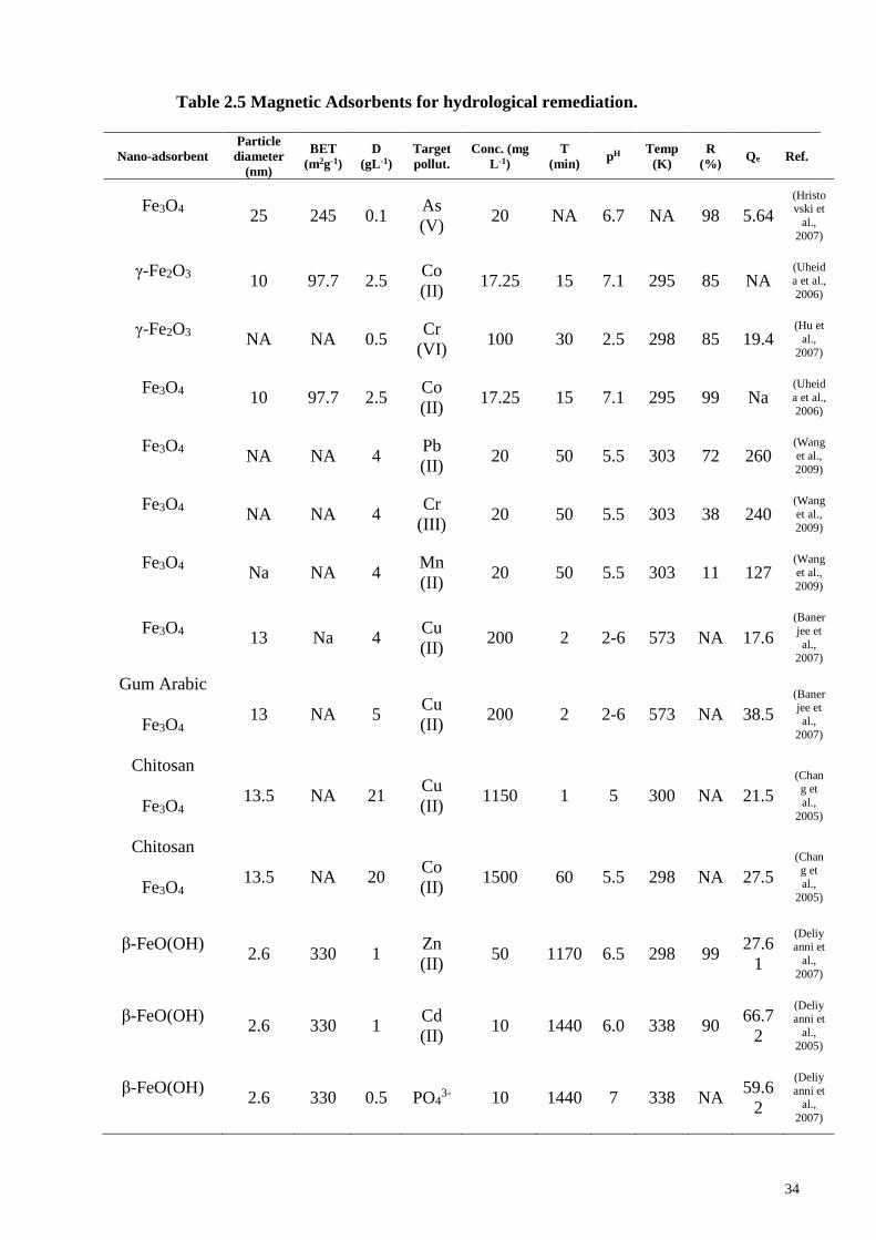
34
Table 2.5 Magnetic Adsorbents for hydrological remediation.
Nano-adsorbent
Particle
diameter
(nm)
BET
(m2g-1)
D
(gL-1)
Target
pollut.
Conc. (mg
L-1)
T
(min) pH
Temp
(K)
R
(%) Qe Ref.
Fe3O4 25 245 0.1
As
(V) 20 NA 6.7 NA 98 5.64
(Hristovski et
al.,
2007)
γ-Fe2O3 10 97.7 2.5
Co
(II) 17.25 15 7.1 295 85 NA
(Uheid
a et al.,
2006)
γ-Fe2O3 NA NA 0.5
Cr
(VI) 100 30 2.5 298 85 19.4
(Hu et
al.,
2007)
Fe3O4 10 97.7 2.5
Co
(II) 17.25 15 7.1 295 99 Na
(Uheid
a et al.,
2006)
Fe3O4 NA NA 4
Pb
(II) 20 50 5.5 303 72 260
(Wang
et al.,
2009)
Fe3O4 NA NA 4
Cr
(III) 20 50 5.5 303 38 240
(Wang
et al.,
2009)
Fe3O4 Na NA 4
Mn
(II) 20 50 5.5 303 11 127
(Wang
et al.,
2009)
Fe3O4 13 Na 4
Cu
(II) 200 2 2-6 573 NA 17.6
(Baner
jee et
al., 2007)
Gum Arabic
Fe3O4 13 NA 5
Cu
(II) 200 2 2-6 573 NA 38.5
(Banerjee et
al.,
2007)
Chitosan
Fe3O4 13.5 NA 21
Cu
(II) 1150 1 5 300 NA 21.5
(Chang et
al.,
2005)
Chitosan
Fe3O4 13.5 NA 20
Co
(II) 1500 60 5.5 298 NA 27.5
(Chang et
al.,
2005)
β-FeO(OH) 2.6 330 1
Zn
(II) 50 1170 6.5 298 99
27.6
1
(Deliyanni et
al.,
2007)
β-FeO(OH) 2.6 330 1
Cd
(II) 10 1440 6.0 338 90
66.7
2
(Deliy
anni et
al., 2005)
β-FeO(OH) 2.6 330 0.5 PO4
3- 10 1440 7 338 NA 59.6
2
(Deliy
anni et al.,
2007)

35
β-FeO(OH) 2.6 330 0.5
Cr
(VI) 50 432
5.5-
6.5 298 90 80
(Lazari
dis et
al., 2005)
HDTMA β-
FeO(OH) 4.6 231 0.5
As
(III) 30 1440 NA 298 NA 84
(Deliyanni et
al.,
2006)
HDTMA β-
FeO(OH) 4.6 231 0.5 PO4
3- 10 1440 7 338 NA 451
(Deliyanni et
al., 2007)
Fe(II) zeolite 4 21 10
As
(V) 20 1440 5-8 293 95 22.5
(Dousova et
al.,
2006)
Alumina 50 NA 3.5
Hg
(II) 94 42 NA NA 100 NA
(Pache
co et
al., 2006)
MnFe2O4 20 180 5
Cr
(VI) 100 60 2 298 100 NA
(Hu et
al., 2007)
MgFe2O4 20 70.3 5
Cr
(VI) 100 60 2 298 89 NA
(Hu et
al., 2007)
ZnFe2O4 20 79.6 5
Cr
(VI) 100 60 2 298 62 NA
(Hu et
al., 2007)
CuFe2O4 20 93.8 5
Cr
(VI) 100 60 2 298 49 NA
(Hu et
al., 2007)
NiFe2O4 20 101.2 5
Cr
(VI) 100 60 2 298 32 NA
(Hu et
al., 2007)
CoFe2O4 20 55.1 5
Cr
(VI) 100 60 2 298 20 NA
(Hu et
al., 2007)
ZrO2 20 45 0.1
As
(V) 20 NA 6.7 NA 85 3.97
(Hristo
vski et al.,
2007)
NiO 10 80 0.1
As
(V) 20 NA 8.4 NA 98 NA
(Hristovski et
al.,
2007)
NA = not available

36
2.2.15 Comparing adsorbents performance
The efficiency and effectiveness of the Nano-adsorbents was studied in comparison
to the conventional adsorbents to collect useful information to construct future water
purification systems. In this regards, the experimental parameters such as sample
solution pH, required adsorbent dose, adsorbates concentration, temperature (K) and
reaction time were compared to assess the performance of the Nano-adsorbents. Table
2.6 presents some adsorbents with high percent removal efficiency for the desired
environmental pollutants. For instance, the nitric acid treated MWCNT has far better
adsorption capacity for Pb (II) as compared to MnO2 coated MWCNT (Li et al., 2003;
Wang et al., 2007). The reason for such a difference of adsorption performance may be
ascribed to the generation of negative centers on the surface of MWCNT for effective
adsorptive interaction with metal cations. In batch adsorption studies times also plays
important role as it controls the steps involved during adsorption. In case of nitric acid
treatment four hours reaction time provide more adsorption capacity then MnO2 treated
adsorbent as only two hours were allowed to complete the adsorption process. In former
case the BET surface area was not reported while the second study reported a large BET
surface area as shown in the Table 2.1. The adsorbent particle sizes has shown
contradictory effect e.g. the particle size of MnO2-MWCNT is smaller than HNO3-
MWCNT but the percent removal and adsorption capacities are better in the second
case. The zero valent iron (Fe (0)) has more BET surface area than Kaolinite supported
Fe (0) Nano-adsorbent that provide 98 % adsorptive removal of Co (II) cations (Uzum
et al., 2009; Uzum et al., 2008). The incorporation of kaolinite with nZVI leads to
increase particle size from 8 to 300 nm as given in Table 2.6. Although nZI alone has
more surface area, still the Kaolinite supported nZVI adsorbent has almost doubled
adsorption capacity as it results in a 99 % removal efficiency of Co (II) of 100 mgL-1
initial concentration as compared to nZVI with 98 % removal of Co (II) with only 50

37
mgL-1, when the remaining experimental conditions were reported similar in the
individual studies (Uzum et al., 2009; Uzum et al., 2008). MCM 41 adsorbent has 99 %
removal efficiency for Cs with an initial concentration 2 mgL-1. The outstanding
adsorption capacity 179 mg g-1 may be related to the BET surface area as shown in the
Table 2.6.
The occurrence of Arsenic (As) in the surface or ground water at an increasing rate is
currently reported all over the world (Arcibar-Orozco et al., 2014; Smith et al., 2000). It
is estimated in different studies that As is affecting more than 100 million people all
over the world with increasing problem of polluted waters (Arcibar-Orozco et al., 2014;
Dixit et al., 2003). The World Health Organization (WHO) Arsenic established
maximum allowable limit is 10µgL-1(Bilici Baskan et al., 2010). The arsenic chemistry
elaborates that it is found in two oxidation states i.e. 3+ and 5+ (Anirudhan et al., 2013;
Dixit et al., 2003). The oxidation states are interchangeable with a relative change in
environmental pH, temperature, concomitant ionic species and oxidation reduction
conditions (Anirudhan et al., 2013; Bilici Baskan et al., 2010). Due to this reason one
form of Arsenic which is less toxic at present, can transform into more toxic state with a
change in environmental (Wang et al., 2014). There are different strategies to remove
Arsenic beyond permissible level in water supplies (Sen Gupta et al., 2009; Singh et al.,
2015; Trois et al., 2015). Adsorption is reported to be effective, efficient, easy,
economical and accessible technology (Anirudhan et al., 2013; Naseri et al., 2014).
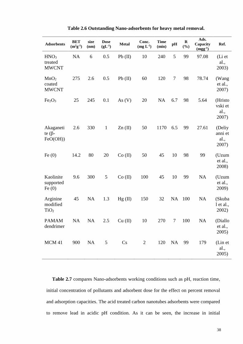
38
Table 2.6 Outstanding Nano-adsorbents for heavy metal removal.
Adsorbents BET
(m2g-1)
size
(nm)
Dose
(gL-1) Metal
Conc.
(mg L-1)
Time
(min) pH
R
(%)
Ads.
Capacity
(mgg-1)
Ref.
HNO3
treated
MWCNT
NA 6 0.5 Pb (II) 10 240 5 99 97.08 (Li et
al.,
2003)
MnO2
coated
MWCNT
275 2.6 0.5 Pb (II) 60 120 7 98 78.74 (Wang
et al.,
2007)
Fe2O3 25 245 0.1 As (V) 20 NA 6.7 98 5.64 (Hristo
vski et
al.,
2007)
Akaganeti
te (β-
FeO(OH))
2.6 330 1 Zn (II) 50 1170 6.5 99 27.61 (Deliy
anni et
al.,
2007)
Fe (0) 14.2 80 20 Co (II) 50 45 10 98 99 (Uzum
et al.,
2008)
Kaolinite
supported
Fe (0)
9.6 300 5 Co (II) 100 45 10 99 NA (Uzum
et al.,
2009)
Arginine
modified
TiO2
45 NA 1.3 Hg (II) 150 32 NA 100 NA (Skuba
l et al.,
2002)
PAMAM
dendrimer
NA NA 2.5 Cu (II) 10 270 7 100 NA (Diallo
et al.,
2005)
MCM 41 900 NA 5 Cs 2 120 NA 99 179 (Lin et
al.,
2005)
Table 2.7 compares Nano-adsorbents working conditions such as pH, reaction time,
initial concentration of pollutants and adsorbent dose for the effect on percent removal
and adsorption capacities. The acid treated carbon nanotubes adsorbents were compared
to remove lead in acidic pH condition. As it can be seen, the increase in initial

39
concentration from 10 to 20 mg L-1 has a negative effect on percent removal as it
decreases from 99 % to 75 % in these two comparative studies (Li et al., 2003; Lu et al.,
2006).
Table 2.7 Experimental conditions for Nano-adsorbents applications.
Adsorbents BET
(m2g-1)
Size
(nm) Dose Pollut.
Conc.
(mgL-1)
T
(hr) pH R% Qe Ref.
HNO3
treated
MWCNT
NA 6 10 Pb (II) 10 4 5 99 97 (Li et al.,
2003)
HNO3
treated
MWCNT
254 NA NA Pb (II) 20 1 3.5 75 91 (Lu et
al.,
2006)
Fe (0) 14.2 80 20 Co
(II)
50 0.7
5
10 98 99 (Uzum et
al.,
2008)
Activated
carbon
987 NA 4 Zn (II) 60 120 7 Na 20 (Leyva
Ramos et
al.,
2002)
Industrial
by
products
107 0.1 10 Ni (II) 249 8 4 90 32 (Gupta,
1998)
Industrial
by-
products
32 NA 2 Pb (II) 200 24 5.5 NA 32 (Feng et
al.,
2004)
Industrial
by
products
32 NA 2 Cu
(II)
200 24 5.5 NA 29 (Feng et
al.,
2004)
Agricultur
al waste
Na NA 9 Cu
(II)
126 NA 5 73 10 (Kadirve
lu et al.,
2001)
Agricultur
al waste
592 NA 0.4 Ni (II) 40 1 4 80 63 (Kadirve
lu et al.,
2001)
40
The other reason of this decline may be reduce reaction time or the use of more
acidic pH in the later study. This highlights the importance of experimental conditions
on the overall performance of Nano-adsorbents. Industrial by products offer an
economical alternate raw source of Nano-adsorbent. Industrial by products were
compared to remove Ni (II), Pb (II) and Cu (II) (Feng et al., 2004; Gupta, 1998). The
adsorbent show comparable adsorption capacity for Ni (II) and Pb (II) but a decline of
Cu (II) adsorption. Similarly, agricultural waste was reported to have better adsorption
capacity for Cu (II) but less than that of industrial byproducts (Kadirvelu et al., 2001).
In another study, a large BET surface area (592 (m2g-1)) removed 63 mg g-1 of Ni (II).
The superior adsorption capacity of agricultural waste over the industrial by products
(Table 2.7) supports the further studies to produce better adsorbents with large BET
surface area, functional groups, particle size with a competitive affinity for pollutants.
2.3 Modelling adsorption
2.3.1 Design of experiments
Central composite design (CCD), using the Stat ease 9.0 software, was selected to
plan for the adsorption experiments. The experiments were performed as suggested by
the software. Adsorption capacity (Qe mg.g-1) was calculated by following
(Shanmugaprakash et al., 2013).
𝑄𝑒 =(𝐶𝑜−𝐶𝑒)𝑉
𝑚 Equation 2.5
Where, Co and Ce stand for initial and equilibrium adsorbate concentration (mgL-1)
respectively, V is the total volume of solution in liters and m is the mass of adsorbent
(g). Adsorption experiments were repeated to check for systematic variations to
determine standard deviation and reproducibility of results. Four variables viz.
adsorbate initial conc. (mgL-1), pH, temp and Adsorbent (Ads. mg) in the range of 300-

41
500 mgL-1, 3.0 to 9.0, 20 to 40 and 400 to 600 (mg) respectively. In this work,
Equation 2.6, shows the selected quadratic model (Rehman et al., 2015).
𝑸𝒆 = 𝜷𝒐 + ∑ 𝜷𝒊𝒙𝒊
𝒌
𝒊=𝟏
+ ∑ 𝜷𝒊𝒙𝒊𝟐
𝒌
𝒊=𝟏
+ ∑ ∑ 𝜷𝒊𝒋
𝒌
𝒋=𝟐
𝒙𝒊
𝒌−𝟏
𝒊=𝟏
𝒙𝒋 + 𝜺 𝒊 ≠ 𝒋 Equation
2.6
Where βo is a constant coefficient, ε symbolizes error, xi and xj are independent
variables, βi, βii and βij represent coefficients of linear, quadratic and interaction effects
respectively. The data for each experiment was checked for the goodness of fit into the
statistical models. The verification of models was carried out by statistical tests i.e.
analysis of variance (ANOVA), residuals analysis (RA), scaling residuals (SR) and
prediction error sum of squares (PRESS) (Naseri et al., 2014). The verified and
validated models were applied to optimize the four input variables and to maximize
output i.e. fluoride, nitrates, nitrites, sulphates, phosphates, arsenic, cadmium, nickel,
iron and related heavy metals adsorption capacity.
2.3.2 Response surface methodology
Design of experiments (DOE) strategy is found as a superior method as compared to
one variable at a time “OVAT it strategy”, enables deeper insight into interactions
among pre-selected experimental variables (Rehman et al., 2015). The DOE strategy
applies collaborating experiments to minimize implementation cost of research and
development (Rehman et al., 2015). Normally, multiple interactions of variables and
non-linear behavior of adsorption process constitute a complex mechanism (Dora et al.,
2013). Until now, response surface methodology (RSM) is a competitive modeling tool
to analyze and present complex nonlinear relationships among variables either alone or
in combination and their synergistic or antagonistic effects on adsorption (Simsek et al.,
2013). Principle of RSM is to use polynomial equations in a programmed range to
discover optimum values and the best system response (Roy et al., 2014). All significant

42
experimental variables are co-varied over a pre-selected range to find combined
interactive effects and finally uniting all interaction results to build a mathematical
model (Rehman et al., 2015). Model can be implemented to improve adsorption
performance, reducing number of experiments and eradicating statistically insignificant
variables.
2.3.3 Adsorption Kinetics
Kinetics is the science which deals with the mechanisms and rates of chemical
reactions, and ideally kinetic models should be incorporated into geochemical models,
along with thermodynamics. From a thermodynamic study of a reaction we are unable
to say anything about how fast salt will dissolve in water. However there are complex
reaction taking place in the hydrosphere and it is important to know the kinetics of these
reactions to understand the complex interaction and mechanisms. Figure 2.7, shows the
three well known stages of adsorbate adsorbent interaction. The rate of these entire steps
controls the overall kinetics. The step taking more time to complete is known as the
slowest or the rate determining step. While identification of rate determining steps
offers an option to tailor the adsorption process. Adsorption kinetics provides useful
information about the mechanism of adsorption but also the speed of adsorption
reaction. A number of kinetic models are normally used to interpret the adsorption
mechanism e.g. pseudo-second order reaction, pseudo-first order reaction and
intrapaticle diffusion models.

43
Figure 2.7. The three stages of adsorbate-adsorbent interactions.
For the design of an effective hydro-decontamination system we need to know the
rate of chemical reaction taking place i.e. the rate of adsorption. With reference to
geochemical modelling, we do not attempt to explain in detail the broad field of
chemical kinetics, but just enough to understand the basics of kinetics. Several kinetic
models are implemented to examine the experimental data to decide on the nature,
intensity and mechanism of the adsorption process. The speed of adsorption was
evaluated by employing four kinetic models: pseudo-first order, pseudo-second order,
intraparticle diffusion and Banghams. The overall adsorption rate is proportional to the
driving force and the concentration gradient in the case of the first order, while in the
case of the second order, it is proportional to the square of driving force.
2.4 Challenges and role of adsorbents in remediation
Hydrology is concerned with the water properties, resources, resource conditions,
and water movement in relation to land along the dynamic environments (Dingman,

44
2015). While hydrological connectivity is determined by the presence of waterways,
hydraulic infrastructure, soil type, topography and geology to facilitate flow of water
across the land. Distribution pattern of water have a great influence on homing success,
the level of gene flow and population structure (Olsen et al., 2010). Environmental
fluctuations associated with water composition has a direct effect on all the depending
living beings e.g. fish, plants and the primary, secondary and tertiary consumers
(Chaparro et al., 2015). The global climate change, population increase, damming of
rivers, water abstractions and more water pollutants have exerted multiple pressures on
the water resources, aquatic and land ecosystem (Karthe et al., 2015). Occasionally, the
hydrological samples contain elevated levels of fluorides, nitrates, sulfates, phosphates,
chlorates, bromates, perchlorates and a number of heavy metals cause of serious
environmental issues and adverse impacts on public health (Bohlke et al., 1995; Kröger
et al., 2009; Pluta, 2001). Each geological regions have characteristic water availability
and water quality parameters, including turbidity, temperature, total dissolved solids
(TDS), pH, inorganic ions and organics and number of anthropogenic sources (Orem et
al., 2011).
Figure 2.8. Challenges and role of adsorbents in hydro-harsh environments.
The geological regions are unique and require some specific modification in the
water treatment systems. The environmental conditions have an influence on role of
adsorbents, stationary phases, water pollutants and CO2 capture, removal of organic and

45
inorganic species in routine or emergency situations as shown in Figure 2.8. For
example biological contamination and inactivation through biological fouling results in
decreased removal efficiency. A thorough understanding of the hydrosphere is
compulsory to design, manage and realize the global socio-economic developments
(Ruddell et al., 2015). The global water scarcity is an urgent and well-recognized
problem. The concept of water scarcity appears related with water quantity and quality
(Jiang, 2009; Zeng et al., 2013). However, without considering water quality criterion
the assessments and estimates of water scarcity is less precise and water quality has
become a critical factor with increasing number of pollutants (Zeng et al., 2013). Table
2.8 present current problem and issue with the use of adsorbents.
Table 2.8. General problems and issues of adsorbents (Karthe et al., 2015).
2.5 Research advancement in adsorbents protections
A number of research advancements have been observed in the literature in the past
decade. Table 2.9 presents some of the current research advancements in iron derived
adsorbents and protective measures as a contribution to advance the used or these
magnetic adsorbents under harsh environments. A common observation is the

46
aggregation of magnetic nanoparticles which leads to reduce efficiency as the effective
surface area is reduce by this behaviour of Nano-adsorbents.
Table 2.9 The protective measure for iron oxides.
# Research
advancement Adsorbent
Protective
measure Contribution Ref.
1 Preventing
aggregations Iron oxide
SDS surface
coatings
enhanced Arsenic
immobilizations
efficiency
(Kim et
al.,
2012)
2 Reduce particle
size Iron oxide
SDS surface
coatings
enhanced Arsenic
immobilizations
efficiency
(Kim et
al.,
2012)
3
Stability of
magnetic
particles in
acidic
environments
Iron oxide
sec-
octylphenoxy
acetic acid
(OPA)
Lanthanides
removal system
(Zhu et
al.,
2011)
4
Introducing
affinity for
nanoparticles
Iron oxide
polydimethyl
siloxanes
(PDMS)
enhance
hydrocarbon
adsorption
(Koniec
zny et
al.,
2008)
5
Environment
friendly
adsorbent
iron oxide
iron oxide
coated with
humic acid
efficient removal
of heavy metals
(Campos
et al.,
2011)
6
Smart
scavenger of
Hg (II)
gold
coating gold
particles with
citrate
avoids the
addition of
reducing agents
(Ojea-
Jiménez
et al.,
2012)
7
Thiol-
functionalizatio
n
Iron oxide
3-
mercaptopro
pyltriethoxys
ilane
(MPTES)
adsorption of
cadmium, lead and
copper ions
(Chen et
al.,
2012)
8
Ionic liquids in
hydrodecontam
inations
Iron oxide
Imidazolium
based ionic
liquid (IL)
reactive black dye
(Poursab
eri et al.,
2013)
9 Protected
adsorbents Iron oxide
Prussian blue
(K4[Fe
(CN)6])
removal of
radioactive cesium
(Cs)
(Thamm
awong et
al.,
2013)

47
Kim at al. reported that this issue can be resolved by the use of nanoparticle surface
coating with surfactants e.g. SDS coating (Kim et al., 2012). Secondly, this
development was also reported to reduce the effective particles size that enabled an
enhanced heavy metal immobilization from aqueous samples. Similarly, the problem of
stability in acidic environments were resolved by protective coating with sec-
octylphenoxy acetic acid (OPA) (Zhu et al., 2011). Konieczny et al found that magnetic
nanoparticles affinity for hydrocarbons removal can be amplified by coating with
polydimethyl siloxanes (PDMS) (Konieczny et al., 2008). The environmental friendly
humic acids (HA) coated Nano-adsorbents were developed to fulfill the
decontamination challenge by heavy metals pollution (Campos et al., 2011).
The use of reducing agents to prepare magnetic Nano-adsorbents makes these
methods environment non-friendly. This issue was resolved by coating gold particles
with citrate for making environment friendly mercury smart scavengers by avoiding the
use of chemical reducing agents (Ojea-Jiménez et al., 2012). Thiol functionalization of
iron nanoparticles by mercaptopropyl triethoxysilane (MPTES) provide suitable
magnetic modified Nano-adsorbent for heavy metals removal e.g. Cd, Pb and Cu (Chen
et al., 2012). Imidazolim based Ionic liquids were also reported to protect magnetic
Nano-adsorbents for organic dye removal from hydrological samples (Poursaberi et al.,
2013). Protected magnetic Nano-adsorbents have been also used for the remediation of
radioactive waste by the Prussian blue coatings (Thammawong et al., 2013).
The issues related to compatibility problems of nanotechnology materials with
natural environments include matric effects from environmental range of pH,
temperature, alkalinity, hardness, organics, inorganics, biological contaminants,
increase in industrial effluents and functionality loss with the extended use Table 2.8.
Aqueous streams with beyond permissible levels of heavy metals is regarded as one of

48
the most common problem in Malaysia (Fakhru’l-Razi et al., 2009). The attractive
energy efficient separation of magnetic adsorbents has been explored to open new
developments in the field of adsorbents for environmental treatment systems. Magnetic
anion exchange resin for the removal of reactive blue dye were considered superior due
to the easy magnetic separation (Shuang et al., 2011).The current literature review
provides an overview that how we can overcome some of the challenges by a careful
planning of adsorption system and protecting the magnetic Nano-adsorbents for an
extended use and stability to overcome the hydro-harsh condition that adversely affect
the separation efficiency, adsorption capacities in the extended adsorption/ desorption
cycles.
2.5.1 Socio-economic development and public health
The socio-economic development and improved public health is linked with the
supply of safe water. The rapid industrialization, urbanization and exponential increase
in population imposes burden to sustainability of limited natural resources. Earth
hydrosphere is facing evolving challenges by rigorous contamination from development
activities (Smith et al., 2000). The desire for improve living standards have highlighted
the needs for quantity and quality safe water. The awareness has risen gradually with
time to improve the quality of water to improve quality of life. The statistics about
population with access to safe water assumes ideal situations as they rely on perceived
fact while ignoring the ground realities (Onda et al., 2012). The superfluous
underestimate mislead the severity of water contamination problems, concerning public
health. The reason behind may be the difference in pollution levels or range of
contaminants concentration as indicator of the water quality in different geological
regions based on the availability of water. As the water flows across urban water supply
system it is continuously exposed to contaminants because of leakage or accidental
rupture of water pipes. Therefore, a continuous monitoring system is necessary to

49
monitor the fault of a particular water resource over the course of time. A continuous
attention and care is mandatory for better public health and social development (Onda et
al., 2012). The safe water usage practice is obligatory to realize the health gains from
water quality interventions. The distorted hygiene practices with even occasional
consumption of untreated drinking water results in the adverse public health issues. A
similar effort is the use of portable water treatment system at homes (Brown et al.,
2012). The household water pre-treatment (HWPT) is believed to prevent 500 disability
adjusted life years (DALYs) per 100,000 persons per year. The declining percentages of
HWPT tend to reduce the predicted health benefits (Brown et al., 2012). The fecal
contaminations of drinking water is a common cause of water-borne diseases (Kyle
Onda et al., 2013). World Health Organization (WHO) has documented various
drinking water quality parameters to assign safe status to consumer water. The improper
disposal of municipal, industrial wastes and indiscriminate applications of
agrochemicals challenges water quality. The Microbial or chemical pollutants remain
the main concern for better public health (Azizullah et al., 2011). It is crucial to
minimize the contamination of underground water, rivers, and lakes for the collective
survival of community members. The development of Nano-adsorbents offers the
possibility to resolve or greatly ameliorate the current problems plaguing water quality
(Qu et al., 2012).
Surface and ground water resources are often found to have elevated levels of
contaminants beyond the safe water quality level (Smith et al., 2000). The problem of
municipal and industrial waste, the massive output of agrochemicals from agricultural
practices, and natural disasters have become the main causes of declining water quality
(Azizullah et al., 2011). The present science desires to development chlorine-free
biocides to selectively target disease causing bacteria and viruses in water (Savage et
al., 2005). The desalination of saline water, recovery of toxic and valuable metals,

50
contaminants including perchlorate, pharmaceuticals, endocrine disrupters and chiral
compounds concerns present and future studies (Savage et al., 2005).
2.5.2 Resources scarcity
The basic problem is depletion of natural resources, massive exploration and rapid
changes in geochemistry. This situation is worsening by the increasing water demand of
population and the present pollution crisis. Further studies are mandatory to provide
some practical solutions for the changing definition of water scarcity. The all form of
life on the planet Earth gets benefits from the environment in the form of water, food
and shelter. Since the beginning of life the Earth is the nursery in which life developed
over billions of years (Postel et al., 2012). The natural hiccups in the environment occur
from time to time, but life continue to survive. There are two types of issues; the natural
and our own made environmental problem. The man made alteration in the
environments are thought to impose threat to the survival of life (Stevens, 1997). The
Earth provides the life support system and we must use it wisely not only for our
survival but also for coming generations (Young et al., 2009). At the present time we
have no other option to live on some other planets than Earth (Raymond et al., 2004).
There is a desire to preserve and protect the natural resources for sustainable health and
development. The contamination causes of hydrosphere must be checked and resolved
to carry forward the safe environment for future generation. Adsorbents purifying and
protecting materials have risen as a renewable, green and workable solution to protect
the natural hydrosphere. The expanding use of resources and industrial development is
necessary to fulfil the needs of increasing population but socio-economic development
must comply with the green environment for sustainable public health.

51
2.6 Comparative hydrological remediation
A number of remediation techniques are compared to evaluate the competency of
respective decontaminations strategies reported in the literature. The abundantly available
calcium hydroxide provides basic pH medium to precipitate Mn (II) with a 99.3 % removal
efficiency (Charerntanyarak, 1999). A comparison with coagulation with pol ferric sulfate for
Cu (II) removal shows that the previous technique require 10 mg L-1 optimum dose to
remove 1.09 mg L-1 while the later technique need more dose 25 g L-1. As it is clear the later
technique requires more adsorbent dose to accomplish a 99 % removal of Cu (II) from
hydrological samples. Nevertheless, the second technique remove 20 mg L-1 of Cu (II) that is
far high concentration of pollutant as compared to the previous technique (Li et al., 2003).
The role of ionic surfactants to remove Zn (II) cations from hydrological samples is
compared by the use of surfactant 105 and sodium dodecyl sulfate (SDS) in two separate
studies (Matis et al., 2004; Zouboulis et al., 2003). In these two flotation methods the SDS
surfactant displayed better removal of Zn (II) as compared to Surfactant 105, as it remove
0.05 mg L-1(Table 2.10). Interestingly, the synthetic zeolites demonstrated 100 % removal
efficiency for Cr (III), Ni (II) and Zn (II). As compared to ultrafiltration the nanofiltration
with polyamide remove 200 mgL-1 of Cd (II) with a 99 % removal efficiency (Abu Qdais et
al., 2004; Juang et al., 2000). The reverse osmosis techniques was compared to remove Cu
(II) and Ni (II) metal cations with a ES20 membrane (Ozaki et al., 2002). Similarly,
membrane electrolysis provided 99.6 % removal efficiency for Cr (VI) by iron rotary with
130 mg L-1 pollutants initial concentration in basic pH 8.5 (Martinez et al., 2004). Table 2.10
also compared metals removal efficiency of adsorption technique for Pb (II), Zn (II), Hg (II)
and Co (II), with different adsorbent dosages ranging from 0.5 g to 5.0 g. It can be seen from
the comparison results that with the use of more adsorbent dosage the percent removal
efficiency increases linearly because of the availability of more surface sites for interaction

52
with the hydrological pollutants (Deliyanni et al., 2007; Skubal et al., 2002; Uzum et al.,
2009; Wang et al., 2007). Figure 2.9 provide a clear picture of the relative remediation
performance in terms of adsorption capacities. The available activated carbon, industrial by
produces and agricultural waste has comparable adsorption capacities for heavy metals. On
the other side advanced supports e.g. MWCNT, MCM-41 and magnetic nZVI are
demonstrating the high adsorption capacity as compared to conventional adsorbents. It
clearly supports the use of advance materials for further research as it is evident from the
literature review study.
Figure 2.9 Remediation performance of conventional and Nano-adsorbents.

53
Table 2.10 The comparative removal efficiency of remediation techniques.
Remediation
technique
Environ.
Pollutant
Remediation
source
dose
(gL-1)
Conc.
(mg L-1) pH R (%) Reference
Chemical
precipitation
Mn (II) Ca (OH)2 10 1.085 11 99.30 (Charerntanyarak,
1999)
Coagulation Cu (II) Poly ferric
sulfate
25 20 10-
11.5
99 (Li et al., 2003)
Floatation Zn (II) Surfactin
105
0.04 50 6 100 (Zouboulis et al.,
2003)
Floatation Zn (II) SDS 0.05 50 7-9 100 (Matis et al.,
2004)
Ion exchange Cr (III) zeolite 2.5 100 NA 100 (Alvarez-Ayuso et
al., 2003)
Ion exchange Ni (II) Synthetic
zeolite
2.5 100 NA 100 (Alvarez-Ayuso et
al., 2003)
Ion exchange Zn (II) zeolite 2.5 100 NA 100 (Alvarez-Ayuso et
al., 2003)
Ultra-
filtration
Cu (II) YMI NA 79 8.5-
9.5
100 (Juang et al.,
2000)
Nanofiltration Cd (II) Polyamide NA 200 4-11 99 (Abu Qdais et al.,
2004)
Reverse
osmosis
Cu (II) ES20 NA 50 7-9 100 (Ozaki et al.,
2002)
Ni (II) ES20 NA 50 7-9 100 (Ozaki et al.,
2002)
Membrane
electrolysis
Cr (VI) Iron rotary NA 130 8.5 99.60 (Martinez et al.,
2004)
Adsorption Pb (II) MnO2
coated
MWCNT
0.5 60 7 98 (Wang et al.,
2007)
Adsorption Zn (II) Akaganetite 1 50 6.5 99 (Deliyanni et al.,
2007)
Adsorption Co (II) Kaolinite
supported
Fe (0)
5 100 10 99 (Uzum et al.,
2009)
Adsorption Hg (II) Arginine
modified TiO2 1.33 150 NA 100 (Skubal et al.,
2002)
54
2.7 The competitive adsorption technique
The competency or preference of adsorption over other techniques relies on the
involvement of surface phenomenon that can be fine-tuned to remove contaminants or
the dissolved solutes from samples e.g. Industrial wastewater, polluted river and
drinking water. Desorption is the process to remove adsorbed solute on the surface of
adsorbent by the use of a suitable elution solvents e.g. acids, bases, ionic liquids,
organic solvents or technique such as sonication, microwave or calcination. The
opportunity to desorb contaminants from the surface of adsorbents paves the way to
recycle and reuse of adsorbents. Water treatment techniques apply adsorbents as an
effective, alternative and practical solution to remove contaminants (Crini, 2006). The
extended applications include product purification, storage or capturing organics,
chromatographic stationary phases, and removal of pollutants (Hicks et al., 2008;
Rehman et al., 2015; Wang et al., 2011; Xu et al., 2002). The need-based adsorbents
have sparked interest throughout the scientific community along with an allusive
challenge of competency and stability during harsh environmental conditions (Jeremias
et al., 2012; Zhang et al., 2011). The rational design of adsorbents with prolonged
stability in environmental stress conditions has lead towards the curiosity and search for
more adsorbents (Masters et al., 2011). The manifestation of unforeseen disasters, such
as earthquakes, floods and mega natural disasters highlight the need for straightforward
adsorbents (Mahmood et al., 2011). The interest to make smart, portable water treatment
devices with minimal energy consumption follows the developments in separation
sciences applications (Baig et al., 2011; Mwabi et al., 2011). Water crisis in different
geological regions of the planet has called for research to ensure superior adsorption
capacity, magnetic separation and prolonged stability (Chaturvedi et al., 2012).
Fortunately, the synthetic revolution in Nano-adsorbents and advanced characterization

55
techniques provide deep insights into the modified Nano-adsorbents (Rehman et al.,
2015). Future research is dedicated to collective consequences from water chemistry,
nanoparticles characteristics and their coating condition, performance of supports and
adsorbents (Crini, 2015). We realize that the adherence to green approaches in
pollutants removal techniques provides the roadmap for the future developments
(Husain et al., 2015; Rezaei et al., 2015).
The feasibility of adsorption desorption cycles depends on the nature of adsorbent-
adsorbate interaction. For example, there are two types of complex formation (a) Inner
sphere complexes (ISC) (b) Outer sphere complexes (OSC). In case of ISC formation
intense chemical bonding takes place and recycling is more challenging and require
stringent desorption conditions or chemical, while in case of OSC the surface
phenomenon is governed by the dominant physical forces of attraction holding the
participants together through relatively weaker forces (Huang et al., 2008). In OSC the
reuse and regeneration process is exercised to maintain the overall cost by reusing the
materials over extended period of times (Loganathan et al., 2013). The regeneration and
reuse of Nano-adsorbents is one of the crucial aspects as it controls the economy of the
hydro-decontamination technologies. Many researchers has attempted to regenerate and
recycle Nano-adsorbents, as it become the hot spot of the separation sciences. An
understanding of the mechanism and chemistry of separation reactions helps to bring
out novel ways to regeneration and reuse. Recent literature shows the use of various
reagents such as acids, alkalis and chelating agents for application in the regeneration of
adsorbents for extended economical usage. A comparison between the past and present
research indicates, various number of studies reported on adsorbent that can be recycled
several times for recycling and reuse (Table 2.11). The number of time a specific
adsorbent recycles seems to be dependent on the stability of the adsorbent. The ferri-
hydride adsorbent demonstrated an unchanged efficiency even after 50 times of

56
regeneration and reuse cycles by controlling the pH of the medium to regenerate the
adsorbents (Edwards et al., 1989). The graphene hydrogel and hydro-talcites were
studied unto 10 regenerations with pH control, salt solution and organic solvent such as
ethanol (Gao et al., 2013; Kuzawa et al., 2006). The chelating agents such as ethylene
di-ammine tetra acetic acid (EDTA) can be used to regenerate magnetic bio-char based
adsorbent for six consecutive cycles, however the adsorbent efficiencies were reported
to decreased after each cycle (Wang et al., 2015). Normally, pH control of the solution
by the use of appropriate amounts of acids or alkalis can be used to regenerate a number
of adsorbent such as Chitin based adsorbents, cement adsorbents, clay adsorbents,
chitosan, maghemite, zeolites and functionalized silica (Han et al., 2009; Hu et al.,
2005; Kamble et al., 2007; Kundu et al., 2005; Liu et al., 2000; Mandal et al., 2009;
Thakre et al., 2015). Organic solvents (e.g. n-hexane) were used to dissolve organic
pollutants such as dyes and the organics adsorbed on the surface and regeneration of the
exhausted adsorbents on the simple principal of solvent extraction (Ma et al., 2013).
Asghar et al. reported an electrochemical regeneration method for un-treated and treated
graphite based adsorbents (Asghar et al., 2013). At the anode, the oxidation of adsorbed
dye acid violet 17 leads to the regeneration.
The high regeneration efficiency (100%) was reported over five adsorption/
regeneration cycles for the un-treated and treated graphite. Besides this method involve
the formation of several breakdown products during electrochemical oxidation of
organic dye (Asghar et al., 2013).The most important aspect in regeneration and reuse
strategy is a wise reuse of the desorbed concentrated amounts of organic or inorganic
pollutants along with the recycled adsorbents. The best way of disposal management is
to avoid Nano-toxicology and reuse of the desorbed pollutant in the relevant industry
for the manufacture of various commodities (Ali, 2012). The regenerated metals may be
reused in the metal processing industries.

57
Table 2.11 Adsorbents regeneration methods.
# Type of
adsorbents
Regeneration
method
No of
reuse
(times)
Effect on
efficiency Ref.
1 Ferri-hydride pH control 50 unchanged (Edwards et al.,
1989)
2 Hydro-talcite Salt and pH
control 10 decreased
(Kuzawa et al.,
2006)
3 Functionalized
Silica pH 03 decreased (Liu et al., 2000)
4 Zeolites pH 03 decreased (Han et al., 2009)
5 Graphene
composite Annealing 05 unchanged (Geng et al., 2012)
6 Maghemite pH 06 unchanged (Hu et al., 2005)
7 Graphene
hydrogels pH and ethanol 10 decreased (Gao et al., 2013)
8 Chitosan pH 03 decreased (Kamble et al.,
2007)
9 Porous
desiccants Microwave - - (Inglis et al., 1989)
10 Activated
carbons Microwave 06 Increased (Ania et al., 2004)
11 Super adsorbent
polymer Photo catalytic - decrease
(Dhodapkar et al.,
2007)
12 Clay pH 05 decreased (Mandal et al., 2009)
13 Graphene
composite ethylene glycol 05 Decreased (Sun et al., 2011)
14 Zeolite Microwave 03 slight
decrease (Han et al., 2010)
15 Phosphate
adsorbent Ion exchange 20 decrease (Urano et al., 1992)
17 Chitin base
adsorbent pH - decrease (Thakre et al., 2015)
18 Activated
carbon Ethanol/ NaCl 05 Suppressed (Du et al., 2015)
19 Magnetic bio char EDTA 06 decrease (Wang et al., 2015)

58
2.8 Summary of the literature review
Magnetic and Nano-adsorbents have been proven as effective measure for treating
contaminated environment for green environment remediation. The high chemical
consumption and treatment cost is reduced by the application of renewable adsorbents
resources. The research of novel series of adsorbents by a number of preparation routes
provides a solution to meet the increasing safe water requirement of the population. The
poor socioeconomic conditions and generation of large volume of industrial and
agricultural waste are the major challenges of the present time. The CCD modelling
tools can be applied to model the adsorption process. The application of kinetic studies
provides some basic information regarding the speed of pollutants removal during field
applications. The emergence of novel composite adsorbents by the composite with
grapheme oxide and carbon nano tubes offers practical advantages in adsorbent
applications. A large number of composites formats were reviewed to compare the
relative percent removal efficiency of some of the advance forms of adsorbents in this
study.

59
CHAPTER 3: RESEARCH METHODOLOGY
The success of green environmental remediation is dependent on the
reliability of data, design of work, experimentation, application of precise and
accurate research methodology. Normally, geological features of the study area are
well documented by field observation followed by mechanical, physical and chemical
analysis to interpret the causes of a particular environmental problem. In this regards,
the geochemical models are efficient and selective in terms of large scale data
presentation, three dimensional maps building through the use of vector and raster
data. The interpretation of geochemical model identifies the environmental issue and
local point pollution resources e.g. industrial waste, hospital waste or house waste.
The identified problem is resolved by the application of magnetic Nano-adsorbents by
following OVAT or DOE strategies to reduce time, cost and efforts. Well-planned
and performed experiments ordinarily give reproducible and reliable data.
This chapter describes the materials as well as the methodology used in the study.
The sampling methods, research instruments and statistical procedures to collect,
analyze, interpret the data and findings are also presented. The experimental setup used
to make magnetic Nano-adsorbents via mechanical milling, sol-gel method, micro-
emulsions, co-precipitation, various analytical and spectroscopic techniques for
adsorbents characterization and hydrogeological applications are described. All
experiments are distinctive from each other and in each situation standard procedures
were followed for data collection, interpretation and presentation. The experimental
parameters were optimized through two strategies: one variable at a time (OVAT) as
well as design of experiment (DOE). The adsorption experiments were repeated at least
three times to establish the reproducibility of the experimental results. Maximum care is

60
taken in the design, conduct, collection and analysis of experimental results. The
following section will discuss the materials and methods employed in this study.
3.1 Materials
In this work, the AR grade reagents with high purity were used as listed in
Table 3.1. Acetonitrile (ACN), Water and Methanol of HPLC grade were purchased
from Merck, Germany, and used for making Acephate aqueous solutions and for
HPLC method. Throughout the experiments, all glassware was cleaned with 20%
nitric acid and repeatedly washed with deionized water, followed by drying at 373K
in an oven for 5 h. The samples of required concentrations were prepared by diluting
the stock solution. The buffers of pH (1–3), (4–6) and (7–10) were prepared by
mixing an appropriate volume of 0.1M solutions of HCl–KCl, CH3COOH–
CH3COONa and H3BO3–NaOH, respectively [D. Perrin 1974]. In this work, de-
ionized water (18.2 MΩ-cm at 25 °C) was used for preparing working and standard
solutions.
3.2 Preparation of magnetic adsorbents
Magnetic adsorbents play a very important role in hydrogeological
decontaminations, separation, physical and materials sciences. The superior physical,
chemical, thermal, electrical, optical and magnetic properties attract extensive
applications in green environmental remediation, removal of pollutants from drinking
water, river water and polluted water resources. In this context, preparation of
adsorbent is a very important assignment for material scientists. In this work, we have
fabricated the different series of adsorbents by the hydrothermal, sol-gel method,
micro-emulsions, co-precipitation, and mechanical milling methods.

61
Table 3.1: List of chemicals
Name Formula Company Purity (%)
Copper nitrate Cu (NO3)2 Merck >99
Ferrous nitrate Fe(NO3)2 Merck >99.5
Ferric nitrate Fe(NO3)3 Merck >99.5
Potassium Ferro cyanide K4[Fe(CN)6] Merck >99.5
Potassium Ferri cyanide K3[Fe(CN)6] Merck >99.5
Sodium hydroxide NaOH Merck >99.5
Potassium chloride KCl Merck >99.5
Ammonium hydroxide NH4OH Merck >99.5
Sulphuric acid H2SO4 Merck >99.5
Hydrochloric acid HCl Merck >32
Nitric acid HNO3 Merck >69.5
Phosphoric acid H3PO4 Merck >75.5
Potassium di-chromate K2Cr2O7 Merck >99.5
Carbon flakes C Sigma Aldrich >99.5
Cerium ammonium nitrate (NH4)2Ce(NO3)6 Merck >99.5
Monosodium phosphate NaH2PO4 Merck >99.5
Disodium phosphate Na2HPO4 Merck >99.5
Acephate C4H10NO3PS Merck >99.5
Methylene blue C16H18N3SCl Merck >99.5
Methyl orange C14H14N3NaO3S Merck >99.5
n-hexane C6H12 Merck >99.5
Boric acid H3BO3 Merck >99.5
Acetic acid CH3COOH Merck >99.5
hexadecyl-trimethyl-ammonium
bromide (CTAB) C19H42NBr Merck >97.0
Phenosephranine
3, 7-Damino-5-
phenylphenazinium
chloride
Sigma Aldrich >99.5
Gadolinium nitrate hexahydrate Gd (NO3)3.6H2O Sigma Aldrich >99.5
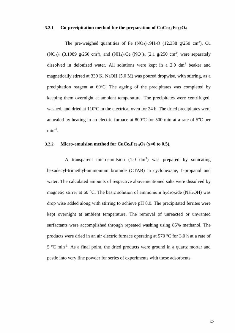
62
3.2.1 Co-precipitation method for the preparation of CuCe0.2Fe1.8O4
The pre-weighed quantities of Fe (NO3)3.9H2O (12.338 g/250 cm3), Cu
(NO3)2 (3.1089 g/250 cm3), and (NH4)2Ce (NO3)6 (2.1 g/250 cm3) were separately
dissolved in deionized water. All solutions were kept in a 2.0 dm3 beaker and
magnetically stirred at 330 K. NaOH (5.0 M) was poured dropwise, with stirring, as a
precipitation reagent at 60oC. The ageing of the precipitates was completed by
keeping them overnight at ambient temperature. The precipitates were centrifuged,
washed, and dried at 110oC in the electrical oven for 24 h. The dried precipitates were
annealed by heating in an electric furnace at 800oC for 500 min at a rate of 5oC per
min-1.
3.2.2 Micro-emulsion method for CuCexFe2-xO4 (x=0 to 0.5).
A transparent microemulsion (1.0 dm3) was prepared by sonicating
hexadecyl-trimethyl-ammonium bromide (CTAB) in cyclohexane, 1-propanol and
water. The calculated amounts of respective abovementioned salts were dissolved by
magnetic stirrer at 60 oC. The basic solution of ammonium hydroxide (NH4OH) was
drop wise added along with stirring to achieve pH 8.0. The precipitated ferrites were
kept overnight at ambient temperature. The removal of unreacted or unwanted
surfactants were accomplished through repeated washing using 85% methanol. The
products were dried in an air electric furnace operating at 570 oC for 3.0 h at a rate of
5 oC min-1. As a final point, the dried products were ground in a quartz mortar and
pestle into very fine powder for series of experiments with these adsorbents.

63
3.2.3 Hydrothermal reductive fabrication of CuCe0.2Fe1.8O4-rGO
Graphene sheets were prepared using a modified Hummer’s method
(Azarang et al., 2015). The process began with the oxidation of graphite flakes by
adding sulfuric acid and phosphoric acid (4:1 v/v) at room temperature. A weighed
quantity of potassium permanganate (KMnO4) was added slowly, and then
continuously stirred with a magnetic stirrer for three days to complete the oxidation
process. The chemical oxidation reaction was stopped by the addition of hydrogen
peroxide (H2O2), along with ice cubes, to keep the temperature to a minimum, which
immediately formed yellow precipitates. A neutral pH condition was achieved by
successively washing the precipitates with hydrochloric acid (HCl) several times to
yield the final product: exfoliated graphene oxide (GO). For the preparation of the
graphene-based CuCe0.2Fe1.8O4 nanocomposites, graphene oxide (GO) (10.0 mg) was
dissolved into 50.0 cm3 of deionized water and sonicated for about 20 min to obtain a
clear solution. Similarly, CuCe0.2Fe2O4 nanoparticles were dissolved in water by
sonication, and mixed into the GO solution as shown in Figure 3.1. The above-
mentioned solutions were transferred into a Teflon-lined stainless steel autoclave and
heated for 480 min at a heating rate of 5oC per min in an electrical heating furnace.
Following this, it was cooled, centrifuged and washed several times with deionized
water. The graphene-based CuCe0.2Fe1.8O4 nanocomposites were then dried in an
oven at 60oC overnight.
Figure 3.1. The scheme of hydrothermal reduction.

64
3.2.4 Mechanical milling to form grades of POCS
Mechanical milling was used to prepare three grades of POCS:
i. Well graded
ii. Uniformly graded and
iii. Gap graded adsorbents from palm oil industrial waste.
The factory rejected waste materials were fed to a mechanical mill to obtain the
particles of various sizes, followed by the separation of each type of particles according
to the US standards sieving process. A standard criteria for well graded POCS is
illustrated as in Figure 3.2.
Figure 3.2. Mechanical grades of POCS by US standard sieving.

65
Equation 3.1. Uniformity coefficient of adsorbents.
𝐶𝑢 =𝐷60
𝐷10
Equation 3.1
Where Cu is the uniformity coefficient of the particles and should be greater than 4-6,
D10, D60 corresponds to particles diameter of 10 % or 60 % finer respectively and is
accepted as the effective size. The effective size of adsorbent particles is a good
measure to estimate the hydraulic conductivity and drainage (Das, 2010). In Fig. 3.2, the
blue curve represents the adsorbents with well graded adsorbents particles (0.1 mm to
5.0 mm). The coefficients Cu and Cz for the blue curve are 10.67 and 1.13 respectively
satisfy the criterion for well graded adsorbents particles prepared by the mechanical
milling process. The second criteria for well graded adsorbents is the coefficient of
gradation (Cz)
Equation 3.2. Coefficient of gradation.
𝐶𝑍 =𝐷30
2
𝐷60 𝑋𝐷10
Equation 3.2
The desirable range of Cz for the adsorbent particles is between 1-3. The POCS (red
curve) shows a very narrow range of particle size from 0.6mm to 2.3mm. The value of
coefficients Cu, Cz is 2.28 and 0.77 respectively. From these values it is clear that the
particles have different sizes with a gap represented by a linear trend. The POCS (green
curve) consists of nearly uniform particles as shown by the graph. The high value of (Cu
~ 29) and least value of (Cz ~ 0.11) conforms to the uniformly graded adsorbents.

66
3.3 Characterization of fabricated Nano-adsorbents
The successful chemical synthesis of Nano-adsorbents can be judged by the
yield and the homogeneity of the product. The materials performance is certified by
using analytical and spectroscopic techniques. The characterization of Nano-
adsorbents is an important part in the determination of functional groups, shape, size,
phase purity, optical band gap and chemical composition. In the present work, the
synthesized adsorbents are calcined at dissimilar temperatures and are structurally
characterized by different spectroscopic and analytical techniques such as powder X-
ray diffraction (XRD), X-ray photoelectron emission spectroscopy (XPS), Raman
Spectroscopy, thermogravimetric analysis (TGA), scanning electron microscopy
(SEM)/ energy-dispersive X-ray spectroscopy (EDS), High resolution transmission
electron microscopy (HRTEM), Fourier transform infrared spectroscopy (FTIR) and
ultraviolet– visible spectroscopy (UV-Vis).
3.3.1 Powder X-ray diffraction (XRD)
Powder XRD method is commonly exploited for characterization of Nano-
adsorbents. In this method the materials to be analyzed is grinded to a very fine
powder by a quartz mortar pestle and spread on the sample holder to feed into the
beam of monochromatic X-rays. Each particle in the sample is a tiny crystal randomly
oriented with respect to the incident X-rays. The tiny crystals reflect light at different
2-theta scale depending on the lattice plans (Chung, 1974). The reflected beam
position and intensity is recorded for comparison with a known standard. This
comparison delivers the information regarding the crystallinity, crystalline size,
crystal stress or crystal strain, solid solutions and amorphous content of the sample.
XRD is used to confirm the formation of solid state reaction, purity of phases, lattice
constants, inter-planar distances, composition of elements at the octahedral and

67
tetrahedral sites (Suryanarayana et al., 2013).
Mathematically, the average crystallite sizes can be determined by using the
Debye-Scherrer’s formula Equation 3.3.
𝐷 = 𝐾𝜆
𝛽ℎ𝑘𝑙𝐶𝑜𝑠𝜃 Equation 3.3
Where, D is the crystal size perpendicular to the reflection plane, K is the
unit cell geometry dependent constant and its value is typically between 0.85-0.99, ʎ
is the wavelength of X-rays radiations by the equipment (1.5418 Å), βhkl is the
broadening of the diffraction line measured at half the line maximum intensity (full
width at half maxima; FWHM) and θ is the angle between the incident X-rays and the
reflection plane (2θ/2). The Bragg βhkl can be written as Equation 3.4.
𝛽ℎ𝑘𝑙 = (𝐵ℎ𝑘𝑙 − 𝑏) Equation 3.4
Where, βhkl is the broadening measured on the X-ray pattern, and b is the
broadening error of the equipment, a typical of each instrument. The X-ray powder
diffraction spectra determines the lattice constants, phase nature, purity and crystal
structure of synthesized magnetic Nano-adsorbents. The XRD analysis was
performed using PANanalytical X-ray diffraction model Almelo, The Netherlands
equipped with HighScorePlus (Version: 3.od (3.0.4 and License Number 10003698,
Chemistry department, University of Malaya) software for data processing and
analysis. The samples were finely grinded before placing on the sample holder with a
gentle tapping to make a uniform powder layers. The sample holder was placed in the
labelled samples vertical stage for identification. A continuous 2θ scan mode from
10o-95 o was used for whole range scan. A divergence slit ensure that the X-rays

68
focused only on the sample. The diffractograms were matched with the Joint
Committee on Powder Diffraction Standards (JCPDS) PDF 1 database 2.6 to confirm
the identity of samples (Figure 3.3).
Figure 3.3. Garnet ferrites diffractogram showing 100% phase purity.
3.3.2 Thermogravimetric analysis
Thermogravimetric analysis (TGA) is an analytical technique that employs
thermobalance to monitor changes in the weight of a sample as the temperature
increases in the preselected programmed temperature range e.g. 50 oC to 900 oC. The
thermogram is the graph that shows the pattern of weight loss. Each downfall in the
thermogram indicates a degradation of sample, evaporation of water, decomposition
or formation of certain phases. The thermogram is used to evaluate quantity of
components, weight loss and thermal effects during the conversion of precursors to
final metal oxides Nano-adsorbents.
The thermal strength of the magnetic Nano-adsorbents was assessed by
using a computer programmed thermobalance equipped with a supply of inert gas
(N2), located at the central equipment facility, chemistry department university of

69
Malaya. An approximate weight (~10 to 50 mg) of each materials was taken into the
ceramic cup and placed inside the thermobalance followed by a lid on the top to
provide an isolated environment. The software options were selected dynamically
from ambient to 900oC at a heating rate of 10 oC min-1 under nitrogen gas with a flow
rate of 20 ml min-1. For second sample the thermobalance automatically cools down
to room temperature before being heated again from ambient to 900oC at a heating
rate of 2 oC min-1 with the same gas flow rate.
3.3.3 Electron microscopic analysis
Electron microscopy analysis tender structural information along a range of
magnifications as compared to a simple light microscope from 10 μm to 0.2 nm,
specifically for the minute quantity or tiny fragment of magnetic Nano-adsorbents
particles at a time when optical microscopes are unable to image it to any further
extent. The modern electron microscopes work in either transmission or reflection
mode to view the particles of magnetic Nano-adsorbents. The primary principle or
plan of each operative approach are discussed as follows.
3.3.3.1 Scanning electron microscopy (SEM)
Scanning electron microscopy (SEM) is one of the versatile and well known
exploratory techniques (Tung et al., 2009). Compared to the old-fashioned optical
microscope, an electron microscope offers high magnifying capability, high
resolution, and inspection of Nano-adsorbents or simplicity of sample preparation.
Electrons fired by an electron gun enter the surface of the sample and produce several
low energy secondary electrons. The intensity of the secondary electrons is governed
by the surface features and nature of the sample. Consequently, image is constructed
by determining the secondary electron as a function of the location of the incidental
electron beam (Cahn et al., 2013).

70
In addition to secondary electrons, backscattered electrons, Energy
Dispersive X-ray (EDS) analysis delivers useful information about the magnetic
Nano-adsorbents particle sizes, distribution and aggregation. In case of backscattered
electrons imaging the intensity of the backscatter electron, generated by electron
bombardment is correlated to the atomic number of the element, revealing the identity
of the constituents’ elements and percent composition of the magnetic Nano-
adsorbents. The fingerprints X-rays emitted from the component elements aid in
deduction of elemental information of the magnetic Nano-adsorbents. It also serves
chemical elements mapping along the entire surface and a semi quantitative analysis.
At present, these analytical techniques are frequently used for non-destructive surface
analysis, material characterization and wide applications in research and industry.
3.3.3.2 High resolution transmission electron microscopy
HRTEM is an indispensable technique for nanomaterials and
nanotechnology for the determination of fine structure, shape and lattice properties at
a very high resolution. In this technique, transmitted or forward-scattered electron
beam interacts with a solid particles, creating a number of elastic or inelastic
scattering. Further, the beam passes through a succession of lenses that determines the
image resolution. The source electron beam is produced by current heating of cathode
filament. TEM requires high vacuum for the travelling of electrons from cathode to
anode. A supporting accelerating voltage is applied between 50 to 150 kW, to control
the electrons and image resolution. The higher accelerating voltage provides shorter
electron waves for high image resolution of the samples particles. The accelerated
electrons reach to the bottom anode, following a similar way to that of light in an
optical microscope. The electrons are focused by a condenser onto the object, where
they are partially deflected after collision with the nanoparticles. The degree of

71
deflection varies according to the electron density of the nanoparticles. Generally, the
greater the mass of the particles, the greater is the degree of electrons deflection. The
scattered electrons are collected on an objective lens creating an image that is
magnified by an additional system of lenses. The final processed image is visible on
the computer screen, ready for saving into image file formats. In the present study,
LEO-Libra 120 (Germany) transmission electron microscope is used to study the
morphology of the products.
3.3.3.3 Surface analysis of Magnetic Nano-adsorbents
The surface morphology of the samples was studied by using a Quanta 200
FEI FESEM instrument and EDS was used to analyze the chemical composition of
the sample surface. The powder samples were adhered to the aluminium sample
holder using a small piece of carbon conductive tape before they are loaded into the
sample chamber of the instrument. The air evacuation in chamber was performed
before analysis. The EDS were analyzed using INCA-Suite version 4.02 software.
The detailed parameters of the measurement were as follow:
Working distance : 8-10 mm
Vacuum mode : High vacuum
Accelerating voltage : 5 kV
Spot size : 2.5 – 3 µm
Detector : Large Field Detector (LFD)
For measurement of the elemental composition of the samples the
acceleration voltage was focused on the sample dispersed on carbon tape fixed on
sample holder. The TEM specimens were prepared by dropping the samples on a
copper grid. For the size measurement and phase identification, images of
representative areas of the sample were taken at different magnifications with a CCD

72
camera.
3.3.4 Fourier Transform Infrared Spectroscopy (FTIR)
Fourier Transform Infrared Spectroscopy (FTIR) is an analytical technique
used to identify the functional groups present in the sample (Stuart, 2005). The FTIR
spectrophotometer is used to measure the absorption of various infrared light
wavelengths by the material of interest. The infrared absorption bands are used to
identify a specific functional group. The early-stage IR instrument dispersive infra-
red light through a prism or a grating monochromator (Sheppard, 2006). The scanning
rate of these pioneers’ instruments was slow requiring more time for the analysis of
samples. The latest Fourier Transform Infrared (FTIR) spectrometer work faster. A
typical FTIR spectrometer obtains infrared spectra by collecting an interferogram of a
sample signal with an interferometer, which measures all of infrared frequencies
simultaneously (Stuart, 2005). The acquired interferogram is digitized by Fourier
transform function to build an output FTIR spectrum (Stuart, 2005). The infrared light
can be categorized as far infrared (4~400 cm-1), mid infrared (400~4,000 cm-1) and
near infrared (4,000~14,000 cm-1). When an infrared ray interacts with the sample
chemical bonds oscillate, stretch or contract. A chemical functional group in the
sample adsorbs infrared radiation of a specific wave number range irrespective of the
structure of the rest of the molecule. Therefore, IR spectroscopy identifies various
functional groups in a Nano-adsorbents.
3.3.4.1 Sample preparation & analysis
The FTIR spectrum was recorded in the transmittance mode using a Bruker-
optic spectrometer with a resolution of 4 cm-1. A small amount of Nano-adsorbent
was placed on the holder to directly interact with FTIR laser light. All the FTIR
spectra were recorded at a rate of 32 scan data accumulation in a 400-4000 cm-1

73
range.
3.3.5 Ion Chromatography
The beginning of the ion chromatography or the ion exchange
chromatography techniques is thought to be around the middle of the twentieth
century. The “Manhattan project” considerably provides better insights about ion
exchangers and their applications (1935 to 1950). The theoretical model to explain
the ion exchange phenomenon was developed during the fifties and sixties. Table 3.2,
lists the chronology of ion exchange chromatography.
Table 3.2. Chronology of ion exchange chromatography (Kolb et al., 2001)
Year Development Developers
1850 Soil as an ion exchanger for cations
e.g. NH4+, Ca2+, Mg2+.
Thomas & Way
1935 Sulfonated and aminated
condensation polymers e.g.
formaldehyde and phenols.
Adams, Holmes
1942 Sulfonated polystyrene/ divinyl
benzene resins as cation exchangers
(Manhattan-Project)
d’Allelio
1947 Animated polystyrene/ divinyl
benzene resins as anion exchangers
McBurney
1953 Ion exclusion chromatography Wheaton, Baumann
1957 Macroporous ion exchangers Corte, Meyer, Kunin et al.
1959 Basic theoretical principle of IC Helfferich
1967-70 Peculiar ion exchangers Horvath, Kirkland
1975 Ion exchange chromatography with
conductivity detection with a
“stripper”.
Small, Stevens, Baumann
1979 Conductivity without “stripper”. Gjerde, Fritz, Schmuckler
1976-80 Ion pair chromatography Waters, Bidlingmeier, Horvath et
al.

74
The introduction of continuous detectors and high pressures offered a
performance jump from normal pressure liquid chromatography to high pressure or
high performance liquid chromatography (HPLC). At present IC is a competitive tool
to study the anionic and cationic contaminants in hydrological samples and drinking
water.
3.3.5.1 IC Measurement conditions
Anhydrous Na2CO3 (191 mg) and NaHCO3 (143 mg) were weighed on
analytical balanced and dissolved in deionized water with 20 mL of acetone to make
up the final volume 1L. The IC operation conditions are listed in Table 3.3.
Table 3.3 IC measurement conditions
Column Metrosep A Supp 4
Flow rate of mobile phase 1.0 cm3/ min
Pressure 5.5 MPa
Analysis time 30 min
Sample size 20 µL
Regeneration media for suppressor 50 mmol/ L H2SO4, ultra-pure water
3.3.6 Electrochemical methods
3.3.6.1 Cyclic voltammetry
The cyclic voltammetry (CV) measures the potential of working electrode in a cyclic
manner by switching between the positive and negative direction of the applied
potential. A typical plot between current and applied potential is known as cyclic
voltammogram (Figure 3.4). A cyclic voltammogram is plotted by immersing the three
electrode system (reference, counter and working electrode) into a background
electrolyte solution of known concentration and measuring response with Auto lab

75
instruments. A proper potential range (window) is selected to study the effect of
working electrode potential on the electro-active species.
Figure 3.4 A typical cyclic voltammogram.
As the potential of working electrode immersed in a redox couple e.g. 0.1 M KCl
solution containing 1.0 mM K3[Fe(CN)6 ] and K4 [Fe(CN)6 ] (1:1), becomes negative,
the reduction process takes place at the electrode surface and vice versa in a cyclic
fashion. During reduction half cycle the uncharged species get electron and become
negatively charged until a potential is reached when all the species have been reduced,
at this stage a maximum current peak also known as cathodic current peak (iPC) is
observed as shown in Figure 3.4. Further increase negative cathodic potential has
declined the current due to reduction of all the species. During the oxidation half cycle,
the reduced species are oxidized by applying reverse anodic potential. Similar to the ipc
as stage of maximum anodic current is reached (iPA) but in opposite direction.
Consider a typical redox couple R and R-. If the electrode system is fully reversible
and diffusion of the species i.e. the uncharged species (R) is the rate controlling step and
there are well separated anodic and cathodic peak potential calculated by Equation 3.5.

76
𝐸𝑃𝐴 − 𝐸𝑃𝐶 =59
𝑛 𝑉 Equation 3.5
Where “n” is the number of electrons exchanged during the redox reaction. The
Nernst equation is commonly used to measure the standard electrode potential (Eo) of
the reversible R/R- redox system (Equation 3.6). It is also known as the mid peak
potential between the cathodic and anodic peak potentials.
𝐸 = 𝐸𝑜 + 59
𝑛 log (
𝑎𝑅
𝑎𝑅𝑛−)
Equation 3.6
Where aR and aR- represents, the activities of oxidation and reduction products
respectively. When activities are exchanged with concentration in equation 3.6, the
standard electrode potential (Eo) is named as the formal or conditional electrode
potential (Eof), it is characteristic for a specific redox reaction. There are certain redox
reaction in which diffusion is not the rate slowing step and electrode reaction in non-
reversible. In these type of reaction over potential is used as the reaction driving force to
continue the chemical reaction. In such situations the applied over potential creates
more peak separation than estimated. The peak current (Ip) can be calculated by
Equation 3.7.
𝐼𝑝 =𝑑𝑄
𝑑𝑡=
𝑑𝑁
𝑑𝑡 𝑛𝐹 Equation 3.7
Where Q, F and N stands for the flowing charge in coulombs per second, Faraday
constant and the number of moles of sample involved in the redox reaction at the glassy
carbon electrode surface. The number of moles of sample can be calculated by re-
arranging equation 3.7. The amount of sample adsorbed (mol cm-2) can be calculated by
dividing the number of moles by the surface area of the working electrode. Equation
3.8, number of moles of samples in redox reaction.
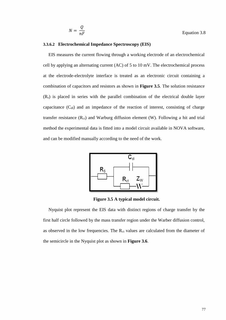
77
𝑁 = 𝑄
𝑛𝐹
Equation 3.8
3.3.6.2 Electrochemical Impedance Spectroscopy (EIS)
EIS measures the current flowing through a working electrode of an electrochemical
cell by applying an alternating current (AC) of 5 to 10 mV. The electrochemical process
at the electrode-electrolyte interface is treated as an electronic circuit containing a
combination of capacitors and resistors as shown in Figure 3.5. The solution resistance
(Rs) is placed in series with the parallel combination of the electrical double layer
capacitance (Cdl) and an impedance of the reaction of interest, consisting of charge
transfer resistance (Rct) and Warburg diffusion element (W). Following a hit and trial
method the experimental data is fitted into a model circuit available in NOVA software,
and can be modified manually according to the need of the work.
Figure 3.5 A typical model circuit.
Nyquist plot represent the EIS data with distinct regions of charge transfer by the
first half circle followed by the mass transfer region under the Warber diffusion control,
as observed in the low frequencies. The Rct values are calculated from the diameter of
the semicircle in the Nyquist plot as shown in Figure 3.6.

78
Figure 3.6 Model fit in Nyquist plot.
3.4 Nano-ferrites applications
Nanoferrites are made for a variety of purposes and the purpose
characteristically edict the content and precursors.
3.4.1 Nano-ferrites
Sample preparation is a critical step before physic-chemical analysis. The
target molecules are usually present at very low concentration while interfering
substances are usually present at higher concentrations. The quality of samples is
ensured by taking different replicates samples from each bulk. Therefore, the target
molecules need to be enriched; at the same time, the interfering substances need to be
removed. A variety of functionalized materials such as activated carbons, silica,
polymeric materials, nanoparticles, ferrites and biomass derived adsorbents have been
used for the selective capture and enrichment of samples. Sample enrichment units
are fabricated using these materials to suit the analysis needs of particular sample.
3.4.2 Analysis techniques
The heavy metals analysis procedure involve inductively coupled plasma
mass spectroscopic (ICP-MS) analysis for multiple metals analysis e.g. Ca, Mg, Pb,
As, and Cr. A high performance liquid chromatography (HPLC) method was
employed to separate and measure the amount of organic pollutant acephate. The
amounts of anionic species e.g. F-, Cl-, NO3- and SO4
2- were estimated by ion

79
chromatography.
3.5 Modelling adsorption
3.5.1 Response Surface Model
The statistical models i.e. response surface standard method of experimental
design was followed to study the effect of linear, interaction and quadratic effects of
experimental factors. According to the selected DOE method, a central composite
design (CCD) option was chosen in the Stat Ease 9.0 software. The modelling of
adsorption process was carried out based on the designed experiments by the software
to study the individual as well as the group effects of the factors selected for the
present study. The experiments were repeated to determine any systematic or
nonsystematic errors of the present adsorption system. The adsorbent adsorption
capacity (Qe mg.g-1) was calculated by Equation 3.9 (Shanmugaprakash et al., 2013).
𝑄𝑒 =(𝐶𝑜−𝐶𝑒)𝑉
𝑚 Equation 3.9
Where, Co and Ce stand for initial and equilibrium adsorbate concentration
(mgL-1) respectively, V is the total volume of solution in liters and m is the mass of
adsorbent (g). Adsorption experiments were repeated to check for systematic
variations to determine standard deviation and reproducibility of results. Four
variables are Adsorbate initial conc. (mgL-1), pH, temp and Adsorbent (Ads. mg) in
the range of 300-500 mgL-1, 3.0 to 9.0, 20 to 40 and 400 to 600 (mg) respectively. In
this work, equation 3.10 is used for the selected quadratic model (ZHANG ET AL.,
2015).
𝑸𝒆 = 𝜷𝒐 + ∑ 𝜷𝒊𝒙𝒊
𝒌
𝒊=𝟏
+ ∑ 𝜷𝒊𝒙𝒊𝟐
𝒌
𝒊=𝟏
+ ∑ ∑ 𝜷𝒊𝒋
𝒌
𝒋=𝟐
𝒙𝒊
𝒌−𝟏
𝒊=𝟏
𝒙𝒋 + 𝜺 𝒊 ≠ 𝒋 Equation
3.10
[Where βo is a constant coefficient, ε represents error, xi and xj are
80
independent variables, βi, βii and βij represent coefficients of linear, quadratic and
interaction effects respectively. The adsorption data of each experiment were
analyzed and fitted into the quadratic models. The models were verified by statistical
tests i.e. analysis of variance (ANOVA), residuals analysis (RA), scaling residuals
(SR) and prediction error sum of squares (PRESS) (Naseri et al., 2014). The verified
and validated models were applied to optimize the four input variables and to
maximize output i.e. fluoride, nitrates, nitrites, sulphates, phosphates, arsenic,
cadmium, nickel, iron and related heavy metals adsorption capacity.]
3.5.2 Isotherms
Adsorbate-adsorbent interaction can also be presented in the form of
isotherm, by plotting of the equilibrium concentration of ions in the exchanger or the
solid phase versus equilibrium concentrations of the same ions in the co-existing
solution phase. The design of hydro-decontamination system requires a thorough
analysis of the adsorption capacity (Qe) of each adsorbent and the percent removal
(%R) efficiency. The adsorption process is taken to be completed in four steps i.e.
bulk diffusion, film diffusion, pore diffusion and chemical reaction. First, the sorbate
molecules travel from the solution to the sorbent surface where they diffuse through
the boundary layer to the surface of the material. Then, these sorbate molecules
diffuse into the interior of the particles where they chemically react with active sites
on the surface of the sorbent. To verify the physical adsorption in the sorbent network
and chemical interaction in the dye molecules during the adsorption process, several
equilibrium models have been known to be used (Kyzas et al., 2015; Kyzas et al.,
2015; Świetlik et al., 2015). The basic purpose of these equilibrium isotherms is to
provide an insight into the molecular interaction. The suitability of a particular
isotherm is decided based on the correlation coefficient (R2) which is ideally 1, while

81
the other parameter is the degree of agreement between the experimental results and
the isotherms predicted results. These parameters help to assess and decide on the
success rate of a particular hydro-decontamination system and on the viability of the
process for a specific contaminant at certain geological locations.
3.5.2.1 Langmuir Isotherm for monolayer adsorption
This model assumes an ideal localized monolayer adsorption phenomena on
the surface of adsorbents. Each adsorbent has a fixed number of sites while each site
can adsorb only one adsorbate ion or molecule. As all sites are uniform so the energy
of adsorption is the same throughout the adsorbent surface. The linear Langmuir
adsorption model (Gimbert et al., 2008), is given as equation 3.11.
𝐶𝑒
𝑄𝑒=
1
𝐾𝐿+ 𝑎𝐿
𝐶𝑒
𝐾𝐿 Equation 3.11
The Langmuir constants, KL and aL are related to the adsorption energy and
the binding force between adsorbent and adsorbate. The maximum adsorption
capacity (Qm) can be calculated from the ratio of these constants. The maximum
adsorption capacity (Qmax) Equation 3.12.
𝑄𝑚𝑎𝑥 =𝐾𝐿
𝑎𝐿 Equation 3.12.
The dimensionless separation factor (RL) Equation 3.13, explains the nature of
adsorption process. It can be calculated using:The separation factor.
𝑅𝐿 = 1
1 + 𝐾𝐿𝐶𝑒 Equation 3.13.
When RL equals to zero it means irreversible adsorption process, a value from zero to
one indicates favorable adsorption, while a value of more than one represents

82
unfavorable process.
3.5.2.2 Freundlich isotherm for heterogeneous adsorption
The Freundlich model explains the heterogeneous adsorption process at the
adsorbate-adsorbent interface showing multilayer adsorption. Multiple adsorption is
characteristic of adsorbents with affinities for the toxic substances due to their better
surface morphology, porous structure and range of surface functional groups. This
model assumes exponential distribution of surface active sites and energetics of
adsorption systems. The primary adsorption sites are occupied first by the adsorbate
molecules that forms a layer on which the secondary or tertiary layers of adsorbate
are formed. However, the limitation of this model is that as the number of layers
increases the adsorption desorption phenomenon takes place in these systems. The
Freundlich model (Crini et al., 2007) is illustrated as Equation 3.14.
𝑙𝑛𝑞𝑒 = 𝑙𝑛𝐾𝐹 +1
𝑛 𝑙𝑛𝐶𝑒 Equation3.14.
Where, qe, is the equilibrium amount of adsorbate (mg g-1); KF, the Freundlich
constant associated with the degree of adsorption; 1/n, the heterogeneous factor
related to the intensity of adsorption. A value of 1/n greater than unity represents the
physical adsorption.
3.5.2.3 Temkin Isotherm for energetics of adsorption
Temkin isotherm assumes that the heat of the adsorption process for all the
molecules present in an adsorbed layer decreases linearly with surface coverage. It
helps to calculate the energetics of the system and provides an insight on the
exothermic and endothermic nature of the adsorption process. It can also be used to
calculate the free energy of the system, entropy and enthalpy of the system.

83
According to the Temkin model, adsorption is characterized by a uniform distribution
of binding energies up to some maximum value. The linear form of this model is
given as Equation 3.15:
𝑞𝑒 = 𝐵𝑡𝑙𝑛 𝐾𝑇 + 𝐵𝑡 𝑙𝑛𝐶𝑒 Equation 3.15
Where KT is the equilibrium binding constant corresponding to the
maximum binding energy, and Bt = RT/B is related to the heat of adsorption. The
value of KT and Bt are obtained from the intercept and slope of the plot of qe versus ln
Ce respectively.
3.5.2.4 Flory Huggin (FH) model for degree of surface coverage
The FH model accounts for the degree of surface coverage that is
characteristic of adsorbate and adsorbent. The linear form of the FH equation is
represented by:
𝑙𝑜𝑔𝑄
𝐶𝑖= 𝑙𝑜𝑔𝐾𝐹𝐻 + 𝑛 log(1 − 𝑄) Equation 3.16
Where Q is the degree of surface coverage, which can be calculated by the following:
𝑄 = 1 −𝐶𝑒
𝐶𝑖 Equation 3.17
Where n is the number of adsorbate molecules occupying the adsorption sites, KFH is
the equilibrium constant. The n and KFH constants can be calculated from the slope
and intercept of the curve log Q/Ci versus log (1-Q).
3.5.2.5 Dubinin-Radushkevich (D-R) isotherm
The linear form of Dubinin Rudushkevish (Dubinin et al., 1947) model is
given as Equation 3.18.

84
𝑙𝑛𝑄𝑒 = 𝑙𝑛𝑋𝑚 − 𝐾𝐷𝑅𝜀2 Equation 3.18
The value of Xm represents the monolayer sorption capacity (mg g-1); it can be
calculated from the intercept of the plot between ln Qe and ε2.
Equation 3.19: DR model ε.
𝜀 = 𝑅𝑇𝑙𝑛 (1 +1
𝐶𝑒 ) Equation 3.19
3.5.3 Adsorption Kinetics
For the design of an effective hydro-decontamination system we need to
know the rate of chemical reaction taking place i.e. the rate of adsorption. With
reference to geochemical modelling, we do not attempt to explain in detail the broad
field of chemical kinetics, but just enough to understand the basics of kinetics.
Several kinetic models are implemented to examine the experimental data to decide
on the nature, intensity and mechanism of the adsorption process. The speed of
adsorption was evaluated by employing four kinetic models: pseudo-first order,
pseudo-second order, intraparticle diffusion and Banghams. The overall adsorption
rate is proportional to the driving force and the concentration gradient in the case of
the first order, while in the case of the second order, it is proportional to the square of
driving force.
3.5.3.1 Rate law
A rate law is a statement about how the rate of a reaction depends on the
concentration of the participating species (Reactants). If we think at the molecular
level, imagine molecules colliding with one another. The overall reaction rate is
controlled by the number and orientation of collisions and the number and type of

85
molecules interacting. Let say we have a general reaction as in Equation 3.20.
aA + bB--cC + dD Equation 3.20
Where A, B, C and D are the chemical formulae, and a, b, c and d are the
stoichiometric coefficients. The rate of reaction can be written as Equation 3.21:
𝑅 = 𝑑𝜉
𝑑𝑡𝑘. 𝐶𝐴
𝑛𝐴𝐶𝐵𝑛𝐵𝐶𝐶
𝑛𝐶𝐷𝐷𝑛𝐷
Equation 3.21
The variable ξ is called the reaction progress variable and the
proportionality constant, k, is called the rate constant. The exponents nA, nB,…. .nD
are either integers or decimals and are used to calculate the order of a reaction. If nA
is 1, the reaction is designated as first order and if 2 as second order. The sum of
exponents gives the overall order of the reaction. Rate laws are determined by
analyzing one or more reactant or product as a functional of time as the reaction
proceeds, and then fitting the results to see what theoretical model fits the data.
3.5.3.2 Zero order
A reaction is zero order if the rate of reaction is independent of substrate
concentration, so the rate of reaction is constant. A plot of concentration vs. time will
thus give a straight line. For example, bacterial reduction of sulfate in marine
environments, where variables other than sulfate are constant (Gattuso et al., 1998).
Equation 3.22. Zero order
−𝑑𝐶
𝑑𝑡= 𝑘 Or Ct= Ci-k.t Equation 3.22
Where Ci and Ct are the reactants concentration at t= 0 and t=t respectively.

86
3.5.3.3 First order
A first order reaction proceeds at a rate that depends only on the
concentration of A as shown below. The more quantity of the reactant A, the more
product is formed and vice versa.
A Products
For example, the burning of methane in the air will continue only for as long
as it is available. If all exponents in Equation 3.22, are zero except of nA =1, then the
rate law becomes:
𝑑𝜉
𝑑𝑡=
𝑑𝐶𝐴
𝑑𝑡= 𝑘. 𝐶𝐴 Equation 3.23
For example, decay of radioactive elements is a first order reaction. Suppose CA = C
and C= Co, when t=0, then Equation 3.20, can also be simplified in the following forms
(Zhu et al., 2002).
Equation 3.24
These forms show the various ways to plot data to see if they fit first order rate law.
For example, a plot of ln (Co/C) vs. t will contribute a straight line with a slope equals to
the rate constant for change in reactants concentration.
3.5.3.4 Second order
The bimolecular collisions reaction are generally second order. For example:
A+B Products

87
The rate law is proportional to the concentration of the reactants and the
concentration of products has no effect on the rate of reaction. There are a number of
other rate laws, but this will suffice to give an idea of the procedures. However, due to
the complexity of chemical reactions, understanding them in terms of their fundamental
mechanisms is not easy to achieve.
3.5.3.5 Pseudo order reactions
In the natural environment, we observe complex reactions that are not zero, first or
second order but they partially follow the order criteria and are named as pseudo order
reactions. Let us consider a reaction where A and B react to form a product (P).
A+B P
The rate equation for this general reaction can be written as Equation 3.25.
Rate = k. [A]1[B]1 (Overall order = 2) Equation 3.25
Now suppose we perform an experiment in which [A] = 0.01 mol dm-3 and [B] =
0.100 mol dm-3, i.e. B is 10 times more concentrated. After completion of the reaction,
the concentration of reactant B remaining will be [B] = 0.099 ~ 0.100 mol dm-3 i.e. the
concentration of B remains unchanged.
For experiments where [B]>>[A], or [B] = constant, Equation 3.25 becomes:
Rate= k. [A]1[B]0 or Rate= k. [A]1
The experimental results show that the reaction is first order instead of second order as
determined by chemical equation. Such type of reaction in which a reactant is much
more concentrated than the other, the concentrated reactant is made to have no effect on
the rate law, resulting in an overall pseudo order reactions.

88
3.5.3.6 Pseudo-First Order Kinetic Model
The pseudo-first order kinetic model is widely used to predict the adsorption
mechanism. The linear form of the pseudo-first order model is given by Equation
3.26.
ln( 𝑞𝑒 − 𝑞𝑡) = 𝑙𝑛 𝑞𝑒 − 𝑘1𝑡 Equation 3.26
Where k1, is the first-order rate constant of adsorption, while qe and qt are
the maximum amount adsorbed at equilibrium and at time t, respectively. The linear
plots of ln(qe –qt) versus t yield straight lines. The values of k1 (min-1) and qe (mg g-1)
can be calculated from the slope and intercept of the pseudo first order linear plots.
3.5.3.7 Pseudo second order model
The linear form of the pseudo-second-order model is given by Equation
3.27:
𝑡
𝑞𝑡=
1
𝑘2𝑞𝑒2
+ 𝑡
𝑞𝑒 Equation 3.27
Where k2 (g mg-1 min-1) is the rate constant of pseudo-second order kinetic equation,
which can be calculated from the intercept of the linear plot of time versus t/qt. The
equilibrium adsorption capacity (qe) can be calculated from the slope.
3.5.3.8 Intraparticle Diffusion Model
The intraparticle diffusion model was used to evaluate the experimental data
to see the possibility of intraparticle diffusion as the rate limiting step. It is given as:
Equation 3.28: Intra-particle diffusion model.
𝑞𝑡 = 𝑘𝑖𝑑𝑡12
+ 𝐼 Equation 3.28

89
Where kid (mg g-1 min-1/2) is the intra-particle diffusion rate constant and I is the
boundary layer effect (mg g-1). The value of I is directly proportional to the boundary
layer thickness. According to Equation 3.28, the plot of qt versus t1/2 should be a
straight line with a slope Kid and intercept I when the mechanisms follow the intra-
particle diffusion model.
3.5.3.9 Banghams’s Model
The hydro-decontamination kinetic data was evaluated with Banghams’s
equation (Equation 3.29) to determine the slowest or the rate-controlling step during
the adsorption process.
log (𝑙𝑜𝑔 (𝐶𝑂
𝐶𝑂 − 𝑞𝑡𝑚)) = log (
𝑘𝑜𝑚
2.303 𝑉) + 𝛼 log(𝑡) Equation 3.29
Where V is the volume of solution (l) and α and ko are constants.
3.5.4 Thermodynamics
The study of adsorption reaction dependent on temperature gives valuable
information about the change in free energy, enthalpy and entropy during adsorption.
The values of adsorption energies (∆G, ∆H and ∆S) are calculated using the following
equations.
∆𝐺 = −𝑅𝑇 𝑙𝑛 𝐾𝐿 Equation 3.30
ln𝐾2
𝐾1= −
∆𝐻
𝑅 (1𝑇2
−1𝑇1
)
Equation 3.31
∆𝐺 = ∆𝐻 − 𝑇∆𝑆 Equation 3.32

90
CHAPTER 4: RESULTS AND DISCUSSIONS
This chapter describes the results and discussion related to the main phases of this
study. In the phase I, adsorbent characterization results are discussed. While in the
phase II, application and modelling results are presented. The following sub-section
describes the characterization of adsorbents, followed by application for green
environment remediation.
4.1 Characterization results of CuCe0.2Fe1.8O4-rGO.
The characterization of adsorbents is an important step in the exploration of surface
active functional groups, shape and size of particles, phase purity, optical band gap and
chemical composition. In the present work, the synthesized adsorbents were
characterized by different spectroscopic and analytical techniques. “The crystal
structure, crystallite size and lattice strain of the CuFe2O4, CuCe0.2Fe1.8O4 ferrite
nanoparticles, and graphene-based CuCe0.2Fe1.8O4 nanocomposites were observed by an
X-ray diffractometer (XRD, PANalytical Empyrean), equipped with a monochromatic
Cu Kα radiation source. Fourier transform infrared spectroscopy (FTIR) was carried out
on a Perkin Elmer System 2000 series spectrophotometer (USA) between 4000-400 cm-
1. Thermogravimetric analysis (TGA) was used to examine the graphene and graphene-
based CuCe0.2Fe1.8O4 nanocomposites. Energy dispersion spectroscopy (EDS),
elemental mapping, and Field Emission Scanning Electron Microscopy (FESEM) were
applied to study the elemental composition, the surface distribution of the elemental
components, and particle size and distribution. Raman spectroscopy, (Renishaw 2000
system) was performed using a green laser operating at 532 nm and room temperature.
The magnetic hysteresis loops of CuFe2O4, CuCe0.2Fe1.8O4, and graphene-based
CuCe0.2Fe1.8O4 nanocomposites were recorded on a Vibrating Sample Magnetometer
(VSM).”

91
4.1.1 XRD analysis
Figure 4.1 shows the XRD patterns of the CuFe2O4, CuCe0.2Fe1.8O4 ferrite
nanoparticles, and graphene-based CuCe0.2Fe1.8O4 nanocomposites. We observed the
single-phase structure of CuFe2O4 that was obtained at 800oC and was indexed using
JCPDS#034-425. Figure 4.1 (b) displays the diffraction patterns of the CuCe0.2Fe1.8O4
ferrite nanoparticles. The structure shows the major peak (311), while two other peaks
represent the CeO2 peaks, and was indexed using JCPDS#043-1002 (Fig. 2b). The
second phases were observed by adding Ce3+ content into the CuFe2O4 ferrite. However,
by increasing the Ce3+(x>0.2), more peaks of CeO2 and Ce2O3 can be seen, which may
be the result of the larger ionic radii of Ce3+(1.020Å ) as compared to Fe3+ (0.645 Å)
(Wu et al., 2014). Thereby, we have investigated the second phase in the CuCe0.2Fe1.8O4
spinel ferrite structure. After the addition of graphene, similar developments were
observed when looking at CuCe0.2Fe1.8O4. In fact, due to the inherent low crystalline
structure of graphene, the typical peaks of graphene were absent in the XRD patterns
(Figure 4.1 (c)). However, a slight increase in the peak increases with the introduction
of graphene, which was noticed with the crystallite refinement and lattice microstrain
decrement. During the formation of the CuCe0.2Fe1.8O4 spinel ferrite structure, Ce3+ ions
were dissolved in the medium to form a solid solution. Annealing at 800oC, this forced
the Ce3+ ions to migrate into the crystal structure, spaces or grain boundary sites. The
large ionic radius of Ce3+, as compared to Fe3+(Wu et al., 2014), offered a relative space
interference to viable vacant crystal or interstitial sites in copper ferrites. Consequently,
the excess Ce3+ ions oxidized into Ce4+ at this temperature and appeared as a separate
phase in the XRD spectra.
XRD scientists have developed various theoretical models to assess these structural
features through the mathematical analysis of XRD patterns. In this study, the average
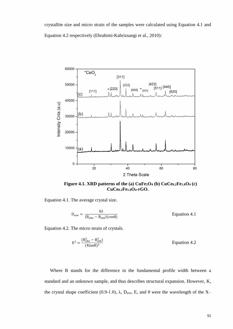
92
crystallite size and micro strain of the samples were calculated using Equation 4.1 and
Equation 4.2 respectively (Ebrahimi-Kahrizsangi et al., 2010):
Figure 4.1. XRD patterns of the (a) CuFe2O4 (b) CuCe0.2Fe1.8O4 (c)
CuCe0.2Fe1.8O4-rGO.
Equation 4.1. The average crystal size.
Dave = kλ
(Bobs − Bstd)(cosθ) Equation 4.1
Equation 4.2. The micro strain of crystals.
E2 =(Bobs
2 − Bstd2 )
(4tanθ)2 Equation 4.2
Where B stands for the difference in the fundamental profile width between a
standard and an unknown sample, and thus describes structural expansion. However, K,
the crystal shape coefficient (0.9-1.0), λ, Dave, E, and θ were the wavelength of the X–

93
ray (0.15406 nm), average crystallite size, mean lattice distortion (lattice strain), and
Bragg’s angle (°) respectively.
Table 4.1. Crystallite sizes and micro-strain in CuFe2O4, CuCe0.2Fe1.8O4, and
graphene CuCe0.2Fe1.8O4 nanocomposites.
Ferrites Crystallite size (D nm) Lattice strain (η,%)
CuFe2O4 28±2.1 0.424±0.021
CuCe0.2Fe1.8O4 50±1.3 0.251±0.017
CuCe0.2Fe1.8O4-rGO 59±1.7 0.211±0.019
The important features of CuFe2O4 and CuCe0.2Fe1.8O4 spinel ferrites in the presence
and absence of graphene were compared (Table 4.1). In this case, CuFe2O4 ferrite has a
crystallite size of 28±2.1nm and a lattice micro strain of 0.424±0.021. In the absence of
rGO, the average crystallite size of the CuCe0.2Fe1.8O4 was 50.5±1.3nm and the lattice
micro strain was 0.251±0.017. However, with the creation of rGO, we observed a slight
increase in the average crystallite size (59.3±1.3 nm) and lattice micro strain
(0.211±0.019). We noticed that the crystallite size increased with the introduction of
both Ce3+ matter and rGO. We furthermore observed that the combination of rare earth
ions and graphene with a CuFe2O4 spinel structure would also affect the physical forms,
functional groups, morphologies and magnetic properties.
4.1.2 FTIR functional groups
Figure 4.2 details the comparative FTIR functional groups of the CuFe2O4,
CuCe0.2Fe1.8O4 ferrite nanoparticles and graphene-based CuCe0.2Fe1.8O4
nanocomposites. Fig. 3a displays the distinguishing absorption peaks of a typical
CuFe2O4 ferrite (Rehman et al., 2015). Fig. 3b shows the depletion of 3360 cm-1 bands,
while the appearance of 1470 cm-1 clearly indicates the creation of CuCe0.2Fe1.8O4. The
involvement of CuFe2O4 functional groups with the arriving Ce is seen in the complete
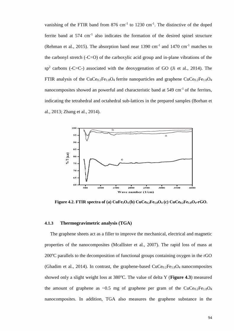
94
vanishing of the FTIR band from 876 cm-1 to 1230 cm-1. The distinctive of the doped
ferrite band at 574 cm-1 also indicates the formation of the desired spinel structure
(Rehman et al., 2015). The absorption band near 1390 cm-1 and 1470 cm-1 matches to
the carbonyl stretch (-C=O) of the carboxylic acid group and in-plane vibrations of the
sp2 carbons (-C=C-) associated with the deoxygenation of GO (Ji et al., 2014). The
FTIR analysis of the CuCe0.2Fe1.8O4 ferrite nanoparticles and graphene CuCe0.2Fe1.8O4
nanocomposites showed an powerful and characteristic band at 549 cm-1 of the ferrites,
indicating the tetrahedral and octahedral sub-lattices in the prepared samples (Borhan et
al., 2013; Zhang et al., 2014).
Figure 4.2. FTIR spectra of (a) CuFe2O4 (b) CuCe0.2Fe1.8O4 (c) CuCe0.2Fe1.8O4-rGO.
4.1.3 Thermogravimetric analysis (TGA)
The graphene sheets act as a filler to improve the mechanical, electrical and magnetic
properties of the nanocomposites (Mcallister et al., 2007). The rapid loss of mass at
200oC parallels to the decomposition of functional groups containing oxygen in the rGO
(Ghadim et al., 2014). In contrast, the graphene-based CuCe0.2Fe1.8O4 nanocomposites
showed only a slight weight loss at 380oC. The value of delta Y (Figure 4.3) measured
the amount of graphene as ~0.5 mg of graphene per gram of the CuCe0.2Fe1.8O4
nanocomposites. In addition, TGA also measures the graphene substance in the

95
nanocomposites. We noted that the rGO decomposition peak was absent and that the
decomposition of the graphene-based CuCe0.2Fe1.8O4 nanocomposites shifted to a higher
temperature (380oC). This indicates the structural strength of the nanocomposites, which
may be due to the incorporation of graphene and the forerunner CuCe0.2Fe1.8O4.
Figure 4.3. TGA analysis of (a) rGO (b) CuCe0.2Fe1.8O4-rGO nanocomposites.
4.1.4 Morphology and microstructural analysis
The Figure 4.4 shows FESEM images of graphene, CuFe2O4, CuCe0.2Fe1.8O4, ferrite
nanoparticles and graphene-based CuCe0.2Fe1.8O4 nanocomposites. Fig. 5a demonstrates
the agglomerated CuFe2O4 nanoparticles. However, the CuCe0.2Fe1.8O4 ferrite
nanoparticles have less agglomeration as compared with CuFe2O4, which may be the
result of additional Ce3+ content. This change in behavior is credited to the van der
Waals interactions seen in the specific large surfaces of the fine particles. From a
nanochemistry point of view, neighboring nanoparticles sharing a common

96
crystallographic orientation may collide with each other, which produces coalescence
(Balaz, 2008). Therefore, the adjacent primary particles appear to aggregate, yielding
larger secondary particles. In addition, owing to their nanometer size, the nanoparticles
collide and coalesce in a fashion that again results in bigger particles. This phenomenon
may eventually cause agglomeration in the fabricated samples. In agreement with Fig.
5b, the average size of the inter- and intra-agglomerate pores were 300 and 30 nm,
respectively.
Figure 4.4. FESEM images (a) CuFe2O4 (b) CuCe0.2Fe1.8O4 (c) CuCe0.2Fe1.8O4-
rGO nanocomposites.
It is clear that the intra-agglomerate pore sizes are relatively smaller than the inter-
agglomerate pore sizes. On the other hand, in the presence of graphene, the
CuCe0.2Fe1.8O4 nanoparticles were adsorbed on the graphene sheets in the synthetic
process (Fig. 5c). Similar to the CuCe0.2Fe1.8O4 nanoparticles, the graphene-based
CuCe0.2Fe1.8O4 nanocomposites indicated a high tendency to agglomerate (Fig. 5d). The
various processing parameters, such as the mixing speeds, intensity, and time, affected

97
the extent of agglomeration. Here, during co-precipitation and hydrothermal synthesis,
the rate of particle collision increased and the resultant particles aggregated into larger
particles. The average grain size of the CuCe0.2Fe1.8O4 nanoparticles was 43±2 nm. In
addition, the graphene sheets, with some wrinkles and folds, possessed a large aspect
ratio, which is the main factor behind the intensification of the contact area with the
ferrites phases.
4.1.5 EDS and elements maps
The EDS study and the relative distribution of the constituent elements provided
exemplification of the XRD results, as shown in Fig. 6. The percentage (%) of the
individual elements in the present composite was: 36.72, 29.49, 17.86, 12.30, and 3.63,
of Fe, O, Cu, Ce and C respectively. We observed the carbon peak with a relative
percentage of elements in the EDS full-scale profile of the sample. Interestingly, the
EDS results show carbon peaks that were not prominent in the XRD spectrum (Figure
4.5). The EDS results also disclose nonappearance of any impurities during the followed
synthesis route.
Figure 4.5. EDS and elemental mapping in CuCe0.2Fe1.8O4-rGO nanocomposites.
The elemental mapping shows a uniform distribution of the constituent elements
carbon, copper, cerium, oxygen, and iron all over the nanocomposites (Fig. 6). The

98
results confirmed the formation of the graphene ferrite’s uniform microstructure through
the hydrothermal process.
4.1.6 Raman Spectroscopy
The Raman spectroscopy, a powerful analysis tool is used to distinguish between the
GO and rGO (Mondal et al., 2015; Wu et al., 2009; Zhang et al., 2014). Raman is a non-
destructive structural scrutinizing tool for the analysis of graphene based materials
(Ferrari et al., 2006; Meidanchi et al., 2014). The precursor graphite shows in phase
vibrations because of the highly ordered graphaite lattice (G band) and disorder graphite
edges (D band) at 1575 cm-1 and 1355 cm-1 respectively (Figure 4.6) (Calizo et al.,
2007; Ferrari et al., 2006). The D band is credited to the lattice defect induced phonon,
and G band refers to the C-C bond increase or contraction in the hexagonal carbon
conformations (Shahid et al., 2014; Shahid et al., 2015). In contrast, the GO and rGO
has well defined D and G bands near 1343 cm-1 and 1596 cm-1 (Kudin et al., 2008). A
small bump in Raman spectrum near 2685 cm-1 allotted to the 2D band in rGO
associated with the reduced number of re-stacking because of the incorporation of
ferrites during the hydrothermal process (Akhavan, 2015). The 2D band also suggest the
construction of exfoliated rGO sheets from the dense multilayer GO (Calizo et al.,
2007). It is also because of the spacer role of the Nano ferrites as confirmed by the
FESEM. The Raman shift of G band of rGO also demonstrates the “self-healing”
properties of the rGO (Cui et al., 2015). These observations support the successful
transformation of Go to rGO during the hydrothermal process. Moreover the intensity
ratio of the D to G band (ID/IG) is another Raman parameter that is related with the
degree of disorder and interatomic size of the Sp2 hybridized carbons (Meidanchi et al.,
2014; Shahid et al., 2015). The ID/IG ratio for rGO (1.064) is higher than GO (0.88),
suggesting the formation of partially ordered crystal structures and relatively stronger
bonding (Bacsa et al., 2015) . The Raman spectroscopic analysis results also

99
complements the thermal analysis (TGA & DTA) associated to the relative stability of
the nanocomposites because of the additional π bonding stability in the doubly bonded
carbons in rGO (Chia et al., 2015).
Figure 4.6. Raman spectrum of CuCe0.2Fe1.8O4-rGO nanocomposites.
4.1.7 Magnetic hysteresis loops
Figure 4.7(a-c) shows the hysteresis loops of the CuFe2O4, graphene-based
CuCe0.2Fe1.8O4 nanocomposites, and CuCe0.2Fe1.8O4 nanoparticles, which were
measured at room temperature (25 ±0.6oC) with a maximum applied field from -12000
to 12000 Oe. The hysteresis loops revealed the magnetic properties, such as saturation,
magnetization, remanence and coercive force, of the prepared samples. We observed
that the CuCe0.2Fe1.8O4 nanoparticles demonstrated an increase in magnetic remanence
(Mr), as compared with the CuFe2O4 and graphene-based CuCe0.2Fe1.8O4
nanocomposites. The CuCe0.2Fe1.8O4 nanoparticles show a relatively large magnetic
saturation (Ms). The intrinsic and extrinsic factors contributed to the noteworthy
improvements in both Mr and Ms in the presence of Ce3+ and graphene. The extrinsic
factors depend on the morphology, density, and grain size of the nanoparticles (Potts et

100
al., 2011), whereas the intrinsic factors, such as the relative occupation of the sub-lattice
sites, contributed to the magnetism in the Nano ferrites (Raju et al., 2014). The shape
and width of the hysteresis loops depends on the method of preparation, composition,
and the spreading of metals cations at the tetrahedral and octahedral sites, in addition to
the spin canting and crystallite size (Borhan et al., 2013). The synthesis processes for
the nanocomposites were the same, however, the incorporation of graphene in the
CuCe0.2Fe1.8O4 nanocomposites increased the tetrahedral and octahedral distribution of
the metal cations, changed the surface morphology, and decreased the crystal strains
(Rehman et al., 2015). Consequently, these magnetic properties revealed a remarkable
improvement in the nanocomposites, which could be attributed to the presence of Ce3+
and rGO. It must be added that a variation in the coercive field (Hc) directly depended
on the surface spin disorder (Kostopoulou et al., 2014). The FESEM images illustrated
the homogenous distribution of the CuCe0.2Fe1.8O4 nanoparticles over the graphene
sheets, which in turn revealed that inactive magnetic behavior reduces magnetization.
Therefore, the saturation and remanence decreased when compared to the
CuCe0.2Fe1.8O4 nanoparticles. The decrease in Hc for the graphene-based CuCe0.2Fe1.8O4
nanocomposites confirmed that rGO reduced the surface spin disorder.
Table 4.2 lists the squareness ratio (Mr/Ms) of the individual ferrite samples. The
squareness ratio increased after the combination of Ce3+ in the CuFe2O4, whereas it
decreased with the supplement of graphene in the CuCe0.2Fe1.8O4.
Table 4.2. Magnetic saturation (Ms), remanence (Mr) and coercivity (Hc) of
CuFe2O4, CuCe0.2Fe1.8O4 and graphene - CuCe0.2Fe1.8O4.
Ferrites Hc (Oe) Mr (emu/g) Ms (emu/g) Mr /Ms
CuFe2O4 1044 11.38 15.53 0.73
CuCe0.2Fe1.8O4 690 24.41 30.13 0.81
CuCe0.2Fe1.8O4-rGO 910 19.96 25.32 0.79

101
Figure 4.7. VSM hysteresis loops of (a) CuFe2O4 (b) CuCe0.2Fe1.8O4-rGO (c)
CuCe0.2Fe1.8O4 nanocomposites.
“The decreasing behavior of the coercivity shows an improvement in the soft
magnetic character of the nanocomposites. The magnetic properties of the
CuCe0.2Fe1.8O4 ferrites were controlled by the Fe3+-Fe3+ interaction and spin coupling of
3d valance electrons (Dixit et al., 2012).” It was noted that the incorporation of
graphene in the CuCe0.2Fe1.8O4 improved the magneto-static interactions (Domingo et
al., 2012). The magnetic squareness ratio was less than one (>1), indicating the
paramagnetic characters of the prepared nanocomposites.
“In this study, the CuCe0.2Fe1.8O4 ferrite nanoparticles and the CuCe0.2Fe1.8O4
nanocomposites with graphene showed higher magnetic saturation levels and lower
levels of coercivity as compared to the original CuFe2O4 ferrite. This may be because of
the better morphology, increased magnetic moments, and domain wall migration of the
CuCe0.2Fe1.8O4/graphene nanocomposites (Dutta et al., 2006; Niaz Akhtar et al., 2014).
Furthermore, it was observed that the paramagnetic behavior of the Ce3+ ions would
102
lessen the resistance between the domain walls and weaken the exchange interactions,
which correspond to a decrease in the coercivity in the ferrites. Further study of the
VSM curves indicated a relatively Hc higher values as compared to magnetic ferrites
and magnetic saturation was less than 49 emu/g (Nguyen et al., 2014). A similar high
Hc (~1095 Oe) was found in the magnetic ferrites prepared by a micro-emulsion
method (Rashad et al., 2015). However, Rao et al. found relatively reduced Hc (575.2
Oe) but relatively lower Ms (10.47 emu/g) and Mr (5.38 emu/g) values for CuFe2O4 thin
films prepared by spray pyrolysis deposition technique (Rao et al., 2015). The magnetic
behavior can be explained on the grounds of the development of two independent
domains at tetrahedral and octahedral sites (A& B sites) that demonstrate ferromagnetic
nature through magnetic coupling interactions (Rao et al., 2015). A manganese
substituted ferrite (Mn-CuFe2O4) prepared by bio template medium and simple
evaporation method also exhibited comparable Hc (492 Oe) and Ms (10.42 emu/g)
(Ranjith Kumar et al., 2014). Based on these results, it is apparent that the
CuCe0.2Fe1.8O4 nanoparticles and CuCe0.2Fe1.8O4/graphene nanocomposites act as
potential candidates for superior catalysts, switching, electromagnetic wave absorbers
and adsorbents for environmental remediation.”
“Magnetic graphene nanocomposites were fruitfully prepared using a facile co-
precipitation hydrothermal reduction method. We assessed the structural,
morphological, thermal, and magnetic properties using XRD, FTIR, TGA, FESEM, and
VSM techniques, respectively. The magnetic Nano-composite showed improved
thermal stability, which can extend its application under more severe temperature
conditions. However, nanocomposites have a large crystallite size and large crystal
strains as compared to CuFe2O4 ferrites. The FESEM results indicate the distribution of
the CuCe0.2Fe1.8O4 ferrite constituent elements across the graphene surface. The
CuCe0.2Fe1.8O4-rGO magnetic nanocomposites demonstrated an improvement in its

103
magnetic, thermal and energy efficient separation properties. These improved magnetic
nanocomposites provide the basis for a broad range of applications and lead towards a
better understanding of energy storage, electromagnetic wave absorbers, chemical
process catalysts, electrochemical sensors and adsorbents for pollutants removal
technologies.”
4.2 Characterization results of Palm oil waste clinker sand.
The need of specific and competent adsorbents is increasing to remove heavy metals
or to maintain permissible levels in drinking water. The excellent experimental results
in comparison to external studies confirmed the relative importance of POCS based
arsenic removal system for a green environment remediation approach. The reuse or
recycle approach in industrial mega production industries is one of the most pertinent
desires to re-utilize the enormous volume of solid waste (Ahmad et al., 2011; Dias et al.,
2007; Hameed et al., 2009; Roig et al., 2006). Production managers always think about
alternative strategies to reuse waste by-products and accomplish goal of “zero waste”(Li
et al., 2007; Zaman et al., 2013). This is normally the case in palm oil industry in
Malaysia and neighboring countries, where oil palm shell and fibers is produced in large
amounts during oil extraction process (Ahmad et al., 2011). The generated waste left
after incineration of shell and fiber is researched for conversion into useful adsorbents.
At present. nearly 2.6 million tons of waste is a great challenge asking for reutilization
of waste resource along with environmental sustainability(Hameed et al., 2009).
Providentially, the industrial waste is recycled after suitable mechanical, chemical and
physical treatments. The recycle process helps in resources preservation, energy
efficient processing and environment friendly waste disposal (Ahmmad et al., 2014;
Hameed et al., 2009; Ryan et al., 2000).

104
4.2.1 POCS mechanical and physical treatments
The samples were grinded and forwarded to fractionation and separation process.
The US standard sieves of different pore sizes were used to makes different mechanical
grades. Each fraction was washed with distilled water to remove color and fine
particles. The POCS particles were dried in an electrical heating oven at ambient
temperature overnight. The fine grades were obtained after regrinding and sieving with
a 12.00-4.75 mm mesh size (Fig. 4.8).
Fig. 4.8. Mechanical and physical treatments.
4.2.2 Application of POCS for As adsorption
The adsorption experiments were planned to achieve maximum POCS adsorption
potential. Table 4.3 shows the factors names, codes and levels used to make design
matrix.

105
Table 4.3. The CCD variables, symbols and levels.
Variables Symbol Level
Low Mean High -α +α
POCS, mg X1 500 750 1000 250 1250
As, mg L-1 X2 100 175 250 25 325
T, oC X3 25 35 45 15 55
pH X4 4 6.5 9 15 115
The experimental data was collected as advised and designed by CCD, the
equilibrium arsenic concentration (Qe) was calculated by using equation 2.1
(Shanmugaprakash et al., 2013). The reproducibility of experimental adsorption
capacity was ascertained by repeating the experiments to account for standard deviation.
The applied method is robust and beneficial over the arsine gas generation method, as it
required no extra reagents to produce gaseous phase arsenic (arsine gas). The selected
quadratic model provided better insight into complex correlated, interacting adsorption
variables. It assisted to identify the most influencing as well as least influencing
variables (Roy et al., 2014). The interactive effects of four important variables were
discovered to describe the arsenic adsorption. The designated graphical models clearly
visualize and predict maximum arsenic adsorption. The value of each model coefficients
was expended to explain important relationships among independent and dependent
variables.
The experimental adsorption capacity was analyzed and model fitted to discover the
goodness of fit of the proposed model. Successively, model was tested by statistical
tests e.g. analysis of variance (ANOVA), residuals analysis (RA), scaling residuals (SR)
and prediction error sum of squares (PRESS) (Smith et al., 2000). The verified and
validated model was used to augment input process variables and to maximize output

106
i.e. arsenic adsorption. The decided statistical model was also validated by
supplementary experiments.
4.2.3 Batch adsorption
Arsenic adsorption study was performed in a batch mode of experiments. The pre-
weighted POCS (mg) was taken into the conical flask, 20 cm3 of analyte (As) of known
concentration was added and pH adjusted with drops of 0.01M HCl or 0.01M NaOH
respectively. Each sample flask was shaken (200 rpm) for 1 h, filtered through a PTFE
SIMPLEPURE (0.22 µm) micro filter, and collected into ICPMS ampoules for
subsequent analysis.
4.2.4 POCS Particle size distribution
Fig. 4.9 shows PSD curve correlating particle size with percent finer. It was observed
that POCS has a fitness modulus, specific gravity and water absorption of 3.09, 2.01
and 3.75 % respectively. These results indicated that POCS as a well graded material.
The PSD analysis was used to differentiate particle with appropriate features for arsenic
adsorption. Previously it was reported that the particle size has a direct effect on degree
of contact with desired adsorbate (arsenic) (Kim et al., 2013). The very fine particles
possess relatively large surface area and offer better contact with arsenic (Kim et al.,
2013). However, these very fine ultra-small particles were found to be unsuitable due to
difficult separation and blockage of filter during early viability studies. The small
diameter of particles offer extremely slows down speed of water molecules and causes
an impractical separation process. Accordingly, 600 µm particle size was selected for
further studies. The selected particles were found appropriate owing to porous
networking structures, specific gravity, fitness modulus and water absorption properties
(Ahmmad et al., 2014) .

107
4.2.5 Functional groups analysis
FTIR study provides useful functional groups information regarding arsenic and
POCS surface interactions during adsorption process. Surface interactions are due to
presence of surface functional groups.
Fig. 4.9. Particle size distribution curve of POCS.
The surface of POCS indicated a number of interesting functional group that possibly
become the reason for enhanced arsenic adsorption despite its porous networking
structures (Ferraro, 2012).
Figure 4.10 it can be seen that finger print region of IR spectrum contains a
dominant and distinct peaks at 1022 cm-1. It can be attributed to a number of
metals/nonmetals oxides generated during calcinations process in a boiler. Previous
studies observed a relative proportion of various metals, nonmetal and their respective
oxides (Ahmmad et al., 2014). These mixed oxides are responsible for improved arsenic
adsorption. A similar observations has been reported for a role of metal oxide for
interaction with arsenic during adsorption process (Ferraro, 2012). Due to abundant

108
oxides, peaks of other functional groups look weak and negligible at a first glance.
However, we selected a separate IR region from 1500 to 4000 cm-1 to account for other
functionalities, responsible for a higher arsenic uptake during current adsorption
process.
Figure 4.10 (insect)). Interestingly, the selected IR region shows peaks for other
functional groups for arsenic. Particularly, FTIR spectrum shows peaks at 518 cm-1 (C-
Br), 538cm-1(C-Cl), 621cm-1(N-H), 692 cm-1 (C-H), 710cm-1(C=C), 728-795 cm-
1aromatic (C=C), 800 cm-1 (C-H), 1022cm-1(C-N), 1056 cm-1 (Metal-O), 1160 cm-1
(C=O), 1426 cm-1 (C=C), 1623 cm-1 (C=N), 2106 (C≡ 𝑁), 2500-3000 cm-1 (C-H),
3176 cm-1 (N-H), 3219-3366 cm-1 (O-H). The functional groups study results verified
the role of multiple functional groups on adsorbent surface.
Figure 4.10. FTIR spectrum and functional groups peaks. Insect showing the
1200 to 4000 cm-1.

109
4.2.6 FESEM and EDX analysis
Figure 4.11 represents POCS surface morphology by FESEM. It can be seen that
there are pores of various sizes and diameters. Figure 4.11 (A) shows small scattered
fine particles and semi hexagonal type of pores on the porous networking surface. The
surface pore can be classified by further exploration of FESEM at different area into the
micrometer pores of small, medium and extra-large sizes (Figure 4.11 B & C). The
FESEM results visualize a heterogeneous adsorbent surface that is more suitable for
interactions and capture of arsenic. The elemental analysis of the selected area were
scanned and analyzed by energy dispersive X-rays (EDS). Figure 4.11 D provides the
relative percentage of elements e.g. silicon, oxygen, carbon, potassium, calcium,
magnesium, and aluminum 34.5, 31.6, 13.3, 12.6, 5.2, 2.1 and 0.8 weight %
respectively.
Figure 4.11. FESEMs, micro porous structure of POCS (A) 50 µm (B) 400 µm
(C 500 µm (D) EDX composition.

110
The FESEM surface and elemental analysis indicated that the indigenous POCS was
rich in a number of mixed metals, nonmetals and related oxides. Moreover, the
attractive functional groups like carbonyl (-C=O), cyano (-CN), hydroxyl (-OH) and
amide (-NH) groups (FTIR results) are very interesting for adsorption interactions.
4.2.7 A quantitative comparison of efficiencies
The adsorption capacities were compared and analyzed by an external comparative
study by comparing a number of adsorbents. For illustration, Ferrous ions laden Apricot
stone activated carbon (Qe= 5.91mg g-1) (Tuna et al., 2013.), Ferric ions and Apricot
stone activated carbon (Qe = 5.74mg g-1) (Tuna et al., 2013.), the mesoporous alumina
(Qe = 39.06 mg g-1) (Han et al., 2013), precipitated zeolites (ZNa-Fe) (Qe = 6.73mg g-
1) (Simsek et al., 2013), Aluminum(III) zeolites (ZNa-Al) (Qe = 3.79mg g-1) (Simsek et
al., 2013), and a thermally treated Iron on activated carbon (Qe = 4.56 mg g-1) (Nieto-
Delgado et al., 2012). It became clear through the present comparative study that POCS
has a better adsorption capacity. The relative measure of qe provides a basic scale to
recognize these new adsorbents and the prospective future application in adsorption
based remediation techniques.
4.3 Modelling adsorption.
The proposed model for arsenic adsorption by POCS is: Equation 4.3. The proposed
quadratic model for Arsenic.
𝑸𝒆 = +𝟏𝟓. 𝟖𝟐 + 𝟏. 𝟔𝟑 ∗ 𝑿𝟏 + 𝟏. 𝟖𝟒 ∗ 𝑿𝟐 + 𝟎. 𝟖𝟐 ∗ 𝑿𝟑 + 𝟑. 𝟏𝟐 ∗ 𝑿𝟒𝐗𝟒 + 𝟎. 𝟎𝟒 ∗𝑿𝟏 − 𝟎. 𝟏𝟕 ∗ 𝑿𝟏𝑿𝟑 + 𝟎. 𝟖𝟓𝑿𝟏𝑿𝟒 − 𝟎. 𝟐𝟓𝑿𝟐𝑿𝟑 − 𝟎. 𝟔𝟕 ∗ 𝑿𝟐𝑿𝟒 − 𝟎. 𝟑𝟒𝑿𝟑𝑿𝟒 −
𝟎. 𝟗𝟒 ∗ 𝑿𝟏𝟐 − 𝟏. 𝟎𝟑 ∗ 𝑿𝟐
𝟐 − 𝟎. 𝟓𝟕 ∗ 𝑿𝟑𝟐 − 𝟏. 𝟔𝟓 ∗ 𝑿𝟒
𝟐 Equation 4.3
Where the coded variables X1, X2, X3 and X4 represent POCS (mg), As (mgL-1),
Temp. (oC) and pH respectively. The influence of variables is sorted out by comparing
the coefficients obtained by the ANOVA test. The comparative values explain the
significance of respective variables. Generally, a positive regression coefficient
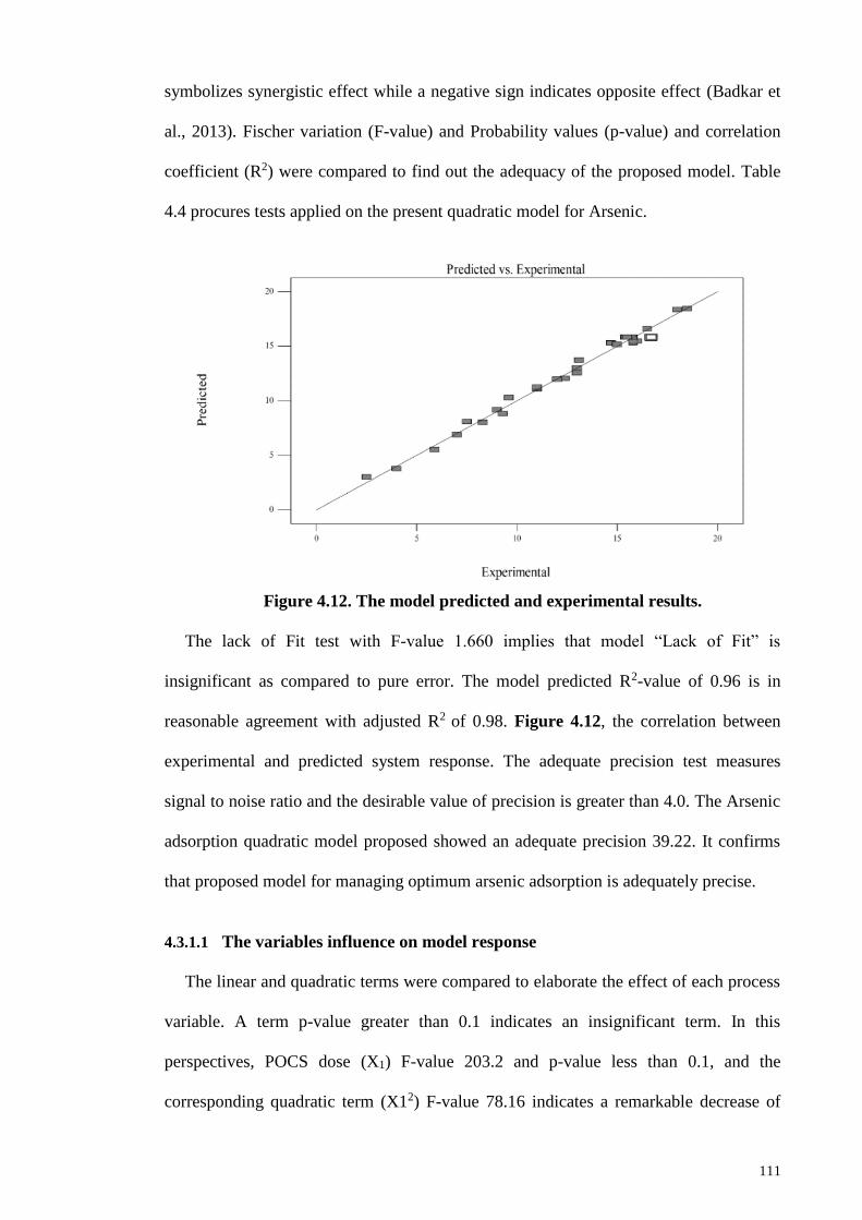
111
symbolizes synergistic effect while a negative sign indicates opposite effect (Badkar et
al., 2013). Fischer variation (F-value) and Probability values (p-value) and correlation
coefficient (R2) were compared to find out the adequacy of the proposed model. Table
4.4 procures tests applied on the present quadratic model for Arsenic.
Figure 4.12. The model predicted and experimental results.
The lack of Fit test with F-value 1.660 implies that model “Lack of Fit” is
insignificant as compared to pure error. The model predicted R2-value of 0.96 is in
reasonable agreement with adjusted R2 of 0.98. Figure 4.12, the correlation between
experimental and predicted system response. The adequate precision test measures
signal to noise ratio and the desirable value of precision is greater than 4.0. The Arsenic
adsorption quadratic model proposed showed an adequate precision 39.22. It confirms
that proposed model for managing optimum arsenic adsorption is adequately precise.
4.3.1.1 The variables influence on model response
The linear and quadratic terms were compared to elaborate the effect of each process
variable. A term p-value greater than 0.1 indicates an insignificant term. In this
perspectives, POCS dose (X1) F-value 203.2 and p-value less than 0.1, and the
corresponding quadratic term (X12) F-value 78.16 indicates a remarkable decrease of

112
the F-value. It can be interpreted as an increase in POCS has resulted in a decrease in its
effect on Qe, during fixed pH, temperature and arsenic initial concentration (mg L-1).
Similarly, linear term of As initial concentration (X2) has F-value 254.0 and p less than
0.0001. X22 has F-value 93.4 and p less than 0.0001. It means that both linear and
quadratic terms for initial concentration are significant.
Table 4.4. Arsenic adsorption statistical analysis results.
Source of variation df SS MS F P-value
Regression 14 514.63 36.76 118.44 < 0.0001
Residual error 15 4.66 0.31 - -
Lack of Fit (model error) 10 3.58 0.36 1.66 0.299
Pure Error (replicate
error) 5 1.08 0.22 - -
Total 29 519.28 - - -
R2 0.991
Abbreviations: df= degree of freedom; SS=sum of squares; MS= mean squares.
Moreover, the relative values show that initial concentration beyond optimum has
resulted in a declined arsenic adsorption. Temperature linear term (X has F-value 50.01
and p less than 0.0001 while quadratic term (X32) has F-value 28.25 & p less than
0.0001. These comparative values of respective statistical terms indicate a relatively
lesser effects of temperature as compared to other variables in present design of
experiment. The most prominent variable was pH (X42) in this study. The variable pH
showed a relatively higher impact on adsorption as can be seen in its relatively high F-
value 745.6. The quadratic term of pH was still dominant on other variables. A
comparison among linear and quadratic terms describes the relative influence of linear
and quadratic terms for the variables competitive role during adsorption. It is beauty of

113
RSM design of study as it explain combined effects of interactive variable, as compared
to OVAT strategy of experiments (Witek-Krowiak et al., 2014).
4.3.1.2 RSM 3D plots
Figure 4.13 portrays the response surfaces (RSM 1 to 6) the three dimensional
model presentation to discover the optimum adsorption. It is interesting that the
response surface method not only explains shared effects but also support optimum
variable ranges for optimum adsorption. Figure 4.13 (RSM 1) shows a combined effect
of arsenic initial concentration (mgL-1) and POCS dosage (mg). It is observed that
arsenic initial concentration has more influence on Qe as compared to adsorbent dose.
For instance, POCS dose in the range from 500 to 1000 mg at a fixed pH 4.0 and
temp.25oC increases Arsenic Qe from 4.0 to 5.9 mg g-1. Conversely, an increase in
initial concentration of from 100 to 250 mg L-1 (pH 4.0 and temperature 25oC) bring
about a double increase of Qe from 4.0 to 9.0 mg g-1. The RSM 1 projected maximum
Qe ~18.0 mg g-1 with 1.0 g adsorbent dosage and 250 mg L-1 arsenic. Figure 4.13 (RSM
2) depicts effects of temperature and POCS dose on Arsenic. The RSM 2 shows direct
influence from temperature on Qe, indicating an endothermic reaction during the arsenic
adsorption. Relatively, it shows lesser effect. E.g. during fixed adsorbent dose, pH and
initial concentration, temperature increase from 15 to 55oC resulted in a slow increase in
Qe from 12.0 to 15.0 mg g-1. RSM 3 Qe increases regularly with pH and dose. The
variable range of pH exhibited leading role as compared to dose of adsorbent in this
study. E.g. at a fixed dose 1.0 g, temperature 45oC and initial concentration the pH
increase resulted in a dramatic increase in Qe from 13.0 to 18.5 mgg-1. Figure 4.13
(RSM 4) displays the effect of temperature and initial concentration. It shows that an
increase in arsenic concentration goes linearly with Qe when other variables were held
constant. Figure 4.13 (RSM 3) uncovers the combined i.e. pH and POCS dose effect.

114
Figure 4.13. 3D response surface plots. RSM 1 Arsenic initial Conc. (mg L-1) and
POCS dose (mg) RSM 2 Temp vs POCS dose (mg). RSM 3 Initial pH vs POCS
dose (mg) RSM 4 Temp. vs Arsenic initial Conc. (mg L-1). RSM 5 pH vs Arsenic
initial Conc. (mg L-1) RSM 6 pH and Temp (oC).
From The relative increase in Qe can be credited to the higher number of effective
collisions and high concentration. Likewise, temperature provides the kinetic energy for
more effective collisions and improved adsorption. The two process variables work for
a better Qe. However after optimum a further increase in both variables decreases Qe as
understood in RSM 4. The reason for decrease in Qe is attributed to the increased

115
velocity of molecules and a widening of pores at elevated temperatures. Figure 4.13
(RSM 5) illustrates an effect of pH and arsenic initial concentration on Qe. In an
experiment with POCS 750 mg, arsenic initial concentration 175 mg L-1 and
temperature 35oC an increase in pH from 6.5 to 11.5 changes Qe from 16.7 to 15.81 mg
g-1. The results indicated that at elevated concentration, increase in pH has
comparatively slighter effect on adsorption process. Figure 4.13 (RSM 6) shows the
effect of pH and temperature at a static POCS dose and arsenic concentration. The
response surface also explains optimum Qe within a dynamic range of pH and
temperature. The response surfaces optimizations experiments results explain the
connections among selected variables and the synergistic effects on adsorption. The
model presented a suitable design to realize optimum adsorption efficiency by
controlling the ranges of the respective input variables.
4.3.1.3 2D adsorption contour plots (CPs)
Figure 4.14 shows the 2D CPs (1 to 6) regarding optimum area of adsorption for
batch mode adsorption design based on CCD strategy. The CPs explain the common
influence of two variables on adsorption (Bilici Baskan et al., 2010; Roy et al., 2014). In
this study, the CP1 displays the effect of POCS dose (mg) and As (mg L-1). A regular
increase in Qe with a corresponding change in dose and concentration variables can be
seen from this design. Nevertheless, outside optimum contour lines yet again display
area with a Qe drop from the optimum (Figure 4.14 CP1). The CP1 likewise shows a
middle red zone area of the contours circles for a maximum of Qe 17.3 mg g-1. The CP2
proves the effect of dose (mg) and temperature whereas the other variable are kept
constant. The middle red zone shows a maximum Qe followed by yellow, green and
blue areas in a decreasing order. The CP3 portrays the effect of dose (mg) and pH at a
constant As initial concentration (mg L-1) and temperature.
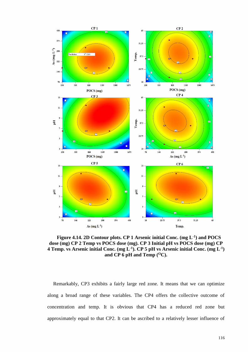
116
Figure 4.14. 2D Contour plots. CP 1 Arsenic initial Conc. (mg L-1) and POCS
dose (mg) CP 2 Temp vs POCS dose (mg). CP 3 Initial pH vs POCS dose (mg) CP
4 Temp. vs Arsenic initial Conc. (mg L-1). CP 5 pH vs Arsenic initial Conc. (mg L-1)
and CP 6 pH and Temp (OC).
Remarkably, CP3 exhibits a fairly large red zone. It means that we can optimize
along a broad range of these variables. The CP4 offers the collective outcome of
concentration and temp. It is obvious that CP4 has a reduced red zone but
approximately equal to that CP2. It can be ascribed to a relatively lesser influence of
117
temperature in this study. The CP5 reveals a synergistic consequence of pH and As
concentration. The responsible adsorption variables has proved to be the most
influencing as the effect on broad red zone is clear from CP5. Finally, the CP6 presents
the reasonable effects of pH and temp. Once more time the pH stands out as a dominant
adsorption variable as it broadened area of middle contour considerably. Arsenic
adsorption results visibly detailed the effects of four variables to accomplish optimum
adsorption.
From the results of DOE strategy for Arsenic adsorption we deduced following
conclusions: The indigenous POCS bears suitable adsorbent properties for Arsenic e.g.
water absorption, specific gravity and fitness modulus. The selected dimensions of the
adsorbent possess rich surface functional groups along with the micro porous
networking that supports outstanding adsorption. All the selected variables influence the
adsorption and were found statistically significant process variables. The strong
correlations between predicted and experimental results proves the accuracy and
precision of the model. RSM and CPs visualize the effect of variables on the Arsenic
adsorption in 3D and 2D fashion respectively. The model finding suggest that a
systematic environmental management strategy with indigenous renewable adsorbents
resources can be designed to reuse and recycle abundant volumes of agro industrial
waste.
4.4 Modelling Acephate adsorption.
The green natural abundant resource from palm oil industry is a versatile material
with diversified functional groups, pore structure, mechanical strength and ability to
form various grades of natural adsorbents. Impressed by its natural properties, various
experimental parameters and their effect on adsorption of acephate have been studied
for their impact to remove an organophosphorous group’s pesticides from hydrological

118
samples. The present study only focused on the three main types of models i.e. i.
Isotherms models ii. Kinetic models and iii. Thermodynamics models. The equilibrium
adsorption data is subjected to various adsorption isotherms (Langmuir, Freundlich,
Flory-Huggins (FH), Dubinin-Radjuvic (DR) and Temkin).Pseudo-first order, second
order and intraparticle diffusion kinetic models are used for kinetic studies.
The frequent application of pesticides is being exercised in most of the agricultural
countries to control the crops damages by pests. However the proper care to protect the
natural environments from unwise or accidental discharge of these toxic molecules into
aquifer raises our concern to protect natural environment. There are many classes of
pesticides but we selected organophosphorous group (OPPs) of pesticides and more
specifically Acephate (AP) (Figure 4.15). The AP is known to cause toxic effects in
vertebrates, for example, affecting central nervous system (CNS) (Aragay et al., 2012),
respiratory (Tian et al., 2012) and reproductive systems (Salameh et al., 2003) and also
adverse genetic changes in the genetic code (DNA) (Singh et al., 2011).The AP is an
insecticide for controlling the sucking and biting insects. However its discharge into
waters, air and soil is a serious cause of environment quality degradation over time. At
present various technologies for pollutants removal e.g. liming, photo-degradation,
catalytic degradation have been implemented including adsorption as the superior
choice due to the availability of adsorbents and reuse and recycle capabilities.
Adsorption is a versatile technique having many practical advantages over the other
water treatment techniques. It exploits interplay of complex phenomenon that is sorbate-
sorbent interactions, surface phenomenon, matrix matching effects, electrostatic effects,
types of bonding.

119
Figure 4.15 Molecular structure of Acephate (AP).
The role of ultrasound assisted rapid mixing of sorbate and sorbent molecules leads
to many faster steps involved in chemical kinetics (Entezari et al., 2005). The use of
ultrasound increases the mass transfer rate by reducing diffusion resistance (Schueller et
al., 2001; Zheng et al., 2005). The present study explores the use of ultrasound assisted
rapid mixing to facilitate the different steps of adsorption that is bulk diffusion, film
diffusion, pore diffusion and chemical binding with the sorbent (POC) (Renault et al.,
2008). Acephate was only chosen to develop isotherms i.e. Langmuir, Freundlich,
Dubinin-Radushkevich and Florry Huggin model. The Isotherms were developed at two
distinct temperatures i.e. 293 K and 313 K respectively. The detailed parameter are
given in Table 4.5 “Isotherm results for Acephate. Moreover the model results are
completely discussed in sub-section 4.5.3, along with all the experimental parameters in
details. It was also exercised to study the Kinetics model i.e. Pseudo-first order, Pseudo-
second order and intra-particle diffusion model recommended model for such type of
studies. The recommended model were only selected after careful consideration of the
current literature to support such type of studies. Moreover the full details of the each
model parameters are clearly mentioned in Table 4.6 and fully discussed in sub-section
4.5.4.
4.4.1 HPLC for acephate
The POC was taken in a glass vial along with the addition of small quantity of HPLC
mobile phase in a ratio H2O-ACN (20:80). The known amount of AP was placed in the
ultrasonic bath for the pre-determined optimized time interval. After that it was taken
out, filtered out the solid sorbent particles and immediately injected into HPLC (D-Star

120
Instruments 8424 Quary Rd., VA 20110–800-DSTAR12), equipped with a Mightysil
RP-18, GP 250-4.6 (5µm) column and UV–Vis detector, at 215 nm wavelength (Figure
4.16).The percent of Acephate (% AP) can be obtained using the following Equation
4.4:
% AP = Area of sample peak
Area of Std. peak X
Wt. of Standard
Wt. of SampleX % Purity of Std.
Equation 4.4
Figure 4.16 HPLC schematic
4.4.2 Sonication time optimization
An Ultrasonic bath with temperature control conditions was used to study sonication
effects. The sonication time was optimized with 1.0 mL Acephate (100 mgL-1), taken in
a vial with fixed amount of POC adsorbent. The sorption was determined after different
time intervals. The time based studies of AP revealed initially the AP uptake was
relatively faster, it became slower towards the equilibrium point. It is explained, at the
start of sorption, there were more vacant surface sites on POC available for AP
adsorption.

121
4.4.3 Isotherm models for acephate
The chemical equilibrium was studied using 0.01g of POC, varying the initial AP
from 25 mgL-1 to 300 mgL-1, pH 3.0 and temperature at 293K and 313K.. Chemical
equilibrium studies were performed at 293 K and 313K at pH 3.0, dose 0.01g, initial
concentration of acephate 25-300mgL-1 with 3.0 min sonication time and the results are
given in the Table 4.5. Langmuir parameters Qmax, KL, RL and aL are given in Table 4.5.
The factor aL decreases with increase in temperature representing a decrease in sorption
capacity with temperature as shown in Figure 4.17. The RL parameter describes whether
the adsorption process is favorable: The RL parameter is less than 1 but greater than 0,
indicating the feasible sorption process. The Freundlich parameter n and KF are in good
agreement with the Langmuir parameter RL, KL and 𝑎𝐿. It is clear from Table 4.5, that
the value of Temkin constants KT and Bt decreases with an increase in temperature,
indicating an exothermic sorption process. The DR isotherms adsorption energy
indicated the exothermic adsorption as the value of E decreases from 201.779 KJ mol-1
to 148.278 KJ mol-1 with an increase in temperature from 293K to 313K.

122
Table 4.5 Isotherms results for Acephate.
Isotherm model Temperature
293K 313 K
Langmuir
Qmax (mg/g) 11.228 10.667
KL (L/g) 0.651 0.323
aL(L/mg) 0.0295 0.0251
RL 0.0548 0.0854
R2 0.994 0.991
Freundlich
n 3.2 1.9
KF (mg/g) 2.57 2.29
R2 0.895 0.901
Temkin
KT (L/g) 0.332 0.198
Bt (mg/g) 5.24 4.04
R2 0.9472 0.9321
Dubinin-Radushkevich
Xm (mg/g) 9.517 8.341
Β 3.1E-05 1.9E-05
E (KJ/mol) 301.8 160.3
R2 0.9605 0.9521
FH Model
n 2.1418 3.3459
KFH 0.0357 0.0286
R2 0.8761 0.8978
The FH model parameter for the extent of adsorbate surface coverage also supported
the previous results as the value of “n” model parameter increase from 2.142 to 3.36
with a corresponding increase of temperature.

123
Figure 4.17 I-1, I-2, I-3, I-4 and I-5 represent Freundlich, Langmuir, Temkin,
DR and FH Isotherms respectively.
Figure 4.18 a comparison of Qe predicted by different isotherm models.

124
4.4.4 Kinetics models for Acephate
The Kinetic experiments were performed at 293K and 313K using the 100 mgL-1 of
acephate, 0.01g of adsorbent dose, pH 3.0 with different sonication time intervals. The
adsorption capacity at any time interval “t” was determined by: Equation 4.5,
adsorption capacity with time “Qt”.
𝑄𝑡 =(𝐶𝑜 − 𝐶𝑡)𝑉
𝑚
: Equation 4.5
Table 4.6 Acephate Kinetic models results.
Kinetic model Temperature
293K 313 K
Pseudo-first-order
Qe (exp.)/mg g-1 11.607 11.081
K1 (min-1) 0.014 0.015
R2 0.978 0.969
Pseudo-second-order
Qe (model)/mg g-1 12.427 12.280
k2 (g mg-1min-1) 0.0014 0.001
h /mg g-1min-1 0.3058 0.287
t1/2/ min 169.183 165.730
R2 0.998 0.996
Intraparticle diffusion
I (model)/mg g-1 5.040 4.642
Kid (g mg-1min-1) 0.508 0.509
R2 0.925 0.966

125
The value of constants K2 (g.mg-1min-1) and Qe (mgg-1) are given in the Table 4.6.
According to correlation coefficient values, the 2nd order model is more suitable to the
Acephate adsorption kinetic data than that of the first order model. Table 4.6 shows that
the value of Qe decreases by increasing the temperature. It is an established fact that the
value of intraparticle parameter “I” is directly proportional to the boundary layer
thickness (Bekçi et al., 2008). The Value of I (Table 4.6) shows a deviation of model
curve from origin which means that surface adsorption and intraparticle diffusion steps
are operating simultaneously during the adsorption process Figure 4.19.
Figure 4.19, K1, K2, K3 show the 1st , pseudo 2nd and intraparticle diffusion
models respectively.
Figure 4.20. Comparison among experimental and model predicted results for
AP adsorption.
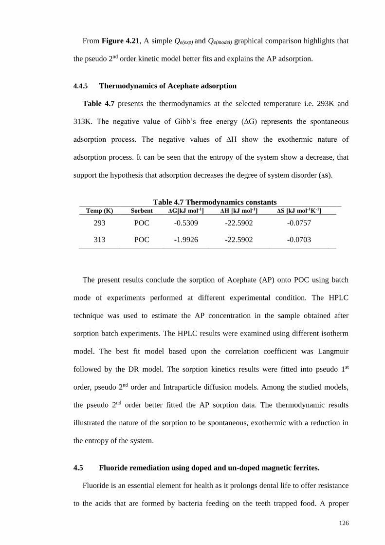
126
From Figure 4.21, A simple Qe(exp) and Qe(model) graphical comparison highlights that
the pseudo 2nd order kinetic model better fits and explains the AP adsorption.
4.4.5 Thermodynamics of Acephate adsorption
Table 4.7 presents the thermodynamics at the selected temperature i.e. 293K and
313K. The negative value of Gibb’s free energy (∆G) represents the spontaneous
adsorption process. The negative values of ∆H show the exothermic nature of
adsorption process. It can be seen that the entropy of the system show a decrease, that
support the hypothesis that adsorption decreases the degree of system disorder (ΔS).
Table 4.7 Thermodynamics constants Temp (K) Sorbent ΔG[kJ mol-1] ΔH [kJ mol-1] ΔS [kJ mol-1K-1]
293 POC -0.5309 -22.5902 -0.0757
313 POC -1.9926 -22.5902 -0.0703
The present results conclude the sorption of Acephate (AP) onto POC using batch
mode of experiments performed at different experimental condition. The HPLC
technique was used to estimate the AP concentration in the sample obtained after
sorption batch experiments. The HPLC results were examined using different isotherm
model. The best fit model based upon the correlation coefficient was Langmuir
followed by the DR model. The sorption kinetics results were fitted into pseudo 1st
order, pseudo 2nd order and Intraparticle diffusion models. Among the studied models,
the pseudo 2nd order better fitted the AP sorption data. The thermodynamic results
illustrated the nature of the sorption to be spontaneous, exothermic with a reduction in
the entropy of the system.
4.5 Fluoride remediation using doped and un-doped magnetic ferrites.
Fluoride is an essential element for health as it prolongs dental life to offer resistance
to the acids that are formed by bacteria feeding on the teeth trapped food. A proper

127
washing of teeth and regular tooth brush activities is a simple solution to overcome
dental decay or plaque formation. Fluoride consumption is reportedly increasing beyond
maximum permissible limits that is believed to cause health problems (Bain et al., 2012;
Gonzalo et al., 2012; Shen et al., 2003). The maximum allowable concentration level
(MCL) of 1.5 mg/L fluorides has been recommended by World Health Organization
(WHO). The drinking of lots of fluorides results into impaired growth, intelligence,
arthritis, skeletal deformations, osteoporosis and even cancer in severe cases (Kang et
al., 2011; Ma et al., 2014; Onyango et al., 2004; Velazquez-Jimenez et al., 2013; Yadav
et al., 2007). The present problem of fluorides access in consumer water give an idea to
make an adsorptive removal strategy using some series of magnetic ferrites.
“[However, some problems remain in the development of adsorbents for fluoride
adsorption, such as instability, matrix effects, mechanical strength and poor adsorption
capacity. Therefore, more efforts should be devoted towards new classes of adsorbents
with high de-fluoridation capacity. In recent times, magnetic adsorbents with competent
adsorption capacities and environmental friendly properties have been designed,
developed and applied for the treatment of anionic waste products, such as fluoride,
nitrate, sulfate, arsenate and phosphate. The magnetic adsorbents include magnetic
materials, such as iron, copper, cobalt and nickel oxides (Hua et al., 2012). The flexible
geometric structures of transition metal oxides allows the manufacture of adsorbents
with exceptional properties (Rao et al., 2012). The cubic close packed geometry of
CuFe2O4 offer two types of sites, i.e., tetrahedral sites (A) and octahedral sites (B)
(Gadkari et al., 2009). The electrical and magnetic properties depend on the position of
each metal on each site. These sites play a deciding role in the electromagnetic
properties (Ahmed et al., 2006). Ferrites exhibit the trade of electrons during Fe-Fe
interaction, causing polarizations and electrical conductivity (Ahmed et al., 2006).
However, doping rare earth cations alters the electrical, magnetic and physical

128
properties (Kobayashi et al., 2002; Zhao et al., 2008). For instance, Cerium (Ce) is a
unique single electron system; it enables particle dispersion, which is a anticipated and
expected properties for an adsorbent. Cerium also promotes a larger number of active
functional sites, surface area, and a larger pore size and pore volume. These
improvements expedite the adsorbate-adsorbent interactions because the adsorbate can
straightforwardly diffuse and reach the active sites for adsorption.]
[The ion chromatographic (IC) parting and detection method for quantifying anions
provides numerous benefits. First, only a small amount of sample (20 µL) is required,
which permits for the separation of associated ions, depending on the retention times
(tR). Second, aligned ion suppressor controls the conductivity by suppressing the
concomitant ions, in this manner causing high conductivity. Third, a number of anions
can be concurrently spotted and quantified in a single run due to the specific interaction
and partition amid the stationary phase and the mobile phase. Besides, IC separation is a
highly specific, selective, reproducible, robust and cost-effective method.]
[Electric, magnetic and dielectric behavior of ferrites is a function of structural
properties (Ahmed et al., 2015; Larbi et al., 2015; Larbi et al., 2014). Therefore XRD,
ATR and FESEM are especially used for adsorbent characterization. High penetrating
power, X-rays provides important information regarding structural properties of the
matter. Every material is distinctive due to its size of atoms, arrangement of atoms and
ability to scatter X-rays. Since no two atoms have exactly same size and X-ray scatter
ability, the intensities of diffracted beam will be only one of its kinds for every material.
This individuality helps to identify the structure and determine the structural parameters
of the material (Gadkari et al., 2009). Multiphase structure, crystallite sizes and crystal
strains of CuCexFe2-xO4 were observed by XRD, (PANanalytical`s Emprean), equipped
with a monochromatic Cu Kα radiation source. Ferrites surface morphology, particle

129
size distribution were studied by FESEM. FTIR analysis was performed on a Perkin
Elmer System 2000 series spectrophotometer (USA) between 4000-400 cm-1. Magnetic
hysteresis loops were recorded on VSM. BET specific surface area study of the samples
was carried out on the basis of nitrogen adsorption desorption isotherms measured at
77K using a BELSORP-max nitrogen adsorption equipment (Japan Inc.). CV and EIS
experiments were carried out on Autolab PGSTAT 302N and NOVA 1.10 software for
the analysis of data.
4.6 Characterization of doped and undoped magnetic ferrites
4.6.1 XRD analysis
[In the absence of cerium (x=0.0), all of the identified peaks match with copper
ferrite (CuFe2O4), indicating the creation of spinel-type CuFe2O4 (Mexmain, 1971).
After the addition of Ce (x=0.1), some additional peaks of low intensity appeared in the
XRD spectra corresponding to CeO2 (Wyckoff, 1963). The accumulation of cerium into
the pristine copper ferrite showed distinct variation in the percentages of the respective
phases. The organized increase in dopant concentration (x) caused in a gradual increase
in the intensity of the CeO2 peaks. Moreover, we observed a decline in the (311) peak.
A judgment among the crystallite sizes divulges a regular fall of crystallite size with a
gradual increase in dopant (Ce). Table 4.8 shows that while doping copper ferrites with
Ce reduced the crystallite sizes of pristine ferrite.]

130
[Table 4.8. Crystal sizes and the micro-strain and BET properties of a series of
copper ferrites CuCexFe2-xO4 (x=0 to 0.5).
Property x=0.0 x=0.1 x=0.2 x=0.3 x=0.4 x=0.5
BET Surface area
(m2/g) 70 75 79 83 88 92
Crystallite sizes D
(nm) 72 50 34 30 20 18
Average pore size
(nm) 38 34 30 25 20 17
Pore volume (cm3/g) 0.44 0.4 0.38 0.34 0.29 0.26
Lattice strain η (%) 0.17 0.25 0.38 0.42 0.64 0.69
This decrease was attributed to the formation of secondary phases (Khandekar et al.,
2013). This decrease was also supported by a relative increase in the lattice parameters.
Accordingly, the Ce3+ ions were oxidized to Ce4+ at this temperature and appeared as a
separate phase in the XRD spectrum (Figure 4.21).]
[The surface properties, surface area, and pore size and volume of the adsorbents
were analyzed via BET. [Table 4.8] indicates that a measured increase in dopant
concentration (x) parallels to an increase in the BET surface area. Cerium oxide likely
constrains the growth of larger particles because of its high dispersion (Zhao et al.,
2008). The BET results indicate that during adsorption, more fluoride can interact with
the available active sites that are created by doping in these magnetic ferrites.]

131
Figure 4.21. XRD spectra [A] un-doped CuFe2O4, [B] doped CuCe0.1Fe1.9 O4, [C]
CuCe0.2Fe1.8 O4, [D] CuCe0.3Fe1.7 O4, [E] CuCe0.4Fe1.6 O4, and [F] CuCe0.5Fe1.5 O4
adsorbents for fluoride, annealed at 650 °C for 3 h.
4.6.2 Electro-analytical results
The electrochemical properties of ferrite modified electrodes were studied using
electrochemical impedance spectroscopy (EIS) (Figure 4.22). The EIS technique
measures the charge transfer resistance (Rct) and parting efficiency between the holes
and electrons. The studied Rct is a critical factor in the charge separation efficiency. The
arc radius shrinkages from x=0 to x=0.2, which indicates higher charge resistance with
higher Ce content. According to the hopping mechanism, changes in the mobility of the
charge carriers lead to the transmission of current by hopping from one iron atom to the
next (Rezlescu et al., 2000). When cerium is doped in the place of iron, the resistivity of
the sample is found to increases. This behavior can be explained by the greater
resistivity of cerium (74.4 × 10⁻⁸Ω m) compared with iron (8.57 × 10⁻⁸ Ω m) (Lamarca
et al. (2005). Further increase in the Ce dopant in the range of x=0.3 to x=0.5 again
uncovers that larger semicircles are associated with the higher amounts of Rct. The LSV
analysis was used to study the electrochemical properties of the adsorbents.

132
Figure 4.22. (A) Effect of the applied potential on the current response and (B)
Nyquist diagrams of (x=0) un-doped CuFe2O4 (x=0.1), doped CuCe0.1Fe1.9 O4
(x=0.2), CuCe0.2Fe1.8 O4 (x=0.3), CuCe0.3Fe1.7 O4 (x=0.4), and CuCe0.4Fe1.6 O4
(x=0.4) CuCe0.5Fe1.5 O4 in 0.1 M KCl solution containing 1.0 mM K3[Fe(CN)6 ] and
K4 [Fe(CN)6 ] (1:1).
Ferrite with x=0.2 exhibited the maximum photocurrent response, followed by x=0.1.
The photo-electrochemical activity is well known to be determined by the light
harvesting capacity and the separation of electron-hole pairs (Zhang et al., 2014).
Generally, a high value of the photocurrent indicates that the sample has a strong ability
to generate and transfer the photo-excited charger carrier under irradiation. The EIS and
LSV results confirm that the ferrite adsorbents can be used as photo-catalysts and
photo-electrode materials in addition to their excellent adsorbent properties.
4.6.3 FTIR of spinel ferrites
“The inter-metallic ionic mode of vibration in FTIR spectroscopy analysis provides
information regarding the ions involved in the formation of the crystal lattice (Borhan et
al., 2013; Zhang et al., 2014). The characteristic peaks of the spinel structure observed
in the range of 560 to 580 cm-1 are attributed to Fe-O stretching vibration at the
tetrahedral site (Figure 4.23). FTIR functional groups were compared in pristine and
Ce-doped ferrites. All Ce-doped ferrites have distinct peaks near 850 cm-1 and 1440 cm-

133
1. The additional functionality is thought to be responsible for the electrostatic
interaction with the adsorbate to enhance the overall fluoride adsorption. The hydroxyl
and sulfate groups are clearly involved in the fluoride adsorption. The abundance of
these groups in the Ce-doped ferrite may be the main reason for the high fluoride
uptake.”
4.6.4 FESEM results
“When x=0.0, we observe normally sized CuFe2O4 nano-crystals (~74 nm) with
uniform morphology along with some agglomerations of larger size (~180 nm). This
behavior was due to the large specific surface of the fine particles for van der Waals
interactions. From a Nano chemistry perspective, adjacent nanoparticles that share a
common crystallographic orientation may collide with each other, which leads to
coalescence (Balaz, 2008) because adjacent primary particles attach to each other and
form aggregates.”
Figure 4.23. FTIR overlay spectra of (A) un-doped CuFe2O4, (B) doped
CuCe0.1Fe1.9 O4, (C) CuCe0.2Fe1.8 O4, (D) CuCe0.3Fe1.7 O4, (E) CuCe0.4Fe1.6 O4, and
(F) CuCe0.5Fe1.5 O4.

134
“In addition, due to the nanometer-scale sizes, these particles continue to collide and
coalesce to form even larger particles. This phenomenon may eventually cause
agglomeration in the fabricated ferrites. The agglomeration is affected by various
processing parameters, such as speed, intensity and mixing time. Relatively smaller
sizes were observed with further addition of ceria (x=0.1 to x=0.5). Moreover, the
addition of ceria particles was found to increase the surface area by allowing for
maximum dispersion and retarding large grain growth (Figure 4.24). These results
complement the XRD results and provide evidence of an increased surface area, which
can facilitate better fluoride adsorption. These results also agree with those of other
studies, indicating that doping lanthanides delays particle grain growth (Ishaque et al.,
2015; Khandekar et al., 2013). The observed incremental diminution in grain
morphology via the orderly doping of ceria promotes fluoride adsorption.”

135
Figure 4.24. FESEM images of (A) un-doped CuFe2O4, (B) doped CuCe0.1Fe1.9 O4, (C) CuCe0.2Fe1.8 O4, (D) CuCe0.3Fe1.7 O4, (E) CuCe0.4Fe1.6
O4, and (F) CuCe0.5Fe1.5 O4 prepared in micro-emulsion (w=15).

136
4.6.5 Magnetic properties
“The value of the squareness ratio (SQ) was analyzed by dividing the value of the
magnetic remanence (Mr) by the magnetic saturation (Ms) (Appendix E). The SQ value
reflects the magneto-crystalline anisotropy and the super-exchange interactions of the
ferrite series (Chinnasamy et al., 2003). CuFe2O4 exhibits a SQ value of 0.13 (x=0.0),
but after Ce doping, this value increases in the cases of x=0.1 and x=0.2. Note that the
incorporation of Ce reduced the magneto-static interactions (Domingo et al., 2012).
However, the further supplement of Ce exhibits a regular declining inclination from
x=0.3 to x=0.5. This phenomenon indicates that the local canting effect is taking control
over the surface canting effects associated with crystallite size and coercivity (Wahba et
al., 2015). The relative change in Mr and Ms with Ce content has exactly the same
trend, as expected from the SQ values for each member of the series Table 4.9.”
Table 4.9. Magnetic properties of the CuCexFe2-xO4 adsorbents by VSM.
Magnetic parameters
0.0 0.1 0.2 0.3 0.4 0.5
Coercivity (T) 0.007 0.009 0.010 0.01 0.009 0.004
Ms (emu/g) 30.14 25.31 15.53 13.01 11.65 8.89
Mr (emu/g) 4.34 3.89 3.09 2.50 2.11 0.82
SQ
0.14 0.15 0.20 0.19 0.18 0.09
The Hc value is obviously increasing with the quantity of dopant (x from x=0.0 to
x=0.2), and further doping results in a regular decline (from x=0.3; the maximum
decrease occurs when x=0.5), which is credited to extrinsic and intrinsic factors. The
extrinsic factors depend on the density, morphology and grain size (Potts et al., 2011).
The intrinsic factors, such as relative occupation of sub-lattice sites, contributed to the
magnetism in the nano-ferrites (Raju et al., 2014). The shape and width of the hysteresis
loops depend on the method of preparation, composition, and distribution of the metal

137
cations at the tetrahedral and octahedral sites, the spin canting and the crystallite size
(Borhan et al., 2013). The values of Mr and Ms exhibit a regular decline. This behavior
could be described by the decrease of D from 73 nm to 18 nm, and the respective
increase in the Ce content at the B-sites. Because the magnetic moment of Ce is less
than that of Fe, theoretically, increasing the Ce content will reduce the Ms
monotonically (Petrovic et al., 2001; Wahba et al., 2015). Generally, rare-earth elements
have a strong anisotropic subsystem with a adequately high anisotropic exchange
constant for iron (Gornostaeva et al., 2013). Thermal excitation breaks the Kondo state,
which causes a gradual recovery of magnetic moments (Buschow, 2005).”
“Ce3+ magnetic moments are managed by direct or indirect exchange interaction,
namely RKKY interaction facilitated by conduction electrons (Fikáček et al., 2013).
Appropriately strong exchange interaction produces a magnetically ordered ground
state. However, in the case of x=0.3, a dominance of the Kondo interaction occurs,
which results in a nonmagnetic ground state. A variation in the coercive field (Hc)
directly depends on the surface spin disorder (Kostopoulou et al., 2014). The decrease in
Hc of the present series affirmed the reduced surface spin disorder. The magnetic
properties of the ferrites are controlled by Fe-Fe interaction via the spin coupling of 3d
valance electrons (Dixit et al., 2012). The present decrease in coercivity is assigned to
morphology-increased magnetic moments and domain wall migration (Niaz Akhtar et
al., 2014). The lower values of Mr and Ms are due to the oxidation of cerium into
diamagnetic states (Dutta et al., 2006). However, the present decrease in magnetic
character has little effect on the fluoride adsorption capacity, but it affects the magnetic
separation capability due to the change in its morphology, crystal structure and related
electromagnetic properties.”

138
4.6.6 Ion chromatography separation results
“The anions were identified and quantified based on their retention time (tR) when
performing Ion chromatography (IC), as presented in Table 4.10. Anion calibration
standards of 1, 5 and 10 mgL-1 were run to develop a calibration method. The tR values
of standards and samples were compared and quantified with MagICNetTM1.0. In
suppressed ion chromatographic separation, an ion suppressor was inserted between the
separating column and the detector to reduce the inherent conductivity of the eluent for
improved anion detection. The reactions involved with the chemical suppressor are
represented by the following equation (Eith et al., 2001).”
Figure 4.25. Magnetic properties of (A) un-doped CuFe2O4, (B) doped
CuCe0.1Fe1.9 O4, (C) CuCe0.2Fe1.8 O4, (D) CuCe0.3Fe1.7 O4, (E) CuCe0.4Fe1.6 O4, and
(F) CuCe0.5Fe1.5 O4.
Table 4.10. Retention times of the selected anions during ion chromatography.
Anions F- Cl- NO3- SO4
2-
tR 4.05 5.54 8.87 16.60

139
“Na+ ions coming in mobile phase are substituted with H+ ions, reducing the
conductivity of the background electrolyte, as represented by Equation 4.46. The anion
in sample, e.g., F- remains unchanged by the suppressor, detected and quantified by IC
system, as represented by Equation 4.57.”
Equation 4.4. Reaction in chemical suppressor
𝑹 − 𝑺𝑶𝟑−𝑯+ + 𝑵𝒂+ + 𝑯𝑪𝑶𝟑
− 𝑹 − 𝑺𝑶𝟑−𝑵𝒂+ + 𝑯𝟐𝑶 + 𝑪𝑶𝟐 Equation 4.6
Equation 4.5. Fluorides for I.C detection.
𝑹 − 𝑺𝑶𝟑−𝑯+ + 𝑵𝒂+ + 𝑭− 𝑹 − 𝑺𝑶𝟑
−𝑵𝒂+ + 𝑯+ + 𝑭− Equation 4.7
4.6.7 Effect of competing anions
“Concomitant anions, such as chlorides, bicarbonate, nitrate, sulfate and arsenate,
commonly exist in surface and ground water. Because these anions compete with
fluorides for adsorbent active sites, their influence on fluoride adsorption was
experimentally studied under different concentrations (0.1, 1.0 and 10 mM). In addition,
arsenate (As), which is a concomitant anion of widespread concern, was studied at four
different concentrations (2, 5, 10 and 30 mgL-1). The results show that to fluoride
adsorption was affected by the presence of competitive anions. The red, orange, yellow,
green and blue areas highlight the degree of adverse effect, with red indicating the
greatest effect and blue indicating the least effect on fluoride adsorption (Figure 4.26).
In summary, by using a straightforward doping of cerium into magnetic ferrite, we
fruitfully fabricated a series of novel magnetic adsorbents for fluoride adsorption and
water remediation technology. Compared with un-doped parent material, superior
results were obtained, and the present enhancement in adsorption behavior contributed
to the active functional groups created after doping, the increased surface area with
appropriate porosity and the electro-magnetic properties.

140
Figure 4.26. Effect of some concomitant anions on fluoride adsorption, m=0.1 gL-1, [F]0 = 10 mgL-1, pH=7.0: (A) un-doped CuFe2O4, (B)
doped CuCe0.2Fe1.8 O4, (C) CuCe0.3Fe1.7 O4, and (D) CuCe0.5Fe1.5 O4 .
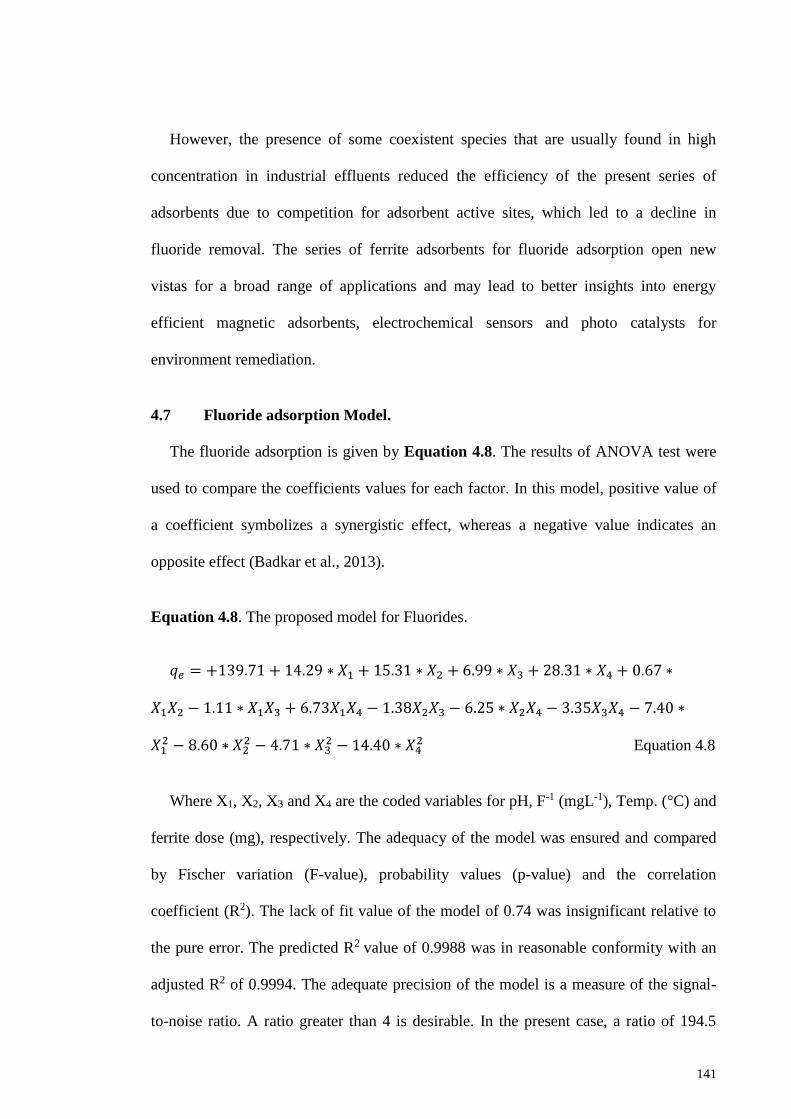
141
However, the presence of some coexistent species that are usually found in high
concentration in industrial effluents reduced the efficiency of the present series of
adsorbents due to competition for adsorbent active sites, which led to a decline in
fluoride removal. The series of ferrite adsorbents for fluoride adsorption open new
vistas for a broad range of applications and may lead to better insights into energy
efficient magnetic adsorbents, electrochemical sensors and photo catalysts for
environment remediation.
4.7 Fluoride adsorption Model.
The fluoride adsorption is given by Equation 4.8. The results of ANOVA test were
used to compare the coefficients values for each factor. In this model, positive value of
a coefficient symbolizes a synergistic effect, whereas a negative value indicates an
opposite effect (Badkar et al., 2013).
Equation 4.8. The proposed model for Fluorides.
𝑞𝑒 = +139.71 + 14.29 ∗ 𝑋1 + 15.31 ∗ 𝑋2 + 6.99 ∗ 𝑋3 + 28.31 ∗ 𝑋4 + 0.67 ∗
𝑋1𝑋2 − 1.11 ∗ 𝑋1𝑋3 + 6.73𝑋1𝑋4 − 1.38𝑋2𝑋3 − 6.25 ∗ 𝑋2𝑋4 − 3.35𝑋3𝑋4 − 7.40 ∗
𝑋12 − 8.60 ∗ 𝑋2
2 − 4.71 ∗ 𝑋32 − 14.40 ∗ 𝑋4
2 Equation 4.8
Where X1, X2, X3 and X4 are the coded variables for pH, F-1 (mgL-1), Temp. (°C) and
ferrite dose (mg), respectively. The adequacy of the model was ensured and compared
by Fischer variation (F-value), probability values (p-value) and the correlation
coefficient (R2). The lack of fit value of the model of 0.74 was insignificant relative to
the pure error. The predicted R2 value of 0.9988 was in reasonable conformity with an
adjusted R2 of 0.9994. The adequate precision of the model is a measure of the signal-
to-noise ratio. A ratio greater than 4 is desirable. In the present case, a ratio of 194.5

142
indicates an adequate signal. The effect of variables was analyzed by comparing the
values of the linear, quadratic and interaction terms. The pH linear term (X1) with an F-
value of 2112.63 indicates the significant role of pH in fluoride adsorption. However,
the pH quadratic term (X12) has an F-value of 2239.4, which is greater than that of the
linear term and indicates a positive role of pH increase in the selected range on fluoride
adsorption. An optimum fluoride adsorption was achieved at neutral pH, as shown in
(Figure 4.27) (RSM A, B and C).
According to the speciation of fluoride, it exists as a HF species instead of ionic (F-1),
which may be the reason for the reduced adsorption under acidic conditions (Yu et al.,
2015). According to the electrostatic interaction mechanism, a comparatively stronger
attraction is observed at a pH below 6.12. However, pH is not the only factor that
controls the fluoride adsorption. In the same way, the linear and quadratic terms of the
fluoride initial concentration are significant during fluoride adsorption. An increase in
the fluoride initial concentration improved the rate of adsorption. However, increasing
the fluoride concentration beyond the optimum reduces the fluoride adsorption, as
shown in (Figure 4.27) (RSM A and D). The linear and quadratic terms of temperature
(X3 and X32) indicate a decrease in fluoride adsorption at elevated temperatures. The
most prominent variable was adsorbent dose (X4), which has a significant influence on
fluoride adsorption. This influence can be explained by the adsorbent dose being
directly related with the number of active sites for fluoride adsorption.”

143
Figure 4.27. Response surfaces showing the effects of two variables on fluoride
adsorption (A) pH and F-1 (mg L-1), (B) pH and Ads. Dose (mg), (C) F-1 (mg L-1)
and Ads. Dose (mg), and (D) Temp. (oC) and Ads. Dose (mg).

144
CHAPTER 5: CONCLUSIONS
5.1 Conclusions
In response to the worldwide environmental contamination contributed by both
natural and anthropogenic sources, two different sources of Nano-adsorbents,
indigenous Palm oil waste and synthetic magnetic ferrites, have been prepared,
characterized and applied for green environment remediation. Studies on adsorbents are
of prime importance to understand the characteristics of the adsorbate-adsorbents
interactions and their efficiency in the removal of hydrological contaminants for the
potential remediation of the hydrosphere. The natural abundantly available palm oil
clinker waste was researched for its versatile surface morphology, green origin and
magnetic separation and application as a renewable resource of natural adsorbent. The
mechanical, physical and chemical treatment were applied to impart the desired
characteristics to the waste biomass.
The primary objective was to convert waste into wealth resource for the betterment
of the agricultural sector that is facing a pollution challenge from the enormous volumes
of bio-waste. A series of adsorbents were prepared based on particle size distribution,
specific gravity, pore size, pore volume and fitness modulus by standard methods. The
reproducibility of experimental adsorption capacity was ascertained by repeating the
experiments to account for standard deviation. The present procedure is robust and
advantageous over arsine gas generation method, as it required no extra reagents to
produce gaseous phase arsenic (arsine gas). The analysis of the adsorption capacity data
was subjected to mathematical modelling. The selected quadratic model provided better
insight into complex correlated, mutually influencing system variables. Unique series of
natural and magnetic Nano-adsorbents were prepared and tested for the hydro
decontamination of heavy metals, organophosphorous pesticides, organic dyes and
anionic water contaminants. The Nano-adsorbents were investigated for the crystal

145
structure, functional groups, thermal stability, morphology and magnetic properties.
Graphene was found to have distinct effects on the surface morphology, crystallite size,
lattice strain, and thermal stability of magnetic Nano-adsorbents.
The average crystallite size and grain size were found to increase, whereas the lattice
strain decreased, with the use of graphene. The Vibrating Sample Magnetometer (VSM)
results indicated that the saturation magnetization and coercivity followed a declining
trend owing to the separation of magnetic centers in the nanocomposite. The fabricated
composite ferrite materials were evaluated to enhance the hydro decontamination
efficiencies for the maximum removal of arsenic, fluorides species along with acephate
(AP), by using the preferred Design of Experiment (DOE) strategy. The adsorption data
was analyzed by isotherm models e.g. Langmuir, Freundlih, Temkin, Dubinin-
Redishkevich (DR), Florry huggins (FH). The present thesis corroborates the efficiency
of Nano-adsorbents under single and dynamic competent environmental conditions. The
adsorption mechanisms was elaborated by the interpretation of pseudo 1st order kinetic
model, pseudo 2nd order and Bhangam’s model. Present work provides a solution for
pollution abatement through the use of novel classes of natural, synthetic and modified
magnetic ferrite adsorbents. It also presents the use of the latest computer software for
strategic application of magnetic Nano-ferrites to reuse industrial waste and remove
toxic pollutants from water.
5.2 Recommendation
Further research for future environmental applications relies on the few continuous
natural resources of adsorbents. The proposed sources of adsorbents can be utilized for
energy free separations or green environment remediation. In case of catastrophic
accidents such as earthquake, floods and distress, these classes of adsorbents provide a
low cost and energy saving alternate solution to provide efficient water decontamination

146
systems. Palm oil industry waste can be reprocessed and exported to the town planners,
situation managers and community users looking for economical adsorbents to protect
and purify water, air and soil. Novel series of adsorbents designed and used for making
nanocomposites with emerging base materials such as graphene and nanotubes of
carbon have long future impacts on public health and social developments. The use of
the DOE strategy resolves the execution and implementation issues e.g. time, efforts
and cost in research and development. The statistically well planned experiments yield
better insight and interaction among the competing process variables responsible for
controlling the adsorption capacities of the Nano-adsorbents. The use of POCS and
magnetic Nano-adsorbents may be extended for industrial process catalysis, reduce
byproducts and protect moisture or air sensitive materials e.g. medicines (Figure 5.1).
Pollutants in the hydrosphere have a direct negative impact on public health and our
combined socio-economic development. The aftermaths of hydrosphere contaminations
embrace toxic waste production, equipment degradation, increased risk to the health and
safety of humans, plants and animals. Henceforward, pollutants in the hydrosphere
require contaminants removal technologies to circumvent the negative consequences of
polluted environments. Nevertheless, the studies of specific magnetic Nano-adsorbents
are still in need of the collaboration from the related agricultural and environmental
businesses.

147
Figure 5.1 Further work plan for future studies.

148
REFERENCES
Abu Qdais, H., & Moussa, H. (2004). Removal of heavy metals from wastewater by
membrane processes: a comparative study. Desalination, 164(2), 105-110.
Ahmad, T., Rafatullah, M., Ghazali, A., Sulaiman, O., & Hashim, R. (2011). Oil palm
biomass-based adsorbents for the removal of water pollutants--a review. J.
Environ. Sci. Health C Environ. Carcinog. Ecotoxicol. Rev., 29(3), 177-222.
Ahmed, M. A., Ateia, E., & Salem, F. M. (2006). Spectroscopic and electrical properties
of Mg–Ti ferrite doped with different rare-earth elements. Physica B:
Condensed Matter, 381(1-2), 144-155.
Ahmed, M. A., Mansour, S. F., & Ismael, H. (2015). A comparative study on the
magnetic and electrical properties of MFe12O19 (M=Ba and Sr)/BiFeO3
nanocomposites. Journal of Magnetism and Magnetic Materials, 378(0), 376-
388.
Ahmmad, R., Jumaat, M. Z., Bahri, S., & Islam, A. B. M. S. (2014). Ductility
performance of lightweight concrete element containing massive palm shell
clinker. Constr. Build. Mater., 63(0), 234-241.
Akhavan, O. (2015). Bacteriorhodopsin as a superior substitute for hydrazine in
chemical reduction of single-layer graphene oxide sheets. Carbon, 81, 158-166.
Aksu, Z., Gönen, F., & Demircan, Z. (2002). Biosorption of chromium(VI) ions by
Mowital®B30H resin immobilized activated sludge in a packed bed:
comparison with granular activated carbon. Process Biochemistry, 38(2), 175-
186.
Ali, I. (2012). New Generation Adsorbents for Water Treatment. Chemical Reviews,
112(10), 5073-5091.
Alvarez-Ayuso, E., & Garcia-Sanchez, A. (2003). Removal of heavy metals from waste
waters by vermiculites. Environmental Technology, 24(5), 615-625.
Ania, C. O., Menéndez, J. A., Parra, J. B., & Pis, J. J. (2004). Microwave-induced
regeneration of activated carbons polluted with phenol. A comparison with
conventional thermal regeneration. Carbon, 42(7), 1383-1387.
Anirudhan, T. S., Divya, L., & Parvathy, J. (2013). Arsenic adsorption from
contaminated water on Fe(III)-coordinated amino-functionalized
poly(glycidylmethacrylate)-grafted TiO2-densified cellulose. Journal of
Chemical Technology & Biotechnology, 88(5), 878-886.
Aragay, G., Pino, F., & Merkoçi, A. (2012). Nanomaterials for Sensing and Destroying
Pesticides. Chemical Review, 112(10), 5317-5338.
Arcibar-Orozco, J. A., Josue, D.-B., Rios-Hurtado, J. C., & Rangel-Mendez, J. R.
(2014). Influence of iron content, surface area and charge distribution in the
arsenic removal by activated carbons. Chemical Engineering Journal, 249, 201-
209.

149
Asghar, H. M. A., Hussain, S. N., Roberts, E. P. L., Campen, A. K., & Brown, N. W.
(2013). Pre-treatment of adsorbents for waste water treatment using adsorption
coupled-with electrochemical regeneration. Journal of Industrial and
Engineering Chemistry, 19(5), 1689-1696.
Ashraf, M. A., Ullah, S., Ahmad, I., Qureshi, A. K., Balkhair, K. S., & Abdur Rehman,
M. (2014). Green biocides, a promising technology: current and future
applications to industry and industrial processes. Journal of the Science of Food
and Agriculture, 94(3), 388-403.
Azarang, M., Shuhaimi, A., Yousefi, R., & Jahromi, S. P. (2015). One-pot sol–gel
synthesis of reduced graphene oxide uniformly decorated zinc oxide
nanoparticles in starch environment for highly efficient photodegradation of
Methylene Blue. RSC Adv., 5(28), 21888-21896.
Azizullah, A., Khattak, M. N. K., Richter, P., & Häder, D.-P. (2011). Water pollution in
Pakistan and its impact on public health — A review. Environ Int., 37(2), 479-
497.
Bacsa, R. R., Cameán, I., Ramos, A., Garcia, A. B., Tishkova, V., Bacsa, W. S.,
Jourdain, V. (2015). Few layer graphene synthesis on transition metal ferrite
catalysts. Carbon, 89, 350-360.
Badkar, D., Pandey, K., & Buvanashekaran, G. (2013). Development of RSM- and
ANN-based models to predict and analyze the effects of process parameters of
laser-hardened commercially pure titanium on heat input and tensile strength.
Int. J. Adv. Manuf. Technol., 65(9-12), 1319-1338.
Baig, S. A., Mahmood, Q., Nawab, B., Shafqat, M. N., & Pervez, A. (2011).
Improvement of drinking water quality by using plant biomass through
household biosand filter – A decentralized approach. Ecological Engineering,
37(11), 1842-1848.
Bain, R. E., Gundry, S. W., Wright, J. A., Yang, H., Pedley, S., & Bartram, J. K. (2012).
Accounting for water quality in monitoring access to safe drinking-water as part
of the Millennium Development Goals: lessons from five countries. Bull World
Health Organ, 90(3), 228-235A.
Balandin, A. A., Ghosh, S., Bao, W., Calizo, I., Teweldebrhan, D., Miao, F., & Lau, C.
N. (2008). Superior Thermal Conductivity of Single-Layer Graphene. Nano
Letters, 8(3), 902-907.
Balaz, P. (2008). Mechanochemistry in nanoscience and minerals engineering. Berlin,
Heidelberg: Springer.
Banerjee, S. S., & Chen, D. H. (2007). Fast removal of copper ions by gum arabic
modified magnetic nano-adsorbent. Journal of Hazardous Materials, 147(3),
792-799.
Barua, A., Kriebel, C. H., & Mukhopadhyay, T. (1995). Information technologies and
business value: An analytic and empirical investigation. Information systems
research, 6(1), 3-23.

150
Bekçi, Z., Özveri, C., Seki, Y., & Yurdakoç, K. (2008). Sorption of malachite green on
chitosan bead. Journal of Hazardous Materials, 154(1–3), 254-261.
Benedetti, R., Piersimoni, F., & Postiglione, P. (2015). Survey Data Collection and
Processing Sampling Spatial Units for Agricultural Surveys (pp. 219-237):
Springer.
Bilici Baskan, M., & Pala, A. (2010). A statistical experiment design approach for
arsenic removal by coagulation process using aluminum sulfate. Desalination,
254(1-3), 42-48.
Bohlke, J. K., & Denver, J. M. (1995). Combined use of groundwater dating, chemical,
and isotopic analysis to resolve the history and fate of nitrate contamination in 2
agricultural watersheds, Atlantic coastal-plan, Maryland. Water Resources
Research, 31(9), 2319-2339.
Borhan, A. I., Iordan, A. R., & Palamaru, M. N. (2013). Correlation between structural,
magnetic and electrical properties of nanocrystalline Al3+ substituted zinc ferrite.
Materials Research Bulletin, 48(7), 2549-2556.
Brown, J., & Clasen, T. (2012). High Adherence Is Necessary to Realize Health Gains
from Water Quality Interventions. PLoS ONE, 7(5), e36735.
Burby, R. J., Deyle, R. E., Godschalk, D. R., & Olshansky, R. B. (2000). Creating
hazard resilient communities through land-use planning. Natural hazards
review, 1(2), 99-106.
Buschow, K. J. (2005). Concise encyclopedia of magnetic and superconducting
materials. Natherlands: Elsevier.
Byrappa, K., & Adschiri, T. (2007). Hydrothermal technology for nanotechnology.
Progress in Crystal Growth and Characterization of Materials, 53(2), 117-166.
Byun, Y., & Coskun, A. (2015). Bottom-up Approach for the Synthesis of a Three-
Dimensional Nanoporous Graphene Nanoribbon Framework and Its Gas
Sorption Properties. Chemistry of Materials, 27(7), 2576-2583.
Cahn, R. W., & Lifshitz, E. (2013). Concise encyclopedia of materials characterization.
USA, Elsevier.
Calizo, I., Balandin, A. A., Bao, W., Miao, F., & Lau, C. N. (2007). Temperature
Dependence of the Raman Spectra of Graphene and Graphene Multilayers. Nano
Letters, 7(9), 2645-2649.
Camel, V., & Bermond, A. (1998). The use of ozone and associated oxidation processes
in drinking water treatment. Water Research, 32(11), 3208-3222.
Campos, A. F. C., Aquino, R., Cotta, T. A. P. G., Tourinho, F. A., & Depeyrot, J.
(2011). Using speciation diagrams to improve synthesis of magnetic
nanosorbents for environmental applications. Bulletin of Materials Science,
34(7), 1357-1361.
Castro Neto, A. H., Peres, N. M. R., Novoselov, K. S., & Geim, A. K. (2009). The
electronic properties of graphene. Reviews of Modern Physics, 81(1), 109-162.

151
Cevasco, G., & Chiappe, C. (2014). Are ionic liquids a proper solution to current
environmental challenges? Green Chemistry, 16(5), 2375-2385.
Chang, Y. C., & Chen, D. H. (2005). Preparation and adsorption properties of
monodisperse chitosan-bound Fe3O4 magnetic nanoparticles for removal of
Cu(II) ions. Journal of Colloid and Interface Science, 283(2), 446-451.
Chaparro, G., Fontanarrosa, M. S., Cataldo, D., & O'Farrell, I. (2015). Hydrology driven
factors might weaken fish predation effects on zooplankton structure in a
vegetated warm temperate floodplain lake. Hydrobiologia, 752(1), 187-202.
Charerntanyarak, L. (1999). Heavy metals removal by chemical coagulation and
precipitation. Water Science and Technology, 39(10-11), 135-138.
Chaturvedi, S., & Dave, P. N. (2012). Removal of iron for safe drinking water.
Desalination, 303, 1-11.
Chen, S. B., & Wang, M. (2012). Removal of Cd, Pb and Cu from Water Using Thiol
and Humic Acid Functionalized Fe2O3 Nanoparticles. Advanced Materials
Research, 518, 1956-1963.
Chen, Z., Yan, Q., Zhang, L., Peng, L., & Han, H. (2015). Using Map-Based Interactive
Interface for Understanding and Characterizing Crime Data in Cities Advances
in Swarm and Computational Intelligence (pp. 479-490): Springer.
Chia, J. S. Y., Tan, M. T. T., Khiew, P. S., Chin, J. K., & Siong, C. W. (2015). A bio-
electrochemical sensing platform for glucose based on irreversible, non-covalent
pi–pi functionalization of graphene produced via a novel, green synthesis
method. Sensors and Actuators B: Chemical, 210, 558-565.
Chinnasamy, C. N., Senoue, M., Jeyadevan, B., Perales-Perez, O., Shinoda, K., & Tohji,
K. (2003). Synthesis of size-controlled cobalt ferrite particles with high
coercivity and squareness ratio. Journal of Colloid and Interface Science,
263(1), 80-83.
Chung, F. H. (1974). Quantitative interpretation of X-ray diffraction patterns of
mixtures. I. Matrix-flushing method for quantitative multicomponent analysis.
Journal of Applied Crystallography, 7(6), 519-525.
Clegg, P., Bruciatelli, L., Domingos, F., Jones, R., De Donatis, M., & Wilson, R.
(2006). Digital geological mapping with tablet PC and PDA: A comparison.
Computers & Geosciences, 32(10), 1682-1698.
Crini, G. (2006). Non-conventional low-cost adsorbents for dye removal: A review.
Bioresource Technology, 97(9), 1061-1085.
Crini, G., Peindy, H. N., Gimbert, F., & Robert, C. (2007). Removal of C.I. Basic Green
4 (Malachite Green) from aqueous solutions by adsorption using cyclodextrin-
based adsorbent: Kinetic and equilibrium studies. Separation and Purification
Technology, 53(1), 97-110.
Cui, W., Ji, J., Cai, Y.-F., Li, H., & Ran, R. (2015). Robust, anti-fatigue, and self-
healing graphene oxide/hydrophobically associated composite hydrogels and

152
their use as recyclable adsorbents for dye wastewater treatment. J. Mater. Chem.
A, 3(33), 17445-17458.
Da’na, E., & Sayari, A. (2011). Adsorption of copper on amine-functionalized SBA-15
prepared by co-condensation: Equilibrium properties. Chemical Engineering
Journal, 166(1), 445-453.
Das, B. M. (2010). Principles of geotechnical engineering (5th ed.). Cengage Learning
India Private Limited., New Delhi, India.
Deliyanni, E. A., Bakoyannakis, D. N., Zouboulis, A. I., & Matis, K. A. (2003).
Sorption of As(V) ions by akaganeite-type nanocrystals. Chemosphere, 50(1),
155-163.
Deliyanni, E. A., & Matis, K. A. (2005). Sorption of Cd ions onto akaganeite-type
nanocrystals. Separation and Purification Technology, 45(2), 96-102.
Deliyanni, E. A., Nalbandian, L., & Matis, K. A. (2006). Adsorptive removal of
arsenites by a nanocrystalline hybrid surfactant-akaganeite sorbent. Journal of
Colloid and Interface Science, 302(2), 458-466.
Deliyanni, E. A., Peleka, E. N., & Lazaridis, N. K. (2007). Comparative study of
phosphates removal from aqueous solutions by nanocrystalline akaganeite and
hybrid surfactant-akaganeite. Separation and Purification Technology, 52(3),
478-486.
Deliyanni, E. A., Peleka, E. N., & Matis, K. A. (2007). Removal of zinc ion from water
by sorption onto iron-based nanoadsorbent. Journal of Hazardous Materials,
141(1), 176-184.
Dhodapkar, R., Rao, N. N., Pande, S. P., Nandy, T., & Devotta, S. (2007). Adsorption
of cationic dyes on Jalshakti®, super absorbent polymer and photocatalytic
regeneration of the adsorbent. Reactive and Functional Polymers, 67(6), 540-
548.
Diallo, M. S., Christie, S., Swaminathan, P., Johnson, J. H., & Goddard, W. A. (2005).
Dendrimer enhanced ultrafiltration. 1. Recovery of Cu(II) from aqueous
solutions using PAMAM dendrimers with ethylene diamine core and terminal
NH2 groups. Environmental Science & Technology, 39(5), 1366-1377.
Dias, J. M., Alvim-Ferraz, M. C. M., Almeida, M. F., Rivera-Utrilla, J., & Sanchez-
Polo, M. (2007). Waste materials for activated carbon preparation and its use in
aqueous-phase treatment: A review. Journal of Environmental Management,
85(4), 833-846.
Ding, Y., Zhu, L., Wang, N., & Tang, H. (2013). Sulfate radicals induced degradation of
tetrabromobisphenol A with nanoscaled magnetic CuFe2O4 as a heterogeneous
catalyst of peroxymonosulfate. Applied Catalysis B: Environmental, 129, 153-
162.
Dingman, S. L. (2015). Physical hydrology., Waveland press, USA.
153
Dixit, G., Pal Singh, J., Srivastava, R. C., & Agrawal, H. M. (2012). Magnetic
resonance study of Ce and Gd doped NiFe2O4 nanoparticles. Journal of
Magnetism and Magnetic Materials, 324(4), 479-483.
Dixit, S., & Hering, J. G. (2003). Comparison of Arsenic(V) and Arsenic(III) Sorption
onto Iron Oxide Minerals: Implications for Arsenic Mobility. Environmental
Science & Technology, 37(18), 4182-4189.
Domingo, N., Bellido, E., & Ruiz-Molina, D. (2012). Advances on structuring,
integration and magnetic characterization of molecular nanomagnets on surfaces
and devices. Chem Soc Rev, 41(1), 258-302.
Dora, T. K., Mohanty, Y. K., Roy, G. K., & Sarangi, B. (2013). Adsorption studies of
As(III) from wastewater with a novel adsorbent in a three-phase fluidized bed by
using response surface method. J.Environ. Chem. Eng., 1(3), 150-158.
Dousova, B., Grygar, T., Martaus, A., Fuitova, L., Kolousek, D., & Machovic, V.
(2006). Sorption of As-V on alumino silicates treated with Fe-II nanoparticles.
Journal of Colloid and Interface Science, 302(2), 424-431.
Dreyer, D. R., Park, S., Bielawski, C. W., & Ruoff, R. S. (2010). The chemistry of
graphene oxide. Chem Soc Rev, 39(1), 228-240.
Du, Z., Deng, S., Chen, Y., Wang, B., Huang, J., Wang, Y., & Yu, G. (2015). Removal
of perfluorinated carboxylates from washing wastewater of
perfluorooctanesulfonyl fluoride using activated carbons and resins. Journal of
Hazardous Materials, 286, 136-143.
Dubinin, M., & Radushkevich, L. (1947). Equation of the characteristic curve of
activated charcoal. Chem. Zentr, 1(1), 875.
Dutta, P., Pal, S., Seehra, M. S., Shi, Y., Eyring, E. M., & Ernst, R. D. (2006).
Concentration of Ce3+ and Oxygen Vacancies in Cerium Oxide Nanoparticles.
Chemistry of Materials, 18(21), 5144-5146.
Ebrahimi-Kahrizsangi, R., Nasiri-Tabrizi, B., & Chami, A. (2010). Synthesis and
characterization of fluorapatite–titania (FAp–TiO2) nanocomposite via
mechanochemical process. Solid State Sciences, 12(9), 1645-1651.
Edwards, M., & Benjamin, M. M. (1989). Regeneration and Reuse of Iron Hydroxide
Adsorbents in Treatment of Metal-Bearing Wastes. Journal (Water Pollution
Control Federation), 61(4), 481-490.
Eith, C., Kolb, M., Seubert, A., & Viehweger, K. H. (2001). Practical Ion
Chromatography. Metrohm Ltd., Herisau, Switzerland.
Eldrandaly, K. A. (2006). A COM-based expert system for selecting the suitable map
projection in ArcGIS. Expert Systems with Applications, 31(1), 94-100.
Entezari, M. H., Heshmati, A., & Sarafraz-yazdi, A. (2005). A combination of
ultrasound and inorganic catalyst: removal of 2-chlorophenol from aqueous
solution. Ultrasonics Sonochemistry, 12(1–2), 137-141.

154
Esbensen, K. H., & Ramsey, C. A. (2015). QC of Sampling Processes—A First
Overview: From Field to Test Portion. Journal of AOAC International, 98(2),
282-287.
Fakhru’l-Razi, A., Pendashteh, A., Abdullah, L. C., Biak, D. R. A., Madaeni, S. S., &
Abidin, Z. Z. (2009). Review of technologies for oil and gas produced water
treatment. Journal of Hazardous Materials, 170(2–3), 530-551.
Farré, M., Kantiani, L., Petrovic, M., Pérez, S., & Barceló, D. (2012). Achievements
and future trends in the analysis of emerging organic contaminants in
environmental samples by mass spectrometry and bioanalytical techniques.
Journal of Chromatography A, 1259(0), 86-99.
Feng, D., van Deventer, J. S. J., & Aldrich, C. (2004). Removal of pollutants from acid
mine wastewater using metallurgical by-product slags. Separation and
Purification Technology, 40(1), 61-67.
Ferrari, A. C., Meyer, J. C., Scardaci, V., Casiraghi, C., Lazzeri, M., Mauri, F., Geim,
A. K. (2006). Raman Spectrum of Graphene and Graphene Layers. Physical
Review Letters, 97(18), 187401.
Fikáček, J., Prokleška, J., Prchal, J., Custers, J., & Sechovský, V. (2013). Nature of the
magnetic ground state in the mixed valence compound CeRuSn: a single-crystal
study. Journal of Physics: Condensed Matter, 25(41), 416.
Fowkes, F. M. (1964). Attractive forces at interfaces. Industrial & Engineering
Chemistry, 56(12), 40-52.
Fu, M., Jiao, Q., Zhao, Y., & Li, H. (2014). Vapor diffusion synthesis of CoFe2O4
hollow sphere/graphene composites as absorbing materials. Journal of Materials
Chemistry A, 2(3), 735.
Fu, Y., Chen, Q., He, M., Wan, Y., Sun, X., Xia, H., & Wang, X. (2012). Copper
Ferrite-Graphene Hybrid: A Multifunctional Heteroarchitecture for
Photocatalysis and Energy Storage. Industrial & Engineering Chemistry
Research, 51(36), 11700-11709.
Gadkari, A. B., Shinde, T. J., & Vasambekar, P. N. (2009). Structural analysis of Y3+-
doped Mg–Cd ferrites prepared by oxalate co-precipitation method. Materials
Chemistry and Physics, 114(2-3), 505-510.
Gao, H., Sun, Y., Zhou, J., Xu, R., & Duan, H. (2013). Mussel-Inspired Synthesis of
Polydopamine-Functionalized Graphene Hydrogel as Reusable Adsorbents for
Water Purification. ACS Applied Materials & Interfaces, 5(2), 425-432.
Gao, Y., Luo, Z., He, N., & Wang, M. (2013). Metallic nanoparticle production and
consumption in China between 2000 and 2010 and associative aquatic
environmental risk assessment. Journal of Nanoparticle Research, 15(6), 1-9.
Gattuso, J. P., Frankignoulle, M., Bourge, I., Romaine, S., & Buddemeier, R. W.
(1998). Effect of calcium carbonate saturation of seawater on coral calcification.
Global and Planetary Change, 18(1–2), 37-46.
Geim, A. K. (2009). Graphene: Status and Prospects. Science, 324(5934), 1530-1534.

155
Geim, A. K., & Novoselov, K. S. (2007). The rise of graphene. Nature Material, 6(3),
183-191.
Geng, Z., Lin, Y., Yu, X., Shen, Q., Ma, L., Li, Z., Wang, X. (2012). Highly efficient
dye adsorption and removal: a functional hybrid of reduced graphene oxide-
Fe3O4 nanoparticles as an easily regenerative adsorbent. Journal of Materials
Chemistry, 22(8), 3527-3535.
Ghadim, E. E., Rashidi, N., Kimiagar, S., Akhavan, O., Manouchehri, F., & Ghaderi, E.
(2014). Pulsed laser irradiation for environment friendly reduction of graphene
oxide suspensions. Applied Surface Science, 301(0), 183-188.
Gimbert, F., Morin-Crini, N., Renault, F., Badot, P.-M., & Crini, G. (2008). Adsorption
isotherm models for dye removal by cationized starch-based material in a single
component system: Error analysis. Journal of Hazardous Materials, 157(1), 34-
46.
Gleick, P. H. (2000). A look at twenty-first century water resources development. Water
International, 25(1), 127-138.
Gonzalo, C., & Camargo, J. A. (2012). Fluoride bioaccumulation in the signal crayfish
Pacifastacus leniusculus (Dana) as suitable bioindicator of fluoride pollution in
freshwater ecosystems. Ecological Indicators, 20(0), 244-251.
Gornostaeva, O. V., Lamonova, K. V., Orel, S. M., & Pashkevich, Y. G. (2013).
Magnetic properties of Ce3+ ion in iron-containing oxypnictide CeFeAsO. Low
Temperature Physics, 39(4), 343.
Groshong, R., Jr. (2006). Location and Attitude 3-D Structural Geology (pp. 33-61):
Springer Berlin Heidelberg.
Gu, B., Schmitt, J., Chen, Z., Liang, L., & McCarthy, J. F. (1994). Adsorption and
desorption of natural organic matter on iron oxide: mechanisms and models.
Environmental Science & Technology, 28(1), 38-46.
Gupta, V. K. (1998). Equilibrium uptake, sorption dynamics, process development, and
column operations for the removal of copper and nickel from aqueous solution
and wastewater using activated slag, a low-cost adsorbent. Industrial &
Engineering Chemistry Research, 37(1), 192-202.
Hameed, B. H., Tan, I. A., & Ahmad, A. L. (2009). Preparation of oil palm empty fruit
bunch-based activated carbon for removal of 2,4,6-trichlorophenol: optimization
using response surface methodology. J. Hazard. Mater., 164(2-3), 1316-1324.
Han, C., Pu, H., Li, H., Deng, L., Huang, S., He, S., & Luo, Y. (2013). The optimization
of As(V) removal over mesoporous alumina by using response surface
methodology and adsorption mechanism. J. Hazard. Mater., 254-255, 301-309.
Han, R., Wang, Y., Sun, Q., Wang, L., Song, J., He, X., & Dou, C. (2010). Malachite
green adsorption onto natural zeolite and reuse by microwave irradiation.
Journal of Hazardous Materials, 175(1–3), 1056-1061.
Han, R., Zou, L., Zhao, X., Xu, Y., Xu, F., Li, Y., & Wang, Y. (2009). Characterization
and properties of iron oxide-coated zeolite as adsorbent for removal of

156
copper(II) from solution in fixed bed column. Chemical Engineering Journal,
149(1–3), 123-131.
Hicks, J. C., Drese, J. H., Fauth, D. J., Gray, M. L., Qi, G., & Jones, C. W. (2008).
Designing Adsorbents for CO2 Capture from Flue Gas-Hyperbranched
Aminosilicas Capable of Capturing CO2 Reversibly. Journal of the American
Chemical Society, 130(10), 2902-2903.
Hristovski, K., Baumgardner, A., & Westerhoff, P. (2007). Selecting metal oxide
nanomaterials for arsenic removal in fixed bed columns: From nanopowders to
aggregated nanoparticle media. Journal of Hazardous Materials, 147(1-2), 265-
274.
Hsu, L., Martin, R. L., McElroy, B., Litwin-Miller, K., & Kim, W. (2015). Data
management, sharing, and reuse in experimental geomorphology: Challenges,
strategies, and scientific opportunities. Geomorphology.
Hu, J., Chen, G., & Lo, I. M. C. (2005). Removal and recovery of Cr(VI) from
wastewater by maghemite nanoparticles. Water Research, 39(18), 4528-4536.
Hu, J., Lo, I. M. C., & Chen, G. H. (2007). Comparative study of various magnetic
nanoparticles for Cr(VI) removal. Separation and Purification Technology,
56(3), 249-256.
Hu, J., Lo, I. M. C., & Chen, G. H. (2007). Performance and mechanism of chromate
(VI) adsorption by delta-FeOOH-coated maghemite (gamma-Fe2O3)
nanoparticles. Separation and Purification Technology, 58(1), 76-82.
Hua, M., Zhang, S., Pan, B., Zhang, W., Lv, L., & Zhang, Q. (2012). Heavy metal
removal from water/wastewater by nanosized metal oxides: A review. Journal of
Hazardous Materials, 211–212(0), 317-331.
Huang, X., Jiao, L., Liao, X., & Shi, B. (2008). Adsorptive Removal of As(III) from
Aqueous Solution by Zr(IV)-Loaded Collagen Fiber. Industrial & Engineering
Chemistry Research, 47(15), 5623-5628.
Huang, Y., Wu, J., & Hwang, K. C. (2006). Thickness of graphene and single-wall
carbon nanotubes. Physical Review B, 74(24), 245413.
Hurt, R. H., Monthioux, M., & Kane, A. (2006). Toxicology of carbon nanomaterials:
Status, trends, and perspectives on the special issue. Carbon, 44(6), 1028-1033.
Husain, T., & Ahmad, M. (2015). Low cost adsorbent to reduce disinfection by-
products from drinking water in small communities. Paper presented at the
Environmental Engineering and Computer Application: Proceedings of the 2014
International Conference on Environmental Engineering and Computer
Application (ICEECA 2014), Hong Kong, 25-26 December 2014.
Ilisz, I., Dombi, A., Mogyorosi, K., & Dekany, I. (2003). Photocatalytic water treatment
with different TiO2 nanoparticles and hydrophilic/hydrophobic layer silicate
adsorbents. Colloids and Surfaces a-Physicochemical and Engineering Aspects,
230(1-3), 89-97.

157
Ingebritsen, S. E., & Sanford, W. E. (1999). Groundwater in geologic processes.,
Cambridge University Press, UK.
Inglis, R. S., & Thomas, O. (1989). Microwave regeneration of adsorbent materials for
reuse as drying agents: Google Patents.
Ishaque, M., Khan, M. A., Ali, I., Khan, H. M., Iqbal, M. A., Islam, M. U., & Warsi, M.
F. (2015). Impacts of yttrium substitution on FMR line-width and magnetic
properties of nickel spinel ferrites. Journal of Magnetism and Magnetic
Materials, 382, 98-103.
Jeremias, F., Khutia, A., Henninger, S. K., & Janiak, C. (2012). MIL-100(Al, Fe) as
water adsorbents for heat transformation purposes-a promising application.
Journal of Materials Chemistry, 22(20), 10148-10151.
Ji, W.-F., Chang, K.-C., Lai, M.-C., Li, C.-W., Hsu, S.-C., Chuang, T.-L., Liu, W.-R.
(2014). Preparation and comparison of the physical properties of
PMMA/thermally reduced graphene oxides composites with different carboxylic
group content of thermally reduced graphene oxides. Composites Part A:
Applied Science and Manufacturing, 65(0), 108-114.
Jiang, Y. (2009). China's water scarcity. Journal of Environmental Management,
90(11), 3185-3196.
Juang, R. S., & Shiau, R. C. (2000). Metal removal from aqueous solutions using
chitosan-enhanced membrane filtration. Journal of Membrane Science, 165(2),
159-167.
Kadirvelu, K., Thamaraiselvi, K., & Namasivayam, C. (2001). Adsorption of nickel(II)
from aqueous solution onto activated carbon prepared from coirpith. Separation
and Purification Technology, 24(3), 497-505.
Kadirvelu, K., Thamaraiselvi, K., & Namasivayam, C. (2001). Removal of heavy metals
from industrial wastewaters by adsorption onto activated carbon prepared from
an agricultural solid waste. Bioresource Technology, 76(1), 63-65.
Kamble, S. P., Jagtap, S., Labhsetwar, N. K., Thakare, D., Godfrey, S., Devotta, S., &
Rayalu, S. S. (2007). Defluoridation of drinking water using chitin, chitosan and
lanthanum-modified chitosan. Chemical Engineering Journal, 129(1–3), 173-
180.
Kang, J., Li, B., Song, J., Li, D., Yang, J., Zhan, W., & Liu, D. (2011). Defluoridation
of water using calcined magnesia/pullulan composite. Chemical Engineering
Journal, 166(2), 765-771.
Karthe, D., Chalov, S., & Borchardt, D. (2015). Water resources and their management
in central Asia in the early twenty first century: status, challenges and future
prospects. Environmental Earth Sciences, 73(2), 487-499.
Khandekar, M. S., Tarwal, N. L., Patil, J. Y., Shaikh, F. I., Mulla, I. S., & Suryavanshi,
S. S. (2013). Liquefied petroleum gas sensing performance of cerium doped
copper ferrite. Ceramics International, 39(5), 5901-5907.

158
Kim, C. S., Chi, C., Miller, S. R., Rosales, R. A., Sugihara, E. S., Akau, J., Webb, S. M.
(2013). (Micro)spectroscopic Analyses of Particle Size Dependence on Arsenic
Distribution and Speciation in Mine Wastes. Environmental Science &
Technology, 47, 8164-8171.
Kim, K.-R., Lee, B.-T., & Kim, K.-W. (2012). Arsenic stabilization in mine tailings
using nano-sized magnetite and zero valent iron with the enhancement of
mobility by surface coating. Journal of Geochemical Exploration, 113(0), 124-
129.
Kobayashi, M., & Flytzani-Stephanopoulos, M. (2002). Reduction and Sulfidation
Kinetics of Cerium Oxide and Cu-Modified Cerium Oxide. Industrial &
Engineering Chemistry Research, 41(13), 3115-3123.
Kondalkar, V., Mane, R., Sipra, C., & Khot, K. (2015). Hydrothermal Assisted
Synthesis of Hierarchical Nanostructured Metal Oxide Thin Film. Journal of
Nanomedicine & Nanotechnology, 2015.
Konieczny, K., Bodzek, M., & Panek, D. (2008). Removal of volatile compounds from
the wastewaters by use of pervaporation. Desalination, 223(1–3), 344-348.
Kostopoulou, A., Brintakis, K., Vasilakaki, M., Trohidou, K. N., Douvalis, A. P.,
Lascialfari, A., . . . Lappas, A. (2014). Assembly-mediated interplay of dipolar
interactions and surface spin disorder in colloidal maghemite nanoclusters.
Nanoscale, 6(7), 3764-3776.
Kröger, R., Moore, M. T., Locke, M. A., Cullum, R. F., Steinriede Jr, R. W., Testa Iii,
S., . . . Cooper, C. M. (2009). Evaluating the influence of wetland vegetation on
chemical residence time in Mississippi Delta drainage ditches. Agricultural
Water Management, 96(7), 1175-1179.
Kudin, K. N., Ozbas, B., Schniepp, H. C., Prud'Homme, R. K., Aksay, I. A., & Car, R.
(2008). Raman spectra of graphite oxide and functionalized graphene sheets.
Nano Letters, 8(1), 36-41.
Kugler, T. A., Van Riper, D. C., Manson, S. M., Haynes II, D. A., Donato, J., &
Stinebaugh, K. (2015). Terra Populus: Workflows for integrating and
harmonizing geospatial population and environmental data. Journal of Map &
Geography Libraries, 11(2), 180-206.
Kundu, S., & Gupta, A. K. (2005). Analysis and modeling of fixed bed column
operations on As(V) removal by adsorption onto iron oxide-coated cement
(IOCC). Journal of Colloid and Interface Science, 290(1), 52-60.
Kurniawan, T. A., Sillanpää, M. E. T., & Sillanpää, M. (2012). Nanoadsorbents for
Remediation of Aquatic Environment: Local and Practical Solutions for Global
Water Pollution Problems. Critical Reviews in Environmental Science and
Technology, 42(12), 1233-1295.
Kuzawa, K., Jung, Y.-J., Kiso, Y., Yamada, T., Nagai, M., & Lee, T.-G. (2006).
Phosphate removal and recovery with a synthetic hydrotalcite as an adsorbent.
Chemosphere, 62(1), 45-52.

159
Kyle Onda, LoBuglio, J., & Jamie, B. (2013). Global Access to Safe Water: Accounting
for Water Quality and the Resulting Impact on MDG Progress. World Health &
Population, 14(3), 32-44.
Kyzas, G. Z., & Matis, K. A. (2015). Nanoadsorbents for pollutants removal: A review.
Journal of Molecular Liquids, 203, 159-168.
Kyzas, G. Z., Siafaka, P. I., Pavlidou, E. G., Chrissafis, K. J., & Bikiaris, D. N. (2015).
Synthesis and adsorption application of succinyl-grafted chitosan for the
simultaneous removal of zinc and cationic dye from binary hazardous mixtures.
Chemical Engineering Journal, 259, 438-448.
Larbi, T., Haj Lakhdar, M., Amara, A., Ouni, B., Boukhachem, A., Mater, A., &
Amlouk, M. (2015). Nickel content effect on the microstructural, optical and
electrical properties of p-type Mn3O4 sprayed thin films. Journal of Alloys and
Compounds, 626(0), 93-101.
Larbi, T., Ouni, B., Boukhachem, A., Boubaker, K., & Amlouk, M. (2014).
Investigation of structural, optical, electrical and dielectric properties of catalytic
sprayed hausmannite thin film. Materials Research Bulletin, 60(0), 457-466.
Lazaridis, N. K., Bakoyannakis, D. N., & Deliyanni, E. A. (2005). Chromium(VI)
sorptive removal from aqueous solutions by nanocrystalline akaganeite.
Chemosphere, 58(1), 65-73.
Leyva Ramos, R., Bernal Jacome, L. A., Mendoza Barron, J., Fuentes Rubio, L., &
Guerrero Coronado, R. M. (2002). Adsorption of zinc(II) from an aqueous
solution onto activated carbon. Journal of Hazardous Materials, 90(1), 27-38.
Li, J., Lu, H., Guo, J., Xu, Z. M., & Zhou, Y. H. (2007). Recycle technology for
recovering resources and products from waste printed circuit boards.
Environmental Science & Technology, 41(6), 1995-2000.
Li, Y. H., Ding, J., Luan, Z. K., Di, Z. C., Zhu, Y. F., Xu, C. L., Wei, B. Q. (2003).
Competitive adsorption of Pb2+, Cu2+ and Cd2+ ions from aqueous solutions by
multiwalled carbon nanotubes. Carbon, 41(14), 2787-2792.
Li, Y. J., Zeng, X. P., Liu, Y. F., Yan, S. S., Hu, Z. H., & Ni, Y. M. (2003). Study on
the treatment of copper-electroplating wastewater by chemical trapping and
flocculation. Separation and Purification Technology, 31(1), 91-95.
Lin, Y. H., Fiskum, S. K., Yantasee, W., Wu, H., Mattigod, S. V., Vorpagel, E., Xu, J.
D. (2005). Incorporation of hydroxypyridinone ligands into self-assembled
monolayers on mesoporous supports for selective actinide sequestration.
Environmental Science & Technology, 39(5), 1332-1337.
Liu, A. M., Hidajat, K., Kawi, S., & Zhao, D. Y. (2000). A new class of hybrid
mesoporous materials with functionalized organic monolayers for selective
adsorption of heavy metal ions. Chemical Communications(13), 1145-1146.
Loganathan, P., Vigneswaran, S., Kandasamy, J., & Naidu, R. (2013). Defluoridation of
drinking water using adsorption processes. Journal of Hazardous Materials,
248–249, 1-19.

160
Longley, P. A., Goodchild, M. F., Maguire, D. J., & Rhind, D. W. (2015). Geographic
information science and systems. USA: John Wiley & Sons.
Lu, C., & Liu, C. (2006). Removal of nickel(II) from aqueous solution by carbon
nanotubes. Journal of Chemical Technology & Biotechnology, 81(12), 1932-
1940.
Lu, C. Y., & Liu, C. T. (2006). Removal of nickel(II) from aqueous solution by carbon
nanotubes. Journal of Chemical Technology and Biotechnology, 81(12), 1932-
1940.
Ma, W., Lv, T., Song, X., Cheng, Z., Duan, S., Xin, G., Pan, D. (2014). Characteristics
of selective fluoride adsorption by biocarbon-Mg/Al layered double hydroxides
composites from protein solutions: kinetics and equilibrium isotherms study. J.
Hazard. Mater., 268, 166-176.
Ma, X., & Ouyang, F. (2013). VOCs adsorption by modified MCM-41 and a new way
to recycle adsorbents. Adsorption, 19(5), 889-895.
Mahmood, Q., Baig, S. A., Nawab, B., Shafqat, M. N., Pervez, A., & Zeb, B. S. (2011).
Development of low cost household drinking water treatment system for the
earthquake affected communities in Northern Pakistan. Desalination, 273(2–3),
316-320.
Mandal, S., & Mayadevi, S. (2009). Defluoridation of water using as-synthesized
Zn/Al/Cl anionic clay adsorbent: Equilibrium and regeneration studies. Journal
of Hazardous Materials, 167(1–3), 873-878.
Martinez, S. A., Rodriguez, M. G., Aguilar, R., & Soto, G. (2004). Removal of
chromium hexavalent from rinsing chromating waters electrochemical reduction
in a laboratory pilot plant. Water Science and Technology, 49(1), 115-122.
Masters, A. F., & Maschmeyer, T. (2011). Zeolites – From curiosity to cornerstone.
Microporous and Mesoporous Materials, 142(2–3), 423-438.
Matis, K. A., Zouboulis, A. I., Gallios, G. P., Erwe, T., & Blocher, C. (2004).
Application of flotation for the separation of metal-loaded zeolites.
Chemosphere, 55(1), 65-72.
McAllister, M. J., Li, J.-L., Adamson, D. H., Schniepp, H. C., Abdala, A. A., Liu, J.,
Aksay, I. A. (2007). Single Sheet Functionalized Graphene by Oxidation and
Thermal Expansion of Graphite. Chemistry of Materials, 19(18), 4396-4404.
McClements, D. J. (2012). Nanoemulsions versus microemulsions: terminology,
differences, and similarities. Soft matter, 8(6), 1719-1729.
Meidanchi, A., & Akhavan, O. (2014). Superparamagnetic zinc ferrite spinel–graphene
nanostructures for fast wastewater purification. Carbon, 69, 230-238.
Melero, J. A., Calleja, G., Martinez, F., Molina, R., & Pariente, M. I. (2007).
Nanocomposite Fe2O3/SBA-15: An efficient and stable catalyst for the catalytic
wet peroxidation of phenolic aqueous solutions. Chemical Engineering Journal,
131(1-3), 245-256.

161
Mexmain. (1971). Contribution a l'etude du ferrite cuivreux et de ses solutions solides
avec le ferrite cuivrique. J., Annales de Chimie, 297-308.
Mirzaee, O., Mohamady, R., Ghasemi, A., & Farzin, Y. A. (2015). Study of the
magnetic and structural properties of Al–Cr codoped Y-type hexaferrite
prepared via sol–gel auto-combustion method. International Journal of Modern
Physics B, 29(14), 1550090.
Mondal, O., Mitra, S., Pal, M., Datta, A., Dhara, S., & Chakravorty, D. (2015). Reduced
graphene oxide synthesis by high energy ball milling. Materials Chemistry and
Physics, 161, 123-129.
Mwabi, J. K., Adeyemo, F. E., Mahlangu, T. O., Mamba, B. B., Brouckaert, B. M.,
Swartz, C. D., . . . Momba, M. N. B. (2011). Household water treatment
systems: A solution to the production of safe drinking water by the low-income
communities of Southern Africa. Physics and Chemistry of the Earth, Parts
A/B/C, 36(14–15), 1120-1128.
Naseri, E., Reyhanitabar, A., Oustan, S., Heydari, A. A., & Alidokht, L. (2014).
Optimization arsenic immobilization in a sandy loam soil using iron-based
amendments by response surface methodology. Geoderma, 232-234, 547-555.
Nguyen, A. T., Nguyen, L. T. M., Nguyen, C. K., Truong, T., & Phan, N. T. S. (2014).
Superparamagnetic Copper Ferrite Nanoparticles as an Efficient Heterogeneous
Catalyst for the alpha-Arylation of 1,3-Diketones with C-C Cleavage.
Chemcatchem, 6(3), 815-823.
Niaz Akhtar, M., Azhar Khan, M., Ahmad, M., Murtaza, G., Raza, R., Shaukat, S. F.,
Raza, M. R. (2014). Y3Fe5O12 nanoparticulate garnet ferrites: Comprehensive
study on the synthesis and characterization fabricated by various routes. Journal
of Magnetism and Magnetic Materials, 368(0), 393-400.
Nieto-Delgado, C., & Rangel-Mendez, J. R. (2012). Anchorage of iron hydro(oxide)
nanoparticles onto activated carbon to remove As(V) from water. Water Res.,
46(9), 2973-2982.
Ojea-Jiménez, I., López, X., Arbiol, J., & Puntes, V. (2012). Citrate-Coated Gold
Nanoparticles As Smart Scavengers for Mercury(II) Removal from Polluted
Waters. ACS nano, 6(3), 2253-2260.
Olsen, J. B., Beacham, T. D., Wetklo, M., Seeb, L. W., Smith, C. T., Flannery, B. G., &
Wenburg, J. K. (2010). The influence of hydrology and waterway distance on
population structure of Chinook salmon Oncorhynchus tshawytscha in a large
river. Journal of Fish Biology, 76(5), 1128-1148.
Onda, K., LoBuglio, J., & Bartram, J. (2012). Global Access to Safe Water: Accounting
for Water Quality and the Resulting Impact on MDG Progress. International
Journal of Environmental Research and Public Health, 9(3), 880-894.
Onyango, M. S., Kojima, Y., Aoyi, O., Bernardo, E. C., & Matsuda, H. (2004).
Adsorption equilibrium modeling and solution chemistry dependence of fluoride
removal from water by trivalent-cation-exchanged zeolite F-9. Journal of
Colloid and Interface Science, 279(2), 341-350.

162
Orem, W., Gilmour, C., Axelrad, D., Krabbenhoft, D., Scheidt, D., Kalla, P., Aiken, G.
(2011). Sulfur in the South Florida Ecosystem: Distribution, Sources,
Biogeochemistry, Impacts, and Management for Restoration. Critical Reviews in
Environmental Science and Technology, 41, 249-288.
Ozaki, H., Sharma, K., & Saktaywin, W. (2002). Performance of an ultra-low-pressure
reverse osmosis membrane (ULPROM) for separating heavy metal: effects of
interference parameters. Desalination, 144(1-3), 287-294.
Pacheco, S., Medina, M., Valencia, F., & Tapia, J. (2006). Removal of inorganic
mercury from polluted water using structured nanoparticles. Journal of
Environmental Engineering-Asce, 132(3), 342-349.
Pacheco, S., Tapia, J., Medina, M., & Rodriguez, R. (2006). Cadmium ions adsorption
in simulated wastewater using structured alumina-silica nanoparticles. Journal
of Non-Crystalline Solids, 352(52-54), 5475-5481.
Peng, X. J., Luan, Z. K., Ding, J., Di, Z. H., Li, Y. H., & Tian, B. H. (2005). Ceria
nanoparticles supported on carbon nanotubes for the removal of arsenate from
water. Materials Letters, 59(4), 399-403.
Petrovic, C., Pagliuso, P., Hundley, M., Movshovich, R., Sarrao, J., Thompson, J., &
Fisk, Z. (2001). Heavy-fermion superconductivity in CeCoIn5 at 2.3 K. arXiv
preprint cond-mat/0103168.
Pillay, K., Cukrowska, E. M., & Coville, N. J. (2009). Multi-walled carbon nanotubes
as adsorbents for the removal of parts per billion levels of hexavalent chromium
from aqueous solution. Journal of Hazardous Materials, 166(2-3), 1067-1075.
Pimentel, B. R., Parulkar, A., Zhou, E. k., Brunelli, N. A., & Lively, R. P. (2014).
Zeolitic Imidazolate Frameworks: Next‐Generation Materials for Energy‐Efficient Gas Separations. ChemSusChem, 7(12), 3202-3240.
Pitoniak, E., Wu, C. Y., Mazyck, D. W., Powers, K. W., & Sigmund, W. (2005).
Adsorption enhancement mechanisms of silica-titania nanocomposites for
elemental mercury vapor removal. Environmental Science & Technology, 39(5),
1269-1274.
Pluta, I. (2001). Barium and radium discharged from coal mines in the Upper Silesia,
Poland. Environmental Geology, 40(3), 345-348.
Potts, J. R., Dreyer, D. R., Bielawski, C. W., & Ruoff, R. S. (2011). Graphene-based
polymer nanocomposites. Polymer, 52(1), 5-25.
Poursaberi, T., & Hassanisadi, M. (2013). Magnetic Removal of Reactive Black 5 from
Wastewater Using Ionic Liquid Grafted-Magnetic Nanoparticles. CLEAN – Soil,
Air, Water, n/a-n/a.
Priyadarshana, G., Kottegoda, N., Senaratne, A., de Alwis, A., & Karunaratne, V.
(2015). Synthesis of Magnetite Nanoparticles by Top-Down Approach from a
High Purity Ore. Journal of Nanomaterials, 2(1), 1-8.
163
Qu, X., Brame, J., Li, Q., & Alvarez, P. J. J. (2012). Nanotechnology for a Safe and
Sustainable Water Supply: Enabling Integrated Water Treatment and Reuse.
Accounts of Chemical Research, 46(3), 834-843.
Raju, K., Venkataiah, G., & Yoon, D. H. (2014). Effect of Zn substitution on the
structural and magnetic properties of Ni–Co ferrites. Ceramics International,
40(7), 9337-9344.
Ranjith Kumar, E., Jayaprakash, R., & Kumar, S. (2014). The role of annealing
temperature and bio template (egg white) on the structural, morphological and
magnetic properties of manganese substituted MFe2O4 (M=Zn, Cu, Ni, Co)
nanoparticles. Journal of Magnetism and Magnetic Materials, 351, 70-75.
Rao, C. R. N., & Karthikeyan, J. (2012). Removal of Fluoride from Water by
Adsorption onto Lanthanum Oxide. Water, Air, & Soil Pollution, 223(3), 1101-
1114.
Rao, P., Godbole, R. V., Phase, D. M., Chikate, R. C., & Bhagwat, S. (2015). Ferrite
thin films: Synthesis, characterization and gas sensing properties towards LPG.
Materials Chemistry and Physics, 149–150, 333-338.
Rashad, M. M., Soltan, S., Ramadan, A. A., Bekheet, M. F., & Rayan, D. A. (2015).
Investigation of the structural, optical and magnetic properties of CuO/CuFe2O4
nanocomposites synthesized via simple microemulsion method. Ceramics
International, 41(9), 12237-12245.
Raymond, S. N., Quinn, T., & Lunine, J. I. (2004). Making other earths: dynamical
simulations of terrestrial planet formation and water delivery. Icarus, 168(1), 1-
17.
Rehman, M., Yusoff, I., Ahmmad, R., & Alias, Y. (2015). Arsenic Adsorption Using
Palm Oil Waste Clinker Sand Biotechnology: an Experimental and Optimization
Approach. Water, Air, & Soil Pollution, 226(5), 1-13.
Rehman, M. A., Yusoff, I., & Alias, Y. (2015). Fluoride adsorption by doped and un-
doped magnetic ferrites CuCexFe2-xO4: Preparation, characterization,
optimization and modeling for effectual remediation technologies. Journal of
Hazardous Materials, 299, 316-324.
Rehman, M. A., Yusoff, I., & Alias, Y. (2015). Structural, morphological and magnetic
investigations of CuCe0.2Fe1.8O4 graphene-supported nanocomposites. Ceramics
International, 4(1), 1399–1407.
Reidy, B., Haase, A., Luch, A., Dawson, K., & Lynch, I. (2013). Mechanisms of Silver
Nanoparticle Release, Transformation and Toxicity: A Critical Review of
Current Knowledge and Recommendations for Future Studies and Applications.
Materials, 6(6), 2295-2350.
Renault, F., Morin-Crini, N., Gimbert, F., Badot, P.-M., & Crini, G. (2008). Cationized
starch-based material as a new ion-exchanger adsorbent for the removal of C.I.
Acid Blue 25 from aqueous solutions. Bioresource Technology, 99(16), 7573-
7586.

164
Rezaei, F., Rownaghi, A. A., Monjezi, S., Lively, R. P., & Jones, C. W. (2015).
SOx/NOx Removal from Flue Gas Streams by Solid Adsorbents: A Review of
Current Challenges and Future Directions. Energy & Fuels, 29(9), 5467-5486.
Rezlescu, E., Sachelarie, L., Popa, P. D., & Rezlescu, N. (2000). Effect of substitution
of divalent ions on the electrical and magnetic properties of Ni-Zn-Me ferrites.
Magnetics, IEEE Transactions on, 36(6), 3962-3967.
Roberts, W. (2015). The Role of the Contract Hydrographic Surveyor. The International
Hydrographic Review, 54(2).
Roig, A., Cayuela, M. L., & Sanchez-Monedero, M. A. (2006). An overview on olive
mill wastes and their valorisation methods. Waste Management, 26(9), 960-969.
Rosen, M. J., & Kunjappu, J. T. (2012). Surfactants and interfacial phenomena. USA:
John Wiley & Sons.
Roy, P., Mondal, N. K., & Das, K. (2014). Modeling of the adsorptive removal of
arsenic: A statistical approach. Journal of Environmental Chemical Engineering,
2(1), 585-597.
Roy, P., Mondal, N. K., & Das, K. (2014). Modeling of the adsorptive removal of
arsenic: A statistical approach. J. Environ. Chem. Eng., 2(1), 585-597.
Ruddell, B., & Wagener, T. (2015). Grand Challenges for Hydrology Education in the
21st Century. Journal of Hydrologic Engineering, 20(1), A4014001.
Ryan, J. V., Lemieux, P. M., Pollard, K., Workman, R., Antley, B., & Yurk, J. (2000).
Characterization of organic emissions from hazardous waste incineration
processes under the new EPA draft Risk Burn Guidance: measurement issues.
Waste Management, 20(5-6), 347-353.
Sahoo, B. N., & Kandasubramanian, B. (2014). Recent progress in fabrication and
characterisation of hierarchical biomimetic superhydrophobic structures. RSC
Advances, 4(42), 22053-22093.
Salameh, P. R., Baldi, I., Brochard, P., Raherison, C., Abi Saleh, B., & Salamon, R.
(2003). Respiratory symptoms in children and exposure to pesticides. European
Respiratory Journal, 22(3), 507-512.
Salipira, K. L., Mamba, B. B., Krause, R. W., Malefetse, T. J., & Durbach, S. H. (2007).
Carbon nanotubes and cyclodextrin polymers for removing organic pollutants
from water. Environmental Chemistry Letters, 5(1), 13-17.
Santhosh, C., Kollu, P., Doshi, S., Sharma, M., Bahadur, D., Vanchinathan, M. T.,
Grace, A. N. (2014). Adsorption, photodegradation and antibacterial study of
graphene–Fe3O4 nanocomposite for multipurpose water purification
application. RSC Advances, 4(54), 28300.
Savage, N., & Diallo, M. (2005). Nanomaterials and Water Purification: Opportunities
and Challenges. Journal of Nanoparticle Research, 7(4-5), 331-342.

165
Schueller, B. S., & Yang, R. T. (2001). Ultrasound Enhanced Adsorption and
Desorption of Phenol on Activated Carbon and Polymeric Resin. Industrial &
Engineering Chemistry Research, 40(22), 4912-4918.
Schwarzenbach, R. P., Egli, T., Hofstetter, T. B., Von Gunten, U., & Wehrli, B. (2010).
Global water pollution and human health. Annual Review of Environment and
Resources, 35, 109-136.
Sen Gupta, B., Chatterjee, S., Rott, U., Kauffman, H., Bandopadhyay, A., DeGroot, W.,
Mukherjee, S. (2009). A simple chemical free arsenic removal method for
community water supply--a case study from West Bengal, India. Environ Pollut,
157(12), 3351-3353.
Shahid, M. M., Pandikumar, A., Golsheikh, A. M., Huang, N. M., & Lim, H. N. (2014).
Enhanced electrocatalytic performance of cobalt oxide nanocubes incorporating
reduced graphene oxide as a modified platinum electrode for methanol
oxidation. RSC Advances, 4(107), 62793-62801.
Shahid, M. M., Rameshkumar, P., Pandikumar, A., Lim, H. N., Ng, Y. H., & Huang, N.
M. (2015). An electrochemical sensing platform based on a reduced graphene
oxide–cobalt oxide nanocube@ platinum nanocomposite for nitric oxide
detection. Journal of Materials Chemistry A, 3(27), 14458-14468.
Shanmugaprakash, M., & Sivakumar, V. (2013). Development of experimental design
approach and ANN-based models for determination of Cr(VI) ions uptake rate
from aqueous solution onto the solid biodiesel waste residue. Bioresour.
Technol., 148(0), 550-559.
Shen, F., Chen, X., Gao, P., & Chen, G. (2003). Electrochemical removal of fluoride
ions from industrial wastewater. Chemical Engineering Science, 58(3–6), 987-
993.
Sheppard, N. (2006). The historical development of experimental techniques in
vibrational spectroscopy. India: Wiley Online Library.
Shuang, C. D., Yang, F., Pan, F., Zhou, Q., Yang, W. B., & Li, A. M. (2011).
Preparation of magnetic anion exchange resin and their adsorption kinetic
behavior of reactive blue. Chinese Chemical Letters, 22(9), 1091-1094.
Simsek, E. B., Özdemir, E., & Beker, U. (2013). Process Optimization for Arsenic
Adsorption onto Natural Zeolite Incorporating Metal Oxides by Response
Surface Methodology. Water Air Soil Poll., 224(7), 1614.
Singh, R., Singh, S., Parihar, P., Singh, V. P., & Prasad, S. M. (2015). Arsenic
contamination, consequences and remediation techniques: A review.
Ecotoxicology and Environmental Safety, 112, 247-270.
Singh, S., Kumar, V., Vashisht, K., Singh, P., Banerjee, B. D., Rautela, R. S., . . . Rai,
A. (2011). Role of genetic polymorphisms of CYP1A1, CYP3A5, CYP2C9,
CYP2D6, and PON1 in the modulation of DNA damage in workers
occupationally exposed to organophosphate pesticides. Toxicology and Applied
Pharmacology, 257(1), 84-92.

166
Skubal, L. R., & Meshkov, N. K. (2002). Reduction and removal of mercury from water
using arginine-modified TiO2. Journal of Photochemistry and Photobiology a-
Chemistry, 148(1-3), 211-214.
Skubal, L. R., Meshkov, N. K., Rajh, T., & Thurnauer, M. (2002). Cadmium removal
from water using thiolactic acid-modified titanium dioxide nanoparticles.
Journal of Photochemistry and Photobiology a-Chemistry, 148(1-3), 393-397.
Smith, A. H., Lingas, E. O., & Rahman, M. (2000). Contamination of drinking-water by
arsenic in Bangladesh: a public health emergency. Bulletin of the World Health
Organization, 78(9), 1093-1103.
Smuleac, V., Varma, R., Sikdar, S., & Bhattacharyya, D. (2011). Green synthesis of Fe
and Fe/Pd bimetallic nanoparticles in membranes for reductive degradation of
chlorinated organics. Journal of Membrane Science, 379(1–2), 131-137.
Stankovich, S., Dikin, D. A., Dommett, G. H., Kohlhaas, K. M., Zimney, E. J., Stach, E.
A., . . . Ruoff, R. S. (2006). Graphene-based composite materials. Nature,
442(7100), 282-286.
Stek, P. E. (2008). Urban Groundwater Extraction in Kuala Lumpur, Malaysia.
International Islamic University Malaysia, International Islamic University
Malaysia.
Stevens, S. (1997). Conservation through cultural survival: Indigenous peoples and
protected areas. California: Island Press.
Stuart, B. (2005). Infrared spectroscopy. USA: Wiley Online Library.
Su, Y., Peng, L., Guo, J., Huang, S., Lv, L., & Wang, X. (2014). Tunable Optical and
Photocatalytic Performance Promoted by Nonstoichiometric Control and Site-
Selective Codoping of Trivalent Ions in NaTaO3. The Journal of Physical
Chemistry C, 118(20), 10728-10739.
Sun, H., Cao, L., & Lu, L. (2011). Magnetite/reduced graphene oxide nanocomposites:
One step solvothermal synthesis and use as a novel platform for removal of dye
pollutants. Nano Research, 4(6), 550-562.
Sun, J., Fu, Y., Xiong, P., Sun, X., Xu, B., & Wang, X. (2013). A magnetically
separable P25/CoFe2O4/graphene catalyst with enhanced adsorption capacity
and visible-light-driven photocatalytic activity. RSC Advances, 3(44), 22490.
Suryanarayana, C., & Norton, M. G. (2013). X-ray diffraction: a practical approach.
Washington, Springer Science.
Sutter, R. D., Wainscott, S. B., Boetsch, J. R., Palmer, C. J., & Rugg, D. J. (2015).
Practical guidance for integrating data management into long‐term ecological
monitoring projects. Wildlife Society Bulletin, 39(3), 451-463.
Świetlik, J., Laskowski, T., & Kozyatnyk, I. (2015). Adsorption of Natural Organic
Matter onto the Products of Water-Pipe Corrosion. Water, Air, & Soil Pollution,
226(7), 1-9.

167
Tang, L., Zhang, S., Zeng, G.-M., Zhang, Y., Yang, G.-D., Chen, J., Deng, Y.-C.
(2015). Rapid adsorption of 2,4-dichlorophenoxyacetic acid by iron oxide
nanoparticles-doped carboxylic ordered mesoporous carbon. Journal of Colloid
and Interface Science, 445(0), 1-8.
Thakre, D., Dixit, P., Waghmare, S., Manwar, N., Labhsetwar, N., & Rayalu, S. S.
(2015). Synthesis optimization and fluoride uptake properties of high capacity
composite adsorbent for defluoridation of drinking water. Environmental
Progress & Sustainable Energy, 34(6), 1576–1585.
Thammawong, C., Opaprakasit, P., Tangboriboonrat, P., & Sreearunothai, P. (2013).
Prussian blue-coated magnetic nanoparticles for removal of cesium from
contaminated environment. Journal of Nanoparticle Research, 15(6), 1-10.
Thota, S., & Kumar, J. (2007). Sol-gel synthesis and anomalous magnetic behaviour of
NiO nanoparticles. Journal of Physics and Chemistry of Solids, 68(10), 1951-
1964.
Tian, H., Li, Y., Wang, W., Wu, P., & Ru, S. (2012). Exposure to monocrotophos
pesticide during sexual development causes the feminization/demasculinization
of the reproductive traits and a reduction in the reproductive success of male
guppies (Poecilia reticulata). Toxicology and Applied Pharmacology, 263(2),
163-170.
Trois, C., & Cibati, A. (2015). South African sands as a low cost alternative solution for
arsenic removal from industrial effluents in permeable reactive barriers: Column
tests. Chemical Engineering Journal, 259, 981-989.
Tuna, A. Ö. A., Özdemir, E., Simsek, E. B., & Beker, U. (2013.). Optimization of
Process Parameters for Removal of Arsenic Using Activated Carbon-Based
Iron-Containing Adsorbents by Response Surface Methodology. Water Air Soil
Poll., 224(9), 1685.
Tung, V. C., Allen, M. J., Yang, Y., & Kaner, R. B. (2009). High-throughput solution
processing of large-scale graphene. Nature Nano, 4(1), 25-29.
Tuzen, M., Saygi, K. O., Usta, C., & Soylak, M. (2008). Pseudomonas aeruginosa
immobilized multiwalled carbon nanotubes as biosorbent for heavy metal ions.
Bioresource Technology, 99(6), 1563-1570.
Uheida, A., Salazar-Alvarez, G., Bjorkman, E., Yu, Z., & Muhammed, M. (2006).
Fe3O4 and gamma-Fe2O3 nanoparticles for the adsorption of Co2+ from aqueous
solution. Journal of Colloid and Interface Science, 298(2), 501-507.
Urano, K., & Tachikawa, H. (1992). Process development for removal and recovery of
phosphorus from wastewater by a new adsorbent. 3. Desorption of phosphate
and regeneration of adsorbent. Industrial & Engineering Chemistry Research,
31(6), 1510-1513.
Uzum, C., Shahwan, T., Eroglu, A. E., Hallam, K. R., Scott, T. B., & Lieberwirth, I.
(2009). Synthesis and characterization of kaolinite-supported zero-valent iron
nanoparticles and their application for the removal of aqueous Cu2+ and Co2+
ions. Applied Clay Science, 43(2), 172-181.

168
Uzum, C., Shahwan, T., Eroglu, A. E., Lieberwirth, I., Scott, T. B., & Hallam, K. R.
(2008). Application of zero-valent iron nanoparticles for the removal of aqueous
Co2+ ions under various experimental conditions. Chemical Engineering
Journal, 144(2), 213-220.
Vamvasakis, I., Subrahmanyam, K. S., Kanatzidis, M. G., & Armatas, G. S. (2015).
Template-Directed Assembly of Metal–Chalcogenide Nanocrystals into Ordered
Mesoporous Networks. ACS nano, 9(4), 4419-4426.
Velazquez-Jimenez, L. H., Hurt, R. H., Matos, J., & Rangel-Mendez, J. R. (2013).
Zirconium–Carbon Hybrid Sorbent for Removal of Fluoride from Water: Oxalic
Acid Mediated Zr(IV) Assembly and Adsorption Mechanism. Environmental
Science & Technology, 48(2), 1166-1174.
Wahba, A. M., & Bakr Mohamed, M. (2015). Structural and magnetic characterization
and cation distribution of nanocrystalline CoxFe3−xO4 ferrites. Journal of
Magnetism and Magnetic Materials, 378, 246-252.
Wang, H., Shen, Q., Tang, B.-s., Lu, C., Peng, Y., & Tang, L. (2014). A framework of
decision-making factors and supporting information for facilitating sustainable
site planning in urban renewal projects. Cities, 40, 44-55.
Wang, H. J., Zhou, A. L., Peng, F., Yu, H., & Yang, J. (2007). Mechanism study on
adsorption of acidified multiwalled carbon nanotubes to Pb(II). Journal of
Colloid and Interface Science, 316(2), 277-283.
Wang, Q., Luo, J., Zhong, Z., & Borgna, A. (2011). CO2 capture by solid adsorbents
and their applications: current status and new trends. Energy & Environmental
Science, 4(1), 42-55.
Wang, S.-y., Tang, Y.-k., Chen, C., Wu, J.-t., Huang, Z., Mo, Y.-y., Chen, J.-b. (2015).
Regeneration of magnetic biochar derived from eucalyptus leaf residue for
lead(II) removal. Bioresource Technology, 186, 360-364.
Wang, S., Wang, R., & Li, X. (2005). Research and development of consolidated
adsorbent for adsorption systems. Renewable Energy, 30(9), 1425-1441.
Wang, S. G., Gong, W. X., Liu, X. W., Yao, Y. W., Gao, B. Y., & Yue, Q. Y. (2007).
Removal of lead(II) from aqueous solution by adsorption onto manganese oxide-
coated carbon nanotubes. Separation and Purification Technology, 58(1), 17-23.
Wang, X., Zhao, C. M., Zhao, P., Dou, P. P., Ding, Y., & Xu, P. (2009). Gellan gel
beads containing magnetic nanoparticles: An effective biosorbent for the
removal of heavy metals from aqueous system. Bioresource Technology, 100(7),
2301-2304.
Wang, Y., Chen, H., Tang, J., Ye, G., Ge, H., & Hu, X. (2015). Preparation of magnetic
metal organic frameworks adsorbent modified with mercapto groups for the
extraction and analysis of lead in food samples by flame atomic absorption
spectrometry. Food Chem, 181, 191-197.
Warren, B. E. (1969). X-ray Diffraction., Courier Corporation, USA.
169
Waterman, K. C. (2004). Pharmaceutical kit for oxygen-sensitive drugs: Google
Patents.
Wei, X. C., & Viadero, R. C. (2007). Synthesis of magnetite nanoparticles with ferric
iron recovered from acid mine drainage: Implications for environmental
engineering. Colloids and Surfaces a-Physicochemical and Engineering Aspects,
294(1-3), 280-286.
Witek-Krowiak, A., Chojnacka, K., Podstawczyk, D., Dawiec, A., & Pokomeda, K.
(2014). Application of response surface methodology and artificial neural
network methods in modelling and optimization of biosorption process.
Bioresour. Technol., 160, 150-160.
Wong, E. T., Chan, K. H., & Idris, A. (2015). Kinetic and equilibrium investigation of
Cu(II) removal by Co(II)-doped iron oxide nanoparticle-immobilized in PVA–
alginate recyclable adsorbent under dark and photo condition. Chemical
Engineering Journal, 268, 311-324.
Wu, X., Yu, H., Dong, H., & Geng, L. (2014). Enhanced infrared radiation properties of
CoFe2O4 by single Ce3+-doping with energy-efficient preparation. Ceramics
International, 40(4), 5905-5911.
Wu, Z.-S., Ren, W., Gao, L., Zhao, J., Chen, Z., Liu, B., Cheng, H.-M. (2009).
Synthesis of Graphene Sheets with High Electrical Conductivity and Good
Thermal Stability by Hydrogen Arc Discharge Exfoliation. ACS nano, 3(2), 411-
417.
Wyckoff, R. W. G. (1963). Crystal structures. New York: Interscience Publishers.
Xiao, G., Huang, X., Liao, X., & Shi, B. (2013). One-Pot Facile Synthesis of Cerium-
Doped TiO2 Mesoporous Nanofibers Using Collagen Fiber As the Biotemplate
and Its Application in Visible Light Photocatalysis. The Journal of Physical
Chemistry C, 117(19), 9739-9746.
Xing, Q., Tosi, L., Braga, F., Gao, X., & Gao, M. (2015). Interpreting the progressive
eutrophication behind the world’s largest macroalgal blooms with water quality
and ocean color data. Natural Hazards, 1-15.
Xu, W.-H., Wang, L., Wang, J., Sheng, G.-P., Liu, J.-H., Yu, H.-Q., & Huang, X.-J.
(2013). Superparamagnetic mesoporous ferrite nanocrystal clusters for efficient
removal of arsenite from water. CrystEngComm, 15(39), 7895.
Xu, X., Song, C., Andresen, J. M., Miller, B. G., & Scaroni, A. W. (2002). Novel
Polyethylenimine-Modified Mesoporous Molecular Sieve of MCM-41 Type as
High-Capacity Adsorbent for CO2 Capture. Energy & Fuels, 16(6), 1463-1469.
Yadav, A. K., Kaushik, C. P., Haritash, A. K., Singh, B., Raghuvanshi, S. P., & Kansal,
A. (2007). Determination of exposure and probable ingestion of fluoride through
tea, toothpaste, tobacco and pan masala. J. Hazard. Mater., 142(1-2), 77-80.
Young, O., & Steffen, W. (2009). The Earth System: Sustaining Planetary Life-Support
Systems. In C. Folke, G. P. Kofinas & F. S. Chapin (Eds.), Principles of
Ecosystem Stewardship (pp. 295-315): Springer New York.

170
Younger, M., Morrow-Almeida, H. R., Vindigni, S. M., & Dannenberg, A. L. (2008).
The built environment, climate change, and health: opportunities for co-benefits.
American journal of preventive medicine, 35(5), 517-526.
Younger, P. L., & Wolkersdorfer, C. (2004). Mining impacts on the fresh water
environment: technical and managerial guidelines for catchment scale
management. Mine water and the environment, 23, s2-s80.
Yu, C., Dong, X., Guo, L., Li, J., Qin, F., Zhang, L., Yan, D. (2008). Template-free
preparation of mesoporous Fe2O3 and its application as absorbents. The Journal
of Physical Chemistry C, 112(35), 13378-13382.
Yu, L., Yang, X., He, J., He, Y., & Wang, D. (2015). Synthesis of magnetically
separable N, La-doped TiO2 with enhanced photocatalytic activity. Separation
and Purification Technology, 144, 107-113.
Yu, Y., Yu, L., & Paul Chen, J. (2015). Adsorption of fluoride by Fe–Mg–La triple-
metal composite: Adsorbent preparation, illustration of performance and study
of mechanisms. Chemical Engineering Journal, 262, 839-846.
Yu, Y., Zhang, X.-M., Ma, J.-P., Liu, Q.-K., Wang, P., & Dong, Y.-B. (2014). Cu(i)-
MOF: naked-eye colorimetric sensor for humidity and formaldehyde in single-
crystal-to-single-crystal fashion. Chemical Communications, 50(12), 1444-1446.
Zaman, A. U., & Lehmann, S. (2013). The zero waste index: a performance
measurement tool for waste management systems in a 'zero waste city'. Journal
of Cleaner Production, 50, 123-132.
Zeng, W. M., Gao, L., & Guo, J. K. (1998). A new sol-gel route using inorganic salt for
synthesizing Al2O3 nanopowders. Nanostructured Materials, 10(4), 543-550.
Zeng, Z., Liu, J., & Savenije, H. H. G. (2013). A simple approach to assess water
scarcity integrating water quantity and quality. Ecological Indicators, 34(0),
441-449.
Zhang, H., Gao, S., Shang, N., Wang, C., & Wang, Z. (2014). Copper ferrite-graphene
hybrid: a highly efficient magnetic catalyst for chemoselective reduction of
nitroarenes. RSC Advances, 4(59), 31328-31332.
Zhang, H., Gao, S., Shang, N., Wang, C., & Wang, Z. (2014). Copper ferrite–graphene
hybrid: a highly efficient magnetic catalyst for chemoselective reduction of
nitroarenes. RSC Advances, 4(59), 31328.
Zhang, H., Wang, J., Gao, X., Wang, Z., & Wang, S. (2014). The electrochemical
activity of polyaniline: An important issue on its use in electrochemical energy
storage devices. Synthetic Metals, 187(0), 46-51.
Zhang, H., Zhao, Y., Liu, W., Gao, S., Shang, N., Wang, C., & Wang, Z. (2015).
Preparation of magnetically separable Cu6/7Co1/7Fe2O4–graphene catalyst and its
application in selective reduction of nitroarenes. Catalysis Communications, 59,
161-165.

171
Zhang, J., & Seeger, S. (2011). Polyester Materials with Superwetting Silicone
Nanofilaments for Oil/Water Separation and Selective Oil Absorption. Advanced
Functional Materials, 21(24), 4699-4704.
Zhang, M., Bai, X. J., Liu, D., Wang, J., & Zhu, Y. F. (2015). Enhanced catalytic
activity of potassium-doped graphitic carbon nitride induced by lower valence
position. Applied Catalysis B-Environmental, 164, 77-81.
Zhang, X., Li, K., Li, H., Lu, J., Fu, Q., & Chu, Y. (2014). Graphene nanosheets
synthesis via chemical reduction of graphene oxide using sodium acetate
trihydrate solution. Synthetic Metals, 193, 132-138.
Zhang, Y., Yuan, S., Zhao, Y., Wang, H., & He, C. (2014). Synthesis of novel yttrium-
doped graphene oxide nanocomposite for dye removal. Journal of Materials
Chemistry A, 2(21), 7897.
Zhang, Y., Zhou, E., Li, Y., & He, X. (2015). A novel nonenzymatic glucose sensor
based on magnetic copper ferrite immobilized on multiwalled carbon nanotubes.
Anal. Methods, 7(6), 2360-2366.
Zhao, H., Zhang, D., Wang, F., Wu, T., & Gao, J. (2008). Modification of ferrite–
manganese oxide sorbent by doping with cerium oxide. Process Safety and
Environmental Protection, 86(6), 448-454.
Zhao, Y., He, G., Dai, W., & Chen, H. (2014). High Catalytic Activity in the Phenol
Hydroxylation of Magnetically Separable CuFe2O4–Reduced Graphene Oxide.
Industrial & Engineering Chemistry Research, 53(32), 12566-12574.
Zheng, W., Maurin, M., & Tarr, M. A. (2005). Enhancement of sonochemical
degradation of phenol using hydrogen atom scavengers. Ultrasonics
Sonochemistry, 12(4), 313-317.
Zhou, Y. T., Nie, H. L., Branford-White, C., He, Z. Y., & Zhu, L. M. (2009). Removal
of Cu2+ from aqueous solution by chitosan-coated magnetic nanoparticles
modified with alpha-ketoglutaric acid. Journal of Colloid and Interface Science,
330(1), 29-37.
Zhu, B., Wu, D., Yang, Y., Chen, Y., Li, W., Guo, J., & Wang, Q. (2011). Selective
Removal of La(III) Ions Using Super-Paramagnetic Nanosorbent Coated by
Saponified sec-Octylphenoxy Acetic Acid. Journal of Chemical & Engineering
Data, 57(2), 553-560.
Zhu, C., & Anderson, G. (2002). Environmental applications of geochemical modeling.,
Cambridge University Press, UK.
Zouboulis, A. I., Matis, K. A., Lazaridis, N. K., & Golyshin, P. N. (2003). The use of
biosurfactants in flotation: application for the removal of metal ions. Minerals
Engineering, 16(11), 1231-1236.

172
LIST OF PUBLICATIONS AND PAPERS PRESENTED
1. Rehman, M.A, Yusoff, I., Ahmmad, R., & Alias, Y. (2015). Arsenic Adsorption
Using Palm Oil Waste Clinker Sand Biotechnology: an Experimental and
Optimization Approach. Water, Air, & Soil Pollution, 226(5), 1-13.
2. Rehman, M. A., Yusoff, I., & Alias, Y. (2015). Fluoride adsorption by doped and
un-doped magnetic ferrites CuCexFe2-xO4: Preparation, characterization,
optimization and modeling for effectual remediation technologies. Journal of
Hazardous Materials, 299, 316-324.
3. Rehman, M. A., Yusoff, I., & Alias, Y. (2015). Structural, morphological and
magnetic investigations of CuCe0.2Fe1.8O4 graphene-supported nanocomposites.
Ceramics International, 4(1), 1399–1407.
4. Rehman, M. A., Yusoff, I., Ahmad, P., & Alias, Y. (2015). CuYb0·5Fe1.5O4
nanoferrite adsorbent structural, morphological and functionalization
characteristics for multiple pollutant removal by response surface methodology.
Journal of Molecular Liquids, 224, 1256–1265.

173
LIST OF PRESENTATIONS
1. "Ultrasonic Accelerated Removal and Determination of Acephate on POC Using
HPLC Method" National postgraduate conference on Engineering 2014, 18
October 2014.
2. A facile one pot hydrothermal modification of amino silica by cerium
nanoparticles for adsorption of phenosephranine: kinetics, isotherms and
mechanism study, 1st ICRIL-International Conference on Innovation in Science
& Technology, UTM, Kula Lumpur, 20th April 2015.
3. One day course on advanced nanomaterial: Synthesis and characterization,
Nanotechnology & catalysis research center (NANOCAT), IPS Building,
University of Malaya, 26th May 2015.
4. The Magnetic Garnet Ferrites: Preparation, Characterization, Applications and
Response Surface Modeling for Hydrological remediation, the International
Conference for Young Chemists (ICYC) 2015, City Bayview Hotel, Georgetown,
Penang, Malaysia on 5 - 7 August 2015.
5. A field sampling and testing strategy for the assessment of drinking water
contaminants levels in hydrological samples from Kula Lumpur water supply
system. The 2nd International Conference on Waste Management & Environment
(ICMWE) 20th – 22nd August 2015 at Kuala Lumpur, Malaysia.
6. Adsorption of nitrates on factory rejected palm oil waste clinker sand: a response
surface method (RSM) optimization strategy. The 2nd International Conference
on Waste Management & Environment (ICMWE) 20th – 22nd August 2015 at
Kuala Lumpur, Malaysia.

174
Appendix A: Kinetic models 1st order, 2nd order, Bangham and intraparticle
diffusion.
175
Appendix B: Isotherms Models: Langmuir, Freundlich, DR, FH and Temkin at
313K.

176
Appendix C: Variables and level of Central composite design for fluoride adsorption
model
Variables Symbol
Level
Low Mean High -α +α Std. Dev.
PH X1 5.5 6 6.5 5 7 0.454
F-, mg L-1 X2 7 8.5 10 5.5 11.5 1.365
T, oC X3 26 28 30 24 32 1.819
Ads. dose
(mg) X4 50 55 60 45 65 4.549
Appendix D: Analysis of variance (ANOVA) for the fluoride quadratic model.
Source of variation Df SS MS F
P-
value
Regression 14 782.8
4
55.
92
3624.0
4
<0.000
1
Residual error 15 0.23 0.0
15 - -
Lack of Fit (model error) 10 0.14 0.0
14 0.74 0.680
Pure Error (replicate error) 5 0.093 0.0
19 - -
Total 29 783.0
7 - - -
R2 0.9
99
Abbreviations: df= degree of freedom; SS=sum of squares; MS= mean squares.

177
Appendix E: Central composite design arrangement and IC response observed and
predicted.
Run
Variables Response (qe)
X1 X2 X3 X4
Observed,
mg g-1
(mean±SD)
Predicted,
mg g-1
1 6 11.5 28 55 54.29± 0.41 54.17
2 5.5 10 30 60 58.17± 0.50 58.22
3 6 8.5 28 55 64.30± 0.21 64.27
4 6.5 7 30 60 58.90± 0.34 58.99
5 6.5 7 26 50 55.35± 0.11 55.32
6 6 8.5 28 55 64.20± 0.09 64.27
7 5.5 7 30 50 55.13± 0.36 55
8 6 8.5 24 55 62.40± 0.25 62.37
9 6 8.5 28 65 68.92± 0.23 68.82
10 6 8.5 28 55 64.10± 0.31 64.27
11 6 8.5 28 55 64.30± 0.17 64.27
12 6 5.5 28 55 57.39± 0.42 57.48
13 6.5 10 26 50 56.15± 0.39 56.23
14 5.5 7 26 60 68.25± 0.26 68.26
15 6 8.5 32 55 52.07± 0.13 52.06
16 6 8.5 28 55 64.20± 0.44 64.27
17 6.5 7 30 50 53.66± 0.15 53.69
18 5.5 10 26 50 57.50± 0.29 57.44
19 5.5 7 26 50 55.57± 0.36 55.56
20 6.5 7 26 60 65.91± 0.33 65.88
21 6 8.5 28 55 64.50± 0.52 64.27
22 5 8.5 28 55 62.00± 0.14 62.11
23 6.5 10 30 60 53.77± 0.48 53.8
24 7 8.5 28 55 57.59± 0.21 57.45
25 5.5 10 30 50 53.98± 0.56 54.02
26 6 8.5 28 45 54.00± 0.12 54.06
27 5.5 7 30 60 62.50± 0.29 62.44
28 6.5 10 26 60 63.40± 0.45 63.55
29 5.5 10 26 60 66.92± 0.24 66.9
30 6.5 10 30 50 51.73± 0.18 51.74

178
Appendix F: The number of solutions provided along with the desirability factor.
Solutions
Number X1 X2 X3 X4 Response Desirability
1 5.997931 8.518557 26.22208 59.60839 69.04079 1 Selected
2 5.514285 8.890854 26.06672 59.73804 69.17884 1
3 5.883698 7.412684 26.30953 59.85888 69.04879 1
4 5.861487 7.907502 26.38251 59.19103 69.0009 1
5 5.88673 8.921988 26.04767 59.9256 69.17541 1
6 5.983179 8.09687 26.49345 59.53982 69.04655 1
7 6.070329 7.940864 26.05977 59.82814 69.08687 1
8 5.64059 8.71983 26.4975 59.86119 69.4015 1
9 5.645912 7.575647 26.58536 59.48254 68.99092 1
10 5.866309 7.765537 26.9243 59.54993 68.92477 1
11 5.544603 7.372921 26.10374 59.96841 69.08006 1
12 5.51518 8.649052 26.4537 59.45949 69.08538 1
13 5.601656 8.691804 26.25687 59.68066 69.38243 1
14 5.6053 8.911199 26.18431 59.97453 69.39073 1
15 5.631049 7.545631 26.32502 59.96664 69.41896 1
16 5.872884 8.826029 26.79235 59.98387 68.92169 1
17 5.889635 7.966416 26.21254 59.5844 69.33572 1
18 5.551203 7.827386 26.24539 59.70718 69.40113 1
19 5.559703 8.003448 26.87623 59.66618 69.23124 1
20 6.039393 8.174529 26.48552 59.93088 69.16069 1
21 5.699427 8.185688 26.24857 58.93697 69.00914 1
22 5.954759 7.755814 26.01954 59.46029 68.98792 1
23 5.691321 8.136606 26.55064 59.069 69.03729 1
24 6.012337 8.220975 26.5448 59.80774 69.11975 1
25 5.832603 8.650031 26.32662 59.93596 69.48377 1
26 5.835496 7.652408 26.84186 59.79826 69.12548 1
27 5.569268 7.692564 27.10441 59.90757 69.08583 1
28 5.721172 8.394434 26.6423 59.96727 69.61953 1
29 5.612416 8.127784 26.07707 58.91599 68.93517 1
30 5.505183 8.125226 26.98484 59.64944 69.08902 1
31 5.975264 8.215229 26.63837 59.47397 68.93801 1
32 6.040175 8.341401 26.15228 59.73211 69.11188 1
33 5.629242 7.986611 26.81907 59.53353 69.21638 1
34 5.70495 8.667475 26.29655 59.58784 69.33995 1
35 5.862814 8.327364 26.87471 59.72768 69.15286 1
36 5.674772 8.161437 26.80518 59.97065 69.5856 1
37 5.784313 8.495587 26.90631 59.48529 68.97936 1
38 5.915776 8.23085 26.68337 59.42128 69.01005 1
39 6.064379 8.441539 26.0702 59.68286 68.974 1
40 5.638255 8.567393 26.40779 59.10061 68.99535 1

179
41 5.54464 8.525964 27.02216 59.63198 68.96067 1
42 6.102984 8.481384 26.10225 59.94584 68.99005 1
43 6.027509 8.196062 26.35497 59.54693 68.98405 1
44 5.509162 9.066482 26.35147 59.87417 68.93873 1
45 5.55846 8.482508 26.21144 59.34067 69.21763 1
46 6.035724 8.795299 26.17365 59.98207 68.93822 1
47 5.525157 8.448217 26.63022 59.739 69.35449 1
48 5.605655 8.184978 26.4199 59.47568 69.37895 1
49 5.504488 8.901282 26.15034 59.85261 69.22345 1
50 5.917154 8.424198 26.38632 59.41433 69.092 1
51 5.939719 7.662341 26.86622 59.85585 68.97403 1
52 5.959108 8.175309 26.0684 59.97715 69.56431 1
53 5.866751 8.373632 26.9294 59.57223 68.97371 1
54 5.773233 8.613745 26.70663 59.53104 69.08571 1
55 5.868304 8.409594 26.03989 59.64951 69.45496 1
56 5.734275 8.623425 26.08308 59.20782 69.12089 1
57 5.884197 7.377085 26.67912 59.91097 68.92539 1
58 5.971919 8.346395 26.327 59.29638 68.9332 1
59 5.557997 8.075678 26.86995 59.25119 68.9277 1
60 5.928753 8.308194 26.53804 59.73519 69.2691 1
61 5.898637 8.251846 26.61442 59.45915 69.10846 1
62 5.82739 8.172708 26.88087 59.60898 69.16359 1
63 6.009705 7.900182 26.14024 59.62851 69.08654 1
64 5.843227 8.037329 27.10238 59.63574 68.96831 1
65 5.657711 7.251488 26.03799 59.9403 68.95743 1
66 5.578775 7.845241 26.15353 59.69832 69.44609 1
67 5.819991 8.768483 26.51404 59.44408 68.94176 1
68 5.545397 8.337858 26.78558 59.34025 69.02478 1
69 5.910667 8.472061 26.65378 59.73779 69.15697 1
70 5.963805 7.534321 26.12561 59.88909 69.09854 1
71 5.504388 8.853085 26.19389 59.73012 69.17383 1
72 5.605584 8.692004 26.04021 59.42305 69.2242 1
73 5.580958 8.483546 26.096 59.28803 69.21116 1
74 5.859354 7.25298 26.11064 59.96008 68.92547 1
75 5.535601 8.743578 26.3432 59.33975 68.97987 1
76 5.896709 7.646854 27.04201 59.86815 68.92232 1
77 6.114929 8.02473 26.07199 59.80756 68.941 1
78 5.885719 8.829744 26.13956 59.97562 69.30262 1
79 5.512388 7.989476 26.10788 59.64857 69.39752 1
80 5.500604 8.846405 26.37122 59.47909 68.92283 1
81 6.022948 8.315551 26.62943 59.79815 68.99903 1
82 5.881488 7.588812 26.98336 59.91425 68.98209 1
83 5.699396 8.383615 26.26118 59.77685 69.66598 1
84 6.004001 8.164141 26.49839 59.70827 69.10798 1

180
85 5.843781 8.464873 26.09629 59.42194 69.28453 1
86 5.981917 7.905877 26.1086 59.62144 69.15905 1
87 5.896497 8.179365 26.51407 59.60006 69.27678 1
88 6.002403 8.346627 26.00686 59.81628 69.31268 1
89 5.638328 8.353508 26.07917 58.93298 68.99121 1
90 5.815554 8.074374 26.06762 59.14471 69.12069 1
91 5.893045 8.844703 26.26563 59.59083 68.95464 1
92 5.928457 8.843023 26.49366 59.85181 68.929 1
93 5.786452 8.418656 26.55631 59.76607 69.46754 1
94 5.86931 8.056226 26.94103 59.7076 69.12074 1
95 5.945024 8.04922 26.50482 59.38477 69.01309 1
96 5.999956 7.640777 26.28594 59.71161 68.96371 1
97 5.616626 8.630225 26.40406 59.53797 69.28035 1
98 6.020249 7.738317 26.40898 59.96857 69.15237 1
99 5.775587 8.628703 27.03592 59.87633 69.00529 1
100 5.994335 8.23819 26.57169 59.48571 68.92938 1

181
Appendix G: The factors and related coefficient estimate, standard error and
confidence intervals.
Coefficient Standard 95% CI 95% CI
Factor Estimate Error Low High
Intercept 64.26667 0.050711 64.15858 64.37475
X1 -1.16542 0.025355 -1.21946 -1.11137
X2 -0.82708 0.025355 -0.88113 -0.77304
X3 -2.57792 0.025355 -2.63196 -2.52387
X4 3.69125 0.025355 3.637206 3.745294
X1X2 -0.24313 0.031054 -0.30931 -0.17694
X1X3 -0.26813 0.031054 -0.33431 -0.20194
X1X4 -0.53563 0.031054 -0.60181 -0.46944
X2X3 -0.71438 0.031054 -0.78056 -0.64819
X2X4 -0.80938 0.031054 -0.87556 -0.74319
X3X4 -1.31688 0.031054 -1.38306 -1.25069
X12 -1.1224 0.023718 -1.17295 -1.07184
X22 -2.11115 0.023718 -2.1617 -2.06059
X32 -1.7624 0.023718 -1.81295 -1.71184
X42 -0.70615 0.023718 -0.7567 -0.65559

182
Appendix H: ICPMS response for Arsenic adsorption by POCS adsorbents.
Run
Variables Response (qe)
POCS,
mg
As, mg L-1 T, oC pH
Observed,
mg g-1
(mean±SD)
Predicted,
mg g-1
1 500 100 45 4 9.61 ± 0.21 10.28
2 500 100 45 9 13.12 ± 0.25 13.71
3 500 100 25 9 14.75 ± 0.19 15.29
4 750 25 35 6.5 7.54 ± 0.18 8.07
5 750 175 35 1.5 2.57 ± 0.21 2.99
6 500 100 25 4 15.43 ± 0.24 15.81
7 500 250 25 9 18.08 ± 0.10 18.34
8 1250 175 35 6.5 15.49 ± 0.17 15.81
9 1000 100 25 4 11.03± 0.13 11.24
10 1000 250 45 9 15.05 ± 0.12 15.15
11 750 175 35 6.5 9.04 ± 0.19 9.14
12 250 175 35 6.5 15.71 ± 0.09 15.81
13 500 250 45 4 16.55 ± 0.31 16.58
14 750 175 35 6.5 11.48 ± 0.24 11.57
15 750 325 35 6.5 15.75 ± 0.23 15.81
16 500 250 45 9 15.79 ± 0.27 15.81
17 1000 100 45 4 12.05 ± 0.18 12.99
18 750 175 55 6.5 18.21 ± 0.20 18.44
19 500 250 25 4 11.34 ± 0.22 11.94

183
20 750 175 35 6.5 6.48 ± 0.24 6.87
21 1000 250 25 9 3.52 ± 0.15 3.75
22 750 175 35 6.5 7.88 ± 0.29 8.00
23 750 175 35 6.5 11.79 ± 0.24 12.02
24 750 175 35 11.5 5.12 ± 0.35 5.51
25 1000 100 25 9 15.05 ± 0.27 15.41
26 1000 250 25 4 12.63 ± 0.14 12.54
27 750 175 35 6.5 14.99 ± 0.33 15.32
28 1000 250 45 4 8.25 ± 0.26 8.80
29 1000 100 45 9 15.41 ± 0.26 15.46
30 750 175 15 6.5 15.45 ± 0.30 15.81