MAE 552 – Heuristic Optimization

Lecture 27

April 3, 2002

Topic:Branch and Bound and Tree Search

Enumerative Tree Searches

• In the last class we looked at Branch and Bound Methods that worked by eliminating areas of the search space and then exhaustively searching the remaining portions.

• This method is often applied in concert with tree search algorithms that can find good potential solutions.

• Today we will discuss depth-first search, breadth first search and best-first search and its variant the A* algorithm.

A* Algorithm

• Recall from our discussion of Greedy algorithms that taking the best move available at a particular time is often not the best choice.

• What is a good choice now might take away opportunities later.

• If we had an evaluation function that was sufficiently informative to avoid these ‘traps’ we could use greedy algorithms to better advantage.

• This leads to the idea of the best-first search and its extension, the A* algorithm.

Exhaustive Search

• When we can organize the search space as a tree we have the option of how to search the tree.

• One option is called ‘depth-first-search’ and it proceeds down to tree to a specified level before making any evaluations.

• Depth-first goes as deep as possible and then backtracks up the rest of the search tree

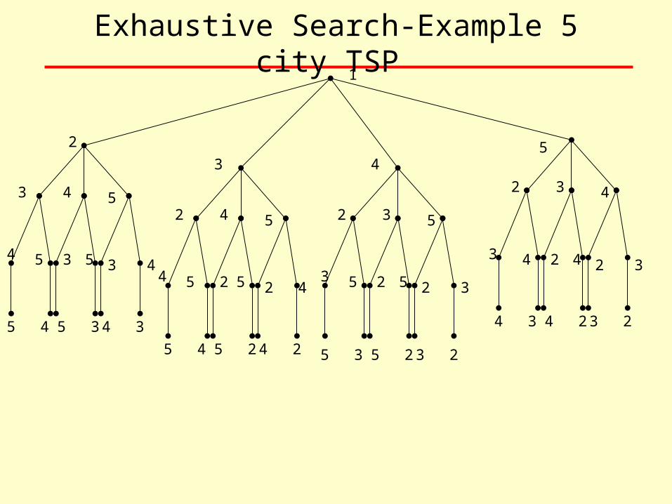
Exhaustive Search-Example 5 city TSP 1

2

3 45

3 4 52 4 5 2 3 5

2 3 4

4 5

5 4 5 3 4 3

5 4 5 2 4 2 5 3 5 2 3 2

4 3 4 2 3 2

3 5 3 44 5 2 5 2 4

3 5 2 5 2 3

3 4 2 4 2 3

Exhaustive Search -Example 5 city TSP 1

2

3 45

3 4 52 4 5 2 3 5

2 3 4

4 5

5 4 5 3 4 3

5 4 5 2 4 2 5 3 5 2 3 2

4 3 4 2 3 2

3 5 3 44 5 2 5 2 4

3 5 2 5 2 3

3 4 2 4 2 3

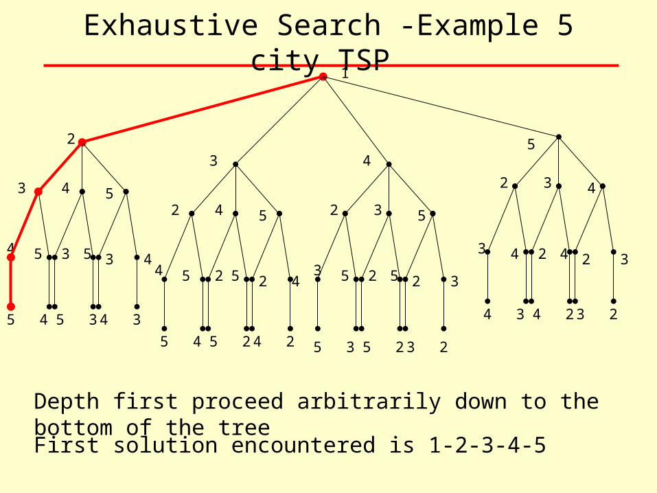
Depth first proceed arbitrarily down to the bottom of the tree

First solution encountered is 1-2-3-4-5

Exhaustive Search -Example 5 city TSP 1

2

3 45

3 4 52 4 5 2 3 5

2 3 4

4 5

5 4 5 3 4 3

5 4 5 2 4 2 5 3 5 2 3 2

4 3 4 2 3 2

3 5 3 44 5 2 5 2 4

3 5 2 5 2 3

3 4 2 4 2 3

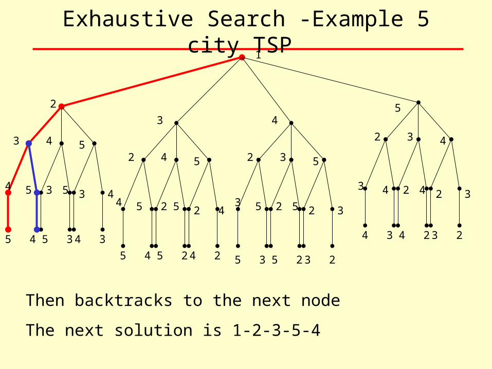
Then backtracks to the next node

The next solution is 1-2-3-5-4

Exhaustive Search -Example 5 city TSP 1

2

3 45

3 4 52 4 5 2 3 5

2 3 4

4 5

5 4 5 3 4 3

5 4 5 2 4 2 5 3 5 2 3 2

4 3 4 2 3 2

3 5 3 44 5 2 5 2 4

3 5 2 5 2 3

3 4 2 4 2 3

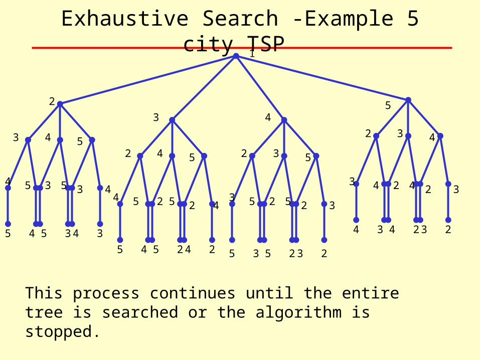
This process continues until the entire tree is searched or the algorithm is stopped.

Depth-First Search

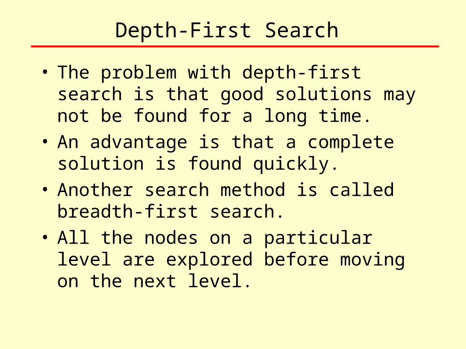
• The problem with depth-first search is that good solutions may not be found for a long time.

• An advantage is that a complete solution is found quickly.

• Another search method is called breadth-first search.

• All the nodes on a particular level are explored before moving on the next level.

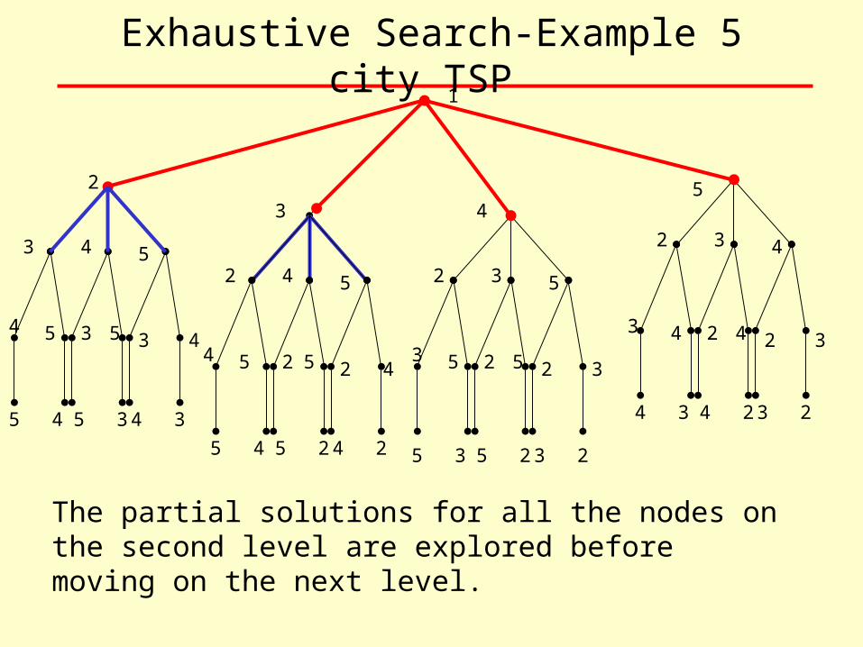
Exhaustive Search-Example 5 city TSP 1

2

3 45

3 4 52 4 5 2 3 5

2 3 4

4 5

5 4 5 3 4 3

5 4 5 2 4 2 5 3 5 2 3 2

4 3 4 2 3 2

3 5 3 44 5 2 5 2 4

3 5 2 5 2 3

3 4 2 4 2 3

The partial solutions for all the nodes on the second level are explored before moving on the next level.

Breadth-First Search

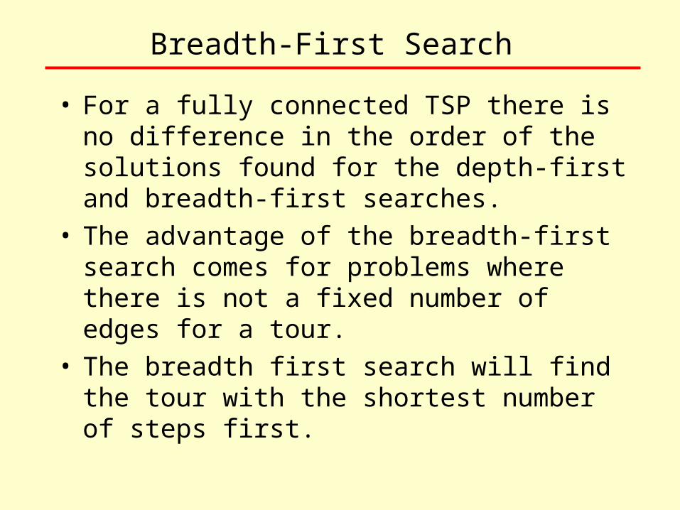
• For a fully connected TSP there is no difference in the order of the solutions found for the depth-first and breadth-first searches.

• The advantage of the breadth-first search comes for problems where there is not a fixed number of edges for a tour.

• The breadth first search will find the tour with the shortest number of steps first.

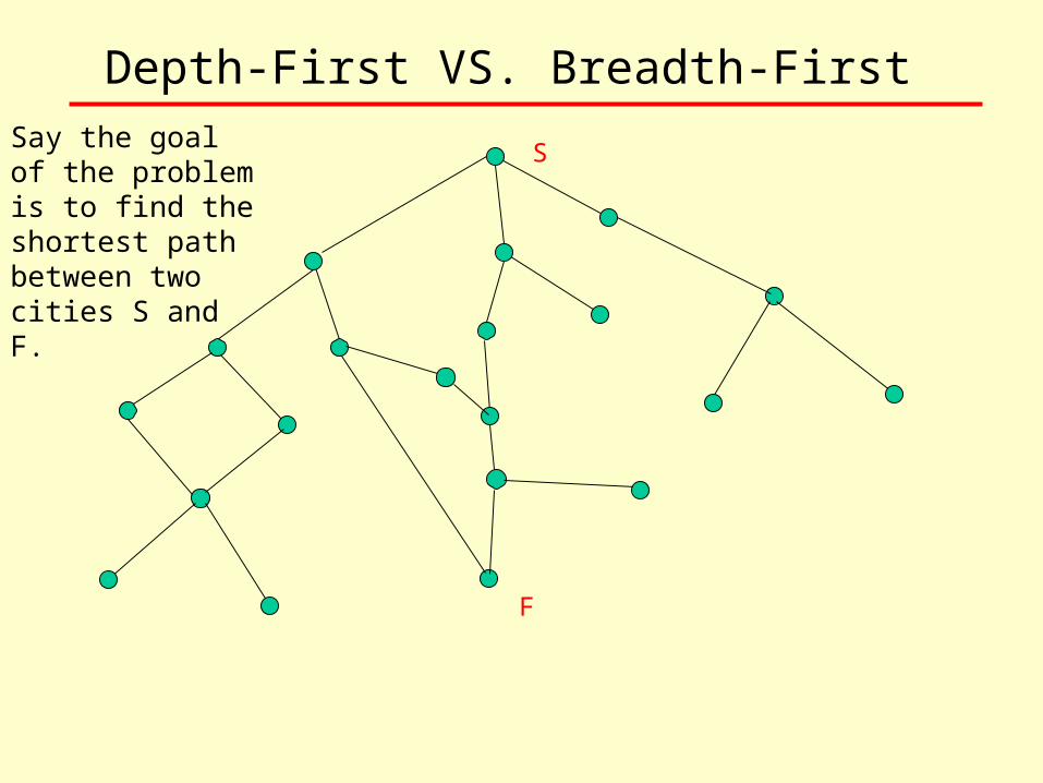
Depth-First VS. Breadth-First Say the goal of the problem is to find the shortest path between two cities S and F.

S

F

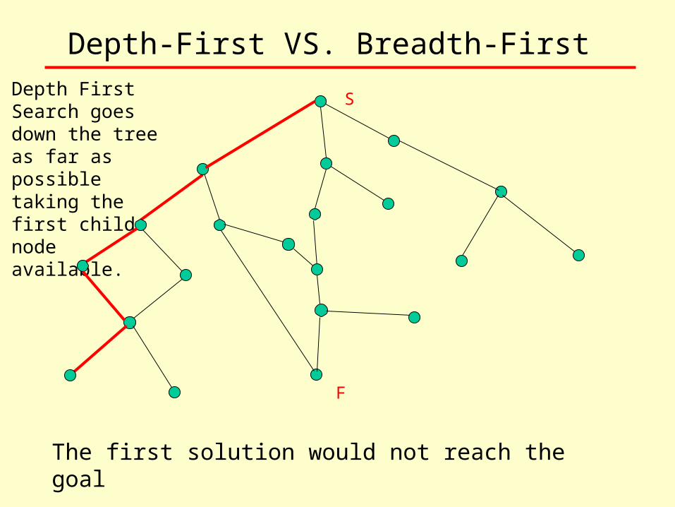
Depth-First VS. Breadth-First Depth First Search goes down the tree as far as possible taking the first child node available.

S

F

The first solution would not reach the goal

Depth-First VS. Breadth-First Breadth first search would search each level at a time

S

F

Best-first Search

• Another option is to try to order the available nodes based on some heuristic that corresponds to our expectations on what we will find when we get to the lowest level of the search.

• We want to first search the nodes that offer the best chance of finding a good solution.

• This is equivalent to using a greedy algorithm first to try to find a good solution quickly so that more solution will be eliminated when we calculate the lower bound.

• This is called ‘best-first-search’.

Best-First Search

• Best first search is a little like hill climbing, in that it uses an evaluation function and always chooses the next node to be that with the best score.

• However, it is exhaustive, in that it should eventually try all possible paths.

• Instead of taking the first node like depth-first-search it will take the best node off, ie the node with the best score.

• The score is computed by estimating the cost to the goal (i.e the cost from the current node to the end of the tour) and adding to that the cost to the current state.

Branch and Bound

• The main differences between the best-first algorithm and the depth-first algorithm are:

• Best first explored the most promising next node whereas depth first goes as deep as possible in a arbitrary pattern.

• Best-first search uses a heuristic that provides a merit value for each node whereas depth first does not.

Branch and Bound

• The quality of the heuristic determines the efficiency of the best-search algorithm.

• In the process of evaluating a partially constructed solution q we have to take into account 2 components

1. The merit of the decisions already made, c(q).

2. The potential inherent to the remaining decisions, h’(q).

The evaluation function for the partial solution q is:

f’ (q)=c(q)+h’ (q)

Branch and Bound

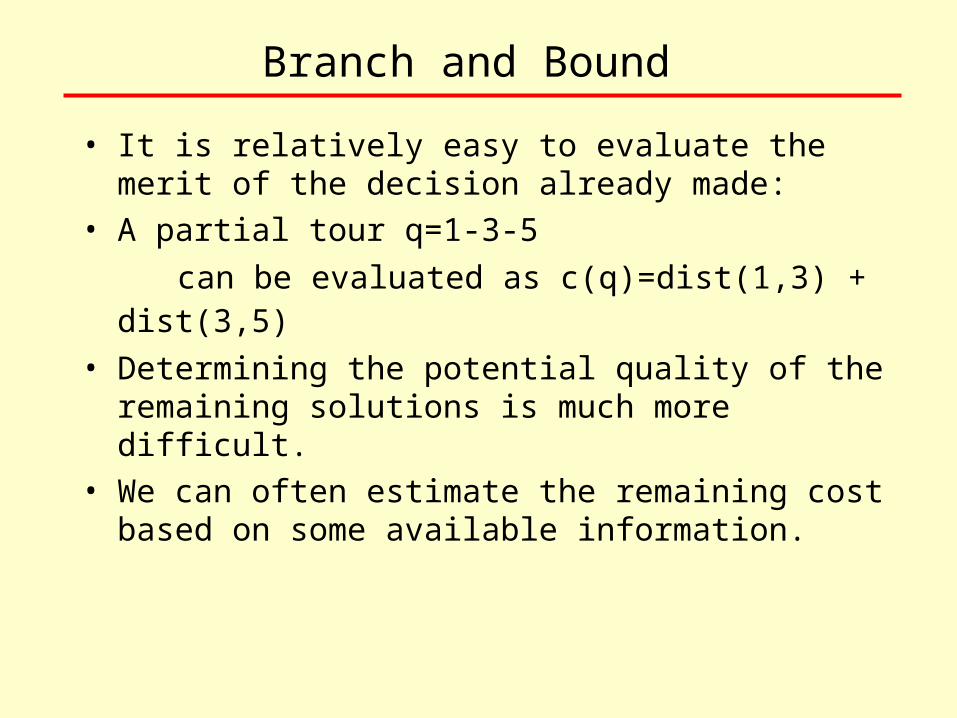
• It is relatively easy to evaluate the merit of the decision already made:

• A partial tour q=1-3-5

can be evaluated as c(q)=dist(1,3) + dist(3,5) • Determining the potential quality of the remaining

solutions is much more difficult.

• We can often estimate the remaining cost based on some available information.

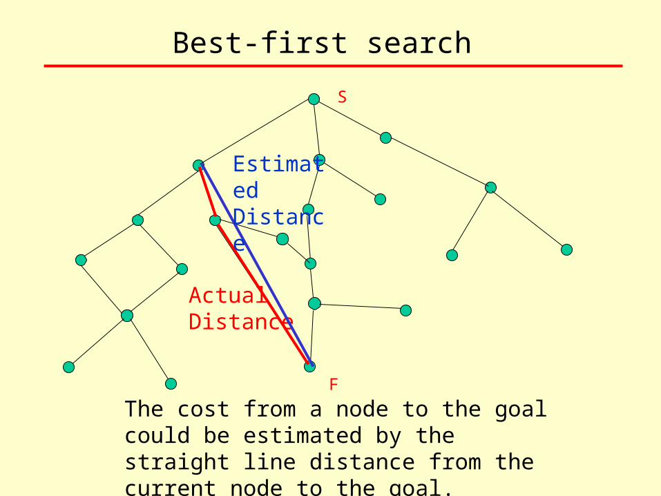
Best-first search

S

F

The cost from a node to the goal could be estimated by the straight line distance from the current node to the goal.

Actual Distance

Estimated Distance

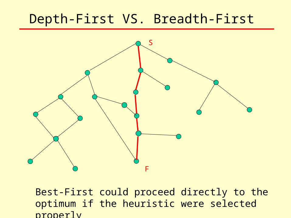
Depth-First VS. Breadth-First

S

F

Best-First could proceed directly to the optimum if the heuristic were selected properly

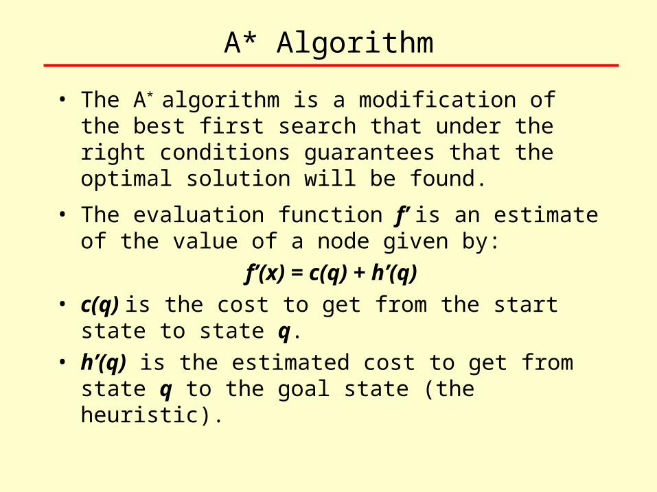
A* Algorithm

• The A* algorithm is a modification of the best first search that under the right conditions guarantees that the optimal solution will be found.

• The evaluation function f’ is an estimate of the value of a node given by:

f’(x) = c(q) + h’(q)• c(q) is the cost to get from the start state to state q.

• h’(q) is the estimated cost to get from state q to the goal state (the heuristic).

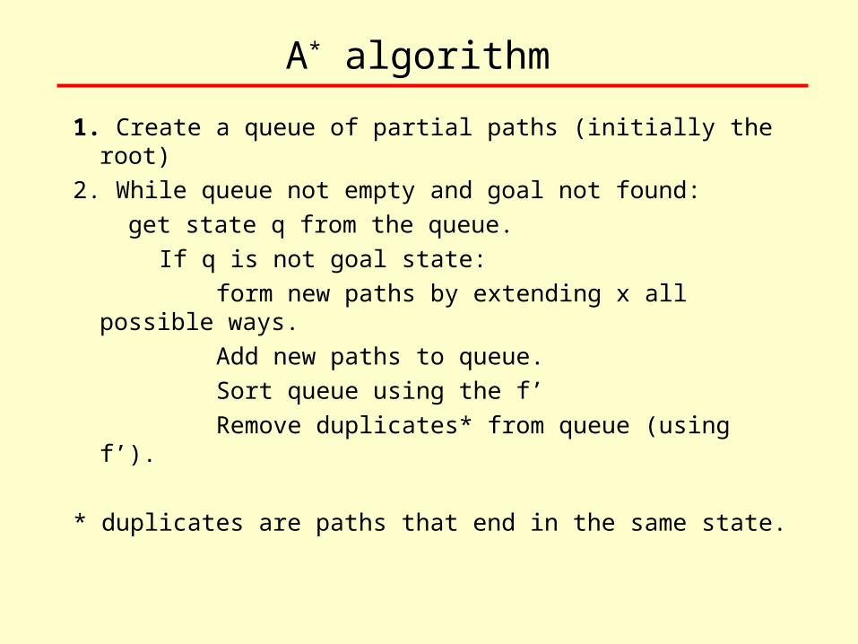
A* algorithm

1. Create a queue of partial paths (initially the root)

2. While queue not empty and goal not found: get state q from the queue.

If q is not goal state: form new paths by extending x all possible

ways. Add new paths to queue. Sort queue using the f’ Remove duplicates* from queue (using f’).

* duplicates are paths that end in the same state.

A* Optimality and Completeness • If the heuristic function h’ is admissible the algorithm will

find the cheapest path to the solution in the minimum number of steps.

• An admissible heuristic is one that never overestimates the cost of getting from a state to the goal state.

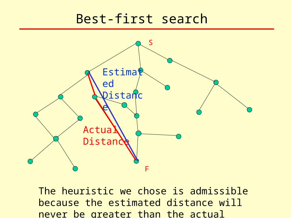
Best-first search

S

F

The heuristic we chose is admissible because the estimated distance will never be greater than the actual distance.

Actual Distance

Estimated Distance

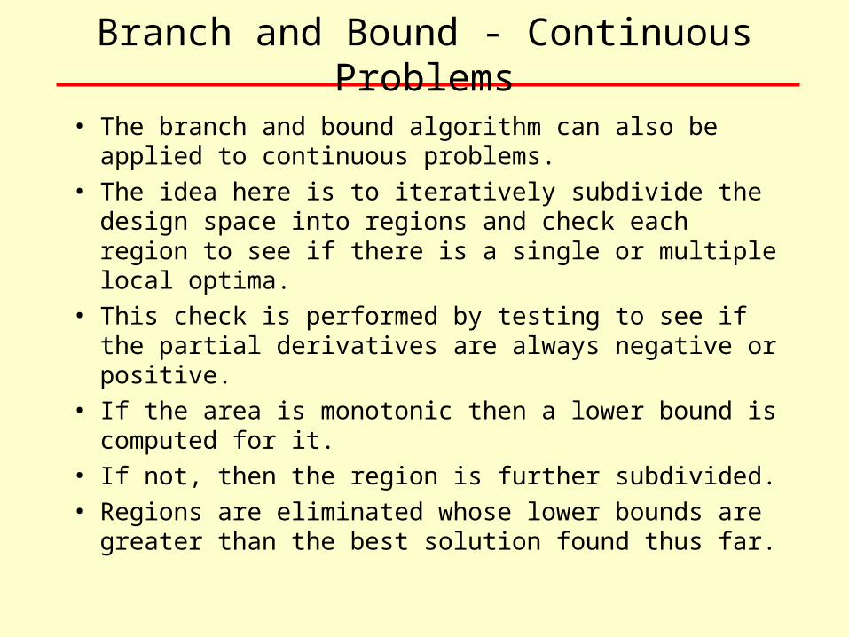
Branch and Bound - Continuous Problems

• The branch and bound algorithm can also be applied to continuous problems.

• The idea here is to iteratively subdivide the design space into regions and check each region to see if there is a single or multiple local optima.

• This check is performed by testing to see if the partial derivatives are always negative or positive.

• If the area is monotonic then a lower bound is computed for it.

• If not, then the region is further subdivided.

• Regions are eliminated whose lower bounds are greater than the best solution found thus far.

Branch and Bound

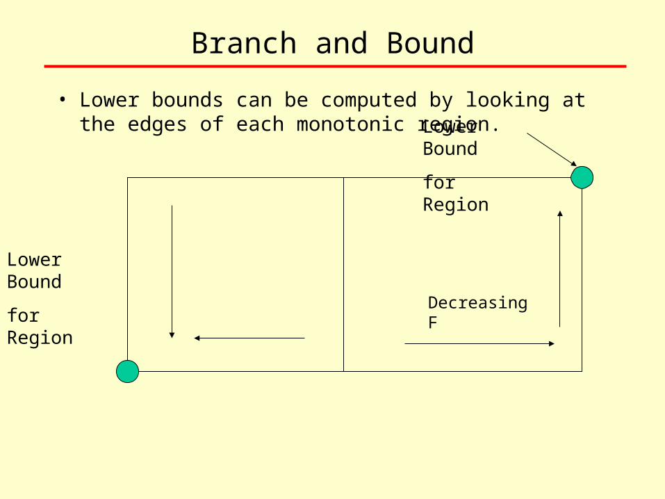
• Lower bounds can be computed by looking at the edges of each monotonic region.

Decreasing F

Lower Bound

for Region

Lower Bound

for Region

Branch and Bound

• There are many variants of this generic branch and bound algorithm

– Interval analysis can be used to determine the bounds where the calculations are performed on intervals instead of on real number

– A stochastic version of the algorithm calculates f at random points to determine a lower bound.

• We will go into the application of Branch and Bound to continuous problems in more detail next lecture