MAE 552 – Heuristic Optimization

Lecture 26

April 1, 2002

Topic:Branch and Bound

Parallel and Distributed Branch-and-Bound/A* Algorithms

A Branch-and-Bound Algorithm for the Quadratic Assignment Problem

Branch and Bound

• We have seen this semester that the size of real-world problems grows very large as the number of design variables increases.

• Recall that there are (n-1)!/2 different solutions for the Travelling Salesman Problem (TSP).

• Exhaustive search is impractical when n>20

• It would be helpful of we could reduce the size of the search space where we know the optimum solution will not exist.

Branch and Bound

• Branch and Bound works on the idea of successively partitioning the design space.

• 1st we need some means on determining a lower bound on the cost of any particular solution.

• A lower bound on a solution means the solution will cost at least the value of this lower bound.

• If we are maximizing the we need to find an upper bound on a solution - a value which this solution cannot exceed

Branch and Bound

• For minimization– If we have a solution 1 with a cost c– AND we know that another solution 2 has

lower bound that is greater than c– THEN we do not need to evaluate 2 because

we know that 2 will exceed 1.

Branch and Bound

• For maximization– If we have a solution 1 with a cost c– AND we know that another solution 2 has

upper bound that is less than c– THEN we do not need to evaluate 2 because

we know that 2 will never exceed 1.

Branch and Bound

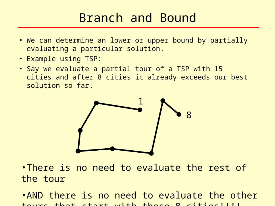
• We can determine an lower or upper bound by partially evaluating a particular solution.

• Example using TSP:• Say we evaluate a partial tour of a TSP with 15 cities and after 8

cities it already exceeds our best solution so far.

1

8

•There is no need to evaluate the rest of the tour

•AND there is no need to evaluate the other tours that start with those 8 cities!!!!

Branch and Bound

• The design space can be organized in a tree structure

• The branch and bound prunes away branches that are not of interest.

• The design space of the TSP can be organized on the basis of whether or not edge (1 2) occurs in the solution.

• It can be further divided into branches where edge (2 3) appears and so forth.

• Consider the search space of a 5 city TSP with 12 total solutions

Branch and Bound

SUnderline means edge not present in solution

(1 2) (1 2)

(1 2)(2 3)

(1 2)(2 3)

(1 2)(2 3)(3 4)

(1 2)(2 3)(3 4)

1-2-3-4-5 1-2-3-5-4

(1 2)(2 3)

(1 2)(2 3)(3 4)

(1 2)(2 3)

(1 2)(2 3)(3 4)

(1 2)(2 3)(3 4)

(1 2)(2 3)(3 4)(1 5)

1-2-4-3-5

(1 2)(2 3)(3 4)(1 5)

1-2-4-5-3

(1 2)(2 3)

(1 2)(2 3)(3 4)

(1 2)(2 3)(3 4)

(1 2)(2 3)(3 4)

(1 2)(2 3)(3 4)

1-3-5-2-41-5-2-4-31-5-2-3-4

(1 2)(2 3)(3 4)(2 5)

(1 2)(2 3)(3 4)(2 5)

1-3-2-5-4

Branch and Bound

• Suppose the cost can for travelling between cities is described by the following cost matrix.

•Each entry is the cost of travelling from a city in the ith row to one in the jth column.

•The zeros down the diagonal indicate that you cannot travel from a city to itself

C =

0 7 12 8 117 0 10 7 13

12 10 0 9 128 7 9 0 10

11 13 12 10 0

Branch and Bound

• Given the search tree we need a heuristic for estimation a lower bound on the cost of any final solution, or even any solution containing a particular node (i.e. city)

• If the lower bound is higher than the best solution we have found so far, we can keep looking without having to actually compute its final cost.

Branch and Bound

• Here is a simple but not very effectual way to compute a lower bound for a tour.

• Consider a complete solution for the TSP.

• Every tour comprises 2 adjacent edges for every city, one edge enters the city, one edge goes on to the next city.

• If we select the two shortest edges that are connected to each city and take the sum of these edges divided by 2 we will obtain a lower bound.

• We could not possibly do better because this selects the very best edges for all the cities.

Branch and Bound

• With respect to the cost matrix this turns out to be

[(7+8)+(7+7)+(9+10)+(7+8)+(10+11)]/2=84/2=42

• Note that 7 and 8 in the first parentheses correspond to the lengths of the two shortest edges connected to city 1 whereas the 7 and 7 correspond to the lengths of the two shortest edges connected to city 2 and so on

C =

0 7 12 8 117 0 10 7 13

12 10 0 9 128 7 9 0 10

11 13 12 10 0

Branch and Bound

• At first glance this may seem to be good way find a good solution but it is important to note that determining the lower bound does not specify a solution.

• It is not possible to specify a solution that incorporates all of these shortest edges because it is generally necessary to specify some worse edges to form a legal tour.

Branch and Bound

• Once some edges are specified we can incorporate that information and calculate a lower bound on that partial solution.

• If we knew that edge (2 3) were included but edge (1 2) was not then the lower bound on the partial solution would be:

[(8+11)+(7+10)+(9+10)+(7+8)+(10+11)]/2=45.5

C =

0 7 12 8 117 0 10 7 13

12 10 0 9 128 7 9 0 10

11 13 12 10 0

Branch and Bound

• We can improve the lower bound by including the implied edges or excluding those that cannot occur.

• If we determined that edges (1 2) and (2 4) were included in a tour then we would get a lower bound of 42.

• But with these two edges included we can exclude edge (1 4) which would raise the lower bound to 44.

• If we already have a solution less than 44 then we can eliminate every possible solution containing edges (1 2) and (2 4) WITHOUT EVALUATING THEM.

Branch and Bound

• Exercise: Show that with edges (1 2) and (2 4) included the lower bound is 44.

[( )+( ) + ( ) + ( ) + ( )]/2=C =

0 7 12 8 117 0 10 7 13

12 10 0 9 128 7 9 0 10

11 13 12 10 0

[(7+11)+( 7+7 ) + ( 9+10) + (7+9) + ( 10+11 )]/2=44

Branch and Bound

• Exercise: Find the lower bound with edges (3 5) and (5 1) excluded.

[(7+8)+(7+7) + (9+10) + (7+8) + (10+13)]/2=43

C =

0 7 12 8 117 0 10 7 13

12 10 0 9 128 7 9 0 10

11 13 12 10 0

[( )+( ) + ( ) + ( ) + ( )]/2=

Branch and Bound

• It is important to recognize that is cost time to compute the lower bounds

• The cost of computing the lower bounds has to be made up in the time saved in pruning the tree.

• So we want the best lower bound possible, to ensure efficient pruning.

• This is the subject of much research.

Branch and Bound - Continuous Problems

• The branch and bound algorithm can also be applied to continuous problems.

• The idea here is to iteratively subdivide the design space into regions and check each region to see if there is a single or multiple local optima.

• This check is performed by testing to see if the partial derivatives are always negative or positive.

• If the area is monotonic then a lower bound is computed for it.

• If not, then the region is further subdivided.

• Regions are eliminated whose lower bounds are greater than the best solution found thus far.

Branch and Bound

• Lower bounds can be computed by looking at the edges of each monotonic region.

Decreasing F

Lower Bound

for Region

Lower Bound

for Region

Branch and Bound

• There are many variants of this generic branch and bound algorithm

– Interval analysis can be used to determine the bounds where the calculations are performed on intervals instead of on real number

– A stochastic version of the algorithm calculates f at random points to determine a lower bound.

• We will go into the application of Branch and Bound to continuous problems in more detail next lecture