madoc.bib.uni-mannheim.demadoc.bib.uni-mannheim.de/43855/1/20180119_thesismhess.pdfmadoc.bib.uni-mannheim.de...
TRANSCRIPT

An Enumerative Method for Convex
Programs with Linear Complementarity
ConstraintsAnd Application to the Bilevel Problem of a Forecast Model
for High Complexity Products
Inauguraldissertation
zur Erlangung des akademischen Grades
eines Doktors der Naturwissenschaften
der Universitat Mannheim
vorgelegt von
Dipl. Math. Maximilian Heß
aus Karlsruhe
Mannheim, 2017

ii
Dekan: Dr. Bernd Lubcke, Universitat Mannheim
Referent: Professorin Dr. Simone Gottlich, Universitat Mannheim
Korreferent: Professor Dr. Michael Herty, Universitat Aachen
Tag der mundlichen Prufung: 24. November 2017
iii
Abstract
The increasing variety of high complexity products presents a challenge in ac-
quiring detailed demand forecasts. Against this backdrop, a convex quadratic
parameter dependent forecast model is revisited, which calculates a prognosis
for structural parts based on historical order data. The parameter dependency
inspires a bilevel problem with convex objective function, that allows for the cal-
culation of optimal parameter settings in the forecast model. The bilevel prob-
lem can be formulated as a mathematical problem with equilibrium constraints
(MPEC), which has a convex objective function and linear constraints.
Several new enumerative methods are presented, that find stationary points or
global optima for this problem class. An algorithmic concept shows a recursive
pattern, which finds global optima of a convex objective function on a general
non-convex set defined by a union of polytopes. Inspired by these concepts the
thesis investigates two implementations for MPECs, a search algorithm and a
hybrid algorithm. They incorporate and extend the techniques of the CASET
and BBASET algorithm by Judice et al. [35, 34]. In this context, a new approach
is presented that solves the general linear complementarity problem (GLCP), that
arises at new nodes of the BBASET algorithm. This approach uses and extends
an algorithm of Hu et al. [24], that originally solves MPECs with linear objective
function. The new approach works for arbitrary constraint matrices.
Several techniques are investigated for the new enumerative methods, such as
cut generation by linear problems (based on the results of Balas et al. [3]),
as well as different branching strategies [43, 44], lower bound calculation with
the Lagrange function, a new relaxation scheme for the complementary variables
in the search method, and specialized constraints for the bilevel MPEC of the
forecast model. The new methods utilize a solver for convex programs in their
core and are subject to extensive numerical testing. Results are generated for the
demand-forecast-bilevel-problem and instances from a collection of test problems
[70].
The results show that these methods work reliably with the given instances and
can find A-stationary points or local optima of high quality with good perfor-
mance. The global solution method is compared to a commercial MIQP-solver
and outperforms it on two larger instances.

iv
Zusammenfassung
Die hohe Variantenvielfalt komplexer Serienprodukte macht es zunehmend schwieriger
detailerte Bedarfsprognosen zu erstellen. Hierzu wird eine Prognosemethode
vorgestellt und untersucht, welche eine Teilebedarfsermittlung auf der Basis his-
torischer Auftragsdaten durchfuhrt und auf einem parameterabhangigen kon-
vexen quadratisches Problem basiert. Das Modell bildet den Ausgangspunkt
fur ein Bilevel-Problem mit konvexer Zielfunktion, welches zur Ermittlung eines
optimalen Parametervektors dient. Dieses Bilevel-Problem kann als mathema-
tisches Problem mit Gleichgewichtsrestriktionen (MPEC) formuliert werden, die
Zielfunktion des MPECs ist konvex, die Nebenbedingungen sind linear.
Es werden mehrere neue enumerative Methoden prasentiert, welche stationare
Punkte oder globale Optima fur diese Problemklasse liefern. Grundlegend wird
ein algorithmisches Konzept vorgestellt, welches auf einer nicht-konvexen Menge,
die als Vereinigung von Polytopen definiert ist, durch rekursive Aufrufe ein glob-
ales Optimum einer konvexen Zielfunktion findet. Dieses Konzept inspiriert zwei
Algorithm fur den Fall der vorliegenden MPECs, einen Such-Algorithmus und
einen hybriden Algorithmus. Diese Algorithmen verwenden und erweitern die
Resultate des CASET und BBASET Algorithmus von Judice et al. [35, 34] und
hierbei wird außerdem ein neuer Ansatz prasentiert, welcher die allgemeinen lin-
earen Komplementaritatsprobleme (GLCPs) lost, die im BBASET-Algorithmus
bei der Generation neuer Knoten entstehen. Der Ansatz basiert auf einem Algo-
rithmus von Hu et al. [24], welcher ursprunglich MPECs mit linearer Zielfunktion
lost und in diesem Zusammenhang adaptiert und erweitert wird. Die Methodik
funktioniert mit beliebigen Systemen linearer Nebenbedingungen.
Fur die neuen enumerativen Methoden werden außerdem zusatzliche Techniken
untersucht, wie zum Beispiel die Erzeugung von Schnittebenen durch die Losung
linearer Probleme (basierend auf den Untersuchungen von Balas et al. [3]),
sowie verschiedene Verzweigungsstrategien [43, 44], die Berechnung von Unter-
schranken mit der Lagrange-Funktion, ein neues Relaxierungs-Schema fur die
komplementaren Variablen (welches im Such-Algorithmus zum Einsatz kommt)
und die Generation spezieller Nebenbedingungen fur das Bilevel-MPEC des Prog-
nose Problems. Die neuen Methoden arbeiten im Kern mit einem Loser fur
konvexe Probleme und wurden ausgiebig numerisch getestet, sowohl mit den In-
stanzen des Bilevel-Prognose-Problems als auch mit Instanzen die in einer Samm-

v
lung von Testproblemen zu finden sind [70].
Die Ergebnisse zeigen, dass die Methoden die vorliegenden Instanzen zuverlassig
bearbeiten konnen und mit guter Performance A-stationare Punkte oder lokale
Optima mit niedrigem Zielfunktionswert liefern. Die globalen Methoden werden
bei den Tests mit einem kommerziellen MIQP-Loser verglichen und weisen bei
zwei großeren Instanzen eine bessere Performance auf.

Contents
List of Figures . . . . . . . . . . . . . . . . . . . . . . . . . . . . . . . . ix
List of Tables . . . . . . . . . . . . . . . . . . . . . . . . . . . . . . . . . x
1. Introduction . . . . . . . . . . . . . . . . . . . . . . . . . . . . . . . 1
2. Stationary Concepts and Solution Methods for MPECs . . . . 6
2.1. Common Stationary Conditions and Constraint Qualifications . . 6
2.2. Stationary Concepts for MPECs . . . . . . . . . . . . . . . . . . 9
2.3. Solution Algorithms for MPECs . . . . . . . . . . . . . . . . . . . 21
2.4. Outlook . . . . . . . . . . . . . . . . . . . . . . . . . . . . . . . . 23
3. The Reweighting Problem . . . . . . . . . . . . . . . . . . . . . . . 24
3.2. The Demand Forecast Model . . . . . . . . . . . . . . . . . . . . 26
3.3. Continuity of the Solution Map and Variational Inequalities . . . 34
3.4. The Reweighting Bilevel Problem . . . . . . . . . . . . . . . . . . 38
3.4.1. The Practical Reweighting Bilevel Problem . . . . . . . . . 42
3.5. An Algorithmic Concept . . . . . . . . . . . . . . . . . . . . . . . 43
4. CASET and BBASET . . . . . . . . . . . . . . . . . . . . . . . . . 46
4.1. CASET . . . . . . . . . . . . . . . . . . . . . . . . . . . . . . . . 46
4.2. BBASSET . . . . . . . . . . . . . . . . . . . . . . . . . . . . . . 53
4.2.1. Lower Bounds . . . . . . . . . . . . . . . . . . . . . . . . . . 56
4.2.2. Algorithm . . . . . . . . . . . . . . . . . . . . . . . . . . . . 56
4.2.3. Disjunctive Cuts . . . . . . . . . . . . . . . . . . . . . . . . 58
4.2.4. Feasible Points . . . . . . . . . . . . . . . . . . . . . . . . . 60
4.3. Performing CASET as a Chain of Convex Programs . . . . . . . 61
4.3.1. Anticycling and B-Stationarity . . . . . . . . . . . . . . . . 65
4.4. Methodological Outlook . . . . . . . . . . . . . . . . . . . . . . . 67
vi

Contents vii
5. A Modification of the Algorithm of Hu et al. . . . . . . . . . . . 68
5.1. The General Linear Complementarity Problem . . . . . . . . . . 69
5.1.1. A Pivoting Algorithm for LPCCs . . . . . . . . . . . . . . . 74
5.2. The Method of Hu et al. . . . . . . . . . . . . . . . . . . . . . . . 76
5.2.1. Extreme Point and Ray Cuts . . . . . . . . . . . . . . . . . 80
5.2.2. Sparsification Procedure . . . . . . . . . . . . . . . . . . . . 81
5.2.3. Main Algorithm . . . . . . . . . . . . . . . . . . . . . . . . 83
5.3. Adaptation and Application of the Method . . . . . . . . . . . . 84
5.3.1. The Algorithm . . . . . . . . . . . . . . . . . . . . . . . . . 88
5.3.2. Partial Feasibility . . . . . . . . . . . . . . . . . . . . . . . . 89
5.3.3. Intermediate Computational Results . . . . . . . . . . . . . 92
5.3.4. Conclusion . . . . . . . . . . . . . . . . . . . . . . . . . . . 96
6. Lower Bounds from Weak Duality . . . . . . . . . . . . . . . . . 97
6.2. Remarks on Convex Analysis . . . . . . . . . . . . . . . . . . . . 99
6.3. Application . . . . . . . . . . . . . . . . . . . . . . . . . . . . . . 103
6.4. Conclusion . . . . . . . . . . . . . . . . . . . . . . . . . . . . . . 106
7. A Hybrid branch-and-bound Algorithm for Convex
Programs with Linear Complementarity Constraints . . . . . . 107
7.1. An Algorithm for Non-Convex Polyhedral Sets . . . . . . . . . . 107
7.1.1. Algorithm Convergence . . . . . . . . . . . . . . . . . . . . 117
7.2. Application to the Reweighting Bilevel Problem . . . . . . . . . . 120
7.3. Hybrid Algorithm - Search Phase . . . . . . . . . . . . . . . . . . 123
7.3.1. Implementation . . . . . . . . . . . . . . . . . . . . . . . . . 124
7.4. Disjunctive Cuts . . . . . . . . . . . . . . . . . . . . . . . . . . . 130
7.5. Constraints based on the Objective Function Gradient . . . . . . 132
7.6. Hybrid Algorithm - Global Optimality . . . . . . . . . . . . . . . 133
7.6.1. Branching Strategies . . . . . . . . . . . . . . . . . . . . . . 133
7.6.2. Application to the Reweighting Bilevel Problem . . . . . . . 138
7.6.3. A Modification of the BBASET Method . . . . . . . . . . . 144
7.6.4. The Method of Hu et al. and Lagrange Lower Bounds . . . 144
7.6.5. The Hybrid Algorithm . . . . . . . . . . . . . . . . . . . . . 147

Contents viii
8. Computational Results . . . . . . . . . . . . . . . . . . . . . . . . . 152
8.1. Components . . . . . . . . . . . . . . . . . . . . . . . . . . . . . 152
8.2. Disclaimer and Technical Details . . . . . . . . . . . . . . . . . . 154
8.3. Data and Problem Instances . . . . . . . . . . . . . . . . . . . . . 155
8.3.1. Reweighting Bilevel Instances . . . . . . . . . . . . . . . . . 155
8.3.2. QPEC Problems . . . . . . . . . . . . . . . . . . . . . . . . 156
8.4. Search Phase . . . . . . . . . . . . . . . . . . . . . . . . . . . . . 159
8.4.1. QPEC Problems . . . . . . . . . . . . . . . . . . . . . . . . 159
8.5. Global Optima . . . . . . . . . . . . . . . . . . . . . . . . . . . . 162
8.5.1. QPEC Problems . . . . . . . . . . . . . . . . . . . . . . . . 162
8.5.2. Reweighting Bilevel Instances . . . . . . . . . . . . . . . . . 163
8.6. Conclusion . . . . . . . . . . . . . . . . . . . . . . . . . . . . . . 168
Bibliography . . . . . . . . . . . . . . . . . . . . . . . . . . . . . . . . . 170
Appendix . . . . . . . . . . . . . . . . . . . . . . . . . . . . . . . . . . . 177
A. Computational Results . . . . . . . . . . . . . . . . . . . . . . . . . 178
A.1. Search Phase Iterations . . . . . . . . . . . . . . . . . . . . . . . 178
A.2. CPLEX MIQP Solver with MIP-Starts provided by the Hybrid
Algorithm in Search Mode . . . . . . . . . . . . . . . . . . . . . . 178
A.3. The Hybrid Algorithm on Global Optimality . . . . . . . . . . . 184
List of Figures
1.1. Chapter Overview . . . . . . . . . . . . . . . . . . . . . . . . . . . 4
2.1. MPEC Stationary Concepts (Example 2.1) . . . . . . . . . . . . . 14
3.1. Algorithmic Concept for the Reweighting Bilevel Problem . . . . . 45
4.1. Illustration of the CASET Algorithm . . . . . . . . . . . . . . . . 47
4.2. Objective Function of (4.21) . . . . . . . . . . . . . . . . . . . . . 53
4.3. Illustration of the BBASET Algorithm for λζi , λζj , λ
wk ă 0 . . . . . . 55
6.1. Geometric Argument in Theorem 6.2 . . . . . . . . . . . . . . . . 102
7.1. Recursive Algorithm Variant 1 . . . . . . . . . . . . . . . . . . . . 114
7.2. Recursive Algorithm Variant 2 . . . . . . . . . . . . . . . . . . . . 114
7.3. Recursive Algorithm Variant 3 . . . . . . . . . . . . . . . . . . . . 116
7.4. Feasible Set of an Exemplary Reweighting Bilevel Problem with
x P R2 . . . . . . . . . . . . . . . . . . . . . . . . . . . . . . . . . 122
7.5. Feasible Set of an Exemplary Reweighting Bilevel Problem with
Two Connected Components for pXzpi`qq X Pi` . . . . . . . . . . 122
7.6. Simplified Diagram of Algorithm 14 . . . . . . . . . . . . . . . . . 130
8.1. Hybrid Algorithm in Search Mode, qpec-100-1 (left), qpec-100-2
(right) . . . . . . . . . . . . . . . . . . . . . . . . . . . . . . . . . 160
8.2. Hybrid Algorithm in Search Mode, qpec-100-3 (left), qpec-100-4
(right) . . . . . . . . . . . . . . . . . . . . . . . . . . . . . . . . . 160
8.3. Hybrid Algorithm in Search Mode, qpec-200-1 (left), qpec-200-2
(right) . . . . . . . . . . . . . . . . . . . . . . . . . . . . . . . . . 160
8.4. Hybrid Algorithm in Search Mode, qpec-200-3 (left), qpec-200-4
(right) . . . . . . . . . . . . . . . . . . . . . . . . . . . . . . . . . 161
ix
List of Tables
3.1. Format Sample of the Technical Documentation . . . . . . . . . 25
3.2. A Randomized Data Sample . . . . . . . . . . . . . . . . . . . . 31
5.1. Performance of Algorithm 8 on a small Test Set . . . . . . . . . 95
5.2. Performance of the Cplex MIQP Solver on the same Test Set . . 96
8.1. Objective Function Characteristics of the Reweighting Bilevel
Instances . . . . . . . . . . . . . . . . . . . . . . . . . . . . . . . 156
8.2. Characteristics of the QPEC Test Instances . . . . . . . . . . . . 158
8.3. Computational Reference: l1 Elastic Interior Point Mehod . . . . 161
8.4. Computational Reference: Cplex 12.1 MIQP-Solver . . . . . . . 162
8.5. Performance Indicators . . . . . . . . . . . . . . . . . . . . . . . 162
8.6. Performance of Most Infeasible Branching by Repeated Calls to
the Cplex QP Solver . . . . . . . . . . . . . . . . . . . . . . . . . 163
8.7. Cplex MIQP Solver in Classic Branch-and-Bound Mode with
MIP-Starts provided by the Hybrid Algorithm in Search Mode . 164
8.8. Cplex MIQP Solver in Classic Branch-and-Bound Mode with
MIP-Starts provided by the Hybrid Algorithm in Search Mode . 164
8.9. Hybrid Algorithm compared to Cplex MIQP Solver on Global
Optima for the Reweighting Bilevel MPEC . . . . . . . . . . . . 166
8.10. Hybrid Algorithm on the Reweighting Bilevel MPEC - Data Set 1 167
8.11. Upper Level Objective of the Lower Level Solution before and
after the Bilevel Optimization . . . . . . . . . . . . . . . . . . . 167
A.1. Iterations of the Hybrid Algorithm in Search Mode Part 1 on
QPEC Problems . . . . . . . . . . . . . . . . . . . . . . . . . . . 179
A.2. Iterations of the Hybrid Algorithm in Search Mode Part 2 on
QPEC Problems . . . . . . . . . . . . . . . . . . . . . . . . . . . 180
x
List of Tables xi
A.3. CPLEX MIQP Solver in Classic Branch-and-Bound Mode with
MIP-Starts provided by Hybrid Algorithm in Search Mode . . . 181
A.4. CPLEX MIQP Solver in Dynamic Search Mode with
MIP-Starts provided by the Hybrid Algorithm in Search Mode . 182
A.5. CPLEX MIQP Solver in Dynamic Search Mode with
MIP-Starts provided by the Hybrid Algorithm in Search Mode . 183
A.6. Data Set 2 - s “ 20: Hybrid Algorithm on the Proof of Global
Optimality . . . . . . . . . . . . . . . . . . . . . . . . . . . . . . 185
A.7. Data Set 2 - s “ 50: Hybrid Algorithm on the Proof of Global
Optimality . . . . . . . . . . . . . . . . . . . . . . . . . . . . . . 186
A.8. Data Set 3: Hybrid Algorithm on the Proof of Global Optimality 187
A.9. Data Set 4 - s “ 20: Hybrid Algorithm on the Proof of Global
Optimality . . . . . . . . . . . . . . . . . . . . . . . . . . . . . . 188
A.10. Data Set 4 - s “ 40: Hybrid Algorithm on the Proof of Global
Optimality . . . . . . . . . . . . . . . . . . . . . . . . . . . . . . 189

1. Introduction
In 2016 the Organization of Motor Vehicle Manufacturers (OICA) reported a pro-
duction of over 94 million vehicles world wide, of which 60 million were passenger
cars [73].
“Building 60 million vehicles requires the employment of about 9 million
people directly in making the vehicles and the parts that go into them.
This is over 5 percent of the world’s total manufacturing employment.”
– OICA [73]
As one of the main contributors to the global economy, the automotive industry
has been widely affected by the advances in digital technologies and the infor-
mation revolution. Concepts in mobility and transportation are continuously
evolving with the rise of new inventions. But it is not only the manufactured ve-
hicle itself that has been influenced by such developments. As customer demands
adjust to a world of e-commerce and digital retail, the area of product customiza-
tion becomes more and more important [9]. In the context of a make-to-order
manufacturing process, this leads to demanding challenges in terms of marketing
and sales [38, 50, 67]. Against this backdrop, the availability of detailed demand
forecasts has been shown to be of vital importance.
This research was inspired by a mathematical model for structural part demand
forecasts, and its basis was provided by one of the global players in the premium
automotive sector, the Mercedes-Benz R© division of Daimler AG. The mathemati-
cal model is multicriterial [16] as it merges the information of historical customer
orders and future demand forecasts. The solution to this problem is always
uniquely determined, but it depends on a specific set of parameters.
The primary motivation behind this work is to investigate parameter settings of
the forecast model that provide optimal results in a number of training scenar-
1

1.1. Introduction 2
ios. The question leads to a multilayered problem structure, which can then be
formulated as a mathematical problem with equilibrium constraints (MPEC).
MPECs
MPECs have been an active field of research for several years [68, 74, 63, 33,
14]. Their origin in mathematical optimization goes back to researchers such as
Cournot, Stackelberg and Nash, and they have been subject to research by many
authors to this day.
Stackelberg introduces a problem for a market situation where two participants
interact by deciding on individual strategies [69]. They are denoted as the leader
and the follower. In their economical environment they supply the same type of
product, forming the constellation of a duopoly. The key aspect in this model
is that the leader can anticipate the decision of the follower, which is optimal in
the follower’s corresponding perspective. This is an extension to the model of
Cournot, which was introduced earlier and provides a foundation for the work of
Stackelberg. In Cournot’s model both participants are equal and their decisions
are both based on the best-answer principle. Stackelberg’s model entitles the
leader to optimize his own profit by selecting a strategy according to the follower’s
anticipated decision, and leads to a multilevel situation which is sometimes called
a Stackelberg game.
As a breakthrough in Economics, Nash’s research on noncooperative games fol-
lowed the results of Stackelberg’s publication. The Nash-Cournot equilibrium
[58] denotes the situation where among several players that compete simultane-
ously, none of them can increase their profit by a change of strategy under the
assumption that all the other players will keep their selected strategy at the same
time.
Hierarchical structures, as in the Stackelberg game, are the entry point to bilevel
problems [15, 4]. In terms of mathematical optimization, this leads to the question
of characterizing optimal points on the follower’s level. Common principles such
as the Karush-Kuhn-Tucker conditions can be used under certain assumptions
and lead to the element of equilibrium constraints.
A general equilibrium constraint for two real valued functions G and H is satisfied

1.1. Introduction 3
at a point x if
Gpxq ě 0, Hpxq ě 0, GpxqHpxq “ 0. (1.1)
Within the scope of this work a number of solution techniques that are related
to MPECs with linear complementarity constraints are investigated. The main
achievement is the development of a hybrid solution algorithm and its application.
Numerical experiments are conducted essentially with the data instances of the
automotive industrial application, but also with data instances that are publicly
available.
Structure of this Work
The final hybrid algorithm is a framework that connects different methodologies
in a branch-and-bound environment. The theory behind the individual compo-
nents will be introduced successively. The hybrid algorithm will be presented in
its entirety in chapter 7.
In chapter 2 a range of common concepts that help to characterize stationary
conditions for the feasible points of an MPEC is introduced and investigated
[74, 49, 20, 62]. Difficulties for common solution algorithms are mentioned. These
are due to the lack of stationary conditions, such as the Mangasarian-Fromovitz
constraint qualification [22, 59] in MPECs. In this context the chapter will also
develop proofs of two theorems that are known from related literature on the
matter of B-stationarity, strong stationarity and the MPEC linear constraint
qualification.
This is followed by the introduction of the parameter dependent demand forecast
model with application to high complexity products, the so called reweighting
problem. The model is a quadratic problem whose objective function matrix is
positive semi-definite [59]. A new bilevel problem arises when the forecast model
parameters are tuned with a data scenario that simulates a planning situation
and evaluates the outcome. The bilevel problem is formulated as an MPEC
whose feasible set is analyzed in its combinatorial structure. An investigation on
the solution map of the lower level problem allows the possibility to prove the
connectedness of the feasible area of the MPEC [47, 48, 13, 42].
In chapter 4, the CASET algorithm [35] that finds a strongly stationary point in

1.1. Introduction 4
Stationary Concepts and Optimality Conditions for MPECsChapter 2
CASET and BBASETChapter 4
Feasibility ApproachChapter 5
Lagrange Lower
BoundsChapter 6
Hybrid AlgorithmChapter 7
- Search Method
- Global Solution Method
Computational ResultsChapter 8
The Reweighting Bilevel Problem
(Automotive Use Case)Chapter 3
(+ MAC-MPEC
QPEC instances)
Figure 1.1.: Chapter Overview
MPECs with linear complementarity constraints is reviewed. The method can be
extended to find globally optimal solutions in the case of a convex objective func-
tion with a branch-and-bound algorithm [34]. The chapter develops an extension
to this approach for A-stationary points and shows how the CASET algorithm
can be performed by solving a series of convex programs.
Another module of the hybrid algorithm is presented in chapter 5. An algo-
rithm is reviewed that solves MPECs with linear objective function and linear
complementarity constraints by a 0-1 integer based cut generation approach [24].
The method is analyzed and extended to a new adapted version that determines
feasible areas in a general MPEC with linear complementarity constraints.
Standard lower bounds in a branch-and-bound algorithm for MPECs, which are
calculated with a relaxation of the complementarity constraints, can be inefficient
[34, 14, 65, 28, 27]. Chapter 6 establishes a problem that yields a lower bound
generated by the principles of weak duality. The resulting problem is also an
MPEC but avoids some of the complexity by its absence of non-complementarity
constraints. Under certain assumptions it holds that the objective function in
this problem is convex. Furthermore a theorem is presented that characterizes
unbounded directions of a convex function in the context of convex analysis [61].
1.1. Introduction 5
Chapter 7 presents the new hybrid algorithm that uses a combination of the previ-
ously presented elements and investigates their interaction. The hybrid algorithm
focuses on the solution of convex subproblems, and is divided into two stages.
The first stage specializes in finding points with low objective value in an MPEC
with convex objective function and linear complementarity constraints. For this
search algorithm an abstract formulation is given that presents a geometrical
generalization of the principle of the BBASET algorithm for feasible sets defined
by a union of polytopes. The second stage specializes in proving global optimal-
ity. Techniques are included that calculate constraints for the complementary
variables and have proven to be effective in practice.
The last chapter concludes the investigation by a large number of computa-
tional experiments. The commercial solvers Cplex R© and Gurobi R© are imple-
mented in a core unit for the solution of the various convex subproblems. A
highly adjustable branch-and-bound framework with different parameter settings
is wrapped around this core unit. The results of the hybrid solver are compared
to the Cplex MIQP solver for instances of the reweighting bilevel MPEC, and
are also compared to benchmarks of a related article for a number of instances
that are publicly available [29]. They demonstrate that the hybrid algorithm
shows viable performance in some instances. The subroutine that searches for a
stationary point with low objective value performs well on the publicly available
MPEC data. The solution of the bilevel problem in the training scenarios of the
demand forecast model yields an increase of an average of 18% for the quality of
the forecast.

2. Stationary Concepts and Solution Methods
for MPECs
We begin by introducing common stationary concepts and optimality conditions
for general optimization problems, followed by specialized versions for the case of
mathematical problems with equilibrium constraints (MPECs). The last section
presents a list of references for a number of selected articles on the topic of solution
methods and related results.
2.1. Common Stationary Conditions and Constraint
Qualifications
The most basic concepts of stationary conditions and constraint qualifications
from general optimization are introduced briefly. One of the most valuable as-
pects is the existence of multipliers at local optimal points, and in return the
characterization of stationary points by the existence of multipliers. This princi-
ple will be extended to the concept of MPECs in the next section.
A point is locally optimal if no descent is possible in the feasible part of an
environment around this point, which is arbitrarily small. The characterization
of feasible directions, which are considered around a feasible point, is achieved
by introducing the tangent cone.
2.1 Definition (Tangent Cone, [22] def. 2.28, def. 2.31, [59] 12.2) The
tangent cone of X at x P X is defined by
TXpxq :“ td | DpxkqkPN Ď X, DptkqkPN P R, tk Ó 0 : xk Ñ x and pxk ´ xq{tk Ñ du.
(2.1)
If X is defined by continuously differentiable functions gi and hj as
X “ tx P Rn| gipxq ď 0, i “ 1, . . . ,m, and hjpxq “ 0, j “ 1, . . . , ku, (2.2)
6

2.1. Common Stationary Conditions and Constraint Qualifications 7
then the linearized tangent cone at x P X is given by
Tlinpxq :“ td | ∇gipxqTd ď 0 @i P Ipxq and ∇hjpxqTd “ 0u. (2.3)
We notice that the definition of the linearized tangent cone is possibly easier
to manage than the general definition. Since problems with linear constraints
are of major importance in optimization, it is often adequate to work with the
linearized tangent cone. The equality of both tangent cones is implied by so
called constraint qualifications.
We note that T pxq Ď Tlinpxq always holds [22, section 2.2]. In this section, if not
stated otherwise, let X be defined as in (2.2).
2.2 Definition (Abadie-CQ, [22] def. 2.33) The Abadie constraint qualifi-
cation (Abadie-CQ) is satisfied at x P X if
T pxq “ Tlinpxq. (2.4)
2.3 Definition (KKT-point, [22] def. 2.35) Let f be a continuously differ-
entiable function. A point x˚ is called KKT-point (Karush-Kuhn-Tucker-point)
of the problem
minxfpxq
x P X(2.5)
if it satisfies the KKT-conditions: There exist multipliers λ “ pλg, λhq such that
0 “ ∇fpx˚q `mÿ
i“1
λgi gipx˚q `
kÿ
j“1
λhj∇hjpx˚q
hpx˚q “ 0
λg ě 0, gpx˚q ď 0, λgTgpx˚q “ 0.
(2.6)
2.1 Theorem (Dual Multiplier Existence, [22] Prop. 2.36)
If x˚ is a local optimum of problem (2.5) where f is continuously differentiable
and the Abadie-CQ holds at x˚ then there exist dual multipliers λ “ pλg, λhq as
in (2.6) and x˚ is a KKT-point.

2.1. Common Stationary Conditions and Constraint Qualifications 8
Under certain conditions the existence of dual multipliers can be linked back to
the local optimality of the corresponding point. In the case of a convex program
it holds that the KKT-conditions provide a sufficient condition for optimality.
2.4 Definition (Convex Problem, [22] 2.2.4) Problem (2.5) is called con-
vex if f and gi, i “ 1, . . . ,m, are continuously differentiable and convex, and if
hj, j “ 1, . . . , k, are affine linear.
It holds that every locally optimal point of a convex problem is also globally
optimal [22, lemma 2.43].
2.2 Theorem ([22] Prop. 2.46)
If x˚ is a KKT-point of (2.5) and (2.5) is convex, then x˚ is optimal.
We recall that the existence of KKT-multipliers requires the Abadie-CQ. There
are two common constraint qualifications that imply the Abadie-CQ and are more
applicable.
Let Ipxq be the set of indices of the active inequality constraints
Ipxq “ ti | gipxq “ 0u. (2.7)
2.5 Definition (MFCQ, [22] def. 2.38) The Mangasarian-Fromovitz constraint
qualification (MFCQ) is satisfied at x P X if
1. the gradients ∇hjpxq for j “ 1, . . . , k are linearly independent and
2. there exists d P Rn such that ∇gipxqTd ă 0, @i P Ipxq and ∇hjpxqTd “0, @j “ 1, . . . , k.
The MFCQ ensures that the feasible set is nonempty which naturally is an im-
portant aspect of interior point algorithms.
2.6 Definition (LICQ, [22] def. 2.40) The linear independence constraint
qualification (LICQ) is satisfied at x P X if the active constraint gradients ∇gipxq, i PIpxq and ∇hjpxq are linearly independent.
2.3 Theorem ([22] prop. 2.39, 2.41)
The following relations between the constraint qualifications hold:
pLICQq ñ pMFCQq ñ pAbadie´ CQq (2.8)

2.2. Stationary Concepts for MPECs 9
2.2. Stationary Concepts for MPECs
We introduce the general mathematical problem with equilibrium constraints
(MPEC)
min fpxq
gpxq ď 0, hpxq “ 0
Gpxq ě 0, Hpxq ě 0, GpxqTHpxq “ 0
(2.9)
where f : Rn Ñ R, g : Rn Ñ Rk, h : Rn Ñ Rl, G, H : Rn Ñ Rm are differentiable
functions.
For the characterization of a local optimal solution the concept of B-stationarity
is introduced. Varying definitions in different articles can be found (as shown
below), for further considerations the following definition is used:
2.7 Definition (B-stationary, [74] def. 2.2) A feasible point x of an MPEC
(2.9) is said to be B-stationary (Boulingard-stationary) if
∇fpxqTd ě 0 @d P T pxq. (2.10)
Remark 2.1
1. If f is continuously differentiable, then every local optimum is B-stationary
[22, lemma 2.30].
2. The opposite of point 1 is generally not true which can be seen by consid-
ering a local maximum x with ∇fpxq “ 0 (in a minimization problem).
3. The points 1 and 2 still hold if no complementarity constraints are present
(m “ 0).
Remark 2.2 Other definitions of B-stationarity found in related articles use the
linearizations of the constraint functions [20, def. 3.2][62, def. 2.1]. Let x be a
feasible point of the MPEC (2.9), x is denoted B-stationary in definition 2.1 of
[62], if d “ 0 is optimal in
2.2. Stationary Concepts for MPECs 10
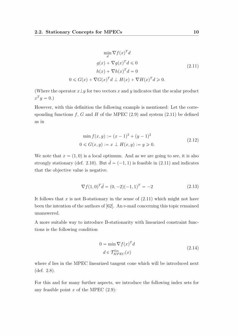
mind∇fpxqTd
gpxq `∇gpxqTd ď 0
hpxq `∇hpxqTd “ 0
0 ď Gpxq `∇GpxqTd K Hpxq `∇HpxqTd ě 0.
(2.11)
(Where the operator xKy for two vectors x and y indicates that the scalar product
xTy “ 0.)
However, with this definition the following example is mentioned: Let the corre-
sponding functions f , G and H of the MPEC (2.9) and system (2.11) be defined
as in
min fpx, yq :“ px´ 1q2 ` py ´ 1q2
0 ď Gpx, yq :“ x K Hpx, yq :“ y ě 0.(2.12)
We note that x “ p1, 0q is a local optimum. And as we are going to see, it is also
strongly stationary (def. 2.10). But d “ p´1, 1q is feasible in (2.11) and indicates
that the objective value is negative.
∇fp1, 0qT d “ p0,´2qp´1, 1qT “ ´2 (2.13)
It follows that x is not B-stationary in the sense of (2.11) which might not have
been the intention of the authors of [62]. An e-mail concerning this topic remained
unanswered.
A more suitable way to introduce B-stationarity with linearized constraint func-
tions is the following condition
0 “ min∇fpxqTdd P T linMPECpxq
(2.14)
where d lies in the MPEC linearized tangent cone which will be introduced next
(def. 2.8).
For this and for many further aspects, we introduce the following index sets for
any feasible point x of the MPEC (2.9):

2.2. Stationary Concepts for MPECs 11
Ig :“ ti | gipxq “ 0, i P t1, . . . , kuu
I`0 :“ ti | Gipxq ą 0, Hipxq “ 0, i P t1, . . . ,muu
I0` :“ ti | Gipxq “ 0, Hipxq ą 0, i P t1, . . . ,muu
I00 :“ ti | Gipxq “ 0, Hipxq “ 0, i P t1, . . . ,muu.
(2.15)
The definitions depend on the specific point x and are defined in this sense if no
further argument is present. Now we introduce the MPEC version of the Abadie-
CQ with a definition of the linearized tangent cone specialized for MPECs.
2.8 Definition (MPEC Abadie-CQ, [74] def. 3.1) Let x be a feasible point
for the MPEC (2.9). The MPEC-Abadie-CQ is satisfied at x if
T pxq “ T linMPECpxq (2.16)
whereT linMPEC :“ td P Rn such that:
∇gipxqTd ď 0, @i P Ig
∇hipxqTd “ 0, i “ 1, . . . , l
∇GipxqTd “ 0, @i P I0`
∇HipxqTd “ 0, @i P I`0
∇GipxqTd ě 0, @i P I00
∇HipxqTd ě 0, @i P I00
p∇GipxqTdqp∇Hipxq
Tdq “ 0, @i P I00u.
(2.17)
Remark 2.3
• The definition of B-stationarity (def. 2.7) is equivalent to the alternative
definition of (2.14) if we assume that the MPEC-Abadie-CQ holds.
• It always holds that T pxq Ď T linMPECpxq [74].
• The difference between the MPEC linearized tangent cone T linMPEC and the
general linearized tangent cone T lin at a point x of the MPEC (2.9) is the
last block of constraints
p∇GipxqTdqp∇Hipxq
Tdq “ 0, @i P I00. (2.18)
2.2. Stationary Concepts for MPECs 12
Thus the MPEC version of the linearized tangent cone is more restrictive
than the general version.
Working with the tangent cone is often impractical. Other stationary concepts
use formulations with dual multipliers in the same fashion as the KKT-conditions.
The following definitions are closely related to each other. It is, as Leyffer and
Munson wrote in [49], “the alphabet soup of MPEC stationarity”.
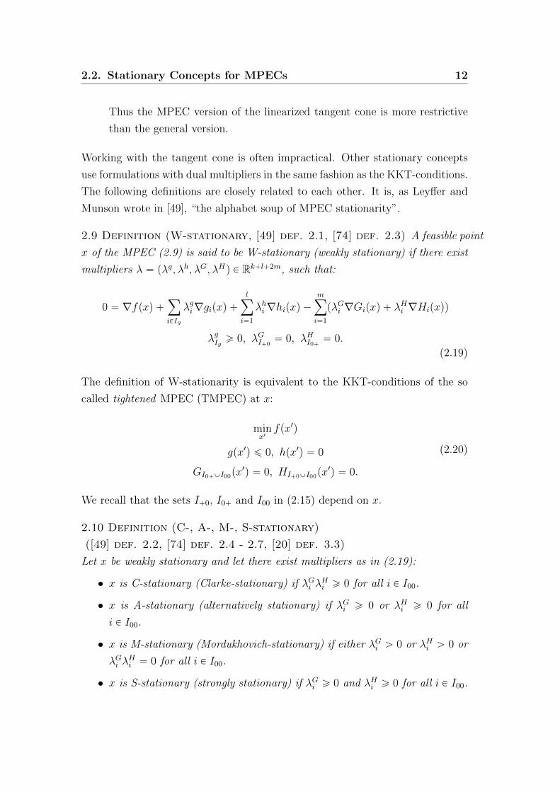
2.9 Definition (W-stationary, [49] def. 2.1, [74] def. 2.3) A feasible point
x of the MPEC (2.9) is said to be W-stationary (weakly stationary) if there exist
multipliers λ “ pλg, λh, λG, λHq P Rk`l`2m, such that:
0 “ ∇fpxq `ÿ
iPIg
λgi∇gipxq `lÿ
i“1
λhi∇hipxq ´mÿ
i“1
pλGi ∇Gipxq ` λHi ∇Hipxqq
λgIg ě 0, λGI`0“ 0, λHI0` “ 0.
(2.19)
The definition of W-stationarity is equivalent to the KKT-conditions of the so
called tightened MPEC (TMPEC) at x:
minx1
fpx1q
gpx1q ď 0, hpx1q “ 0
GI0`YI00px1q “ 0, HI`0YI00px
1q “ 0.
(2.20)
We recall that the sets I`0, I0` and I00 in (2.15) depend on x.
2.10 Definition (C-, A-, M-, S-stationary)
([49] def. 2.2, [74] def. 2.4 - 2.7, [20] def. 3.3)
Let x be weakly stationary and let there exist multipliers as in (2.19):
• x is C-stationary (Clarke-stationary) if λGi λHi ě 0 for all i P I00.
• x is A-stationary (alternatively stationary) if λGi ě 0 or λHi ě 0 for all
i P I00.
• x is M-stationary (Mordukhovich-stationary) if either λGi ą 0 or λHi ą 0 or
λGi λHi “ 0 for all i P I00.
• x is S-stationary (strongly stationary) if λGi ě 0 and λHi ě 0 for all i P I00.

2.2. Stationary Concepts for MPECs 13
The stationary concepts satisfy the following chains of inclusion [74, 49]:
pS ´ Stationaryq
ó
pM ´ Stationaryq
ó ó
pA´ Stationaryq pC ´ Stationaryq
ó ó
pW ´ Stationaryq
(2.21)
Example 2.1 The different concepts of stationarity are illustrated on an MPEC
with a single constraint for two non-negative complementary variables.
minw,ζPR
fpw, ζq
w, ζ ě 0
wζ “ 0
(2.22)
The index sets at p0, 0q are
I`0 “ I0` “ H, I00 “ t1u. (2.23)
Figure 2.1 illustrates the possible directions of the negative gradient ´∇fp0, 0qthat correspond to the individual MPEC stationary concepts. This means that if
the negative gradient lies in the indicated set of directions (blue) then the corre-
sponding stationary definition is satisfied at p0, 0q.
2.4 Theorem
Let x be a feasible point of the MPEC (2.9) and assume that the MPEC-Abadie-
CQ is satisfied at x.
1. If x is strongly stationary then x is B-stationary [74].
2. If f , g, h, G and H are continuously differentiable and x is locally optimal
then x is M-stationary [74].
3. A B-stationary point is not necessarily strongly stationary.

2.2. Stationary Concepts for MPECs 14
�
�
�
�
�
�
�
�
� − �������� − �������� � − �������� � − ��������
�
� − ��������
�
−∇� 0,0
Figure 2.1.: MPEC Stationary Concepts (Example 2.1)
Proof 1) Since the MPEC-Abadie-CQ is satisfied at x, we can use (2.14) to
characterize B-stationarity: d “ 0 solves
min∇fpxqTdd P T linMPECpxq.
(2.24)
By the definition of a strongly stationary point (def. 2.10) it follows that there
exist multipliers λ as in (2.19) with λGi ě 0 and λHi ě 0 for all i P I00. With
d P T linMPEC the following three cases may appear:
1. If i P I`0 it follows that ∇HipxqTd “ 0 and from (2.19) λGi “ 0.
2. If i P I0` it follows that ∇GipxqTd “ 0 and from (2.19) λHi “ 0.
3. If i P I00 it follows that ∇GipxqTd ě 0 and ∇Hipxq
Td ě 0 and from strong
stationarity that λGi , λHi ě 0.
Thus for any element d P T linMPECpxq it follows that
´∇fpxqTd “ pÿ
iPIg
λgi∇gipxq `lÿ
i“1
λhi∇hipxq ´mÿ
i“1
pλGi ∇Gipxq ` λHi Hipxqqq
Td
“ÿ
iPIg
λgiloomoon
ě0
∇gipxqTdloooomoooon
ď0
`
lÿ
i“1
λhi ∇hipxqTdloooomoooon
“0
´ÿ
iPI`0
p λGiloomoon
“0
∇GipxqTd` λHi ∇Hipxq
Tdloooomoooon
“0
q
´ÿ
iPI0`
pλGi ∇GipxqTd
loooomoooon
“0
` λHiloomoon
“0
∇HipxqTdq
´ÿ
iPI00
p λGiloomoon
ě0
∇GipxqTd
loooomoooon
ě0
` λHiloomoon
ě0
∇HipxqTd
loooomoooon
ě0
q ď 0.
(2.25)

2.2. Stationary Concepts for MPECs 15
This shows that x is B-stationary.
2) The proof for this point is not presented in detail here. For more information
the reader is referred to the related article [74] instead. The following is a brief
outline: First it can be shown that for affine linear functions g, h, G andH it holds
that any local solution x is M-stationary. In order to show this, the existence of
Fritz-John type multipliers is utilized. These always exist if the functions of an
optimization problem are continuously differentiable [74, thm. 2.1]. For further
information on Fritz-John multipliers see [22] section 2.2.5. Since the MPEC-
Abadie-CQ is satisfied, the case of affine linear constraint functions is sufficient.
The complete proof can be found in [74] theorem 3.1.
3) The following example shows a B-stationary point that is not strongly sta-
tionary:
minw,ζPR
´w ´ ζ
wζ “ 0
w, ζ ě 0
pζ ´ wqpζ ` wq “ 0
ζ ´ w ě 0
ζ ` w ě 0
(2.26)
The only feasible point of this system is p0, 0q which is obviously B-stationary.
Regarding the strong stationary condition, this would require positive multipliers
λ “ pλ1, λ2, λ3, λ4q ě 0 such that
0 “
˜
´1
´1
¸
´ λ1
˜
1
0
¸
´ λ2
˜
0
1
¸
´ λ3
˜
´1
1
¸
´ λ4
˜
1
1
¸
. (2.27)
The second of both components reveals that this equation cannot be satisfied for
λ ě 0 and thus p0, 0q is not strongly stationary. �
From point 3 of theorem 2.4 we see that the strong stationary condition is more
restrictive than what is needed for local optimality. On the other hand all the
weaker stationary concepts (W-, A-, C- and M-stationary) allow first order de-
scent directions. This can be seen with the following example [49, 2.7]:
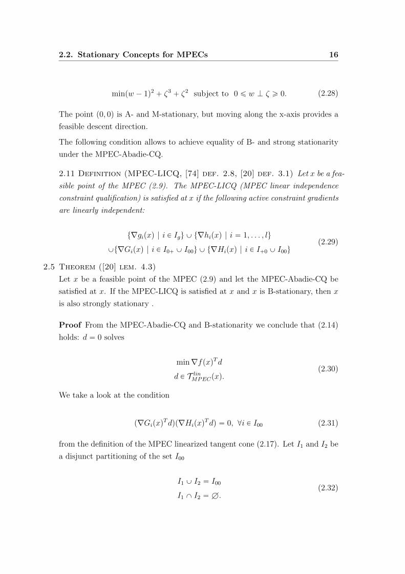
2.2. Stationary Concepts for MPECs 16
minpw ´ 1q2 ` ζ3` ζ2 subject to 0 ď w K ζ ě 0. (2.28)
The point p0, 0q is A- and M-stationary, but moving along the x-axis provides a
feasible descent direction.
The following condition allows to achieve equality of B- and strong stationarity
under the MPEC-Abadie-CQ.
2.11 Definition (MPEC-LICQ, [74] def. 2.8, [20] def. 3.1) Let x be a fea-
sible point of the MPEC (2.9). The MPEC-LICQ (MPEC linear independence
constraint qualification) is satisfied at x if the following active constraint gradients
are linearly independent:
t∇gipxq | i P Igu Y t∇hipxq | i “ 1, . . . , lu
Yt∇Gipxq | i P I0` Y I00u Y t∇Hipxq | i P I`0 Y I00u(2.29)
2.5 Theorem ([20] lem. 4.3)
Let x be a feasible point of the MPEC (2.9) and let the MPEC-Abadie-CQ be
satisfied at x. If the MPEC-LICQ is satisfied at x and x is B-stationary, then x
is also strongly stationary .
Proof From the MPEC-Abadie-CQ and B-stationarity we conclude that (2.14)
holds: d “ 0 solves
min∇fpxqTdd P T linMPECpxq.
(2.30)
We take a look at the condition
p∇GipxqTdqp∇Hipxq
Tdq “ 0, @i P I00 (2.31)
from the definition of the MPEC linearized tangent cone (2.17). Let I1 and I2 be
a disjunct partitioning of the set I00
I1 Y I2 “ I00
I1 X I2 “ H.(2.32)

2.2. Stationary Concepts for MPECs 17
Let T pI1, I2q Ď T linMPECpxq be the subset of the MPEC linearized tangent cone
where the constraint (2.31) is exchanged for a number of more restrictive linear
constraints:
T pI1, I2q :“ td P Rn such that:
∇gipxqTd ď 0, @i P Ig
∇hipxqTd “ 0, i “ 1, . . . , l
∇GipxqTd “ 0, @i P I0`
∇HipxqTd “ 0, @i P I`0
∇GipxqTd ě 0, @i P I00zI1
∇HipxqTd ě 0, @i P I00zI2
∇GipxqTd “ 0, @i P I1
∇HipxqTd “ 0, @i P I2u.
(2.33)
It follows that for each such partitioning pI1, I2q the vector d “ 0 is always an
optimal solution of the problem
min∇fpxqTdd P T pI1, I2q.
(2.34)
This is due to the fact that d “ 0 is always feasible and by the B-stationary
condition no solution with lower objective value can exist.
We notice that problem (2.34) is a pure LP, thus we can conclude that the KKT-
conditions are satisfied at d “ 0 and the following multipliers λ exist
0 “ ∇fpxq `ÿ
iPIg
λgi∇gipxq `lÿ
i“1
λhi∇hipxq ´mÿ
i“1
pλGi ∇Gipxq ` λHi ∇Hipxqq
λgIg ě 0
(2.35)
but with the following restrictions, depending on pI1, I2q
• for i P I2 there are active inequality constraints ∇GipxqTd ě 0 in the
definition of T pI1, I2q. It follows that λGI2 ě 0;
2.2. Stationary Concepts for MPECs 18
• for i P I1 there are active inequality constraints ∇HipxqTd ě 0 in the
definition of T pI1, I2q. It follows that λHI1 ě 0;
• for i P I`0 there are no constraints present for ∇GipxqTd in T pI1, I2q thus
it follows that λGI`0“ 0;
• for i P I0` there are no constraints present for ∇HipxqTd in T pI1, I2q thus
it follows that λHI0` “ 0.
With the MPEC-LICQ it follows that the multipliers of (2.35) are unique. Thus
for any partitioning pI1, I2q we will receive the same multipliers.
Since λGI2 ě 0 and λHI1 ě 0 for each partitioning it follows that λG, λH ě 0, @i P I00.
This concludes that the multipliers λ satisfy the requirements of definition 2.10
which shows that x is strongly stationary. �
Similar to the MPEC-LICQ there also exists an MPEC-MFCQ.
2.12 Definition (MPEC-MFCQ, [62] Def. 2.5) The MPEC-MFCQ is sat-
isfied at a feasible point x of the MPEC (2.9) if there exists a non-zero vector
d P Rn such that
∇GipxqTd “ 0, @i P I0`
∇HipxqTd “ 0, @i P I`0
∇hipxqTd “ 0, i “ 1, . . . , l
∇gipxqTd ą 0, @i P Ig
∇GipxqTd ą 0, @i P I00
∇HipxqTd ą 0, @i P I00
(2.36)
and the vectors of the following set are linearly independent
t∇Gipxq | i P I0`u Y t∇Hipxq | i P I`0u Y t∇hipxq | i “ 1, . . . , lu. (2.37)
We want to provide an example that explains why solving MPECs poses potential
difficulties. First we note that the standard MFCQ (def. 2.5) does not hold at
any point of the MPEC, since the gradients of the constraints

2.2. Stationary Concepts for MPECs 19
Gipxq ě 0, Hipxq ě 0, GipxqHipxq ď 0, @i “ 1, . . . ,m (2.38)
at a feasible point x are always linearly dependent with some positive multipliers.
But for various applications the MFCQ provides existence of KKT multipliers,
since it implies the Abadie-CQ. This is crucial for many non-linear solution meth-
ods.
The end of this section presents a helpful result which yields that an M-stationary
point is locally optimal under certain conditions without requiring the MPEC-
Abadie-CQ. For this we need two weaker forms of convexity:
2.13 Definition (Pseudo- and Quasiconvex, [52])
A differentiable function f : X Ñ R is called pseudoconvex if for x, y P X
∇fpxqpy ´ xq ě 0 ñ fpyq ě fpxq. (2.39)
A differentiable function f is called quasiconvex if
fpλx` p1´ λqyq ď maxtfpxq, fpyqu, @x, y P X. (2.40)
2.6 Theorem (Sufficient M-stationary condition, [74] Thm. 2.3)
Let x be an M-stationary point of the MPEC (2.9), i.e. there exist multipliers
such that
0 “ ∇fpxq `ÿ
iPIg
λgi∇gipxq `lÿ
i“1
λhi∇hipxq ´mÿ
i“1
pλGi ∇Gipxq ` λHi ∇Hipxqq
λgIg ě 0, λGI`0“ 0, λHI0` “ 0
either λGi ą 0, λHi ą 0 or λGi λHi “ 0, @i P I00.
(2.41)

2.2. Stationary Concepts for MPECs 20
Let the following index sets be defined as
J` :“ ti | λhi ą 0u, J´ :“ ti | λhi ă 0u,
I`00 :“ ti P I00 | λGi ą 0, λHi ą 0u,
I`00G :“ ti P I00 | λGi “ 0, λHi ą 0u, I´00G :“ ti P I00 | λ
Gi “ 0, λHi ă 0u,
I`00H :“ ti P I00 | λGi ą 0, λHi “ 0u, I´00H :“ ti P I00 | λ
Gi ă 0, λHi “ 0u,
I`0` :“ ti P I0` | λGi ą 0u, I´0` :“ ti P I0` | λ
Gi ă 0u,
I``0 :“ ti P I`0 | λHi ą 0u, I´`0 :“ ti P I`0 | λ
Hi ă 0u.
(2.42)
Let f be pseudoconvex at x and the following functions be quasiconvex:
gi for i P Ig, hi for i P I`J , ´hi for i P J´, Gi for i P I´0` Y I´00H , ´Gi for
i P I`0` Y I`00H Y I
`00, Hi for i P I´`0 Y I
´00G, ´Hi for i P I``0 Y I
`00G Y I
`00.
1. If I´0`YI´`0YI
´00GYI
´00H “ H it follows that x is a globally optimal solution
of the MPEC.
2. If either I´00G Y I´00H “ H or for all feasible x1 in a sufficiently small set
around x it holds that
Gipx1q “ 0, Hipx
1q “ 0, @i P I´00G Y I
´00H (2.43)
then x is a locally optimal solution of the MPEC.
The proof of this theorem can be found in [74], theorem 2.3.
With this result it is easy to derive optimality criteria for the case where the
constraint functions are affine linear and the objective function is convex. This
class of MPECs will be investigated in detail in the subsequent chapters.
Corollary 2.1
Let x be a feasible point of MPEC (2.9) and assume that f is convex and g, h,
G and H are affine linear.
1. If x is strongly stationary then x is locally optimal.
2. If x is strongly stationary and λGI0` ě 0 and λHI`0ě 0 then x is globally
optimal.

2.3. Solution Algorithms for MPECs 21
Proof 1) From strong stationarity follows M-stationarity and I´00G “ I´00H “ H.
The result follows with point 2 of theorem 2.6.
2) It further holds that
I´0` “ H ô λGI0` ě 0 (2.44)
I´`0 “ H ô λHI`0ě 0. (2.45)
And since x is strongly stationary it follows that
I´00G Y I´00H “ H. (2.46)
The result follows with point 1 of theorem 2.6. �
2.3. Solution Algorithms for MPECs
This section provides a small number of selected references to solution methods
and related articles for MPECs. Among them are algorithms, such as interior
point methods or regularization schemes, that will not be discussed in detail
within the extent of this work. The references are mainly in chronological order,
ending with three monographs that have a summarizing character.
In [51] Luo et al. present applications of PSQP (piece wise sequential quadratic
programming) methods to MPECs. Their results include local convergence under
the MPEC-LICQ.
In [64] Scholtes investigates a regularization scheme for MPECs as (2.9). The
regularization is based on:
min fpxq
gpxq ď 0, hpxq “ 0
Gpxq ě 0, Hpxq ě 0, GpxqiHpxqi ď t, i “ 1, . . . ,m
(2.47)
for a non-negative scalar t. He shows that under suitable assumptions a series
of stationary points of systems (2.47) converges to a C-stationary point of the
MPEC. The monograph [62] by Ralph and Wright establishes more properties
on algorithms with this regularization scheme. Another regularization scheme is
the Lin-Fukushima approach, as referenced below.

2.3. Solution Algorithms for MPECs 22
In [75] Zhang et al. present an algorithm that solves MPECs with convex ob-
jective function and affine linear complementarity constraints. The algorithm
investigates extreme points and directions around the current point of iteration.
These extreme elements determine a face of the feasible area around this cur-
rent point. The SQP step is then carried out on this face. At termination the
algorithm yields a locally optimal point.
In the monograph [60], Demiguel et al. present an interior point method for
relaxations of the following type.
The MPEC in [60] is defined as
minxfpxq
hpxq “ 0
0 ď Gpxq K Hpxq ě 0.
(2.48)
The relaxation for pδ1, δ2, δ3q ě 0 is
minpx,w,ζ,sq
fpxq
hpxq “ 0
Gpxq ´ w “ 0
Hpxq ´ ζ “ 0
s1 ´ w “ δ1
s2 ´ ζ “ δ2
s3 ` wT ζ “ δ3
w, ζ, s ě 0.
(2.49)
where the parameters δ1, δ2 and δ3 gradually decrease in their algorithm. The
vector s allows the possibility to rewrite the system with equality constraints.
Their article also holds a useful collection of references in the introduction.
In [25] Hu and Ralph investigate the application of penalty methods to MPECs.
In the monograph [20], Fletcher et al. investigate the local convergence of SQP
methods. Their article is helpful in understanding the difficulties with linear de-
pendent active constraints in MPEC solution methods. They achieve superlinear
convergence around a strongly stationary point under a number of reasonable
assumptions.
The monograph [49], by Leyffer and Munson, presents a globally convergent filter
method. In an iteration cycle, a linear problem is used to estimate the active
constraint set of the solution, then a QP with equality constraints is solved. By
applying a filter they achieve convergence to a B-stationary point of the MPEC.

2.4. Outlook 23
In [2] Audet et al. investigate reformulations of linear 0-1 mixed integer program-
ming problems to MPECs with linear objective function and linear complemen-
tarity constraints. They present the equivalent versions of cuts, such as e.g. the
common Gomory cuts from mixed integer programming, as well as branch-and-
cut strategies in the MPEC world. In relation to this, the monograph [55], by
Mitchell et al., focuses on tighter relaxations of MPECs.
In the monograph [37], Kanzow et al. show that the Lin-Fukushima-regularization
can create a series of NLPs whose stationary points converge to a C-stationary
point of the MPEC (2.9). For this, the complementarity constraints are replaced
by
pGipxq ` tqpHipxq ` tq ´ t2ě 0, i “ 1, . . .m
GipxqHipxq ´ t2ď 0, i “ 1, . . . ,m
(2.50)
for a non-negative scalar t that decreases during the algorithm.
In [30], Judice gives an overview of algorithms for MPECs with linear objective
function and linear complementarity constraints. An extensive bibliography on
bilevel programming and MPECs can be found in [68] by Dempe. The monograph
[31] by Judice contains a collection of solution techniques for MPECs with linear
complementarity constraints.
2.4. Outlook
The following chapter changes from the theoretical background of MPECs to a
practical quadratic problem that has its origin in an application related to the
automotive industry. After an introduction to the problem and some further
investigations on the matter of the solution map of quadric problems, the topic
of MPECs returns in section 3.4. In this section a bilevel problem is introduced
that can be formulated with the element of linear equilibrium constraints.

3. The Reweighting Problem
The automotive industry provides a good example of so called high complexity
products [50, 38, 67]. In this chapter a problem with complementarity con-
straints, which originates from a demand forecast model for multivariant product
configurations, is presented.
“Mass customization has been viewed as desirable but difficult to achieve
in the volume automotive sector.”
– Production and Operations Management [9]
Visiting the online configurator of a leading automotive manufacturer in the
premium segment provides a good impression on the topic [72]. The customer’s
choice depends not only on the specific model series, color and engine but is
extended to a large number of optional equipment ranging from interior design
to advanced driving assistance systems.
A complete customer order of a Mercedes-Benz R© vehicle holds the information
of a binary vector with hundreds of entries. It is considered highly likely that the
daily output of a single factory does not contain two identical vehicles.
Beyond what the customer can see lies a large rule-based documentation. This
translates the customer configuration into the technical information that is needed
to produce the vehicle in full detail (see [38] for additional information). The
documentation especially holds the list of all structural elements. Figure 3.1
shows a sample of the data format. Each row represents a technical part in
combination with its physical position that might possibly be present in the final
product. Whether or not it is present depends on the evaluation of a potentially
lengthy Boolean expression (column “Rule” in table 3.1). The variables of this
expression are (without further detail) the binary specifications of the customer
order. The fully translated vehicle holds the information of a binary vector with
about 10,000 entries, or a floating point vector with thousands of entries, if the
24

3.1. The Reweighting Problem 25
Technical Part Position Description Rule
A188780201 100-100.1Distance Ring
Park Distance Control189;
A188733208 120-120.1Pipe Cover
Brushed
(686^588) ^ (123 ^ 543^ 555
^ 678 _ 546) ^ (686 ^ 588);
A178669405 120-120.2Pipe Cover
Black(123 ^ 543 ^
555 ^ 678 _ 546) ^ (686 ^ 588);
A199725507 250-250.15
Combined Instrument:Odometer,
Oil-Pressure Control,White Backlight
(R272 ^ 766 ^ 434_ 344 ^ 665 ^ 455 _ 915)
^ (566 ^ 777)^ (458 _ 669 _ 155)^ (532 _ 343)^546 _ R32;
Table 3.1.: Format Sample of the Technical Documentation
demands for technical parts of the same type are accumulated. These entries are
denoted shortly as parts.
The increasing variety presents a challenge in acquiring detailed demand forecasts.
Considering the data of optional equipment selection in the layer of information
that is visible to the customer, we see that this layer holds aspects which are
observable for marketing and sales. However, extending the analysis and predic-
tion of customer and market behavior to the layer of parts and their demand is
difficult.
In the following section we present a given demand forecast model that is applica-
ble to any high complexity product. The model is based on a convex optimization
problem with a multicriterial objective function, and depends on a set of param-
eters which are related to a certain prognosis input: We assume that a sales or
marketing department (or some other source) provides a certain prognosis for
some of the optional equipment specifications in a future demand period. The
model connects this option planning input with the knowledge about historical
product configurations that hold information of customer behavior and previous
part demands.
The final step is to train this model with data scenarios that simulate the situ-
ation of a demand forecast requirement. The result of the forecast can then be
compared to the desired demand outcome and thus be evaluated. This, let us call
3.2. The Demand Forecast Model 26
it training phase, is conducted by solving a bilevel problem. The bilevel problem
can then be formulated as an MPEC and is subject to the solution techniques
that will be developed within the scope of this work.
3.2. The Demand Forecast Model
The demand forecast model is constructed in three steps. It is based on a param-
eter dependent convex optimization problem, and we focus on the aspects related
to its application.
1) Historical Data and a Vector based Representation
We assume that a set of product configurations exists that are suitable as a
foundation for the current demand forecast scenario. These might e.g. be con-
figurations of the same model series, or configurations that have been ordered in
the same market segment as the one that is currently of interest. Let us assume
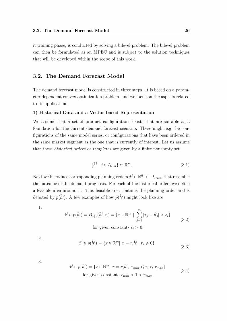
that these historical orders or templates are given by a finite nonempty set
thi | i P IHistu Ă Rm. (3.1)
Next we introduce corresponding planning orders xi P Rn, i P IHist, that resemble
the outcome of the demand prognosis. For each of the historical orders we define
a feasible area around it. This feasible area contains the planning order and is
denoted by pphiq. A few examples of how pphiq might look like are
1.
xi P pphiq “ B}¨}1phi, εiq “ tx P Rm
|
mÿ
j“1
|xj ´ hij| ă εiu
for given constants εi ą 0;
(3.2)
2.xi P pphiq “ tx P Rm
| x “ rihi, ri ě 0u;
(3.3)
3.xi P pphiq “ tx P Rm
| x “ rihi, rmin ď ri ď rmaxu
for given constants rmin ă 1 ă rmax.(3.4)
3.2. The Demand Forecast Model 27
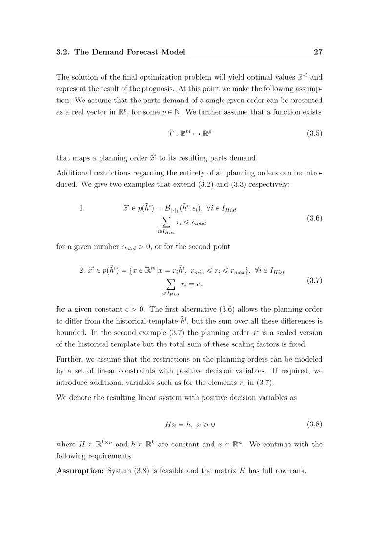
The solution of the final optimization problem will yield optimal values x˚i and
represent the result of the prognosis. At this point we make the following assump-
tion: We assume that the parts demand of a single given order can be presented
as a real vector in Rp, for some p P N. We further assume that a function exists
T : RmÞÑ Rp (3.5)
that maps a planning order xi to its resulting parts demand.
Additional restrictions regarding the entirety of all planning orders can be intro-
duced. We give two examples that extend (3.2) and (3.3) respectively:
1. xi P pphiq “ B}¨}1phi, εiq, @i P IHist
ÿ
iPIHist
εi ď εtotal(3.6)
for a given number εtotal ą 0, or for the second point
2. xi P pphiq “ tx P Rm|x “ rih
i, rmin ď ri ď rmaxu, @i P IHistÿ
iPIHist
ri “ c. (3.7)
for a given constant c ą 0. The first alternative (3.6) allows the planning order
to differ from the historical template hi, but the sum over all these differences is
bounded. In the second example (3.7) the planning order xi is a scaled version
of the historical template but the total sum of these scaling factors is fixed.
Further, we assume that the restrictions on the planning orders can be modeled
by a set of linear constraints with positive decision variables. If required, we
introduce additional variables such as for the elements ri in (3.7).
We denote the resulting linear system with positive decision variables as
Hx “ h, x ě 0 (3.8)
where H P Rkˆn and h P Rk are constant and x P Rn. We continue with the
following requirements
Assumption: System (3.8) is feasible and the matrix H has full row rank.

3.2. The Demand Forecast Model 28
We see that the first step in the modeling process is highly flexible. Each of
the given alternatives can be translated to a certain meaning in terms of the
manufacturer. Which approach is most suitable for the given situation depends
on the specific data, as well as on the expectations of the user.
2) Deviation of Planning and History
One intention behind this modeling concept is to preserve the information that
is contained in the vectors hi, i P IHist since it represents customer behavior.
We introduce a term that penalizes the deviation of the planning order from the
historical template. This term is then added to the objective function of the
model. A suitable example would be
minxi: iPIHist
nÿ
j“1
pxij ´ hijq
2. (3.9)
If we reconsider example (3.7) then (3.9) is equivalent to
minxi: ıPIHist
ÿ
iPIHist
pri ´ 1q2. (3.10)
To this point we notice that the optimization of the model penalizes the deviation
from the historical templates, and the historical templates are feasible at the same
time. Thus the model, in the current state, should simply return the historical
templates x˚i “ hi as a result. We continue with the last step where the objective
function becomes multicriterial.
3) Option Planning Rates
In the last step we want the model to reflect the option planning input that
is given beforehand. The option planning input reflects changes in the market
segment (or current planning area) on the level of option take rates. We assume
that this input is presented by a real vector b “ pb1, . . . , bmq that correspond to
the entries in the vector representation of both the historical data hi and the
planning output xi, i P IHist.
A prognosticated rate of bj0 for the component with index j0, is met if
ř
iPIHistxij0
cardpIHistq“ bj0 (3.11)
3.2. The Demand Forecast Model 29
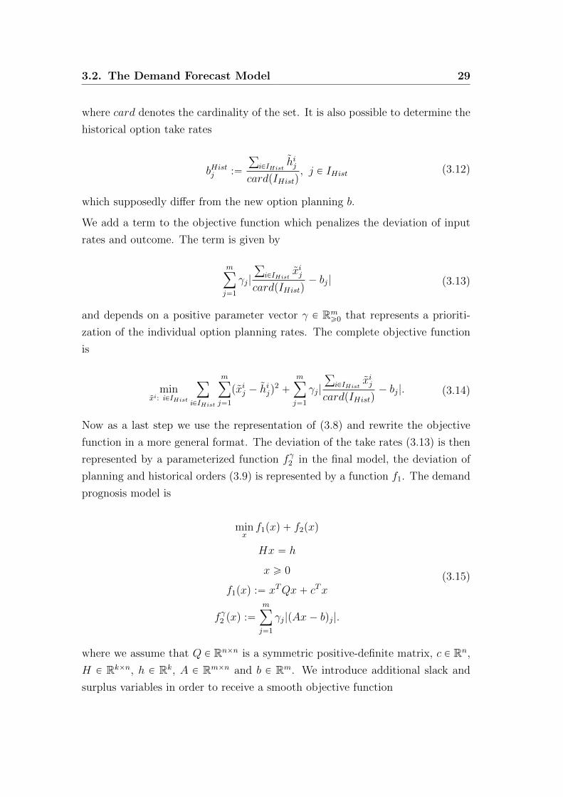
where card denotes the cardinality of the set. It is also possible to determine the
historical option take rates
bHistj :“
ř
iPIHisthij
cardpIHistq, j P IHist (3.12)
which supposedly differ from the new option planning b.
We add a term to the objective function which penalizes the deviation of input
rates and outcome. The term is given by
mÿ
j“1
γj|
ř
iPIHistxij
cardpIHistq´ bj| (3.13)
and depends on a positive parameter vector γ P Rmě0 that represents a prioriti-
zation of the individual option planning rates. The complete objective function
is
minxi: iPIHist
ÿ
iPIHist
mÿ
j“1
pxij ´ hijq
2`
mÿ
j“1
γj|
ř
iPIHistxij
cardpIHistq´ bj|. (3.14)
Now as a last step we use the representation of (3.8) and rewrite the objective
function in a more general format. The deviation of the take rates (3.13) is then
represented by a parameterized function fγ2 in the final model, the deviation of
planning and historical orders (3.9) is represented by a function f1. The demand
prognosis model is
minxf1pxq ` f2pxq
Hx “ h
x ě 0
f1pxq :“ xTQx` cTx
fγ2 pxq :“mÿ
j“1
γj|pAx´ bqj|.
(3.15)
where we assume that Q P Rnˆn is a symmetric positive-definite matrix, c P Rn,
H P Rkˆn, h P Rk, A P Rmˆn and b P Rm. We introduce additional slack and
surplus variables in order to receive a smooth objective function

3.2. The Demand Forecast Model 30
minpx,u,vq
xTQx` cTx`mÿ
j“1
γjpuj ` vjq
Hx “ h
Ax` u´ v “ b
x, u, v ě 0.
(3.16)
3.1 Definition (Reweighting Problem) The problem given by (3.16) is de-
noted the reweighting problem.
The term reweighting is related to the special case of the modeling approach (3.7)
where every planning order is a reweighted version of the corresponding historical
template. (See example 3.1 below.)
We have assumed the existence of a function T that maps a planning order xi
to its parts demand in (3.5). We now assume that we can find an equivalent
function
T : RnÞÑ Rp (3.17)
that maps a given vector x (that represents all planning orders) to the aggregated
parts demand. This means for a solution x˚ of (3.16) it holds
T px˚q “ÿ
iPIHist
T px˚iq. (3.18)
The value T px˚q represents the final output of the demand forecast model.
Example 3.1 (Reweighting Problem) We demonstrate the idea behind the
reweighting problem. Let a set of historical configurations h1, . . . , hn, for n “ 6
and m “ 5, be given by the entries in table 3.2. The last column shows the given
option planning that defines the vector b in (3.16).
We use the exemplary approach of (3.4) with rmin “ 0.5 and rmax “ 2 to build
the model. We also introduce a normalizing constraint
nÿ
i“1
ri “ n. (3.19)
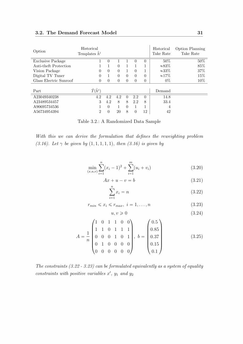
3.2. The Demand Forecast Model 31
OptionHistorical
Templates hiHistoricalTake Rate
Option PlanningTake Rate
Exclusive Package 1 0 1 1 0 0 50% 50%Anti-theft Protection 1 1 0 1 1 1 «83% 85%Vision Package 0 0 0 1 0 1 «33% 37%Digital TV Tuner 0 1 0 0 0 0 «17% 15%Glass Electric Sunroof 0 0 0 0 0 0 0% 10%
Part T phiq Demand
A23049340238 4.2 4.2 4.2 0 2.2 0 14.8A23489534457 3 4.2 8 8 2.2 8 33.4A90695734536 1 0 1 0 1 1 4A56734954394 2 0 20 8 0 12 42
Table 3.2.: A Randomized Data Sample
With this we can derive the formulation that defines the reweighting problem
(3.16). Let γ be given by p1, 1, 1, 1, 1q, then (3.16) is given by
minpx,u,vq
nÿ
i“1
pxi ´ 1q2 `mÿ
i“1
pui ` viq (3.20)
Ax` u´ v “ b (3.21)nÿ
i“1
xi “ n (3.22)
rmin ď xi ď rmax, i “ 1, . . . , n (3.23)
u, v ě 0 (3.24)
A “1
n
¨
˚
˚
˚
˚
˚
˚
˝
1 0 1 1 0 0
1 1 0 1 1 1
0 0 0 1 0 1
0 1 0 0 0 0
0 0 0 0 0 0
˛
‹
‹
‹
‹
‹
‹
‚
, b “
¨
˚
˚
˚
˚
˚
˚
˝
0.5
0.85
0.37
0.15
0.1
˛
‹
‹
‹
‹
‹
‹
‚
(3.25)
The constraints (3.22 - 3.23) can be formulated equivalently as a system of equality
constraints with positive variables x1, y1 and y2
3.2. The Demand Forecast Model 32
¨
˚
˝
eT 0 0
I ´I 0
I 0 I
˛
‹
‚
looooooomooooooon
“H
¨
˚
˝
x1
y1
y2
˛
‹
‚
“
¨
˚
˝
n
rmine
rmaxe
˛
‹
‚
loooomoooon
“h
x1, y1, y2 ě 0
(3.26)
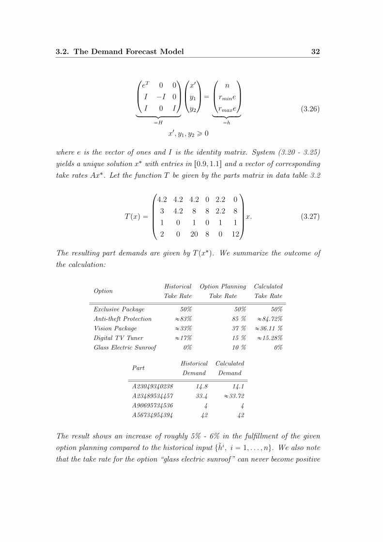
where e is the vector of ones and I is the identity matrix. System (3.20 - 3.25)
yields a unique solution x˚ with entries in r0.9, 1.1s and a vector of corresponding
take rates Ax˚. Let the function T be given by the parts matrix in data table 3.2
T pxq “
¨
˚
˚
˚
˚
˝
4.2 4.2 4.2 0 2.2 0
3 4.2 8 8 2.2 8
1 0 1 0 1 1
2 0 20 8 0 12
˛
‹
‹
‹
‹
‚
x. (3.27)
The resulting part demands are given by T px˚q. We summarize the outcome of
the calculation:
OptionHistorical
Take Rate
Option Planning
Take Rate
Calculated
Take Rate
Exclusive Package 50% 50% 50%
Anti-theft Protection «83% 85 % «84.72%
Vision Package «33% 37 % «36.11 %
Digital TV Tuner «17% 15 % «15.28%
Glass Electric Sunroof 0% 10 % 0%
PartHistorical
Demand
Calculated
Demand
A23049340238 14.8 14.1
A23489534457 33.4 «33.72
A90695734536 4 4
A56734954394 42 42
The result shows an increase of roughly 5% - 6% in the fulfillment of the given
option planning compared to the historical input thi, i “ 1, . . . , nu. We also note
that the take rate for the option “glass electric sunroof” can never become positive
3.2. The Demand Forecast Model 33
with this particular approach, since no historical template hi with this option is
present.
For the part demands we notice that some entries have not changed. However,
the first entry has changed by roughly 5% in comparison to its predecessor.
Real data instances have a large dimension n and can consider several thousand
units. A change of 5% in demand can be of interest in such scenarios.
3.1 Theorem
With the assumption that Hx “ h, x ě 0, is feasible and Q positive-definite, it
holds that for every vector γ ě 0 the reweighting problem (3.16) has a unique
finite solution px˚, u˚, v˚q.
Proof We look at the non-differentiable and the practical model of the reweight-
ing problem (3.15) and (3.16) respectively.
Problem (3.15):
minxf1pxq ` f2pxq
Hx “ h
x ě 0
f1pxq :“ xTQx` cTx
fγ2 pxq :“mÿ
j“1
γj|pAx´ bqj|.
Problem (3.16):
minpx,u,vq
xTQx` cTx`mÿ
j“1
γjpuj ` vjq
Hx “ h
Ax` u´ v “ b
x, u, v ě 0.
We notice that (3.15) is equivalent to (3.16) in the following sense:
The vector px˚, u˚, v˚q is a solution of (3.16) if and only if x˚ is a solution of
(3.15) and
u˚i “ maxt0, pb´ Ax˚qiu, i “ 1, . . . ,m
v˚i “ maxt0,´pb´ Ax˚qiu, i “ 1, . . . ,m.(3.28)
Next we show that a finite solution for both problems exists:
The objective function of (3.15) is convex since it is the sum of convex functions.
To see that fγ2 is convex we recall that γ ě 0. With Q positive-definite, it follows

3.3. Continuity of the Solution Map and Variational Inequalities 34
that f1 (and thus the objective function of (3.15)) is not only convex but strictly
convex.
From the quadratic term xTQx it also follows that (3.15) cannot be unbounded.
With the assumption that Hx “ h is feasible, it follows that (3.15) is feasible.
On a convex set it holds that a finite minimum of a strictly convex function
is unique, and thus it follows that the reweighting problem has a unique finite
solution. �
3.3. Continuity of the Solution Map and Variational
Inequalities
We want to investigate the parameter dependency of the reweighting problem
(3.16) on the parameter vector γ. The solution map of quadratic problems has
been widely investigated, and we gather some of the related results. The appli-
cation to a bilevel problem based on the reweighting problem is presented in the
following section.
For this section let a general quadratic problem be given by
minx
1
2xTQx` cTx
Ax ď b
Hx “ h
(3.29)
for a symmetric matrix Q P Rnˆn, c P Rn, A P Rmˆn, b P Rm, H P Rkˆn and
h P Rk.
3.2 Definition (Multifunction, [47] 7.2) Let F be a function that maps a
point in Rn to a set in Rm, for some n,m P N. Then we write F : Rn Ñ 2Rm
and F is denoted a multifunction.
3.3 Definition (Graph) Let F be a multifunction, the graph is defined by
graphF :“ tpx, yq P Rnˆ Rm
| y P Fpxqu. (3.30)

3.3. Continuity of the Solution Map and Variational Inequalities 35
3.4 Definition (Locally Upper Lipschitz Multifunction, [47] def. 7.4)
A multifunction F : Rn Ñ 2Rm is called locally upper Lipschitz at x if there exists
a constant l ą 0 and a neighborhood Ux of x such that
Fpxq Ď Fpxq ` l}x´ x}BRm , @x P Ux
Fpxq ` l}x´ x}BRm :“ ty1 ` y2 | y1 P Fpxq, }y2} ă l}x´ x}u.(3.31)
3.5 Definition (Upper Semicontinuous, [47] def. 8.2) A multifunction F :
Rn Ñ 2Rm is said to be upper semicontinuous at x if for any open neighborhood
V of Fpxq there exists a neighborhood U of x such that for all x in U it holds
that Fpxq is a subset of V .
3.1 Lemma
If the multifunction F is locally upper Lipschitz then it follows that F is upper
semicontinuous.
Further, if F is a multifunction that maps each point of Rn to a set in Rm with
exactly one element, then
• if F is locally upper Lipschitz, then it is locally Lipschitz continuous in the
sense of a single-valued function;
• if F is upper semicontinuous, then it is continuous in the sense of a single-
valued function.
Proof Assume that F is locally upper Lipschitz at x, and V an open neighbor-
hood of Fpxq. There exist Ux and l as in (3.31). We choose 0 ă l1 ă l such that
Bpx, l1q Ď V .
For every x P Ux where }x´ x} ă 1 it follows
Fpxq Ď Fpxq ` l}x´ x}BRm Ď Fpxq ` l1BRm Ď V. (3.32)
This shows that F is upper semicontinuous. The second part of the theorem
follows straight from (3.31) and the common ε-δ-definition of continuity respec-
tively.
3.6 Definition (Polyhedral Multifunction, [47] def. 7.3)
A multifunction F is denoted a polyhedral multifunction if its graph can be rep-
3.3. Continuity of the Solution Map and Variational Inequalities 36
resented by a finite union of convex polytopes in RnˆRm. Furthermore such sets
will also be denoted polyhedral.
We want to note the following important result.
3.2 Theorem ([47] Theorem 7.2)
If F : Rn Ñ 2Rm is a polyhedral multifunction, then there exists a fixed constant
l0 ą 0 such that F is locally Lipschitz in Rn with l “ l0 in (3.31). Then F is
called an upper Lipschitz multifunction.
Theorem 3.2 is intuitive if we think of F as the inverse projection of a union M
of polytopes in Rm`n to a linear subspace of dimension n. On a path in M , that
connects two point x and y in M , the change from Fpxq to Fpyq is determined by
the finitely many faces of the polytopes. From this finite number of affine linear
functions one can derive the desired constant l0. For a detailed proof the reader
is referred to the monograph [47] and the references therein.
The following lemma is an extended version of proposition 7.2 in [47]. For this
we note the KKT system of the QP (3.29):
Qx` c` ATλ´HTµ “ 0
Ax ď b
Hx “ h
λT pb´ Axq “ 0
λ ě 0.
(3.33)
Let Q, A and H be fixed. We define the following set X
XQP :“ tpc, h, x, λ, µq P R2n`2k`m| pc, h, x, λ, µq is feasible in (3.33)u. (3.34)
3.2 Lemma
Let π be the projection from R2n`2k`m to a linear subspace Rl. Let the multi-
function F : Rl Ñ R2n`2k`m be defined by
Fpyq “ π´1pyq XXQP . (3.35)
Then it holds that F is a polyhedral multifunction.

3.3. Continuity of the Solution Map and Variational Inequalities 37
Proof Without limitation of generality we assume that πpc, h, x, λ, µq “ c. The
graph of F is then given by
graphF “ tpc, c, h, x, λ, µq | pc, h, x, λ, µq P Xu. (3.36)
Thus it is sufficient to show that X is a finite union of polytopes.
Let s Ď t1, . . . ,mu be a subset. We define the set
Gpsq :“ X X tpb´ Axqi “ 0 @i P s, λi “ 0 @i R su. (3.37)
The definition of G is designed so that within this definition the complementarity
constraints in the definition of XQP (3.33) become redundant. It follows that Gpsq
is a polytope. We note that
X “ď
sĎt1,...,mu
Gpsq (3.38)
which yields that X is a finite union of polytopes and F is a polyhedral multi-
function. �
Lemma 3.2 is related to proposition 7.2 in [47] which characterizes the solution
set of a so called affine variational inequality problem (AVI) which can be stated
with the real matrices and vectors of the QP (3.29):
Find x P ∆ such that pQx` cqT py ´ xq ě 0, @y P ∆
∆ :“ ty | Ay ď b, Hy “ hu.(3.39)
We see that the term Qx ` c is the gradient of the objective function in (3.29).
Thus (3.39) provides a sufficient and necessary criterion for a local optimal point
x which can then be related to the KKT multipliers. In combination with lemma
3.2 or proposition 7.2 in [47] it follows that the solution map of every quadratic
problem is an upper Lipschitz multifunction.
The general version of a variational inequality is given by the following definition.
3.7 Definition (Variational Inequality, [42] 1.1) Let U be a nonempty,
closed and convex subset of the n-dimensional Euclidean space Rn, and G : U Ñ

3.4. The Reweighting Bilevel Problem 38
Rn continuous. The variational inequality problem is finding a point u˚ P U such
that
Gpu˚qT pu´ u˚q ě 0, @u P U. (3.40)
The monograph [48] provides an analysis of the continuity (upper and lower) of
the solution map of quadratic problems. A proof of the upper Lipschitz property
can also be found in [13] and a deeper analysis on linear perturbations of varia-
tional inequalities can be found in [47]. For a collection of various results on the
subject of variational inequalities see e.g. [42] or [40].
3.4. The Reweighting Bilevel Problem
We want to investigate the parameter dependency of the reweighting problem
(3.16) which has the following intention.
Say we have acquired a collection of historical data, including historical templates
and an option planning input. We further assume that we have defined the model
as in formulation (3.16) and established a function T , as in (3.17) and (3.20 -
3.25), that yields the respective part demand.
We further assume that there is a given part demand t that corresponds to the
desired outcome of the reweighting problem, i.e. we are in a training scenario
where the outcome of the reweighting problem is evaluated by calculating T pxq´t.
This is called an ex-post data scenario.
We formulate the reweighting bilevel problem for a given parameter set Γ, where Γ
is a polytope, and for an objective function that minimizes the length of T pxq´ t:
minγ}T px˚q ´ t}2
x˚ solves the reweighting problem p3.16q
γ P Γ.
(3.41)
We reformulate (3.41) with the KKT-conditions of the reweighting problem

3.4. The Reweighting Bilevel Problem 39
minpγ,x,u,v,λ,µ,sx,su,svq
}T pxq ´ t}2
Qx` c´HTµ´ ATλ´ sx “ 0
´λ` γ ´ su “ 0
λ` γ ´ sv “ 0
Ax` u´ v “ b
Hx “ h
0 ď psx, su, svq K px, u, vq ě 0
γ P Γ.
(3.42)
With theorem 2.1 and theorem 2.2 it follows that the KKT-conditions are nec-
essary and sufficient for every QP with positive semi-definite quadratic matrix.
This includes the reweighting problem (3.16) and implies that (3.41) and (3.42)
are equivalent.
We investigate the constraint system to determine that a number of decision
variables can be eliminated. Since Q is positive definite we can rewrite the first
entry in the constraint set to
x “ xpλ, µ, sxq :“ ´Q´1c`Q´1HTµ`Q´1ATλ`Q´1sx. (3.43)
We recall that H has full row rank by assumption. It follows that Hx “ h if and
only if
h “ ´HQ´1c`HQ´1HTµ`Q´1ATλ`Q´1sx
ô µ “ µpλ, sxq :“ pHQ´1HTq´1ph`HQ´1c´Q´1ATλ´Q´1sxq
and thus
x “ xpλ, sxq :“ xpλ, µpλ, sxq, sxq.
(3.44)
For the other constraints we can distinguish the following three cases. For any
feasible point in (3.42) it holds:
• If pb´ Axqi ą 0 then ui ą 0 which yields that su “ 0 which yields λi “ γi;
• If pb´ Axqi “ 0 then su, sv ě 0 which yields ´γi ď λi ď γi;

3.4. The Reweighting Bilevel Problem 40
• If pb´Axqi ă 0 then vi ą 0 which yields that sv “ 0 which yields λi “ ´γi.
In accordance to this, we introduce the following index sets
I` “ I`pxq “ ti | pb´ Axqi ą 0u Ď t1, . . . ,mu
I´ “ I´pxq “ ti | pb´ Axqi ă 0u Ď t1, . . . ,mu
I0 “ I0pxq “ ti | pb´ Axqi “ 0u Ď t1, . . . ,mu.
(3.45)
The feasible area of (3.42) can now be reformulated to obtain the following pre-
sentation:
minpγ,λ,sxq
}T pxpλ, sxqq ´ t}2
λi “ γi, @i P I`pxpλ, sxqq
´γi ď λi ď γi, @i P I0pxpλ, sxqq
λi “ ´γi, @i P I´pxpλ, sxqq
0 ď sx K xpλ, sxq ě 0
γ P Γ.
(3.46)
Let X denote the feasible area of (3.46)
X :“ tpγ, λ, sxq | pγ, λ, sxq feasible in (3.46)u. (3.47)
Let Fx : Γ Ñ 2Rn`2m
denote the solution map that assigns γ P Γ to the solutions
px˚, u˚, v˚q of the reweighting problem (3.16) i.e. px˚, u˚, v˚q P Fxpγq if and only
if px˚, u˚, v˚q is the solution of (3.16) for the given vector γ.
Similarly let Fpλ,sxq be the multifunction that finds the solutions of the KKT
system
Fpλ,sxqpγq :“ tpλ, sxq | pγ, λ, sxq P Xu. (3.48)
3.3 Theorem
Assume that Γ Ď Rmě0 is a polytope and that the matrices Q, A, H, h and b are
fixed.
1) It holds that for each γ P Γ: Fxpγq has exactly one element.

3.4. The Reweighting Bilevel Problem 41
Further, the function Fx : γ ÞÑ px, u, vq P Fxpγq is continuous in the sense of a
single valued function and the solution set FxpΓq of the reweighting problem is a
connected union of polytopes.
2) The multifunction Fpλ,sxq is upper Lipschitz and the feasible area of the
reweighting bilevel problem X is connected.
Proof 1) Theorem 3.1 determines that the reweighting problem has a unique
solution that exists.
Since the quadratic matrix Q in the reweighting bilevel problem is positive semi-
definite, it follows that the KKT-conditions are necessary and sufficient. Thus
lemma 3.2 yields that Fx is a polyhedral multifunction. With theorem 3.2 it
follows that Fx is upper Lipschitz. This implies that Fx is locally upper Lipschitz
and this implies that Fx is upper semicontinuous. Lemma 3.1 yields that Fx is
continuous in the sense of a single valued function which is equivalent to: Fx is
continuous.
Since Γ is a polytope by assumption and Fx is a polyhedral multifunction we
can conclude that FxpΓq is a union of polytopes and since FxpΓq is continuous it
follows that FxpΓq is connected as the image of a connected set under a continuous
function.
2) As in case 1 lemma 3.2 yields that Fpλ,sxq is a polyhedral multifunction. With
theorem 3.2 it follows that Fpλ,sxq is upper Lipschitz.
For two points pγ1, λ1, s1xq, pγ
2, λ2, s2xq P X we show that there exists a connecting
path in X. Let pγ be the connecting line between γ1 and γ2 in Γ. Since X is
finite union of polytopes Pi (lemma 3.2) it follows that we find a lifted version pi
of pγ in each of the polytopes Pi such that
pγ “ rγ1, γ2
srγ2, γ3srγ3, γ4
s ¨ ¨ ¨ Ď Γ
πγppiγq “ tγ | pγ, λ, sxq P p
iγu “ rγ
i, γi`1s.
(3.49)
The bracket notation in (3.49) denotes the concatenation of (a finite number of)
line segments.
Since Pi is a polytope, without limitation of generality, we can assume that the
lifted path pi is also a line segment. It remains to show that the end points
3.4. The Reweighting Bilevel Problem 42
of these lifted paths can be glued together by some other paths in order to re-
ceive a resulting path from pγ1, λ1, s1xq to pγ2, λ2, s2
xq in X which shows that X is
connected.
To see this we take a look at the subset of X for a fixed vector γ “ γ0. First we
note that Fxpγ0q has only a single element which has been shown in part 1 of the
proof. For Fpλ,sxqpγ0q it holds that there is only one possible value of x “ xpλ, sxq
(as defined in (3.43) and (3.44)). This means that the index sets I`, I´ and I0
in (3.46) are immutable in Fpλ,sxqpγ0q. It follows that Fpλ,sxqpγ0q is a polytope.
From this we can conclude that we can find a connecting line segment for the end
point of piγ and the start point of pi`1γ in X. With these additional line segments
we can glue the pieces piγ and receive a connecting path in X which shows that
X is connected. �
3.4.1. The Practical Reweighting Bilevel Problem
For the practical application with real data instances the parameter set is defined
as
Γ “ tγ | γmin ď γi ď γmax, i “ 1, . . . ,mu (3.50)
for two given constants γmax ą 1 ą γmin ą 0.
Additionally experiments have shown that, for the data at hand, the cases where
sx ‰ 0 are less interesting or non-desirable. Thus by assuming sx “ 0 we eliminate
the variables sx and achieve simplification in the practical version of the problem.
We also introduce a new matrix Aλ and vector bλ in order to rewrite the affine
linear function xpλ, sxq in the definition of the index sets I`, I´ and I0
Axpλ, 0q ´ b “ Aλλ´ bλ. (3.51)
The convex upper level objective function is defined by a matrix T :
T pxq “ T ¨ xpλ, sxq (3.52)

3.5. An Algorithmic Concept 43
and we minimize }Txpλ, sxq ´ t}2. Then immediately introduce another matrix
Tλ and vector tλ such that
Txpλ, 0q ´ t “ Tλλ´ tλ. (3.53)
With the information above the practical reweighting bilevel MPEC is defined by
minλ}Tλλ´ tλ}
2
λi ě γmin, if pbλ ´ Aλλqi ą 0 p: I`q
λi ď ´γmin, if pbλ ´ Aλλqi ă 0 p: I´q
´γmax ď λi ď γmax, i “ 1, . . .m.
(3.54)
3.8 Definition (Reweighting Bilevel Problem) The practical reweight-
ing bilevel problem or reweighting bilevel MPEC is problem (3.54) with the intro-
duction of additional slack and surplus variables and is given by
minpλ,w1,w2,ζ1,ζ2q
}Tλλ´ tλ}2
Aλλ` w1´ w2
“ bλ
λi ` ζ1i ě λmin, i “ 1, . . . ,m
λi ´ ζ1i ď ´λmin, i “ 1, . . . ,m
´λmax ď λi ď λmax, i “ 1, . . . ,m
0 ď pw1, w2q K pζ1, ζ2
q ě 0.
(3.55)
where Tλ P Rmˆp is a positive semi-definite matrix, Aλ P Rmˆm, tλ P Rp, bλ P Rm
and
λmax “ γmax ą 1 ą λmin “ γmin ą 0 (3.56)
are two constants.
3.5. An Algorithmic Concept
We have gained the knowledge that the feasible set of the practical reweighting
bilevel problem (3.55) is a connected union of polytopes (theorem 3.3). This

3.5. An Algorithmic Concept 44
inspires the following idea: We let I`, I´ and I0 be a partitioning of the set
t1, . . . ,mu corresponding to the constraints in (3.54). We solve the convex prob-
lem that is assumed to be feasible:
minλ}Tλλ´ tλ}
2
λi ě λmin, pbλ ´ Aλλqi ě 0, @i P I`
λi ď ´λmin, pbλ ´ Aλλqi ď 0, @i P I´
pb´ Aλλq “ 0, @i P I0
´λmax ď λi ď λmax, i “ 1, . . .m.
(3.57)
At the optimal point λ˚ we investigate the dual multipliers, and perform a step
in an active set strategy on the generally non-convex solution set. For a general
reference on active set strategies the reader is referred to [59].
Let ri be the dual multiplier of some constraint pbλ ´ Aλλqi „ 0, where the sign
of the equation depends on i P I` or i P I´ or i P I0, then
• if ri ă 0 and i P I` and λi “ λmin: move i to I0;
• if ri ă 0 and i P I´ and λi “ ´λmin: move i to I0;
• if ri ă 0 and i P I0 and λi ď ´λmin: move i to I´;
• if ri ă 0 and i P I0 and λi ě λmin: move i to I`.
Similarly for a multiplier rλi for one of the constraints λi ě λmin or λi ď ´λmin
we progress by the following changes:
• if rλi ă 0 and λi “ λmin and i P I` and pbλ ´ Aλλq “ 0: move i from I` to
I0;
• if rλi ă 0 and λi “ ´λmin and i P I´ and pbλ ´ Aλλq “ 0: move i from I´
to I0.
After one or more indices have been shifted, the next convex problem (3.57) is
solved. The algorithm will generate a series of points with descending objective
value. This is due to the fact that the solution of the previous convex problem is
still feasible for the convex problem of the next iteration. Since the feasible area
has shown to be connected (theorem 3.3), one may hope that the algorithm even
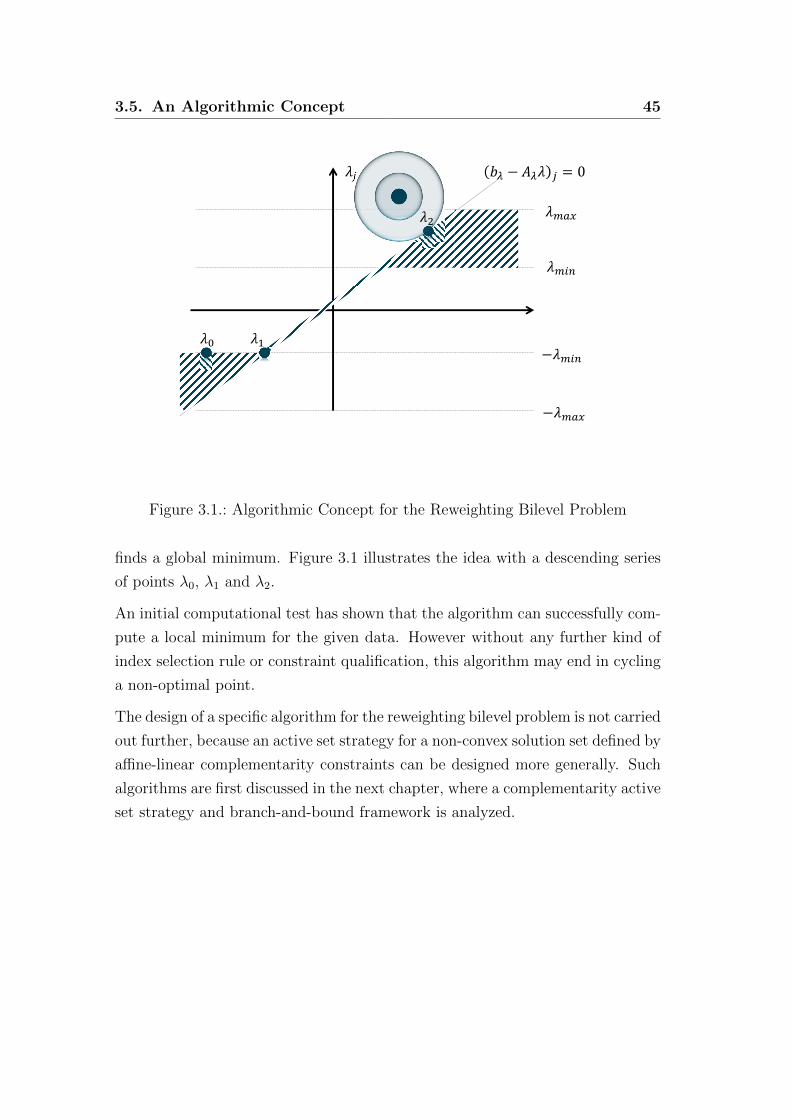
3.5. An Algorithmic Concept 45
Daimler AG Application of a Complementarity Active Set Strategy in Multi-Variant Product Demand Forecast / Maximilian Heß / 28.10.2016 Page 21
�� �� � ��� � � 0
��
��
���
���
�� ��
��
Figure 3.1.: Algorithmic Concept for the Reweighting Bilevel Problem
finds a global minimum. Figure 3.1 illustrates the idea with a descending series
of points λ0, λ1 and λ2.
An initial computational test has shown that the algorithm can successfully com-
pute a local minimum for the given data. However without any further kind of
index selection rule or constraint qualification, this algorithm may end in cycling
a non-optimal point.
The design of a specific algorithm for the reweighting bilevel problem is not carried
out further, because an active set strategy for a non-convex solution set defined by
affine-linear complementarity constraints can be designed more generally. Such
algorithms are first discussed in the next chapter, where a complementarity active
set strategy and branch-and-bound framework is analyzed.
4. CASET and BBASET
In section 3.5 we have seen the idea of an active set strategy that progresses over
a non-convex set defined by a union of polytopes. In [35] Judice et al. present
results for a complementarity active set algorithm for mathematical problems
with equilibrium constraints denoted as CASET.
4.1. CASET
Let the MPEC be defined by
minxfpxq
Cx “ Cyy ` Cww ` Cζζ “ g
y P Ky
x “ py, w, ζq ě 0
wT ζ “ 0
(4.1)
where Cy P Rkˆl, Cw P Rkˆm, Cζ P Rkˆm and C “ pCy, Cw, Cζq are real matrices,
g P Rk and f : Rn Ñ R continuously differentiable, n “ k ` 2m and Ky is a
polytope in Rl
Ky :“ ty | Ay “ bu (4.2)
where A P Rpˆl and b P Rp.
The idea is to run an active set strategy with two working sets Lw, Lζ Ď t1, . . . ,mu
that correspond to the constraints
wi “ 0, @i P Lw
ζi “ 0, @i P Lζ .(4.3)
46
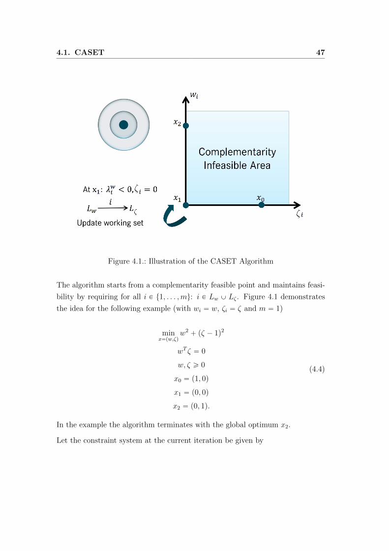
4.1. CASET 47
Figure 4.1.: Illustration of the CASET Algorithm
The algorithm starts from a complementarity feasible point and maintains feasi-
bility by requiring for all i P t1, . . . ,mu: i P Lw Y Lζ . Figure 4.1 demonstrates
the idea for the following example (with wi “ w, ζi “ ζ and m “ 1)
minx“pw,ζq
w2` pζ ´ 1q2
wT ζ “ 0
w, ζ ě 0
x0 “ p1, 0q
x1 “ p0, 0q
x2 “ p0, 1q.
(4.4)
In the example the algorithm terminates with the global optimum x2.
Let the constraint system at the current iteration be given by

4.1. CASET 48
Cyy ` Cww ` Cζζ “ g
Ay “ b
wi “ 0, @i P Lw p: λwi q
ζi “ 0, @i P Lζ p: λζi q
yi “ 0, @i P Ly Ď t1, . . . , ku p: λyi q.
(4.5)
where pλy, λw, λζq denote the dual multipliers. (These multipliers exist by theo-
rem 2.1.) System (4.5) is written as
Djx “ dj (4.6)
where j is the index of the current iteration. The convergence of the algorithm
depends on the following property:
Non-Degeneracy Assumption: The matrix Dj always has full row rank.
The CASET algorithm as in [35] is given by step 0 to 4 in algorithm 1 and 2.
Remark 4.1
1. If f is convex and the algorithm terminates with a strongly stationary
point in step 1, with corollary 2.1 it follows that a local optimal solution
was found.
2. The selection of the descent direction in step 2 and the selection of the step-
size in step 3 need additional conditions in order to ensure the convergence
to a stationary (i.e. KKT) point of (4.7). Line search methods have been
explored by many authors [10, 59, 5]. A convergence result for a direction
and stepsize rule is given in the following theorem 4.1.
3. Assume that KKT-points of (4.7) are detected in a finite number of steps. If
the non-degeneracy assumption was not present, then the algorithm could
potentially be caught in a cycle. This can be seen with the example of point
3 in theorem 2.4. The algorithm would then repeat switching the indices
of linearly dependent complementarity constraints between the sets Lw and

4.1. CASET 49
Step 0 (Initialization): Let xj denote the solution of the current iterationand initialize with a feasible point x0;Initialize Dj and hj with the active constraints at x0 as defined by (4.5);
Step 1 (Termination): If xj is not a KKT-point for the problem
min fpxq
Djx “ hj(4.7)
then go to step 2. Otherwise there exist multipliers µ such that
DTj µ “ ∇fpxjq (4.8)
and µ is unique by the non-degeneracy assumption. If
λyi ě 0, @i P Ly
λwi ě 0, @i P Lw X Lζ
λζi ě 0, @i P Lw X Lζ
(4.9)
then terminate and xj is a strongly stationary point of the MPEC (seedef. 2.10). Otherwise there exists a multiplier
λyi ă 0, i P Ly
or λwi ă 0, i P Lw X Lζ
or λζi ă 0, i P Lw X Lζ .
(4.10)
Let yi “ 0 or wi “ 0 or ζi “ 0 be the corresponding constraint and letpDjqq be the corresponding row of Dj. Let pDjq´q be the constraintmatrix after removing the row pDjqq;Find a descent direction such that
min∇fpxjqTd ă 0
pDjq´qd “ 0
pDjqqd ą 0.
(4.11)
Define Dj`1 :“ pDjq´q and go to step 3;
Step 2 (Descent Direction): Find a descent direction d such that
∇fpxjqTd ă 0
Djd “ 0.(4.12)
Algorithm 1: The CASET Algorithm [35] (Part 1 of 2)

4.1. CASET 50
Step 3 (Stepsize): Find the largest value αmax P RY t8u of α such thatxj ` αd ě 0 and choose α such that 0 ă α ď αmax andfpxj ` αdq ă fpxjq. If α “ 8 then the MPEC is unbounded;
Step 4 (Update): Update xj`1 Ð xj ` αd and let Dj`1x “ dj`1 be the setof active constraints at xj`1 as defined by (4.5);
Algorithm 2: The CASET Algorithm [35] (Part 2 of 2)
Lζ . It is important to note that Dj always holds the complete set of active
constraints at xj by definition.
4.1 Theorem (Armijo Rule, [10])
Let β and µ be constants in p0, 1q and γ ą 0. Let π be the projection on the
convex set tx | Djx “ hju and let xj`1 be given by
xj`1“ πpxj ´ α∇fpxjqq (4.13)
such that
α “ βmjγ (4.14)
and mj P N the smallest integer, such that
fpxj`1q ď fpxjq ` µ∇fpxjqT pxj`1
´ xjq. (4.15)
If f is continuously differentiable then the limit points of pxjqjPN are stationary
points of (4.7).
For further details on the proof of theorem 4.1 the reader is referred to the mono-
graph [10] and the references therein. The matter of convergence to a stationary
point in the convex subproblems (4.7) is not further investigated. For problems
with quadratic objective function, various solution methods exist that are capa-
ble of finding stationary points. We recite the convergence results related to the
CASET algorithm:
4.2 Theorem ([35] Thm. 2)
The descent direction in step 1 of the CASET algorithm always exists.
4.1. CASET 51
Proof Let D “ Dj, Dq “ pDjqq and D´q “ pDjq´q be defined as in step 1 of the
algorithm. Let d be defined as the solution of the system
˜
D´q
Dq
¸
d “
¨
˚
˚
˚
˚
˝
0...
0
1
˛
‹
‹
‹
‹
‚
. (4.16)
The system has a solution by the non-degeneracy assumption which yields that
the rows of the system are linearly independent. Let µ be the multipliers from
the situation in step 1, such that
´
DT´q DT
q
¯
˜
µ´q
µq
¸
“ ∇fpxjq (4.17)
and µq ă 0. It follows that
∇fpxjqTd “ pDµqTd “ µT´q D´qdloomoon
“0
`µq DTq d
loomoon
“1
ă 0.(4.18)
This proof is reconcilable with and related to theorem 2.5 in the sense that
the MPEC-Abadie-CQ and MPEC-LICQ are present and xj would be strongly
stationary if no descent direction existed. �
4.3 Theorem ([35] Thm. 3)
Assume that the CASET algorithm finds a KKT-point of every system
min fpxq
Djx “ hj(4.19)
in a finite number of steps, if one exists. Further, assume that there exist only
finitely many objective function values for the KKT-points of each system. Then
CASET terminates with a strongly stationary point or proves infeasibility or
unboundedness.
Proof Infeasibility is detected immediately in step 0 if present. The descent
4.1. CASET 52
directions always satisfy the property
∇fpxjqTd ă 0 (4.20)
which allows for the possibility to choose a stepsize α with fpxj`αdq ă fpxjq and
grants a property of strict descent for the objective function value. Further, we
naturally find only a finite number of different active constraint systemsDjx “ hj.
Since the number of KKT-point objective values is limited by assumption for each
system, and the objective value always decreases, it holds that step 1 can only
occur finitely many times. The iterations which are required to revisit step 1 are
limited by assumption. Thus it holds that, within the algorithm, termination
occurs either with a strongly stationary point or unboundedness. �
An example of a possibly non-terminating instance of the CASET algorithm can
be created with the following problem:
minpx,y,w,ζq
psin y ´ xq2 ´ y
x “ w ´ ζ
0 ď w K ζ ě 0
(4.21)
The function in x and y is shaped like an oscillating skew valley and is unbounded
from below in the direction p0, 1q, see figure 4.2. If both constraints w “ 0 and
ζ “ 0 are active (at x “ 0) then the KKT system is
¨
˚
˚
˚
˚
˝
1 0 0
0 0 0
1 1 0
´1 0 1
˛
‹
‹
‹
‹
‚
µ “
¨
˚
˚
˚
˚
˝
´2psin y ´ xq
2psin y ´ xq cos y ´ 1
0
0
˛
‹
‹
‹
‹
‚
“
¨
˚
˚
˚
˚
˝
´2 sin y
2 sin y cos y ´ 1
0
0
˛
‹
‹
‹
‹
‚
(4.22)
which has infinitely many solutions with different objective values, thus violating
the requirements of theorem 4.3. For the CASET algorithm it is possible to
return to system (4.22) infinitely many times if the search directions are selected
accordingly.

4.2. BBASSET 53
Figure 4.2.: Objective Function of (4.21)
4.2. BBASSET
We continue with an extension of this algorithm. In [34] Judice et al. present an
embedding of the CASET algorithm in a branch-and-bound framework for the
case where the objective function f is convex. The algorithm is called BBASET
and finds a global optimum of the MPEC.
We repeat the definition of the MPEC
minxfpxq
Cx “ Cyy ` Cww ` Cζζ “ g
y P Ky “ ty| Ay “ bu
x “ py, w, ζq ě 0
wT ζ “ 0
(4.23)
where f is now a convex objective function. Problem (4.23) can be solved by a
branch-and-bound algorithm on the complementary variables with nodes where
wi “ 0 or ζi “ 0 for i “ 1, . . . ,m. For a general introduction to branch-and-bound
algorithms see e.g. [36]. We define the node problem P pIw, Iζq by

4.2. BBASSET 54
minxfpxq
Cx “ Cyy ` Cww ` Cζζ “ g
y P Ky
wT ζ “ 0
x “ py, w, ζq ě 0
wi “ 0, i P Iw
ζi “ 0, i P Iζ .
(4.24)
Let us recall the conditions for a globally optimal point in corollary 2.1: If f is
convex, x˚ is strongly stationary and λwI0` ě 0 and λζI`0ě 0 then x is globally
optimal. In this definition we have
I0` “ ti | w˚i “ 0, ζ˚i ą 0u
I`0 “ ti | ζ˚i “ 0, w˚i ą 0u
I00 “ ti | w˚i “ ζ˚i “ 0u.
(4.25)
Further, λw and λζ are the dual multipliers for the active constraints wi “ 0 and
ζi “ 0 at x respectively.
The idea of the BBASET algorithm is a pattern of nodes that are created from
a stationary point. Assume that we have found a strongly stationary point x˚ in
(4.23) and
I´0` :“ ti P I0` | λwi ă 0u
I´`0 :“ ti P I`0 | λζi ă 0u
(4.26)
with the multipliers λw and λζ at x˚. For the following argument we denote the
elements by
I´0` “ ti1, . . . , iαu
I´`0 “ tiα`1, . . . , iβu.(4.27)
Let P pIw, Iζq be defined as the main problem (4.23) with the additional con-
straints wIw “ 0 and ζIζ “ 0. Then it holds that

4.2. BBASSET 55
Daimler AG
Embedding in a Branch and Bound Framework
Application of a Complementarity Active Set Strategy in Multi-Variant Product Demand Forecast / Maximilian Heß / 28.10.2016 Page 11
• Example of generated nodes for ��� , ��
�, ��� < 0:
• The algorithm needs a
complementarity feasible
point at each generated
node to start CASET
• For this, the method of
Júdice et al. solves a
nonconvex QP which only
works under certain
assumptions.
-> Use modification of
method from Hu et al.
� = 0
� = 0
�� = 0
�� = 0
� = 0�� = 0
Figure 4.3.: Illustration of the BBASET Algorithm for λζi , λζj , λ
wk ă 0
minP pH,Hq “ mintminP pH, ti1uq,
minP pti1u, ti2uq,
minP pti1, i2u, ti3uq,
. . . ,
minP pti1, . . . , iα´1u, tiαuq,
minP pI´0` Y tiα`1u,Hq,
minP pI´0` Y tiα`2u, tiα`1uq,
. . . ,
minP pI´0` Y tiβu, tiα`1, . . . , iβ´1uq,
minP pI´0`, I´`0qu.
(4.28)
The indices in I´0` and I´`0 are denoted the branching indices. Figure 4.3 illustrates
the branching process. The conceptional key is that with corollary 2.1 it follows
that
minP pI´0`, I´`0q “ fpx˚q. (4.29)
In other words: For each entry λwi ă 0 or λζi ă 0 in the vector of multipliers at
the stationary point, there might be a direction of possible progress that points to
the convex hull of the generally non-convex feasible set. Meaning that if w˚i “ 0

4.2. BBASSET 56
and λwi ă 0 we still need to investigate the part where wi ą 0 and ζi “ 0 of the
feasible set. This investigation is carried out by the branching structure in (4.28)
for every index with negative multiplier. The remaining indices have non-negative
multipliers, thus we can apply corollary 2.1 to the stationary point x˚.
4.2.1. Lower Bounds
In the branch-and-bound algorithm, lower bounds for the node problems are
generated. A lower bound for P pIw, Iζq is given by the relaxed convex problem
PrlxpIw, Iζq :“ minxfpxq
Cx “ Cyy ` Cww ` Cζζ “ g
y P Ky
x “ py, w, ζq ě 0
wi “ 0, i P Iw
ζi “ 0, i P Iζ .
(4.30)
4.2.2. Algorithm
A node in the branching algorithm is denoted by N and is associated with a node
problem P pIw, Iζq. A lower bound on the objective value of N is denoted by
LBpNq and has a default value of ´8 until some other value has been calculated
in the algorithm. We state the BBASET algorithm as in [34].
The procedure contains algorithmic elements that can influence its behavior:
• The selection of the node N in step 2: Other choices are possible here. We
discuss more details on the node selection in branch-and-bound algorithms
in section 7.6.1.
• The calculation of lower bounds: Cuts can be generated that may help to
calculate an increased lower bound in step 3. This topic is discussed in the
following section.

4.2. BBASSET 57
Step 0 (Initialization):
Initialize the set of nodes N :“ tP pH,Hqu;
Initialize the upper bound UB “ 8 and lower bound LB “ ´8;
Step 1 (Termination): if N “ H or LB ě UB thenIf UB “ 8 the problem is infeasible, if UB “ ´8 then the problem is
unbounded, otherwise a global optimum has been found;
Terminate;
end
Step 2 (Node Selection): Select a node N P N where LBpNq is minimal;
Step 3 (Lower Bound): Calculate a lower bound for N . If LBpNq ě UB
then remove N from N and go to step 1;
Step 4 (CASET): Apply the CASET algorithm to N ;
If N is unbounded let UB “ ´8, if N is infeasible remove N from N and
go to step 1. Else let x˚ be the solution and update
UB Ð mintUB, fpx˚qu; (4.31)
Step 5 (Branching): Create new nodes as in the scheme of (4.28) for
branching indices i R Iw Y Iζ with negative multipliers and update N . Go
to step 1;
Algorithm 3: The BBASET Algorithm [34]
• A starting point for the CASET algorithm in step 4: The CASET algorithm
needs a feasible point of the node problem in its initialization phase. During
the algorithm one can keep track of the node solution points and use these
points to generate start points for the child nodes. The problem is discussed
in section 4.2.4.
• Ordering of the indices in step 5: The suggestion of the authors is to or-
der the branching indices by their dual multipliers, starting with the most
negative. An alternative to this is discussed in section 7.6.3.
4.2. BBASSET 58
Remark 4.2 (BBASET with A-Stationary Points)
The BBASET algorithm can be extended if a strongly stationary point of P pIw, Iζq
is not present in step 5. Assume that x˚ is only A-stationary in step 4. It follows
that
λwi ě 0 or λζi ě 0, @i P I00. (4.32)
If we include the sets
Iw´00 “ ti | wi “ ζi “ 0, λwi ă 0, λζi “ 0u
Iζ´00 “ ti | wi “ ζi “ 0, λwi “ 0, λζi ă 0u(4.33)
with the branching indices then it follows that x˚ is a global minimum of the
node problem
P pI´0` Y Iw´00 , I
´`0 Y I
ζ´00 q. (4.34)
With this extension we can perform BBASET with any algorithm inside that
finds A-stationary points.
If the algorithm that finds A-stationary points is finite then BBASET will termi-
nate detecting unboundedness, infeasibility or a globally optimal solution of the
MPEC.
4.2.3. Disjunctive Cuts
Lower bounds for the node problem can be calculated by solving the convex
problem Prlx as defined in (4.30). The authors of [34] propose the generation of
so called disjunctive cuts for increased lower bounds. As stated in [34] these cuts
can be generated directly from basic solutions.
Let x “ py, w, ζq be a feasible in PrlxpIw, Iζq. If x is not feasible for P pIw, Iζq there
exists an index c such that wcζc ą 0. Assume that B is an invertible basis-matrix
such that˜
Cy Cw Cζ
A 0 0
¸
¨
˚
˝
y
w
ζ
˛
‹
‚
“ BxB `NxN “
˜
g
b
¸
(4.35)
where xB and xN are the subvectors of x with positive or zero entries at x

4.2. BBASSET 59
respectively. It follows that
xB “ B´1
˜
g
b
¸
loooomoooon
“:g
´B´1NxN(4.36)
and since wc, ζc ą 0 it follows that gwc , gζc ą 0 where the index wc or ζc denotes
the indices of g which belong to the corresponding variable. With wi “ 0 or
ζi “ 0 for every feasible point in P pIw, Iζq we can deduce
gwc ´ pB´1NxNqwc ď 0 ô 1´
pB´1NxNqwcgwc
ď 0
or
gζc ´ pB´1NxNqζc ď 0 ô 1´
pB´1NxNqζcgζc
ď 0.
(4.37)
Let constant vectors vw and vζ be defined such that
vTwx “pB´1NxNqwc
gwc
vTζ x “pB´1NxNqζc
gζc.
(4.38)
With the requirement x ě 0 we can derive the following cut:
1´nÿ
i“1
maxtpvwqi, pvζqiuxi ď 0. (4.39)
The cuts can be generated from the solution x of PrlxpIw, Iζq if there exists an
index that violates the complementarity constraints in P pIw, Iζq. With the con-
straint system in (4.35) it follows that they are valid for any node in the branch-
and-bound tree. The case where x is not a basic solution is also discussed in [34].
More details on disjunctive cuts and an alternative approach to their generation
are discussed in section 7.4.
4.2. BBASSET 60
4.2.4. Feasible Points
In step 4 of the BBASET algorithm we need a feasible point of the node problem
P pIw, Iζq in order to start the CASET algorithm. In the special case where
Cw “ I is the identity matrix and Cζ “ M is positive semi-definite, any feasible
point of P pIw, Iζq is a solution of the following problem:
min ζTw “ ζT pg ´Mζ ´ Cyyq
Ay “ b p: µq
y ě 0 p: γq
wi “ pg ´Mζ ´ Cyyqi ě 0, @i R Iw p: αq
wi “ pg ´Mζ ´ Cyyqi “ 0, @i P Iw p: αq
ζi ě 0, @i R Iζ p: βq
ζi “ 0, @i P Iζ p: βq
(4.40)
with objective value 0. We take a look at the stationary conditions with multi-
pliers α, β, µ and γ of (4.40) where the corresponding constraints in (4.40) have
been marked accordingly:
g ` pM `MTqζ ` Cyy “MTα ` β
CTy ζ “ CT
y α ` ATµ` γ
αi ě 0, αipMζ ` Cyy ` qqi “ 0, @i R Iw
αi free, @i P Iw
βi ě 0, βiζi “ 0, @i R Iζ
βi free, @i P Iζ
µ free
γ ě 0, γTy “ 0.
(4.41)
The following theorem is established in [34] and allows the possibility to identify
a stationary point which yields a feasible point of P pIw, Iζq.
4.4 Theorem ([34] Thm. 3)
If pζ, y, α, µ, β, γq is a stationary point for the quadratic program (4.40) and at
least one of the following conditions holds:

4.3. Performing CASET as a Chain of Convex Programs 61
1. Iw Y Iζ “ H
2. wi ` ζi ą 0, @i P Iw Y Iζ
3.ř
iPIwYIζαiβi ě 0
then αTβ ě 0 and py, w, ζq is a solution of P pIw, Iζq.
The result is proven in [34] and is established via a series of technical results.
The most important is that pζ, y, α, µ, β, γq yields a solution py, w, ζq if αTβ ě 0.
The full proof will be omitted, see [34] for further technical details.
An algorithm that searches a stationary point for (4.40) might initialize with the
solution point of a parent node, and find a solution that satisfies the requirements
of theorem 4.4. In this case the BBASET algorithm can continue with executing
CASET in step 4. Otherwise the method needs to retry this approach. The
authors of [34] suggest having a limited number of attempts, and postponing the
processing of this node in the branch-and-bound search if the method fails. In
the case where the processing cannot be postponed further they advise another
method, such as enumerative algorithms.
In chapter 5 we develop the tools for an enumerative approach to this problem
that uses convex linear programs, and does not need the requirements that Cw “ I
is the identity matrix and Cζ “M is positive semi-definite.
4.3. Performing CASET as a Chain of Convex Programs
We have seen that the original idea of the CASET algorithm is performed by the
operations of an active set strategy - moving along feasible descent directions,
and determining active constraint sets. This can be done by solvers such as
MINOS [57]. Keeping an industrial or corporate application in mind, we want to
focus on solvers for convex problems with linear constraints. Many of them are
professionally administrated and maintained, especially for linear or quadratic
objective functions, such as e.g. Cplex R©, Gurobi R© or Xpress R©. They include
functions such as scaling or constraint preprocessing, which are very useful in
terms of reliability. This section investigates how CASET can be performed by a
chain of convex programs. We show that a key point lies in the non-degeneracy
assumption of the constraint system (4.5).

4.3. Performing CASET as a Chain of Convex Programs 62
Without limitation of generality we assume Ky “ Rk. Then the MPEC is given
by
minxfpxq
Cx “ g
x “ py, w, ζq ě 0
wT ζ “ 0
(4.42)
where f is a convex function as in the previous section. In analogy to the pre-
ceding theory, for two disjunct index sets Lw and Lζ Ă t1, . . . ,mu such that
Lw Y Lζ “ t1, . . . ,mu, we define the convex problem P pLw, Lζq:
minxfpxq
Cx “ g
x “ py, w, ζq ě 0
wi “ 0, @i P Lw
ζi “ 0, @i P Lζ
(4.43)
The resulting algorithm is algorithm 4.
Step 0 (Initialization): Initialize Lw and Lz such that (4.43) is feasible. Ifthis is not possible then the MPEC is infeasible;
Step 1 (Solving): Solve the convex problem (4.43);If the problem is unbounded then so is the MPEC (4.42) - terminate;Otherwise acquire the solution py˚, w˚, ζ˚q;
Step 2 (Adjust Working Sets): Acquire the dual multipliers λwi fori P Lw X ti | ζ
˚i “ 0u and λζi for i P Lζ X ti | w
˚i “ 0u;
If these multipliers are positive then py˚, w˚, ζ˚q is a strongly stationarypoint (corollary 2.1) - terminate;Otherwise move the index i with a negative dual multiplier (the mostnegative by default) from Lw to Lζ or from Lζ to Lw respectively;Go to step 1;
Algorithm 4: The CASET Algorithm with Convex Objective Function Per-formed by a Chain of Convex Programs
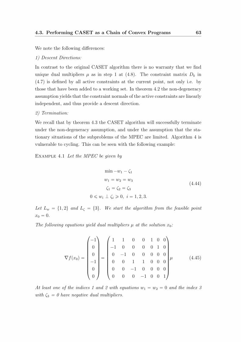
4.3. Performing CASET as a Chain of Convex Programs 63
We note the following differences:
1) Descent Directions:
In contrast to the original CASET algorithm there is no warranty that we find
unique dual multipliers µ as in step 1 at (4.8). The constraint matrix Dk in
(4.7) is defined by all active constraints at the current point, not only i.e. by
those that have been added to a working set. In theorem 4.2 the non-degeneracy
assumption yields that the constraint normals of the active constraints are linearly
independent, and thus provide a descent direction.
2) Termination:
We recall that by theorem 4.3 the CASET algorithm will successfully terminate
under the non-degeneracy assumption, and under the assumption that the sta-
tionary situations of the subproblems of the MPEC are limited. Algorithm 4 is
vulnerable to cycling. This can be seen with the following example:
Example 4.1 Let the MPEC be given by
min´w1 ´ ζ1
w1 “ w2 “ w3
ζ1 “ ζ2 “ ζ3
0 ď wi K ζi ě 0, i “ 1, 2, 3.
(4.44)
Let Lw “ t1, 2u and Lζ “ t3u. We start the algorithm from the feasible point
x0 “ 0.
The following equations yield dual multipliers µ at the solution x0:
∇fpx0q “
¨
˚
˚
˚
˚
˚
˚
˚
˚
˚
˝
´1
0
0
´1
0
0
˛
‹
‹
‹
‹
‹
‹
‹
‹
‹
‚
“
¨
˚
˚
˚
˚
˚
˚
˚
˚
˚
˝
1 1 0 0 1 0 0
´1 0 0 0 0 1 0
0 ´1 0 0 0 0 0
0 0 1 1 0 0 0
0 0 ´1 0 0 0 0
0 0 0 ´1 0 0 1
˛
‹
‹
‹
‹
‹
‹
‹
‹
‹
‚
µ (4.45)
At least one of the indices 1 and 2 with equations w1 “ w2 “ 0 and the index 3
with ζ3 = 0 have negative dual multipliers.

4.3. Performing CASET as a Chain of Convex Programs 64
Given the case that w1 “ 0 has a negative multiplier -1, by beginning with the
smallest index we might shift the index i “ 1 from Lw to Lζ. Given that ζ1 “ 0
has a negative multiplier -1 in the next iteration, we would end up in a cycle.
Even a simple anti-cycling rule that avoids the indices from past iterations can
fail (e.g. if we start with Lw “ t1, 3u and Lζ “ t2u we might receive the series
pt1, 3ut2uq Ñ pt3ut1, 2uq Ñ pt2, 3ut1uq Ñ pt2ut1, 3uq Ñ . . . ).
However, problem (4.44) is unbounded from below and x0 is not a strongly sta-
tionary point.
For the sake of completeness we want to state a rather simple fact that will be
used in combination with the BBASET algorithm.
4.5 Theorem
Every solution of problem (4.43) is an A-stationary point of the MPEC (4.42).
Proof We recall that x˚ “ py˚, w˚, ζ˚q is A-stationary (def. 2.10) if there exist
multipliers λ “ pλy, λw, λζqT such that:
0 “ ∇fpx˚q ` CTµ´ λ
λy ě 0
λyi “ 0, @i P ti | y˚i ą 0u
λwi “ 0, @i P I`0
λζi “ 0, @i P I0`
λwi ě 0 or λζi ě 0, @i P I00.
(4.46)
The conditions are now verified for the multipliers at a KKT-point x˚ of the
convex problem (4.43). Let the KKT-multipliers be denoted by pµ, λy, λw, λζq
as the multipliers in (4.46). Their existence is given by theorem 2.1 since (4.43)
satisfies the Abadie-CQ. They satisfy the first equation of (4.46) and further:
If i P Lw then i must be in I0` Y I00 and λwi free, λζi ě 0 and λζi ζi “ 0.
If i P Lζ then i must be in I`0 Y I00 and λζi free, λwi ě 0 and λwi wi “ 0.
It holds that λy ě 0 and yTλy “ 0.
By this we see that the multipliers also satisfy the conditions of system (4.46)
which proves that the KKT-point x˚ is A-stationary. �

4.3. Performing CASET as a Chain of Convex Programs 65
4.6 Theorem
Algorithm 4 will perform as in one of the three cases:
1. It will detect unboundedness or infeasibility of the MPEC after a finite
number of iterations,
2. or find a strongly stationary point after a finite number of iterations,
3. or end in a cycle of A-stationary points with the same objective value.
Proof If the algorithm ends after a finite number of iterations then it must have
terminated in step 1 which covers case 1 and 2.
Assume that algorithm 4 is interminable. There are only finitely many con-
stellations for the partitioning sets Lw and Lζ of t1, . . . ,mu and each problem
P pLw, Lζq in (4.43) has a unique minimal objective value. It holds that the solu-
tion xk at the k´ th iteration is feasible in the convex problem in iteration k` 1.
This yields a monotone (but not necessarily strictly monotone) descent in the
objective value. With the finite number of possible objective values and theorem
4.5 it follows that case 3 is present. �
With this theorem it follows that algorithm 4 is ready to be embedded into the
BBASET framework:
Remark 4.3 Algorithm 4 is finite if we terminate at a repeating constellation
of indices Lw and Lζ . The algorithm always yields an A-stationary point by
theorem 4.5.
With this modification the algorithm can be embedded into the BBASET branch-
and-bound framework with the extension to A-stationary points as in remark 4.2.
4.3.1. Anticycling and B-Stationarity
One can show that overcoming cycling in algorithm 4 can be related to a prob-
lem with linear objective function and linear complementarity constraints. The
problem of finding a feasible descent direction is given by:
4.3. Performing CASET as a Chain of Convex Programs 66
mind∇fpxqTd
Cd “ 0
di ě 0, @i P ti | xi “ 0u
dwi “ 0, @i P Lw X ti | ζi ą 0u
dζi “ 0, @i P Lζ X ti | wi ą 0u
dwi dζi “ 0, @i P ti | ζi “ wi “ 0u.
(4.47)
The set of constraints is the linearized MPEC tangent cone as in definition 2.8.
We note that (4.47) either has the solution 0 (which is always feasible), or the
problem is unbounded (since every solution ‰ 0 yields an unbounded ray).
Let x in (4.47) be the solution of the convex problem in some iteration of algo-
rithm 4. The task is to generate a disjunction of the indices ti | ζi “ wi “ 0u
with two sets Lw and Lζ such that the program
mind∇fpxqTd
Cd “ 0
di ě 0, @i P ti | xi “ 0u
dwi “ 0, @i P pLw X I0`q Y Lw
dζi “ 0, @i P pLζ X I`0q Y Lζ
(4.48)
is unbounded. In this case we have found updates of the working sets
Lw Ð pLw X I0`q Y Lw
Lζ Ð pLζ X I`0q Y Lζ(4.49)
that yield progress in algorithm 4. If the disjunction (Lw and Lζ) does not exist
then we have verified that no feasible descent direction exists and thus x is a B-
stationary point. In this sense finding Lw and Lζ is equivalent to solving (4.47).
The following algorithmic concept finds a solution of (4.47):
We start with the common simplex algorithm on system (4.47) without the com-
plementarity constraints. We assume the simplex algorithm is performed with
an anticycling strategy, e.g. the pivot rule of Bland [22]. Since d “ 0 is a feasible
4.4. Methodological Outlook 67
solution, we notice that any constellation of linearly independent columns of C
represents a basic solution which is suitable to begin with.
If we find an unbounded ray d with dwi ą 0 and dζi ą 0, we branch the problem
into two subproblems where one has the additional constraint dwi “ 0 and the
other has the additional constraint dζi “ 0. This can be done most conveniently
when determining the stepsize and the exiting basis index. We continue the
search on both branches, branching further if necessary.
This algorithm will eventually find that no non-zero direction which is feasible
in (4.47) exists, or the solution d shows an arrangement of indices such that
algorithm 4 can progress.
With this modification it holds that if algorithm 4 is started from a feasible
arrangement of indices, it will terminate with a B-stationary point (with remark
2.3) or prove that problem (4.42) is unbounded.
4.4. Methodological Outlook
The following chapter develops another component for the hybrid algorithm,
which will be presented in chapter 7. The hybrid algorithm incorporates the
techniques of the CASET algorithm in finding stationary points, and parts of
the BBASET algorithm in the branching steps. In the following, a method that
is originally designed to solve problems with linear objective function and linear
complementarity constraints, will be adapted and used to calculate points that
can be utilized as entry points for the CASET algorithm on the node problems
of the BBASET branches. It has been shown how the CASET algorithm can be
performed by solving a chain of convex problems. The design of the method in
the following chapter has the same key aspect, i.e. it can be performed by solving
a series of (convex) linear problems.
5. A Modification of the Algorithm of Hu et al.
This chapter focuses on a special subclass of MPECs that are linear programs
with linear complementarity constraints (LPCCs). LPCCs are closely related to
mixed integer programming, and can be encountered in the special case of bilevel
problems with linear upper level objective functions as in parameter identification
problems [8]. They can also be encountered in other applications such as e.g.
absolute value programming [30] or certain modeling techniques for the knapsack
problem [32]. For further information on these problems the reader is referred to
the given references. As was mentioned in section 2.3, many NLP approaches to
MPECs exists which can find solutions efficiently. These methods often have the
disadvantage of converging to lower class stationary points that are not locally
optimal. This chapter focuses on methods that solve the problems to global
optimality, especially the method of Hu et al. [24] for LPCCs.
Let the general linear complementarity problem (GLCP) be defined as in [19]:
Find py, ζq such that
q `Mζ `Ny ě 0
p`Rζ ` Sy ě 0
ζT pq `Mζ `Nyq “ 0
y, ζ ě 0
(5.1)
where ζ P Rn and y P Rl, M is a quadratic matrix and N , R and S are rectangular
real matrices and q and p real vectors, all of suitable dimensions. We note that
the GLCP is a special case of of an LPCC. Further, a special case of the GLCP
is the linear complementarity problem (LCP): Find pw, ζq P R2n such that
w “ q `Mζ
wT ζ “ 0
w, ζ ě 0.
(5.2)
68
5.1. The General Linear Complementarity Problem 69
The GLCP and LCP have been widely investigated as is shown in the first section,
and the LCP can be solved efficiently under certain assumptions for the matrix
M . In contrary the general case has shown to be NP-hard.
The algorithms that are presented at the end of this chapter will focus on the case
where no additional assumptions for the underlying linear constraints are made.
After an introduction, the method of Hu et al. will be modified for the task of
finding feasible points in a GLCP, where this GLCP corresponds to the feasible
area of an MPEC with convex objective function. The final algorithm uses the
information from a surrounding branch-and-bound procedure of the MPEC, and
a heuristic linear objective function in order to generate feasible points for the
nodes in the binary tree.
5.1. The General Linear Complementarity Problem
In [41] the so called unified interior point method is presented that is applied to
the LCP (5.2), where M is in the class of P0 matrices.
5.1 Definition (P0 Matrix, [21]) A matrix M is in P0 if and only if it is
quadratic and its principal minors are non-negative.
The k´ th principal minor of a matrix m “ pmijqi,j“i,...,n is defined as the deter-
minant of the submatrix pmijqi,j“1,...,kďn.
Remark 5.1
• We note that if M is positive definite then M is a P0 matrix.
• If the principal minors are strictly positive then M is called a P matrix.
The unified interior point method solves the QP
minwT ζ
w “ q `Mζ
w, ζ ě 0.
(5.3)
Under the assumption that
• M is in P0,

5.1. The General Linear Complementarity Problem 70
• a startpoint in the interior tpw, ζq | w “ q `Mζ, ζ ą 0u of the feasible
region is available and
• the objective function wT ζ of the QP is bounded on the level sets tpw, ζq|w “
q `Mζ, ζ ě 0, wT ζ ď tu
it holds that the method finds a point with objective value 0, which is a solution
to the LCP, in polynomial time. This does not hold for the GLCP as it has
been shown to be NP-hard if M is positive semi-definite (PSD) (see [33] and the
references therein).
In order to evaluate the computational complexity, minor assumptions are made,
e.g. the matrix M is required to have rational entries. One class of matrices
where all requirements are fulfilled, are row sufficient matrices:
5.2 Definition (RS Matrix, [11]) A matrix M is called row sufficient (RS)
if
xTi pMTxqi ď 0, @iñ xTi pM
Txqi “ 0, @i. (5.4)
We return to the GLCP (5.1) with the additional requirement that R “ 0. The
monograph [19] gives a strong impression, of how a number of different non-
convex programs in bilevel programming are related to each other. They show
that by introducing suitable surplus variables and a merit function, the GLCP
can be encountered by solving an NLP.
5.1 Theorem ([19] Thm. 1)
Let the GLCP be given by
w “ q `Mζ `Ny
v “ p` Sy
wT ζ “ 0
ζ, y, w, v ě 0.
(5.5)
If the feasible area is nonempty and M is an RS matrix, then any stationary
point of the NLP
min }w ´ q ´Mζ ´Ny}2 ` }v ´ p´ Sy}2 ` pÿ
i
pζiwiqgqh
(5.6)

5.1. The General Linear Complementarity Problem 71
ζ, w, y, v ě 0 (5.7)
where g, h ě 1 and g ą 1 if h “ 1, is a solution of the GLCP.
Now that a solution method for this case has been established, it is possible to
convert bilinear programming problems (BLPs) and LCPs into a form, to which
the NLP approach can be applied.
A BLP is defined by
min cTx` dTy ` xTHy
Ax ě a
x ě 0
By ě b
y ě 0
(5.8)
where H is a general rectangular matrix. Finding a stationary point for this
problem is considered NP-hard.
5.1 Lemma ([33])
The BLP can equivalently be restated as
min aTu` dTy
w1 “ c´ ATu`Hy
w2 “ ´a` Ax
v “ b´By
w1, w2, v, x, y, u ě 0˜
w1
w2
¸T ˜
x
u
¸
“ 0.
(5.9)
Proof Then transformation can be acquired by the formulation with two nested
problems
minytdTy `min
xtpx`HyqTx : x P Kxu : y P Kyu
Kx :“ tx| Ax ě a, x ě 0u
Ky :“ ty| By ě b, y ě 0u.
(5.10)

5.1. The General Linear Complementarity Problem 72
Since the inner problem is a standard LP, we may exchange it with its KKT-
conditions which are necessary and sufficient. �
The constraint matrix which connects the complementary vectors is
˜
0 ´AT
AT 0
¸
(5.11)
hence the BLP has been converted into a GLCP with PSD matrix and linear
objective function. One of the major applications of the BLPs, is finding integer
solutions with a non-convex quadratic objective. This is due to the fact that
every feasible point x in
Ax`By ě b
y ě 0
xi P t0, 1u
(5.12)
is a solution of the program
minxT pe´ xq
Ax`By ě b
0 ď x ď e
y ě 0
(5.13)
with an objective function value of 0, where e is a vector of ones. An important
application for this conversion is the so called knapsack problem [54, 39, 53]:
min cTx
aTx “ b
x P t0, 1un.
(5.14)
For the LCP (5.2) there exists a conversion to a BLP that uses additional vari-
ables.
5.2 Lemma ([19])
The LCP (5.2) is equivalent to the BLP
5.1. The General Linear Complementarity Problem 73
min eT ζ ` qTx` xT pM ´ Iqζ
Mζ ` q ě 0
0 ď x ď e
ζ ě 0
(5.15)
where I is the identity matrix. A point pw, ζq is a solution of the LCP (5.2) if
and only if there exists a solution pζ, xq of the BLP (5.15) with objective value 0.
Proof The objective function in (5.15) is non-negative for every feasible point
of the BLP. For each complementary pair qi ` pMζqi and ζi exists a variable xi,
that ranges from 0 to 1. The case where wi ą 0 corresponds to xi “ 0 and the
case where qi ` pMζqi ą 0 corresponds to xi “ 1. The so called degenerate case
where both are zero is associated with the complete interval xi P r0, 1s. �
Judice et al. propose an algorithm that investigates this quadratic program on
a binary tree, fixing a variable xi to 0 or 1 at each branching step, until a global
optimum is found. For details on this see [32].
The BLP (5.15) can be transformed into a GLCP with linear objective function,
as seen before:
min eT ζ ´ eTu
w “ q ` u` pM ´ Iqζ
β “ e´ x
α “ q `Mζ
α, ζ, w, β, x, u ě 0
xTw “ uTβ “ 0.
(5.16)
As a last step in transforming the problem, in [19] Fernandes et al. introduce
another positive variable γ0 “ eT z ´ eTu that is equal to the objective function.
Furthermore they introduce a positive variable λ0 such that
β “ e´ x´ λ0e. (5.17)

5.1. The General Linear Complementarity Problem 74
It follows that if λ0 ă 1 then xi ` βi ą 0, @i “ 1, . . . , n and
pβi ‰ 0^ ui “ 0q _ pxi ‰ 0^ wi “ 0q, @i “ 1, . . . , n. (5.18)
5.2 Theorem ([19] Thm. 2)
Let a reformulation be given by
w “ q ` u` pM ´ Iqζ
β “ e´ x´ λ0e
γ0 “ eTu´ eT ζ
α “ q `Mζ
α, ζ, w, β, γ0, x, u, λ0 ě 0
xTw “ uTβ “ λ0γ0 “ 0.
(5.19)
If the feasible set of the original LCP (5.2) is nonempty and (5.19) has a solution
pα˚, ζ˚, w˚, β˚, γ˚0 , x˚, u˚, λ˚0q where λ˚0 ă 1, then pζ˚, w˚q is a solution of the LCP
(5.2). Further it holds: There exists at least one solution where λ˚0 ď 1.
A remark on the two different cases under the condition λ0 ă 1 has been noted
in (5.18). See [19] for the complete proof.
Theorem 5.2 prepares for the following idea: The constraint matrix connecting
the complementary variables pw, β, γ0q and px, u, λ0q is
¨
˚
˝
0 I 0
´I 0 ´e
0 eT 0
˛
‹
‚
(5.20)
and hence positive semi-definite. Thus the NLP approach in theorem 5.1 can be
applied. With the merit function it is suggested to efficiently generate a number
of solutions of the program, until a solution with λ0 ă 1 is found.
5.1.1. A Pivoting Algorithm for LPCCs
Another approach is presented in the monograph [18] by Fang et al. In their
approach, the simplex algorithm is extended to linear problems with linear com-
5.1. The General Linear Complementarity Problem 75
plementarity constraints (LPCCs). The difference to general programs with linear
complementarity constraints (GLCPs) is, besides the linear objective function,
that for a number of indices there exist pairs of affine linear constraints which
are complementary to each other.
minxPRn
fpxq
Ax ě b
0 ď Hx´ h K Gx´ g ě 0
(5.21)
One can imagine the algorithm as the simplex algorithm with a restriction, con-
cerning which index is allowed to leave the basis when performing a pivoting step.
This is done in a way that always keeps one of the complementary constraints in
the working set. Results are first presented under some beneficial assumptions:
• there are n linearly independent active constraints at every vertex and
• an initial feasible vertex is given.
In this case, since their problem is defined with inequality constraints, the dual
multipliers of the active constraints indicate whether there exists a feasible de-
scent direction at the current vertex. If the algorithm terminates at a vertex
where the minimal dual multiplier is non-negative, then this vertex is a strongly
stationary point. We recall that every local minimum is a strongly stationary
point of an LPCC under the MPEC-LICQ but the opposite is not the case in
general (thm. 2.5).
With this information it remains to investigate B-stationarity in the degenerate
case, i.e. if the MPEC-LICQ is not present. To handle this situation, Fang et
al. initially propose the application of an anticycling strategy which is similar to
Bland’s rule [18]. Since this method does not eliminate the problem completely,
it is necessary to use an additional cycling detection mechanism.
Another solution for this situation has been suggested in section 4.3 where Bland’s
rule is combined with a branching step, in case of, let us call it, interference of
the complementarity constraints.
The result presented in [18] is an algorithm that finds a local minimum or detects
infeasibility under certain conditions, and does not depend on the non-degeneracy
assumption.

5.2. The Method of Hu et al. 76
5.2. The Method of Hu et al.
Extending earlier work of Ibaraki [26, 27] and Jeroslow [28] the authors present
an integer-programming based algorithm for LPCCs. The main idea is based
on observations of the dual programs that are obtained by restricting all of the
complementarity constraints to either side. Under the assumption of certain con-
ditions, one can prove the existence of a large big-M type parameter that allows
the possibility to remodel the problem with 0-1 integer variables. However, the-
oretical results aim to keep the corresponding integer variables in the underlying
method without relying on these assumptions. The approach leads to a minimax
0-1 integer program that resembles the original problem. Finally the method uses
cut management and generation steps, for cuts that emerge from the dual linear
problems, and also includes concepts for feasibility recovery and cut sparsification
subroutines.
The main problem is defined in accordance to the monograph [24]:
minpx,yq
cTx` dTy
Ax`By ě f
0 ď y K pq `Nx`Myq ě 0,
(5.22)
where c P Rn, d, q P Rm and f are real vectors and A, B, M and N are real
matrices, all of suitable dimensions.
In order to show the complete picture, a formulation, with integer variables z P
t0, 1um and a (suggestively large) parameter θ as in [24], is introduced. The
program LP pθ, zq is defined as
minpx,yq
cTx` dTy
Ax`By ě f
Nx`My ` q ě 0
Nx`My ` q ď θz
y ě 0
y ď θpe´ zq.
(5.23)

5.2. The Method of Hu et al. 77
For the standard linear problem LP pθ, zq the dual program DLP pθ, zq always
exists and is given by:
maxλ,u˘,v
fTλ` qT pu` ´ u´q ´ θpzTu` ` pe´ zqTvq
ATλ´NTpu` ´ u´q “ c
BTλ´MTpu` ´ u´q ´ v ď d
λ, u˘, v ě 0.
(5.24)
In the following context the unboundedness of a minimization problem is iden-
tified with an objective value of ´8. In case of infeasibility the minimum is 8.
This is practiced in reverse analogy for the case of maximization.
5.3 Lemma
Let ZpLP pθqq be the set of z where LP pθ, zq is feasible. We note the following
relations between the three problems
minpLPCCq “ lim infθÑ8
minz
minLP pθ, zq “ lim infθÑ8
minzPZpLP pθ,zqq
maxDLP pθ, zq.
(5.25)
Proof For the first equation we note that the LPCC is infeasible if and only if
LP pθ, zq is infeasible for every θ and z. On the other hand if LPCC is unbounded,
then there exists a ray say r and corresponding integer vector zr, such that
lim infθÑ8 LP pθ, zrq goes to ´8.
For the second equation we note that minLP pθ, zq ‰ maxDLP pθ, zq if and only
if both programs are infeasible. �
As the following analysis shows, these problems are not necessarily needed to
develop the parameter free integer based approach. Instead we take a direct
approach with the following parameter free but z-dependent LP (as defined in
[24]):
5.2. The Method of Hu et al. 78
ϕpzq :“ maxλ,u˘,v
fTλ` qT pu` ´ u´q
ATλ´NTpu` ´ u´q “ c
BTλ´MTpu` ´ u´q ´ v ď d
λ, u˘, v ě 0
zTu` ` pe´ zqTv ď 0
(5.26)
ϕ0pzq :“ maxλ,u˘,v
fTλ` qT pu` ´ u´q
ATλ´NTpu` ´ u´q “ 0
BTλ´MTpu` ´ u´q ´ v ď 0
λ, u˘, v ě 0
zTu` ` pe´ zqTv ď 0
(5.27)
5.1 Proposition ([24] Prop. 2.2)
For any z P t0, 1um it holds that ϕ0pzq “ 0 if and only if the system
Ax`By ě f
pNx`My ` qqi “ 0 if zi “ 0
pNx`My ` qqi ě 0 if zi “ 1
yi “ 0 if zi “ 1
yi ě 0 if zi “ 0
(5.28)
is feasible.
Proof Every feasible point in p5.27q remains feasible under multiplication with
a positive factor. It follows that the feasible area of p5.27q is a convex cone with
the only possible extreme point 0. It follows that ϕ0pzq P t0,8u. The dual of
system p5.27q is
minx,y,t
0
Ax`By ě f
tz ě q `Nx`My ě 0
tpe´ zq ě y ě 0
t ě 0
(5.29)

5.2. The Method of Hu et al. 79
where t is the positive dual variable that originates from the constraint zTu` `
pe ´ zqTv ď 0. We see that any point px0, y0q is feasible in (5.27) if and only
if there exists a feasible point px0, y0, tq in (5.29). With strong duality in linear
programming we can conclude the following points:
1. If ϕ0pzq “ 8 then (5.29) is infeasible (for every t ě 0).
2. If on the other hand (5.29) is infeasible, then (5.27) is either infeasible or
unbounded. And since the point 0 is always feasible the second of those
options follows.
3. It holds that ϕ0pzq “ 0 if and only if (5.29) is feasible.
Here the combination of point 1 and 2, or point 3 by itself, are sufficient to verify
the proposition. �
In other words proposition 5.1 establishes a connection between the cone of un-
bounded rays of (5.26), and the feasibility of one convex subset of the solution
space of the original LPCC (5.22). The nature of this combinatorial problem is
captured in the integer vector z where each variable zi directly corresponds to
branching on the i-th complementarity constraint.
5.3 Definition (z-leaf) The feasible area of (5.28) that depends on z is lz and
is denoted a leaf or the z-leaf of problem (5.22). The program that emerges from
minimizing cTx` dTy on the feasible area lz shall be denoted LP pzq.
Remark 5.2 For a given vector z the dual program of system p5.26q, which
defines ϕpzq, is LP pzq.
For the main algorithm there will be repeated evaluations of ϕpzq for different
integer vectors z by solving (5.26). We take a closer look at the constraint
zTu` ` pe ´ zqTv ď 0 that has been used in the definition of ϕpzq. The term
initially appeared in the objective function of DLP pθ, zq and has then moved to
the set of constraints. Since z, pe´ zq, u` and v are non-negative, the constraint
yields
u`i “ 0 if zi “ 1
vi “ 0 if zi “ 0.(5.30)

5.2. The Method of Hu et al. 80
The variables u` and v are dual to the θ dependent constraints
Nx`My ` q ď θz and y ď θpe´ zq. (5.31)
in the system of LP pθ, zq. If our intention is that minz LP pθ, zq resembles a part
of the original LPCC (5.22) then the first of these constraints for index i is only
supposed to become active for zi “ 0, and the second is only supposed to become
active for zi “ 1. In all other cases the parameter θ has not been chosen big
enough. If they are not active then the corresponding duals are supposed to
become zero. The constraint zTu` ` pe´ zqTv ď 0 in (5.26) and (5.27) achieves
this effect.
Finally, in the same way as ϕ0 has been related to feasibility, ϕ can be related to
the leaves of the LPCC with remark 5.2:
1. If ϕpzq “ 8 then it follows that lz is infeasible.
2. If ϕpzq is finite then it is equal to the optimal value of LP pzq.
3. If ϕpzq “ ´8 (which means that (5.26) is infeasible) then with proposition
5.1 it follows that lz is infeasible if and only if ϕ0pzq “ 8, or else LP pzq is
unbounded.
The algorithm uses the results related to ϕpzq and ϕ0pzq. The main idea is
that every evaluation of ϕpzq yields either a feasible point for the LPCC, and
therefore an upper bound, or it yields an unbounded ray which means that lz is
infeasible. In the case where program (5.26) itself is infeasible, one can evaluate
ϕ0 to determine whether LP pzq is unbounded or infeasible. With the acquired
dual unbounded ray or point it is possible to introduce certain constraints on the
set of all z (which will later define the set Zwork Ď t0, 1um).
5.2.1. Extreme Point and Ray Cuts
Let us assume that ϕpz0q and ϕ0pz0q have been evaluated for an arbitrary but
fixed z0 P t0, 1um. Further assuming that the LPCC is not unbounded on lz0 ,
it follows that we have either found an extreme point pλ0, u˘0 , v0q of (5.26), or
an extreme ray of (5.27). These options correspond to a feasible point of the
LPCC or the infeasibility of lz respectively. In the second case it follows that

5.2. The Method of Hu et al. 81
pλ0, u˘0 , v0q ‰ 0. In order to ensure progress in the enumeration algorithm, con-
straints are introduced for the vector z that are provided by the following result.
5.4 Lemma ([24])
1. The point pλ, u˘, vq is feasible in (5.26) for z if and only if
ÿ
l:u`l ą0
zl `ÿ
l:vlą0
p1´ zlq “ 0.(5.32)
2. The ray pλ, u˘, vq ‰ 0 is feasible in (5.27) for z if and only if equation (5.32)
holds.
Assume that we are in the situation described above and have evaluated ϕpz0q
and ϕ0pz0q. Since every feasible z is an integer vector, the following constraint
can be deducted in both cases of lemma 5.4:
ÿ
l:u`l ą0
zl `ÿ
l:vlą0
p1´ zlq ě 1.(5.33)
5.2.2. Sparsification Procedure
The authors of [24] have developed a procedure that improves the cuts which can
be derived from lemma 5.4. A brief example illustrates the idea:
z1 ` z3 ` p1´ z6q ě 1
ô pz1 ` p1´ z6q ě 1 _ z3 ě 1q(5.34)
After the integer cut has been branched on, a resulting subcut can be verified by
information from the surrounding solution process. Let the cut be given by
ÿ
iPIzi `
ÿ
jPJp1´ zjq ě 1 (5.35)
where I and J are disjunct sets of indices. The cut can be sparsified by the
decomposition
ÿ
iPI1zi `
ÿ
jPJ1p1´ zjq ě 1 _
ÿ
iPI2zi `
ÿ
jPJ2p1´ zjq ě 1 (5.36)

5.2. The Method of Hu et al. 82
where I “ I1 Y I2 and I “ I1 Y I2. In order to verify the first subcut, a lower
bound is calculated for all the leaves which violate the subcut. The calculation
is based on a model derived from the primal formulation
LPrlx :“ minx,y
cTx` dTy
Ax`By ě f
pNx`My ` qqi “ 0 if i P I1
pNx`My ` qqi ě 0 if i R I1
yi “ 0 if i P J1
yi ě 0 if i R J1.
(5.37)
If this lower bound is greater than or equal to the objective function value of the
best currently known solution, then every leaf that violates the subcut is not of
interest for the global solution algorithm. It follows that the subcut can safely
be introduced to the working set and replace the original parent cut.
The sparsification of the cuts is embedded in the overall algorithm. Assume that
UB is the currently known upper bound. After the solution of problem (5.37)
the following three cases may occur [24]:
1. If the lower bound LPrlx ě UB and is relatively close to UB then further
sparsification might not be very promising. All the leaves that violate the
cut yield no improvement on the upper bound. The cut is added to the
current working system (Zwork).2. If the lower bound LPrlx ě UB and is even larger than UB ` δ for a given
constant parameter δ, then the cut is already useful but might be even more
useful if it is further sparsified. The cut is applied and marked for further
sparsification.
3. If the lower bound LPrlx ă UB then a feasibility recovery procedure is
started that can - if successful - yield a new feasible point for the LPCC and
therefore might yield an improvement of the upper bound. The feasibility
recovery procedure works with linear problems and can take advantage
of the particular structure of the problem instance. However, it is not
necessarily successful. If it fails then the cut can not yet be imposed and
its application is postponed. In this case it is added to a set Zwait.

5.2. The Method of Hu et al. 83
5.2.3. Main Algorithm
At this point we can state the main algorithm of [24] that finds a global solution
of the LPCC (5.22):
Step 0 (Initialization): Initialize the sets of generated cuts
Zwork “ Zwait “ H;
Initialize the solution space of z: Zwork “ t0, 1um;
Initialize the upper bound UB “ 8 and lower bound LB “ ´8;
Step 1 (Select z): Determine a vector z P Zwork. If Zwork “ H got to step
2, otherwise go to step 3;
Step 2 (Terminate): If no solution has been found until now, then the
LPCC is infeasible. Otherwise the solution with the lowest objective value
found so far is globally optimal - terminate;
Step 3 (Compute): Compute ϕpzq by solving (5.26). If ϕpzq is finite then
go to step 4a, if ϕpzq “ 8 go to step 4b, if ϕpzq “ ´8 go to step 4c;
Step 4a (Finite Solution): Decide on the following three cases:
1. If ϕpzq is relatively close to UB then add the corresponding point cut to
Zwork and continue;
2. If ϕpzq is reasonably larger then apply the sparsification procedure;
3. If ϕpzq ă UB then update UB Ð ϕpzq and continue;
Step 4b (Extreme Rays): The solution of (5.26) is an extreme ray.
Generate the cut and apply the sparsification procedure, update Zworkand Zwait accordingly;
Step 4c (Unboundedness): The LPCC might be unbounded in this case.
Solve (5.27) to compute ϕ0pzq. If ϕ0pzq “ 0 then the problem is
unbounded. Else if ϕ0pzq “ 8 then go to step 4b;
Step 5 (Apply this if the lower bound decreases): Move the waiting cuts
with LPrlx ą UB to Zwork since they are valid by now. Apply the
sparsification procedure to the new cuts;
Algorithm 5: The Main IP-based Algorithm [24]

5.3. Adaptation and Application of the Method 84
This finishes the section as the main algorithm is complete. The presented re-
sults have been selected so the algorithm can be developed in a brief and direct
theoretical approach. The authors of [24] present some additional results that
add to the main idea, but are not necessarily needed to build the theoretical
foundation. They have conducted computational experiments in comparison to
the NEOS solvers FILTER and KNITRO (https://neos-server.org/neos/),
for more details on the experiments the reader is referred to the original article
[24]. The next section shows the application and adaptation of this concept to
the feasibility of GLCPs with convex objective function.
5.3. Adaptation and Application of the Method
In the previous section we have seen the main algorithm of [24]. Now an adap-
tation of the algorithm is used to generate feasible points in a branch-and-bound
solution process for a general problem with convex objective function and com-
plementary variables:
minxfpxq
Cx “ Cyy ` Cww ` Cζζ “ g
x “ py, w, ζq ě 0
wT ζ “ 0.
(5.38)
where Cy P Rkˆl, Cw P Rkˆm, Cζ P Rkˆm and C “ pCy, Cw, Cζq are real matrices,
g P Rk and f : Rn Ñ R convex and n “ l ` 2m. As seen in the previous section,
we can identify the set t0, 1um with the leaves of the feasible area.
Remark 5.3 (lz for the MPEC (5.38))
The leaf lz is defined in accordance to the previous section. For z P t0, 1um the
leaf lz of problem (5.38) is the set defined by the following constraints
Cx “ g
x “ py, w, ζq ě 0
wi “ 0 if zi “ 0
ζi “ 0 if zi “ 1.
(5.39)

5.3. Adaptation and Application of the Method 85
In order to investigate the feasibility of these systems we take a look at the dual
problem of (5.39) with an added constant objective function.
5.5 Lemma
1) The dual problem DLP pzq for (5.39) with constant objective function exists
and is given by
max gTλ
CTy λ ď 0
pCTwλqi ď 0 if zi “ 1
pCTζ λqi ď 0 if zi “ 0.
(5.40)
2) The optimal objective value of DLP pzq is either 8 or 0.
3) Any unbounded ray in (5.40) remains an unbounded ray if we change the offset
to the point 0.
Proof 1) The dual program exists since the primal program is an LP. We receive
the problem
max gTλ
CTλ`ÿ
i: zi“0
µwp0, ei, 0qT`
ÿ
i: zi“1
µζp0, 0, eiqT“ 0 (5.41)
for unrestricted dual variables λ, µw and µζ . The dual variables µw and µζ are
redundant and so are the corresponding constraints. After elimination (5.40)
remains.
2) Any feasible point in (5.40) with positive objective value can be scaled infinitely
and remains feasible. Further it holds that the point 0 is feasible. Thus the
problem can only be unbounded, or the point 0 is optimal.
3) Follows from the arguments in 2). �
By normalizing the cone of unbounded rays of (5.40) with constant 1, we prepare
for the introduction of a heuristic objective function.
5.6 Lemma
For z P t0, 1um it holds that DLP pzq “ 8 and λ is an unbounded ray of (5.40) if
and only if there exists a number t ą 0 and a positive vector ν such that ν “ tλ
and ν satisfies the system

5.3. Adaptation and Application of the Method 86
gTν “ 1
CTy ν ď 0
pCTwνqi ď 0 if zi “ 1
pCζνqi ď 0 if zi “ 0.
(5.42)
Let us now assume that we have found z0 P t0, 1um such that DLP pz0q “ 8 and
a corresponding ray λ0 which means that the leaf lz0 is infeasible. We introduce
a cut which is constructed just as in the method of [24]:
CUT pλ0q :ÿ
i:pCTwλ0qią0
zi `ÿ
i:pCTζ λ0qią0
p1´ ziq ě 1. (5.43)
5.7 Lemma
1. Let λ0 be an unbounded ray in (5.40) for z0 P t0, 1um. It holds that λ0 is
an unbounded ray of (5.40) for z P t0, 1um if and only if:
z violates CUT pλ0q or (5.38) is infeasible.
Proof Let λ0 be an unbounded ray and without limitation we assume that λ0
satisfies (5.42). If pCTwλ0qi ą 0 or pCT
ζ λ0qi ą 0 for one i P t1, . . . ,mu and z
violates CUT pλ0q, then this is equivalent to zi “ 0 for every i where pCTwλ0qi ą 0,
and zi “ 1 for every i where pCTζ λ0qi ą 0. In consequence λ0 satisfies all the
constraints of (5.42) for z.
The other case is that CTwλ ď 0 and CT
ζ λ ď 0 holds regardless of any row indices.
Then for any z P t0, 1um it follows that λ satisfies (5.42). This is the case when the
inequality of the cut cannot be satisfied. The consequence is that lz is infeasible
for any z and thus (5.38) is infeasible. �
Keeping the idea of sparsification in mind, we see that the problem of finding
a vector λ that generates a cut with few entries, needs to consider the indices i
where pCTwλ0qi ą 0 and i where pCT
ζ λ0qi ą 0. In this sense the sparsest cut is
defined by the following MILP in relation to (5.42):

5.3. Adaptation and Application of the Method 87
minλ,τ
2mÿ
j“1
τj
gTλ “ 1
CTy λ ď 0
pCTwλqi ď τiθ for i “ 1, . . . ,m
pCTζ λqi ď τm`iθ for i “ 1, . . . ,m
τ P t0, 1u2m
pCTwλqi ď 0 if zi “ 1
pCTζ λqi ď 0 if zi “ 0
(5.44)
where θ is a large real number. There always exists θ0 such that for every θ ě θ0
the result does not depend on θ. To see this we note that the objective only
depends on τ , and τ is feasible if there exists λτ , such that pλτ , τq is feasible in
(5.44). Since the set of all τ P t0, 1u2m is finite, this yields a constant θ0.
Remark 5.4 We want to elaborate on program (5.44):
Let Cz “ pCy, pCwqti|zi“1u, pCζqti|zi“0uq be the matrix of columns which are avail-
able in the primal problem to present g as a positive linear combination. By
lemma 5.6, any feasible solution in program (5.44) proves that g does not lie
in the cone which is generated by these columns. Program (5.44) answers the
question of the maximal number of columns of C, that one can allow to be added
to Cz without letting g into the cone. A solution λ˚ of this problem can then be
translated to a constraint that forces at least one of the remaining columns to be
present in future calculations, i.e. a cut CUT pλ˚q is added to the set Zwork.
The use of system (5.44) in an algorithm is motivated by the following idea: Let
z be an integer vector that has been identified such that lz is infeasible. System
(5.44) generates a sparse cut that motivates the selection of another z and calls
the method again. If (5.44) turns out to be infeasible for some zk then the
corresponding leaf lzk is feasible as a result.
Since it might be relatively costly, solving a problem with integer variables τ is
avoided in later applications. Instead we solve the following linear problem that
does not necessarily yield the sparsest cut:

5.3. Adaptation and Application of the Method 88
minλ,τ
2mÿ
j“1
τj
gTλ “ 1
CTy λ ď 0
pCTwλqi ď τi for i “ 1, . . . ,m
pCTζ λqi ď τm`i for i “ 1, . . . ,m
τ ě 0
pCTwλqi ď 0 if zi “ 1
pCTζ λqi ď 0 if zi “ 0.
(5.45)
5.3.1. The Algorithm
This section presents an algorithm that uses the previous results. The environ-
ment for the task is any branch-and-bound algorithm that investigates a problem
(5.38) with a binary tree. The task is applied to a node in the tree where some
of the complementary variables have been fixed to either wi “ 0 or ζi “ 0. The
result is a point that is feasible in the subproblem that resembles the node.
We note that the general idea of the sparsification procedure of section 5.2.2 can
also be used for the general convex function f . Just as Hu et al. evaluate a
linear objective function to check on a sparser version of a cut, it is possible to
evaluate f in the corresponding relaxed problem. If the objective function value
of the cut violating relaxed problem is higher than the current upper bound in
a branch-and-bound step, then one can conclude that the sparser version of the
cut is eligible for the problem and the parent cut can be removed. In contrast to
the method of Hu et al. there will be no feasibility recovery approach after the
solution of the relaxed problem. Another aspect is that by using system (5.44)
or (5.45) the sparsification of the cut has already reached its target.
For two disjunct index sets Iw, Iζ Ă t1, . . . ,mu the node NpIw, Iζq is associated
with the problem
5.3. Adaptation and Application of the Method 89
minxfpxq
Cx “ g
wT ζ “ 0
x “ py, w, ζq ě 0
wi “ 0, @i P Iw
ζi “ 0, @i P Iz.
(5.46)
The relaxation of this problem without the complementarity constraints wT ζ “ 0
is denoted by NrelpIw, Iζq and provides a lower bound for the objective function
at the node NpIw, Iζq.
The set of the vectors z which are eligible for the node NpIw, Iζq shall be denoted
NzpIw, Iζq and is defined by
Nz :“ tz P t0, 1um|zi “ 0 if i P Iw, zi “ 1 if i P Iζu. (5.47)
Why this definition is reasonable can be seen most easily with the primal formu-
lation (5.39) or through the fact that these z P Nz correspond to the leaves lz
whose union forms the solution space of N .
We introduce a subroutine (algorithm 6) that finds a feasible point for the node
problem (5.46) or returns a message that marks the node for fathoming. We
assume the input of a point x0 when the task is started. This could be a point
that has been feasible for a parent node or some similar information. The point
is used to guide a heuristic in the selection of z. The resulting algorithm is
algorithm 6.
Remark 5.5 Since the set of valid z in the algorithm is finite, algorithm 6 ter-
minates with z P Nz such that lz is feasible or provides a certificate of infeasibility
for N . Termination occurs after solving a finite number of LPs.
5.3.2. Partial Feasibility
The algorithm can be extended in order to find a point that satisfies only some
of the complementarity constraints, but at potentially fewer iterations. Such a
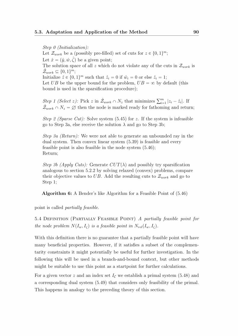
5.3. Adaptation and Application of the Method 90
Step 0 (Initialization):Let Zwork be a (possibly pre-filled) set of cuts for z P t0, 1um;
Let x “ py, w, ζq be a given point;The solution space of all z which do not violate any of the cuts in Zwork isZwork Ď t0, 1um;Initialize z P t0, 1um such that zi “ 0 if wi “ 0 or else zi “ 1;Let UB be the upper bound for the problem, UB “ 8 by default (thisbound is used in the sparsification procedure);
Step 1 (Select z): Pick z in Zwork XNz that minimizesřmi“1 |zi ´ zi|. If
Zwork XNz “ H then the node is marked ready for fathoming and return;
Step 2 (Sparse Cut): Solve system (5.45) for z. If the system is infeasiblego to Step 3a, else receive the solution λ and go to Step 3b;
Step 3a (Return): We were not able to generate an unbounded ray in thedual system. Then convex linear system (5.39) is feasible and everyfeasible point is also feasible in the node system (5.46);Return;
Step 3b (Apply Cuts): Generate CUT pλq and possibly try sparsificationanalogous to section 5.2.2 by solving relaxed (convex) problems, comparetheir objective values to UB. Add the resulting cuts to Zwork and go toStep 1;
Algorithm 6: A Bender’s like Algorithm for a Feasible Point of (5.46)
point is called partially feasible.
5.4 Definition (Partially Feasible Point) A partially feasible point for
the node problem NpIw, Iζq is a feasible point in NrelpIw, Iζq.
With this definition there is no guarantee that a partially feasible point will have
many beneficial properties. However, if it satisfies a subset of the complemen-
tarity constraints it might potentially be useful for further investigation. In the
following this will be used in a branch-and-bound context, but other methods
might be suitable to use this point as a startpoint for further calculations.
For a given vector z and an index set IC we establish a primal system (5.48) and
a corresponding dual system (5.49) that considers only feasibility of the primal.
This happens in analogy to the preceding theory of this section.

5.3. Adaptation and Application of the Method 91
minxfpxq
Cx “ g
x “ py, w, ζq ě 0
wi “ 0 if zi “ 0 and i R IC
ζi “ 0 if zi “ 1 and i R IC
(5.48)
The corresponding system for the generation of a dual unbounded ray in analogy
to (5.45) is
min2mÿ
j“1
τj
gTλ “ 1
CTy λ ď 0
pCTwλqi ď τi for i “ 1, . . . ,m
pCζλqi ď τm`i for i “ 1, . . . ,m
τ ě 0
pCTwλqi ď 0 if zi “ 1 or i P IC
pCζλqi ď 0 if zi “ 0 or i P IC.
(5.49)
The change to algorithm 6 happens mainly in Step 3b, the result is algorithm 7.
The extension of step 3b in algorithm 7 introduces dual constraints that are
equivalent to allowing the i-th column of Cw and Cζ both for the constraint matrix
of the primal system. As their presence in the problem with complementarity
constraints is mutually exclusive by the nature of the problem, these additional
constraints in the dual formulation correspond to a relaxation in their primal
counterpart. With this we reduce the complexity of the problem that originates
from its combinatorial nature, but receive only a partially feasible point in return.
Generally, this point yields neither an upper bound nor a lower bound for the
current node.
The focus on relaxation and reduction of iterations - in contrast to the feasibility
of the complementarity constraints - can be regulated by introducing or not
introducing the new constraints in step 3b of the algorithm. For computational

5.3. Adaptation and Application of the Method 92
Step 0 (Initialization):Initialize the algorithm in the same way as algorithm 6;Initialize a set of temporary constraints C “ H and a set of indicesIC “ H;
Step 1 (Select z): Pick z in Zwork XNz that minimizesřmi“1 |zi ´ zi|. If
Zwork XNz “ H then the node is marked ready for fathoming and return;
Step 2 (Sparse Cut): Solve system (5.49) with additional constraints C forz. If the system is infeasible go to Step 3a, else receive the solution λ andgo to Step 3b;
Step 3a (Return): We were not able to generate an unbounded ray in thedual system. Then convex linear system (5.48) is feasible and everyfeasible point is also feasible in the node system (5.46) if C and IC areempty. Otherwise the point might possibly violate the complementarityconstraints for the indices IC and is partially feasible;Return;
Step 3b (Apply Cut): Generate CUT pλq and possibly try sparsificationanalogous to section 5.2.2 by solving relaxed (convex) problems, comparetheir objective values to UB. Add the resulting cuts to Zwork and go toStep 1;
In Step 2 (Possibly add constraints to the set C): For a selected indexi P t1, . . . ,mu possibly add the two constraints pCT
wλqi ď 0 andpCT
ζ λqi ď 0. In this case also add the selected index i to IC;
Algorithm 7: A Bender’s like Algorithm for a Partially Feasible Point of (5.46)
experiments an input parameter is added, a kind of threshold, that marks the
inner iteration from which the relaxation is started and limits the number of
indices which enter the set IC in one progression. This parameter will later be
referred to in chapter 8 where numerical results are evaluated.
5.3.3. Intermediate Computational Results
Subroutine (algorithm) 6 has been embedded in an exemplary branch-and-bound
algorithm that finds the global optimum of (5.38) in a finite number of steps.
The branch-and-bound algorithm works like the BBASET algorithm, and uses
5.3. Adaptation and Application of the Method 93
algorithm 6 as a subroutine to generate feasible points. Algorithm 6 on the
other hand manages the cuts in Zwork and the corresponding set of valid integer
solutions z which is Zwork. In case of sparsification as in the method of Hu et al.
there might also be a set Zwait. The algorithm has an input parameter Imax that
is the maximum number of iterations in one call of algorithm 6.
Computational results with a first implementation have shown that many itera-
tions might otherwise be needed, depending on the specific instance, of course. If
the maximum number of iterations is breached, then the binary tree is expanded
by most infeasible branching with the information at hand instead of BBASET.
The result is algorithm 8.
Test instances have been created from the reweighting bilevel problem in chapter
3. The objective function is quadratic and convex, and the number of comple-
mentarity constraints ranges from 40 to 80. For a detailed description of the
instances the reader is referred to chapter 8 where the selection of the data is
described. Algorithm 8 has been compared to the Cplex MIQP solver. Consider-
ing calculation times for these rather small instances, it has been observed that
Cplex takes a clear lead. Solver iterations and nodes have also been recorded.
The CASET subroutine in algorithm 8 is performed by a series of convex prob-
lems, as described in section 4.3, where the convex QPs are solved by Cplex.
The relaxed programs are solved with the same instance of Cplex. A solve call is
recorded for each convex problem. The integer and LP programs of subroutine
algorithm 6 are also performed by individual instances of Cplex. We note that
algorithm 8 is designed for a general convex objective function f . The results are
presented in table 5.1 and 5.2. The differences, marked by 4, in table 5.1 indi-
cate that the corresponding value of the Cplex experiment has been subtracted
in this column. The number of solve calls has been compared to the number of
nodes in the Cplex MIQP solver. Other columns that are not marked by 4 state
the original values. The results have been generated with an Intel-i7 CPU, Cplex
version 12.1, Gurobi version 7.0 on a Dell notebook, code in Visual-C# 2013.

5.3. Adaptation and Application of the Method 94
Step 0 (Initialization):Initialize the set of generated cuts Zwork “ H;
Initialize the solution space of z: Zwork “ t0, 1um;Initialize the upper bound UB “ 8 and lower bound LB “ ´8;Initialize the set of active nodes N “ tNpH,Hqu;Get an input parameter ε ą 0;Get an input parameter Imax P NY t8u;
Step 1 (Termination): Update LB Ð mintLBpNq|N P N u;If UB ´ LB ď ε or |N | “ 0 then terminate;
Step 2 (Select Node): Select the current node N “ NpIw, Izq from N andremove it from the set;
If Nz X Zwork “ H then go to step 1;
Step 3 (Node Lower Bound): Solve the relaxed system Nrel;if the system is infeasible then
Go to step 1;else
Receive a solution xlb “ pylb, wlb, ζ lbq and a lower bound LBpNq for N ;endIf UB ´ LBpNq ď ε then go to step 0;
Step 4 (CASET): Load a feasible point x0 from the closest parent node;if x0 is feasible in the system of N then
Step 4a: Initialize CASET with x0;Let the resulting point be x˚ and store it in memory for the node N ;Update UB Ð mintUB, fpx˚qu;Generate new nodes from the strongly stationary point x˚ as inBBASET;
elseStep 4b: Call algorithm 6 with Zwork, UB and a maximum of Imax
iterations for the node N ;
On success: Receive z and update x0 Ð argminLP pzq;Go to Step 4a;
On infeasibility: Infeasibility of N has been confirmed, go to step 1;
On maximum iterations reached (Most infeasible branching): Get themost infeasible index j “ argmaxtwlbi ζ
lbi | i “ 1, . . . ,mu;
Create new nodes N1 “ NpIw Y tju, Iζq and N2 “ NpIw, Iζ Y tjuq;Update N Ð N Y tN1, N2u;
end
Step 5 (Loop): Go to Step 1;
Algorithm 8: A Branch-and-Bound Algorithm

5.3. Adaptation and Application of the Method 95
Solve SolverData Set s Obj. 4 Iterations Calls 4 Iterations 4 Time MIPs LPs Use MIPs?Data Set 1 20 0 50 2 926 5,71 626 572 yData Set 1 20 0 1181 1110 48119 1,87 0 0 nData Set 1 40 0 364 770 61952 27,95 2770 1503 yData Set 1 40 0 1559 621 73712 8,45 0 0 nData Set 2 20 0 32 -26 -354 2,55 366 328 yData Set 2 20 0 113 35 102 0,15 0 0 nData Set 2 40 0 761 1657 61731 21,46 2597 1133 yData Set 2 40 0 1105 962 52345 4,55 0 0 nData Set 3 20 0 6 8 -34 0,76 163 152 yData Set 3 20 0 19 10 228 0,04 0 0 nData Set 3 40 0 101 196 6396 1,91 305 127 yData Set 3 40 0 197 120 6399 0,78 0 0 nData Set 4 20 0 14 5 27 0,08 14 0 yData Set 4 20 0 23 5 -176 0,05 0 0 nData Set 4 40 19E-4 86 503 10619 8,11 1128 654 yData Set 4 40 19E-4 135 34 2251 0,34 0 0 n
Table 5.1.: Performance of Algorithm 8 on a small Test Set
• s - size parameter of targets in the reweighting lower level problem, the
number of complementarity constraints is 2s (see section 8.3);
• Objective 4 - difference between the objective values of the solutions of
algorithm 8 and the Cplex MIQP solver;
• Iterations - iterations of algorithm 8;
• Solve Calls 4 - difference between number of calls to the convex QP solver
(Cplex) in algorithm 8 and Cplex MIQP nodes;
• Solver Iterations 4 - difference between number of inner iterations of the
QP solver in algorithm 8 and iterations in the Cplex MIQP solver;
• Time - time in seconds;
• MIPs/LPs - number of calls to the integer/LP solver in algorithm 6;
• Use MIP-Appr - whether subroutine 6 was used or only most infeasible
branching was performed. In the second case the maximal number of iter-
ations Imax in step 3b is set to 0.
It has been observed that in few cases the number of nodes in the binary tree
was reduced, which was a main goal of performing this method. Calculation
times for the MIP approach are generally higher, which might be due to the
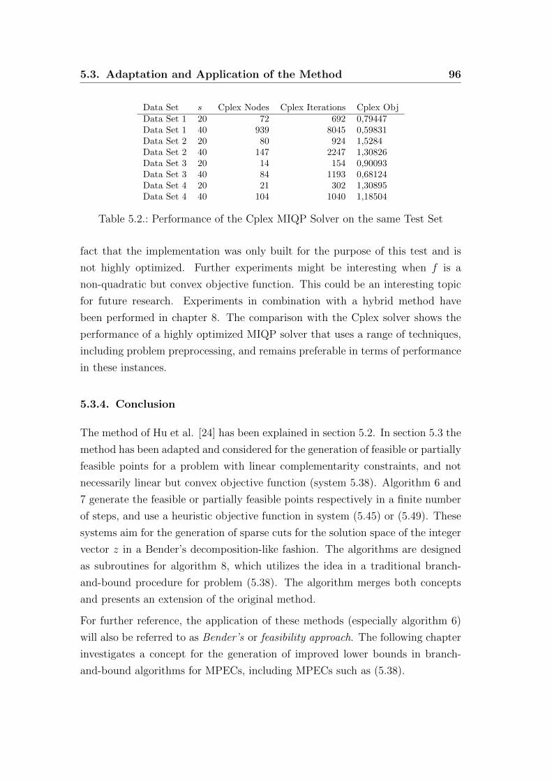
5.3. Adaptation and Application of the Method 96
Data Set s Cplex Nodes Cplex Iterations Cplex ObjData Set 1 20 72 692 0,79447Data Set 1 40 939 8045 0,59831Data Set 2 20 80 924 1,5284Data Set 2 40 147 2247 1,30826Data Set 3 20 14 154 0,90093Data Set 3 40 84 1193 0,68124Data Set 4 20 21 302 1,30895Data Set 4 40 104 1040 1,18504
Table 5.2.: Performance of the Cplex MIQP Solver on the same Test Set
fact that the implementation was only built for the purpose of this test and is
not highly optimized. Further experiments might be interesting when f is a
non-quadratic but convex objective function. This could be an interesting topic
for future research. Experiments in combination with a hybrid method have
been performed in chapter 8. The comparison with the Cplex solver shows the
performance of a highly optimized MIQP solver that uses a range of techniques,
including problem preprocessing, and remains preferable in terms of performance
in these instances.
5.3.4. Conclusion
The method of Hu et al. [24] has been explained in section 5.2. In section 5.3 the
method has been adapted and considered for the generation of feasible or partially
feasible points for a problem with linear complementarity constraints, and not
necessarily linear but convex objective function (system 5.38). Algorithm 6 and
7 generate the feasible or partially feasible points respectively in a finite number
of steps, and use a heuristic objective function in system (5.45) or (5.49). These
systems aim for the generation of sparse cuts for the solution space of the integer
vector z in a Bender’s decomposition-like fashion. The algorithms are designed
as subroutines for algorithm 8, which utilizes the idea in a traditional branch-
and-bound procedure for problem (5.38). The algorithm merges both concepts
and presents an extension of the original method.
For further reference, the application of these methods (especially algorithm 6)
will also be referred to as Bender’s or feasibility approach. The following chapter
investigates a concept for the generation of improved lower bounds in branch-
and-bound algorithms for MPECs, including MPECs such as (5.38).
6. Lower Bounds from Weak Duality
This chapter investigates the calculation of lower bounds that can be derived from
the Lagrange function. Lagrangian bounds have been the subject of research in
the field of global and discrete optimization [66, 23, 7, 17]. An algorithm with
Lagrangian bounds for programs with equilibrium constraints can be found in
[1]. The authors show that lower bounds can be calculated by a convex program
if the situation consists of variational inequality constraints with a positive semi-
definite constraint matrix [1, lemma 3.1].
The problems of this chapter satisfy no such conditions for the linear constraints,
and involve a number of positive complementary variables. We further develop
an algorithm that uses the branching techniques of the BBASET algorithm and
uses the new lower bounds. Let the problem P be defined as
minxfpxq
Ax “ b
gpxq ď 0
xixj “ 0 and xi, xj ě 0 @pi, jq PM Ď t1, . . . , nu2
(6.1)
where f : Rn Ñ R, A P Rlˆn and g : Rn Ñ Rk. The feasible set shall be denoted
by X and we assume that the minimum minpP q ą ´8 exists. Further, let f and
g be convex.
Define the subset XC :“ tx P X| xixj “ 0 and xi, xj ě 0 @pi, jq P Mu, and let
the Lagrange function L be defined only for the non-complementarity constraints
gpxq ď 0 and Ax “ b in the following sense:
Lpx, λ, νq :“ fpxq `kÿ
i“1
λigipxq `lÿ
j“1
νjpb´ Axqj
Lpλ, νq :“ infxLpx, λ, νq.
(6.2)
97
6.1. Lower Bounds from Weak Duality 98
If λ ě 0 it holds that
Lpx, λ, νq ď fpxq, @x P X, @ν P Rl. (6.3)
From this we conclude the following weak duality inequality:
Lpλ, νq ď infxPXC
Lpx, λ, νq ď infxPX
Lpx, λ, νq ď minxPX
fpxq “ minpP q (6.4)
The lower bound infxPXC Lpx, λ, νq can be greater than the relaxation of the
complementarity constraints. The relaxed program for P is given by
minxfpxq
Ax “ b
gpxq ď 0
xi, xj ě 0, @pi, jq PM.
(6.5)
Example 6.1
minw,ζě0
pw ´ 2q2 ` pζ ´ 2q2
w ` ζ “ 1
wζ “ 0
A strongly stationary point is p1, 0q with an objective value of 5.
Investigating optimality conditions at the point pw, ζq “ p1, 0q yields dual multi-
pliers pν, λw, λζq:
∇f “˜
2pw ´ 2q
2pζ ´ 2q
¸
˜
´1
´4
¸
` ν
˜
1
1
¸
` λw
˜
1
0
¸
` λζ
˜
0
1
¸
“ 0.
(6.6)
One solution is pν, λw, λζq “ p4,´3, 0q.

6.2. Remarks on Convex Analysis 99
The Lagrange lower bound for ν “ 4 is:
infw,ζě0,wζ“0
Lpw, ζ, 4q “ infw,ζě0,wζ“0
pw ´ 2q2 ` pζ ´ 2q2 ` 4p1´ w ´ ζq “ 5 (6.7)
where the relaxed problem
minpw ´ 2q2 ` pζ ´ 2q2
w ` ζ “ 1
w, ζ ě 0
(6.8)
yields a solution of pw, ζq “ p0.5, 0.5q and a lower bound of 4.5.
A problem is that in many cases the value of infxPXC Lpx, λ, νq is ´8. The
following theoretical observations belong to the field of convex analysis, and aim
to characterize the situations where infxPXC Lpx, λ, νq is unbounded below.
6.2. Remarks on Convex Analysis
In this section we consider f to be any convex function. Later a connection will
be established where f is the Lagrange function that is used in calculating a lower
bound, as seen above. The results aim to characterize the existence of a ray of
infinite descent of the function Lpx, λ, νq in XC for fixed vectors λ and ν.
We assume that f : Rn Ñ R is a proper convex function in the sense that
Dx0 P Rn : fpx0q ă 8
and fpxq ą ´8, @x P Rn.(6.9)
A direction that allows for unbounded descent lies in the cone of recession.
6.1 Definition (Direction of Recession, [61]) The vector s P Rn is called
a direction of recession of f if fpx ` tsq is a non-increasing function of t P R,
@x P Rn. The set of these directions 0`f is denoted the cone of recession.
The boundedness or unboundedness of such directions can be related to the ex-
istence of other directions of this kind. A number of results have already been

6.2. Remarks on Convex Analysis 100
established. A half-line tx ` td| t ě 0u (or the direction of it) is said to be
bounded or unbounded below, if fptx ` td| t ě 0uq is bounded or unbounded
below respectively.
6.1 Theorem ([61] 2.1)
1. If the half-line tx ` td| t ě 0u is unbounded below then so is any half-line
with direction d.
2. Any half-line with a direction in the relative interior of 0`f is unbounded
below.
3. If the direction is bounded below for one initial point then it is bounded
for any initial point.
Another theorem and following corollary limit the number of possible situations
for the boundary of 0`f .
Corollary 6.1 ([61] 2.2)
Let F be a face of 0`f , then
• either all s P F are directions of boundedness,
• or every s P rintpF q is a direction of unboundedness,
where rint denotes the relative interior.
Example 6.1 Let fpx, y, zq “ ´x be defined on R3. Then 0`f “ td| dx ě 0u.
It follow that there is exactly one face F “ td| dx “ 0u and the situation fits the
first case of corollary 6.1.
Further observations regard the existence of unbounded directions, beginning
with a lemma for the case of differentiable functions.
6.1 Lemma ([61] 2.3)
Let f : Rn Ñ R be convex and differentiable. Let d be a non-zero direction and
x P R, then it holds that
if limtÑ8
dT∇fpx` tdq ă 0
then d is an unbounded direction for every initial point.

6.2. Remarks on Convex Analysis 101
The following theorem establishes a tool for the existence and construction of an
unbounded direction for a convex function that is unbounded below.
6.2 Theorem
Let O be an open convex set and f be a proper convex function on O. Let pxnqnPN
be a sequence in O such that infnPN fpxnq “ ´8. Let x0 be any arbitrary point
in O. Then any accumulation point d of the directions dn “ pxn ´ x0q{}xn ´ x0}
is unbounded below if
lim supnÑ8
fpxnq
tanαn}xn ´ x0}“ ´8 (6.10)
where αn denotes the angle between dn and d.
Proof For each element xn let rn be the corresponding half-line, such that
rnptq :“ x0 ` tpxn ´ x0q, t ą 0. (6.11)
Since the unit sphere around x0 is a compact set it follows that the sequence
dn “xn´x0}xn´x0}
has at least one accumulation point that shall be denoted d. Let r
be the corresponding half-line with direction d and initial point x0.
For a small number ε ą 0 define
Q :“ clptx | Dn P N : px´ x0qTdn “ 0 and }x´ x0} “ εuq (6.12)
where cl denotes the closure. Since ε can be chosen arbitrarily small we find ε,
such that Q lies in the open set O.
For any element xn of the sequence it follows that there exists a line segment ln
that connects xn and Q, ln Ă O and also intersects r. The point of intersection
shall be denoted by yn P r. The connecting point in Q shall be denoted qn and
we choose qn such that dTn pqn ´ x0q “ 0. Further, αn is the angle between rn and
r by definition.
Since Q is closed and bounded we find that f is bounded from above on Q. There
exists λ such that yn “ λxn ` p1´ λqqn and λ satisfies the relations

6.2. Remarks on Convex Analysis 102
Figure 6.1.: Geometric Argument in Theorem 6.2
sinαn “ p1´ λq}qn ´ x0}
cosαn “ λ}xn ´ x0}.(6.13)
Using the convexity of f we conclude that
fpynq ď fpxnqλ` fpqnqp1´ λq
ďfpxnq
tanαn}xn ´ x0} ` }qn ´ x0}` fpqnq sinαn
}yn ´ x0}
qn ´ x0
.
(6.14)
Since yn P r it follows that r is unbounded below. �
Quadratic Problems
In the special case of quadratic functions the directions of recession are well
known. Let f be the quadratic function xTQx ` cTx where Q is positive semi-
definite. Further, let there be only linear constraints, which means we ignore the
constraint function g for now. Then the Lagrange function is
Lpx, νq “ xTQx` cTx`ÿ
j
νjpb´ Axqj. (6.15)

6.3. Application 103
If a leaf l satisfies the conditions of corollary 6.2 then there exists a direction of
infinite descent d that satisfies the following system of equations:
Qd “ 0
dl “ 0
Ad “ 0
cTd` νTd “ ´1
d ě 0.
(6.16)
On the other hand: If and only if d and l exist then the lower bound for the dual
vector ν is ´8.
6.3. Application
Consider problem (6.1) and the lower bound infxPXC Lpx, λ, νq for fixed λ and ν
where λ ě 0. We further assume that f is convex in a convex open set around
the feasible area, without the complementarity constraints. In the context of a
branch-and-bound procedure that works on the complementary indices in M , a
fixation of xi “ 0 or xj “ 0 for each of the complementary pairs pi, jq P M shall
be denoted a leaf. This definition is equivalent to the definition of a leaf in the
previous chapter. The constraints are gathered in the equation xl “ 0 where xl
denotes the corresponding subvector of x.
Corollary 6.2
The Lagrange lower bound Lpλ, νq, for λ ě 0 and ν fixed, is ´8 if a leaf l exists,
and a sequence in the feasible area of l such that the requirements of theorem 6.2
are satisfied. Then a direction of infinite descent in the feasible area of l exists
(from any initial point).
The corollary follows directly from the construction of the direction in the proof
of the theorem, and the fact that the feasible area without the complementarity
constraints is a closed convex set.

6.3. Application 104
A Model Algorithm
The efficient solution to the problem
infxPXC
Lpx, λ, νq (6.17)
is the key to utilizing these lower bounds. We notice that if BBASET is ap-
plied to this problem class, the issue of finding a feasible point to reinitialize the
CASET algorithm is not an issue, since the only constraints involved are the
complementary variable constraints.
The idea of algorithm 9 shows how the techniques are involved in calculating a
lower bound for problem (6.1) in a branch-and-bound setup. The key idea of the
algorithm is
1. that the investigation of a binary branch-and-bound tree of the complemen-
tarity constraints with an algorithm like BBASET is performed to gain a
good upper bound;
2. the investigation of the same binary tree with (6.17) (for any dual vector
pλ, νq with λ ě 0) yields lower bounds;
3. the calculation of (6.17) can be performed by BBASET without the issue
of finding feasible points to reinitialize CASET;
4. if the objective function is quadratic, then (6.16) yields a criterion for the
cases where (6.17) takes on the value ´8.
For a set of indices
L Ď ti | Dj : pi, jq PM or pj, iq PMu (6.18)
we let NL be the node that is defined by the additional constraints xL “ 0.
6.3. Application 105
Step 0 (Initialization):
Initialize D “ H the set of dual vectors;
Initialize N “ tNHu, the node set containing the root node and select
NL “ NH;
Initialize UB “ 8 and LB “ ´8 the upper and lower bounds of the
problem;
Step 1 (CASET): Process the selected node NL i.e. by calculating a
strongly stationary point x˚ with CASET;
Update UB Ð mintUB, fpx˚qu;
Add the vector pλ˚, ν˚q of dual multipliers from the solution to D;
Apply the lower bound
LBpNLq :“ suppλ,νqPD
infxPXC ,xL“0
Lpx, λ, νq (6.19)
to the selected node;
Step 2 (Directions of Infinite Descent): Identify directions of infinite
descent of Lpx, λ, νq, pλ, νq P D on leaves l1, . . . , ln in NL;
Solve a number of corresponding convex problems Nl, update UB and
expand D in the progress, with the aim that LBpNLq ą ´8;
Calculate LBpNLq by applying BBASET for a subset of D;
Step 3 (Branching and Termination): Update LB as the minimum of
LBpNq, N P N ;
if fpx˚Lq ´ LBpNLq ą ε thenBranching: Generate a number of subnodes from NL (i.e. BBASET)
and add them to N ;
end
if UB ´ LB ă ε then
Terminate ;
else
Select another node NL from N and go to step 1;
end
Algorithm 9: A Branch-and-Bound Algorithm with Lower Bounds from Weak
Duality
6.4. Conclusion 106
6.4. Conclusion
The solution of system (6.17) provides a new type of lower bound, and example
6.1 has shown that these lower bounds can be more restrictive than the ones
generated by relaxation of the complementarity constraints. They require the
solution of a problem with - but only with - complementarity constraints, and
they depend on the choice of dual multipliers ν and µ. The underlying binary
tree of this problem can be identified with the binary tree of the MPEC (6.1).
How or if these bounds can be applied efficiently in practise remains open for
discussion. One approach has been shown in algorithm 9. Their effectiveness
might be increased by an intelligent selection rule for the dual multipliers pµ, νq,
a more direct approach in relating and evaluating the information of both binary
trees and a reliable detection mechanism for directions of infinite descent.
7. A Hybrid branch-and-bound Algorithm for
Convex Programs with Linear
Complementarity Constraints
The previous chapters have developed a number of results that will be used to
establish a hybrid solver for MPECs with linear complementarity constraints and
convex objective function - especially for the reweighting bilevel problem (def.
3.8). The first section introduces an algorithmic concept that can in part be
seen as a geometrically extended version of the BBASET algorithm (that was
introduced in section 4.2). In relation to this first concept, we state the practical
method for a search phase of the hybrid algorithm that finds a node with low
objective value in the branch-and-bound tree. This is followed by the second
phase in section 7.6 where global optimality is investigated. How the feasibility
approach of chapter 5 and the Lagrangian lower bounds of chapter 6 are involved,
is shown in section 7.6.4.
7.1. An Algorithm for Non-Convex Polyhedral Sets
The idea of this recursive algorithm originates from the idea of walking around
the corners in a connected polyhedral set. This type of feasible set is inspired
by the structure of the solution space of the reweighting bilevel problem (def.
3.8). The algorithm is stated in three variants. A key aspect of the algorithm
is that it can mainly be performed by solving convex optimization programs to
acquire a global optimum, although the underlying feasible set is in general non-
convex. The general idea of the algorithm will be stated before the specialization
for the reweighting bilevel problem, and before the specialization for the case of
complementary variables.
Say we want to minimize a continuously differentiable convex function f on a set
107

7.1. An Algorithm for Non-Convex Polyhedral Sets 108
X that is defined by a union of polytopes
minxPX
fpxq
X :“č
iPI
ď
jPJiPij
Pij :“ tx P Rn| akTij x ď bkij, k “ 1, . . . , kiju
(7.1)
where I and J are finite index sets. Note that the definition of X is related to
the graph of a polyhedral multifunction as discussed in section 3.3. We further
assume that we hold a method that provides us with a local optimum of f on
a convex set or with the information that the problem is unbounded, which is
identified with the minimal objective value of ´8. If the convex set is infeasible
then an optimal objective value of 8 is expected.
In the following a series of simple lemmas is presented. Let ι be an element fromŚ
iPI Ji and Xpιq be defined as
Xpιq :“č
iPIPiιi . (7.2)
7.1 Lemma
Let x˚ be a point feasible in X. It holds that x˚ is a local optimum of (7.1) if
and only if x˚ is a local optimum in Xpιq for each ι where x P Xpιq.
Proof We notice that the Abadie-CQ is always present in polyhedral sets. It
suffices to relate the existence of a descent direction between the two cases.
Consider a descent direction d such that x˚ ` εd lies in X for a number ε ą 0.
Then for every index i P I there exists εi ą 0 such that x˚ and x˚` εid lie in one
of the polytopes Pij for an index j P Ji. Since I is finite, the minimum of the
numbers εi grants the existence of a descent direction in Xpιq for an element ι.
On the other hand, for every descent direction in Xpιq Ď X it follows that this
descent direction is also present in X. �
The Abadie-CQ also yields the existence of KKT-multipliers at a local optimal
point. We introduce a definition that is an extension of A-stationarity for MPECs
with linear complementarity constraints to polyhedral sets.

7.1. An Algorithm for Non-Convex Polyhedral Sets 109
7.1 Definition (PA-Stationary) A point x in X is called PA-stationary (polyhedral-
alternative-stationary) for the problem minxPX f if x is a minimizer of
min fpxq
x P Xpιq(7.3)
for an element ι PŚ
iPI Ji.
The connection between PA-stationarity and A-stationarity will be discussed in
section 7.3 where we return to the problem class of MPECs.
7.2 Definition (Blocking Constraint) Let x˚ be a local optimum of (7.1).
A constraint akTij x ď bkij is denoted a blocking constraint if it has a non-zero
positive KKT multiplier.
We introduce some helpful notations:
Xzpi, jq :“č
i1PI
ď
j1PJi1pi1,j1q‰pi,jq
Pi1j1(7.4)
If J ztju “ H then Xzpi, jq “ H.
And similarly
XzJi :“č
i1PIztiu
ď
j1PJi1Pi1j1
X X ptiu ˆ Jq :“ pď
j1PJ
Pij1q X pXzJiq.(7.5)
7.2 Lemma
Let x˚ be a PA-stationary point of minxPX f . Let x P X be a point with lower
objective value fpxq ă fpx˚q.
1. If X is connected then there exists a path p P X that connects x˚ and x,
i.e. X is path-connected.
2. For the gradient at x˚ it holds that ∇fpx˚q ‰ 0 and there exists at least
one blocking constraint aTx ď b (short for akTij x ď bkij) from the definition
of a polytope Pij that separates both points, i.e. aT x ą b and aTx˚ “ b.

7.1. An Algorithm for Non-Convex Polyhedral Sets 110
3. The point x R Pij. And if X is connected: p intersects the set Pij X Pij1 for
an index j1 P Jiztju.4. If aTx ď b is the blocking constraint of point 2) then the element x lies in
the set pXzpi, jqq X tx|aTx ě bu.
Proof
1) X can be expressed as finite union of polytopes:
X “ď
ιPŚ
iPI JiXpιq. (7.6)
Since every polytope is path-connected and since each of them has at least one
point of intersection with the rest of them, it follows that each two polytopes can
be connected by joining a finite number of paths.
2) If the gradient was 0 then x˚ would be a global optimum since f is convex. The
KKT-conditions and non-zero gradient yield a non-zero multiplier that belongs
to a blocking constraint. Let the KKT-system be given by
∇fpx˚q “lÿ
i“1
aiλi
λi ě 0
(7.7)
for the active constraint vectors ai. With the convexity of f it follows that
lÿ
i“1
λiaTi px´ x
˚q “ ∇fpx˚qT px´ x˚q ě fpxq ´ fpx˚q ą 0. (7.8)
Then there exists at least one index i where aTi px´ x˚q ą 0 and
0 ă aTi px´ x˚q “ aTi x´ b. (7.9)
3) Follows from 2), the existence of the path follows from 1).
4) Follows from 2) and 3). �
We state a theorem before the corresponding algorithms. The proof follows fur-
ther below.

7.1. An Algorithm for Non-Convex Polyhedral Sets 111
7.1 Theorem
Assume the method that minimizes f on a convex set terminates after a finite
number of steps. Then the recursive algorithms 11, 12 and 13 terminate with a
global solution or unboundedness or detect infeasibility for the problem
minxPX
fpxq (7.10)
in a finite number of steps under the assumption that f is continuously differen-
tiable, convex and additionally:
• For variant 1 (algorithm 11):Ť
jPJ Pij is connected for every i P I.
• For variant 2 (algorithm 12): None.
• For variant 3 (algorithm 13): X is connected.
In the first step of the algorithm (algorithm 10) we find a local optimum. The
algorithm can be aborted prematurely, and in this case it will return a PA-
stationary point.
In the algorithms we use the following algorithmic syntax in the foreach-loops:
continue: The continue statement skips the remaining operations of the current
loop, and continues with the next element from the top of the loop.
break: The break statement exits the loop instantly, and continues with the
operations after the loop.
We note that the function }x ´ Pij} denotes the distance of x to a polytope Pij
and is a convex function. A point x is contained in Pij if and only if this distance
function is 0.
Figure 7.1 illustrates the recursive behavior of the algorithm in variant 1 (algo-
rithm 11) on an example with one index i, i.e. cardpIq “ 1.
Figure 7.2 illustrates the recursive behavior of the algorithm in variant 2 (algo-
rithm 12).
The third variant is applied to the reweighting bilevel problem. What makes it
most impracticable is the existence of a vector y which is used to initialize the
recursive call to the method. In section 7.2 a situation is investigated where y can
be acquired by solving an auxiliary problem. Figure 7.3 illustrates the recursive
behavior of the algorithm in variant 3 (algorithm 13).

7.1. An Algorithm for Non-Convex Polyhedral Sets 112
Initialize with a feasible point x P X;Initialize UB P R, by default with 8;
Step 0 (Initialize): Let ι be the first element inŚ
iPI in lexicographicalorder such that x P Xpιq;Set UB Ð mintfpxq, UBu;
Step 1 (Find a PA-stationary point or local optimum): Solve the problem
min fpxq
x P Xpιq.(7.11)
If the problem is unbounded then the MPEC is unbounded, updateUB Ð ´8 and terminate. Otherwise receive a solution x˚;On premature termination: Identify the blocking constraints at x˚ andreturn the PA-stationary point x˚;
if fpxq “ fpx˚q thenFind the next element ι1 in lexicographic order such that x P Xpι1q;If ι1 exists then update ιÐ ι1 and go to step 1;If ι1 does not exist then x is a local optimal point: Identify blockingconstraints at x and return x;
elseIn this case fpx˚q ă fpxq. Update xÐ x˚, UB Ð mintfpx˚q, UBuand go to step 0;
end
Algorithm 10: Abstract Search Algorithm Step 1 of all Variants

7.1. An Algorithm for Non-Convex Polyhedral Sets 113
Step 1 (Local Optimum or PA-stationary point): Find a local optimum orPA-stationary point with algorithm 10;
Step 2 (Recursion);foreach Polytope Pij that corresponds to a blocking constraint do
If Xzpi, jq “ H do nothing and continue with the next polytope;
foreach Connected component C “Ť
j1PJCPij1 of
Ť
j1PJiztju Pij1 do
foreach Polytope Pij1, where j1 P JC do
Solve the auxiliary problem
min }x´ Pij1}
x P XzJi(7.12)
by a recursive call with startpoint x˚;
if The minimum is 0 thenLet x1 be the solution;Solve the problem
min fpxq
x P X X ptiu ˆ JCq(7.13)
by a recursive call with startpoint x1 and update UB in theprocess;break (foreach Polytope Pij1 , where j1 P JC);
end
end
endReplace Ji Ð tju;
endTerminate this call to the algorithm;
Algorithm 11: Abstract Search Algorithm (Variant 1)

7.1. An Algorithm for Non-Convex Polyhedral Sets 114
-∇�
Figure 7.1.: Recursive Algorithm Variant 1
-∇�
Figure 7.2.: Recursive Algorithm Variant 2

7.1. An Algorithm for Non-Convex Polyhedral Sets 115
Step 1 (Local Optimum or PA-stationary point): Find a local optimum orPA-stationary point with algorithm 10;
Step 2 (On Local Optimum):foreach Blocking constraint aTx ď b that belongs to a polytope Pij do
Let X 1 “ pXzpi, jqq X tx|aTx ě bu;If X 1 “ H do nothing and continue with the next blocking constraint;
foreach Index j1 in Jiztju do
Solve the auxiliary problem
min }x´ pPij1 X tx|aTx ě buq}
x P XzJi(7.14)
by a recursive call with startpoint x˚;
if the minimum is 0 thenThen let x1 be the solution;Solve the problem
min fpxq
x P X 1(7.15)
by a recursive call with startpoint x1 and update UB in theprocess;Add the constraint aTx ď b to each polytope Pij where j P Ji.break (foreach Index j1 in Jiztju);
end
end
endTerminate this call to the algorithm;
Algorithm 12: Abstract Search Algorithm (Variant 2)

7.1. An Algorithm for Non-Convex Polyhedral Sets 116
Step 1 (Local Optimum or PA-stationary point): Find a local optimum orPA-stationary point with algorithm 10;
Step 2 (On Local Optimum): foreach Polytope Pij that belongs to ablocking constraint do
Let X 1 “ Xzpi, jq;If X 1 “ H do nothing and continue with the next blocking constraint;foreach Connected component C in X 1 X Pij do
Let y be any point in C;Solve the problem
min fpxq
x P X 1
by a recursive call with startpoint y and update UB in the process;
end
endTerminate this call to the algorithm;
Algorithm 13: Abstract Search Algorithm (Variant 3)
-∇�
Figure 7.3.: Recursive Algorithm Variant 3

7.1. An Algorithm for Non-Convex Polyhedral Sets 117
7.1.1. Algorithm Convergence
We prove theorem 7.1 that states the algorithm in all variants is finite under the
condition that f is continuously differentiable and convex and:
• For variant 1 (algorithm 11):Ť
jPJ Pij is connected for every i P I.
• For variant 2 (algorithm 12): None.
• For variant 3 (algorithm 13): X is connected.
Proof
Step 1:
If not prematurely terminated, step 1 will then find a local optimum. This follows
from lemma 7.1. The procedure iterates through every ι to verify local optimality.
Note that the number of feasible ι is finite. If prematurely terminated then the
point is PA-stationary by definition 7.1. Note that iteration points in step 1 can
be connected by a path in X since every Xpιq is path connected.
Variant 1:
We use an inductive argument on the pairs pi, jq in the definition of the feasible
set X. Assume that any set Ji has only one element. Then algorithm 10 finds a
solution for the convex problem in the first iteration in step 1, and terminates in
step 2 since X 1 is always empty.
Now let us assume that the algorithm finds a global solution on any X 1 “ Xzpi, jq
or XzJi. It is required to prove that the same holds for X.
Step of induction: In step 1 the algorithm will find a PA-stationary point x˚
in a finite number of steps. Let x be a point that lies in the same connected
component as x˚ ofŤ
jPJ Pij for every i P I, and assume that x has a lower
objective value fpxq ă fpx˚q. By lemma 7.2 there exists a blocking constraint
and corresponding Pij such that x R Pij. Then x must lie in X 1 “ Xzpi, jq and
is contained in one of the connected components of the foreach loop in step 2.
Let this connected component be denoted by C. There exists Pij1 Ă C ‰ H that
7.1. An Algorithm for Non-Convex Polyhedral Sets 118
contains x and since x P X one of the corresponding auxiliary problems
min }x´ Pij1}
x P XzJi(7.16)
will successfully return a feasible point in X X C with objective value 0 by as-
sumption of induction. The assumption of induction then yields the success of
the recursive call that investigates C
min fpxq
x P X X ptiu ˆ JCq(7.17)
and returns a feasible point with objective value less than or equal to fpxq. A
finite number of steps is guaranteed by the fact that the foreach loops iterate
through a finite number of steps recursively calling the method. And by assump-
tion of induction these recursive calls only require a finite number of steps.
We also note that the entire set X 1 will be searched by the recursive calls by
assumption of induction. Therefore we can reduce the following recursive calls to
a search on X X Pij, which is handled by reassigning the set Ji in the operation
Ji Ð j of the algorithm.
Variant 2:
For the assumption of induction we note that step 1 also works if we introduce
an additional constraint to any of the polytopes:
Pij Ð tx|aTx ě bu X Pij (7.18)
since this does not change the basic assumption that each of them is defined by
a finite number of constraints.
Thus let us assume that the algorithm finds a global solution on any set X 1 “
pXzpi, jqqX tx| aTx ě bu or XzJi. It is required to prove that the same holds for
X.
Step of induction: Let x be a feasible point in X that has a lower objective value
fpxq ă fpx˚q than x˚. Then there exists a blocking constraint aTx ě b from a
polytope Pij such that aT x ą b by lemma 7.2.

7.1. An Algorithm for Non-Convex Polyhedral Sets 119
From lemma 7.2 it follows that x lies in the set X 1 “ pXzpi, jqq X tx|aTx ě bu.
We note thatX 1“ pXzJiq X
ď
j1PJiztjupPij1 X tx| a
Tx ě buq. (7.19)
Therefore it holds that one of the corresponding auxiliary problems
min }x´ pPij1 X tx|aTx ě buq}
x P XzJi(7.20)
from step 2 will lead to a feasible point in X 1. The algorithm succeeds in solving
the problem by assumption of induction.
Now since x is in X 1, and the algorithm succeeds in the recursive call by assump-
tion of induction, it will return a point with objective value less than or equal to
fpxq which needed to be shown.
The statement that introduces the additional constraint to all polytopes is verified
by the fact that a recursive call on X 1 “ pXzpi, jqq X tx|aTx ě bu searches the
entire set X 1 by assumption of induction. This means for subsequent calculations
it is sufficient to search on tx|aTx ď bu.
Variant 3:
Assume that the algorithm returns a global optimum on the connected component
that contains the start point of the algorithm on any set pXzJiqXPij or Xzpi, jq.
Step of induction: Let x˚ be a local optimum and x be a point with lower objective
value and aTx ě b a blocking constraint of Pij.
Lemma 7.2 yields the existence of a path that connects x and x, and we notice
that x cannot lie in Pij. The lemma further yields that the connecting path must
intersect one of the connected components C of X 1 X Pij. The set C and x need
to lie in the same connected component of X 1 “ Xzpi, jq, it follows that the
recursive call in step 2 successfully yields a point with objective value lower than
or equal to fpxq by assumption of induction. �

7.2. Application to the Reweighting Bilevel Problem 120
7.2. Application to the Reweighting Bilevel Problem
For the application to the reweighting bilevel problem, the feasible set X is given
by
X “č
i“1,...,m
pPi` Y Pi´ Y Pi0q
Pi` “ tλ P Rm| λmin ď λi ď λmax and pb´ Aλqi ě 0u
Pi´ “ tλ P Rm| ´ λmax ď λi ď ´λmin and pb´ Aλqi ď 0u
Pi0 “ tλ P Rm| ´ λmax ď λi ď λmax and pb´ Aλqi ď 0 and pb´ Aλqi ě 0u
(7.21)
where 0 ă λmin ă λmax are two given constants, A is a real matrix and b is a real
vector. System (7.21) is equivalent to the feasible set in (3.54) with a slightly
changed notation.
The following analysis investigates the application of the recursive algorithm 13
(variant 3). The algorithm can readily be applied if we find a way to determine
the connected components C and corresponding points y P C as in the statement
of the algorithm.
Instead of Xzpi, jq defined in (7.4) we write Xzpi`q or Xzpi´q or Xzpi0q for the
corresponding polytopes in (7.21). From the definitions it follows that
Pi` X pXzpi`qq Ď tλ | pb´ Aλqi “ 0, λi ě λminu “: αpi`q
Pi´ X pXzpi´qq Ď tλ | pb´ Aλqi “ 0, λi ď ´λminu “: αpi´q
Pi0 X pXzpi0qq Ď tλ | pb´ Aλqi “ 0, λi ě λminulooooooooooooooooooomooooooooooooooooooon
“:αpi0`q
Ytλ | pb´ Aλqi “ 0, λi ď ´λminuloooooooooooooooooooomoooooooooooooooooooon
“:αpi0´q
.
(7.22)
We assume that X is connected as has been proven for the reweighting bilevel
problem (thm. 3.3). Algorithm 13 (variant 3) requires a point y in each connected
component C of
pXzpi, jqq X Pij. (7.23)
Temporary Assumption: There is only one such connected component C in
algorithm 13 for each polytope Pi` or Pi´ that belongs to a blocking constraint
and there are only two connected components C for each polytope Pi0. This

7.2. Application to the Reweighting Bilevel Problem 121
assumption is only considered within this section.
In this case we can find y P C by solving an auxiliary problem
minλ}λ´ αpiεq}
λ P X(7.24)
where ε P t`,´, 0`, 0´u is chosen according to Pij P tPi`, Pi´, Pi0u.
An investigation on the reweighting bilevel instances has shown that the tempo-
rary assumption is often satisfied. However, the investigation has also found an
example where this is not the case. Thus application of algorithm 13 (variant 3)
with the temporary assumption only presents a heuristic solution method.
Figure 7.4 and 7.5 show a visualization of the feasible set of the reweighting bilevel
problem for two exemplary instances. Each line presents an option planning
target that corresponds to the set
tx | pb´ Axqi “ 0u (7.25)
in the formulation of the reweighting bilevel problem in (3.42).
In both figures the polyhedral property of the multifunction of the reweighting
bilevel problem is visible (see thm. 3.3).
Figure 7.5 is a visualization of between 3000 and 4000 experiments. Each dot
presents a result of the reweighting problem for an element γ (see def. 3.1). The
figure shows that the temporary assumption is not necessarily satisfied.

7.2. Application to the Reweighting Bilevel Problem 122
Figure 7.4.: Feasible Set of an Exemplary Reweighting Bilevel Problem with x PR2
���
���
���
Figure 7.5.: Feasible Set of an Exemplary Reweighting Bilevel Problem with TwoConnected Components for pXzpi`qq X Pi`
7.3. Hybrid Algorithm - Search Phase 123
7.3. Hybrid Algorithm - Search Phase
In this section a hybrid branch-and-bound algorithm is developed that incorpo-
rates different solution strategies. We begin with a search phase of the hybrid
algorithm that uses elements of the recursive algorithms of the preceding sections
and elements of the CASET and BBASET algorithm (chapter 4).
The MPEC is given by
minxfpxq
Cx “ Cyy ` Cww ` Cζζ “ g
x “ py, w, ζq ě 0
wT ζ “ 0.
(7.26)
where Cy P Rkˆl, Cw P Rkˆm, Cζ P Rkˆm and C “ pCy, Cw, Cζq are real matrices,
g P Rk and f : Rn Ñ R are convex and n “ l ` 2m.
A reformulation of the feasible area allows the possibility to achieve a represen-
tation that shows the feasible set Xp as in the preceding sections in (7.1).
Xp :“ tx| Cx “ g, x ě 0uč
i“1,...,m
ptx| wi ď 0, ζi “ 0u Y tx| wi “ 0, ζi ď 0uq
(7.27)
We note some equivalences that originate directly from the corresponding defini-
tions.
Remark 7.1 A point is A-stationary in the MPEC (7.26) if and only if the point
is PA-stationary in minxPXp fpxq.
Remark 7.2 Let x˚ be an A-stationary point for the MPEC (7.26). A blocking
constraint in the formulation Xp (def. 7.2) corresponds directly to a negative
multiplier in the CASET algorithm performed by a chain of convex programs
(alg. 4).
We conclude the series of remarks by relating the recursive problem calls in
algorithm 11 (variant 1) to the BBASET algorithm.
7.3. Hybrid Algorithm - Search Phase 124
Remark 7.3 Let x˚ be an PA-stationary point for minxPXp fpxq in algorithm 11
(variant 1) with
Xppιq “ tx| Cx “ g, x ě 0uč
i“Lζ
tx| wi ď 0, ζi “ 0uč
i“Lw
tx| wi “ 0, ζi ď 0u
(7.28)
for two disjunct index sets Lw Y Lζ “ t1, . . . ,mu.
If the blocking constraints are ordered by their dual multipliers beginning with
the largest, then the recursive problem calls in step 2 of algorithm 11 (variant 1)
correspond directly to the nodes created by the BBASET algorithm with remark
4.2 for the MPEC (7.26) at the A-stationary point x˚ with Lw and Lζ as in the
definition of A-stationarity with theorem 4.5.
7.3.1. Implementation
For the purpose of implementation a modification of algorithm 11 has been se-
lected. In order to increase the swiftness of the search method we will not recur-
sively dive into the algorithm deeper than the first recursive layer. This means
that inside the auxiliary problems the method will not be called again with an-
other objective function. In the auxiliary problem, obstructing complementary
constraints are identified and relaxed instead. The algorithm also uses the calcu-
lation of lower bounds, gradient based constraints and most infeasible branching.
It is not performed in a recursive manner, instead a branch-and-bound approach
is shown that allows to select the next subproblem. Numerical results are pre-
sented in the following chapter.
In chapter 5 we have already seen the concept of partial feasibility in the sense
that x is partially feasible for problem (7.26) if there exist disjunct sets Iw and
Iζ Ď t1, . . . ,mu such that x is feasible for the problem
miny,w,ζ
fpy, w, ζq
Cx “ g
wiζi “ 0, @i P Iw Y Iζ
x “ py, w, ζq ě 0.
(7.29)
Related to a single node, let the convex problem P pf 1, Iw, Iζ , If q be defined as

7.3. Hybrid Algorithm - Search Phase 125
miny,w,ζ
f 1py, w, ζq
Cx “ g
wi “ 0, @i P Iw
ζi “ 0, @i P Iζ
wiζi “ 0, @i R If
x “ py, w, ζq ě 0.
(7.30)
The function denoted f 1 in the node problem can be either f itself or another
convex objective function. We introduce the following notation:
A node N with corresponding problem P pf 1, Iw, Iζ , If q is denoted
• type 1 if f “ f 1;
• type 2 if f ‰ f 1.
Type 2 nodes are not an ordinary part of the branch-and-bound tree, but rep-
resent auxiliary problems that are solved within the algorithm. They use in-
formation from the surrounding solution process, which encourages the given
presentation.
The CASET algorithm on P pf 1, Iw, Iζ , If q is performed as presented in section
4.3 - by solving a chain of convex problems:
miny,w,ζ
f 1py, w, ζq
Cx “ g
wi “ 0, @i P Iw Y Lw
ζi “ 0, @i P Iζ Y Lζ
x “ py, w, ζq ě 0
(7.31)
where Lw and Lζ are a disjunct partitioning of the set t1, . . . ,muzpIw Y Iζ Y If q.
At the creation of a new node, these working sets are copied from the current
parent node. Double entries with the sets Iw, Iζ or If are removed so that Lw
and Lζ remain well defined.
A single call to the CASET algorithm will be denoted successful if the initial
program (7.31) is feasible. In this case the CASET algorithm will terminate with
7.3. Hybrid Algorithm - Search Phase 126
an A-stationary point or detect that the given node problem P pf 1, Iw, Iζ , If q is
unbounded.
A lower bound for problem (7.30) can be calculated by relaxing the complemen-
tarity constraints and solving the convex program
miny,w,ζ
f 1py, w, ζq
Cx “ g
wi “ 0, @i P Iw
ζi “ 0, @i P Iζ
x “ py, w, ζq ě 0.
(7.32)
Algorithm 14 presents the search procedure.
Nodes from an A-stationary Point
New nodes from an A-stationary point of the MPEC are created as in the
BBASET algorithm (remark 4.2). Algorithm 15 shows this procedure. In case of
a type 2 node the action depends on the objective value:
1) If the objective value vanishes, then the point is complementarity feasible in
the corresponding index of the variable that has been minimized in the objective
function. The objective function f 1 is either wi or ζi for an index i P If . The
constraint fulfillment wi “ 0 or ζi “ 0 has been achieved, and the index is added
to the corresponding set Iw or Iζ respectively.
2) If the objective value is greater than zero, then the blocking complementary
index with most negative multiplier is identified and relaxed.
Algorithm 16 shows the processing of type 2 nodes. The current node is P pf 1, Iw, Iζ , If q
and the sets Lw and Lζ are the working indices of the CASET algorithm. Let
L´w Ď Lw and L´ζ Ď Lζ be the indices with negative dual multiplier.

7.3. Hybrid Algorithm - Search Phase 127
Initialize with a feasible point py, w, ζq;Initialize Lw “ ti| wi “ 0u and Lζ “ ti| ζi “ 0^ wi ‰ 0u;Initialize Iw “ Iζ “ If “ H;Initialize f 1 “ f and P “ P pf 1, Iw, Iζ , If q;Initialize the upper bound with UB “ `8;Calculate a lower bound LBpP q for P and set LB Ð LBpP q;
while the number of nodes left ą 0 and LB ă UB do
Run CASET on the selected node P (alg. 4);
if run successful thenLet py˚, w˚, ζ˚q be the solution;if node is of type 1 then
Decide whether to add a constraint based on the objectivegradient (sec. 7.5);
if w˚T ζ˚ “ 0 then
Update UB Ð mintUB, fpy˚, w˚, ζ˚qu;Call subroutine - new branches from an A-stationary point- algorithm 15;
else
Select an index i where wizi ą 0;Add new nodes of type 1: P1 “ P pf, Iw Y tiu, Iζ , Ifztiuq andP2 “ P pf, Iw, Iζ Y tiu, Ifztiuq;Calculate lower bounds LBpP1q and LBpP2q;
end
else
Call subroutine - handle type 2 node - algorithm 16;
end
else
if Lw Y Lζ “ H the node is infeasible - fathom;else select a range of indices J Ď Lw Y Lζ and updateP Ð P pg, Iw, Iz, If Y Jq;
end
Fathom nodes P 1 if their lower bound indicates no possible progress,i.e. if LBpP 1q ě UB;Select the next live node P Ð P 1;Update LB to the minimum lower bound of all live nodes;
endAlgorithm 14: Hybrid Algorithm - Phase 1 (Search)
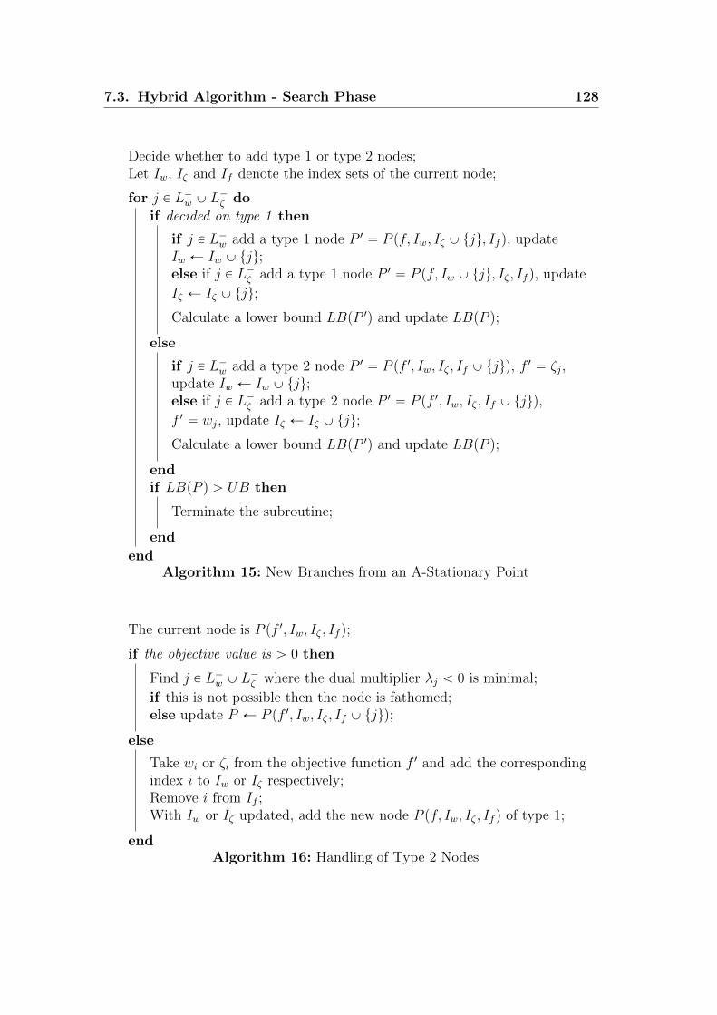
7.3. Hybrid Algorithm - Search Phase 128
Decide whether to add type 1 or type 2 nodes;Let Iw, Iζ and If denote the index sets of the current node;
for j P L´w Y L´ζ do
if decided on type 1 then
if j P L´w add a type 1 node P 1 “ P pf, Iw, Iζ Y tju, If q, updateIw Ð Iw Y tju;else if j P L´ζ add a type 1 node P 1 “ P pf, Iw Y tju, Iζ , If q, update
Iζ Ð Iζ Y tju;
Calculate a lower bound LBpP 1q and update LBpP q;
else
if j P L´w add a type 2 node P 1 “ P pf 1, Iw, Iζ , If Y tjuq, f1 “ ζj,
update Iw Ð Iw Y tju;else if j P L´ζ add a type 2 node P 1 “ P pf 1, Iw, Iζ , If Y tjuq,
f 1 “ wj, update Iζ Ð Iζ Y tju;
Calculate a lower bound LBpP 1q and update LBpP q;
endif LBpP q ą UB then
Terminate the subroutine;
end
endAlgorithm 15: New Branches from an A-Stationary Point
The current node is P pf 1, Iw, Iζ , If q;
if the objective value is ą 0 then
Find j P L´w Y L´ζ where the dual multiplier λj ă 0 is minimal;
if this is not possible then the node is fathomed;else update P Ð P pf 1, Iw, Iζ , If Y tjuq;
else
Take wi or ζi from the objective function f 1 and add the correspondingindex i to Iw or Iζ respectively;Remove i from If ;With Iw or Iζ updated, add the new node P pf, Iw, Iζ , If q of type 1;
endAlgorithm 16: Handling of Type 2 Nodes

7.3. Hybrid Algorithm - Search Phase 129
7.2 Theorem
If the CASET algorithm in algorithm 14 always terminates in a finite number of
steps, then algorithm 14 will find a global optimum for the MPEC (7.26) in a
finite number of steps if it exists.
Proof An overview of the algorithm is presented in the diagram of figure 7.6.
Assume that a global optimum for the MPEC (7.26) exists. Every leaf P “
P pf 1, Iw, Iζ , If q of the branch-and-bound tree meets one of the following situa-
tions:
• The lower bound LBpP q ě UB yields no further progress, thus the node
can be fathomed;
• The CASET algorithm has determined an A-stationary point of P and UB
has been updated. Then subroutine algorithm 15 creates new nodes as in
the BBASET algorithm (rem. 4.2);
• The CASET algorithm is unsuccessful and there is no complementarity
index that can be relaxed, i.e. Lw “ Lζ “ H. It follows that IwY Iζ Y If “
t1, . . . ,mu and the feasible set of the node problem (7.30) equals the set of
the relaxed problem (7.32) and both are empty.
In the type 2 nodes the algorithm releases complementarity indices by adding
them to If until the desired type 1 node is achieved or the infeasibility of this
branch is proven. Every type 2 node P pwj, Iw, Iζ , If q will eventually become a
type 1 node P pf, Iw Y tju, Iζ , I1f q, for some set I 1f , or determine that the later
is infeasible. And every type 2 node P pζj, Iw, Iζ , If q will eventually become a
type 1 node P pf, Iw, Iζ Y tju, I1f q, for some set I 1f , or determine that the later is
infeasible. The type 1 nodes, or their index sets Iw and Iζ , are the nodes that
are generated in the BBASET algorithm. Introducing type 2 nodes only delays
the investigation of the corresponding type 1 nodes, in order to find a feasible
constellation pLw, Lζ , If q for the CASET algorithm to start with.
It follows that algorithm 14 reproduces the branching structure of the BBASET
algorithm which finds a global optimum. �
Remark 7.4 Algorithm 14 can easily be modified to handle possibly unbounded
or infeasible problems. Assume a node P pf, Iw, Iζ , If q is found unbounded by
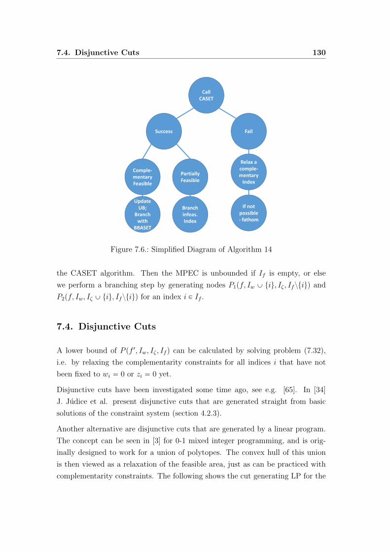
7.4. Disjunctive Cuts 130
Call
CASET
Success Fail
Comple-
mentary
Feasible
Partially
Feasible
Branch
infeas.
Index
Update
UB;
Branch
with
BBASET
Relax a
comple-
mentary
Index
If not
possible
- fathom
Figure 7.6.: Simplified Diagram of Algorithm 14
the CASET algorithm. Then the MPEC is unbounded if If is empty, or else
we perform a branching step by generating nodes P1pf, Iw Y tiu, Iζ , Ifztiuq and
P2pf, Iw, Iζ Y tiu, Ifztiuq for an index i P If .
7.4. Disjunctive Cuts
A lower bound of P pf 1, Iw, Iζ , If q can be calculated by solving problem (7.32),
i.e. by relaxing the complementarity constraints for all indices i that have not
been fixed to wi “ 0 or zi “ 0 yet.
Disjunctive cuts have been investigated some time ago, see e.g. [65]. In [34]
J. Judice et al. present disjunctive cuts that are generated straight from basic
solutions of the constraint system (section 4.2.3).
Another alternative are disjunctive cuts that are generated by a linear program.
The concept can be seen in [3] for 0-1 mixed integer programming, and is orig-
inally designed to work for a union of polytopes. The convex hull of this union
is then viewed as a relaxation of the feasible area, just as can be practiced with
complementarity constraints. The following shows the cut generating LP for the

7.4. Disjunctive Cuts 131
special case of positive complementary variables.
Let x be a feasible point of the relaxed program (7.32) where the i-th index
violates a complementarity constraint: wiζi ą 0. The cut generation LP is an
adaption of the cut generation LP in [3] and is of the form
maxuw,uζ ,vw,vζ
β ´ αT x
α ě CTuw ´ vwewi
α ě CTuζ ´ vζeζi
β ď uTwg
β ď uTζ g
´1 ď puwqj ď 1 @j “ 1, . . . , k
´1 ď puζqj ď 1 @j “ 1, . . . , k
(7.33)
where ewi and eζi denote the unit vectors corresponding to x “ py, w, ζq, where
the pdimpyq` iq-th or the pdimpyq`m` iq-th component are 1 respectively. The
system contains decision variables uw, uζ , vw and vζ . We note that vw and vζ
may be eliminated along with the corresponding constraints in which they are
used.
If the objective value of pα, βq in (7.33) is greater than zero we receive a cut
αTx ě β that excludes x. The bounds on uw and uζ restrict the feasible cone to
a polytope. These constraints have been suggested in the original article [3] to
avoid unbounded solutions.
7.3 Lemma
The generated cuts of (7.33) are globally valid for the MPEC (7.26).
Proof Let pα, βq be a cut generated from 7.33. Let us assume that x “ py, w, ζq
is feasible for the system in the MPEC (7.26). Thus it holds that wi “ 0 or ζi “ 0
for i “ 1, . . . ,m. We conclude that either
αTx ě pCTuwqTx´ pvwewiq
Tx “ uTwg ě β, (7.34)

7.5. Constraints based on the Objective Function Gradient 132
is satisfied or else it holds that
αTx ě pCTuζqTx´ pvζeζiq
Tx “ uTζ g ě β. (7.35)
�
The authors also emphasize the importance of cut strengthening. For further
information we refer the reader to the original article [3].
7.5. Constraints based on the Objective Function
Gradient
The convexity of the objective function allows the possibilty to use its lineariza-
tion at a given point as lower bound in the solution process. In the search phase
of the hybrid algorithm, these linearizations are used in the form of additional
constraints.
For a given point x0 “ py, w, ζq it holds that
@x : fpxq ě ∇fpx0qTpx´ x0q ` fpx0q. (7.36)
Assuming we are only interested in points x with an objective value fpxq ď UB,
it holds that
UB ě fpxq ě ∇fpx0qTpx´ x0q ` fpx0q (7.37)
which leads to the constraint
∇fpx0qTx ď ∇fpx0q
Tx0 ` UB ´ fpx0q. (7.38)
Some of the investigated branches of the binary search tree may be identified
as infeasible after the application of such constraints. The more common case,
however, is that the branch is not completely infeasible, but initialization of the
CASET algorithm on this branch fails. The working sets Lw and Lζ are part of
this problem, since they are not updated with the introduction of new constraints.

7.6. Hybrid Algorithm - Global Optimality 133
In order to confirm the infeasibility of the node (which is frequently the case in
practice) we need to solve a general linear complementarity problem, which by
itself is still NP-hard (see e.g. [30]).
In the search phase, an investment of too many resources for a complete search
that investigates every branch is not desired. It is preferred to explore many
solutions that are easily accessible. In the current implementation a priority
system is used which marks individual nodes with a number that supposedly
indicates whether they are more or less promising to solve. Nodes where the
CASET algorithm fails in its first iteration receive a low priority value, and can
be postponed until further investigation.
We note that these constraints can greatly compromise the numerical stability
and speed of a convex solver depending on the given constraint system of the
MPEC. They can also lead to a larger branch-and-bound tree. In the related
experiments they have only been used in few iterations of the search phase.
7.6. Hybrid Algorithm - Global Optimality
The second phase of the hybrid algorithm focuses on the proof of global opti-
mality. Experiments have shown that application of the search phase tends to
create a large number of nodes in a short time. The second phase avoids this by
focusing on the lower bounds when it comes to expansion of the search tree.
7.6.1. Branching Strategies
The selection of the branching variable in integer programs, or branching index
for complementarity constraints, naturally has a large impact on the size of the
search tree, and therefore on the performance of a branch-and-bound algorithm.
Selecting the index with the largest feasibility violation from the solution of the
relaxed problem is just one of them. Many techniques have already been estab-
lished for different types of mixed integer programs, see e.g. [6].
Notation: Let Ic be the candidate set of all branching variables.
We review some of the branching strategies for integer programs in brief:

7.6. Hybrid Algorithm - Global Optimality 134
• Selecting
argmaxiPIctminpxi ´ txiu, rxis´ xiqu (7.39)
is called most fractional branching.
• Strong branching computes lower bounds for all choices in Ic. The increase
in the lower bound (on a minimization problem) is monitored for each
variable in order to pick the one with the largest increase.
• Pseudocost branching tries to estimate the lower bound increase by logging
the effects of past decisions and estimating the current one.
A look at the website of the Gurobi optimizer [71] suggests that possible technical
details in branch-and-bound algorithms are of arbitrary complexity:
In addition (. . . ), a modern MIP solver will include a long list of
additional techniques. A few examples include sophisticated branch
variable selection techniques, node presolve, symmetry detection, and
disjoint subtree detection. The goal in most cases is to limit the size
of the branch-and-bound tree that must be explored.
Another aspect of a branch-and-bound algorithm is the selection of the next node
to process. Different strategies are possible and three of the main principles are
• Depth first - selecting a deepest live node in the branch-and-bound tree.
The depth of a node increases with every branching choice that has been
made.
• Best first - selecting a node that has a minimal lower bound (in a mini-
mization problem).
• Breadth first - the nodes of the current depth-level in the search tree are
explored before advancing to the next level.
The depth first strategy is often used to generate an upper bound early in the
process. The best bound strategy can effectively be used to prove the optimality
of a given solution. So called diving strategies can be used as a combination of
different concepts where qualities are utilized as needed. For more details on this
topic see e.g. [56].

7.6. Hybrid Algorithm - Global Optimality 135
For further considerations if not stated differently, we assume that the depth first
strategy is chosen for the selection of the next node.
Most Infeasible Branching
For the sake of completeness, the algorithm that solves a program with linear
complementarity constraints by most infeasible branching is stated in application
to a node problem P pf, I0w, I
0ζ , I
0f q. The result is algorithm 17.
The algorithm returns with a globally optimal solution of P pf, I0w, I
0ζ , I
0f q with
respect to a feasibility tolerance of εFEAS and tolerance on the objective value of
εGAP if one exists. Otherwise it returns with an upper bound UB “ 8.
Other Branching Strategies
In [46] an idea for MIQP branching by Korner investigates the cardinality of the
projection of level sets onto a potential branching variable.
Let a problem with quasiconvex objective function (def. 2.13) be given by
min fpxq
x PM “ tx P Rn| gjpxq ď 0, j “ 1, . . . ,mu
xi P Z
(7.40)
where f is quasiconvex and M convex. Let the level set be
M˚“ tx| fpxq ď UB, x PMu (7.41)
for a given upper bound UB. Let Mi be the projection of M˚ onto the axis xi. In
[46] Korner states that under relatively simple assumptions, one can show that
the search tree consists of a minimal number of nodes if the variable xj with the
following properties is branched:
cardpMj X Zq ď cardpMi X Zq, @i P Ic. (7.42)
We explain the approach that is used to prove this statement: Let x1 be the
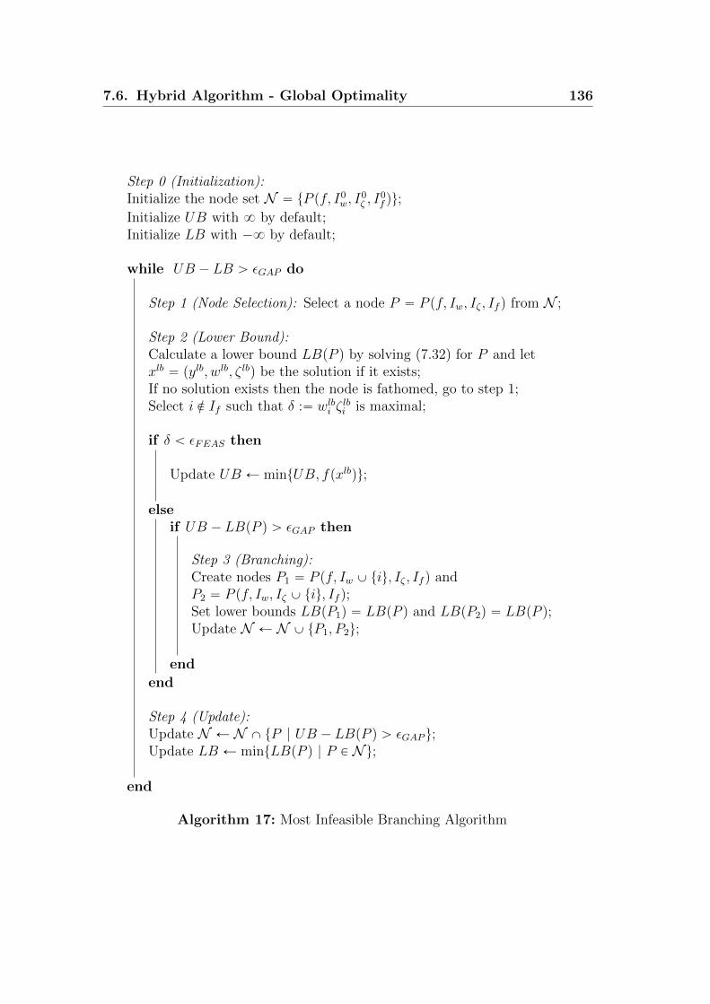
7.6. Hybrid Algorithm - Global Optimality 136
Step 0 (Initialization):Initialize the node set N “ tP pf, I0
w, I0ζ , I
0f qu;
Initialize UB with 8 by default;Initialize LB with ´8 by default;
while UB ´ LB ą εGAP do
Step 1 (Node Selection): Select a node P “ P pf, Iw, Iζ , If q from N ;
Step 2 (Lower Bound):Calculate a lower bound LBpP q by solving (7.32) for P and letxlb “ pylb, wlb, ζ lbq be the solution if it exists;If no solution exists then the node is fathomed, go to step 1;Select i R If such that δ :“ wlbi ζ
lbi is maximal;
if δ ă εFEAS then
Update UB Ð mintUB, fpxlbqu;
elseif UB ´ LBpP q ą εGAP then
Step 3 (Branching):Create nodes P1 “ P pf, Iw Y tiu, Iζ , If q andP2 “ P pf, Iw, Iζ Y tiu, If q;Set lower bounds LBpP1q “ LBpP q and LBpP2q “ LBpP q;Update N Ð N Y tP1, P2u;
end
end
Step 4 (Update):Update N Ð N X tP | UB ´ LBpP q ą εGAP u;Update LB Ð mintLBpP q | P P N u;
end
Algorithm 17: Most Infeasible Branching Algorithm

7.6. Hybrid Algorithm - Global Optimality 137
solution of the relaxed problem at the current node. Korner’s branching step of
a variable xi is performed by generating new nodes for every value
rx1is ´ k´, . . . , rx1is ` k
` (7.43)
where k´ is the largest value of k, such that the current node with additional
constraint xi “ rx1is´k
´ is either infeasible or has a larger lower bound than UB
(and can therefore be pruned). The value k` is defined analogously.
7.4 Lemma ([45] Lem. 1)
If a node is selected by the best first strategy, and criterion (7.42) is satisfied for
j, then the number of nodes generated by branching j directly before i is less
than or equal to the number of nodes created by branching i directly before j
(for every i P Ic).
Proof The proof in [45] is rather short, and focuses on the fact that after branch-
ing twice both alternatives have branched xi and xj (although in different order).
Since the branching step generates every feasible node with valid objective value,
the number of generated nodes with children is equal to the number cardpMjXZqor cardpMi X Zq respectively. These are the numbers of property (7.42). �
Checking property (7.42) is most likely to be very impractical for a branch-and-
bound solver in many instances. To overcome this difficulty the diameter of these
sets is evaluated instead, which is defined by
dpMiq “ supt}x´ y} | x, y PMiu. (7.44)
It is suggested to branch the variable with minimal diameter. Formulas on how
to evaluate or approximate this value are carried out especially for the case of
quadratic integer programs. For more details see [46, 44, 43].
These techniques inspire a procedure for problems with complementarity con-
straints. If a complementarity constraint wiζi “ 0 is modeled with an integer
variable xi (see chapter 5) then the following relation holds
cardpMi X Zq “ cardpM˚X twi “ 0, ζi ě 0uq ` cardpM˚
X twi ě 0, ζi “ 0uq.
(7.45)

7.6. Hybrid Algorithm - Global Optimality 138
This means that cardpMi X Zq just holds the information - whether both com-
plementary affine linear sets are a non-negligible part of the level set M˚ or not.
The diameter of the level set, on the other hand, might be richer in information.
We continue with the following idea:
Let wiζi “ 0 (i “ 1, . . . ,m) be the complementarity constraints as before. For ev-
ery index i we maximize wi under the restriction ζi “ 0 and analogously maximize
ζi under wi “ 0 on the set M˚. The result are values wmaxi , ζmaxi :
wmaxi :“ maxwi
px,w, ζq PM˚(7.46)
ζmaxi :“ max ζi
px,w, ζq PM˚(7.47)
These values can be used to
• either to eliminate a branching candidate if one of them is zero,
• or to introduce a new constraint on this pair of variables:
wiζmaxi ` ζiw
maxi ď wmaxi ζmaxi . (7.48)
The values wmaxi and ζmaxi can be8 if wi or ζi respectively are unbounded on M˚.
In this case the constraint (7.48) can be reduced to variable bounds wi ď wmaxi
if ζmaxi “ 8 and ζi ď ζmaxi if wmaxi “ 8.
This type of constraints has also been investigated in other algorithms for prob-
lems with complementarity constraints. E.g. in [55] where Mitchell et al. present
a so called bound tightening procedure. Furthermore one could use the values
ζmaxi and wmaxi as a source of information for a heuristic on the selection of the
next branching index in the branch-and-bound algorithm.
7.6.2. Application to the Reweighting Bilevel Problem
A subroutine has been developed for the MPEC of the reweighting bilevel problem
(section 3.4.1) that generates the constraints of the type in (7.48). The principle
can be adapted for other affine linear complementarity constraints, but might not
be as useful if the auxiliary problems (7.46) and (7.47) are unbounded. In this
case little information is gained from the subroutine.

7.6. Hybrid Algorithm - Global Optimality 139
A formulation of the reweighting bilevel MPEC shall be restated here (def. 3.8),
the subscript λ on T , A, t and b is left out for the sake of legibility):
minλ,w,ζ
}Tλ´ t}2
b´ Aλ´ w1` w2
“ 0
λ` ζ1ě λmin
λ´ ζ2ď ´λmin
´λmaxe ď λ ď λmaxe
0 ď w “ pw1, w2q K ζ “ pζ1, ζ2
q ě 0.
(7.49)
Let λ˚i for i P Is be a set of feasible points that have been found in the overall
branch-and-bound algorithm. We state the level set for the subroutine as
M˚“ tλ| }Tλ´ t}2 ď }Tλ˚i ´ t}
2, @i P Isu. (7.50)
We approximate the level set with a number of linear constraints. Let ∆iλ “ λ˚i ´ λ
and Q “ T TT and let UB be the current upper bound. The constraint is derived
by a Taylor approximation
UB ě }Tλ´ t}2 “ ∆iλTQ∆iλ´ 2λ˚Ti Q∆iλ` λ
˚Ti Qλ˚i ` t
TTλ` tT t
ě ´2λ˚Ti Q∆iλ` λ˚Ti Qλ˚i ` t
TTλ` tT t.(7.51)
Another set of constraints can be derived by a projection onto the vectors fi
which shall be defined as
fi “Tλ˚i ´ t
}Tλ˚i ´ t}. (7.52)
Let πfi be the projection on the linear subspace that is generated by the vector
fi. It holds that
}Tλ´ t}2 ě }πfipTλ´ tq}2
“ }fTi pTλ´ tq}2.
(7.53)
With the current (positive) upper bound we receive two linear constraints for
every index i P Is:

7.6. Hybrid Algorithm - Global Optimality 140
´?UB ď fTi pTλ´ tq ď
?UB (7.54)
The number of feasible points λ˚i which is used to generate these constraints
determines how many of them are present in the bound generation LPs (7.46) and
(7.47). By intuition we suggest to limit their number, and secondly to include the
incumbent feasible solution. This has been practiced in the related experiments.
The collection of the aforementioned constraints (7.51) and (7.54) with the non-
complementarity constraints of system (7.49) defines an approximation for the
level set M˚ that shall be denoted by M . The subroutine that describes the
generation of the variable bounds and constraints is algorithm 18.
Preliminaries for Algorithm 18
Assume that λlb is the solution of the lower bound problem for the current node.
Furthermore let I1c , I
2c Ď t1, . . . ,mu be the candidates of branching indices i,
where branching on i P I1c is associated with introducing two nodes for the con-
straints w1 “ 0 and ζ1 “ 0 respectively. The indices in I2c are related analogously.
The complementary affine linear expressions are noted as
wipλq :“ pb´ Aλqi
ζ1i pλq :“ λmin ´ λi
ζ2i pλq :“ λ` λmin.
(7.55)
A heuristic order on the sets I1c and I2
c is used that sorts the indices by their
magnitude of complementary infeasibility defined by the products
maxt0, wipλqumaxt0, ζ1i pλqu, i P I
1c
maxt0,´wipλqumaxt0, ζ2i pλqu, i P I
2c .
(7.56)
We note the following relations for feasible points pλ,w, ζq of the MPEC (7.49)
that are used within the algorithm:

7.6. Hybrid Algorithm - Global Optimality 141
wipλq ă 0 ñ pb´ Aλqi ă 0 ñ w2i ą 0 ñ ζ2
i “ 0
wipλq ą 0 ñ pb´ Aλqi ą 0 ñ w1i ą 0 ñ ζ1
i “ 0
ζ1i pλq ă 2λmin ñ λ ą ´λmin ñ ζ2
i ą 0 ñ w2i “ 0
ζ2i pλq ă 2λmin ñ λ ă λmin ñ ζ1
i ą 0 ñ w1i “ 0.
(7.57)
We also introduce update lists pLα,βwwqi, pLα,βwζ qi, pL
α,βζw qi and pLα,βζζ qi for α, β “ 1, 2
and i “ 1, . . . ,m. The update lists record the indices of the other affine linear
complementary expressions that are positive at the corresponding LP solutions.
Their definition can be seen within algorithm 18. In practice we use the following
strategy. A node problem for the reweighting bilevel MPEC is given by
minλ,w,ζ
}Tλ´ t}2
b´ Aλ´ w1` w2
“ 0
λ` ζ1ě λmin
λ´ ζ2ď ´λmin
´λmaxe ď λ ď λmaxe
w1i “ 0, @i P I1
w
w2i “ 0, @i P I2
w
ζ1i “ 0, @i P I1
w
ζ2i “ 0, @i P I2
w
w1i ζ
1i “ 0, @i P I1
f
w2i ζ
2i “ 0, @i P I2
f
(7.58)
for index sets I1w, I
2w, I
1ζ , I
2ζ , I
1f , I
2f . Let Λ denote the points that are feasible in the
constraint set of (7.58) but without the complementarity constraints. It follows
that Λ is convex.
For child nodes only those bounds wmaxi and ζmaxi of branching candidates will
be updated where the following situations apply:
if k has entered I1w then every index i P I1
c where k P pL11wwqi or k P pL11
ζwqi and
every index i P I2c where k P pL21
wwqi or k P pL21ζwqi will be updated;
if k has entered I2w then every index i P I1
c where k P pL12wwqi or k P pL12
ζwqi and

7.6. Hybrid Algorithm - Global Optimality 142
every index i P I2c where k P pL22
wwqi or k P pL22ζwqi will be updated;
if k has entered I1ζ then every index i P I1
c where k P pL11wζqi or k P pL11
ζζqi and
every index i P I2c where k P pL21
wζqi or k P pL21ζζqi will be updated;
if k has entered I2ζ then every index i P I1
c where k P pL12wζqi or k P pL12
ζζqi and
every index i P I2c where k P pL22
wζqi or k P pL22ζζqi will be updated.
For all other indices the old values and update lists will be reused. With this
update strategy it is possible to save a considerate amount of LP solve calls.
Algorithm 18 shows the procedure for every index in I1c and I2
c .
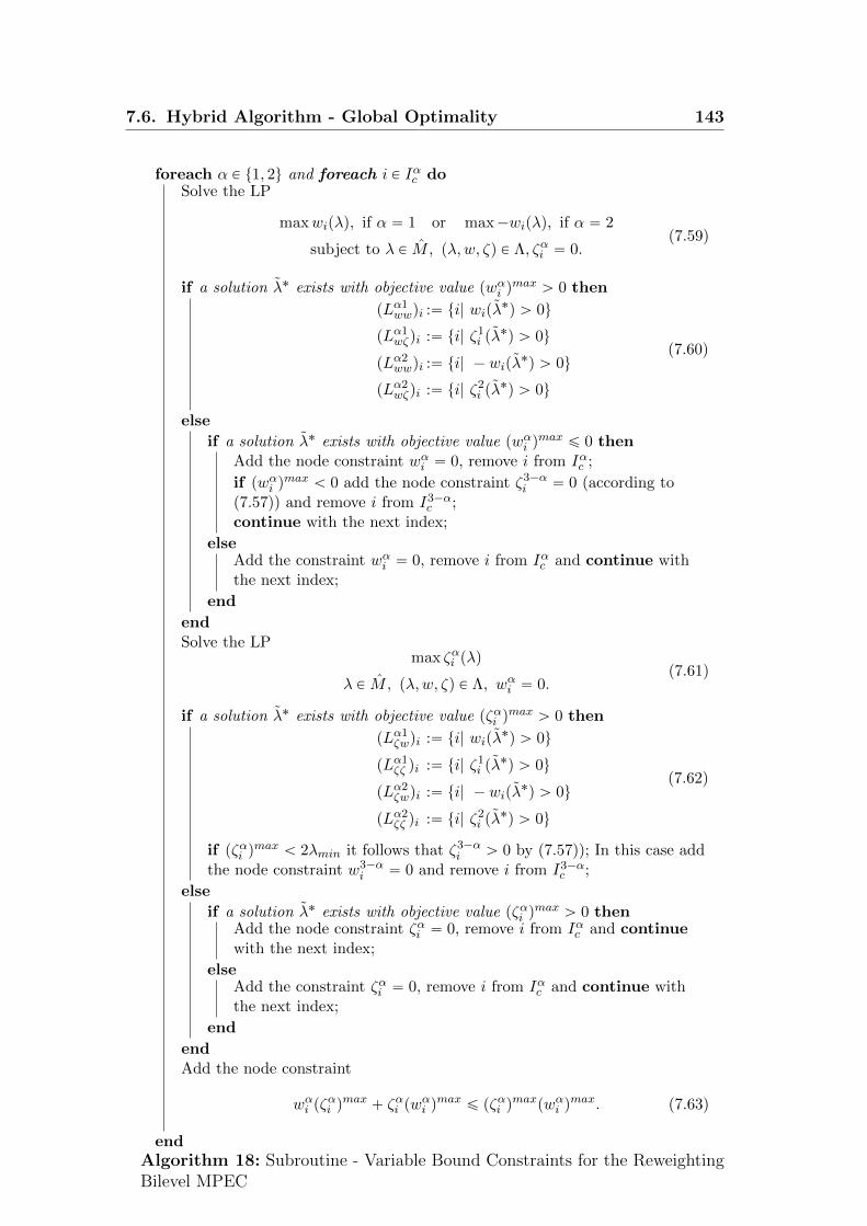
7.6. Hybrid Algorithm - Global Optimality 143
foreach α P t1, 2u and foreach i P Iαc doSolve the LP
maxwipλq, if α “ 1 or max´wipλq, if α “ 2
subject to λ P M, pλ,w, ζq P Λ, ζαi “ 0.(7.59)
if a solution λ˚ exists with objective value pwαi qmax ą 0 then
pLα1wwqi :“ ti| wipλ
˚q ą 0u
pLα1wζqi :“ ti| ζ1
i pλ˚q ą 0u
pLα2wwqi :“ ti| ´ wipλ
˚q ą 0u
pLα2wζqi :“ ti| ζ2
i pλ˚q ą 0u
(7.60)
else
if a solution λ˚ exists with objective value pwαi qmax ď 0 then
Add the node constraint wαi “ 0, remove i from Iαc ;
if pwαi qmax ă 0 add the node constraint ζ3´α
i “ 0 (according to(7.57)) and remove i from I3´α
c ;continue with the next index;
elseAdd the constraint wαi “ 0, remove i from Iαc and continue withthe next index;
end
endSolve the LP
max ζαi pλq
λ P M, pλ,w, ζq P Λ, wαi “ 0.(7.61)
if a solution λ˚ exists with objective value pζαi qmax ą 0 then
pLα1ζwqi :“ ti| wipλ
˚q ą 0u
pLα1ζζ qi :“ ti| ζ1
i pλ˚q ą 0u
pLα2ζwqi :“ ti| ´ wipλ
˚q ą 0u
pLα2ζζ qi :“ ti| ζ2
i pλ˚q ą 0u
(7.62)
if pζαi qmax ă 2λmin it follows that ζ3´α
i ą 0 by (7.57)); In this case addthe node constraint w3´α
i “ 0 and remove i from I3´αc ;
else
if a solution λ˚ exists with objective value pζαi qmax ą 0 then
Add the node constraint ζαi “ 0, remove i from Iαc and continuewith the next index;
elseAdd the constraint ζαi “ 0, remove i from Iαc and continue withthe next index;
end
endAdd the node constraint
wαi pζαi qmax ` ζαi pw
αi qmax ď pζαi q
maxpwαi qmax. (7.63)
endAlgorithm 18: Subroutine - Variable Bound Constraints for the ReweightingBilevel MPEC

7.6. Hybrid Algorithm - Global Optimality 144
7.6.3. A Modification of the BBASET Method
The BBASET method generates a number of new nodes from a complementarity
feasible strongly stationary point. The indices are ordered by the negativity of
their dual multiplier, with preference to the most negative value. An interpreta-
tion of this approach is that BBASET prefers to explore nodes in the binary search
tree that look most promising when it comes to lowering the upper bound. Com-
putational experience within the extent of this work has shown that BBASET
performs well in finding many different local solutions with low objective value.
However, this does not have to be beneficial in terms of increasing the current
lower bound of the program.
In the second phase of the hybrid algorithm a modification of the BBASET
scheme is performed which originates from two key points:
1) For any feasible point x0 P Rn we can use the linearization of f
flinpxq “ ∇fpx0qTpx´ x0q ` fpx0q (7.64)
as a lower bound for f since f is convex. Note that f was defined to be any
differentiable convex function. In the application, this approach is mainly used
in situations where the number of nodes created from one stationary point is
very large. Calculating lower bounds for each of them can be costly, and may be
cheaper if a linear function is used.
2) The second point is that one can store the product wlbi ζlbi when calculating a
lower bound. With this information, it is possible to generate new nodes by a
hybrid behavior that combines BBASET and most infeasible branching. This is
achieved by ordering the indices not by the magnitude of their dual multipliers,
but by the product wlbi ζlbi beginning with the greatest.
7.6.4. The Method of Hu et al. and Lagrange Lower Bounds
In section 7.6.5 the hybrid algorithm in search for global optimality will be stated.
The following presents a list of the modules that are incorporated.

7.6. Hybrid Algorithm - Global Optimality 145
Subroutine - Feasibility Module
The algorithm of Hu et al. [24] and an adaption were presented in chapter 5.
The adapted algorithm (sec. 5.3.1) is now embedded in the branch-and-bound
algorithm for the MPEC (7.26). For a node Problem P “ P pf, Iw, Iζ , If q the
remaining complementarity working indices are
Lw Y Lζ “ t1, . . . ,muzIwzIζzIf . (7.65)
The adapted method finds disjunct sets L1w, L1ζ and I 1f such that P pf, Iw, Iζ , I1f q
with the working sets L1w and L1ζ provides a suitable entry point for the CASET
algorithm, i.e. P pf, Iw Y L1w, Iζ Y L
1ζ , I
1f q is feasible.
If I 1f is nonempty then integer sets for a partially feasible solution (def. 5.4) have
been generated.
Elements of the set t0, 1um are associated with the leaves of the branch-and-
bound tree. The leaves of a node problem P with index sets Iw and Iζ are given
by
Pz “ tz P t0, 1um|zi “ 0 if i P Iw, zi “ 1 if i P Iζu. (7.66)
The method keeps track of a feasible set Zwork Ď t0, 1um. The set Zwork contains
the cuts on t0, 1um that imply this feasible set. They are generated during the
process and prune branches of the binary tree.
An efficient management of the working set Zwork is needed to evaluate as much
information from the surrounding algorithm as possible. For instance, if the
CASET subroutine solves a convex program and the objective function value
is greater than the current upper bound, then it would be completely correct
(meaning without compromising the enumeration of the search tree) to introduce
a binary constraint that prunes this part of the feasible set Zwork. However,
depending on the number of relaxed indices If in the CASET subroutine, this
simple cut might turn out to be very dense. A MIP solver or SAT solver that
operates on the set can be slowed significantly by such cuts, which provide only
little information. Thus it might be important to find a good management system
for the set Zwork.

7.6. Hybrid Algorithm - Global Optimality 146
Considering the method of cut sparsification (sec. 5.2.2) we note that this pro-
cedure generates lower bounds from the information at the bottom of the tree
(near the leaves) and tries to carry this information further to the top (near the
root). The hybrid branch-and-bound algorithm will start with the primal system
from the top of the tree, and tries to prune branches by calculating lower bounds
as soon as possible. The method of cut sparsification seems not very efficient in
this context, since it works in reverse direction. Sparsifying a cut requires the
solution of relaxed node programs, and is therefore considered resource demand-
ing. Computational experiments have confirmed this assumption for the given
instances.
Lagrange Lower Bounds
Chapter 6 presented how the Lagrange function can be used to calculate lower
bounds in a problem with linear complementarity constraints. For a given vector
λ we state the program that needs to be solved in order to find such a bound for
the node problem P pf, Iw, Iζ , If q using the representation of the tree with binary
vectors z P Zwork:
minx,z
flagrpxq :“ fpxq ` λpg ´ Cxq
z P Zwork X Pzwi “ 0 if zi “ 0
ζi “ 0 if zi “ 1
x “ py, w, ζq ě 0.
(7.67)
As mentioned in section 6.3, this convex program with positive complementary
variable constraints can be solved by the BBASET algorithm, without the issue
of finding feasible startpoints.
If the solution process of system (7.67) works with a branch-and-bound algorithm
itself (e.g. BBASET), then branches of this algorithm can be identified with the
branches of the surrounding algorithm. Every branch where an objective value
of flagr is detected, that is greater than or equal to the current upper bound in
the surrounding algorithm, can be pruned in both search trees.

7.6. Hybrid Algorithm - Global Optimality 147
7.6.5. The Hybrid Algorithm
We initialize every node P with a lower bound LBpP q, which is the lower bound
of the parent node or ´8 for the root node. The global lower bound LB is
automatically updated to the minimal lower bound of all remaining nodes. Nodes
with a lower bound LB ě UB greater than the current upper bound UB are
removed from the node set N . The working sets Lw and Lζ are inherited from
the parent node, and are updated in order to stay well defined, i.e. they have no
intersection with Iw, Iζ or If .
7.3 Theorem
If the convex problems in the hybrid algorithm 19 are solved in a finite number
of steps, and every feasible node problem is bounded, then the hybrid algorithm
finds a global optimum of the MPEC (7.26) in a finite number of steps if it exists.
Proof Every node receives a lower bound in the first part of the algorithm. In
the second part the node is either processed by the BBASET subroutine in step 5,
or a branching index is selected in step 6 where two new child nodes are created.
First we show that the branching behavior in step 5 is correct.
On the Correctness of Step 5b
The modification from section 7.6.3 creates the same branches as the BBASET
algorithm (see remark 4.2) just in different order. We have to show that the
relaxed complementarity constraints with corresponding indices in If do not affect
the enumeration of the search tree.
Let x˚ be an A-stationary point of P pIw, Iζ , If q with working sets Lw and Lζ and
objective value fpx˚q ě UB. The point x˚ is the optimal solution of the convex
problem
minxě0
fpxq
Cx “ g
wi “ 0, @i P Iw Y Lw
ζi “ 0, @i P Iζ Y Lζ
(7.68)

7.6. Hybrid Algorithm - Global Optimality 148
Initialize the set Zwork “ t0, 1um;Initialize the set of nodes with N “ tP pf,H,H,Hq };Initialize disjunct working sets Lw, Lζ Ď t1, . . . ,mu;Initialize UB “ 8 and LB “ ´8;
Step 0 (Termination): If UB ´ LB ď 0 terminate;
Step 1a (Node Selection): Select the current node P from N such thatLBpP q ă UB;Update N Ð N ztP u;
Step 1b (Node Check): If Pz X Zwork “ H go to step 0 (the node isfathomed);
Step 2a (Lower Bound): Calculate a lower bound LBpP q by solving(7.32) and let xlb “ pylb, wlb, ζ lbq be the solution if it exists; If not then Pis infeasible - go to step 0;
Step 2b (Lower Bound): Decide whether to calculate a Lagrange lowerbound by solving (7.67);Update LBpP q and Zwork accordingly;
if LBpP q ă UB thenif miniw
lbi ζ
lbi ą 0 then
Step 3 (Disjunctive Cut): Possibly add a disjunctive cut by solving(7.33);If a cut was added go to Step 2a;
else
xlb is feasible: Update UB Ð mintUB, fpxlbqu;Update N Ð N X tP | LBpP q ă UBu;
end
elseGo to step 0 (the node is fathomed);
endAlgorithm 19: Hybrid Algorithm - Phase 2 - Part 1
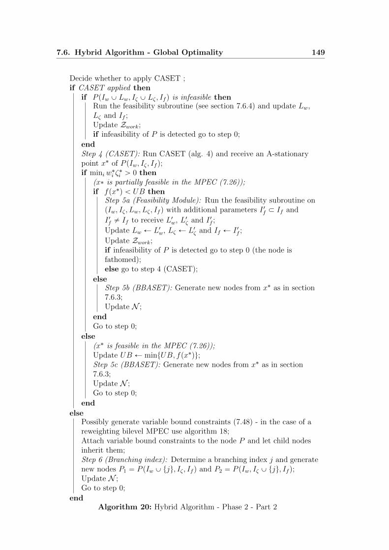
7.6. Hybrid Algorithm - Global Optimality 149
Decide whether to apply CASET ;if CASET applied then
if P pIw Y Lw, Iζ Y Lζ , If q is infeasible thenRun the feasibility subroutine (see section 7.6.4) and update Lw,Lζ and If ;Update Zwork;if infeasibility of P is detected go to step 0;
endStep 4 (CASET): Run CASET (alg. 4) and receive an A-stationarypoint x˚ of P pIw, Iζ , If q;if miniw
˚i ζ˚i ą 0 then
(x˚ is partially feasible in the MPEC (7.26));if fpx˚q ă UB then
Step 5a (Feasibility Module): Run the feasibility subroutine onpIw, Iζ , Lw, Lζ , If q with additional parameters I 1f Ă If and
I 1f ‰ If to receive L1w, L1ζ and I 1f ;
Update Lw Ð L1w, Lζ Ð L1ζ and If Ð I 1f ;
Update Zwork;if infeasibility of P is detected go to step 0 (the node isfathomed);else go to step 4 (CASET);
elseStep 5b (BBASET): Generate new nodes from x˚ as in section7.6.3;Update N ;
endGo to step 0;
else(x˚ is feasible in the MPEC (7.26));Update UB Ð mintUB, fpx˚qu;Step 5c (BBASET): Generate new nodes from x˚ as in section7.6.3;Update N ;Go to step 0;
end
elsePossibly generate variable bound constraints (7.48) - in the case of areweighting bilevel MPEC use algorithm 18;Attach variable bound constraints to the node P and let child nodesinherit them;Step 6 (Branching index): Determine a branching index j and generatenew nodes P1 “ P pIw Y tju, Iζ , If q and P2 “ P pIw, Iζ Y tju, If q;Update N ;Go to step 0;
endAlgorithm 20: Hybrid Algorithm - Phase 2 - Part 2

7.6. Hybrid Algorithm - Global Optimality 150
Let x˚ be the solution of the following problem:
minxě0
fpxq
Cx “ g
wi “ 0, @i P Iw Y Lw
ζi “ 0, @i P Iζ Y Lζ
wiζi “ 0, @i P If .
(7.69)
Then x˚ is an A-stationary point of the MPEC (7.26) (by thm. 4.5). We recall
that
If “ t1, . . . ,muzpIw Y Lw Y Iζ Y Lζq. (7.70)
It follows that
UB ď fpx˚q ď fpx˚q. (7.71)
The full evaluation of the branch pIw, Iζq in the search tree is the solution of
P pIw, Iζ ,Hq. (7.72)
Let ti1w, . . . , ilww u and ti1ζ , . . . , i
lζζ u be the index sets of the corresponding negative
dual multipliers λiw or λiζ at x˚. We define a cascade of index sets just in the
same manner as for the BBASET algorithm:
J1 :“ pIw Y ti1ζu, Iζ ,Hq
J2 :“ pIw Y ti2ζu, Iζ Y ti
1ζu,Hq
J3 :“ pIw Y ti3ζu, Iζ Y ti
1ζ , i
2ζu,Hq
. . .
Jlζ :“ pIw Y tilζζ u, Iζ Y ti
1ζ , . . . , i
lζ´1
ζ u,Hq
Jlζ`1 :“ pIw, Iζ Y ti1ζ , . . . , i
lζζ , i
1wu,Hq
Jlζ`2 :“ pIw Y ti1wu, Iζ Y ti
1ζ , . . . , i
lζζ , i
2wu,Hq
. . .
Jlζ`lw :“ pIw Y ti1w, . . . , i
lww u, Iζ Y ti
1ζ , . . . , i
lζζ u,Hq
(7.73)
It holds that
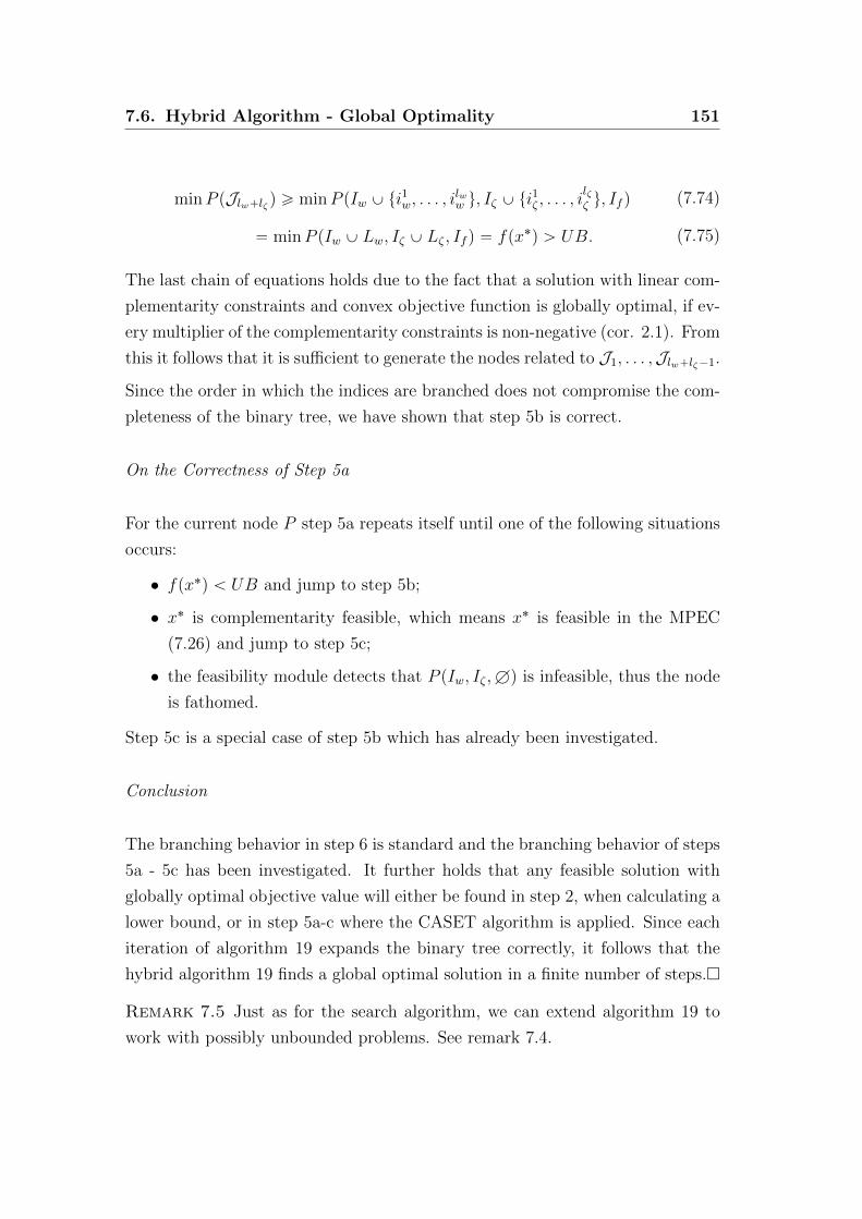
7.6. Hybrid Algorithm - Global Optimality 151
minP pJlw`lζq ě minP pIw Y ti1w, . . . , i
lww u, Iζ Y ti
1ζ , . . . , i
lζζ u, If q (7.74)
“ minP pIw Y Lw, Iζ Y Lζ , If q “ fpx˚q ą UB. (7.75)
The last chain of equations holds due to the fact that a solution with linear com-
plementarity constraints and convex objective function is globally optimal, if ev-
ery multiplier of the complementarity constraints is non-negative (cor. 2.1). From
this it follows that it is sufficient to generate the nodes related to J1, . . . ,Jlw`lζ´1.
Since the order in which the indices are branched does not compromise the com-
pleteness of the binary tree, we have shown that step 5b is correct.
On the Correctness of Step 5a
For the current node P step 5a repeats itself until one of the following situations
occurs:
• fpx˚q ă UB and jump to step 5b;
• x˚ is complementarity feasible, which means x˚ is feasible in the MPEC
(7.26) and jump to step 5c;
• the feasibility module detects that P pIw, Iζ ,Hq is infeasible, thus the node
is fathomed.
Step 5c is a special case of step 5b which has already been investigated.
Conclusion
The branching behavior in step 6 is standard and the branching behavior of steps
5a - 5c has been investigated. It further holds that any feasible solution with
globally optimal objective value will either be found in step 2, when calculating a
lower bound, or in step 5a-c where the CASET algorithm is applied. Since each
iteration of algorithm 19 expands the binary tree correctly, it follows that the
hybrid algorithm 19 finds a global optimal solution in a finite number of steps.�
Remark 7.5 Just as for the search algorithm, we can extend algorithm 19 to
work with possibly unbounded problems. See remark 7.4.

8. Computational Results
Rounding off the theoretical concepts of chapter 7, a test implementation has been
created. Although the methods are mostly designed for problems with convex
objective functions (and linear complementarity constraints) in general, the tests
have been performed on instances that limit to quadratic objective functions. The
foundation is a branch-and-bound framework in the language C# that manages
a variety of components.
8.1. Components
Core Solver
The main component is denoted the core solver, which is based around an ad-
justable Cplex model. For each pair of complementary variables 0 ď wiKzi ě 0
the solver includes one of the following pairs of constraints
• wi ě 0 “ zi
• zi ě 0 “ wi
• wi, zi ě 0
and thereby solves a convex problem, that is tightened in some of the complemen-
tary indices, and relaxed in the rest of them. In addition to this, the objective
function can be exchanged for linear expressions, such as the minimization of zi
or wi, for any of the complementary pairs of variables pwi, ziq. This is used in
accordance with section 7.3.1 and connected with the generation of type 2 nodes.
Another application of linear objective functions is the generation of the variable
bound constraints in accordance to section 7.6.2.
The core solver also accepts the introduction and removal of additional constraints
in the subroutines as needed.
152
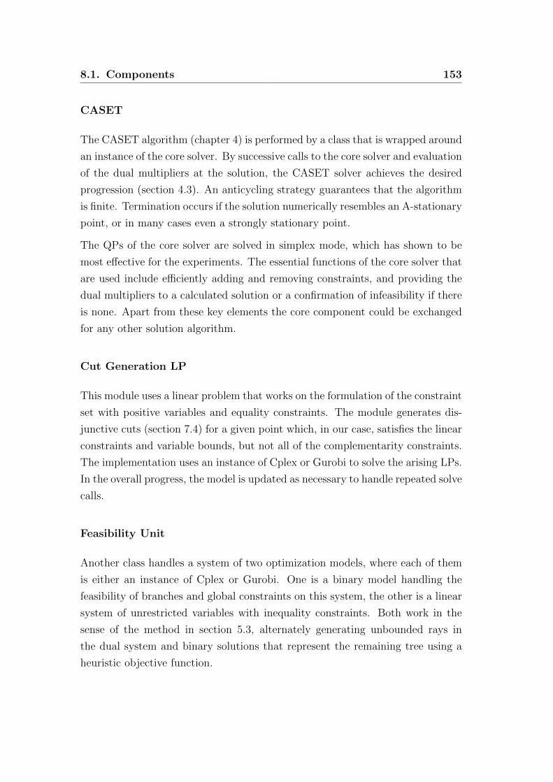
8.1. Components 153
CASET
The CASET algorithm (chapter 4) is performed by a class that is wrapped around
an instance of the core solver. By successive calls to the core solver and evaluation
of the dual multipliers at the solution, the CASET solver achieves the desired
progression (section 4.3). An anticycling strategy guarantees that the algorithm
is finite. Termination occurs if the solution numerically resembles an A-stationary
point, or in many cases even a strongly stationary point.
The QPs of the core solver are solved in simplex mode, which has shown to be
most effective for the experiments. The essential functions of the core solver that
are used include efficiently adding and removing constraints, and providing the
dual multipliers to a calculated solution or a confirmation of infeasibility if there
is none. Apart from these key elements the core component could be exchanged
for any other solution algorithm.
Cut Generation LP
This module uses a linear problem that works on the formulation of the constraint
set with positive variables and equality constraints. The module generates dis-
junctive cuts (section 7.4) for a given point which, in our case, satisfies the linear
constraints and variable bounds, but not all of the complementarity constraints.
The implementation uses an instance of Cplex or Gurobi to solve the arising LPs.
In the overall progress, the model is updated as necessary to handle repeated solve
calls.
Feasibility Unit
Another class handles a system of two optimization models, where each of them
is either an instance of Cplex or Gurobi. One is a binary model handling the
feasibility of branches and global constraints on this system, the other is a linear
system of unrestricted variables with inequality constraints. Both work in the
sense of the method in section 5.3, alternately generating unbounded rays in
the dual system and binary solutions that represent the remaining tree using a
heuristic objective function.

8.2. Disclaimer and Technical Details 154
Lagrange Lower Bounds
As described in chapter 6 the solution of a problem with only complementarity
constraints on a set of positive variables can be used to generate a lower bound on
the solution of 6.4 that can sometimes be better than the solution of the relaxed
problem 6.5. This problem can be solved by the technique of BBASET [34]
without the need for feasible startpoints in the process. Chapter 6 also connects
the search tree of the branch-and-bound algorithm with the search tree of the
Lagrange lower bound.
A first set of experiments has shown that without a proper implementation the
method is not very useful for the instances at hand. In order to not leave this
method untouched despite these difficulties, an instance of Cplex or Gurobi has
been used to solve the problem with either integer variables or positive variables
and SOS1-constraints. Generation of these lower bounds has shown to be not
very effective, although two ideas of use have been practiced: The first is to
calculate this lower bound for a node that is close to the global bound, hoping to
quickly fathom it without further branching. The second is to use the dual vector
of the solution of a node that is the origin of branching with the BBASET like
method from section 7.6.3, and calculate lower bounds for each of the resulting
nodes. The prioritization of the SOS1-constraints is derived from the values of
the complementary variables that are positive at the strongly stationary point,
which has been calculated by CASET for this node.
8.2. Disclaimer and Technical Details
Finally, there is an initialization class wrapped around the complete algorithm
that solves test instances with different settings, and saves the results. A total of
over 2000 test instances have been solved and documented to analyze the behavior
of the algorithm and investigate the practical use of the methods. Many have been
aborted due to very long calculation times. The presented data is a collection of
the instances with average to good performance in comparison to the entirety of
experiments with this implementation.
Especially regarding the quadratic objective functions of the test instances, the
implemented overall solver is, apart from Cplex and Gurobi, far from an efficient
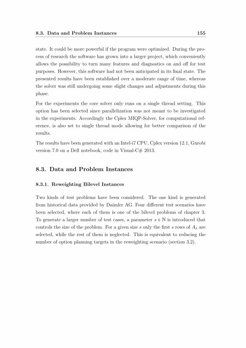
8.3. Data and Problem Instances 155
state. It could be more powerful if the program were optimized. During the pro-
cess of research the software has grown into a larger project, which conveniently
allows the possibility to turn many features and diagnostics on and off for test
purposes. However, this software had not been anticipated in its final state. The
presented results have been established over a moderate range of time, whereas
the solver was still undergoing some slight changes and adjustments during this
phase.
For the experiments the core solver only runs on a single thread setting. This
option has been selected since parallelization was not meant to be investigated
in the experiments. Accordingly the Cplex MIQP-Solver, for computational ref-
erence, is also set to single thread mode allowing for better comparison of the
results.
The results have been generated with an Intel-i7 CPU, Cplex version 12.1, Gurobi
version 7.0 on a Dell notebook, code in Visual-C# 2013.
8.3. Data and Problem Instances
8.3.1. Reweighting Bilevel Instances
Two kinds of test problems have been considered. The one kind is generated
from historical data provided by Daimler AG. Four different test scenarios have
been selected, where each of them is one of the bilevel problems of chapter 3.
To generate a larger number of test cases, a parameter s P N is introduced that
controls the size of the problem. For a given size s only the first s rows of Aλ are
selected, while the rest of them is neglected. This is equivalent to reducing the
number of option planning targets in the reweighting scenario (section 3.2).

8.3. Data and Problem Instances 156
Data Set Dimensions of T Tλ Tλ # Eigenvalues ă 1e-8 Largest EigenvalueData Set 1 156ˆ 156 122 232Data Set 2 156ˆ 156 123 1210Data Set 3 156ˆ 156 122 324Data Set 4 156ˆ 156 122 232
Table 8.1.: Objective Function Characteristics of the Reweighting BilevelInstances
minλ`,λ´,ug ,uh
}Tλpλ` ´ λ´q ´ tλ}2
bλ ´ Aλpλ` ´ λ´q ´ w1` w2
“ 0
pλ` ´ λ´q ` ζ1ě λmin
pλ` ´ λ´q ´ ζ2ď ´λmin
λ`, λ´ ď λmax
0 ď w “ pw1, w2qKζ “ pζ1, ζ2
q ě 0
λ`, λ´ ě 0
(8.1)
The artificial formulation with only positive decision variables is due to the dis-
junctive cuts that are applied to this model. Internally slack variables are intro-
duced, producing a system of only equality constraints. The characteristics of the
test instance objective functions are shown in table 8.1. Although dataset 1 and
dataset 4 have the same characteristics here, they differ in their constraint sets.
During the generation of the objective function the matrices involved are always
scaled if possible, in order to minimize the effects of ill-conditioned data. The
table shows the dimension of the quadratic objective matrix along with numer-
ically zero elements of the spectrum and the maximal eigenvalue. The numbers
show that the objective matrices are rather ill-conditioned. Nevertheless, they
have still been handled well by the instance of the core solver.
8.3.2. QPEC Problems
The other kind is from the MACMPEC website of Sven Leyffer (www.mcs.anl.gov/ leyf-
fer/MacMPEC). The instances qpec-100-1 to qpec-100-4 and qpec-200-1 to qpec-
200-4 have been created by a MATLAB generator as described in [29].

8.3. Data and Problem Instances 157
The generator creates quadratic problems with affine variational inequality con-
straints (AVI-QP):
minpx,y,λqPRn`m`p
fpx, yq
Gx`Hy ` a ď 0
F px, yq ` ETλ “ 0
gpx, yq ď 0, λ ě 0, λTgpx, yq “ 0
F px, yq “ Nx`My ` q
gpx, yq “ Dx` Ey ` b
(8.2)
where fpx, yq “ 12px, yqTP px, yq ` cTx` dTy.
A stationary point in [29] is defined just in the same fashion as a strongly sta-
tionary point in definition 2.10.
The point w˚ “ px˚, y˚, λ˚q is called a stationary point if it is feasible and there
exist multipliers ξ, η, π and ζ such that:
∇xfpx˚, y˚q `GT ξ ´NTη `DTπ “ 0
∇yfpx˚, y˚q `HT ξ ´MTη ` ETπ “ 0
Eη ´ ζ “ 0
ξ ě 0, pGx˚ `Hy˚ ` aqT ξ “ 0
ζi “ 0, @i P αpw˚q
πi ě 0, ζi ě 0, @i P βpw˚q
πi “ 0, @i P γpw˚q
(8.3)
for index sets
αpw˚q “ t1 ď i ď p : λ˚i “ 0 ă ´pDx˚ ` Ey˚ ` bqiu
βpw˚q “ t1 ď i ď p : λ˚i “ ´pDx˚` Ey˚ ` bqi “ 0u
γpw˚q “ t1 ď i ď p : λ˚i ą ´pDx˚` Ey˚ ` bqi “ 0u.
(8.4)
As Jiang and Ralph state, the existence of degenerate indices reflects the com-
plexity of the MPEC. They introduce three types of degeneracy which have cor-
responding input parameters in their QPEC generator.

8.3. Data and Problem Instances 158
Instance nx ny m deg1 deg2 degmqpec-100-1-1 5 100 2 1 20 20qpec-100-1-2 10 100 2 1 20 20qpec-100-1-3 10 100 4 1 20 20qpec-100-1-4 20 100 4 1 20 20qpec-100-2-1 10 200 4 2 40 40qpec-100-2-2 20 200 4 2 40 40qpec-100-2-3 20 200 8 2 40 40qpec-100-2-4 40 200 8 2 40 40
Table 8.2.: Characteristics of the QPEC Test Instances
8.1 Definition ([29] Def 3.1) Suppose w˚ “ px˚, y˚, λ˚q is feasible in 8.2 and
there exist multipliers as in 8.3.
1. An index i is called first-level degenerate if ξi “ pGx˚ `Hy˚ ` aqi “ 0.
2. An index i is called second-level degenerate if i P βpw˚q.
3. A second-level degenerate index i is called mixed degenerate if either πi “ 0
or ζi “ 0.
The instances at hand are a special case of LCP constrained QPs:
minx,y
fpx, yq
Apx, yqT ` a ď 0
0 ď F px, yq “ Nx`My ` qKy ě 0
(8.5)
where x P Rnx , y P Rny , A P Rmˆpnx`nyq and the other dimensions are defined ac-
cordingly. An overview of the characteristics of the QPEC instances is presented
in table 8.2. The numbers of degenerate indices according to Definition 8.1 are
presented in the last three columns.
Note that for some of these instances the algorithm has found slightly lower
objective values than have been published on Sven Leyffer’s site. After a firm
check it is assumed that the solutions are indeed feasible to a tolerance of 1e-8,
to the best of my knowledge.
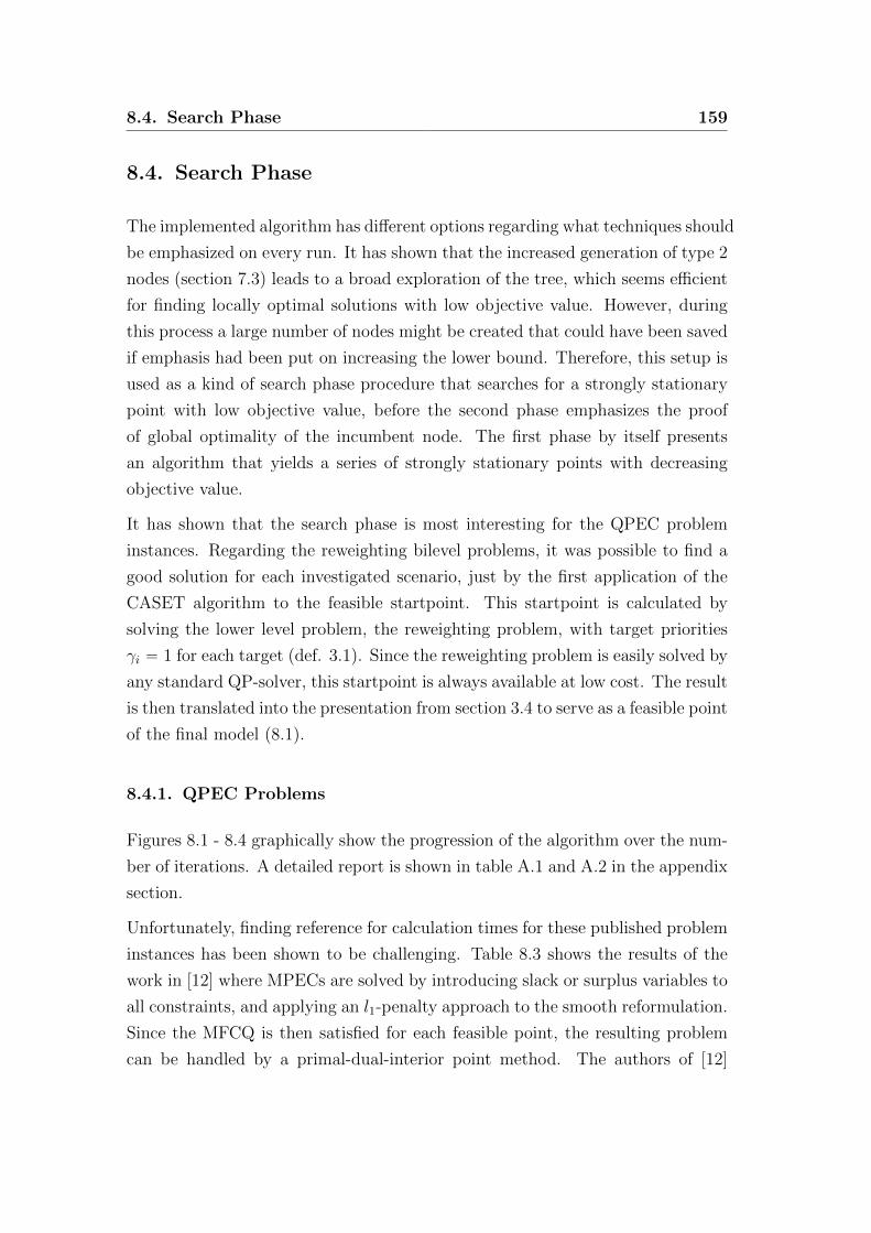
8.4. Search Phase 159
8.4. Search Phase
The implemented algorithm has different options regarding what techniques should
be emphasized on every run. It has shown that the increased generation of type 2
nodes (section 7.3) leads to a broad exploration of the tree, which seems efficient
for finding locally optimal solutions with low objective value. However, during
this process a large number of nodes might be created that could have been saved
if emphasis had been put on increasing the lower bound. Therefore, this setup is
used as a kind of search phase procedure that searches for a strongly stationary
point with low objective value, before the second phase emphasizes the proof
of global optimality of the incumbent node. The first phase by itself presents
an algorithm that yields a series of strongly stationary points with decreasing
objective value.
It has shown that the search phase is most interesting for the QPEC problem
instances. Regarding the reweighting bilevel problems, it was possible to find a
good solution for each investigated scenario, just by the first application of the
CASET algorithm to the feasible startpoint. This startpoint is calculated by
solving the lower level problem, the reweighting problem, with target priorities
γi “ 1 for each target (def. 3.1). Since the reweighting problem is easily solved by
any standard QP-solver, this startpoint is always available at low cost. The result
is then translated into the presentation from section 3.4 to serve as a feasible point
of the final model (8.1).
8.4.1. QPEC Problems
Figures 8.1 - 8.4 graphically show the progression of the algorithm over the num-
ber of iterations. A detailed report is shown in table A.1 and A.2 in the appendix
section.
Unfortunately, finding reference for calculation times for these published problem
instances has been shown to be challenging. Table 8.3 shows the results of the
work in [12] where MPECs are solved by introducing slack or surplus variables to
all constraints, and applying an l1-penalty approach to the smooth reformulation.
Since the MFCQ is then satisfied for each feasible point, the resulting problem
can be handled by a primal-dual-interior point method. The authors of [12]
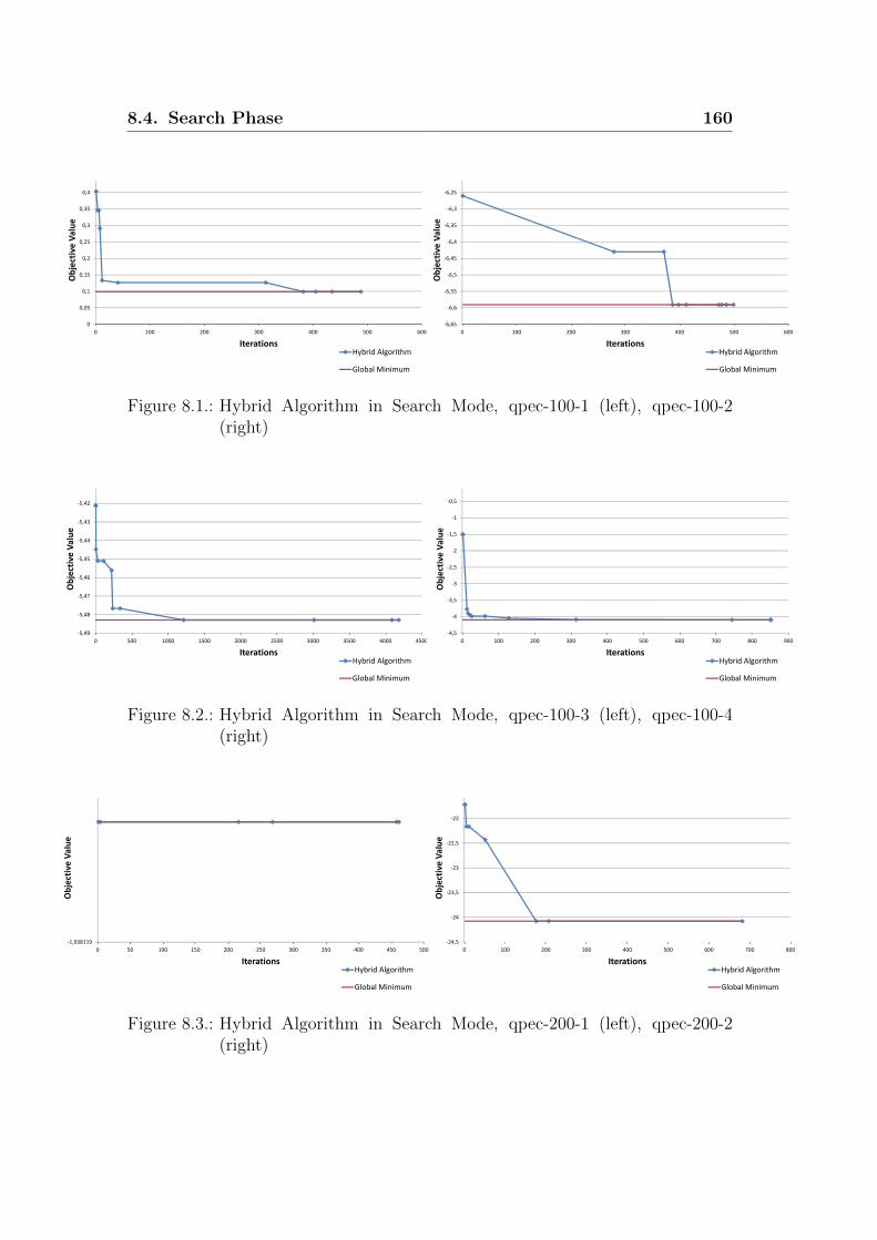
8.4. Search Phase 160
0
0,05
0,1
0,15
0,2
0,25
0,3
0,35
0,4
0,45
0 100 200 300 400 500 600
Ob
ject
ive
Va
lue
IterationsHybrid Algorithm
Global Minimum
-6,65
-6,6
-6,55
-6,5
-6,45
-6,4
-6,35
-6,3
-6,25
-6,2
0 100 200 300 400 500 600
Ob
ject
ive
Va
lue
IterationsHybrid Algorithm
Global Minimum
Figure 8.1.: Hybrid Algorithm in Search Mode, qpec-100-1 (left), qpec-100-2(right)
-5,49
-5,48
-5,47
-5,46
-5,45
-5,44
-5,43
-5,42
-5,41
0 500 1000 1500 2000 2500 3000 3500 4000 4500
Ob
ject
ive
Va
lue
IterationsHybrid Algorithm
Global Minimum
-4,5
-4
-3,5
-3
-2,5
-2
-1,5
-1
-0,5
0
0 100 200 300 400 500 600 700 800 900
Ob
ject
ive
Va
lue
IterationsHybrid Algorithm
Global Minimum
Figure 8.2.: Hybrid Algorithm in Search Mode, qpec-100-3 (left), qpec-100-4(right)
-1,938119
-1,934056
0 50 100 150 200 250 300 350 400 450 500
Ob
ject
ive
Va
lue
IterationsHybrid Algorithm
Global Minimum
-24,5
-24
-23,5
-23
-22,5
-22
-21,5
0 100 200 300 400 500 600 700 800
Ob
ject
ive
Va
lue
IterationsHybrid Algorithm
Global Minimum
Figure 8.3.: Hybrid Algorithm in Search Mode, qpec-200-1 (left), qpec-200-2(right)
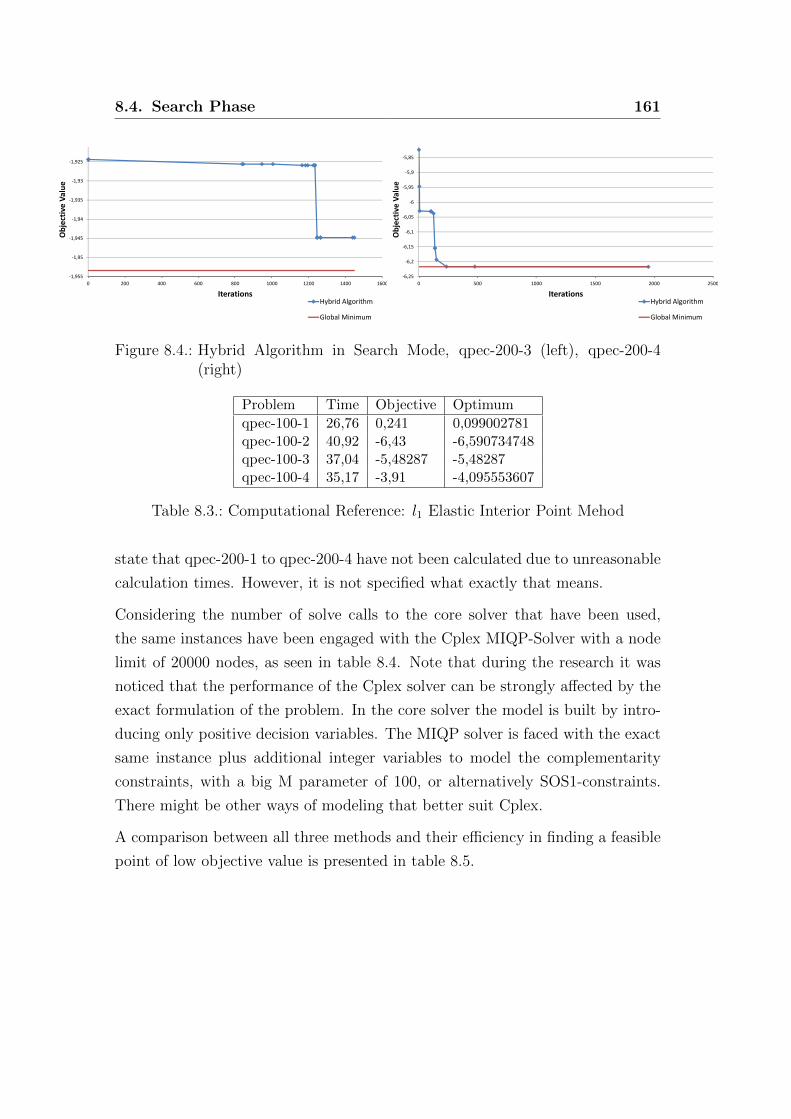
8.4. Search Phase 161
-1,955
-1,95
-1,945
-1,94
-1,935
-1,93
-1,925
-1,92
0 200 400 600 800 1000 1200 1400 1600
Ob
ject
ive
Va
lue
IterationsHybrid Algorithm
Global Minimum
-6,25
-6,2
-6,15
-6,1
-6,05
-6
-5,95
-5,9
-5,85
-5,8
0 500 1000 1500 2000 2500
Ob
ject
ive
Va
lue
IterationsHybrid Algorithm
Global Minimum
Figure 8.4.: Hybrid Algorithm in Search Mode, qpec-200-3 (left), qpec-200-4(right)
Problem Time Objective Optimum
qpec-100-1 26,76 0,241 0,099002781qpec-100-2 40,92 -6,43 -6,590734748qpec-100-3 37,04 -5,48287 -5,48287qpec-100-4 35,17 -3,91 -4,095553607
Table 8.3.: Computational Reference: l1 Elastic Interior Point Mehod
state that qpec-200-1 to qpec-200-4 have not been calculated due to unreasonable
calculation times. However, it is not specified what exactly that means.
Considering the number of solve calls to the core solver that have been used,
the same instances have been engaged with the Cplex MIQP-Solver with a node
limit of 20000 nodes, as seen in table 8.4. Note that during the research it was
noticed that the performance of the Cplex solver can be strongly affected by the
exact formulation of the problem. In the core solver the model is built by intro-
ducing only positive decision variables. The MIQP solver is faced with the exact
same instance plus additional integer variables to model the complementarity
constraints, with a big M parameter of 100, or alternatively SOS1-constraints.
There might be other ways of modeling that better suit Cplex.
A comparison between all three methods and their efficiency in finding a feasible
point of low objective value is presented in table 8.5.

8.5. Global Optima 162
Problem Nodes Calculated Incumbent Objectiveqpec-100-1 20000 -1 +infinityqpec-100-2 20000 5328 -5,82511qpec-100-3 20000 352 -5,44460qpec-100-4 3321 1464 -4,09555qpec-200-1 20000 8985 -1,90255qpec-200-2 20000 -1 +infinityqpec-200-3 20001 375 5,43762qpec-200-4 20000 10464 -5,81456
Table 8.4.: Computational Reference: Cplex 12.1 MIQP-Solver
Cplex l1 Elastic Int. Point M. Hybrid Alg.Instance Time Obj. Val. Time Obj. Val. Time Obj. Val.qpec-100-1 11,12s 8 26,76s 0,241 11,32s 0,09900qpec-100-2 12,01s -5,9826 40,92s -6,43 12,06s -6,59073qpec-100-3 12,00s -5,4446 37,04s -5,48287 12,19s -5,47665qpec-100-4 3,46s -4,0956 35,17s -3,91 12,04s -4,08768
Table 8.5.: Performance Indicators
8.5. Global Optima
8.5.1. QPEC Problems
During the research, one of the major observations was that branch-and-bound
trees generated by the hybrid algorithm did not have very beneficial properties
in proving optimality for any of the QPEC instances. It seems that splitting
from a strongly stationary point or an A-stationary point (or from a partially
feasible point that is stationary on one of the nodes) creates an unnecessarily
large number of new nodes, which is most likely due to the degrees of degen-
eracy (def. 8.1) these problems have been generated with. It has shown that
the implemented methods using disjunctive cuts, gradient based constraints or
Lagrange lower bounds have not been able to reduce the size of the tree over all.
The exploration of this tree comes with the upside that many locally optimal
solutions are found in the process. In regards of the proof of global optimality
however, the approach seems to be counterproductive. The hybrid algorithm can
still solve the instances in reasonable time, compared to the Cplex MIQP solver
or most infeasible branching, although it always comes in second. Most infea-
sible branching, on the other hand, has shown to be quite effective. Table 8.6
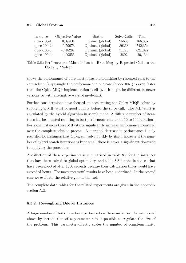
8.5. Global Optima 163
Instance Objective Value Status Solve Calls Timeqpec-100-1 0,09900 Optimal (global) 25685 166,35sqpec-100-2 -6,59073 Optimal (global) 89363 742,35sqpec-100-3 -5,48287 Optimal (global) 71175 621,09sqpec-100-4 -4,09555 Optimal (global) 2802 20,13s
Table 8.6.: Performance of Most Infeasible Branching by Repeated Calls to theCplex QP Solver
shows the performance of pure most infeasible branching by repeated calls to the
core solver. Surprisingly the performance in one case (qpec-100-1) is even faster
than the Cplex MIQP implementation itself (which might be different in newer
versions or with alternative ways of modeling).
Further considerations have focused on accelerating the Cplex MIQP solver by
supplying a MIP-start of good quality before the solve call. The MIP-start is
calculated by the hybrid algorithm in search mode. A different number of itera-
tions has been tested resulting in best performances at about 10 to 100 iterations.
For some instances these MIP-starts significantly increase performance measured
over the complete solution process. A marginal decrease in performance is only
recorded for instances that Cplex can solve quickly by itself, however if the num-
ber of hybrid search iterations is kept small there is never a significant downside
to applying the procedure.
A collection of these experiments is summarized in table 8.7 for the instances
that have been solved to global optimality, and table 8.8 for the instances that
have been aborted after 1800 seconds because their calculation times would have
exceeded hours. The most successful results have been underlined. In the second
case we evaluate the relative gap at the end.
The complete data tables for the related experiments are given in the appendix
section A.2.
8.5.2. Reweighting Bilevel Instances
A large number of tests have been performed on these instances. As mentioned
above by introduction of a parameter s it is possible to regulate the size of
the problem. This parameter directly scales the number of complementarity

8.5. Global Optima 164
Search Iterations 10 50 100 200 500 1000Difference qpec-100-1 -97% -97% -97% -97% -96% -95%in Solution qpec-100-2 5% 3% 3% 3% -6% -4%Time qpec-100-3 -93% -93% -93% -93% -91% -90%
qpec-100-4 8% 19% 38% 76% 277% 661%qpec-200-1 -63% -40% -4% 80% 551% 668%qpec-200-2 0% 0% 0% 0% 0% 0%qpec-200-3 0% 0% 0% 0% 0% 0%qpec-200-4 0% 0% 0% 0% 0% 0%Sum -240% -209% -154% -31% 634% 1140%Mean -30% -26% -19% -4% 79% 142%
Table 8.7.: Cplex MIQP Solver in Classic Branch-and-Bound Mode with MIP-Starts provided by the Hybrid Algorithm in Search Mode
Search Iterations 0 10 50 100 200 500 1000Cplex qpec-200-2 8 0,464 0,465 0,464 0,467 0,476 0,494Relative qpec-200-3 0,511 0,322 0,320 0,323 0,323 0,338 0,339Gap qpec-200-4 0,132 0,134 0,135 0,136 0,146 0,141 0,152
Table 8.8.: Cplex MIQP Solver in Classic Branch-and-Bound Mode with MIP-Starts provided by the Hybrid Algorithm in Search Mode
constraints which is 2s. An instance is therefore defined by the combination of
the selected data set and the problem size parameter s.
The individual experiments also differ in the setup of the involved modules. Some
have been conducted with inclusion of the search phase (see 8.4) that is sepa-
rated from the following second phase. The LP/MIP-feasibility approach is used
with different thresholds. In contrary to these cases, it has also been turned off
completely for some runs. In this case, if the algorithm initializes a call to the
CASET subroutine with infeasible startpoint, the algorithm will simply relax all
the complementary indices that are not fixed. The gradient based constraints
and disjunctive cuts have been generated in varying frequency and different total
maximum number, which had no significant influence on performance. This is
why there will be little emphasis on the point of cut generation in the following
tables. However completely turning constraint and cut generation on or off has
created more noticeable effects.

8.5. Global Optima 165
Most successful Results
Experiments have shown that the algorithm performs most successfully on the
reweighting bilevel MPECs with the variable bound constraints as described in
section 7.6.2. The column names are explained below. The results are shown
in table 8.9. Every instance has been solved by the Cplex MIQP solver and the
hybrid algorithm, and globally optimal solutions with coinciding objective values
have always been found. The most successful results occurred with a parameter
setting where the cut generation module and Lagrange lower bounds have been
turned off. This shows of course that their application is not always helpful in
the matter of performance. For two of the instances with size s “ 90 the hybrid
algorithm performs faster than the Cplex MIQP solver. Although there is only an
increase in 20 complementarity constraints from s “ 80 to s “ 90 we note that the
complexity of MPECs grows exponentially with the number of complementartiy
constraints in general. For s “ 100, calculations have been aborted due to heavily
increased calculation times in both solvers (aborted after one or more hours due
to the lack of progress). For smaller instances it is very likely that the generated
overhead in the hybrid algorithm is too large.
The table columns are defined as follows:
• s - Problem size, number of complemen-
tary constraints is 2s
• Ph1 It. - Iterations of the search phase
• Ph1 Obj. - Objective value after search
phase of the algorithm
• UB - Upper bound of the hybrid algo-
rithm
• LB - Lower bound of the hybrid algo-
rithm
• C. Obj. - Cplex Objective value
• C. Inc. - Cplex incumbent node
• It. - The number of iterations of the
hybrid solver
• S. Calls - Calls to the QP/LP-Solver of
the core solver
• t - Solving time of the hybrid solver
• Feas. - Whether the feasibility unit was
active
• M. Infeas. - Whether the BBASET
branching from a stationary point was
performed by the largest negative dual
or the most infeasibel index (see section
7.6.3)
• CASET - Whether the CASET algo-
rithm and related features were uti-
lized at all; if not then most infeasible
branching is used
• F. MIPs - The number of MIP calls in
the feasibility unit
• F. LPs - The number of LP calls in the
feasibility unit

8.5. Global Optima 166
Data Set s F. MIPs LPs C. Nodes C. Inc. Ph1 It. Ph1 Obj. UB LB It. S. Calls t C. TimeData Set 1 90 5177 325424 353609 330308 90 0,63844 0,63108 0,63108 5177 5177 2438,36 692,66Data Set 2 90 1001 34695 138062 133597 90 1,16704 1,16704 1,16704 1001 1001 235,1 252,20
Data Set 3 90 535 21439 147698 65202 90 0,71833 0,71833 0,71833 535 535 162,48 262,35
Data Set 4 90 2869 113973 176956 141122 90 0,84223 0,84223 0,84223 2869 2869 818,7 337,66Data Set 1 80 1935 108406 94296 14202 80 0,6384 0,6266 0,6266 1935 1935 580,22 143,64Data Set 2 80 747 23452 29274 29170 80 1,15887 1,15887 1,15887 747 747 124,27 44,37Data Set 3 80 463 17602 7316 3656 80 0,71464 0,71464 0,71464 463 463 102,77 10,55Data Set 4 80 2561 93062 31035 30526 80 0,89039 0,89039 0,89039 2561 2561 518,85 50,22
Table 8.9.: Hybrid Algorithm compared to Cplex MIQP Solver on Global Optimafor the Reweighting Bilevel MPEC
• Dual Bnds. - The number of Lagrange
dual bounds that have been calculated
• Cuts - The total number of disjunctive
cuts that have been generated
• LPs - LP calls in the variable bound
constraint generation (alg. 18)
Additional Results
Further results show the performance of the hybrid solver for different settings
of the modules. All instances have been aborted after a certain time limit. In
those cases where lower and upper bound do not coincide the time limit has been
reached. The time limit depends on the problem size and can be seen in the
tables (150 seconds for data set 1 with s “ 50).
Tables 8.10 (and in appendix: A.6, A.7, A.8, A.9 and A.10) present the results.
A short analysis of the results shows that the calculation of the Lagrange lower
bounds is inefficient with the current implementation. The solution of the non-
convex subproblems takes more time than the calculated lower bounds save in
the branch-and-bound framework. Further research might try to solve these
subproblems with an approach that is more sophisticated from the perspective of
programming, or use an implementation of the BBASET algorithm as has been
proposed before. It might also be possible to find a better indicator that yields an
improvement on the selection of the nodes for which these bounds are calculated.
A positive observation is that the hybrid branch-and-bound algorithm produces
fewer nodes compared to the Cplex MIQP solver for several instances.

8.5. Global Optima 167
Data Set s Ph1 Obj. UB LB It. S. Calls t Feas. M. Infeas. CASET F. MIPs F. LPs Dual Bnds. CutsData Set 1 50 0,60451 0,60451 2381 2736 53,62 n y y 0 64Data Set 1 50 0,60451 0,60451 0,60451 2381 2735 58,49 n y y 0 64Data Set 1 50 0,60451 0,60451 2376 2657 61,92 n y y 0 0Data Set 1 50 0,60451 0,60451 0,60451 2376 2656 64,29 n y y 0 0Data Set 1 50 0,60451 0,60451 4015 4324 85,18 n n y 0 52Data Set 1 50 0,60451 0,60451 0,60451 4015 4323 86,14 n n y 0 52Data Set 1 50 0,60451 0,60451 4124 4381 92,68 n n y 0 0Data Set 1 50 0,60451 0,60451 0,60451 4124 4380 96,2 n n y 0 0Data Set 1 50 0,60451 0,60451 0,60451 6757 6765 116,61 n 0 8Data Set 1 50 0,60451 0,60451 6847 6847 122,01 n 0 0Data Set 1 50 0,60451 0,60451 0,60451 6847 6847 138,58 n 0 0Data Set 1 50 0,60451 0,60451 6847 6847 142,53 n 0 0Data Set 1 50 0,60451 0,59889 2838 4562 150,01 y n y 4428 1509 0 79Data Set 1 50 0,60692 0,60409 6560 6559 150,02 n 696 0Data Set 1 50 0,60692 0,60358 6298 6297 150,09 n 434 0Data Set 1 50 0,60451 0,60451 0,5991 2916 4642 153,6 y n y 4506 1509 0 79
Table 8.10.: Hybrid Algorithm on the Reweighting Bilevel MPEC - Data Set 1
Data Set s Initial Part Match Optimized Part Match Quality IncreasePositive Variables Relaxed Positive Variables Relaxed
Data Set 1 50 73,77136 73,77133 60,17119 60,17122 18,44 %Data Set 2 20 177,24619 177,24627 150,62900 150,62903 15,02%Data Set 2 50 178,26510 178,26508 140,39935 140,39981 21,24%Data Set 3 30 103,50506 103,50506 87,95038 87,95038 15,03%Data Set 4 20 154,94687 154,94657 128,67834 128,67847 16,95%Data Set 4 40 152,27729 152,27727 117,35046 117,35040 22,94%
Table 8.11.: Upper Level Objective of the Lower Level Solution before and afterthe Bilevel Optimization

8.6. Conclusion 168
Practical Use for Demand Forecast Calculations
Although so far the technical evaluation of the algorithm has been focused on,
table 8.11 presents the evaluation of the lower level (i.e. reweighting) solution
point in the original ex-post objective function T (section 3.2). The bilevel model
which is subject to optimization has undergone different modifications from the
original ex-post problem to its final state. The numbers reflect the final use of the
calculations. Extra columns have been added solving the lower level problem with
and without positivity constraints on the variables (in reference to section 3.4.1).
As table 8.11 presents, the solution of the bilevel problem yields a corresponding
reweighting (i.e. lower level) point that always has a part match of better quality,
if evaluated in the ex-post situation. The increase lies at 15 to 23 percent.
Whether resulting target prioritizations can be used in practice needs to be in-
vestigated in a long term experiment. One particular result might be useful in
a training scenario that has been built from a specific dataset. However, we
cannot conclude that this prioritization does also yield a quality increase in de-
mand forecasts for future time periods, although the concept of training scenarios
depends on the occurrence of this expected effect. Thus, prioritization is only de-
sirable if the quality increase shows some significant stability over time. Whether
this method will be applied to further reweighting calculations in actual demand
forecasts is still up for discussion, and might be the content for future projects.
8.6. Conclusion
The experiments have shown that the CASET algorithm is indeed a valuable tool
for operating on a set of linear constraints and linear complementarity constraints
with a convex objective function. Expanding this local search method to the
whole solution space by considering yet the same dual multipliers as CASET
itself, the idea of the BBASET algorithm is intuitive and bears great potential
for the instances at hand. The hybrid algorithm has eliminated the downside
of working with non-convex problems in order to restore feasibility. This makes
the algorithm more accessible to users from outside of the theoretical field, since
professional optimization software is already in a state of high reliability.
The search phase of the algorithm was successfully applied to the complete set

8.6. Conclusion 169
of experiments. Regarding the proof of optimality, the investigation shows that
branching by the most infeasible index can be reliable to a certain extent. Off-the-
shelf implementations such as Cplex are overall preferable but their performance
can be increased by supplying startpoints with the search method of the hybrid
algorithm without any risk. For a number of experiments (with the reweighting
bilevel MPEC instances) the hybrid algorithm manages to reduce the number of
solve calls to the core QP-solver. Furthermore, the results show that for a small
number of experiments the hybrid algorithm is faster. Given a more advanced
implementation, further tuning and experiments and a greater set of instances,
this might be the subject of future research.
A theoretical challenge is the development of further indicators that guide the al-
gorithm in analysis of the given problem instance, or the incorporation of already
existing techniques in this area. This would yield an increase in flexibility and
reliability of the algorithm. In the current state, the behaviour of the algorithm is
massively dependent on the parameter set that has been selected beforehand, and
that controls the subroutines of the individual modules. Problem preprocessing
techniques should be utilized, incorporating more information that arises during
the solution process and depends on the given problem structure.
Regarding the use in the presented business application, the bilevel optimization
has shown that the quality of reweighting results could be reasonably improved
by utilization of favorable option planning target prioritizations. The implemen-
tation is able to find solutions of high quality in calculation times that are little
to the user, and is ready to be applied to ex-post data.
Bibliography
1 Anh, P. N. and Muu, L. D. (2006). Lagrangian duality algorithms for find-
ing a global optimal solution to mathematical programs with affine equilibrium
constraints. Nonlinear Dynamics and Systems Theory, 6(3):225–244.
2 Audet, C., Savard, G., and Zghal, W. (2007). New branch-and-cut algorithm
for bilevel linear programming. Journal of Optimization Theory and Applica-
tions, 134(2):353–370.
3 Balas, E. and Perregaard, M. (2002). Lift-and-project for mixed 0–1 program-
ming: recent progress. Discrete Applied Mathematics, 123(1–3):129 – 154.
4 Bard, J. F. (1998). Practical Bilevel Optimization: Algorithms and Applica-
tions. Kluwer Academic Publishers.
5 Bazaraa, M. S., Sherali, H. D., and Shetty, C. M. (2006). Nonlinear Program-
ming: Theory and Algorithms, 3rd Edition. Wiley.
6 Belotti, P., Kirches, C., Leyffer, S., Linderoth, J., Luedtke, J., and Mahajan,
A. (2013). Mixed-integer nonlinear optimization. Acta Numerica, 22:1–131.
7 Ben-Tal, A., Eiger, G., and Gershovitz, V. (1994). Global minimization by
reducing the duality gap. Mathematical Programming, 63(1):193–212.
8 Bolzon, G., Ghilotti, D., and Maier, G. (1997). Parameter Identification of the
Cohesive Crack Model, pages 213–222.
9 Brabazon, P. G., MacCarthy, B., Woodcock, A., and Hawkins, R. W. (2010).
Mass customization in the automotive industry: Comparing interdealer trading
and reconfiguration flexibilities in order fulfillment. Production and Operations
Management, 19(5):489–502.
10 Calamai, P. and More, J. (1987). Projected gradient methods for linearly
constrained problems. Mathematical Programming, 39(1):93–116.
170

Bibliography 171
11 Cottle, R. W., Pang, J.-S., and Venkateswaran, V. (1989). Sufficient matrices
and the linear complementarity problem. Linear Algebra and its Applications,
114:231–249. Special Issue Dedicated to Alan J. Hoffman.
12 Coulibaly, Z. and Orban, D. (2012). An l1 elastic interior-point method for
mathematical programs with complementarity constraints. SIAM Journal on
Optimization, 22(1):187–211.
13 D., K. (1985). On the lipschitz behavior of optimal solutions in parametric
problems of quadratic optimization and linear complementarity. Optimization,
16(6):819–831.
14 D., M. L. and V., Q. N. (2007). On branch-and-bound algorithms for global
optimal solutions to mathematical programs with affine equilibrium constraints.
Vietnam Journal of Mathematics 35:4(2007) 523-539, 35(4):523–539.
15 Dempe, S. (2002). Foundations of Bilevel Programming. Kluwer Academic
Publishers, New York.
16 Ehrgott, M. (2005). Multicriteria optimization. Springer-Verlag, Berlin, sec-
ond edition.
17 Falk, J. E. (1969). Lagrange multipliers and nonconvex programs. SIAM
Journal on Control, 7(4):534–545.
18 Fang, H., Leyffer, S., and Munson, T. (2012). A pivoting algorithm for linear
programming with linear complementarity constraints. Optimization Methods
and Software, 27(1):89–114.
19 Fernandes, L., Friedlander, A., Guedes, M., and Judice, J. J. (2001). Solution
of a general linear complementarity problem using smooth optimization and
its application to bilinear programming and LCP. Applied Mathematics and
Optimization, 43(1):1–19.
20 Fletcher, R., Leyffer, S., Ralph, D., and Scholtes, S. (2006). Local convergence
of SQP methods for mathematical programs with equilibrium constraints. SIAM
Journal on Optimization, 17(1):259–286.
21 Gale, D. N. and Nikaido, H. (1965). The jacobian matrix and global univa-
lence of mappings. Mathematische Annalen, 159(2):81–93.
Bibliography 172
22 Geiger, C. and Kanzow, C. (2002). Theorie und Numerik restringierter Op-
timierungsaufgaben. Springer-Verlag Berlin Heidelberg.
23 Horst, R. and Tuy, H. (1996). Global Optimization - Deterministic Ap-
proaches, volume 3. Springer-Verlag Berlin Heidelberg.
24 Hu, J., Mitchell, J. E., Pang, J.-S., Bennett, K. P., and Kunapuli, G. (2008).
On the global solution of linear programs with linear complementarity con-
straints. SIAM Journal on Optimization, 19(1):445–471.
25 Hu, X. M. and Ralph, D. (2004). Convergence of a penalty method for
mathematical programming with complementarity constraints. Journal of Op-
timization Theory and Applications, 123(2):365–390.
26 Ibaraki, T. (1971). Complementary programming. Operations Research,
19(6):1523–1529.
27 Ibaraki, T. (1973). The use of cuts in complementary programming. Opera-
tions Research, 21(1):353–359.
28 Jeroslow, R. G. (1978). Cutting-planes for complementarity constraints.
SIAM Journal on Control and Optimization, 16(1):56–62.
29 Jiang, H. and Ralph, D. (1999). QPECgen, a MATLAB generator for math-
ematical programs with quadratic objectives and affine variational inequality
constraints. Comput. Optim. Appl., 13(1-3):25–59.
30 Judice, J. J. (2012). Algorithms for linear programming with linear comple-
mentarity constraints. Top, 20(1):4–25.
31 Judice, J. J. (2014). Optimization with linear complementarity constraints.
Pesquisa Operacional, 34:559–584.
32 Judice, J. J., Faustino, A. M., and Ribeiro, I. M. (2002). On the solution of
NP-hard linear complementarity problems. Top, 10(1):125–145.
33 Judice, J. J. and Mitra, G. (1988). Reformulation of mathematical program-
ming problems as linear complementarity problems and investigation of their
solution methods. Journal of Optimization Theory and Applications, 57(1):123–
149.

Bibliography 173
34 Judice, J. J., Sherali, H. D., Ribeiro, I. M., and Faustino, A. M. (2006). A
complementarity-based partitioning and disjunctive cut algorithm for mathe-
matical programming problems with equilibrium constraints. Journal of Global
Optimization, 36(1):89–114.
35 Judice, J. J., Sherali, H. D., Ribeiro, I. M., and Faustino, A. M. (2007).
Complementarity active-set algorithm for mathematical programming problems
with equilibrium constraints. Journal of Optimization Theory and Applications,
134(3):467–481.
36 Kallrath, J. (2002). Gemischt-Ganzzahlige Optimierung: Modellierung in Der
Praxis: Mit Fallstudien aus Chemie, Energiewirtschaft, Metallgewerbe, Produk-
tion und L]ogistik. Springer Fachmedien Wiesbaden.
37 Kanzow, C. and Schwartz, A. (2014). Convergence properties of the inexact
lin-fukushima relaxation method for mathematical programs with complemen-
tarity constraints. Computational Optimization and Applications, 59(1):249–
262.
38 Kappler, J. (2010). Dissertation: Robuste intervallbasierte Primar- und
Sekundarsbedarfsplanung in automobilen Neuproduktprojekten. University of
Clausthal.
39 Kellerer, H., Pferschy, U., and Pisinger, D. (2013). Knapsack Problems.
Springer Berlin Heidelberg.
40 Kinderlehrer, D. and Stampacchia, G. (2000). An Introduction to Variational
Inequalities and Their Applications. Society for Industrial and Applied Mathe-
matics.
41 Kojima, M., Megiddo, N., Noma, T., and Yoshise, A. (1991). A Unified
Approach to Interior Point Algorithms for Linear Complementarity Problems.
Springer-Verlag.
42 Konnov, I. and Laitinen, E. (2002). Theory and applications of variational
inequalities. Preprint, April 2002.
43 Korner, F. (1983). An efficient branch and bound algorithm to solve the
quadratic integer programming problem. Computing, 30(3):253–260.

Bibliography 174
44 Korner, F. (1988). A new branching rule for the branch and bound algorithm
for solving nonlinear integer programming problems. BIT Numerical Mathemat-
ics, 28(3):701–708.
45 Korner, F. (1982). Untersuchungen uber eine gunstige Verzweigungsreihen-
folge der Variablen bei Branch and Bound-Verfahren. Mathematische Opera-
tionsforschung und Statistik. Series Optimization, 13(2):221–229.
46 Korner, F. (1985). Integer quadratic optimization. European Journal of
Operational Research, 19(2):268–273.
47 Lee, G. M., Tam, N. N., and Yen, N. D. (2005). Quadratic Programming and
Affine Variational Inequalities. Springer US.
48 Lee, G. M., Tam, N. N., and Yen, N. D. (2006). Continuity of the solution
map in quadratic programs under linear perturbations. Journal of Optimization
Theory and Applications, 129(3):415–423.
49 Leyffer, S. and Munson, T. S. (2007). A globally convergent filter method for
MPECs. Preprint ANL/MCS-P1457-0907.
50 Lindemann, U., Reichwald, R., and Zah, M. F. (2006). Individualisierte
Produkte - Komplexitat beherrschen in Entwicklung und Produktion. Springer-
Verlag Berlin Heidelberg.
51 Luo, Z., Pang, J.-S., and Ralph, D. (1998). Piecewise Sequential Quadratic
Programming for Mathematical Programs with Nonlinear Complementarity Con-
straints, pages 209–229.
52 Mangasarian, O. L. (1965). Pseudo-convex functions. Journal of the Society
for Industrial and Applied Mathematics, 3(2):281–290.
53 Mangasarian, O. L. (1995). The linear complementarity problem as a sepa-
rable bilinear program. Journal of Global Optimization, 6(2):153–161.
54 Martello, S. and P., T. (2003). An exact algorithm for the two-constraint 0-1
knapsack problem. Operations Research, 51(5):826–835.
55 Mitchell, J. E., Pang, J.-S., and Yu, B. (2012). Obtaining Tighter Relaxations
of Mathematical Programs with Complementarity Constraints, pages 1–23.

Bibliography 175
56 Morrison, D. R., Jacobson, S. H., Sauppe, J. J., and Sewell, E. C. (2016).
Branch-and-bound algorithms: A survey of recent advances in searching, branch-
ing, and pruning. Discrete Optimization, 19:79–102.
57 Murtagh, B. A. and Saunders, M. A. (1983). Minos 5.5 user’s guide. http:
//www.sbsi-sol-optimize.com/index.htm. Accessed: 2017-08-23.
58 Myerson, R. (1999). Nash equilibrium and the history of economic theory.
Journal of Economic Literature, 37(3):1067–1082.
59 Nocedal, J. and Wright, S. (2006). Numerical Optimization. Springer-Verlag
New York.
60 Nogales, M., Francisco, J., Miguel, A., Friedlander, M., and Scholtes, S.
(2004). An interior-point method for mpecs based on strictly feasible relaxations.
DES - Working Papers. Statistics and Econometrics. WS ws042408, Universidad
Carlos III de Madrid. Departamento de Estadıstica.
61 Obuchowska, W. T. and Murty, K. G. (2001). Cone of recession and un-
boundedness of convex functions. European Journal of Operational Research,
133(2):409 – 415. Multiobjective Programming and Goal Programming.
62 Ralph, D. and J., W. S. (2004). Some properties of regularization and penal-
ization schemes for MPECs. Optimization Methods and Software, 19(5):527–556.
63 Scheel, H. and S., S. (2000). Mathematical programs with complementarity
constraints: Stationarity, optimality, and sensitivity. Mathematics of Operations
Research, 25(1):1–22.
64 Scholtes, S. (2000). Convergence properties of a regularization scheme for
mathematical programs with complementarity constraints. SIAM J. on Opti-
mization, 11(4):918–936.
65 Sherali, H. D. and Shetty, C. M. (1980). Optimization with Disjunctive Con-
straints. Springer-Verlag Berlin Heidelberg.
66 Shor, N. Z. and Stetsyuk, P. I. (2002). Lagrangian bounds in multiextremal
polynomial and discrete optimization problems. Journal of Global Optimization,
23(1):1–41.

Bibliography 176
67 Staeblein, T. (2007). Dissertation: Integrierte Planung des Materialbedarfs
bei kundenauftragsorientierter Fertigung von komplexen und variantenreichen
Serienprodukten. University of Clausthal.
68 Stephan, D. (2003). Annotated bibliography on bilevel programming and
mathematical programs with equilibrium constraints. Optimization, 52(3):333–
359.
69 von Stackelberg, H., Bazin, D., Hill, R., and Urch, L. (2010). Market Structure
and Equilibrium. Springer Berlin Heidelberg.
70 Website. Collection of mathematical programs with equilibrium constraints
(mpec) test problems in ampl. www.mcs.anl.gov/~leyffer/MacMPEC. Ac-
cessed: 2017-08-23.
71 Website. Gurobi R©. http://www.gurobi.com/resources/
getting-started/mip-basics. Accessed: 2017-08-23.
72 Website. Mercedes-Benz R©. http://www.mercedes-benz.de/. Accessed:
2017-08-23.
73 Website. Organization of Motor Vehicle Manufacturers (OICA). http://
www.oica.net/category/economic-contributions/. Accessed: 2017-08-23.
74 Ye, J. J. (2005). Necessary and sufficient optimality conditions for mathemat-
ical programs with equilibrium constraints. Journal of Mathematical Analysis
and Applications, 307(1):350–369.
75 Zhang, J. and Liu, G. (2001). A new extreme point algorithm and its ap-
plication in PSQP algorithms for solving mathematical programs with linear
complementarity constraints. Journal of Global Optimization, 19(4):345–361.

Appendix
177

A. Computational Results
A.1. Search Phase Iterations
The iterations of the search phase on the QPEC problems are shown in table A.1
and A.2.
A.2. CPLEX MIQP Solver with MIP-Starts provided by
the Hybrid Algorithm in Search Mode
Appending section 8.5: The various experiments differ in in the following char-
acteristics:
• The number of iterations of the hybrid algorithm in search mode used to
calculate the MIP-start (where no iterations means that CPLEX just runs
by itself);
• Modeling the problem with SOS1-constraints and positive variables or al-
ternatively modeling with binary variables and a big-M parameter of 100.
If SOS1-constraints are used the set of active constraints that is found at
the solution of the hybrid algorithm in search phase is prioritized;
• CPLEX search mode which can either be set to Classic Branch-and-Bound
or Dynamic Search.
The classic branch-and-bound option has been considered to blend out some of
the features that CPLEX uses internally to boost performance. A time limit of
1800 seconds was imposed on all calculations. Runs that have been aborted are
evaluated by their relative gap that remains. Elements of best performance have
been underlined.
The results are presented in table A.3 - A.5.
178

A.2. CPLEX MIQP Solver with MIP-Starts provided by the Hybrid
Algorithm in Search Mode179
Problem Iteration QP/LP Solve Calls Objective Global Minimum Time in s
qpec-100-1 1 6 0,403458695 0,099002781 0,0198405qpec-100-1 4 48 0,345441094 0,099002781 0,1449084qpec-100-1 6 57 0,345441094 0,099002781 0,1906315qpec-100-1 8 83 0,291060044 0,099002781 0,2589583qpec-100-1 12 117 0,132963869 0,099002781 0,3572013qpec-100-1 41 283 0,1265236 0,099002781 0,9942933qpec-100-1 313 2250 0,1265236 0,099002781 9,219647qpec-100-1 382 2578 0,099002781 0,099002781 11,3285979qpec-100-1 405 2667 0,099002781 0,099002781 11,9640877qpec-100-1 435 2817 0,099002781 0,099002781 12,8642272qpec-100-1 488 3176 0,099002781 0,099002781 14,834412
qpec-100-2 1 59 -6,260490064 -6,590734748 0,1787396qpec-100-2 279 1505 -6,430055819 -6,590734748 8,3977674qpec-100-2 371 1864 -6,430055819 -6,590734748 11,3360284qpec-100-2 387 1959 -6,590734748 -6,590734748 12,0561706qpec-100-2 398 2010 -6,590734748 -6,590734748 12,5722964qpec-100-2 412 2051 -6,590734748 -6,590734748 13,0190164qpec-100-2 472 2297 -6,590734748 -6,590734748 15,3257387qpec-100-2 477 2321 -6,590734748 -6,590734748 15,5618755qpec-100-2 486 2347 -6,590734748 -6,590734748 15,8762203qpec-100-2 499 2399 -6,590734748 -6,590734748 16,7112063
qpec-100-3 1 53 -5,421196864 -5,482874548 0,2911508qpec-100-3 2 56 -5,421196864 -5,482874548 0,3185076qpec-100-3 4 67 -5,44477174 -5,482874548 0,4012306qpec-100-3 30 309 -5,451074667 -5,482874548 1,6127008qpec-100-3 110 869 -5,451074667 -5,482874548 4,8334322qpec-100-3 220 1352 -5,456089005 -5,482874548 8,0817879qpec-100-3 235 1416 -5,476649453 -5,482874548 8,5302009qpec-100-3 338 2044 -5,476649453 -5,482874548 12,1926401qpec-100-3 1214 7834 -5,482874548 -5,482874548 51,0554487
qpec-100-4 1 28 -1,503267455 -4,095553607 0,0912504qpec-100-4 2 31 -1,503267455 -4,095553607 0,1131668qpec-100-4 13 84 -3,771462838 -4,095553607 0,3801813qpec-100-4 16 143 -3,899213136 -4,095553607 0,5873441qpec-100-4 21 177 -3,946745341 -4,095553607 0,7356504qpec-100-4 26 200 -3,982117798 -4,095553607 0,8632765qpec-100-4 63 318 -3,982117798 -4,095553607 1,6549866qpec-100-4 128 513 -4,045289875 -4,095553607 3,5188577qpec-100-4 314 1360 -4,087684677 -4,095553607 12,0432667qpec-100-4 744 3106 -4,095553607 -4,095553607 34,8899223qpec-100-4 850 3402 -4,095553607 -4,095553607 40,6035238qpec-100-4 852 3410 -4,095553607 -4,095553607 40,8464446qpec-100-4 873 3491 -4,095553607 -4,095553607 42,1588671
Table A.1.: Iterations of the Hybrid Algorithm in Search Mode Part 1 on QPECProblems

A.2. CPLEX MIQP Solver with MIP-Starts provided by the Hybrid
Algorithm in Search Mode180
Problem Iteration QP/LP Solve Calls Objective Global Minimum Time in s
qpec-200-1 1 49 -1,934829698 -1,934829698 0,7758231qpec-200-1 4 63 -1,934829698 -1,934829698 1,0556129qpec-200-1 216 1021 -1,934829698 -1,934829698 25,2132352qpec-200-1 268 1286 -1,934829698 -1,934829698 32,8572418qpec-200-1 458 2349 -1,934829698 -1,934829698 61,9783899qpec-200-1 462 2370 -1,934829698 -1,934829698 62,9805334
qpec-200-2 1 116 -21,71887114 -24,07742769 2,2112061qpec-200-2 2 119 -21,71887114 -24,07742769 2,3467926qpec-200-2 5 158 -22,16364727 -24,07742769 3,2008114qpec-200-2 11 180 -22,16364727 -24,07742769 3,9285753qpec-200-2 51 462 -22,42925167 -24,07742769 11,1915183qpec-200-2 176 1526 -24,07742769 -24,07742769 40,023238qpec-200-2 207 1968 -24,07742769 -24,07742769 52,3212955qpec-200-2 682 6652 -24,07742769 -24,07742769 199,924649
qpec-200-3 1 97 -1,924392189 -1,95341 2,8259084qpec-200-3 2 100 -1,924392189 -1,95341 2,9837602qpec-200-3 838 9761 -1,925601299 -1,95341 396,846085qpec-200-3 844 9771 -1,925601299 -1,95341 398,3616935qpec-200-3 945 10562 -1,925601299 -1,95341 440,4172476qpec-200-3 1005 10878 -1,925601299 -1,95341 464,6540333qpec-200-3 1164 11861 -1,925918476 -1,95341 529,0964553qpec-200-3 1182 11966 -1,925918476 -1,95341 537,6387408qpec-200-3 1195 12010 -1,925918476 -1,95341 543,0791669qpec-200-3 1225 12159 -1,925918476 -1,95341 556,6505275qpec-200-3 1233 12185 -1,925918476 -1,95341 559,9273258qpec-200-3 1234 12191 -1,925918476 -1,95341 561,0617913qpec-200-3 1245 12247 -1,9447936 -1,95341 567,7692239qpec-200-3 1246 12251 -1,9447936 -1,95341 568,4070783qpec-200-3 1264 12328 -1,9447936 -1,95341 578,1473723qpec-200-3 1265 12335 -1,9447936 -1,95341 579,5560894qpec-200-3 1439 13452 -1,9447936 -1,95341 691,349366qpec-200-3 1448 13471 -1,944812176 -1,95341 694,7204857
qpec-200-4 1 53 -5,823464697 -6,217164712 0,9084454qpec-200-4 5 80 -5,946667697 -6,217164712 1,567754qpec-200-4 7 97 -6,029474119 -6,217164712 1,9265394qpec-200-4 101 661 -6,031016323 -6,217164712 16,3958942qpec-200-4 106 702 -6,031016323 -6,217164712 18,0564823qpec-200-4 125 776 -6,03784212 -6,217164712 22,2802725qpec-200-4 136 822 -6,154585648 -6,217164712 24,4443651qpec-200-4 138 826 -6,154585648 -6,217164712 24,9164948qpec-200-4 150 884 -6,193234442 -6,217164712 27,6347755qpec-200-4 235 1301 -6,216544514 -6,217164712 47,0395944qpec-200-4 476 2370 -6,216544514 -6,217164712 104,9694986qpec-200-4 1951 9910 -6,217164712 -6,217164712 624,288648
Table A.2.: Iterations of the Hybrid Algorithm in Search Mode Part 2 on QPECProblems
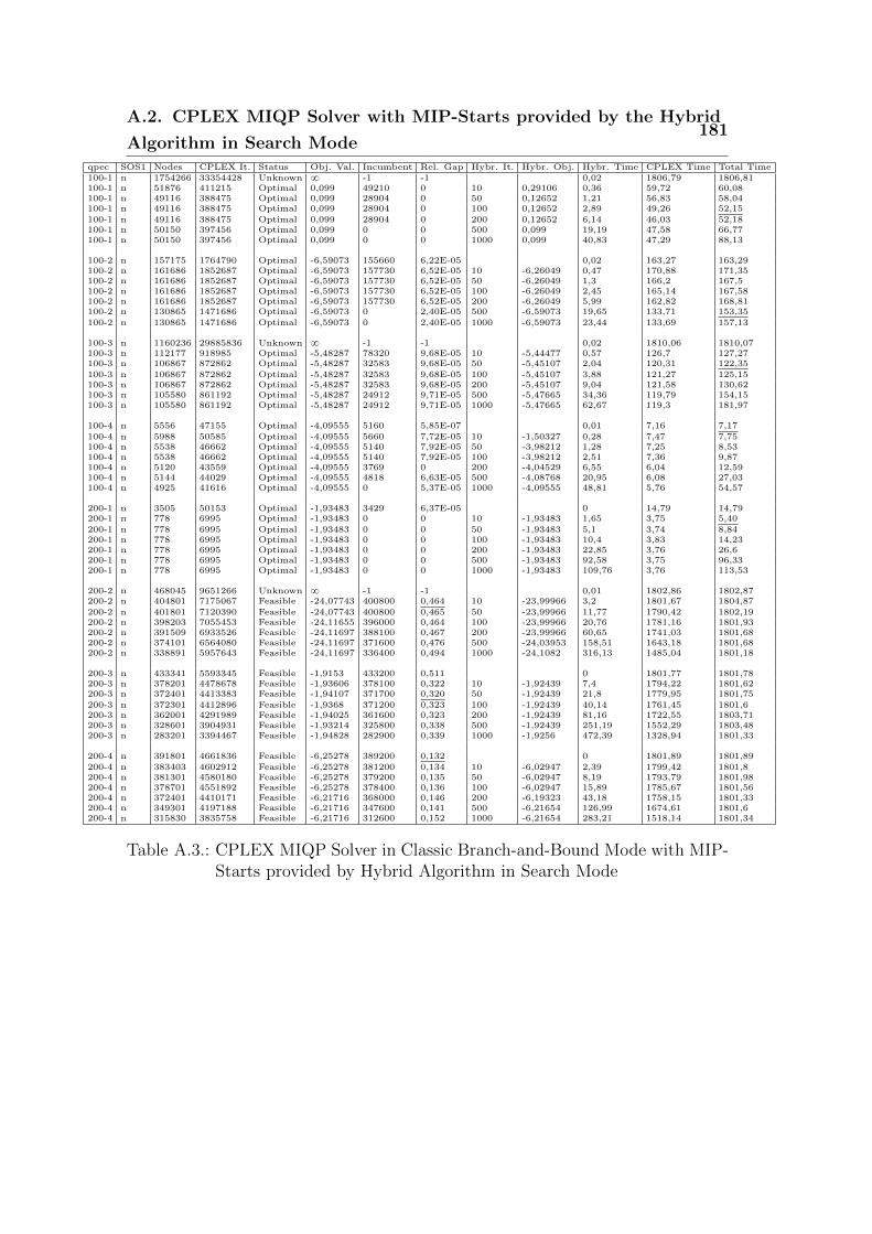
A.2. CPLEX MIQP Solver with MIP-Starts provided by the Hybrid
Algorithm in Search Mode181
qpec SOS1 Nodes CPLEX It. Status Obj. Val. Incumbent Rel. Gap Hybr. It. Hybr. Obj. Hybr. Time CPLEX Time Total Time100-1 n 1754266 33354428 Unknown 8 -1 -1 0,02 1806,79 1806,81100-1 n 51876 411215 Optimal 0,099 49210 0 10 0,29106 0,36 59,72 60,08100-1 n 49116 388475 Optimal 0,099 28904 0 50 0,12652 1,21 56,83 58,04100-1 n 49116 388475 Optimal 0,099 28904 0 100 0,12652 2,89 49,26 52,15
100-1 n 49116 388475 Optimal 0,099 28904 0 200 0,12652 6,14 46,03 52,18100-1 n 50150 397456 Optimal 0,099 0 0 500 0,099 19,19 47,58 66,77100-1 n 50150 397456 Optimal 0,099 0 0 1000 0,099 40,83 47,29 88,13
100-2 n 157175 1764790 Optimal -6,59073 155660 6,22E-05 0,02 163,27 163,29100-2 n 161686 1852687 Optimal -6,59073 157730 6,52E-05 10 -6,26049 0,47 170,88 171,35100-2 n 161686 1852687 Optimal -6,59073 157730 6,52E-05 50 -6,26049 1,3 166,2 167,5100-2 n 161686 1852687 Optimal -6,59073 157730 6,52E-05 100 -6,26049 2,45 165,14 167,58100-2 n 161686 1852687 Optimal -6,59073 157730 6,52E-05 200 -6,26049 5,99 162,82 168,81100-2 n 130865 1471686 Optimal -6,59073 0 2,40E-05 500 -6,59073 19,65 133,71 153,35
100-2 n 130865 1471686 Optimal -6,59073 0 2,40E-05 1000 -6,59073 23,44 133,69 157,13
100-3 n 1160236 29885836 Unknown 8 -1 -1 0,02 1810,06 1810,07100-3 n 112177 918985 Optimal -5,48287 78320 9,68E-05 10 -5,44477 0,57 126,7 127,27100-3 n 106867 872862 Optimal -5,48287 32583 9,68E-05 50 -5,45107 2,04 120,31 122,35
100-3 n 106867 872862 Optimal -5,48287 32583 9,68E-05 100 -5,45107 3,88 121,27 125,15100-3 n 106867 872862 Optimal -5,48287 32583 9,68E-05 200 -5,45107 9,04 121,58 130,62100-3 n 105580 861192 Optimal -5,48287 24912 9,71E-05 500 -5,47665 34,36 119,79 154,15100-3 n 105580 861192 Optimal -5,48287 24912 9,71E-05 1000 -5,47665 62,67 119,3 181,97
100-4 n 5556 47155 Optimal -4,09555 5160 5,85E-07 0,01 7,16 7,17
100-4 n 5988 50585 Optimal -4,09555 5660 7,72E-05 10 -1,50327 0,28 7,47 7,75100-4 n 5538 46662 Optimal -4,09555 5140 7,92E-05 50 -3,98212 1,28 7,25 8,53100-4 n 5538 46662 Optimal -4,09555 5140 7,92E-05 100 -3,98212 2,51 7,36 9,87100-4 n 5120 43559 Optimal -4,09555 3769 0 200 -4,04529 6,55 6,04 12,59100-4 n 5144 44029 Optimal -4,09555 4818 6,63E-05 500 -4,08768 20,95 6,08 27,03100-4 n 4925 41616 Optimal -4,09555 0 5,37E-05 1000 -4,09555 48,81 5,76 54,57
200-1 n 3505 50153 Optimal -1,93483 3429 6,37E-05 0 14,79 14,79200-1 n 778 6995 Optimal -1,93483 0 0 10 -1,93483 1,65 3,75 5,40
200-1 n 778 6995 Optimal -1,93483 0 0 50 -1,93483 5,1 3,74 8,84200-1 n 778 6995 Optimal -1,93483 0 0 100 -1,93483 10,4 3,83 14,23200-1 n 778 6995 Optimal -1,93483 0 0 200 -1,93483 22,85 3,76 26,6200-1 n 778 6995 Optimal -1,93483 0 0 500 -1,93483 92,58 3,75 96,33200-1 n 778 6995 Optimal -1,93483 0 0 1000 -1,93483 109,76 3,76 113,53
200-2 n 468045 9651266 Unknown 8 -1 -1 0,01 1802,86 1802,87200-2 n 404801 7175067 Feasible -24,07743 400800 0,464 10 -23,99966 3,2 1801,67 1804,87
200-2 n 401801 7120390 Feasible -24,07743 400800 0,465 50 -23,99966 11,77 1790,42 1802,19200-2 n 398203 7055453 Feasible -24,11655 396000 0,464 100 -23,99966 20,76 1781,16 1801,93200-2 n 391509 6933526 Feasible -24,11697 388100 0,467 200 -23,99966 60,65 1741,03 1801,68200-2 n 374101 6564080 Feasible -24,11697 371600 0,476 500 -24,03953 158,51 1643,18 1801,68200-2 n 338891 5957643 Feasible -24,11697 336400 0,494 1000 -24,1082 316,13 1485,04 1801,18
200-3 n 433341 5593345 Feasible -1,9153 433200 0,511 0 1801,77 1801,78200-3 n 378201 4478678 Feasible -1,93606 378100 0,322 10 -1,92439 7,4 1794,22 1801,62200-3 n 372401 4413383 Feasible -1,94107 371700 0,320 50 -1,92439 21,8 1779,95 1801,75
200-3 n 372301 4412896 Feasible -1,9368 371200 0,323 100 -1,92439 40,14 1761,45 1801,6200-3 n 362001 4291989 Feasible -1,94025 361600 0,323 200 -1,92439 81,16 1722,55 1803,71200-3 n 328601 3904931 Feasible -1,93214 325800 0,338 500 -1,92439 251,19 1552,29 1803,48200-3 n 283201 3394467 Feasible -1,94828 282900 0,339 1000 -1,9256 472,39 1328,94 1801,33
200-4 n 391801 4661836 Feasible -6,25278 389200 0,132 0 1801,89 1801,89
200-4 n 383403 4602912 Feasible -6,25278 381200 0,134 10 -6,02947 2,39 1799,42 1801,8200-4 n 381301 4580180 Feasible -6,25278 379200 0,135 50 -6,02947 8,19 1793,79 1801,98200-4 n 378701 4551892 Feasible -6,25278 378400 0,136 100 -6,02947 15,89 1785,67 1801,56200-4 n 372401 4410171 Feasible -6,21716 368000 0,146 200 -6,19323 43,18 1758,15 1801,33200-4 n 349301 4197188 Feasible -6,21716 347600 0,141 500 -6,21654 126,99 1674,61 1801,6200-4 n 315830 3835758 Feasible -6,21716 312600 0,152 1000 -6,21654 283,21 1518,14 1801,34
Table A.3.: CPLEX MIQP Solver in Classic Branch-and-Bound Mode with MIP-Starts provided by Hybrid Algorithm in Search Mode

A.2. CPLEX MIQP Solver with MIP-Starts provided by the Hybrid
Algorithm in Search Mode182
qpec SOS1 Nodes CPLEX It. Status Obj. Val. Incumbent Rel. Gap Hybr. It. Hybr. Obj. Hybr. Time CPLEX Time Total Time100-1 y 74846 427291 Optimal 0,099 46017 3,21E-05 0,01 69,41 69,42100-1 y 59268 338731 Optimal 0,099 10374 1,49E-05 10 0,29106 0,31 50,68 50,99100-1 y 61114 351131 Optimal 0,099 56073 0 50 0,12652 1,23 49,39 50,62100-1 y 61114 351131 Optimal 0,099 56073 0 100 0,12652 2,7 47,32 50,02100-1 y 61114 351131 Optimal 0,099 56073 0 200 0,12652 5,95 47,11 53,06100-1 y 60005 344718 Optimal 0,099 0 0 500 0,099 19,07 44,89 63,95100-1 y 60005 344718 Optimal 0,099 0 0 1000 0,099 40,71 44,76 85,47100-1 n 1210550 35496987 Unknown 8 -1 -1 0,02 1804,04 1804,06100-1 n 38664 295276 Optimal 0,099 37650 0 10 0,29106 0,36 44,8 45,17100-1 n 39649 308248 Optimal 0,099 26580 0 50 0,12652 1,21 41,08 42,29100-1 n 39649 308248 Optimal 0,099 26580 0 100 0,12652 2,89 38,6 41,49
100-1 n 39649 308248 Optimal 0,099 26580 0 200 0,12652 6,14 37,01 43,15100-1 n 38928 299587 Optimal 0,099 0 7,59E-07 500 0,099 19,19 37,92 57,1100-1 n 38928 299587 Optimal 0,099 0 7,59E-07 1000 0,099 40,83 35,83 76,66
100-2 y 258771 2206896 Optimal -6,59073 252919 9,44E-05 0,02 246,07 246,08100-2 y 249180 2085497 Optimal -6,59073 248271 7,47E-05 10 -6,26049 0,47 238,79 239,26100-2 y 249180 2085497 Optimal -6,59073 248271 7,47E-05 50 -6,26049 1,25 225,77 227,02100-2 y 249180 2085497 Optimal -6,59073 248271 7,47E-05 100 -6,26049 2,43 229,28 231,71100-2 y 249180 2085497 Optimal -6,59073 248271 7,47E-05 200 -6,26049 5,95 223,82 229,77100-2 y 264106 2289819 Optimal -6,59073 0 8,56E-05 500 -6,59073 19,67 235,8 255,47100-2 y 264106 2289819 Optimal -6,59073 0 8,56E-05 1000 -6,59073 23,59 241,58 265,18100-2 n 281878 2936708 Optimal -6,59073 281770 9,55E-05 0,02 293,37 293,4100-2 n 132563 1367985 Optimal -6,59073 60080 8,94E-05 10 -6,26049 0,47 138,11 138,58100-2 n 132563 1367985 Optimal -6,59073 60080 8,94E-05 50 -6,26049 1,3 132,76 134,06
100-2 n 132563 1367985 Optimal -6,59073 60080 8,94E-05 100 -6,26049 2,45 133,57 136,02100-2 n 132563 1367985 Optimal -6,59073 60080 8,94E-05 200 -6,26049 5,99 132,13 138,12100-2 n 129228 1329031 Optimal -6,59073 0 7,49E-05 500 -6,59073 19,65 127,91 147,56100-2 n 129228 1329031 Optimal -6,59073 0 7,49E-05 1000 -6,59073 23,44 127,68 151,12
100-3 y 915930 5286060 Optimal -5,48287 818401 9,89E-05 0,02 1028,5 1028,52100-3 y 170253 1023256 Optimal -5,48287 155036 9,99E-05 10 -5,44477 0,56 200,88 201,44100-3 y 201287 1146330 Optimal -5,48287 194578 9,79E-05 50 -5,45107 2,05 231,72 233,77100-3 y 201287 1146330 Optimal -5,48287 194578 9,79E-05 100 -5,45107 3,88 233,36 237,24100-3 y 201287 1146330 Optimal -5,48287 194578 9,79E-05 200 -5,45107 8,93 233,38 242,31100-3 y 167877 1001409 Optimal -5,48287 157253 9,98E-05 500 -5,47665 34,62 189,99 224,61100-3 y 167877 1001409 Optimal -5,48287 157253 9,98E-05 1000 -5,47665 62,47 191,7 254,17100-3 n 109213 823213 Optimal -5,48287 88377 9,95E-05 0,02 129,6 129,62
100-3 n 112500 858696 Optimal -5,48287 410 8,29E-05 10 -5,44477 0,57 131,95 132,52100-3 n 115696 873092 Optimal -5,48287 66870 9,66E-05 50 -5,45107 2,04 134,22 136,27100-3 n 115696 873092 Optimal -5,48287 66870 9,66E-05 100 -5,45107 3,88 134,54 138,42100-3 n 115696 873092 Optimal -5,48287 66870 9,66E-05 200 -5,45107 9,04 134,57 143,61100-3 n 113692 866933 Optimal -5,48287 105250 9,41E-05 500 -5,47665 34,36 131,33 165,7100-3 n 113692 866933 Optimal -5,48287 105250 9,41E-05 1000 -5,47665 62,67 133,55 196,22
100-4 y 4200 29026 Optimal -4,09555 2954 1,74E-05 0,01 5,83 5,84100-4 y 6319 38162 Optimal -4,09555 6200 0 10 -1,50327 0,27 10,58 10,85100-4 y 4435 29804 Optimal -4,09555 4383 7,90E-05 50 -3,98212 1,29 7,02 8,3100-4 y 4435 29804 Optimal -4,09555 4383 7,90E-05 100 -3,98212 2,42 6,95 9,37100-4 y 4433 29817 Optimal -4,09555 4367 4,96E-05 200 -4,04529 6,42 7,16 13,58100-4 y 4563 30683 Optimal -4,09555 3395 8,44E-06 500 -4,08768 21,06 6,26 27,32100-4 y 4569 30582 Optimal -4,09555 0 7,90E-05 1000 -4,09555 48,96 5,5 54,46100-4 n 3321 26961 Optimal -4,09555 1464 6,06E-05 0,01 4,71 4,72
100-4 n 3355 27497 Optimal -4,09555 3230 0 10 -1,50327 0,28 5,09 5,37100-4 n 3497 27939 Optimal -4,09555 2555 8,39E-05 50 -3,98212 1,28 4,75 6,03100-4 n 3497 27939 Optimal -4,09555 2555 8,39E-05 100 -3,98212 2,51 4,84 7,35100-4 n 3641 28780 Optimal -4,09555 3417 0 200 -4,04529 6,55 5,1 11,65100-4 n 3386 27570 Optimal -4,09555 2750 0 500 -4,08768 20,95 4,32 25,27100-4 n 3371 27731 Optimal -4,09555 0 9,14E-05 1000 -4,09555 48,81 4,16 52,97
Table A.4.: CPLEX MIQP Solver in Dynamic Search Mode with MIP-Starts pro-vided by the Hybrid Algorithm in Search Mode

A.2. CPLEX MIQP Solver with MIP-Starts provided by the Hybrid
Algorithm in Search Mode183
qpec SOS1 Nodes CPLEX It. Status Obj. Val. Incumbent Rel. Gap Hybr. It. Hybr. Obj. Hybr. Time CPLEX Time Total Time200-1 y 92176 717360 Optimal -1,93483 2821 9,96E-05 0 257,08 257,08200-1 y 567 4185 Optimal -1,93483 0 0 10 -1,93483 1,64 2,35 3,99
200-1 y 567 4185 Optimal -1,93483 0 0 50 -1,93483 5,09 2,32 7,41200-1 y 567 4185 Optimal -1,93483 0 0 100 -1,93483 10,39 2,31 12,7200-1 y 567 4185 Optimal -1,93483 0 0 200 -1,93483 22,81 2,34 25,15200-1 y 567 4185 Optimal -1,93483 0 0 500 -1,93483 92,97 2,31 95,28200-1 y 567 4185 Optimal -1,93483 0 0 1000 -1,93483 109,35 2,34 111,69200-1 n 435230 3981484 Optimal -1,93516 430157 1,00E-04 0 1064,59 1064,6200-1 n 1067 9430 Optimal -1,93509 1047 0 10 -1,93483 1,65 6,47 8,12200-1 n 1067 9430 Optimal -1,93509 1047 0 50 -1,93483 5,1 6,47 11,57200-1 n 1067 9430 Optimal -1,93509 1047 0 100 -1,93483 10,4 6,39 16,79200-1 n 1067 9430 Optimal -1,93509 1047 0 200 -1,93483 22,85 6,42 29,27200-1 n 1067 9430 Optimal -1,93509 1047 0 500 -1,93483 92,58 6,42 98,99200-1 n 1067 9430 Optimal -1,93509 1047 0 1000 -1,93483 109,76 6,42 116,18
200-2 y 245001 5187562 Feasible -22,6029 80886 0,819 0 1800,83 1800,83200-2 y 252801 5413271 Feasible -23,99966 0 0,552 10 -23,99966 3,22 1797,34 1800,56200-2 y 251501 5386953 Feasible -23,99966 0 0,553 50 -23,99966 11,74 1789,18 1800,92200-2 y 251201 5380277 Feasible -23,99966 0 0,553 100 -23,99966 20,87 1779,84 1800,71200-2 y 244541 5244856 Feasible -23,99966 0 0,558 200 -23,99966 60,57 1740,11 1800,68200-2 y 230846 4922057 Feasible -24,03953 0 0,564 500 -24,03953 158,81 1641,9 1800,71200-2 y 209101 4475846 Feasible -24,1082 0 0,574 1000 -24,1082 315,87 1484,84 1800,71200-2 n 351332 9321787 Unknown 8 -1 -1 0,01 1801,22 1801,22200-2 n 436120 7057266 Feasible -24,07743 432600 0,47 10 -23,99966 3,2 1798,2 1801,4200-2 n 443201 7171227 Feasible -24,07743 438700 0,467 50 -23,99966 11,77 1789,84 1801,61200-2 n 442101 7153787 Feasible -24,11697 441500 0,464885198 100 -23,99966 20,76 1780,67 1801,44
200-2 n 428401 6932466 Feasible -24,11697 426000 0,47 200 -23,99966 60,65 1740,78 1801,43200-2 n 408301 6645455 Feasible -24,07743 406400 0,475 500 -24,03953 158,51 1642,81 1801,31200-2 n 374506 6012051 Feasible -24,11697 368800 0,487 1000 -24,1082 316,13 1484,95 1801,08
200-3 y 240714 2809101 Feasible -1,88717 177458 0,751 0 1800,96 1800,96200-3 y 251001 2960089 Feasible -1,92439 0 0,468 10 -1,92439 7,44 1794,12 1801,56200-3 y 249201 2939027 Feasible -1,92439 0 0,469 50 -1,92439 21,76 1780,76 1802,52200-3 y 247201 2915647 Feasible -1,92439 0 0,47 100 -1,92439 40,21 1760,7 1800,9200-3 y 243601 2872961 Feasible -1,92439 0 0,471 200 -1,92439 81,25 1721,67 1802,93200-3 y 219001 2583868 Feasible -1,92439 0 0,483 500 -1,92439 251,26 1549,66 1800,91200-3 y 185597 2213609 Feasible -1,9256 0 0,498 1000 -1,9256 473,16 1327,28 1800,44200-3 n 433501 5381262 Feasible -1,95341 432800 0,474 0 1801,59 1801,59200-3 n 419001 4841221 Feasible -1,9522 418800 0,332371782 10 -1,92439 7,4 1793,78 1801,18
200-3 n 414801 4791903 Feasible -1,93954 414000 0,342 50 -1,92439 21,8 1779,5 1801,3200-3 n 414001 4782604 Feasible -1,93573 413300 0,345 100 -1,92439 40,14 1760,93 1801,08200-3 n 400601 4627155 Feasible -1,94234 399400 0,343 200 -1,92439 81,16 1720,2 1801,36200-3 n 364401 4205447 Feasible -1,93682 364000 0,356 500 -1,92439 251,19 1550,36 1801,56200-3 n 310701 3637192 Feasible -1,94304 310400 0,366 1000 -1,9256 472,39 1328,76 1801,16
200-4 y 288301 3329273 Feasible -6,22036 228583 0,15 0,01 1800,89 1800,9200-4 y 295401 3455881 Feasible -6,16877 233848 0,164 10 -6,02947 2,42 1798,65 1801,07200-4 y 295401 3455881 Feasible -6,16877 233848 0,164 50 -6,02947 8,18 1793 1801,18200-4 y 293001 3433130 Feasible -6,16877 233848 0,165 100 -6,02947 15,91 1785,41 1801,33200-4 y 293501 3329220 Feasible -6,19323 0 0,153 200 -6,19323 43,63 1757,48 1801,11200-4 y 276101 3155215 Feasible -6,21654 0 0,15 500 -6,21654 126,17 1674,92 1801,1200-4 y 246701 2881877 Feasible -6,21654 0 0,163 1000 -6,21654 298,6 1501,96 1800,56200-4 n 402701 4276686 Feasible -6,25278 397200 0,054558096 0 1801,61 1801,61
200-4 n 396101 4315258 Feasible -6,25278 386000 0,071 10 -6,02947 2,39 1799,12 1801,51200-4 n 409558 4441969 Feasible -6,25278 390800 0,067 50 -6,02947 8,19 1793,22 1801,4200-4 n 395301 4308083 Feasible -6,25278 381200 0,071 100 -6,02947 15,89 1785,72 1801,61200-4 n 391310 4194896 Feasible -6,25278 376700 0,059 200 -6,19323 43,18 1758,19 1801,37200-4 n 361601 3923367 Feasible -6,25278 356800 0,069 500 -6,21654 126,99 1674,41 1801,4200-4 n 331501 3644428 Feasible -6,21716 324300 0,086 1000 -6,21654 283,21 1517,96 1801,17
Table A.5.: CPLEX MIQP Solver in Dynamic Search Mode with MIP-Starts pro-vided by the Hybrid Algorithm in Search Mode

A.3. The Hybrid Algorithm on Global Optimality 184
A.3. The Hybrid Algorithm on Global Optimality
Appending section 8.5:
The table columns are defined as follows:
• s - Problemsize, number of complemen-
tary constraints is 2s
• Ph1 It. - Iterations of the search phase
• Ph1 Obj. - Objective value after search
phase of the algorithm
• UB - Upper bound of the hybrid algo-
rithm
• LB - Lower bound of the hybrid algo-
rithm
• C. Obj. - Cplex Objective value
• C. Inc. - Cplex incumbent node
• It. - The number of iterations of the
hybrid solver
• S. Calls - Calls to the QP/LP-Solver of
the core solver
• t - Solving time of the hybrid solver
• Feas. - Whether the feasibility unit was
active
• F. Thr. - The threshold in the feasibil-
ity module (see section 5.3.1)
• M. Infeas. - Whether the BBASET
branching from a stationary point was
performed by the largest negative dual
or the most infeasibel index (see section
7.6.3)
• CASET - Whether the CASET algo-
rithm and related features were uti-
lized at all; if not then most infeasible
branching is used
• F. MIPs - The number of MIP calls in
the feasibility unit
• F. LPs - The number of LP calls in the
feasibility unit
• Dual Bnds. - The number of Lagrange
dual bounds that have been calculated
• Cuts - The total number of disjunctive
cuts that have been generated
• LPs - LP calls in the variable bound
constraint generation (alg. 18)
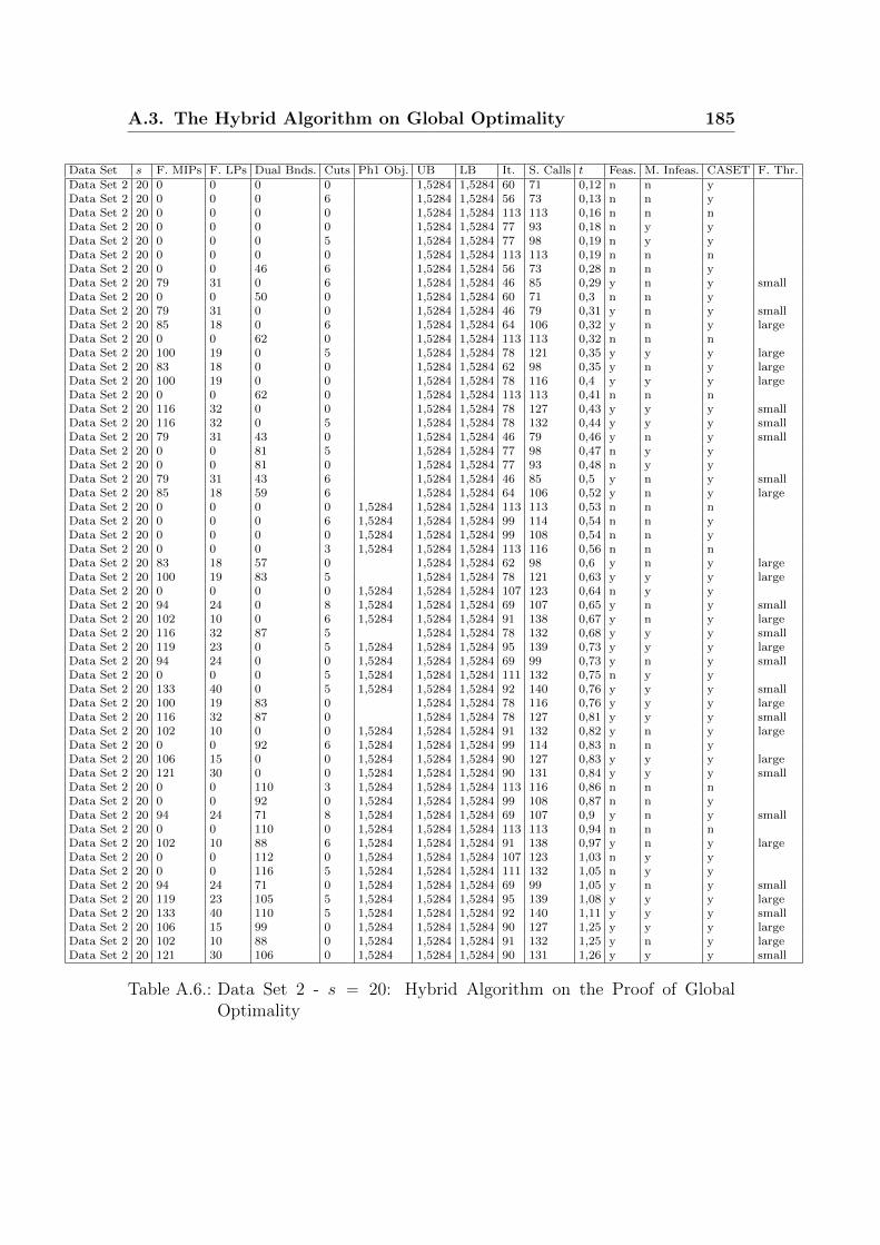
A.3. The Hybrid Algorithm on Global Optimality 185
Data Set s F. MIPs F. LPs Dual Bnds. Cuts Ph1 Obj. UB LB It. S. Calls t Feas. M. Infeas. CASET F. Thr.Data Set 2 20 0 0 0 0 1,5284 1,5284 60 71 0,12 n n yData Set 2 20 0 0 0 6 1,5284 1,5284 56 73 0,13 n n yData Set 2 20 0 0 0 0 1,5284 1,5284 113 113 0,16 n n nData Set 2 20 0 0 0 0 1,5284 1,5284 77 93 0,18 n y yData Set 2 20 0 0 0 5 1,5284 1,5284 77 98 0,19 n y yData Set 2 20 0 0 0 0 1,5284 1,5284 113 113 0,19 n n nData Set 2 20 0 0 46 6 1,5284 1,5284 56 73 0,28 n n yData Set 2 20 79 31 0 6 1,5284 1,5284 46 85 0,29 y n y smallData Set 2 20 0 0 50 0 1,5284 1,5284 60 71 0,3 n n yData Set 2 20 79 31 0 0 1,5284 1,5284 46 79 0,31 y n y smallData Set 2 20 85 18 0 6 1,5284 1,5284 64 106 0,32 y n y largeData Set 2 20 0 0 62 0 1,5284 1,5284 113 113 0,32 n n nData Set 2 20 100 19 0 5 1,5284 1,5284 78 121 0,35 y y y largeData Set 2 20 83 18 0 0 1,5284 1,5284 62 98 0,35 y n y largeData Set 2 20 100 19 0 0 1,5284 1,5284 78 116 0,4 y y y largeData Set 2 20 0 0 62 0 1,5284 1,5284 113 113 0,41 n n nData Set 2 20 116 32 0 0 1,5284 1,5284 78 127 0,43 y y y smallData Set 2 20 116 32 0 5 1,5284 1,5284 78 132 0,44 y y y smallData Set 2 20 79 31 43 0 1,5284 1,5284 46 79 0,46 y n y smallData Set 2 20 0 0 81 5 1,5284 1,5284 77 98 0,47 n y yData Set 2 20 0 0 81 0 1,5284 1,5284 77 93 0,48 n y yData Set 2 20 79 31 43 6 1,5284 1,5284 46 85 0,5 y n y smallData Set 2 20 85 18 59 6 1,5284 1,5284 64 106 0,52 y n y largeData Set 2 20 0 0 0 0 1,5284 1,5284 1,5284 113 113 0,53 n n nData Set 2 20 0 0 0 6 1,5284 1,5284 1,5284 99 114 0,54 n n yData Set 2 20 0 0 0 0 1,5284 1,5284 1,5284 99 108 0,54 n n yData Set 2 20 0 0 0 3 1,5284 1,5284 1,5284 113 116 0,56 n n nData Set 2 20 83 18 57 0 1,5284 1,5284 62 98 0,6 y n y largeData Set 2 20 100 19 83 5 1,5284 1,5284 78 121 0,63 y y y largeData Set 2 20 0 0 0 0 1,5284 1,5284 1,5284 107 123 0,64 n y yData Set 2 20 94 24 0 8 1,5284 1,5284 1,5284 69 107 0,65 y n y smallData Set 2 20 102 10 0 6 1,5284 1,5284 1,5284 91 138 0,67 y n y largeData Set 2 20 116 32 87 5 1,5284 1,5284 78 132 0,68 y y y smallData Set 2 20 119 23 0 5 1,5284 1,5284 1,5284 95 139 0,73 y y y largeData Set 2 20 94 24 0 0 1,5284 1,5284 1,5284 69 99 0,73 y n y smallData Set 2 20 0 0 0 5 1,5284 1,5284 1,5284 111 132 0,75 n y yData Set 2 20 133 40 0 5 1,5284 1,5284 1,5284 92 140 0,76 y y y smallData Set 2 20 100 19 83 0 1,5284 1,5284 78 116 0,76 y y y largeData Set 2 20 116 32 87 0 1,5284 1,5284 78 127 0,81 y y y smallData Set 2 20 102 10 0 0 1,5284 1,5284 1,5284 91 132 0,82 y n y largeData Set 2 20 0 0 92 6 1,5284 1,5284 1,5284 99 114 0,83 n n yData Set 2 20 106 15 0 0 1,5284 1,5284 1,5284 90 127 0,83 y y y largeData Set 2 20 121 30 0 0 1,5284 1,5284 1,5284 90 131 0,84 y y y smallData Set 2 20 0 0 110 3 1,5284 1,5284 1,5284 113 116 0,86 n n nData Set 2 20 0 0 92 0 1,5284 1,5284 1,5284 99 108 0,87 n n yData Set 2 20 94 24 71 8 1,5284 1,5284 1,5284 69 107 0,9 y n y smallData Set 2 20 0 0 110 0 1,5284 1,5284 1,5284 113 113 0,94 n n nData Set 2 20 102 10 88 6 1,5284 1,5284 1,5284 91 138 0,97 y n y largeData Set 2 20 0 0 112 0 1,5284 1,5284 1,5284 107 123 1,03 n y yData Set 2 20 0 0 116 5 1,5284 1,5284 1,5284 111 132 1,05 n y yData Set 2 20 94 24 71 0 1,5284 1,5284 1,5284 69 99 1,05 y n y smallData Set 2 20 119 23 105 5 1,5284 1,5284 1,5284 95 139 1,08 y y y largeData Set 2 20 133 40 110 5 1,5284 1,5284 1,5284 92 140 1,11 y y y smallData Set 2 20 106 15 99 0 1,5284 1,5284 1,5284 90 127 1,25 y y y largeData Set 2 20 102 10 88 0 1,5284 1,5284 1,5284 91 132 1,25 y n y largeData Set 2 20 121 30 106 0 1,5284 1,5284 1,5284 90 131 1,26 y y y small
Table A.6.: Data Set 2 - s “ 20: Hybrid Algorithm on the Proof of GlobalOptimality
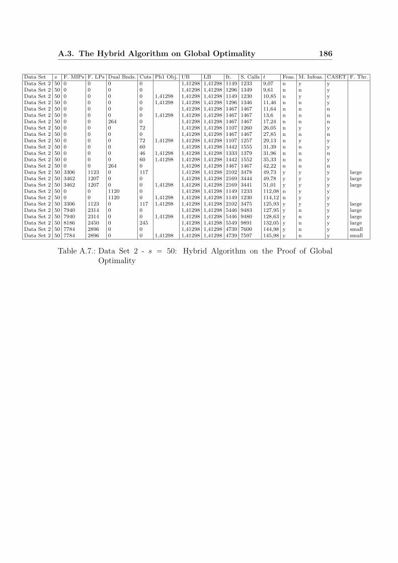
A.3. The Hybrid Algorithm on Global Optimality 186
Data Set s F. MIPs F. LPs Dual Bnds. Cuts Ph1 Obj. UB LB It. S. Calls t Feas. M. Infeas. CASET F. Thr.Data Set 2 50 0 0 0 0 1,41298 1,41298 1149 1233 9,07 n y yData Set 2 50 0 0 0 0 1,41298 1,41298 1296 1349 9,61 n n yData Set 2 50 0 0 0 0 1,41298 1,41298 1,41298 1149 1230 10,85 n y yData Set 2 50 0 0 0 0 1,41298 1,41298 1,41298 1296 1346 11,46 n n yData Set 2 50 0 0 0 0 1,41298 1,41298 1467 1467 11,64 n n nData Set 2 50 0 0 0 0 1,41298 1,41298 1,41298 1467 1467 13,6 n n nData Set 2 50 0 0 264 0 1,41298 1,41298 1467 1467 17,24 n n nData Set 2 50 0 0 0 72 1,41298 1,41298 1107 1260 26,05 n y yData Set 2 50 0 0 0 0 1,41298 1,41298 1467 1467 27,85 n n nData Set 2 50 0 0 0 72 1,41298 1,41298 1,41298 1107 1257 29,13 n y yData Set 2 50 0 0 0 60 1,41298 1,41298 1442 1555 31,39 n n yData Set 2 50 0 0 0 46 1,41298 1,41298 1,41298 1333 1379 31,96 n n nData Set 2 50 0 0 0 60 1,41298 1,41298 1,41298 1442 1552 35,33 n n yData Set 2 50 0 0 264 0 1,41298 1,41298 1467 1467 42,22 n n nData Set 2 50 3306 1123 0 117 1,41298 1,41298 2102 3478 49,73 y y y largeData Set 2 50 3462 1207 0 0 1,41298 1,41298 2169 3444 49,78 y y y largeData Set 2 50 3462 1207 0 0 1,41298 1,41298 1,41298 2169 3441 51,01 y y y largeData Set 2 50 0 0 1120 0 1,41298 1,41298 1149 1233 112,08 n y yData Set 2 50 0 0 1120 0 1,41298 1,41298 1,41298 1149 1230 114,12 n y yData Set 2 50 3306 1123 0 117 1,41298 1,41298 1,41298 2102 3475 125,93 y y y largeData Set 2 50 7940 2314 0 0 1,41298 1,41298 5446 9483 127,95 y n y largeData Set 2 50 7940 2314 0 0 1,41298 1,41298 1,41298 5446 9480 128,63 y n y largeData Set 2 50 8186 2450 0 245 1,41298 1,41298 5549 9891 132,05 y n y largeData Set 2 50 7784 2896 0 0 1,41298 1,41298 4739 7600 144,98 y n y smallData Set 2 50 7784 2896 0 0 1,41298 1,41298 1,41298 4739 7597 145,98 y n y small
Table A.7.: Data Set 2 - s “ 50: Hybrid Algorithm on the Proof of GlobalOptimality

A.3. The Hybrid Algorithm on Global Optimality 187
Data Set s F. MIPs F. LPs Dual Bnds. Cuts Ph1 Obj. UB LB It. S. Calls t Feas. M. Infeas. CASET F. Thr.Data Set 3 30 0 0 1 0 0,88696 0,88696 41 41 0,06 n n nData Set 3 30 0 0 0 0 0,88696 0,88696 41 41 0,06 n n nData Set 3 30 0 0 0 0 0,88696 0,88696 41 41 0,06 n n nData Set 3 30 0 0 1 0 0,88696 0,88696 41 41 0,07 n n nData Set 3 30 0 0 0 0 0,88696 0,88696 21 31 0,08 n n yData Set 3 30 0 0 0 0 0,88696 0,88696 10 21 0,09 n y yData Set 3 30 0 0 0 0 0,88696 0,88696 21 31 0,1 n n yData Set 3 30 10 0 0 0 0,88696 0,88696 10 21 0,11 y y y smallData Set 3 30 0 0 0 1 0,88696 0,88696 10 22 0,12 n y yData Set 3 30 10 0 0 0 0,88696 0,88696 10 21 0,12 y y y largeData Set 3 30 10 0 0 1 0,88696 0,88696 10 22 0,14 y y y smallData Set 3 30 10 0 0 1 0,88696 0,88696 10 22 0,14 y y y largeData Set 3 30 25 4 0 0 0,88696 0,88696 21 31 0,15 y n y largeData Set 3 30 25 4 0 0 0,88696 0,88696 21 31 0,16 y n y largeData Set 3 30 0 0 20 0 0,88696 0,88696 10 21 0,19 n y yData Set 3 30 0 0 20 1 0,88696 0,88696 10 22 0,2 n y yData Set 3 30 10 0 20 0 0,88696 0,88696 10 21 0,21 y y y smallData Set 3 30 39 17 0 0 0,88696 0,88696 18 40 0,22 y n y smallData Set 3 30 10 0 20 1 0,88696 0,88696 10 22 0,23 y y y smallData Set 3 30 10 0 20 1 0,88696 0,88696 10 22 0,23 y y y largeData Set 3 30 39 17 0 0 0,88696 0,88696 18 40 0,23 y n y smallData Set 3 30 10 0 20 0 0,88696 0,88696 10 21 0,23 y y y largeData Set 3 30 0 0 32 0 0,88696 0,88696 21 31 0,24 n n yData Set 3 30 0 0 32 0 0,88696 0,88696 21 31 0,26 n n yData Set 3 30 25 4 32 0 0,88696 0,88696 21 31 0,31 y n y largeData Set 3 30 39 17 29 0 0,88696 0,88696 18 40 0,35 y n y smallData Set 3 30 25 4 32 0 0,88696 0,88696 21 31 0,38 y n y largeData Set 3 30 39 17 29 0 0,88696 0,88696 18 40 0,4 y n y smallData Set 3 30 0 0 0 1 0,88696 0,88696 0,88696 47 48 0,57 n n nData Set 3 30 0 0 0 0 0,88696 0,88696 0,88696 41 41 0,58 n n nData Set 3 30 0 0 0 2 0,88696 0,88696 0,88696 10 19 0,59 n y yData Set 3 30 0 0 0 1 0,88696 0,88696 0,88696 21 28 0,6 n n yData Set 3 30 0 0 0 0 0,88696 0,88696 0,88696 10 17 0,6 n y yData Set 3 30 0 0 0 0 0,88696 0,88696 0,88696 21 27 0,61 n n yData Set 3 30 10 0 0 2 0,88696 0,88696 0,88696 10 19 0,62 y y y smallData Set 3 30 10 0 0 0 0,88696 0,88696 0,88696 10 17 0,64 y y y smallData Set 3 30 10 0 0 2 0,88696 0,88696 0,88696 10 19 0,66 y y y largeData Set 3 30 0 0 20 2 0,88696 0,88696 0,88696 10 19 0,67 n y yData Set 3 30 25 4 0 1 0,88696 0,88696 0,88696 21 28 0,68 y n y largeData Set 3 30 10 0 20 2 0,88696 0,88696 0,88696 10 19 0,69 y y y smallData Set 3 30 0 0 20 0 0,88696 0,88696 0,88696 10 17 0,69 n y yData Set 3 30 10 0 0 0 0,88696 0,88696 0,88696 10 17 0,69 y y y largeData Set 3 30 39 17 0 1 0,88696 0,88696 0,88696 18 37 0,72 y n y smallData Set 3 30 10 0 20 2 0,88696 0,88696 0,88696 10 19 0,73 y y y largeData Set 3 30 10 0 20 0 0,88696 0,88696 0,88696 10 17 0,73 y y y smallData Set 3 30 25 4 0 0 0,88696 0,88696 0,88696 21 27 0,73 y n y largeData Set 3 30 0 0 32 1 0,88696 0,88696 0,88696 21 28 0,74 n n yData Set 3 30 0 0 32 0 0,88696 0,88696 0,88696 21 27 0,77 n n yData Set 3 30 39 17 0 0 0,88696 0,88696 0,88696 18 36 0,77 y n y smallData Set 3 30 10 0 20 0 0,88696 0,88696 0,88696 10 17 0,8 y y y largeData Set 3 30 0 0 46 1 0,88696 0,88696 0,88696 47 48 0,8 n n nData Set 3 30 0 0 40 0 0,88696 0,88696 0,88696 41 41 0,81 n n nData Set 3 30 25 4 32 1 0,88696 0,88696 0,88696 21 28 0,84 y n y largeData Set 3 30 39 17 29 1 0,88696 0,88696 0,88696 18 37 0,86 y n y smallData Set 3 30 25 4 32 0 0,88696 0,88696 0,88696 21 27 0,92 y n y largeData Set 3 30 39 17 29 0 0,88696 0,88696 0,88696 18 36 0,94 y n y small
Table A.8.: Data Set 3: Hybrid Algorithm on the Proof of Global Optimality
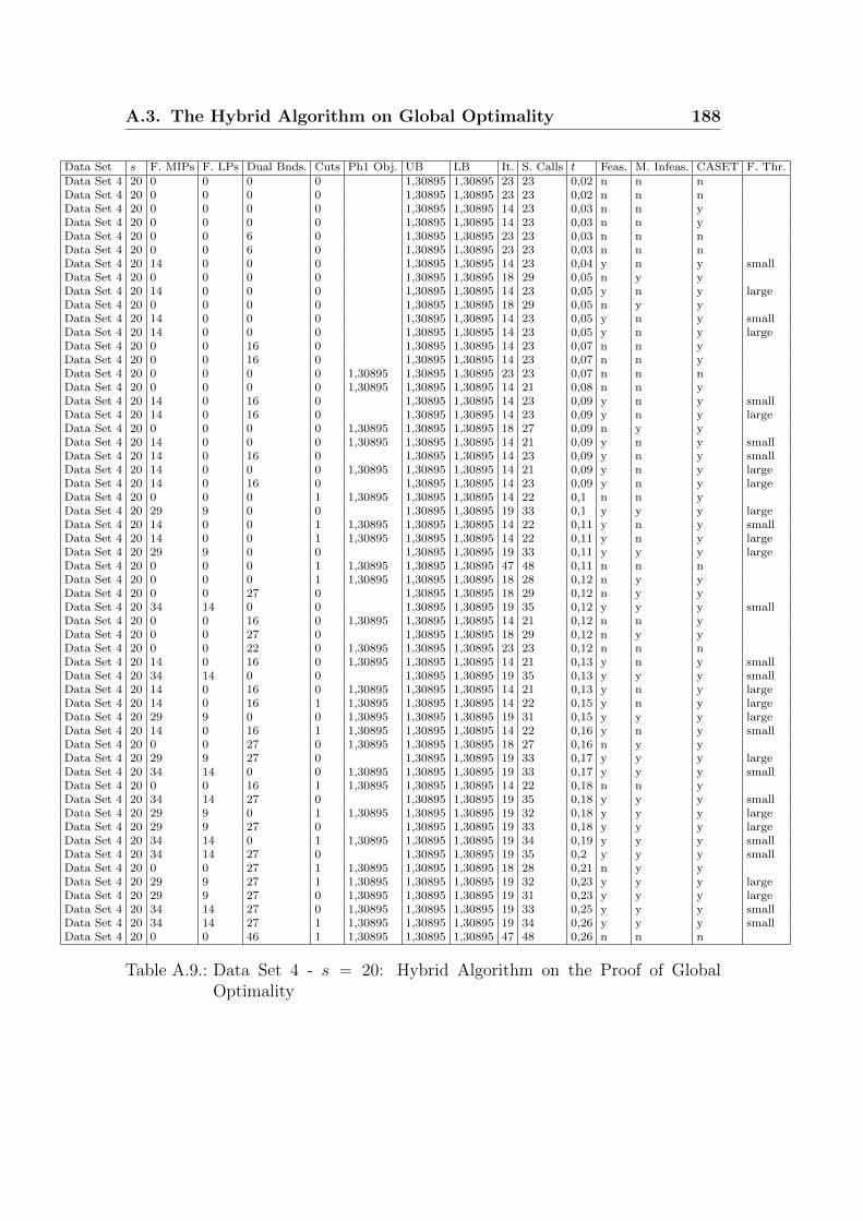
A.3. The Hybrid Algorithm on Global Optimality 188
Data Set s F. MIPs F. LPs Dual Bnds. Cuts Ph1 Obj. UB LB It. S. Calls t Feas. M. Infeas. CASET F. Thr.Data Set 4 20 0 0 0 0 1,30895 1,30895 23 23 0,02 n n nData Set 4 20 0 0 0 0 1,30895 1,30895 23 23 0,02 n n nData Set 4 20 0 0 0 0 1,30895 1,30895 14 23 0,03 n n yData Set 4 20 0 0 0 0 1,30895 1,30895 14 23 0,03 n n yData Set 4 20 0 0 6 0 1,30895 1,30895 23 23 0,03 n n nData Set 4 20 0 0 6 0 1,30895 1,30895 23 23 0,03 n n nData Set 4 20 14 0 0 0 1,30895 1,30895 14 23 0,04 y n y smallData Set 4 20 0 0 0 0 1,30895 1,30895 18 29 0,05 n y yData Set 4 20 14 0 0 0 1,30895 1,30895 14 23 0,05 y n y largeData Set 4 20 0 0 0 0 1,30895 1,30895 18 29 0,05 n y yData Set 4 20 14 0 0 0 1,30895 1,30895 14 23 0,05 y n y smallData Set 4 20 14 0 0 0 1,30895 1,30895 14 23 0,05 y n y largeData Set 4 20 0 0 16 0 1,30895 1,30895 14 23 0,07 n n yData Set 4 20 0 0 16 0 1,30895 1,30895 14 23 0,07 n n yData Set 4 20 0 0 0 0 1,30895 1,30895 1,30895 23 23 0,07 n n nData Set 4 20 0 0 0 0 1,30895 1,30895 1,30895 14 21 0,08 n n yData Set 4 20 14 0 16 0 1,30895 1,30895 14 23 0,09 y n y smallData Set 4 20 14 0 16 0 1,30895 1,30895 14 23 0,09 y n y largeData Set 4 20 0 0 0 0 1,30895 1,30895 1,30895 18 27 0,09 n y yData Set 4 20 14 0 0 0 1,30895 1,30895 1,30895 14 21 0,09 y n y smallData Set 4 20 14 0 16 0 1,30895 1,30895 14 23 0,09 y n y smallData Set 4 20 14 0 0 0 1,30895 1,30895 1,30895 14 21 0,09 y n y largeData Set 4 20 14 0 16 0 1,30895 1,30895 14 23 0,09 y n y largeData Set 4 20 0 0 0 1 1,30895 1,30895 1,30895 14 22 0,1 n n yData Set 4 20 29 9 0 0 1,30895 1,30895 19 33 0,1 y y y largeData Set 4 20 14 0 0 1 1,30895 1,30895 1,30895 14 22 0,11 y n y smallData Set 4 20 14 0 0 1 1,30895 1,30895 1,30895 14 22 0,11 y n y largeData Set 4 20 29 9 0 0 1,30895 1,30895 19 33 0,11 y y y largeData Set 4 20 0 0 0 1 1,30895 1,30895 1,30895 47 48 0,11 n n nData Set 4 20 0 0 0 1 1,30895 1,30895 1,30895 18 28 0,12 n y yData Set 4 20 0 0 27 0 1,30895 1,30895 18 29 0,12 n y yData Set 4 20 34 14 0 0 1,30895 1,30895 19 35 0,12 y y y smallData Set 4 20 0 0 16 0 1,30895 1,30895 1,30895 14 21 0,12 n n yData Set 4 20 0 0 27 0 1,30895 1,30895 18 29 0,12 n y yData Set 4 20 0 0 22 0 1,30895 1,30895 1,30895 23 23 0,12 n n nData Set 4 20 14 0 16 0 1,30895 1,30895 1,30895 14 21 0,13 y n y smallData Set 4 20 34 14 0 0 1,30895 1,30895 19 35 0,13 y y y smallData Set 4 20 14 0 16 0 1,30895 1,30895 1,30895 14 21 0,13 y n y largeData Set 4 20 14 0 16 1 1,30895 1,30895 1,30895 14 22 0,15 y n y largeData Set 4 20 29 9 0 0 1,30895 1,30895 1,30895 19 31 0,15 y y y largeData Set 4 20 14 0 16 1 1,30895 1,30895 1,30895 14 22 0,16 y n y smallData Set 4 20 0 0 27 0 1,30895 1,30895 1,30895 18 27 0,16 n y yData Set 4 20 29 9 27 0 1,30895 1,30895 19 33 0,17 y y y largeData Set 4 20 34 14 0 0 1,30895 1,30895 1,30895 19 33 0,17 y y y smallData Set 4 20 0 0 16 1 1,30895 1,30895 1,30895 14 22 0,18 n n yData Set 4 20 34 14 27 0 1,30895 1,30895 19 35 0,18 y y y smallData Set 4 20 29 9 0 1 1,30895 1,30895 1,30895 19 32 0,18 y y y largeData Set 4 20 29 9 27 0 1,30895 1,30895 19 33 0,18 y y y largeData Set 4 20 34 14 0 1 1,30895 1,30895 1,30895 19 34 0,19 y y y smallData Set 4 20 34 14 27 0 1,30895 1,30895 19 35 0,2 y y y smallData Set 4 20 0 0 27 1 1,30895 1,30895 1,30895 18 28 0,21 n y yData Set 4 20 29 9 27 1 1,30895 1,30895 1,30895 19 32 0,23 y y y largeData Set 4 20 29 9 27 0 1,30895 1,30895 1,30895 19 31 0,23 y y y largeData Set 4 20 34 14 27 0 1,30895 1,30895 1,30895 19 33 0,25 y y y smallData Set 4 20 34 14 27 1 1,30895 1,30895 1,30895 19 34 0,26 y y y smallData Set 4 20 0 0 46 1 1,30895 1,30895 1,30895 47 48 0,26 n n n
Table A.9.: Data Set 4 - s “ 20: Hybrid Algorithm on the Proof of GlobalOptimality

A.3. The Hybrid Algorithm on Global Optimality 189
Data Set s F. MIPs F. LPs Dual Bnds. Cuts Ph1 Obj. UB LB It. S. Calls t Feas. M. Infeas. CASET F. Thr.Data Set 4 40 0 0 0 0 1,18504 1,18504 131 131 0,46 n n nData Set 4 40 0 0 5 0 1,18504 1,18504 131 131 0,52 n n nData Set 4 40 0 0 0 0 1,18504 1,18504 131 131 0,54 n n nData Set 4 40 0 0 0 0 1,18523 1,18523 69 85 0,57 n n yData Set 4 40 0 0 5 0 1,18504 1,18504 131 131 0,59 n n nData Set 4 40 0 0 0 0 1,18523 1,18523 78 97 0,65 n y yData Set 4 40 0 0 0 8 1,18523 1,18523 69 93 0,7 n n yData Set 4 40 0 0 0 7 1,18523 1,18523 78 104 0,76 n y yData Set 4 40 94 13 0 0 1,18523 1,18523 79 120 1,12 y n y largeData Set 4 40 90 13 0 8 1,18523 1,18523 75 124 1,24 y n y largeData Set 4 40 132 55 0 0 1,18523 1,18523 74 124 1,39 y n y smallData Set 4 40 99 16 0 7 1,18523 1,18523 81 145 1,48 y y y largeData Set 4 40 99 16 0 0 1,18523 1,18523 81 138 1,48 y y y largeData Set 4 40 132 55 0 8 1,18523 1,18523 74 132 1,55 y n y smallData Set 4 40 163 74 0 0 1,18523 1,18523 85 123 1,66 y y y smallData Set 4 40 163 74 0 7 1,18523 1,18523 85 130 1,68 y y y smallData Set 4 40 0 0 79 8 1,18523 1,18523 69 93 1,73 n n yData Set 4 40 0 0 79 0 1,18523 1,18523 69 85 1,82 n n yData Set 4 40 0 0 96 7 1,18523 1,18523 78 104 2,07 n y yData Set 4 40 0 0 96 0 1,18523 1,18523 78 97 2,24 n y yData Set 4 40 0 0 0 2 1,18523 1,18504 1,18504 139 141 2,51 n n nData Set 4 40 0 0 0 8 1,18523 1,18523 1,18523 69 91 2,57 n n yData Set 4 40 0 0 0 0 1,18523 1,18523 1,18523 69 83 2,63 n n yData Set 4 40 0 0 0 7 1,18523 1,18523 1,18523 78 102 2,64 n y yData Set 4 40 0 0 0 0 1,18523 1,18504 1,18504 131 131 2,66 n n nData Set 4 40 90 13 93 8 1,18523 1,18523 75 124 2,76 y n y largeData Set 4 40 0 0 0 0 1,18523 1,18523 1,18523 78 95 2,78 n y yData Set 4 40 132 55 90 8 1,18523 1,18523 74 132 2,86 y n y smallData Set 4 40 132 55 90 0 1,18523 1,18523 74 124 2,96 y n y smallData Set 4 40 94 13 99 0 1,18523 1,18523 79 120 3,08 y n y largeData Set 4 40 90 13 0 8 1,18523 1,18523 1,18523 75 122 3,31 y n y largeData Set 4 40 99 16 112 7 1,18523 1,18523 81 145 3,37 y y y largeData Set 4 40 94 13 0 0 1,18523 1,18523 1,18523 79 118 3,41 y n y largeData Set 4 40 99 16 0 7 1,18523 1,18523 1,18523 81 143 3,44 y y y largeData Set 4 40 132 55 0 8 1,18523 1,18523 1,18523 74 130 3,5 y n y smallData Set 4 40 163 74 114 7 1,18523 1,18523 85 130 3,52 y y y smallData Set 4 40 132 55 0 0 1,18523 1,18523 1,18523 74 122 3,6 y n y smallData Set 4 40 99 16 113 0 1,18523 1,18523 81 138 3,6 y y y largeData Set 4 40 99 16 0 0 1,18523 1,18523 1,18523 81 136 3,64 y y y largeData Set 4 40 163 74 0 7 1,18523 1,18523 1,18523 85 128 3,66 y y y smallData Set 4 40 0 0 79 8 1,18523 1,18523 1,18523 69 91 3,69 n n yData Set 4 40 163 74 0 0 1,18523 1,18523 1,18523 85 121 3,74 y y y smallData Set 4 40 163 74 114 0 1,18523 1,18523 85 123 3,75 y y y smallData Set 4 40 0 0 79 0 1,18523 1,18523 1,18523 69 83 3,89 n n yData Set 4 40 0 0 96 7 1,18523 1,18523 1,18523 78 102 3,99 n y yData Set 4 40 0 0 96 0 1,18523 1,18523 1,18523 78 95 4,32 n y yData Set 4 40 90 13 93 8 1,18523 1,18523 1,18523 75 122 4,74 y n y largeData Set 4 40 132 55 90 8 1,18523 1,18523 1,18523 74 130 4,75 y n y smallData Set 4 40 0 0 136 2 1,18523 1,18504 1,18504 139 141 4,84 n n nData Set 4 40 0 0 128 0 1,18523 1,18504 1,18504 131 131 4,89 n n nData Set 4 40 132 55 90 0 1,18523 1,18523 1,18523 74 122 4,96 y n y smallData Set 4 40 94 13 99 0 1,18523 1,18523 1,18523 79 118 5,11 y n y largeData Set 4 40 163 74 114 7 1,18523 1,18523 1,18523 85 128 5,28 y y y smallData Set 4 40 99 16 112 7 1,18523 1,18523 1,18523 81 143 5,39 y y y largeData Set 4 40 99 16 113 0 1,18523 1,18523 1,18523 81 136 5,75 y y y largeData Set 4 40 163 74 114 0 1,18523 1,18523 1,18523 85 121 5,77 y y y small
Table A.10.: Data Set 4 - s “ 40: Hybrid Algorithm on the Proof of GlobalOptimality
Eidesstattliche Erklarung
”Eidesstattliche Versicherung gemaß § 7 Absatz 2 Buchstabe c) der Promotion-
sordnung der Universitat Mannheim zur Erlangung des Doktorgrades der Natur-
wissenschaften:
1. Bei der eingereichten Dissertation zum Thema
Enumerative Methods for Programs with Linear Complementarity Constraints
handelt es sich um mein eigenstandig erstelltes eigenes Werk.
2. Ich habe nur die angegebenen Quellen und Hilfsmittel benutzt und mich keiner
unzulassigen Hilfe Dritter bedient. Insbesondere habe ich wortliche Zitate aus
anderen Werken als solche kenntlich gemacht.
3. Die Arbeit oder Teile davon habe ich wie folgt/bislang nicht an einer Hochschule
des In- oder Auslands als Bestandteil einer Prufungs- oder Qualifikationsleistung
vorgelegt.
Titel der Arbeit:
An Enumerative Method for Convex Programs with Linear Complementarity Con-
straints
Abschluss: Doktor der Naturwissenschaften
4. Die Richtigkeit der vorstehenden Erklarung bestatige ich.
5. Die Bedeutung der eidesstattlichen Versicherung und die strafrechtlichen Fol-
gen einer unrichtigen oder unvollstandigen eidesstattlichen Versicherung sind mir
bekannt.
Ich versichere an Eides statt, dass ich nach bestem Wissen die reine Wahrheit
erklart und nichts verschwiegen habe.
Maximilian Heß