Macroeconomics from the Ground up: Lecture 1

Toshihiko MukoyamaFederal Reserve Board and University of Virginia

March 2013

The views expressed here are solely the responsibility of the authors’ andshould not be interpreted as reflecting views of the Board of Governors of theFederal Reserve System or any other person associated with the FederalReserve System.

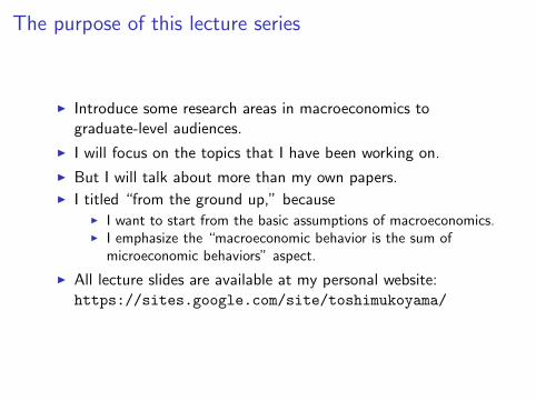
The purpose of this lecture series

I Introduce some research areas in macroeconomics tograduate-level audiences.

I I will focus on the topics that I have been working on.

I But I will talk about more than my own papers.I I titled “from the ground up,” because

I I want to start from the basic assumptions of macroeconomics.I I emphasize the “macroeconomic behavior is the sum of

microeconomic behaviors” aspect.

I All lecture slides are available at my personal website:https://sites.google.com/site/toshimukoyama/

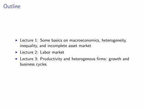
Outline

I Lecture 1: Some basics on macroeconomics, heterogeneity,inequality, and incomplete asset market

I Lecture 2: Labor market

I Lecture 3: Productivity and heterogenous firms: growth andbusiness cycles

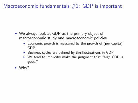
Macroeconomic fundamentals #1: GDP is important

I We always look at GDP as the primary object ofmacroeconomic study and macroeconomic policies.

I Economic growth is measured by the growth of (per-capita)GDP.

I Business cycles are defined by the fluctuations in GDP.I We tend to implicitly make the judgment that “high GDP is

good.”

I Why?

Macroeconomic fundamentals #1: GDP is important9�����2��*�����������������-����$'.���������� �$������������.����

Source: Stevenson and Wolfers (2008), from WP version.

I GDP is related to something we care about, for example,happiness.

I But why?

Macroeconomic fundamentals #1: GDP is important

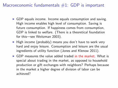
I GDP equals income. Income equals consumption and saving.High income enables high level of consumption. Saving isfuture consumption. If happiness comes from consumption,GDP is linked to welfare. (There is a theoretical foundationfor this—see Weitzman 2003).

I High income (probably) means you don’t have to work veryhard and enjoy leisure. Consumption and leisure are the usualingredients of utility function (Jones and Klenow 2011).

I GDP measures the value added traded in the market. What isspecial about trading in the market, as opposed to householdproduction or gift exchanges with neighbors? Perhaps becausein the market a higher degree of division of labor can beachieved?

Macroeconomic fundamentals #1: GDP is important

I Other possible reasons why GDP is correlated with happiness.I Low unemployment during the period of high GDP may itself

be valuable—the joy of “self-realization” by having a job.I Wealthier is healthier and live longer (Pritchett and Summers

1996).I Higher education may itself be valuable.I Democracy, freedom, etc. may themselves be valuable.I These things are a bit difficult to quantify (but still worthwhile

thinking).

I The basis for our implicit judgment lies in how GDP istranslated into happiness at the individual level.

Macroeconomic fundamentals #2: Aggregation

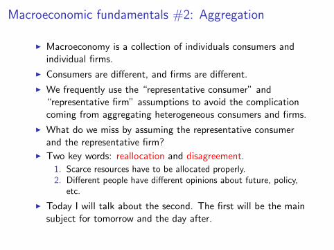
I Macroeconomy is a collection of individuals consumers andindividual firms.

I Consumers are different, and firms are different.

I We frequently use the “representative consumer” and“representative firm” assumptions to avoid the complicationcoming from aggregating heterogeneous consumers and firms.

I What do we miss by assuming the representative consumerand the representative firm?

I Two key words: reallocation and disagreement.

1. Scarce resources have to be allocated properly.2. Different people have different opinions about future, policy,

etc.

I Today I will talk about the second. The first will be the mainsubject for tomorrow and the day after.

Heterogeneity and aggregation

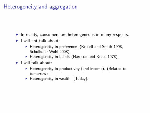
I In reality, consumers are heterogeneous in many respects.I I will not talk about:

I Heterogeneity in preferences (Krusell and Smith 1998,Schulhofer-Wohl 2008).

I Heterogeneity in beliefs (Harrison and Kreps 1978).

I I will talk about:I Heterogeneity in productivity (and income). (Related to

tomorrow)I Heterogeneity in wealth. (Today).

Wealth inequality

I There are three types of inequalities that people talk about:I Wealth inequality,I Income inequality,I Earnings inequality.I (There is also wage inequality, which is a big topic too, but I

will skip.)

I These inequalities are somewhat different:I In 2007, the Gini coefficient of was 0.82 for wealth, 0.58 for

income, and 0.64 for earnings (Dıaz-Gimenez et al. 2011).I They are not perfectly correlated. For example, old people

tend to have a lot of wealth but not much earnings.

I We have to be careful about which one matters, depending onthe context. In many macro models, what matters the most isthe wealth (lifetime wealth).

Does wealth inequality matter?I The answer is “no” in many macro models—a model with

large inequality behaves exactly the same as a model withsmall inequality (and has the same policy recommendations).

I This is because of the Gorman Aggregation Theorem.I If the indirect utility function is in the Gorman form

vi (p,Wi ) = ai (p) + b(p)Wi ,

where p is the price vector and Wi is the wealth. From Roy’sidentity, the Walrasian demand function is

ci (p,Wi ) = gi (p) + h(p)Wi ,

and thus the aggregate demand

C (p,Wi ) =∑i

gi (p) + h(p)∑i

Wi ,

so this depend only on the prices and the sum of wealth, sothe wealth distribution doesn’t matter for macroeconomicoutcome.

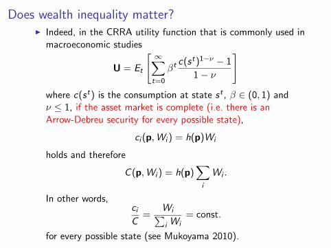
Does wealth inequality matter?I Indeed, in the CRRA utility function that is commonly used in

macroeconomic studies

U = Et

[ ∞∑t=0

βtc(st)1−ν − 1

1− ν

]where c(st) is the consumption at state st , β ∈ (0, 1) andν ≤ 1, if the asset market is complete (i.e. there is anArrow-Debreu security for every possible state),

ci (p,Wi ) = h(p)Wi

holds and therefore

C (p,Wi ) = h(p)∑i

Wi .

In other words,ciC

=Wi∑i Wi

= const.

for every possible state (see Mukoyama 2010).

Does wealth inequality matter?

I Thus in a model with complete asset market, everyonebehaves “proportionally” to each other. Unless there arewealth transfers, people feel the same about the change inenvironment or macroeconomic policy.

I This is one of the justifications of the use of representativeagent (and the use of GDP as the welfare criterion).

I A corollary is that the stochastic discount factor

βt(ci (s

t)

ci (s0)

)−νis common across i , thus everyone agrees on the assetvaluation, and all shareholders agree on the objective of thefirms that they own.

Does wealth inequality matter?

I So, in this world, the wealth inequality doesn’t matter, andeveryone behaves essentially the same way, no matter whathappens.

I This is a useful benchmark and convenient to analyze, but nottoo interesting/realistic.

I For example,I Everyone agrees on policy (except for the transfers)—no role

for politics.I Everyone is fully insured—losing a job, for example, is not a

big pain.

I In reality, not all states are covered by Arrow-Debreusecurities.

I People may not keep the promise (enforcement friction).I People may lie about what they do/did (information friction).

Does wealth inequality matter?When asset markets are incomplete, inequality matters.

I There has been a lot of analysis in the context of economicgrowth.

I The majority of the studies considers how the inequalitytranslates into growth through human capital accumulation.Sometimes entrepreneurship and “trickle-down” mechanism isemphasized.

I A less emphasized channel, which I think is perhaps moreimportant, is through politics. If wealth inequality is related tothe inequality of political power, the politics ↔ economicsfeedback may generate a serious stagnation. Mukoyama andPopov (2012) is not about the wealth heterogeneity, but anexample of how to model this feedback.

I In the business cycle context, my impression is thatI Many studies (starting Krusell and Smith 1998) show that the

aggregate business cycle dynamics is not much affected by themarket incompleteness.

I But it matters for normative evaluation of policies (see, forexample, Krusell, Mukoyama, Sahin, and Smith 2009).

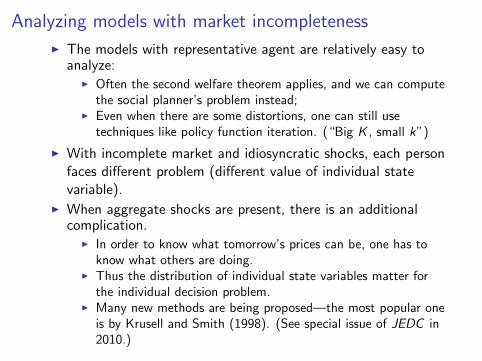
Analyzing models with market incompleteness

I The models with representative agent are relatively easy toanalyze:

I Often the second welfare theorem applies, and we can computethe social planner’s problem instead;

I Even when there are some distortions, one can still usetechniques like policy function iteration. (“Big K , small k”)

I With incomplete market and idiosyncratic shocks, each personfaces different problem (different value of individual statevariable).

I When aggregate shocks are present, there is an additionalcomplication.

I In order to know what tomorrow’s prices can be, one has toknow what others are doing.

I Thus the distribution of individual state variables matter forthe individual decision problem.

I Many new methods are being proposed—the most popular oneis by Krusell and Smith (1998). (See special issue of JEDC in2010.)

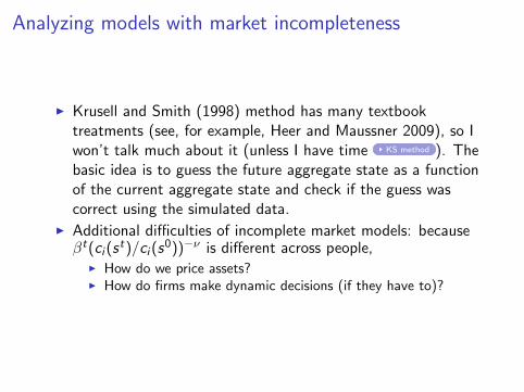
Analyzing models with market incompleteness

I Krusell and Smith (1998) method has many textbooktreatments (see, for example, Heer and Maussner 2009), so Iwon’t talk much about it (unless I have time KS method ). Thebasic idea is to guess the future aggregate state as a functionof the current aggregate state and check if the guess wascorrect using the simulated data.

I Additional difficulties of incomplete market models: becauseβt(ci (s

t)/ci (s0))−ν is different across people,

I How do we price assets?I How do firms make dynamic decisions (if they have to)?

A useful settingI Suppose that there are “aggregate Arrow securities” that gives

one unit of consumption good if the aggregate state is Z .I The consumer’s problem is to maximize

E

[ ∞∑t=0

βtct

1−ν

1− ν

]subject to

c +∑Z ′

QZ ′a′Z ′ = aZ + εz,Z

anda′Z ′ ≥ a for all Z ′.

I This is still an incomplete market model, since z is notspanned by the aggregate Arrow securities.

I With QZ ′ , any asset whose return depends only on aggregatestate can be priced (Krusell, Mukoyama, and Smith 2011).

I QZ ′ can be used to discount firm’s future profit (Krusell,Mukoyama, and Sahin 2010).

Main takeaways

I With complete asset market, standard macroeconomic modelswith wealth heterogeneity can be aggregated into arepresentative agent model.

I When the asset market is incomplete, inequality matters, andpeople may have different opinions about policy.

I Recent development in computational method has made thecomputation of this class of model easier.

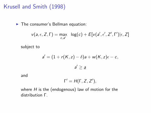
Krusell and Smith (1998)

I The consumer’s Bellman equation:

v(a, ε,Z , Γ) = maxc,a′

log(c) + E [v(a′, ε′,Z ′, Γ′)|ε,Z ]

subject to

a′ = (1 + r(K , z)− δ)a + w(K , z)ε− c,

a′ ≥ a

andΓ′ = H(Γ,Z ,Z ′),

where H is the (endogenous) law of motion for thedistribution Γ.

Krusell and Smith (1998)

1. Assume that the consumres only use a part of Γ as the information formaking a decision.

2. In particular, use K and assume that

log(K ′) =

{a0 + b0 log(K) if Z = g ,a1 + b1 log(K) if Z = b.

Guess a0, a1, b0, and b1.

3. Solvev(a, ε,Z ,K) = max

c,a′log(c) + E [v(a′, ε′,Z ′,K ′)|ε,Z ]

subject toa′ = (1 + r(K , z)− δ)a + w(K , z)ε− c,

a′ ≥ a,

and the above.

4. Simulate the economy.

5. Compare the simulated outcome of K with the law of motion. If the timeseries matches the guess, we found the REE. If not, modify the guess andrepeat.

back

References

I Dıaz-Gimenez, Javier, Andy Glover, and Jose-Vıactor Rıos-Rull (2011). “Factson the Distributions of Earnings, Income, and Wealth in the United States:2007 Update,” Federal Reserve Bank of Minneapolis Quarterly Review 34, 2-31.

I Harrison, J. Michael and David M. Kreps (1978). “Speculative InvestorBehavior in a Stock Market with Heterogeneous Expectations,” QuarterlyJournal of Economics 323-336.

I Heer, Burkhard and Alfred Maussner (2009). Dynamic General EquilibriumModeling, Springer.

I Jones, Charles I., and Peter J. Klenow (2011), Beyond GDP? Welfare acrossCountries and Time, mimeo.

I Krusell, Per, Toshihiko Mukoyama, and Aysegul Sahin (2010). “Labour-MarketMatching with Precautionary Savings and Aggregate Fluctuations, Review ofEconomic Studies 77 1477-1507.

I Krusell, Per, Toshihiko Mukoyama, Aysegul Sahin, and Anthony A. Smith Jr.(2009). “Revisiting the Welfare Effects of Eliminating Business Cycles,” Reviewof Economic Dynamics 12, 393-404.

I Krusell, Per, Toshihiko Mukoyama, and Anthony A. Smith Jr. (2011). “AssetPrices in a Huggett Economy, Journal of Economic Theory 146, 812-844.

References

I Krusell, Per and Anthony A. Smith Jr. (1998). “Income and WealthHeterogeneity in the Macroeconomy,” Journal of Political Economy 106,867-896.

I Mukoyama, Toshihiko (2010). “Welfare Effects of Unanticipated Policy Changeswith Complete Asset Markets,” Economics Letters 109, 134-138.

I Mukoyama, Toshihiko and Latchezar Popov (2012). “The Political Economy ofEntry Barriers,” mimeo.

I Pritchett, Lant and Lawrence H. Summers (1996), “Wealthier is Healthier,”Journal of Human Resources 31, 841-868.

I Schulhofer-Wohl, Sam (2008). “Heterogeneous Risk Preferences and theWelfare Cost of Business Cycles, Review of Economic Dynamics 11, 761-780.

I Stevenson, Betsey and Justin Wolfers (2008). “Economic Growth andSubjective Well-Being: Reassessing the Easterlin Paradox,” Brookings Papers onEconomic Activity 2008 Spring.

I Weitzman, Martin L. (2003). Income, Wealth, and Maximum Principle,Cambridge, Harvard University Press.