macmahon’s partition analysis v: bijections, recursions ... · macmahon’s partition analysis v:...
TRANSCRIPT
MacMahon’s Partition Analysis V:Bijections, Recursions, and Magic Squares
George E. Andrews1?, Peter Paule2, Axel Riese3??, and Volker Strehl4? ? ?
1 Department of MathematicsThe Pennsylvania State UniversityUniversity Park, PA 16802, [email protected]
2 Research Institute for Symbolic ComputationJohannes Kepler University LinzA–4040 Linz, [email protected]
3 Research Institute for Symbolic ComputationJohannes Kepler University LinzA–4040 Linz, [email protected]
4 Computer Science Institute-Informatik 8Friedrich-Alexander-Universitat Erlangen-NurnbergD–91058 Erlangen, [email protected]
Dedicated to Professor A. Kerber at the occasion of his 60th birthday
Abstract. A significant portion of MacMahon’s famous book “Combinatory Anal-ysis” is devoted to the development of “Partition Analysis” as a computationalmethod for solving problems in connection with linear homogeneous diophantineinequalities and equations, respectively. Nevertheless, MacMahon’s ideas have notreceived due attention with the exception of work by Richard Stanley. A long rangeobject of a series of articles is to change this situation by demonstrating the powerof MacMahon’s method in current combinatorial and partition-theoretic research.The renaissance of MacMahon’s technique partly is due to the fact that it is ideallysuited for being supplemented by modern computer algebra methods. In this paperwe illustrate the use of Partition Analysis and of the corresponding package Omega
by focusing on three different aspects of combinatorial work: the construction ofbijections (for the Refined Lecture Hall Partition Theorem), exploitation of recur-sive patterns (for Cayley compositions), and finding nonnegative integer solutionsof linear systems of diophantine equations (for magic squares of size 3).
? Partially supported by National Science Foundation Grant DMS-9870060.?? Supported by SFB-grant F1305 of the Austrian FWF.
? ? ? Supported by a visiting researcher grant of the J. Kepler University Linz.

2 George E. Andrews, Peter Paule, Axel Riese, and Volker Strehl
1 Introduction
The initial motive for the revival of MacMahon’s Partition Analysis was thebeautiful refinement of a classic result due to Euler – the number of partitionsof N into distinct parts equals the number of partitions of N into odd parts[1, p. 5] – that was discovered by M. Bousquet-Melou and K. Eriksson [7]only recently:
Theorem 1 (“Lecture Hall Partition Theorem”). The number of par-titions of N of the form N = b1 + b2 + · · ·+ bn wherein
bnn≥ bn−1
n− 1≥ · · · ≥ b1
1≥ 0
equals the number of partitions of N into odd parts each ≤ 2n− 1.
Note that in lecture hall partitions some parts can be 0. For example, ifN = 13 and n = 3 we have the 10 lecture hall partitions 0+0+13, 0+1+12,0 + 2 + 11, 0 + 3 + 10, 1 + 2 + 10, 0 + 4 + 9, 1 + 3 + 9, 0 + 5 + 8, 1 + 4 + 8,and 2 + 4 + 7. On the other hand there are also 10 partitions of N = 13 intoparts from 1, 3, 5, namely 103152, 133052, 123251, 153151, 183051, 113450,143350, 173250, 1103150, and 1133050.
The same authors also derived a further refinement of Euler’s classic re-sult; see the “Refined Lecture Hall Partition Theorem” (Theorem 17) below.Section 2 will be devoted to the construction of a bijective proof of it.
In [7] Bousquet-Melou and Eriksson gave two different proofs of this the-orem, one using Bott’s formula for the affine Coxeter group Cn, and oneof bijective-combinatorial nature. In [3] the first named author presented aproof following an entirely different approach. Namely, an approach which isbased on the observation that MacMahon’s Partition Analysis, surveyed in[12, Vol. 2, Sect. VIII, pp. 91–170], is perfectly tailored for theorems of thiskind. In order to illustrate this point, recall the definition of MacMahon’sOmega operator Ω=.
Definition 2. The operator Ω= is given by
Ω=
∞∑s1=−∞
· · ·∞∑
sr=−∞As1,...,srλ
s11 · · ·λsrr :=
∞∑s1=0
· · ·∞∑sr=0
As1,...,sr ,
where the domain of the As1,...,sr is the field of rational functions over Cin several complex variables and the λi are restricted to annuli of the form1− ε < |λi| < 1 + ε.
Remark 3. It is convenient to treat everything involved analytically ratherthan formally because the method relies on unique Laurent series represen-tations of a variety of rational functions. For a more detailed discussion ofthis aspect, the interested reader is referred to [4].
MacMahon’s Partition Analysis V 3
Let us now consider the instance n = 3 of Theorem 1. Obviously, thecoefficient of qN in
1(1− q)(1− q3)(1− q5)
(1)
equals the number of partitions of N into odd parts each ≤ 5. On the otherhand, the coefficient of qN in
Ω=
∑b1,b2,b3≥0
λ2b3−3b21 λb2−2b1
2 qb1+b2+b3 (2)
gives exactly the number of the desired lecture hall partitions for n beingfixed to 3. Note that due to the Omega operator Ω= only those partitionsb1 + b2 + b3 = N are counted for which 2b3 − 3b2 ≥ 0 and b2 − 2b1 ≥ 0. Bygeometric series expansion the triple sum can be brought into product form,which means that expression (2) can be rewritten as
Ω=
1
(1− λ21 q)(1− λ2 q
λ31
)(1− q
λ22
) . (3)
where the factors in the denominator correspond to b3, b2, b1 in this order.Therefore all what remains for proving the Lecture Hall Partition Theo-
rem for n = 3 is to show equality of the generating function expressions (1)and (3). For doing so, MacMahon introduced a catalogue of rules that de-scribe the elimination of the λ-parameters involved. As an example, we stateone of these rules in form of a lemma.
Lemma 4. For any integer s ≥ 0,
Ω=
1(1− λx)
(1− y
λs
) =1
(1− x)(1− xsy).
Proof. By geometric series expansion the left hand side equals
Ω=
∑i,j≥0
λi−sjxiyj = Ω=
∑j,k≥0
λkxsj+kyj ,
where the summation parameter i has been replaced by sj + k. But now Ω=sets λ to 1, which completes the proof. ut
With this lemma in hand, the proof of “(1) = (3)” reduces to successiveelimination of the Ω=-parameters λ1 and λ2.
Proof (of the Lecture Hall Partition Theorem for j = 3). Split (3) additivelyinto two parts by applying partial fraction decomposition 1/((1 − λ1z)(1 +λ1z)) = 1/(2(1 − λ1z)) + 1/(2(1 + λ1z)) to the term 1/(1 − λ2
1q). Then byusing Lemma 4 eliminate from both summands the Ω=-parameter λ1. Forthe last step one observes that Lemma 4 can be applied again in order toeliminate λ2; this way one arrives at (1). ut
4 George E. Andrews, Peter Paule, Axel Riese, and Volker Strehl
Already this particular example suggests that MacMahon’s approach is anideal candidate for being supplemented by modern computer algebra meth-ods. But rather than implementing tables of rules – as, for example, the listof twelve fundamental evaluations given by MacMahon [12, Vol. II, pp. 102–103] – in [4, Theorem 2] we explain how this can be achieved “in one stroke”by a fairly general setting based on the “fundamental recurrence” for the Ω=operator. Using the procedures from the Mathematica package Omega, theproblem of showing “(1) = (3)” is solved as follows:
We put the file Omega.m (together with the file Readme.txt) in the samedirectory in which we run our Mathematica session. After invoking Mathe-matica we load the package:
In[1]:= <<Omega.mAxel Riese’s Omega implementation version 1.3 loaded
Now the proof of Theorem 1 for n = 3 can simply be done as follows.First we input the expression the Ω= operator acts on; see (3). Then we callthe OR-procedure to eliminate the λ-variables λ1 and λ2:
In[2]:= f = 1 / ((1-λ1^2 q)(1-λ2 q/λ1^3)(1-q/λ2^2))
Out[2]=1(
1− λ2 qλ13
)(1− λ12 q)
(1− q
λ22
)In[3]:= OR[f, λ1]
Out[3]=1 + λ2 q3
(1− q)(1− q
λ22
)(1− λ22 q5)
In[4]:= OR[%, λ2]
Out[4]=1
(1− q) (1− q3) (1− q5)
This proves the equality in question.More information (theoretical background, usage, etc.) about the Omega
package can be found in [4]. In this paper we focus on concrete applicationsconcerning the construction of bijections, exploitation of recursive patterns,and finding nonnegative integer solutions of linear systems of diophantineequations.
In Sect. 2 we illustrate how the Omega package and, more generally, Par-tition Analysis can be used for the construction of a bijective proof, Propo-sition 14 and Theorem 19, for the Refined Lecture Hall Partition Theorem(Theorem 17), a refinement of Theorem 1 above. To this end we need an-other essential ingredient, namely an involution, defined in Sect. 2.5, that is
MacMahon’s Partition Analysis V 5
equivalent to an involution discovered by Bousquet-Melou and Eriksson in [8,Prop. 3.4].
In Sect. 3 we deal with a classical type of compositions that have beenintroduced and studied by A. Cayley [9]. Here the application of the Omegapackage leads to the discovery of a recursive pattern that enables to finda surprising generating function representation, Theorem 29, which encodesthe solution to Cayley’s problem.
Finally, in Sect. 4 we briefly describe how MacMahon’s technique works forfinding nonnegative integer solutions of systems of linear homogeneous dio-phantine equations. Instead of following MacMahon’s table look-up approach,we again achieve elimination “in one stroke” by deriving a suitable analogue(Theorem 33) of the “fundamental recurrence” developed in [4, Theorem 2]for diophantine inequalities. We illustrate our Mathematica implementationby revisiting a section of MacMahon’s book [12, Vol. 2, Sect. 407, p. 161].
2 A Lecture Hall Bijection
Following [3], for n ≥ 2 let us define
fn(y1, . . . , yn) =∑
bnn ≥
bn−1n−1 ≥···≥
b11 ≥0
yb11 yb22 · · · ybnn . (4)
We note that in [3] the notation Fn−1,0(yn, yn−1, . . . , y1) is used instead offn(y1, . . . , yn).
The generating function version of Theorem 1 then is
fn(q, . . . , q) =n∏k=1
11− q2k−1
(5)
which was proved in [3] by using Partition Analysis. In order to give a flavorof the mechanism of MacMahon’s method, we briefly sketch how this hasbeen achieved.
By introducing parameters λ1 up to λn−1 where the jth lecture hall condi-tion (j−1) bj ≥ j bj−1 is represented by a factor λ(j−1) bj−j bj−1
n−j+1 , (2 ≤ j ≤ n),the generating function expression (4), is encoded as an Ω=-expression:
fn(y1, . . . , yn) = Ω=
1
(1− λn−11 yn)
(1− λn−2
2λn1
yn−1
)· 1(
1− λn−33
λn−12
yn−2
)· · ·(1− λn−1
λ3n−2
y2
)(1− y1
λ2n−1
) .
6 George E. Andrews, Peter Paule, Axel Riese, and Volker Strehl
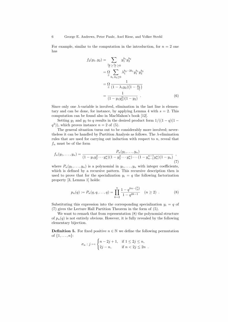
For example, similar to the computation in the introduction, for n = 2 onehas
f2(y1, y2) =∑
b22 ≥
b11 ≥0
yb11 yb22
= Ω=
∑b1,b2≥0
λb2−2b11 yb11 y
b22
= Ω=
1(1− λ1y2)
(1− y1
λ21
)=
1(1− y1y2
2)(1− y2). (6)
Since only one λ-variable is involved, elimination in the last line is elemen-tary and can be done, for instance, by applying Lemma 4 with s = 2. Thiscomputation can be found also in MacMahon’s book [12].
Setting y1 and y2 to q results in the desired product form 1/((1− q)(1−q3)), which proves instance n = 2 of (5).
The general situation turns out to be considerably more involved; never-theless it can be handled by Partition Analysis as follows. The λ-eliminationrules that are used for carrying out induction with respect to n, reveal thatfn must be of the form
fn(y1, . . . , yn) =Pn(y1, . . . , yn)
(1− y1y22 · · · ynn)(1− y2
2 · · · ynn) · · · (1− yn−1n−1y
nn)(1− yn)
,
(7)where Pn(y1, . . . , yn) is a polynomial in y1, . . . , yn with integer coefficients,which is defined by a recursive pattern. This recursive description then isused to prove that for the specialization yi = q the following factorizationproperty [3, Lemma 1] holds:
pn(q) := Pn(q, q, . . . , q) =n∏k=2
1− qkn−(k2)
1− q2k−1(n ≥ 2) . (8)
Substituting this expression into the corresponding specialization yi = q of(7) gives the Lecture Hall Partition Theorem in the form of (5).
We want to remark that from representation (8) the polynomial structureof pn(q) is not entirely obvious. However, it is fully revealed by the followingelementary bijection.
Definition 5. For fixed positive n ∈ N we define the following permutationof 1, . . . , n:
σn : j 7→
n− 2j + 1, if 1 ≤ 2j ≤ n,2j − n, if n < 2j ≤ 2n .
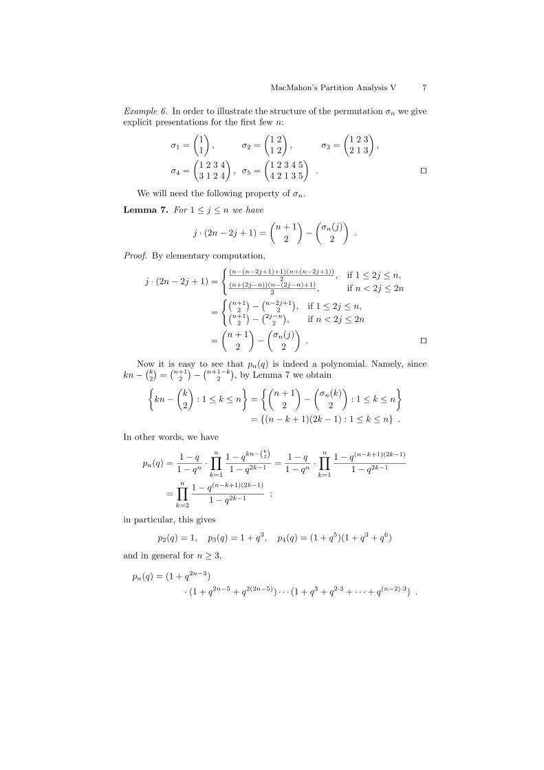
MacMahon’s Partition Analysis V 7
Example 6. In order to illustrate the structure of the permutation σn we giveexplicit presentations for the first few n:
σ1 =(
11
), σ2 =
(1 21 2
), σ3 =
(1 2 32 1 3
),
σ4 =(
1 2 3 43 1 2 4
), σ5 =
(1 2 3 4 54 2 1 3 5
). ut
We will need the following property of σn.
Lemma 7. For 1 ≤ j ≤ n we have
j · (2n− 2j + 1) =(n+ 1
2
)−(σn(j)
2
).
Proof. By elementary computation,
j · (2n− 2j + 1) =
(n−(n−2j+1)+1)(n+(n−2j+1))
2 , if 1 ≤ 2j ≤ n,(n+(2j−n))(n−(2j−n)+1)
2 , if n < 2j ≤ 2n
=
(n+1
2
)−(n−2j+1
2
), if 1 ≤ 2j ≤ n,(
n+12
)−(
2j−n2
), if n < 2j ≤ 2n
=(n+ 1
2
)−(σn(j)
2
). ut
Now it is easy to see that pn(q) is indeed a polynomial. Namely, sincekn−
(k2
)=(n+1
2
)−(n+1−k
2
), by Lemma 7 we obtain
kn−(k
2
): 1 ≤ k ≤ n
=(
n+ 12
)−(σn(k)
2
): 1 ≤ k ≤ n
= (n− k + 1)(2k − 1) : 1 ≤ k ≤ n .
In other words, we have
pn(q) =1− q1− qn
·n∏k=1
1− qkn−(k2)
1− q2k−1=
1− q1− qn
·n∏k=1
1− q(n−k+1)(2k−1)
1− q2k−1
=n∏k=2
1− q(n−k+1)(2k−1)
1− q2k−1;
in particular, this gives
p2(q) = 1, p3(q) = 1 + q3, p4(q) = (1 + q5)(1 + q3 + q6)
and in general for n ≥ 3,
pn(q) = (1 + q2n−3)
· (1 + q2n−5 + q2(2n−5)) · · · (1 + q3 + q2·3 + · · ·+ q(n−2)·3) .
8 George E. Andrews, Peter Paule, Axel Riese, and Volker Strehl
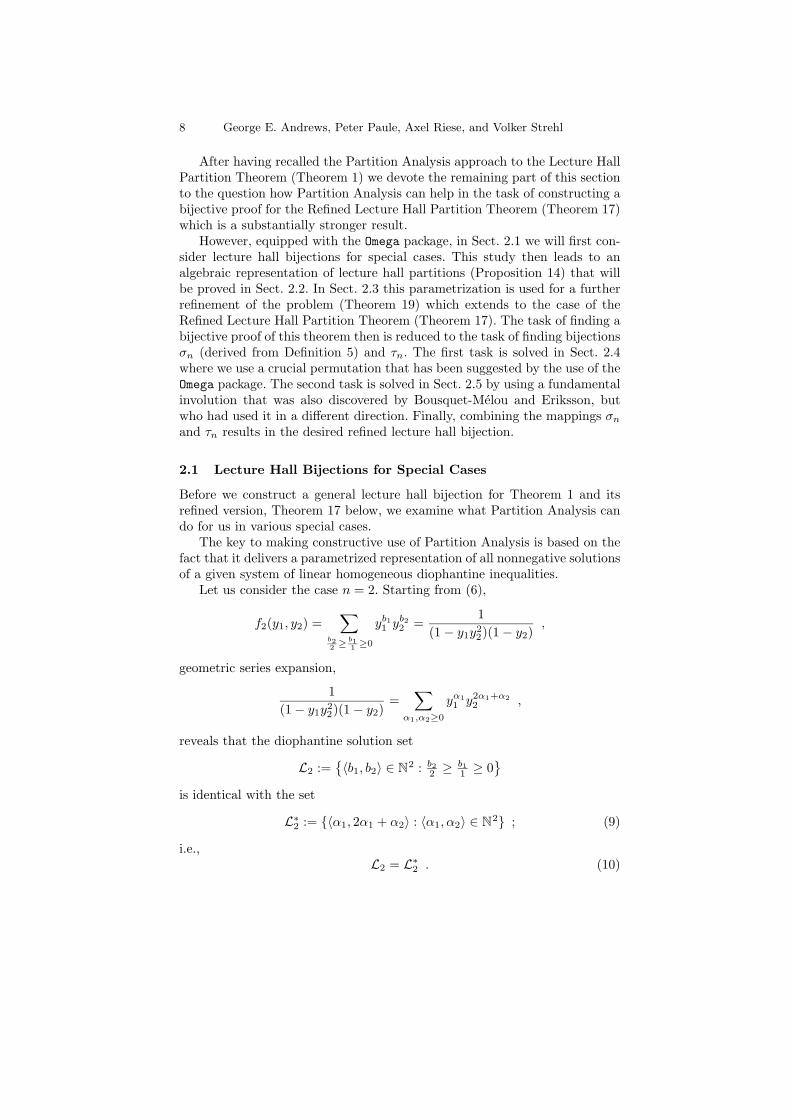
After having recalled the Partition Analysis approach to the Lecture HallPartition Theorem (Theorem 1) we devote the remaining part of this sectionto the question how Partition Analysis can help in the task of constructing abijective proof for the Refined Lecture Hall Partition Theorem (Theorem 17)which is a substantially stronger result.
However, equipped with the Omega package, in Sect. 2.1 we will first con-sider lecture hall bijections for special cases. This study then leads to analgebraic representation of lecture hall partitions (Proposition 14) that willbe proved in Sect. 2.2. In Sect. 2.3 this parametrization is used for a furtherrefinement of the problem (Theorem 19) which extends to the case of theRefined Lecture Hall Partition Theorem (Theorem 17). The task of finding abijective proof of this theorem then is reduced to the task of finding bijectionsσn (derived from Definition 5) and τn. The first task is solved in Sect. 2.4where we use a crucial permutation that has been suggested by the use of theOmega package. The second task is solved in Sect. 2.5 by using a fundamentalinvolution that was also discovered by Bousquet-Melou and Eriksson, butwho had used it in a different direction. Finally, combining the mappings σnand τn results in the desired refined lecture hall bijection.
2.1 Lecture Hall Bijections for Special Cases
Before we construct a general lecture hall bijection for Theorem 1 and itsrefined version, Theorem 17 below, we examine what Partition Analysis cando for us in various special cases.
The key to making constructive use of Partition Analysis is based on thefact that it delivers a parametrized representation of all nonnegative solutionsof a given system of linear homogeneous diophantine inequalities.
Let us consider the case n = 2. Starting from (6),
f2(y1, y2) =∑
b22 ≥
b11 ≥0
yb11 yb22 =
1(1− y1y2
2)(1− y2),
geometric series expansion,
1(1− y1y2
2)(1− y2)=
∑α1,α2≥0
yα11 y2α1+α2
2 ,
reveals that the diophantine solution set
L2 :=〈b1, b2〉 ∈ N2 : b22 ≥
b11 ≥ 0
is identical with the set
L∗2 := 〈α1, 2α1 + α2〉 : 〈α1, α2〉 ∈ N2 ; (9)
i.e.,L2 = L∗2 . (10)
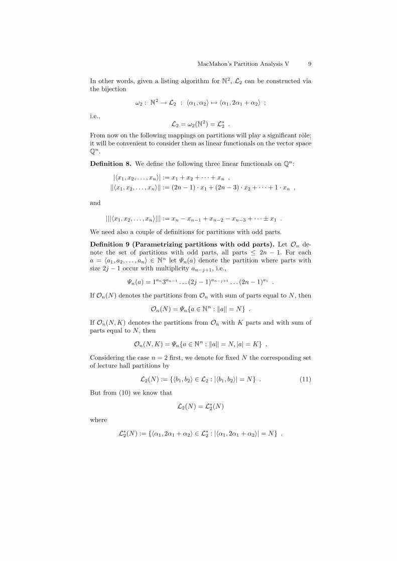
MacMahon’s Partition Analysis V 9
In other words, given a listing algorithm for N2, L2 can be constructed viathe bijection
ω2 : N2 → L2 : 〈α1, α2〉 7→ 〈α1, 2α1 + α2〉 ;
i.e.,L2 = ω2(N2) = L∗2 .
From now on the following mappings on partitions will play a significant role;it will be convenient to consider them as linear functionals on the vector spaceQn.
Definition 8. We define the following three linear functionals on Qn:
|〈x1, x2, . . . , xn〉| := x1 + x2 + · · ·+ xn ,
‖〈x1, x2, . . . , xn〉‖ := (2n− 1) · x1 + (2n− 3) · x2 + · · ·+ 1 · xn ,
and
|||〈x1, x2, . . . , xn〉||| := xn − xn−1 + xn−2 − xn−3 + · · · ± x1 .
We need also a couple of definitions for partitions with odd parts.
Definition 9 (Parametrizing partitions with odd parts). Let On de-note the set of partitions with odd parts, all parts ≤ 2n − 1. For eacha = 〈a1, a2, . . . , an〉 ∈ Nn let Ψn(a) denote the partition where parts withsize 2j − 1 occur with multiplicity an−j+1, i.e.,
Ψn(a) = 1an3an−1 . . . (2j − 1)an−j+1 . . . (2n− 1)a1 .
If On(N) denotes the partitions from On with sum of parts equal to N , then
On(N) = Ψna ∈ Nn : ‖a‖ = N .
If On(N,K) denotes the partitions from On with K parts and with sum ofparts equal to N , then
On(N,K) = Ψna ∈ Nn : ‖a‖ = N, |a| = K .
Considering the case n = 2 first, we denote for fixed N the corresponding setof lecture hall partitions by
L2(N) := 〈b1, b2〉 ∈ L2 : |〈b1, b2〉| = N . (11)
But from (10) we know that
L2(N) = L∗2(N)
where
L∗2(N) := 〈α1, 2α1 + α2〉 ∈ L∗2 : |〈α1, 2α1 + α2〉| = N .
10 George E. Andrews, Peter Paule, Axel Riese, and Volker Strehl
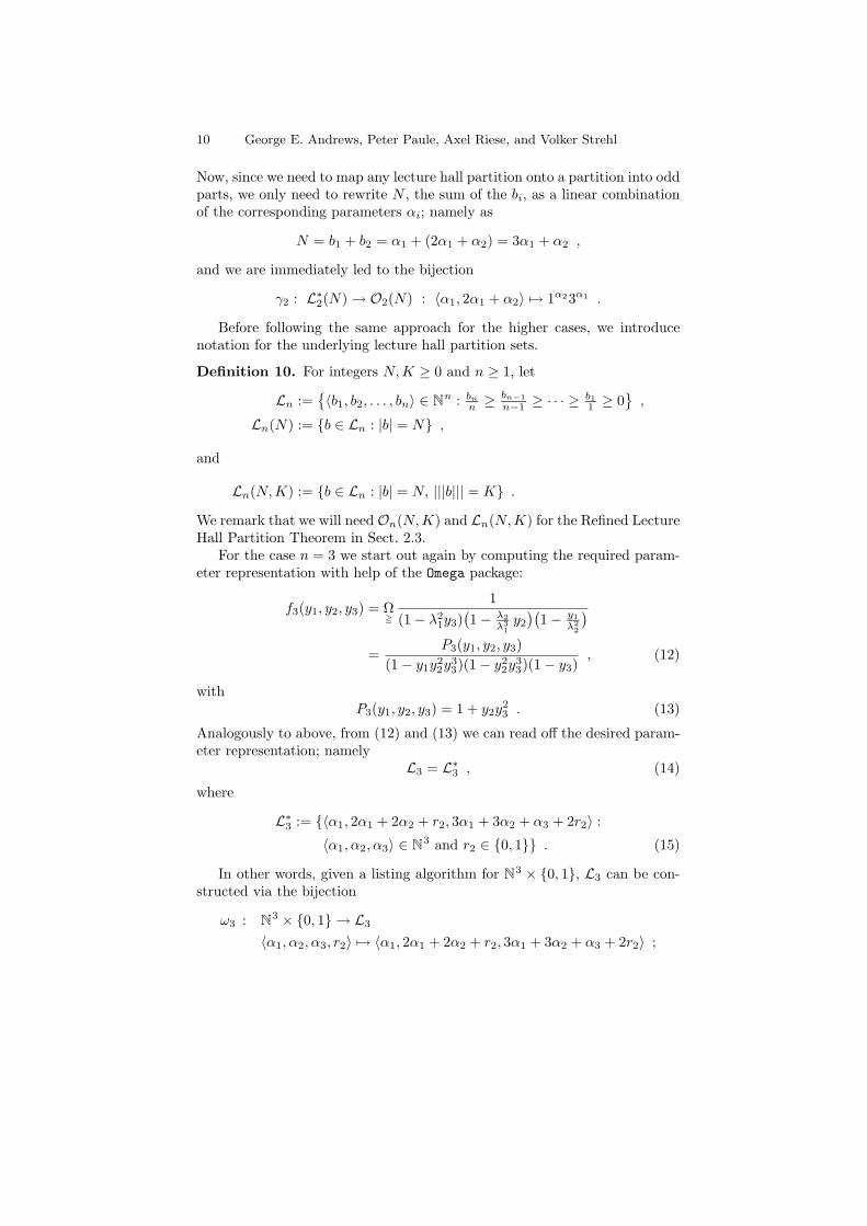
Now, since we need to map any lecture hall partition onto a partition into oddparts, we only need to rewrite N , the sum of the bi, as a linear combinationof the corresponding parameters αi; namely as
N = b1 + b2 = α1 + (2α1 + α2) = 3α1 + α2 ,
and we are immediately led to the bijection
γ2 : L∗2(N)→ O2(N) : 〈α1, 2α1 + α2〉 7→ 1α23α1 .
Before following the same approach for the higher cases, we introducenotation for the underlying lecture hall partition sets.
Definition 10. For integers N,K ≥ 0 and n ≥ 1, let
Ln :=〈b1, b2, . . . , bn〉 ∈ Nn : bnn ≥
bn−1n−1 ≥ · · · ≥
b11 ≥ 0
,
Ln(N) := b ∈ Ln : |b| = N ,
and
Ln(N,K) := b ∈ Ln : |b| = N, |||b||| = K .
We remark that we will need On(N,K) and Ln(N,K) for the Refined LectureHall Partition Theorem in Sect. 2.3.
For the case n = 3 we start out again by computing the required param-eter representation with help of the Omega package:
f3(y1, y2, y3) = Ω=
1(1− λ2
1y3)(1− λ2
λ31y2
)(1− y1
λ22
)=
P3(y1, y2, y3)(1− y1y2
2y33)(1− y2
2y33)(1− y3)
, (12)
withP3(y1, y2, y3) = 1 + y2y
23 . (13)
Analogously to above, from (12) and (13) we can read off the desired param-eter representation; namely
L3 = L∗3 , (14)
where
L∗3 := 〈α1, 2α1 + 2α2 + r2, 3α1 + 3α2 + α3 + 2r2〉 :
〈α1, α2, α3〉 ∈ N3 and r2 ∈ 0, 1 . (15)
In other words, given a listing algorithm for N3 × 0, 1, L3 can be con-structed via the bijection
ω3 : N3 × 0, 1 → L3
〈α1, α2, α3, r2〉 7→ 〈α1, 2α1 + 2α2 + r2, 3α1 + 3α2 + α3 + 2r2〉 ;
MacMahon’s Partition Analysis V 11
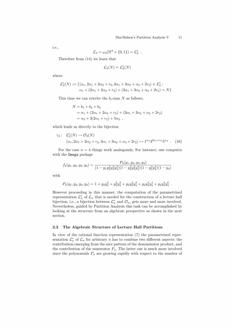
i.e.,L3 = ω3(N3 × 0, 1) = L∗3 .
Therefore from (14) we learn that
L3(N) = L∗3(N)
where
L∗3(N) := 〈α1, 2α1 + 2α2 + r2, 3α1 + 3α2 + α3 + 2r2〉 ∈ L∗3 :α1 + (2α1 + 2α2 + r2) + (3α1 + 3α2 + α3 + 2r2) = N .
This time we can rewrite the bi-sum N as follows,
N = b1 + b2 + b3
= α1 + (2α1 + 2α2 + r2) + (3α1 + 3α2 + α3 + 2r2)= α3 + 3(2α1 + r2) + 5α2 ,
which leads us directly to the bijection
γ3 : L∗3(N)→ O3(N)
〈α1, 2α1 + 2α2 + r2, 3α1 + 3α2 + α3 + 2r2〉 7→ 1α332α1+r25α2 . (16)
For the case n = 4 things work analogously. For instance, one computeswith the Omega package
f4(y1, y2, y3, y4) =P4(y1, y2, y3, y4)
(1− y1y22y
33y
44)(1− y2
2y33y
44)(1− y3
3y44)(1− y4)
with
P4(y1, y2, y3, y4) = 1 + y3y24 + y2
3y34 + y2y
23y
34 + y2y
33y
44 + y2y
43y
64 .
However proceeding in this manner, the computation of the parametrizedrepresentation L∗n of Ln that is needed for the construction of a lecture hallbijection, i.e., a bijection between L∗n and On, gets more and more involved.Nevertheless, guided by Partition Analysis this task can be accomplished bylooking at the structure from an algebraic perspective as shown in the nextsection.
2.2 The Algebraic Structure of Lecture Hall Partitions
In view of the rational function representation (7) the parametrized repre-sentation L∗n of Ln for arbitrary n has to combine two different aspects: thecontribution emerging from the nice pattern of the denominator product, andthe contribution of the numerator Pn. The latter one is much more involvedsince the polynomials Pn are growing rapidly with respect to the number of
12 George E. Andrews, Peter Paule, Axel Riese, and Volker Strehl
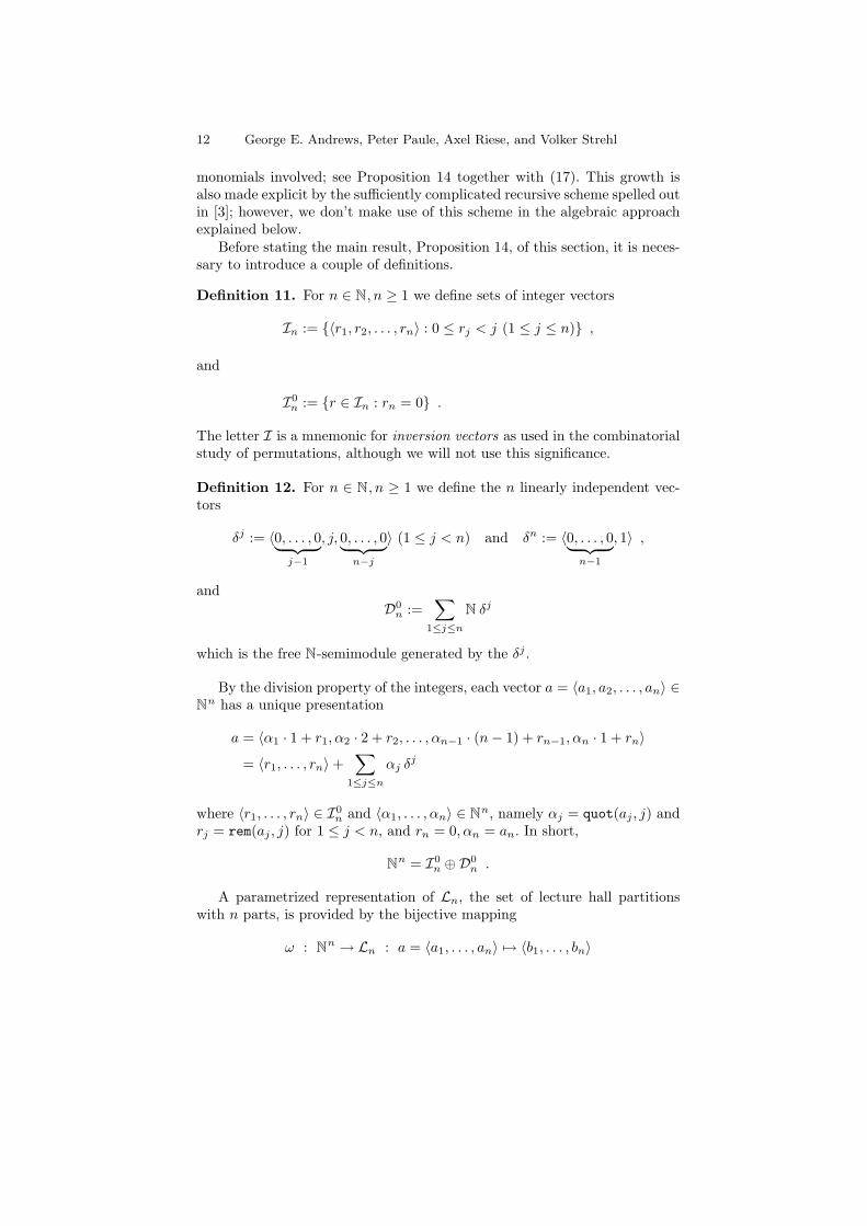
monomials involved; see Proposition 14 together with (17). This growth isalso made explicit by the sufficiently complicated recursive scheme spelled outin [3]; however, we don’t make use of this scheme in the algebraic approachexplained below.
Before stating the main result, Proposition 14, of this section, it is neces-sary to introduce a couple of definitions.
Definition 11. For n ∈ N, n ≥ 1 we define sets of integer vectors
In := 〈r1, r2, . . . , rn〉 : 0 ≤ rj < j (1 ≤ j ≤ n) ,
and
I0n := r ∈ In : rn = 0 .
The letter I is a mnemonic for inversion vectors as used in the combinatorialstudy of permutations, although we will not use this significance.
Definition 12. For n ∈ N, n ≥ 1 we define the n linearly independent vec-tors
δj := 〈0, . . . , 0︸ ︷︷ ︸j−1
, j, 0, . . . , 0︸ ︷︷ ︸n−j
〉 (1 ≤ j < n) and δn := 〈0, . . . , 0︸ ︷︷ ︸n−1
, 1〉 ,
andD0n :=
∑1≤j≤n
N δj
which is the free N-semimodule generated by the δj .
By the division property of the integers, each vector a = 〈a1, a2, . . . , an〉 ∈Nn has a unique presentation
a = 〈α1 · 1 + r1, α2 · 2 + r2, . . . , αn−1 · (n− 1) + rn−1, αn · 1 + rn〉
= 〈r1, . . . , rn〉+∑
1≤j≤n
αj δj
where 〈r1, . . . , rn〉 ∈ I0n and 〈α1, . . . , αn〉 ∈ Nn, namely αj = quot(aj , j) and
rj = rem(aj , j) for 1 ≤ j < n, and rn = 0, αn = an. In short,
Nn = I0
n ⊕D0n .
A parametrized representation of Ln, the set of lecture hall partitionswith n parts, is provided by the bijective mapping
ω : Nn → Ln : a = 〈a1, . . . , an〉 7→ 〈b1, . . . , bn〉
MacMahon’s Partition Analysis V 13
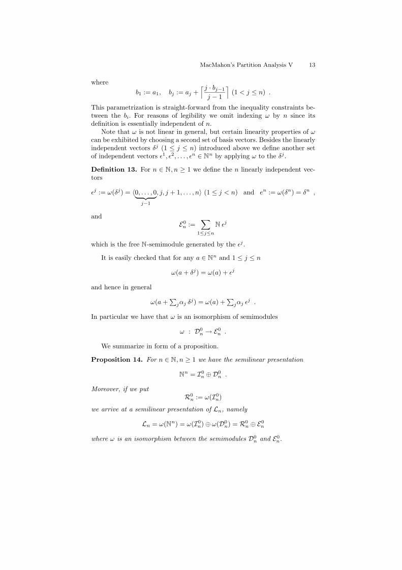
whereb1 := a1, bj := aj +
⌈j · bj−1
j − 1
⌉(1 < j ≤ n) .
This parametrization is straight-forward from the inequality constraints be-tween the bi. For reasons of legibility we omit indexing ω by n since itsdefinition is essentially independent of n.
Note that ω is not linear in general, but certain linearity properties of ωcan be exhibited by choosing a second set of basis vectors. Besides the linearlyindependent vectors δj (1 ≤ j ≤ n) introduced above we define another setof independent vectors ε1, ε2, . . . , εn ∈ Nn by applying ω to the δj .
Definition 13. For n ∈ N, n ≥ 1 we define the n linearly independent vec-tors
εj := ω(δj) = 〈0, . . . , 0︸ ︷︷ ︸j−1
, j, j + 1, . . . , n〉 (1 ≤ j < n) and en := ω(δn) = δn ,
andE0n :=
∑1≤j≤n
N εj
which is the free N-semimodule generated by the εj .
It is easily checked that for any a ∈ Nn and 1 ≤ j ≤ n
ω(a+ δj) = ω(a) + εj
and hence in general
ω(a+∑jαj δ
j) = ω(a) +∑jαj ε
j .
In particular we have that ω is an isomorphism of semimodules
ω : D0n → E0
n .
We summarize in form of a proposition.
Proposition 14. For n ∈ N, n ≥ 1 we have the semilinear presentation
Nn = I0
n ⊕D0n .
Moreover, if we putR0n := ω(I0
n)
we arrive at a semilinear presentation of Ln, namely
Ln = ω(Nn) = ω(I0n)⊕ ω(D0
n) = R0n ⊕ E0
n
where ω is an isomorphism between the semimodules D0n and E0
n.
14 George E. Andrews, Peter Paule, Axel Riese, and Volker Strehl
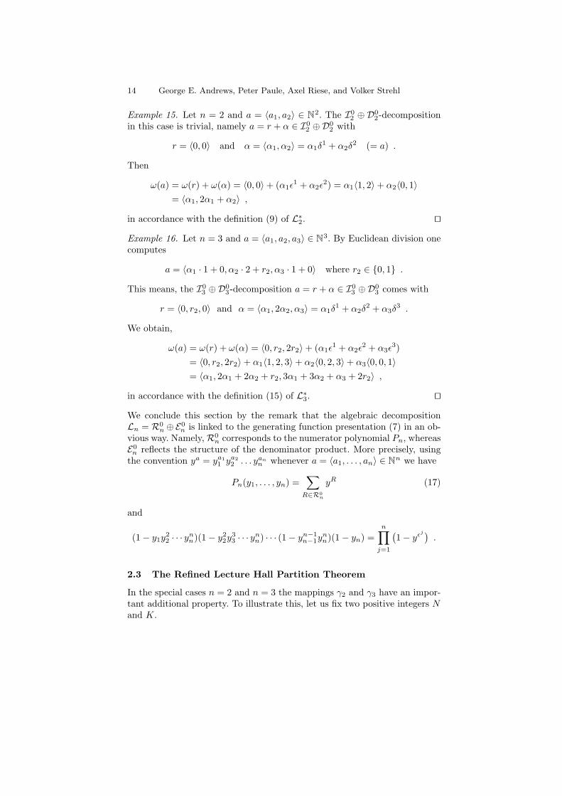
Example 15. Let n = 2 and a = 〈a1, a2〉 ∈ N2. The I02 ⊕ D0
2-decompositionin this case is trivial, namely a = r + α ∈ I0
2 ⊕D02 with
r = 〈0, 0〉 and α = 〈α1, α2〉 = α1δ1 + α2δ
2 (= a) .
Then
ω(a) = ω(r) + ω(α) = 〈0, 0〉+ (α1ε1 + α2ε
2) = α1〈1, 2〉+ α2〈0, 1〉= 〈α1, 2α1 + α2〉 ,
in accordance with the definition (9) of L∗2. ut
Example 16. Let n = 3 and a = 〈a1, a2, a3〉 ∈ N3. By Euclidean division onecomputes
a = 〈α1 · 1 + 0, α2 · 2 + r2, α3 · 1 + 0〉 where r2 ∈ 0, 1 .
This means, the I03 ⊕D0
3-decomposition a = r + α ∈ I03 ⊕D0
3 comes with
r = 〈0, r2, 0〉 and α = 〈α1, 2α2, α3〉 = α1δ1 + α2δ
2 + α3δ3 .
We obtain,
ω(a) = ω(r) + ω(α) = 〈0, r2, 2r2〉+ (α1ε1 + α2ε
2 + α3ε3)
= 〈0, r2, 2r2〉+ α1〈1, 2, 3〉+ α2〈0, 2, 3〉+ α3〈0, 0, 1〉= 〈α1, 2α1 + 2α2 + r2, 3α1 + 3α2 + α3 + 2r2〉 ,
in accordance with the definition (15) of L∗3. ut
We conclude this section by the remark that the algebraic decompositionLn = R0
n ⊕E0n is linked to the generating function presentation (7) in an ob-
vious way. Namely,R0n corresponds to the numerator polynomial Pn, whereas
E0n reflects the structure of the denominator product. More precisely, using
the convention ya = ya11 ya2
2 . . . yann whenever a = 〈a1, . . . , an〉 ∈ Nn we have
Pn(y1, . . . , yn) =∑R∈R0
n
yR (17)
and
(1− y1y22 · · · ynn)(1− y2
2y33 · · · ynn) · · · (1− yn−1
n−1ynn)(1− yn) =
n∏j=1
(1− yε
j).
2.3 The Refined Lecture Hall Partition Theorem
In the special cases n = 2 and n = 3 the mappings γ2 and γ3 have an impor-tant additional property. To illustrate this, let us fix two positive integers Nand K.
MacMahon’s Partition Analysis V 15
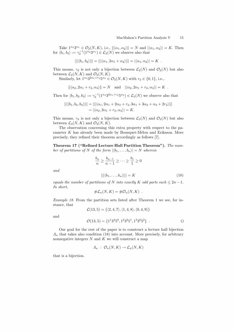
Take 1α23α1 ∈ O2(N,K), i.e., ‖〈α1, α2〉‖ = N and |〈α1, α2〉| = K. Thenfor 〈b1, b2〉 := γ−1
2 (1α23α1) ∈ L2(N) we observe also that
|||〈b1, b2〉||| = |||〈α1, 2α1 + α2〉||| = |〈α1, α2〉| = K .
This means, γ2 is not only a bijection between L2(N) and O2(N) but alsobetween L2(N,K) and O2(N,K).
Similarly, let 1α332α1+r25α2 ∈ O3(N,K) with r2 ∈ 0, 1, i.e.,
‖〈α2, 2α1 + r2, α3〉‖ = N and |〈α2, 2α1 + r2, α3〉| = K .
Then for 〈b1, b2, b3〉 := γ−13 (1α332α1+r25α2) ∈ L3(N) we observe also that
|||〈b1, b2, b3〉||| = |||〈α1, 2α1 + 2α2 + r2, 3α1 + 3α2 + α3 + 2r2〉|||= |〈α2, 2α1 + r2, α3〉| = K.
This means, γ3 is not only a bijection between L3(N) and O3(N) but alsobetween L3(N,K) and O3(N,K).
The observation concerning this extra property with respect to the pa-rameter K has already been made by Bousquet-Melou and Eriksson. Moreprecisely, they refined their theorem accordingly as follows [7].
Theorem 17 (“Refined Lecture Hall Partition Theorem”). The num-ber of partitions of N of the form |〈b1, . . . , bn〉| = N wherein
bnn≥ bn−1
n− 1≥ · · · ≥ b1
1≥ 0
and|||〈b1, . . . , bn〉||| = K (18)
equals the number of partitions of N into exactly K odd parts each ≤ 2n− 1.In short,
#Ln(N,K) = #On(N,K) .
Example 18. From the partition sets listed after Theorem 1 we see, for in-stance, that
L(13, 5) = 〈2, 4, 7〉, 〈1, 4, 8〉, 〈0, 4, 9〉
andO(13, 5) = 113450, 123251, 133052 . ut
Our goal for the rest of the paper is to construct a lecture hall bijectionΛn that takes also condition (18) into account. More precisely, for arbitrarynonnegative integers N and K we will construct a map
Λn : On(N,K)→ Ln(N,K)
that is a bijection.
16 George E. Andrews, Peter Paule, Axel Riese, and Volker Strehl
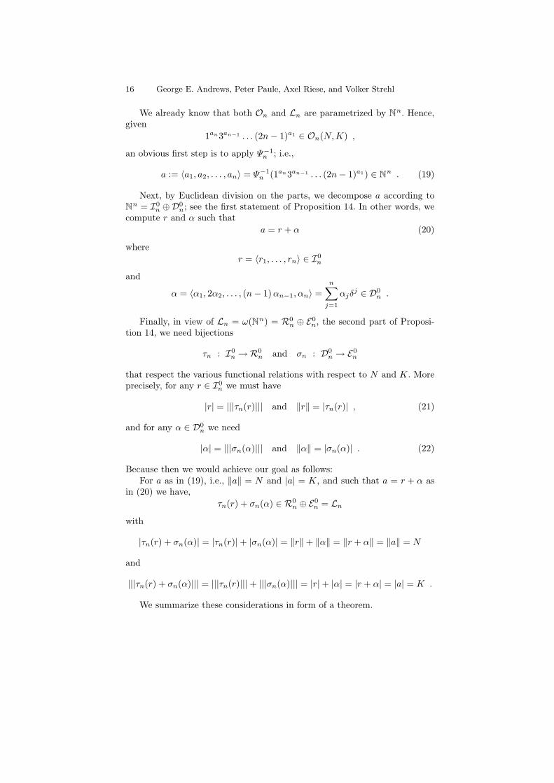
We already know that both On and Ln are parametrized by Nn. Hence,given
1an3an−1 . . . (2n− 1)a1 ∈ On(N,K) ,
an obvious first step is to apply Ψ−1n ; i.e.,
a := 〈a1, a2, . . . , an〉 = Ψ−1n (1an3an−1 . . . (2n− 1)a1) ∈ Nn . (19)
Next, by Euclidean division on the parts, we decompose a according toNn = I0
n ⊕D0n; see the first statement of Proposition 14. In other words, we
compute r and α such thata = r + α (20)
wherer = 〈r1, . . . , rn〉 ∈ I0
n
and
α = 〈α1, 2α2, . . . , (n− 1)αn−1, αn〉 =n∑j=1
αjδj ∈ D0
n .
Finally, in view of Ln = ω(Nn) = R0n ⊕ E0
n, the second part of Proposi-tion 14, we need bijections
τn : I0n → R0
n and σn : D0n → E0
n
that respect the various functional relations with respect to N and K. Moreprecisely, for any r ∈ I0
n we must have
|r| = |||τn(r)||| and ‖r‖ = |τn(r)| , (21)
and for any α ∈ D0n we need
|α| = |||σn(α)||| and ‖α‖ = |σn(α)| . (22)
Because then we would achieve our goal as follows:For a as in (19), i.e., ‖a‖ = N and |a| = K, and such that a = r + α as
in (20) we have,τn(r) + σn(α) ∈ R0
n ⊕ E0n = Ln
with
|τn(r) + σn(α)| = |τn(r)|+ |σn(α)| = ‖r‖+ ‖α‖ = ‖r + α‖ = ‖a‖ = N
and
|||τn(r) + σn(α)||| = |||τn(r)|||+ |||σn(α)||| = |r|+ |α| = |r + α| = |a| = K .
We summarize these considerations in form of a theorem.
MacMahon’s Partition Analysis V 17
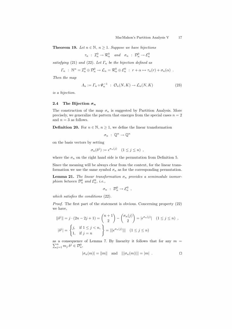
Theorem 19. Let n ∈ N, n ≥ 1. Suppose we have bijections
τn : I0n → R0
n and σn : D0n → E0
n
satisfying (21) and (22). Let Γn be the bijection defined as
Γn : Nn = I0n ⊕D0
n → Ln = R0n ⊕ E0
n : r + α 7→ τn(r) + σn(α) .
Then the map
Λn := Γn Ψ−1n : On(N,K)→ Ln(N,K) (23)
is a bijection.
2.4 The Bijection σn
The construction of the map σn is suggested by Partition Analysis. Moreprecisely, we generalize the pattern that emerges from the special cases n = 2and n = 3 as follows.
Definition 20. For n ∈ N, n ≥ 1, we define the linear transformation
σn : Qn → Qn
on the basis vectors by setting
σn(δj) := εσn(j) (1 ≤ j ≤ n) ,
where the σn on the right hand side is the permutation from Definition 5.
Since the meaning will be always clear from the context, for the linear trans-formation we use the same symbol σn as for the corresponding permutation.
Lemma 21. The linear transformation σn provides a semimodule isomor-phism between D0
n and E0n, i.e.,
σn : D0n → E0
n ,
which satisfies the conditions (22).
Proof. The first part of the statement is obvious. Concerning property (22)we have,
‖δj‖ = j · (2n− 2j + 1) =(n+ 1
2
)−(σn(j)
2
)= |εσn(j)| (1 ≤ j ≤ n) ,
|δj | =
j, if 1 ≤ j < n,
1, if j = n
= |||εσn(j)||| (1 ≤ j ≤ n)
as a consequence of Lemma 7. By linearity it follows that for any m =∑nj=1mj δ
j ∈ D0n,
|σn(m)| = ‖m‖ and |||σn(m)||| = |m| . ut
18 George E. Andrews, Peter Paule, Axel Riese, and Volker Strehl
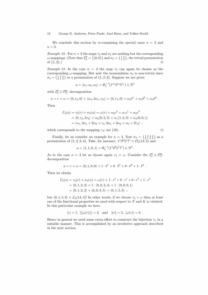
We conclude this section by re-examining the special cases n = 2 andn = 3.
Example 22. For n = 2 the maps τ2 and σ2 are nothing but the correspondingω-mappings. (Note that I0
2 = 〈0, 0〉 and σ2 =(
1 21 2
), the trivial permutation
of 1, 2.) ut
Example 23. In the case n = 3 the map τ3 can again be chosen as thecorresponding ω-mapping. But now the isomorphism σ3 is non-trivial sinceσ3 =
(1 2 32 1 3
)as a permutation of 1, 2, 3. Suppose we are given
a = 〈a1, a2, a3〉 = Ψ−13 (1a33a25a1) ∈ N3
with I03 ⊕D0
3- decomposition
a = r + α = 〈0, r2, 0〉+ 〈α2, 2α1, α3〉 = 〈0, r2, 0〉+ α2δ1 + α1δ
2 + α3δ3 .
Then
Γ3(a) = τ3(r) + σ3(α) = ω(r) + α2ε2 + α1ε
1 + α3ε3
= 〈0, r2, 2r2〉+ α2〈0, 2, 3〉+ α1〈1, 2, 3〉+ α3〈0, 0, 1〉= 〈α1, 2α1 + 2α2 + r2, 3α1 + 3α2 + α3 + 2r2〉 ,
which corresponds to the mapping γ3; see (16). ut
Finally, let us consider an example for n = 4. Now σ4 =(
1 2 3 42 1 3 4
)as a
permutation of 1, 2, 3, 4. Take, for instance, 11305171 ∈ O4(13, 3) and
a = 〈1, 1, 0, 1〉 = Ψ−14 (11305171) ∈ N4.
As in the case n = 3 let us choose again τ4 = ω. Consider the I04 ⊕ D0
4-decomposition
a = r + α = 〈0, 1, 0, 0〉+ 1 · δ1 + 0 · δ2 + 0 · δ3 + 1 · δ4 .
Then we obtain
Γ4(a) = τ4(r) + σ4(α) = ω(r) + 1 · ε3 + 0 · ε1 + 0 · ε2 + 1 · ε4
= 〈0, 1, 2, 3〉+ 1 · 〈0, 0, 3, 4〉+ 1 · 〈0, 0, 0, 1〉= 〈0, 1, 2, 3〉+ 〈0, 0, 3, 5〉 = 〈0, 1, 5, 8〉 ;
but 〈0, 1, 5, 8〉 ∈ L4(14, 4)! In other words, if we choose τ4 = ω then at leastone of the functional properties we need with respect to N and K is violated.In this particular example we have
|r| = 1, |||ω(r)||| = 2 and ‖r‖ = 5, |ω(r)| = 6 .
Hence in general we need some extra effort to construct the bijection τn in asuitable manner. This is accomplished by an involutive approach describedin the next section.
MacMahon’s Partition Analysis V 19
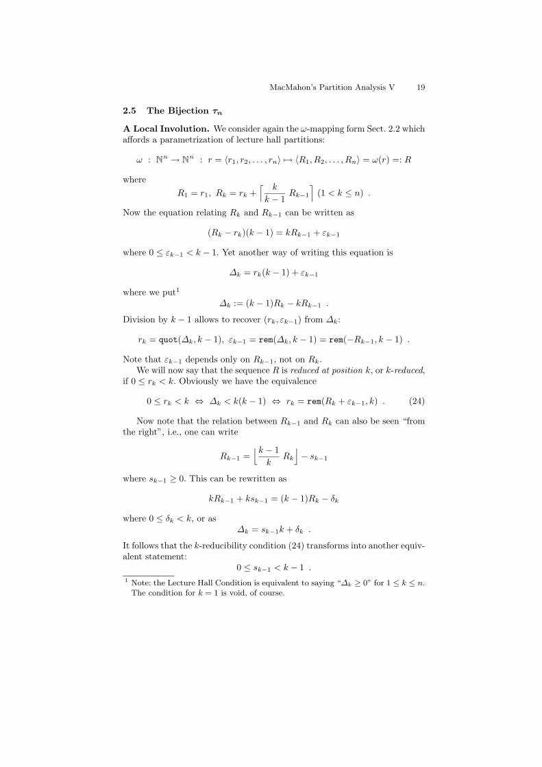
2.5 The Bijection τn
A Local Involution. We consider again the ω-mapping form Sect. 2.2 whichaffords a parametrization of lecture hall partitions:
ω : Nn → Nn : r = 〈r1, r2, . . . , rn〉 7→ 〈R1, R2, . . . , Rn〉 = ω(r) =: R
whereR1 = r1, Rk = rk +
⌈ k
k − 1Rk−1
⌉(1 < k ≤ n) .
Now the equation relating Rk and Rk−1 can be written as
(Rk − rk)(k − 1) = kRk−1 + εk−1
where 0 ≤ εk−1 < k − 1. Yet another way of writing this equation is
∆k = rk(k − 1) + εk−1
where we put1
∆k := (k − 1)Rk − kRk−1 .
Division by k − 1 allows to recover (rk, εk−1) from ∆k:
rk = quot(∆k, k − 1), εk−1 = rem(∆k, k − 1) = rem(−Rk−1, k − 1) .
Note that εk−1 depends only on Rk−1, not on Rk.We will now say that the sequence R is reduced at position k, or k-reduced,
if 0 ≤ rk < k. Obviously we have the equivalence
0 ≤ rk < k ⇔ ∆k < k(k − 1) ⇔ rk = rem(Rk + εk−1, k) . (24)
Now note that the relation between Rk−1 and Rk can also be seen “fromthe right”, i.e., one can write
Rk−1 =⌊k − 1
kRk
⌋− sk−1
where sk−1 ≥ 0. This can be rewritten as
kRk−1 + ksk−1 = (k − 1)Rk − δk
where 0 ≤ δk < k, or as∆k = sk−1k + δk .
It follows that the k-reducibility condition (24) transforms into another equiv-alent statement:
0 ≤ sk−1 < k − 1 .
1 Note: the Lecture Hall Condition is equivalent to saying “∆k ≥ 0” for 1 ≤ k ≤ n.The condition for k = 1 is void, of course.
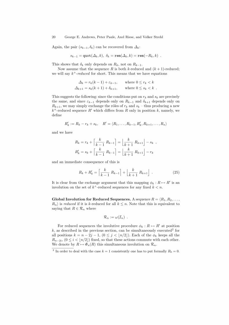
20 George E. Andrews, Peter Paule, Axel Riese, and Volker Strehl
Again, the pair (sk−1, δk) can be recovered from ∆k:
sk−1 = quot(∆k, k), δk = rem(∆k, k) = rem(−Rk, k) .
This shows that δk only depends on Rk, not on Rk−1.Now assume that the sequence R is both k-reduced and (k + 1)-reduced;
we will say k+-reduced for short. This means that we have equations
∆k = rk(k − 1) + εk−1, where 0 ≤ rk < k
∆k+1 = sk(k + 1) + δk+1, where 0 ≤ sk < k .
This suggests the following: since the conditions put on rk and sk are preciselythe same, and since εk−1 depends only on Rk−1 and δk+1 depends only onRk+1, we may simply exchange the roles of rk and sk – thus producing a newk+-reduced sequence R′ which differs from R only in position k, namely, wedefine
R′k := Rk − rk + sk, R′ = 〈R1, . . . , Rk−1, R′k, Rk+1, . . . , Rn〉
and we have
Rk = rk +⌈ k
k − 1Rk−1
⌉=⌊ k
k + 1Rk+1
⌋− sk ,
R′k = sk +⌈ k
k − 1Rk−1
⌉=⌊ k
k + 1Rk+1
⌋− rk
and an immediate consequence of this is
Rk +R′k =⌈ k
k − 1Rk−1
⌉+⌊ k
k + 1Rk+1
⌋. (25)
It is clear from the exchange argument that this mapping φk : R 7→ R′ is aninvolution on the set of k+-reduced sequences for any fixed k < n.
Global Involution for Reduced Sequences. A sequenceR = 〈R1, R2, . . . ,Rn〉 is reduced if it is k-reduced for all k ≤ n. Note that this is equivalent tosaying that R ∈ Rn where
Rn := ω(In) .
For reduced sequences the involutive procedure φk : R 7→ R′ at positionk, as described in the previous section, can be simultaneously executed2 forall positions k = n − 2j − 1, (0 ≤ j < bn/2c). Each of the φk keeps all theRn−2i, (0 ≤ i < bn/2c) fixed, so that these actions commute with each other.We denote by R 7→ Φn(R) this simultaneous involution on Rn.2 In order to deal with the case k = 1 consistently one has to put formally R0 = 0.
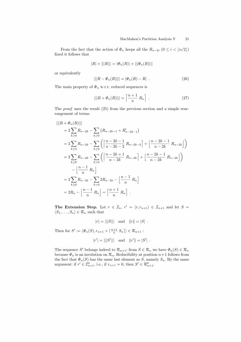
MacMahon’s Partition Analysis V 21
From the fact that the action of Φn keeps all the Rn−2i (0 ≤ i < bn/2c)fixed it follows that
|R|+ |||R||| = |Φn(R)|+ |||Φn(R)|||
or equivalently|||R− Φn(R)||| = |Φn(R)−R| . (26)
The main property of Φn w.r.t. reduced sequences is
|||R+ Φn(R)||| =⌈n+ 1
nRn
⌉. (27)
The proof uses the result (25) from the previous section and a simple rear-rangement of terms:
|||R+ Φn(R)|||
= 2∑k≥0
Rn−2k −∑k≥0
(Rn−2k−1 +R′n−2k−1
)= 2
∑k≥0
Rn−2k −∑k≥0
(⌈n− 2k − 1n− 2k − 2
Rn−2k−2
⌉+⌊n− 2k − 1
n− 2kRn−2k
⌋)
= 2∑k≥0
Rn−2k −∑k>0
(⌈n− 2k + 1n− 2k
Rn−2k
⌉+⌊n− 2k − 1
n− 2kRn−2k
⌋)−⌊n− 1
nRn
⌋= 2
∑k≥0
Rn−2k −∑k>0
2Rn−2k −⌊n− 1
nRn
⌋= 2Rn −
⌊n− 1n
Rn
⌋=⌈n+ 1
nRn
⌉.
The Extension Step. Let r ∈ In, r′ = 〈r, rn+1〉 ∈ In+1 and let S =〈S1, . . . , Sn〉 ∈ Rn such that
|r| = |||S||| and ‖r‖ = |S| .
Then for S′ := 〈Φn(S), rn+1 + dn+1n Sne〉 ∈ Rn+1 :
|r′| = |||S′||| and ‖r′‖ = |S′| .
The sequence S′ belongs indeed to Rn+1: from S ∈ Rn we have Φn(S) ∈ Rnbecause Φn is an involution on Rn. Reducibility at position n+1 follows fromthe fact that Φn(S) has the same last element as S, namely Sn. By the sameargument: if r′ ∈ I0
n+1, i.e., if rn+1 = 0, then S′ ∈ R0n+1.
22 George E. Andrews, Peter Paule, Axel Riese, and Volker Strehl
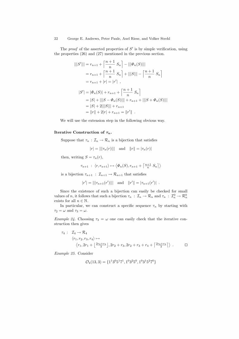
The proof of the asserted properties of S′ is by simple verification, usingthe properties (26) and (27) mentioned in the previous section.
|||S′||| = rn+1 +⌈n+ 1
nSn
⌉− |||Φn(S)|||
= rn+1 +⌈n+ 1
nSn
⌉+ |||S||| −
⌈n+ 1n
Sn
⌉= rn+1 + |r| = |r′| ,
|S′| = |Φn(S)|+ rn+1 +⌈n+ 1
nSn
⌉= |S|+ |||S − Φn(S)|||+ rn+1 + |||S + Φn(S)|||= |S|+ 2|||S|||+ rn+1
= ‖r‖+ 2|r|+ rn+1 = ‖r′‖ .
We will use the extension step in the following obvious way.
Iterative Construction of τn.
Suppose that τn : In → Rn is a bijection that satisfies
|r| = |||τn(r)||| and ‖r‖ = |τn(r)|
then, writing S = τn(r),
τn+1 : 〈r, rn+1〉 7→⟨Φn(S), rn+1 +
⌈n+1n Sn
⌉⟩is a bijection τn+1 : In+1 → Rn+1 that satisfies
|r′| = |||τn+1(r′)||| and ‖r′‖ = |τn+1(r′)| .
Since the existence of such a bijection can easily be checked for smallvalues of n, it follows that such a bijection τn : In → Rn and τn : I0
n → R0n
exists for all n ∈ N.In particular, we can construct a specific sequence τn by starting with
τ2 = ω and τ3 = ω.
Example 24. Choosing τ3 = ω one can easily check that the iterative con-struction then gives
τ4 : I4 → R4
〈r1, r2, r3, r4〉 7→⟨r1, 2r1 +
⌊2r2+r3
3
⌋, 2r2 + r3, 2r2 + r3 + r4 +
⌈2r2+r3
3
⌉⟩. ut
Example 25. Consider
O4(13, 3) = 11305171, 103250, 10315270
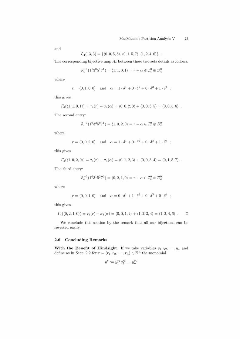
MacMahon’s Partition Analysis V 23
andL4(13, 3) = 〈0, 0, 5, 8〉, 〈0, 1, 5, 7〉, 〈1, 2, 4, 6〉 .
The corresponding bijective map Λ4 between these two sets details as follows:
Ψ−14 (11305171) = 〈1, 1, 0, 1〉 = r + α ∈ I0
4 ⊕D04
where
r = 〈0, 1, 0, 0〉 and α = 1 · δ1 + 0 · δ2 + 0 · δ3 + 1 · δ4 ;
this gives
Γ4(〈1, 1, 0, 1〉) = τ4(r) + σ4(α) = 〈0, 0, 2, 3〉+ 〈0, 0, 3, 5〉 = 〈0, 0, 5, 8〉 .
The second entry:
Ψ−14 (10325071) = 〈1, 0, 2, 0〉 = r + α ∈ I0
4 ⊕D04
where
r = 〈0, 0, 2, 0〉 and α = 1 · δ1 + 0 · δ2 + 0 · δ3 + 1 · δ4 ;
this gives
Γ4(〈1, 0, 2, 0〉) = τ4(r) + σ4(α) = 〈0, 1, 2, 3〉+ 〈0, 0, 3, 4〉 = 〈0, 1, 5, 7〉 .
The third entry:
Ψ−14 (10315270) = 〈0, 2, 1, 0〉 = r + α ∈ I0
4 ⊕D04
where
r = 〈0, 0, 1, 0〉 and α = 0 · δ1 + 1 · δ2 + 0 · δ3 + 0 · δ4 ;
this gives
Γ4(〈0, 2, 1, 0〉) = τ4(r) + σ4(α) = 〈0, 0, 1, 2〉+ 〈1, 2, 3, 4〉 = 〈1, 2, 4, 6〉 . ut
We conclude this section by the remark that all our bijections can bereverted easily.
2.6 Concluding Remarks
With the Benefit of Hindsight. If we take variables y1, y2, . . . , yn anddefine as in Sect. 2.2 for r = 〈r1, r2, . . . , rn〉 ∈ Nn the monomial
yr := yr11 yr22 · · · yrnn
24 George E. Andrews, Peter Paule, Axel Riese, and Volker Strehl
then we have from the semilinear representation of lecture hall partitions
fn(y1, y2, . . . , yn) =∑yb : b ∈ Ln = R0
n ⊕ E0n
=∑yR : R ∈ R0
n∏1≤j≤n(1− yεj )
.
Multiplying the numerator and the denominator of this last fraction by 1−yn= 1− yω(n δn) leads (thanks to a finite geometric series) to
fn(y1, y2, . . . , yn) =∑yR : R ∈ Rn∏
1≤j<n(1− yεj ) · (1− yω(n δn))
=∑yb : b ∈ Ln = Rn ⊕ En
where En = ω(Dn), and where Dn is the free semimodule generated byδ1, . . . , δn−1 and n δn = 〈0, . . . , 0, n〉(= ω(n δn)). Obviously: Nn = In ⊕ Dn.This avoids the special treatment of the last basis vector.
In other words, we could have used the semilinear presentation Ln =Rn⊕En instead of Ln = R0
n⊕E0n – and everything would have gone through
equally well. In particular, the essential properties of the mapping λn areavailable for both λn : In → Rn, and λn : I0
n → R0n.
The above use of the presentation Ln = R0n ⊕ E0
n was motivated by whatΩ-calculus (or better: its implementation) had suggested. Automatic simplifi-cation led to cancelling the factor 1−ynn , which made things less homogeneous.
Other Bijections. The involutory approach we have used for the construc-tion of τn is essentially equivalent to an involution discovered by Bousquet-Melou and Eriksson in [8, Prop. 3.4]. However, they applied this tool in adifferent direction; in addition, our presentation differs very much from thatin [8].
We also want to remark that the limiting case n → ∞ of the RefinedLecture Hall Partition Theorem (Theorem 17) finds a much more direct bi-jective treatment. In fact, before the finite version in form of Theorem 17 hadbeen discovered, in 1994 C. Bessenrodt [6, Prop. 2.2] described a very elegantbijection between the underlying sets of this limiting case. To this end Bessen-rodt uses 2-modular Young diagrams in order to formulate a new version ofa classic bijection due to Sylvester. Another variant of Sylvester’s bijectionwas given by D. Kim and A. Yee [11] in 1999; they essentially describe theinverse of Bessenrodt’s map. This gives rise to the following problem.
Problem 26. Is there any bijective proof of Theorem 17 that in the limitn→∞ converges to Bessenrodt’s bijection?
Being based on an iterative use of the involution Φn, our bijection doesnot have an infinite version. More generally one can ask the following.
MacMahon’s Partition Analysis V 25
Problem 27. Is there any bijective proof of Theorem 17 without using theinvolution Φn?
It might well be possible that there is a simpler bijection in case therefinement condition is dropped. So we conclude by raising another problem.
Problem 28. Is there any simpler lecture hall bijection for the version of The-orem 1, i.e., in case the refinement condition (18) is dropped?
Note added in proof: A.E. Yee [18] developed a bijective approach whichis different to our bijection and which seems to solve Problem 26 and Prob-lem 27.
3 Cayley Compositions
3.1 Introduction
In [9], A. Cayley poses and solves the following problem:
“It is required to find the number of [compositions] into a given num-ber of parts, such that the first part is unity, and that no part isgreater than twice the preceding part.Commencing to form the [compositions] in question, these are (readvertically):
1 1 1 1 1 1 1 1 11 2 1 1 2 2 2 2 &c. . . ”
1 2 1 2 3 4
We shall call such compositions, Cayley compositions. Let us define cj(n)to be the total number of Cayley compositions ending in n and having j parts.Thus from Cayley’s enumeration we see that c1(1) = 1, c2(1) = c2(2) = 1,c3(1) = c3(2) = 2, c3(3) = c3(4) = 1.
Clearly the Cayley composition with j parts and largest last part is1, 2, 4, . . . , 2j−1. So if we define a Cayley polynomial as
Cj(q) =∑n≥0
cj(n) qn ,
then Cj(q) has degree 2j−1. Returning to Cayley enumeration, we see that
C1(q) = q ,
C2(q) = q + q2 ,
C3(q) = 2q + 2q2 + q3 + q4 .
26 George E. Andrews, Peter Paule, Axel Riese, and Volker Strehl
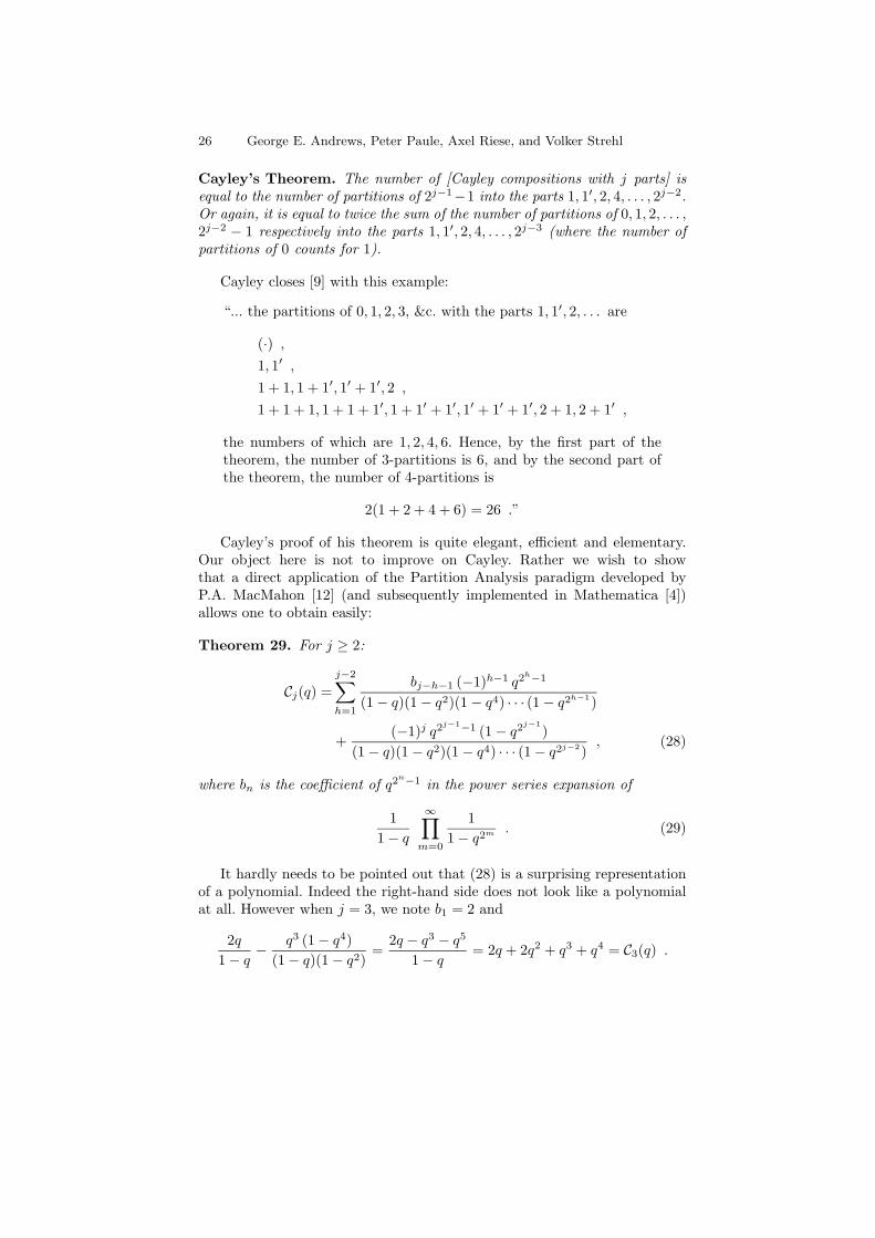
Cayley’s Theorem. The number of [Cayley compositions with j parts] isequal to the number of partitions of 2j−1−1 into the parts 1, 1′, 2, 4, . . . , 2j−2.Or again, it is equal to twice the sum of the number of partitions of 0, 1, 2, . . . ,2j−2 − 1 respectively into the parts 1, 1′, 2, 4, . . . , 2j−3 (where the number ofpartitions of 0 counts for 1).
Cayley closes [9] with this example:
“... the partitions of 0, 1, 2, 3, &c. with the parts 1, 1′, 2, . . . are
(·) ,
1, 1′ ,1 + 1, 1 + 1′, 1′ + 1′, 2 ,
1 + 1 + 1, 1 + 1 + 1′, 1 + 1′ + 1′, 1′ + 1′ + 1′, 2 + 1, 2 + 1′ ,
the numbers of which are 1, 2, 4, 6. Hence, by the first part of thetheorem, the number of 3-partitions is 6, and by the second part ofthe theorem, the number of 4-partitions is
2(1 + 2 + 4 + 6) = 26 .”
Cayley’s proof of his theorem is quite elegant, efficient and elementary.Our object here is not to improve on Cayley. Rather we wish to showthat a direct application of the Partition Analysis paradigm developed byP.A. MacMahon [12] (and subsequently implemented in Mathematica [4])allows one to obtain easily:
Theorem 29. For j ≥ 2:
Cj(q) =j−2∑h=1
bj−h−1 (−1)h−1 q2h−1
(1− q)(1− q2)(1− q4) · · · (1− q2h−1)
+(−1)j q2j−1−1 (1− q2j−1
)(1− q)(1− q2)(1− q4) · · · (1− q2j−2)
, (28)
where bn is the coefficient of q2n−1 in the power series expansion of
11− q
∞∏m=0
11− q2m
. (29)
It hardly needs to be pointed out that (28) is a surprising representationof a polynomial. Indeed the right-hand side does not look like a polynomialat all. However when j = 3, we note b1 = 2 and
2q1− q
− q3 (1− q4)(1− q)(1− q2)
=2q − q3 − q5
1− q= 2q + 2q2 + q3 + q4 = C3(q) .
MacMahon’s Partition Analysis V 27
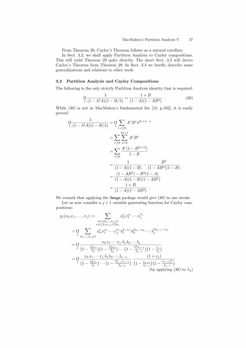
From Theorem 29, Cayley’s Theorem follows as a natural corollary.In Sect. 3.2, we shall apply Partition Analysis to Cayley compositions.
This will yield Theorem 29 quite directly. The short Sect. 3.3 will deriveCayley’s Theorem from Theorem 29. In Sect. 3.4 we briefly describe somegeneralizations and relations to other work.
3.2 Partition Analysis and Cayley Compositions
The following is the only strictly Partition Analysis identity that is required:
Ω=
λ
(1− λ2A)(1−B/λ)=
1 +B
(1−A)(1−AB2). (30)
While (30) is not in MacMahon’s fundamental list [12, p.102], it is easilyproved:
Ω=
λ
(1− λ2A)(1−B/λ)= Ω=
∑r,s≥0
ArBsλ2r+1−s
=∑r≥0
2r+1∑s=0
ArBs
=∑r≥0
Ar(1−B2r+2)1−B
=1
(1−A)(1−B)− B2
(1−AB2)(1−B)
=(1−AB2)−B2(1−A)
(1−A)(1−B)(1−AB2)
=1 +B
(1−A)(1−AB2).
We remark that applying the Omega package would give (30) in one stroke.Let us now consider a j + 1 variable generating function for Cayley com-
positions:
pj(x0,x1, . . . , xj) :=∑
n1,n2,...,nj≥1n1≤2,ni+1≤2ni
x10 x
n11 · · ·x
njj
= Ω=
∑n1,...,nj≥1
x10 x
n11 · · ·x
njj λ
2−n11 λ2n1−n2
2 · · ·λ2nj−1−njj
= Ω=
x0 x1 · · ·xj λ1λ2 · · ·λj(1− λ2
2x1
λ1
)(1− λ2
3x2
λ2
)· · ·(1− λ2
jxj−1
λj−1
)(1− xj
λj
)= Ω=
x0 x1 · · ·xj λ1λ2 · · ·λj−1(1− λ2
2x1
λ1
)· · ·(1− λ2
j−1xj−2
λj−2
) (1 + xj)(1− xj−1
λj−1
)(1− xj−1x2
j
λj−1
)(by applying (30) to λj)
28 George E. Andrews, Peter Paule, Axel Riese, and Volker Strehl
= Ω=
x0 · · ·xj λ1 · · ·λj−1(1− λ2
2x1
λ1
)· · ·(1− λ2
j−1xj−2
λj−2
) (1 + xj)(xj−1 − xj−1x2
j )
·(
xj−1
1− xj−1λj−1
−xj−1x
2j
1− xj−1x2j
λj−1
)
=xj
1− xjΩ=
x0 · · ·xj−1λ1 · · ·λj−1(1− λ2
2x1
λ1
)· · ·(1− λ2
j−1xj−2
λj−2
)( 11− xj−1
λj−1
−x2j
1− xj−1x2j
λj−1
)=
xj1− xj
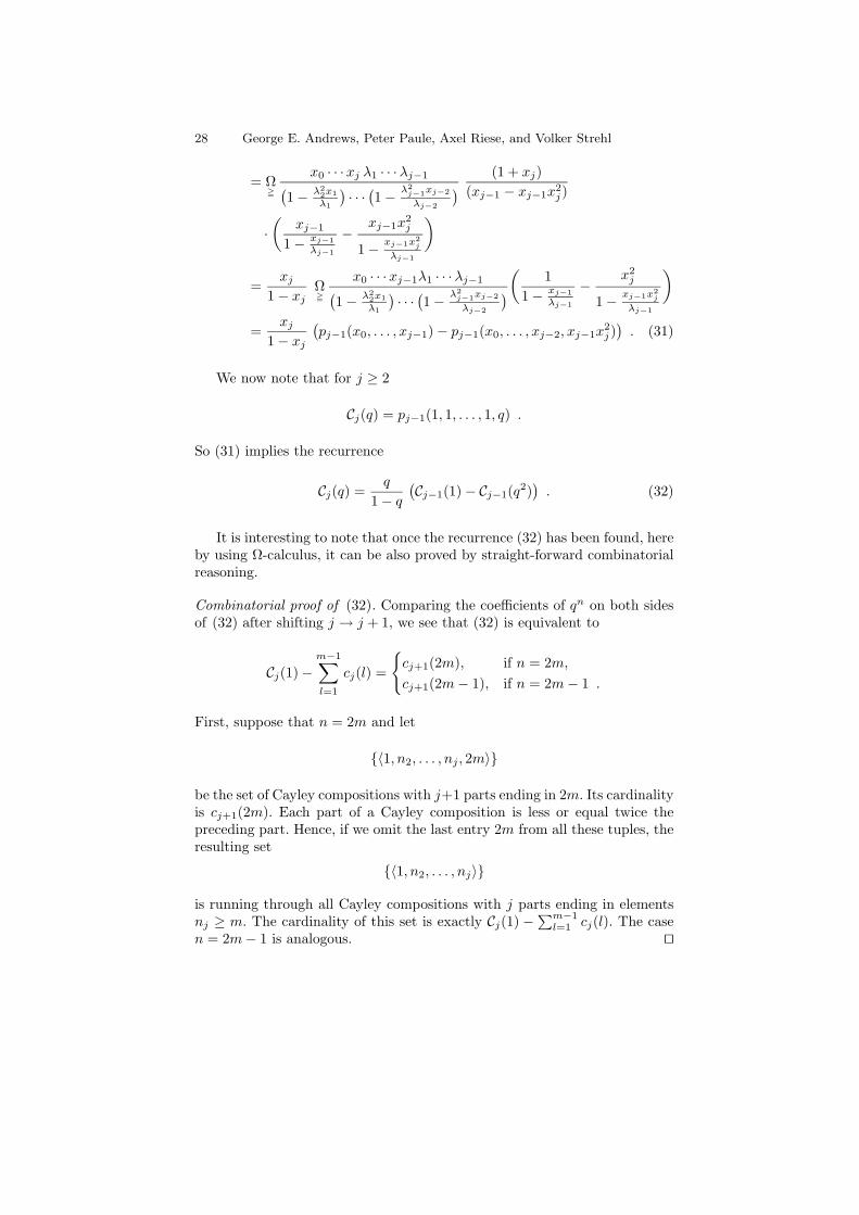
(pj−1(x0, . . . , xj−1)− pj−1(x0, . . . , xj−2, xj−1x
2j )). (31)
We now note that for j ≥ 2
Cj(q) = pj−1(1, 1, . . . , 1, q) .
So (31) implies the recurrence
Cj(q) =q
1− q(Cj−1(1)− Cj−1(q2)
). (32)
It is interesting to note that once the recurrence (32) has been found, hereby using Ω-calculus, it can be also proved by straight-forward combinatorialreasoning.
Combinatorial proof of (32). Comparing the coefficients of qn on both sidesof (32) after shifting j → j + 1, we see that (32) is equivalent to
Cj(1)−m−1∑l=1
cj(l) =
cj+1(2m), if n = 2m,cj+1(2m− 1), if n = 2m− 1 .
First, suppose that n = 2m and let
〈1, n2, . . . , nj , 2m〉
be the set of Cayley compositions with j+1 parts ending in 2m. Its cardinalityis cj+1(2m). Each part of a Cayley composition is less or equal twice thepreceding part. Hence, if we omit the last entry 2m from all these tuples, theresulting set
〈1, n2, . . . , nj〉
is running through all Cayley compositions with j parts ending in elementsnj ≥ m. The cardinality of this set is exactly Cj(1) −
∑m−1l=1 cj(l). The case
n = 2m− 1 is analogous. ut
MacMahon’s Partition Analysis V 29
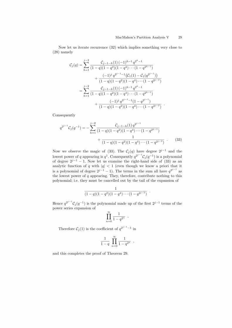
Now let us iterate recurrence (32) which implies something very close to(28) namely
Cj(q) =j−2∑h=1
Cj−1−h(1) (−1)h−1 q2h−1
(1− q)(1− q2)(1− q4) · · · (1− q2h−1)
+(−1)j q2j−1−1
(C1(1)− C1(q2j−1
))
(1− q)(1− q2)(1− q4) · · · (1− q2j−2)
=j−2∑h=1
Cj−1−h(1) (−1)h−1 q2h−1
(1− q)(1− q2)(1− q4) · · · (1− q2h−1)
+(−1)j q2j−1−1(1− q2j−1
)(1− q)(1− q2)(1− q4) · · · (1− q2j−2)
.
Consequently
q2j−1Cj(q−1) = −
j−2∑h=1
Cj−1−h(1) q2j−1
(1− q)(1− q2)(1− q4) · · · (1− q2h−1)
+1
(1− q)(1− q2)(1− q4) · · · (1− q2j−2). (33)
Now we observe the magic of (33). The Cj(q) have degree 2j−1 and thelowest power of q appearing is q1. Consequently q2j−1Cj(q−1) is a polynomialof degree 2j−1 − 1. Now let us examine the right-hand side of (33) as ananalytic function of q with |q| < 1 (even though we know a priori that itis a polynomial of degree 2j−1 − 1). The terms in the sum all have q2j−1
asthe lowest power of q appearing. They, therefore, contribute nothing to thispolynomial; i.e. they must be cancelled out by the tail of the expansion of
1(1− q)(1− q2)(1− q4) · · · (1− q2j−2)
.
Hence q2j−1Cj(q−1) is the polynomial made up of the first 2j−1 terms of thepower series expansion of
∞∏n=0
11− q2n
.
Therefore Cj(1) is the coefficient of q2j−1−1 in
11− q
∞∏n=0
11− q2n
,
and this completes the proof of Theorem 29.
30 George E. Andrews, Peter Paule, Axel Riese, and Volker Strehl
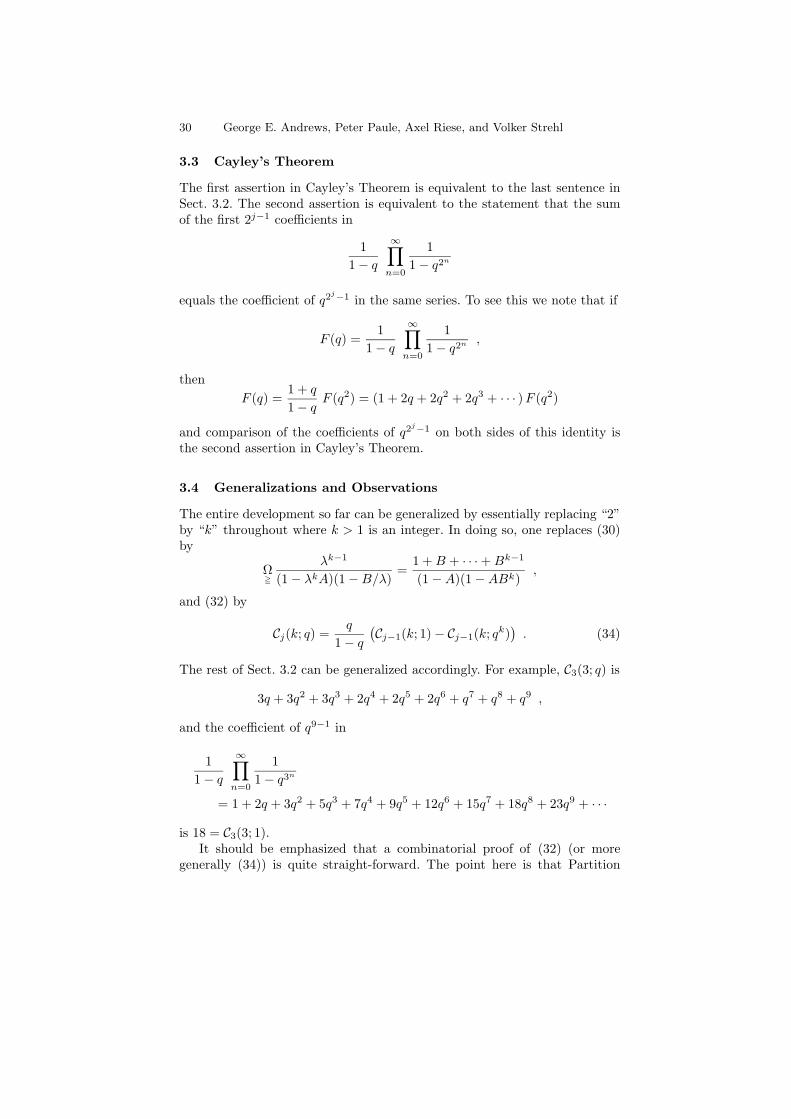
3.3 Cayley’s Theorem
The first assertion in Cayley’s Theorem is equivalent to the last sentence inSect. 3.2. The second assertion is equivalent to the statement that the sumof the first 2j−1 coefficients in
11− q
∞∏n=0
11− q2n
equals the coefficient of q2j−1 in the same series. To see this we note that if
F (q) =1
1− q
∞∏n=0
11− q2n
,
thenF (q) =
1 + q
1− qF (q2) = (1 + 2q + 2q2 + 2q3 + · · · )F (q2)
and comparison of the coefficients of q2j−1 on both sides of this identity isthe second assertion in Cayley’s Theorem.
3.4 Generalizations and Observations
The entire development so far can be generalized by essentially replacing “2”by “k” throughout where k > 1 is an integer. In doing so, one replaces (30)by
Ω=
λk−1
(1− λkA)(1−B/λ)=
1 +B + · · ·+Bk−1
(1−A)(1−ABk),
and (32) by
Cj(k; q) =q
1− q(Cj−1(k; 1)− Cj−1(k; qk)
). (34)
The rest of Sect. 3.2 can be generalized accordingly. For example, C3(3; q) is
3q + 3q2 + 3q3 + 2q4 + 2q5 + 2q6 + q7 + q8 + q9 ,
and the coefficient of q9−1 in
11− q
∞∏n=0
11− q3n
= 1 + 2q + 3q2 + 5q3 + 7q4 + 9q5 + 12q6 + 15q7 + 18q8 + 23q9 + · · ·
is 18 = C3(3; 1).It should be emphasized that a combinatorial proof of (32) (or more
generally (34)) is quite straight-forward. The point here is that Partition
MacMahon’s Partition Analysis V 31
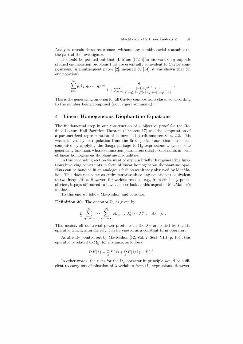
Analysis reveals these recurrences without any combinatorial reasoning onthe part of the investigator.
It should be pointed out that H. Minc [13,14] in his work on groupoidsstudied enumeration problems that are essentially equivalent to Cayley com-positions. In a subsequent paper [2], inspired by [14], it was shown that (inour notation)
∞∑j=0
pj(q, q, . . . , q) =q
1 +∑∞j=1
(−1)j q2j+1−j−1
(1−q)(1−q3)(1−q7)···(1−q2j−1)
.
This is the generating function for all Cayley compositions classified accordingto the number being composed (not largest summand).
4 Linear Homogeneous Diophantine Equations
The fundamental step in our construction of a bijective proof for the Re-fined Lecture Hall Partition Theorem (Theorem 17) was the computation ofa parametrized representation of lecture hall partitions; see Sect. 2.2. Thiswas achieved by extrapolation from the first special cases that have beencomputed by applying the Omega package to Ω=-expressions which encodegenerating functions whose summation parameters satisfy constraints in formof linear homogeneous diophantine inequalities.
In this concluding section we want to explain briefly that generating func-tions involving constraints in form of linear homogeneous diophantine equa-tions can be handled in an analogous fashion as already observed by MacMa-hon. This does not come as entire surprise since any equation is equivalentto two inequalities. However, for various reasons, e.g., from efficiency point-of-view, it pays off indeed to have a closer look at this aspect of MacMahon’smethod.
To this end we follow MacMahon and consider:
Definition 30. The operator Ω= is given by
Ω=
∞∑s1=−∞
· · ·∞∑
sr=−∞As1,...,srλ
s11 · · ·λsrr := A0,...,0 .
This means, all nontrivial power-products in the λ’s are killed by the Ω=
operator which, alternatively, can be viewed as a constant term operator.
As already pointed out by MacMahon [12, Vol. 2, Sect. VIII, p. 104], thisoperator is related to Ω=, for instance, as follows:
Ω=F (λ) = Ω
=F (λ) + Ω
=F (1/λ)− F (1) .
In other words, the rules for the Ω= operator in principle would be suffi-cient to carry out elimination of λ-variables from Ω=-expressions. However,
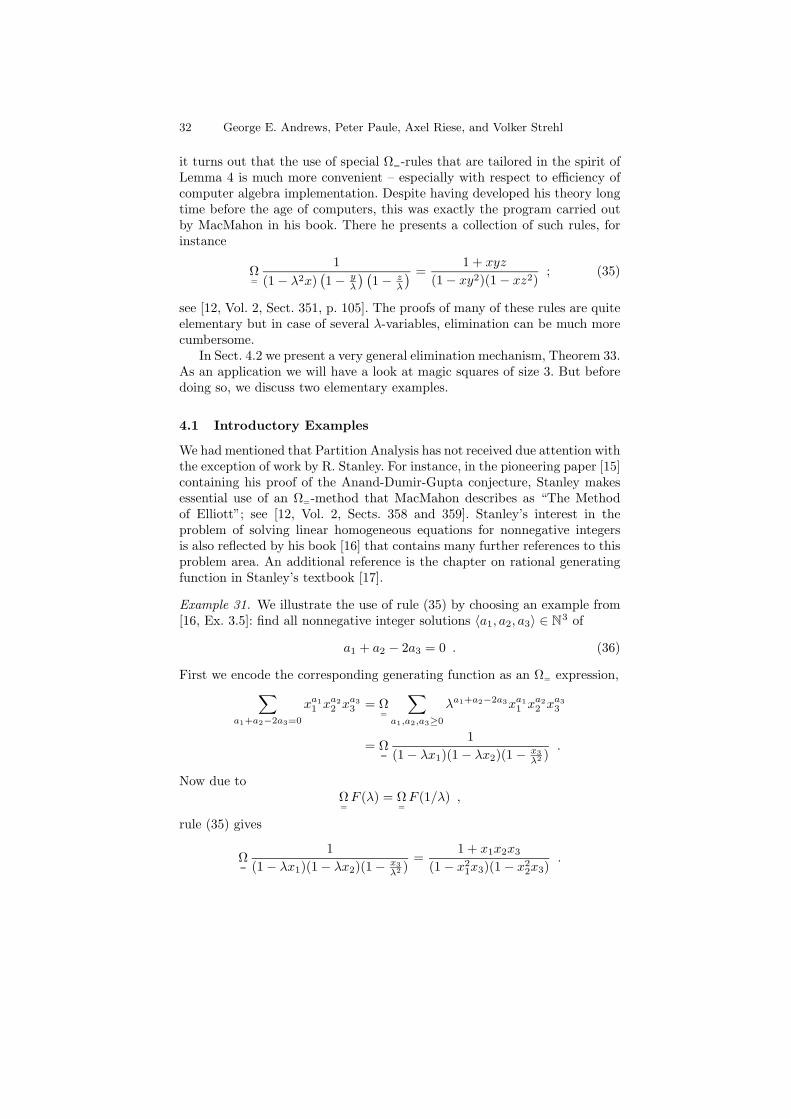
32 George E. Andrews, Peter Paule, Axel Riese, and Volker Strehl
it turns out that the use of special Ω=-rules that are tailored in the spirit ofLemma 4 is much more convenient – especially with respect to efficiency ofcomputer algebra implementation. Despite having developed his theory longtime before the age of computers, this was exactly the program carried outby MacMahon in his book. There he presents a collection of such rules, forinstance
Ω=
1(1− λ2x)
(1− y
λ
) (1− z
λ
) =1 + xyz
(1− xy2)(1− xz2); (35)
see [12, Vol. 2, Sect. 351, p. 105]. The proofs of many of these rules are quiteelementary but in case of several λ-variables, elimination can be much morecumbersome.
In Sect. 4.2 we present a very general elimination mechanism, Theorem 33.As an application we will have a look at magic squares of size 3. But beforedoing so, we discuss two elementary examples.
4.1 Introductory Examples
We had mentioned that Partition Analysis has not received due attention withthe exception of work by R. Stanley. For instance, in the pioneering paper [15]containing his proof of the Anand-Dumir-Gupta conjecture, Stanley makesessential use of an Ω=-method that MacMahon describes as “The Methodof Elliott”; see [12, Vol. 2, Sects. 358 and 359]. Stanley’s interest in theproblem of solving linear homogeneous equations for nonnegative integersis also reflected by his book [16] that contains many further references to thisproblem area. An additional reference is the chapter on rational generatingfunction in Stanley’s textbook [17].
Example 31. We illustrate the use of rule (35) by choosing an example from[16, Ex. 3.5]: find all nonnegative integer solutions 〈a1, a2, a3〉 ∈ N3 of
a1 + a2 − 2a3 = 0 . (36)
First we encode the corresponding generating function as an Ω= expression,∑a1+a2−2a3=0
xa11 xa2
2 xa33 = Ω
=
∑a1,a2,a3≥0
λa1+a2−2a3xa11 xa2
2 xa33
= Ω=
1(1− λx1)(1− λx2)(1− x3
λ2 ).
Now due toΩ=F (λ) = Ω
=F (1/λ) ,
rule (35) gives
Ω=
1(1− λx1)(1− λx2)(1− x3
λ2 )=
1 + x1x2x3
(1− x21x3)(1− x2
2x3).
MacMahon’s Partition Analysis V 33
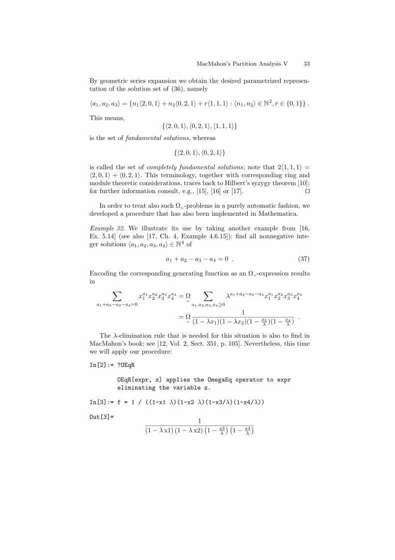
By geometric series expansion we obtain the desired parametrized represen-tation of the solution set of (36), namely
〈a1, a2, a3〉 = n1〈2, 0, 1〉+ n2〈0, 2, 1〉+ r〈1, 1, 1〉 : 〈n1, n2〉 ∈ N2, r ∈ 0, 1 .
This means,〈2, 0, 1〉, 〈0, 2, 1〉, 〈1, 1, 1〉
is the set of fundamental solutions, whereas
〈2, 0, 1〉, 〈0, 2, 1〉
is called the set of completely fundamental solutions; note that 2〈1, 1, 1〉 =〈2, 0, 1〉 + 〈0, 2, 1〉. This terminology, together with corresponding ring andmodule theoretic considerations, traces back to Hilbert’s syzygy theorem [10];for further information consult, e.g., [15], [16] or [17]. ut
In order to treat also such Ω=-problems in a purely automatic fashion, wedeveloped a procedure that has also been implemented in Mathematica.
Example 32. We illustrate its use by taking another example from [16,Ex. 5.14] (see also [17, Ch. 4, Example 4.6.15]): find all nonnegative inte-ger solutions 〈a1, a2, a3, a4〉 ∈ N4 of
a1 + a2 − a3 − a4 = 0 . (37)
Encoding the corresponding generating function as an Ω=-expression resultsin ∑
a1+a2−a3−a4=0
xa11 xa2
2 xa33 xa4
4 = Ω=
∑a1,a2,a3,a4≥0
λa1+a2−a3−a4xa11 xa2
2 xa33 xa4
4
= Ω=
1(1− λx1)(1− λx2)(1− x3
λ )(1− x4λ )
.
The λ-elimination rule that is needed for this situation is also to find inMacMahon’s book; see [12, Vol. 2, Sect. 351, p. 105]. Nevertheless, this timewe will apply our procedure:
In[2]:= ?OEqR
OEqR[expr, z] applies the OmegaEq operator to expreliminating the variable z.
In[3]:= f = 1 / ((1-x1 λ)(1-x2 λ)(1-x3/λ)(1-x4/λ))
Out[3]=1
(1− λ x1) (1− λ x2)(1− x3
λ
) (1− x4
λ
)
34 George E. Andrews, Peter Paule, Axel Riese, and Volker Strehl
In[4]:= OEqR[f, λ]
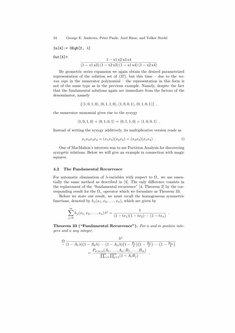
Out[4]=1− x1 x2 x3 x4
(1− x1 x3) (1− x2 x3) (1− x1 x4) (1− x2 x4)
By geometric series expansion we again obtain the desired parametrizedrepresentation of the solution set of (37), but this time – due to the mi-nus sign in the numerator polynomial – the representation in this form isnot of the same type as in the previous example. Namely, despite the factthat the fundamental solutions again are immediate from the factors of thedenominator, namely
〈1, 0, 1, 0〉, 〈0, 1, 1, 0〉, 〈1, 0, 0, 1〉, 〈0, 1, 0, 1〉 ,
the numerator monomial gives rise to the syzygy
〈1, 0, 1, 0〉+ 〈0, 1, 0, 1〉 = 〈0, 1, 1, 0〉+ 〈1, 0, 0, 1〉 .
Instead of writing the syzygy additively, its multiplicative version reads as
x1x2x3x4 = (x1x3)(x2x4) = (x2x3)(x1x4) . ut
One of MacMahon’s interests was to use Partition Analysis for discoveringsyzygetic relations. Below we will give an example in connection with magicsquares.
4.2 The Fundamental Recurrence
For automatic elimination of λ-variables with respect to Ω= we use essen-tially the same method as described in [4]. The only difference consists inthe replacement of the “fundamental recurrence” [4, Theorem 2] by the cor-responding result for the Ω= operator which we formulate as Theorem 33.
Before we state our result, we must recall the homogeneous symmetricfunctions, denoted by hj(x1, x2, . . . , xn), which are given by
∞∑j=0
hj(x1, x2, . . . , xn) tj =1
(1− tx1)(1− tx2) · · · (1− txn).
Theorem 33 (“Fundamental Recurrence”). For n and m positive inte-gers and a any integer,
Ω=
λa
(1−A1λ)(1−A2λ) · · · (1−Anλ)(1− B1
λ
)(1− B2
λ
)· · ·(1− Bm
λ
)=Pn,m,a(A1, . . . , An;B1, . . . , Bm)∏n
i=1
∏mj=1(1−AiBj)
,
MacMahon’s Partition Analysis V 35
where for n > 1,
Pn,m,a(A1, . . . , An;B1, . . . , Bm)
=1
An −An−1
·An
m∏j=1
(1−An−1Bj)Pn−1,m,a(A1, . . . , An−2, An;B1, . . . , Bm)
−An−1
m∏j=1
(1−AnBj)Pn−1,m,a(A1, . . . , An−2, An−1;B1, . . . , Bm)
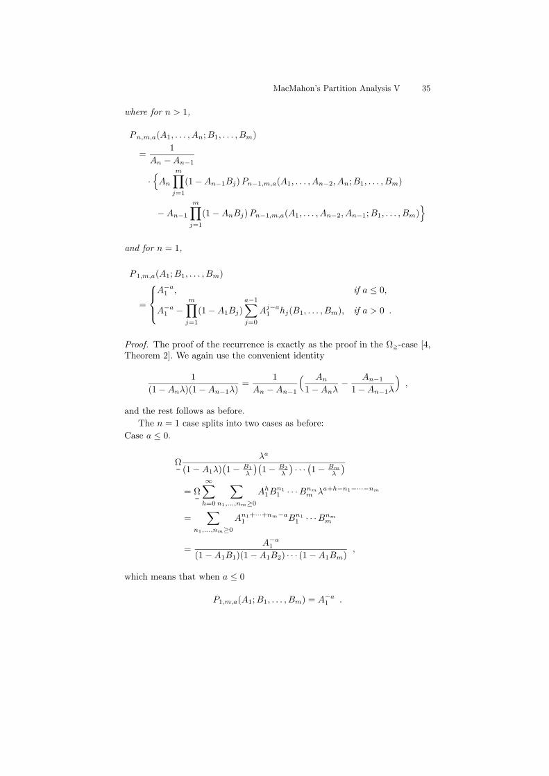
and for n = 1,
P 1,m,a(A1;B1, . . . , Bm)
=
A−a1 , if a ≤ 0,
A−a1 −m∏j=1
(1−A1Bj)a−1∑j=0
Aj−a1 hj(B1, . . . , Bm), if a > 0 .
Proof. The proof of the recurrence is exactly as the proof in the Ω=-case [4,Theorem 2]. We again use the convenient identity
1(1−Anλ)(1−An−1λ)
=1
An −An−1
( An1−Anλ
− An−1
1−An−1λ
),
and the rest follows as before.The n = 1 case splits into two cases as before:
Case a ≤ 0.
Ω=
λa
(1−A1λ)(1− B1
λ
)(1− B2
λ
)· · ·(1− Bm
λ
)= Ω
=
∞∑h=0
∑n1,...,nm≥0
Ah1Bn11 · · ·Bnmm λa+h−n1−···−nm
=∑
n1,...,nm≥0
An1+···+nm−a1 Bn1
1 · · ·Bnmm
=A−a1
(1−A1B1)(1−A1B2) · · · (1−A1Bm),
which means that when a ≤ 0
P1,m,a(A1;B1, . . . , Bm) = A−a1 .
36 George E. Andrews, Peter Paule, Axel Riese, and Volker Strehl
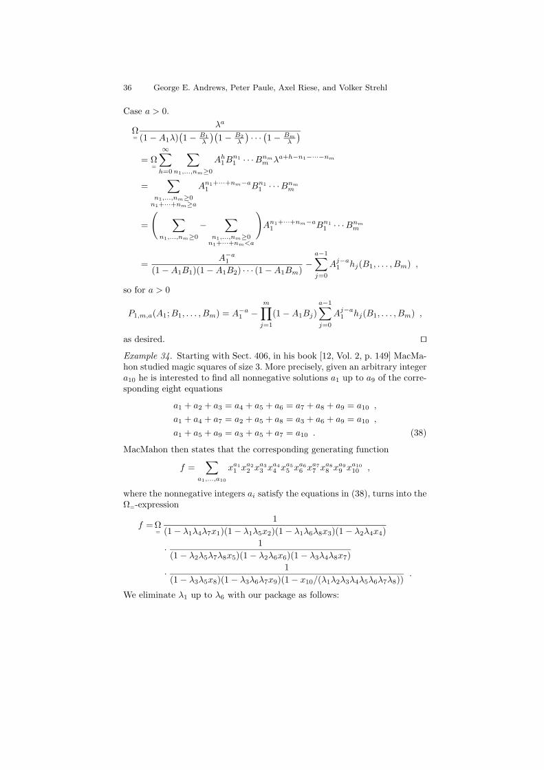
Case a > 0.
Ω=
λa
(1−A1λ)(1− B1
λ
)(1− B2
λ
)· · ·(1− Bm
λ
)= Ω
=
∞∑h=0
∑n1,...,nm≥0
Ah1Bn11 · · ·Bnmm λa+h−n1−···−nm
=∑
n1,...,nm≥0n1+···+nm≥a
An1+···+nm−a1 Bn1
1 · · ·Bnmm
=
( ∑n1,...,nm≥0
−∑
n1,...,nm≥0n1+···+nm<a
)An1+···+nm−a
1 Bn11 · · ·Bnmm
=A−a1
(1−A1B1)(1−A1B2) · · · (1−A1Bm)−a−1∑j=0
Aj−a1 hj(B1, . . . , Bm) ,
so for a > 0
P1,m,a(A1;B1, . . . , Bm) = A−a1 −m∏j=1
(1−A1Bj)a−1∑j=0
Aj−a1 hj(B1, . . . , Bm) ,
as desired. ut
Example 34. Starting with Sect. 406, in his book [12, Vol. 2, p. 149] MacMa-hon studied magic squares of size 3. More precisely, given an arbitrary integera10 he is interested to find all nonnegative solutions a1 up to a9 of the corre-sponding eight equations
a1 + a2 + a3 = a4 + a5 + a6 = a7 + a8 + a9 = a10 ,
a1 + a4 + a7 = a2 + a5 + a8 = a3 + a6 + a9 = a10 ,
a1 + a5 + a9 = a3 + a5 + a7 = a10 . (38)
MacMahon then states that the corresponding generating function
f =∑
a1,...,a10
xa11 xa2
2 xa33 xa4
4 xa55 xa6
6 xa77 xa8
8 xa99 xa10
10 ,
where the nonnegative integers ai satisfy the equations in (38), turns into theΩ=-expression
f = Ω=
1(1− λ1λ4λ7x1)(1− λ1λ5x2)(1− λ1λ6λ8x3)(1− λ2λ4x4)
· 1(1− λ2λ5λ7λ8x5)(1− λ2λ6x6)(1− λ3λ4λ8x7)
· 1(1− λ3λ5x8)(1− λ3λ6λ7x9)(1− x10/(λ1λ2λ3λ4λ5λ6λ7λ8))
.
We eliminate λ1 up to λ6 with our package as follows:
MacMahon’s Partition Analysis V 37
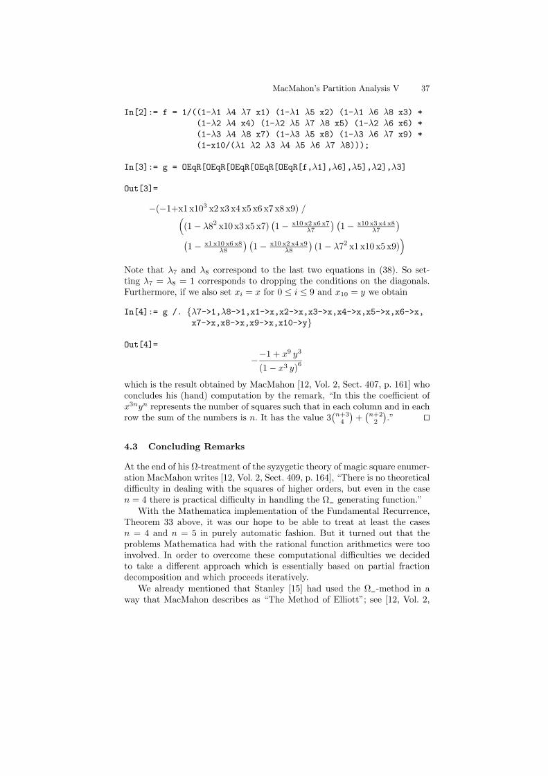
In[2]:= f = 1/((1-λ1 λ4 λ7 x1) (1-λ1 λ5 x2) (1-λ1 λ6 λ8 x3) *(1-λ2 λ4 x4) (1-λ2 λ5 λ7 λ8 x5) (1-λ2 λ6 x6) *(1-λ3 λ4 λ8 x7) (1-λ3 λ5 x8) (1-λ3 λ6 λ7 x9) *(1-x10/(λ1 λ2 λ3 λ4 λ5 λ6 λ7 λ8)));
In[3]:= g = OEqR[OEqR[OEqR[OEqR[OEqR[f,λ1],λ6],λ5],λ2],λ3]
Out[3]=
−(−1+x1 x103 x2 x3 x4 x5 x6 x7 x8 x9) /((1− λ82 x10 x3 x5 x7)
(1− x10 x2 x6 x7
λ7
) (1− x10 x3 x4 x8
λ7
)(1− x1 x10 x6 x8
λ8
) (1− x10 x2 x4 x9
λ8
)(1− λ72 x1 x10 x5 x9)
)Note that λ7 and λ8 correspond to the last two equations in (38). So set-ting λ7 = λ8 = 1 corresponds to dropping the conditions on the diagonals.Furthermore, if we also set xi = x for 0 ≤ i ≤ 9 and x10 = y we obtain
In[4]:= g /. λ7->1,λ8->1,x1->x,x2->x,x3->x,x4->x,x5->x,x6->x,x7->x,x8->x,x9->x,x10->y
Out[4]=
−−1 + x9 y3
(1− x3 y)6
which is the result obtained by MacMahon [12, Vol. 2, Sect. 407, p. 161] whoconcludes his (hand) computation by the remark, “In this the coefficient ofx3nyn represents the number of squares such that in each column and in eachrow the sum of the numbers is n. It has the value 3
(n+3
4
)+(n+2
2
).” ut
4.3 Concluding Remarks
At the end of his Ω-treatment of the syzygetic theory of magic square enumer-ation MacMahon writes [12, Vol. 2, Sect. 409, p. 164], “There is no theoreticaldifficulty in dealing with the squares of higher orders, but even in the casen = 4 there is practical difficulty in handling the Ω= generating function.”
With the Mathematica implementation of the Fundamental Recurrence,Theorem 33 above, it was our hope to be able to treat at least the casesn = 4 and n = 5 in purely automatic fashion. But it turned out that theproblems Mathematica had with the rational function arithmetics were tooinvolved. In order to overcome these computational difficulties we decidedto take a different approach which is essentially based on partial fractiondecomposition and which proceeds iteratively.
We already mentioned that Stanley [15] had used the Ω=-method in away that MacMahon describes as “The Method of Elliott”; see [12, Vol. 2,
38 George E. Andrews, Peter Paule, Axel Riese, and Volker Strehl
Sects. 358 and 359]. Also this algorithm proceeds iteratively with basic stepsbeing partial fraction decompositions of the type
1(1− xλA)(1− y
λB)
=1
1− xyλA−B
(1
1− xλA+
11− y
λB− 1)
,
where A and B are positive integers.Our new Ω=-algorithm [5] is a variation of this Elliott iteration but uses
a different partial fraction decomposition for the fundamental steps. Com-putations show that concerning efficiency this new strategy is far superiorto the method of Elliott and also considerably faster than the implementa-tion based on the Fundamental Recurrence. Moreover, we adapted this newmethod also to the Ω=-situation where we achieved a similar speed-up. Fi-nally we want to mention that using this new approach the computation ofthe generating function for general magic squares of order 4 has been reducedto a basic problem of computer algebra, namely to the task of adding 254rational functions, i.e., to simplify them to a single one. So far we were notable to accomplish this in Mathematica.
References
1. G.E. Andrews, The Theory of Partitions, Encyclopedia of Mathematics and ItsApplications, Vol. 2, G.-C. Rota ed., Addison-Wesley, Reading, 1976. (Reissued:Cambridge University Press, Cambridge, 1985.)
2. G.E. Andrews, The Rogers-Ramanujan reciprocal and Minc’s partition func-tion, Pacific J. Math. 95 (1981), 251–256.
3. G.E. Andrews, MacMahon’s partition analysis I: The lecture hall partition the-orem, in “Mathematical essays in honor of Gian-Carlo Rota’s 65th birthday”(B.E. Sagan et al., eds.), Prog. Math. 161, Birkhauser, Boston, 1998, pp. 1–22.
4. G.E. Andrews, P. Paule and A. Riese, MacMahon’s partition analysis III: TheOmega package, (to appear).
5. G.E. Andrews, P. Paule and A. Riese, MacMahon’s partition analysis VI: Thefast algorithm, (in preparation).
6. C. Bessenrodt, A bijection for Lebesgue’s identity in the spirit of Sylvester,Discrete Math. 132 (1994), 1–10.
7. M. Bousquet-Melou and K. Eriksson, Lecture hall partitions, Ramanujan J. 1(1997), 101–111.
8. M. Bousquet-Melou and K. Eriksson, Lecture hall partitions II, Ramanujan J. 1(1997), 165–187.
9. A. Cayley, On a problem in the partition of numbers, Philosophical Mag. 13(1857), 245–248 (reprinted: The Coll. Math. Papers of A. Cayley, Vol. III,Cambridge University Press, Cambridge, 1890, pp. 247–249).
10. D. Hilbert, Uber die Theorie der algebraischen Formen, Math. Ann. 36 (1890),473–534.
11. D. Kim and A.J. Yee, A note on partitions into distinct parts and odd parts,Ramanujan J. 3 (1999), 227–231.
12. P.A. MacMahon, Combinatory Analysis, 2 vols., Cambridge University Press,Cambridge, 1915–16 (reprinted: Chelsea, New York, 1960).
MacMahon’s Partition Analysis V 39
13. H. Minc, The free commutative entropic logarithmetic, Proc. Roy. Soc. Edin-burgh 65 (1959), 177–192.
14. H. Minc, A problem in partitions: Enumeration of elements of a given degree inthe free commutative entropic groupoid, Proc. Edinburgh Math. Soc. 11 (1959),223–224.
15. R.P. Stanley, Linear homogeneous diophantine equations and magic labelings ofgraphs, Duke Math. J. 40 (1973), 607–632.
16. R.P. Stanley, Combinatorics and Commutative Algebra, Birkhauser, Boston,1983.
17. R.P. Stanley, Enumerative Combinatorics - Volume 1, Wadsworth, Monterey,California, 1986.
18. A.J. Yee, On Combinatorics of Lecture Hall Partitions, (to appear).