Machine Vision FundamentalsThe Background

EMVAGran Vía de Carles III 8408028 Barcelona, SPAINinfo@emva.orgwww.emva.org

IMAGE PROCESSING in industrial appli-cations is often much simplified when the lighting device provides an image with a homogeneous background. Such a situa-tion allows for robust, stable segmentation of foreground and background. This article deals with some simple methods of image processing which may be useful for the evaluation of certain features of a lighting solution.

Distribution of grey levels

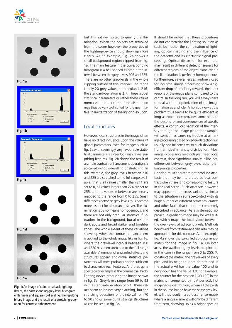
The purpose of lighting in industrial image processing is to enhance the relevant fea-tures of objects and to mask those prop-erties that are of no importance or might even produce unwanted effects. The sim-plest case would be a lighting device that produces a near binary image with clear contrast between objects and background. Fig. 1a shows a typical example. Most ap-plication engineers are quite satisfied when the grey-level image can be transformed into a proper binary image by means of a single global threshold that may be chosen from a broad interval without producing significant deterioration of the segmentation. Such a situation is usually evaluated by analysis of the grey-level histogram. Fig. 1b shows the histogram for fig. 1a. This is a nice example of a bimodal distribution with two clearly separated features. One cluster around grey-level 25 belongs to the pixels of the dark objects, while the other cluster around grey-level 215 is formed by the pixels in the

background. Global thresholding with the grey-level 104 results in the binary image in fig. 1d with clear segmentation of objects and background.

We thus seem to look at an ideal lighting so-lution. In detail, however, the situation turns out to be a bit more complicated. Since fig. 1a shows several coins placed on a backlight-device, the histogram should feature just two sharp lines corresponding to the dark coins and the bright background. What we ob-serve, however, are two clusters with a width of about 20 grey-levels. Fig. 1c reveals even more structure in the grey-level distribution. The ordinate shows the square-root of the number of pixels with the corresponding grey-level rather than the number itself as in fig. 1b. This representation shows that for every grey-level between the two prominent clusters, at least some pixels can be found in the image. One reason for the appearance of these grey-levels is the special situation at the edge of the coins, where reflection, shadows and the optical properties of the lens contribute to a continuous intensity profile of the edge, which is sampled by the discrete grid of the detector in the image-plane of the camera. Signal noise as well as differences in sensitivity from pixel to pixel and the variation of the dark signal (“fixed pattern noise”) also contribute to the scatter of the grey-levels.

The grey-level distribution of an image with objects on a background is a useful tool for the evaluation of the general situation,

Machine Vision Fundamentals The Background EMVA 01/2017 | 1

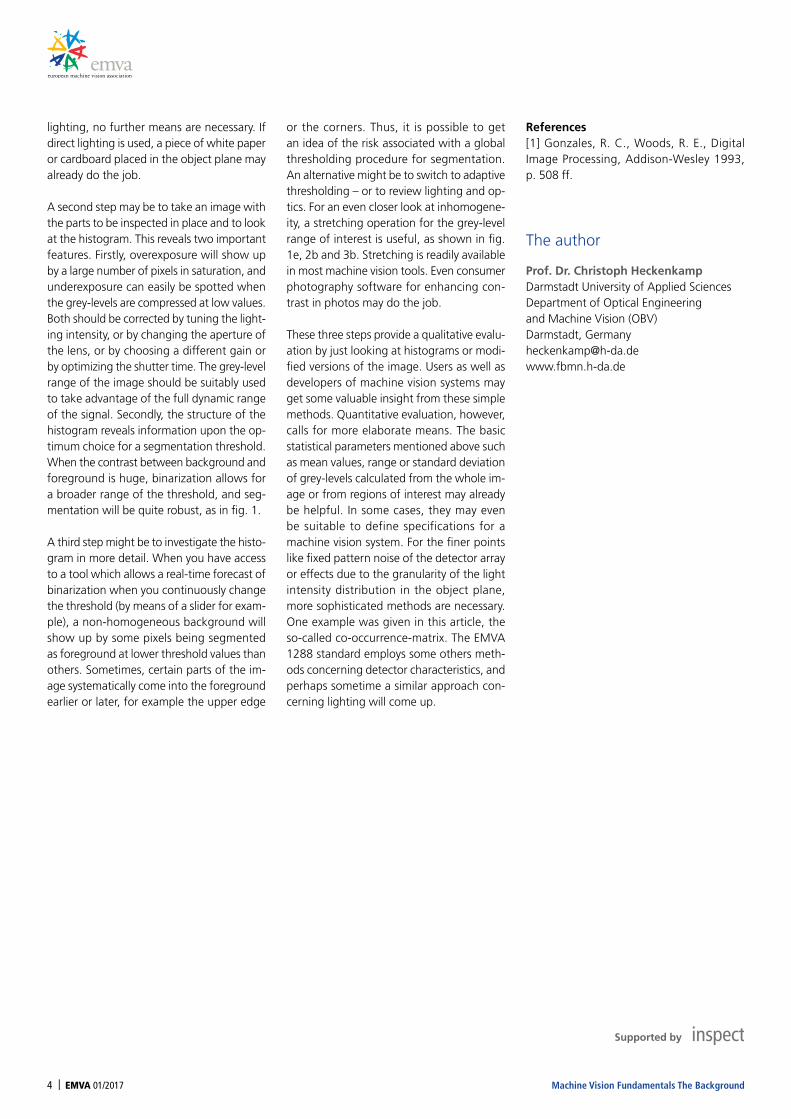
but it is not well suited to qualify the illu-mination. When the objects are removed from the scene however, the properties of the lighting-device should show up more clearly. As an example, Fig. 2a shows a small background-region clipped from fig. 1a. The main feature in the corresponding histogram is a bell-shaped cluster in the in-terval between the grey-levels 206 and 225. There are no other grey-levels in the whole clipping outside of this interval! The range is only 20 grey-values, the median is 216, the standard-deviation is 2.7. These global statistical parameters or rather these values normalized to the centre of the distribution may thus be very well suited for the quantita-tive characterization of the lighting-solution.

Local structures

However, local structures in the image often have no direct influence upon the values of global parameters. Even for images such as fig. 2a with seemingly very favourable statis-tical parameters, a closer look may reveal sur-prising features. Fig. 2b shows the result of a simple contrast-enhancement operation, a so-called window-levelling or stretching. In this example, the grey-levels between 210 and 225 are stretched to the full range avail-able, that is all values smaller than 211 are set to 0, all values larger than 224 are set to 255, and the values in between are linearly mapped to the range from 0 to 255. Small differences between grey-levels thus become more distinct for a human observer. The illu-mination is by no means homogeneous, and there are not only granular statistical fluc-tuations in the background, but also some dark spots and broad darker and brighter zones. The whole extent of these variations shows up when the contrast-enhancement is applied to the whole image like in fig. 1e, where the grey-level interval between 190 and 220 has been stretched to the full range available. A number of unwanted effects and structures appear, and global statistical pa-rameters will most probably not be sufficient to characterize such features. A further, quite spectacular example is the commercial back-lighting device producing the image shown in fig. 3a. Grey-levels range from 59 to 93 with a standard-deviation of 5.1. These val-ues seem to be not very alarming, but the stretching-operation for the interval from 70 to 90 shows some quite strange structures as can be seen in fig. 3b.

It should be noted that these procedures do not characterize the lighting-solution as such, but rather the combination of light-ing, optical imaging and the influence of the detector and its electronic signal pro-cessing. Optical distortion for example, may result in different detector signals for different regions of the object plane even if the illumination is perfectly homogeneous. Furthermore, several lenses routinely used for industrial image processing show a sig-nificant drop of efficiency towards the outer regions of the image plane compared to the centre. In the long run, you will always have to deal with the optimization of the image formation as a whole. A holistic view at the problem thus seems to be quite efficient as long as experience provides some hints to the reasons for and consequences of specific effects. A continuous variation of the inten-sity through the image plane for example, will sometimes cause no trouble at all. Im-age processing based on edge-detection will usually not be sensitive to such deviations from an ideal intensity-distribution. Most image-processing methods just need local contrast, since algorithms usually utilize local differences between grey-levels rather than long-range properties.Lighting must therefore not produce arte-facts that may be interpreted as local con-trast when there is no corresponding feature in the real scene. Such artefacts however, may appear in numerous variations, similar to the situation in surface-control with its huge number of different scratches, craters and other faults that cannot be completely described in advance. As a systematic ap-proach, a gradient-image may be well suit-ed, which maps the local slope between the grey-levels of adjacent pixels. Methods borrowed from texture-analysis also may be appropriate for this purpose. As an example, fig. 4a shows the so-called co-occurrence-matrix for the image in fig. 1a. On both axes, the available grey-levels are plotted, in this case in the range from 0 to 255. To construct the matrix, the grey-levels of every pixel and its neighbour are determined. If the actual pixel has the value 100 and its neighbour has the value 120 for example, the counter for the position (100,120) in the matrix is incremented by 1. A perfectly ho-mogeneous distribution, where all the pixels in the source-image have the same grey-lev-el, will thus result in a co-occurrence-matrix where a single element will only be different from zero, showing up as a bright spot on

Fig. 1: An image of coins on a back-lighting device, the corresponding grey-level histogram with linear and square-root scaling, the resulting binary image and the result of a stretching-oper-ation for contrast-enhancement

Fig. 1a

Fig. 1c

Fig. 1e

Fig. 1b

Fig. 1d

2 | EMVA 01/2017 Machine Vision Fundamentals The Background

a black background in a representation of the matrix as an image. The matrix shown in fig. 4a however, is a bit more complicated. There are two bright regions on the diago-nal corresponding to the homogeneous dark regions of the objects and the bright back-ground, respectively. On the other diagonal, there are two weaker regions correspond-

ing to the edges of the objects, produced by the paths from the background into the object and vice versa, respectively. This ma-trix was not constructed by analysis of the grey-level of the direct neighbour of a pixel, but of the pixel 16 steps to the right and 16 steps downwards. The influence of the edges is enhanced by this modification. In

fig. 4b, the matrix has been modified by a non-linear stretching-operation. The inten-sity of the regions is therefore no longer a linear mapping of the number of counts in the matrix. This procedure emphasises further structures in the matrix that in turn reflect the existence of further local grey-level steps in the image. This representation may be useful for the determination of a tolerance-region for a grey-level threshold in a binarization-operation, for the design of an adaptive threshold or for considera-tions concerning edge-detection. The lo-cal variations of a background-image may also be further characterized based on this data. The co-occurrence-matrix, however, is a complex construction. It is reasonable to try to extract some parameters that may be suited to evaluate the grey-level distribution in the background of an image in the con-text of a specific application. A simple pro-cedure would be to define a region around a certain area of the diagonal and to check whether all non-zero elements of the matrix are within this area. Other useful parameters have been developed for texture-analysis and are described in the literature [1].

What’s the use of it?

It is common knowledge that lighting is a key component in machine vision. Usually, a homogenous background is favourable. Seg-mentation will be more stable and easier on a homogenous background and will simplify your machine vision solution. Qualifying the background lighting alone however, will not do the job since optics and detector charac-teristics may significantly alter the intensity distribution provided in the object plane. A closer look at the background in the image itself is inevitable. Unfortunately, it is difficult to find out whether your lighting solution fills your needs by just looking at an image with the naked eye. Fortunately, there are some simple methods to get an idea, and some of these have been described in this article.

A first step might be to look at the grey-level histogram of the background. When the grey-levels are tightly grouped around a value in the upper quarter of the grey-level range, the lighting solution may seem suit-able (when a bright background is needed; in the lower quarter for a dark background). When the background is provided by back-

Fig. 2: A small section of the background from fig. 1 and the result of a grey-level stretching

Fig. 2a

Fig. 3a

Fig. 2b

Fig. 3b

Fig. 3: An image of a commercial back-lighting device and the result of a grey-level stretching

Fig. 4: The co-occurrence-matrix for the image in fig. 1 and a non-linear mapping for enhancement of further structures in the matrix

Fig. 4a Fig. 4b

Machine Vision Fundamentals The Background EMVA 01/2017 | 3

lighting, no further means are necessary. If direct lighting is used, a piece of white paper or cardboard placed in the object plane may already do the job.

A second step may be to take an image with the parts to be inspected in place and to look at the histogram. This reveals two important features. Firstly, overexposure will show up by a large number of pixels in saturation, and underexposure can easily be spotted when the grey-levels are compressed at low values. Both should be corrected by tuning the light-ing intensity, or by changing the aperture of the lens, or by choosing a different gain or by optimizing the shutter time. The grey-level range of the image should be suitably used to take advantage of the full dynamic range of the signal. Secondly, the structure of the histogram reveals information upon the op-timum choice for a segmentation threshold. When the contrast between background and foreground is huge, binarization allows for a broader range of the threshold, and seg-mentation will be quite robust, as in fig. 1.

A third step might be to investigate the histo-gram in more detail. When you have access to a tool which allows a real-time forecast of binarization when you continuously change the threshold (by means of a slider for exam-ple), a non-homogeneous background will show up by some pixels being segmented as foreground at lower threshold values than others. Sometimes, certain parts of the im-age systematically come into the foreground earlier or later, for example the upper edge

or the corners. Thus, it is possible to get an idea of the risk associated with a global thresholding procedure for segmentation. An alternative might be to switch to adaptive thresholding – or to review lighting and op-tics. For an even closer look at inhomogene-ity, a stretching operation for the grey-level range of interest is useful, as shown in fig. 1e, 2b and 3b. Stretching is readily available in most machine vision tools. Even consumer photography software for enhancing con-trast in photos may do the job.

These three steps provide a qualitative evalu-ation by just looking at histograms or modi-fied versions of the image. Users as well as developers of machine vision systems may get some valuable insight from these simple methods. Quantitative evaluation, however, calls for more elaborate means. The basic statistical parameters mentioned above such as mean values, range or standard deviation of grey-levels calculated from the whole im-age or from regions of interest may already be helpful. In some cases, they may even be suitable to define specifications for a machine vision system. For the finer points like fixed pattern noise of the detector array or effects due to the granularity of the light intensity distribution in the object plane, more sophisticated methods are necessary. One example was given in this article, the so-called co-occurrence-matrix. The EMVA 1288 standard employs some others meth-ods concerning detector characteristics, and perhaps sometime a similar approach con-cerning lighting will come up.

References[1] Gonzales, R. C., Woods, R. E., Digital Image Processing, Addison-Wesley 1993, p. 508 ff.

The author

Prof. Dr. Christoph HeckenkampDarmstadt University of Applied SciencesDepartment of Optical Engineering and Machine Vision (OBV) Darmstadt, Germany heckenkamp@h-da.dewww.fbmn.h-da.de

Supported by

4 | EMVA 01/2017 Machine Vision Fundamentals The Background