machine learning techniques for data miningtaghi/classes/cap6673/book/ml_part_iv.pdfmachine learning...

10/25/2000 1

Machine Learning Techniques for Data Mining

Eibe FrankUniversity of WaikatoNew Zealand

10/25/2000 2

PART IV

Algorithms: The basic methods

10/25/2000 3

Simplicity first� Simple algorithms often work surprisingly well � Many different kinds of simple structure exist:

� One attribute might do all the work� All attributes might contribute independently with

equal importance� A linear combination might be sufficient

� An instance-based representation might work best� Simple logical structures might be appropriate

� Success of method depends on the domain!

10/25/2000 4

Inferring rudimentary rules� 1R: learns a 1-level decision tree

� In other words, generates a set of rules that all test on one particular attribute

� Basic version (assuming nominal attributes)� One branch for each of the attribute’s values� Each branch assigns most frequent class

� Error rate: proportion of instances that don’t belong to the majority class of their corresponding branch

� Choose attribute with lowest error rate

10/25/2000 5

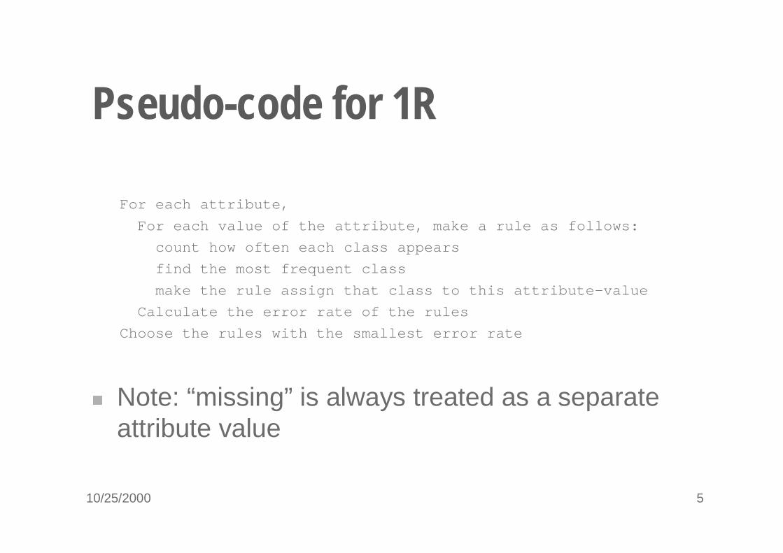
Pseudo-code for 1R

For each attribute,

For each value of the attribute, make a rule as follows:

count how often each class appears

find the most frequent class

make the rule assign that class to this attribute-value

Calculate the error rate of the rules

Choose the rules with the smallest error rate

� Note: “missing” is always treated as a separate attribute value

10/25/2000 6

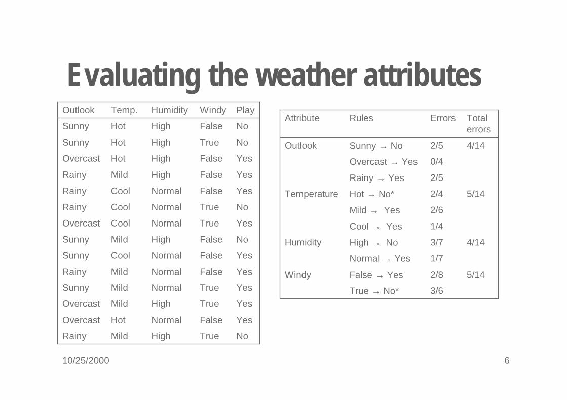
Evaluating the weather attributes

3/6True → No*

5/142/8False → YesWindy

1/7Normal → Yes

4/143/7High → NoHumidity

5/14

4/14

Total errors

1/4Cool → Yes

2/6Mild → Yes

2/4Hot → No*Temperature

2/5Rainy → Yes

0/4Overcast → Yes

2/5Sunny → NoOutlook

ErrorsRulesAttribute

NoTrueHighMildRainy

YesFalseNormalHotOvercast

YesTrueHighMildOvercast

YesTrueNormalMildSunny

YesFalseNormalMildRainy

YesFalseNormalCoolSunny

NoFalseHighMildSunny

YesTrueNormalCoolOvercast

NoTrueNormalCoolRainy

YesFalseNormalCoolRainy

YesFalseHighMildRainy

YesFalseHighHot Overcast

NoTrueHigh Hot Sunny

NoFalseHighHotSunny

PlayWindyHumidityTemp.Outlook

10/25/2000 7

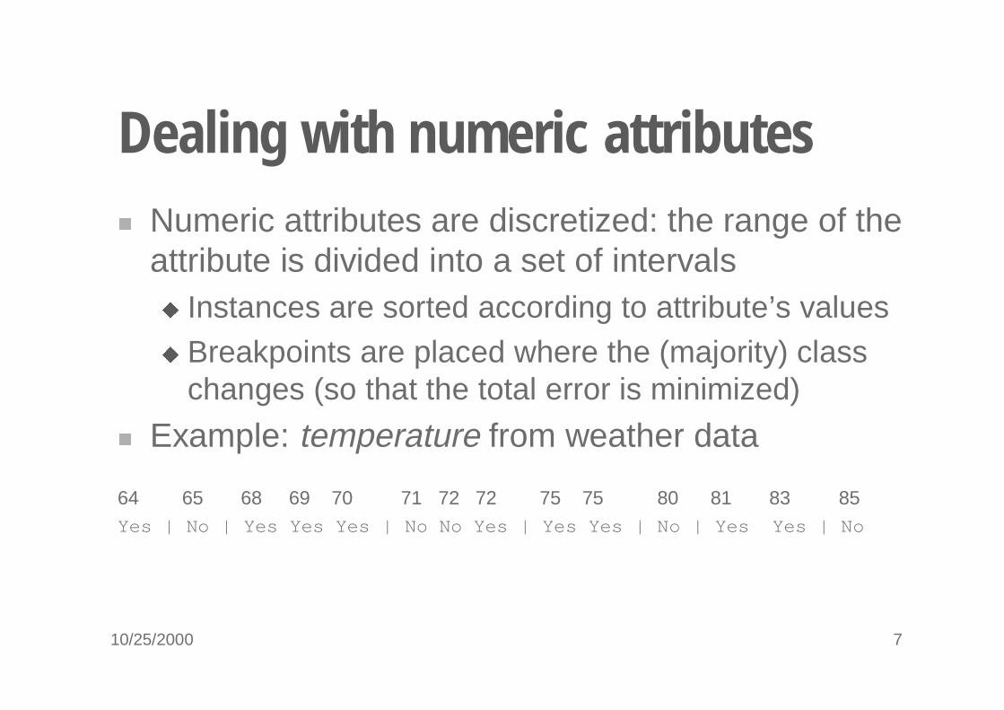
Dealing with numeric attributes� Numeric attributes are discretized: the range of the

attribute is divided into a set of intervals� Instances are sorted according to attribute’s values� Breakpoints are placed where the (majority) class

changes (so that the total error is minimized)

� Example: temperature from weather data

64 65 68 69 70 71 72 72 75 75 80 81 83 85Yes | No | Yes Yes Yes | No No Yes | Yes Yes | No | Yes Yes | No

10/25/2000 8

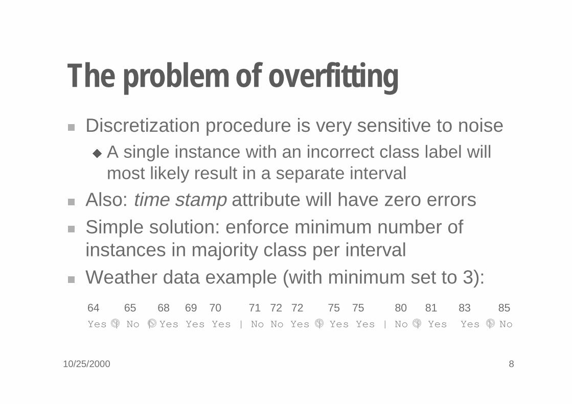
The problem of overfitting� Discretization procedure is very sensitive to noise

� A single instance with an incorrect class label will most likely result in a separate interval

� Also: time stamp attribute will have zero errors� Simple solution: enforce minimum number of

instances in majority class per interval� Weather data example (with minimum set to 3):

64 65 68 69 70 71 72 72 75 75 80 81 83 85Yes | No | Yes Yes Yes | No No Yes | Yes Yes | No | Yes Yes | No

10/25/2000 9

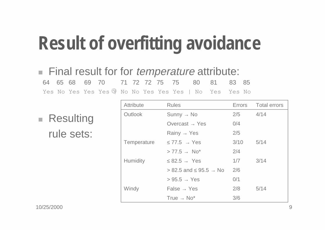
Result of overfitting avoidance� Final result for for temperature attribute:

� Resultingrule sets:

64 65 68 69 70 71 72 72 75 75 80 81 83 85Yes No Yes Yes Yes | No No Yes Yes Yes | No Yes Yes No

0/1> 95.5 → Yes

3/6True → No*

5/142/8False → YesWindy

2/6> 82.5 and ≤ 95.5 → No

3/141/7≤ 82.5 → YesHumidity

5/14

4/14

Total errors

2/4> 77.5 → No*

3/10≤ 77.5 → YesTemperature

2/5Rainy → Yes

0/4Overcast → Yes

2/5Sunny → NoOutlook

ErrorsRulesAttribute

10/25/2000 10

Discussion of 1R� 1R was described in a paper by Holte (1993)

� Contains an experimental evaluation on 16 datasets (using cross-validation so that results were representative of performance on future data)

� Minimum number of instances was set to 6 after some experimentation

� 1R’s simple rules performed not much worse than much more complex decision trees

� Simplicity first pays off!

10/25/2000 11

Statistical modeling� “Opposite” of 1R: use all the attributes� Two assumptions: Attributes are

� equally important� statistically independent (given the class value)

�This means that knowledge about the value of a particular attribute doesn’t tell us anything about the value of another attribute (if the class is known)

� Although based on assumptions that are almost never correct, this scheme works well in practice!

10/25/2000 12

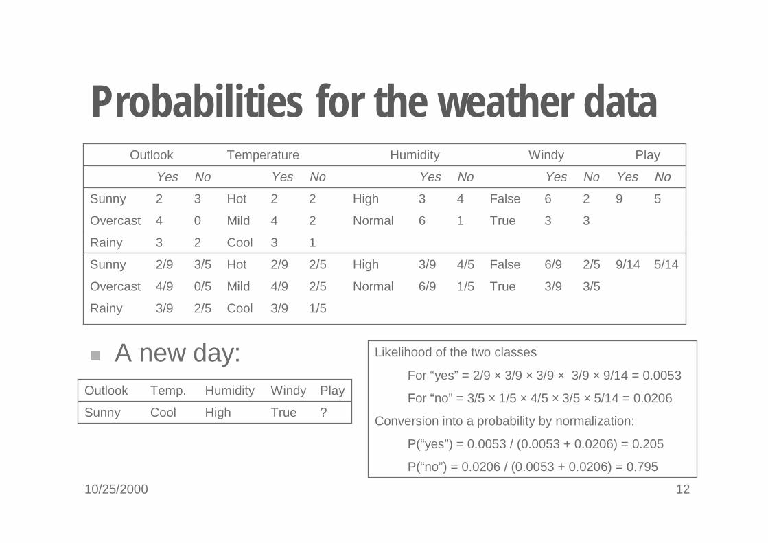
Probabilities for the weather data

5/14

5

No

9/14

9

Yes

Play

3/5

2/5

3

2

No

3/9

6/9

3

6

Yes

True

False

True

False

Windy

1/5

4/5

1

4

NoYesNoYesNoYes

6/9

3/9

6

3

Normal

High

Normal

High

Humidity

1/5

2/5

2/5

1

2

2

3/9

4/9

2/9

3

4

2

Cool2/53/9Rainy

Mild

Hot

Cool

Mild

Hot

Temperature

0/54/9Overcast

3/52/9Sunny

23Rainy

04Overcast

32Sunny

Outlook

?TrueHighCoolSunny


� A new day: Likelihood of the two classes

For “yes” = 2/9 × 3/9 × 3/9 × 3/9 × 9/14 = 0.0053

For “no” = 3/5 × 1/5 × 4/5 × 3/5 × 5/14 = 0.0206

Conversion into a probability by normalization:

P(“yes”) = 0.0053 / (0.0053 + 0.0206) = 0.205

P(“no”) = 0.0206 / (0.0053 + 0.0206) = 0.795

10/25/2000 13

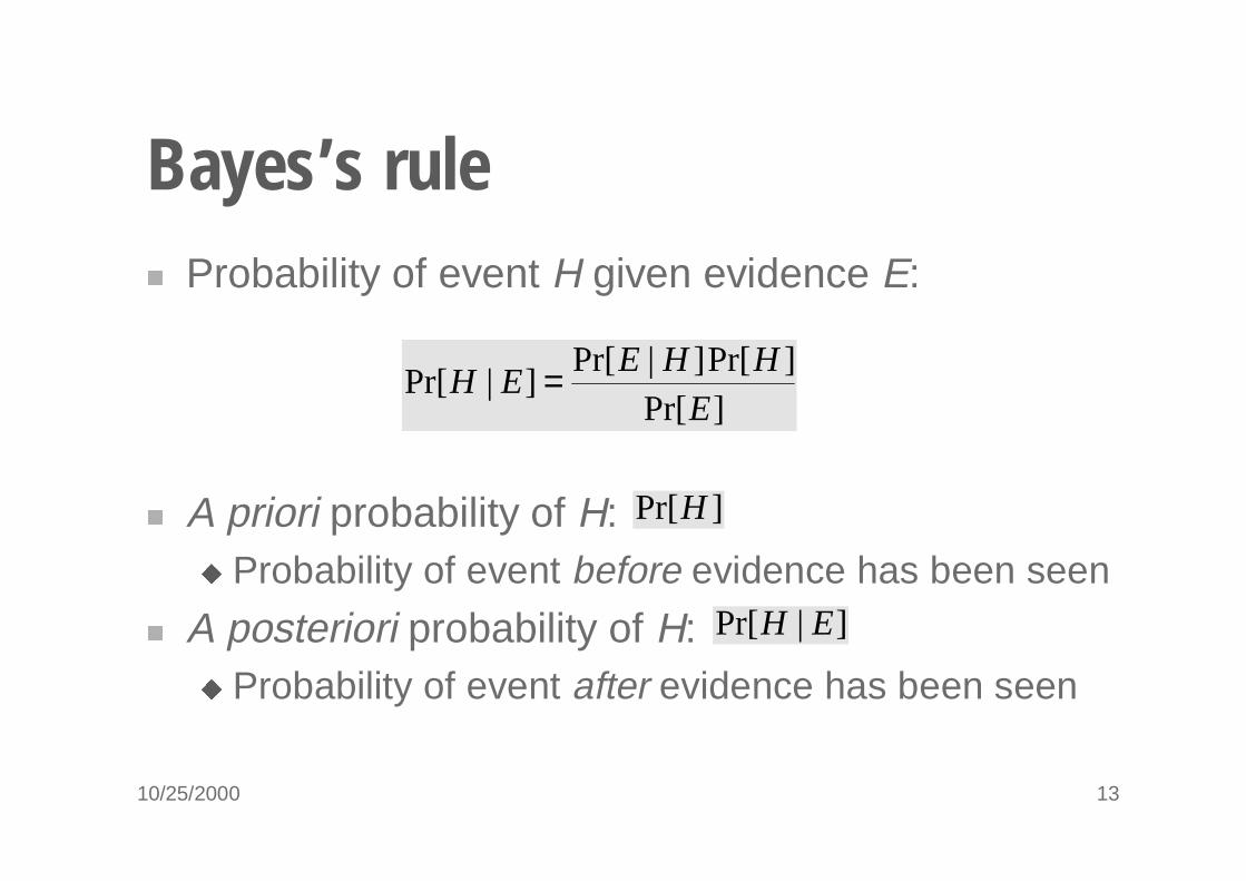
Bayes’s rule� Probability of event H given evidence E:

� A priori probability of H:� Probability of event before evidence has been seen

� A posteriori probability of H:� Probability of event after evidence has been seen

]Pr[]Pr[]|Pr[

]|Pr[E

HHEEH =

]|Pr[ EH

]Pr[H

10/25/2000 14

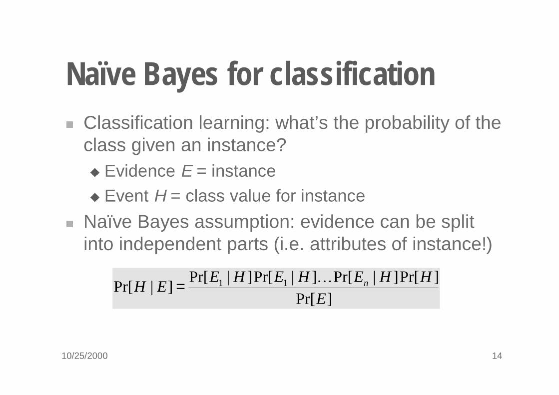
Naïve Bayes for classification� Classification learning: what’s the probability of the

class given an instance? � Evidence E = instance� Event H = class value for instance

� Naïve Bayes assumption: evidence can be split into independent parts (i.e. attributes of instance!)

]Pr[]Pr[]|Pr[]|Pr[]|Pr[

]|Pr[ 11

E

HHEHEHEEH n�=

10/25/2000 15

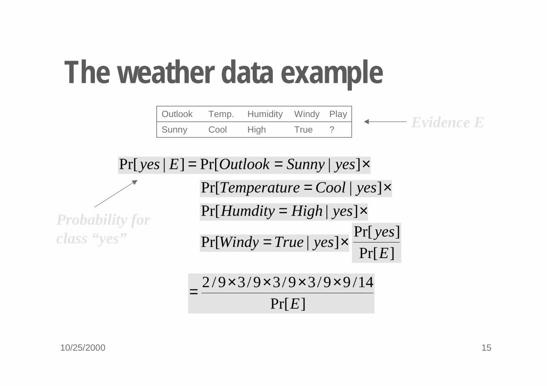
The weather data example

?TrueHighCoolSunny


×== ]|Pr[]|Pr[ yesSunnyOutlookEyes

×= ]|Pr[ yesCooleTemperatur

×= ]|Pr[ yesHighHumdity

×= ]|Pr[ yesTrueWindy]Pr[]Pr[

E

yes

]Pr[14/99/39/39/39/2

E

××××=

Evidence E

Probability forclass “yes”

10/25/2000 16

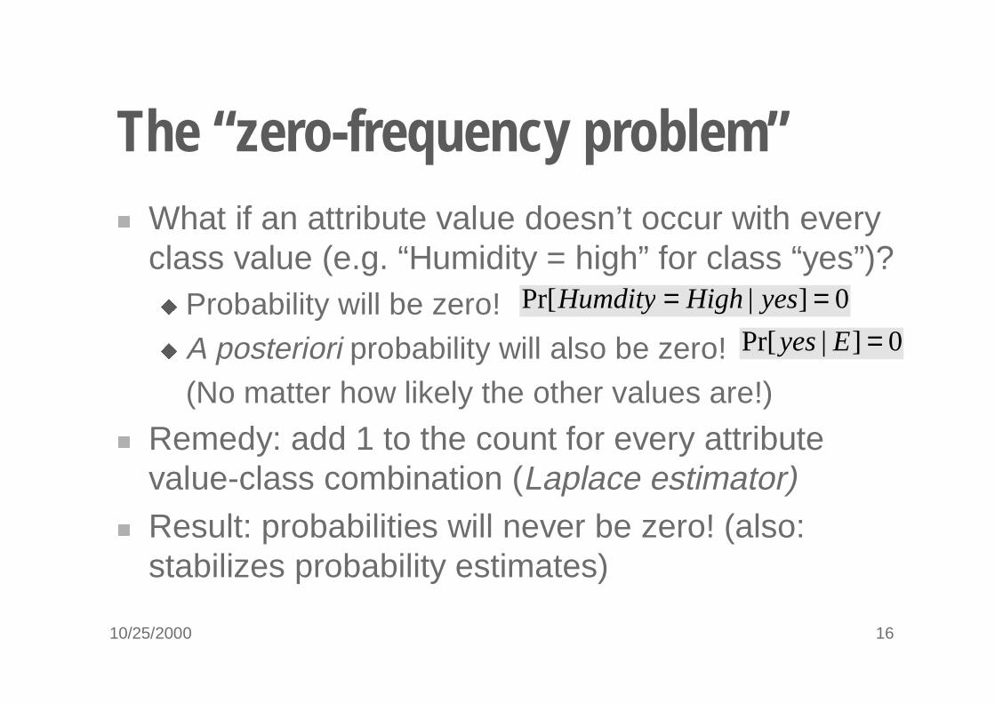
The “zero-frequency problem”� What if an attribute value doesn’t occur with every

class value (e.g. “Humidity = high” for class “yes”)?� Probability will be zero!� A posteriori probability will also be zero!

(No matter how likely the other values are!)

� Remedy: add 1 to the count for every attribute value-class combination (Laplace estimator)

� Result: probabilities will never be zero! (also: stabilizes probability estimates)

0]|Pr[ == yesHighHumdity

0]|Pr[ =Eyes

10/25/2000 17

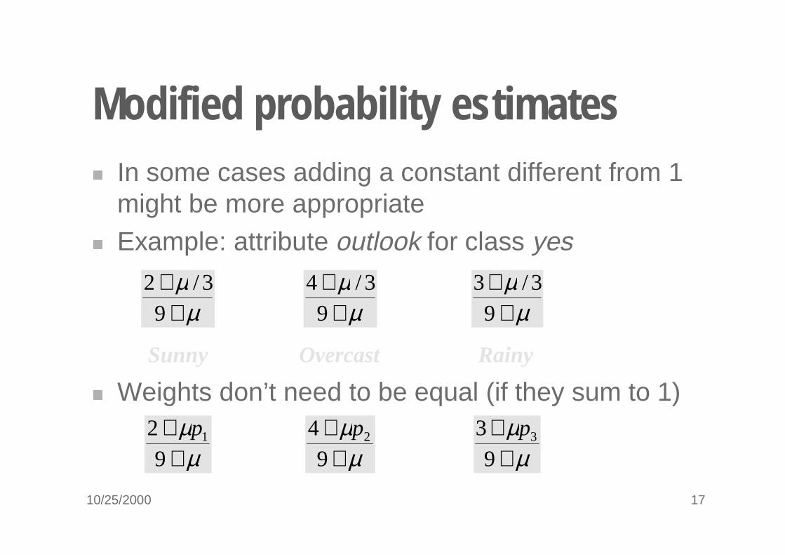
Modified probability estimates� In some cases adding a constant different from 1

might be more appropriate� Example: attribute outlook for class yes

� Weights don’t need to be equal (if they sum to 1)

µµ

++9

3/2µ

µ+

+9

3/4µ

µ+

+9

3/3

Sunny Overcast Rainy

µµ

++

92 1p

µµ

++

94 2p

µµ

++9

3 3p

10/25/2000 18

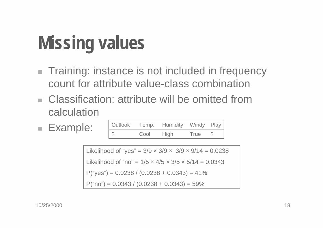
Missing values� Training: instance is not included in frequency

count for attribute value-class combination� Classification: attribute will be omitted from

calculation� Example:

?TrueHighCool?


Likelihood of “yes” = 3/9 × 3/9 × 3/9 × 9/14 = 0.0238

Likelihood of “no” = 1/5 × 4/5 × 3/5 × 5/14 = 0.0343

P(“yes”) = 0.0238 / (0.0238 + 0.0343) = 41%

P(“no”) = 0.0343 / (0.0238 + 0.0343) = 59%

10/25/2000 19

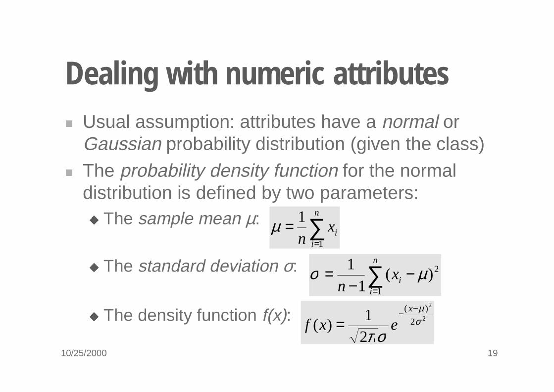
Dealing with numeric attributes� Usual assumption: attributes have a normal or

Gaussian probability distribution (given the class)� The probability density function for the normal

distribution is defined by two parameters:� The sample mean µ:

� The standard deviation σ:

� The density function f(x):

∑=

=n

iix

n 1

1µ

∑=

−−

=n

iix

n 1

2)(1

1 µσ

2

2

2

)(

21

)( σµ

σπ

−−=

x

exf

10/25/2000 20

Statistics for the weather data

� Example density value:

…………

5/14

5

No

9/14

9

Yes

Play

3/5

2/5

3

2

No

3/9

6/9

3

6

Yes

True

False

True

False

Windy

9.7

86.2

70

90

85

NoYesNoYesNoYes

10.2

79.1

80

96

86

std dev

mean

Humidity

7.9

74.6

65

80

85

6.2

73

68

70

83

2/53/9Rainy

std dev

mean

Temperature

0/54/9Overcast

3/52/9Sunny

23Rainy

04Overcast

32Sunny

Outlook

0340.02.62

1)|66(

2

2

2.62

)7366(

=== ∗−−

eyesetemperaturfπ

10/25/2000 21

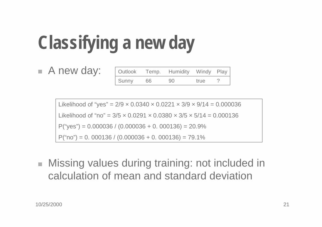
Classifying a new day� A new day:

� Missing values during training: not included in calculation of mean and standard deviation

?true9066Sunny


Likelihood of “yes” = 2/9 × 0.0340 × 0.0221 × 3/9 × 9/14 = 0.000036

Likelihood of “no” = 3/5 × 0.0291 × 0.0380 × 3/5 × 5/14 = 0.000136

P(“yes”) = 0.000036 / (0.000036 + 0. 000136) = 20.9%

P(“no”) = 0. 000136 / (0.000036 + 0. 000136) = 79.1%

10/25/2000 22

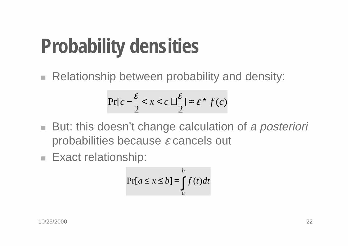
Probability densities� Relationship between probability and density:

� But: this doesn’t change calculation of a posterioriprobabilities because ε cancels out

� Exact relationship:

)(]22

Pr[ cfcxc ∗≈+<<− εεε

∫=≤≤b

a

dttfbxa )(]Pr[

10/25/2000 23

Discussion of Naïve Bayes� Naïve Bayes works surprisingly well (even if

independence assumption is clearly violated)� Why? Because classification doesn’t require

accurate probability estimates as long as maximum probability is assigned to correct class

� However: adding too many redundant attributes will cause problems (e.g. identical attributes)

� Note also: many numeric attributes are not normally distributed (→ kernel density estimators)

10/25/2000 24

Constructing decision trees� Normal procedure: top down in recursive divide-

and-conquer fashion� First: attribute is selected for root node and branch

is created for each possible attribute value� Then: the instances are split into subsets (one for

each branch extending from the node)� Finally: procedure is repeated recursively for each

branch, using only instances that reach the branch

� Process stops if all instances have the same class

10/25/2000 25

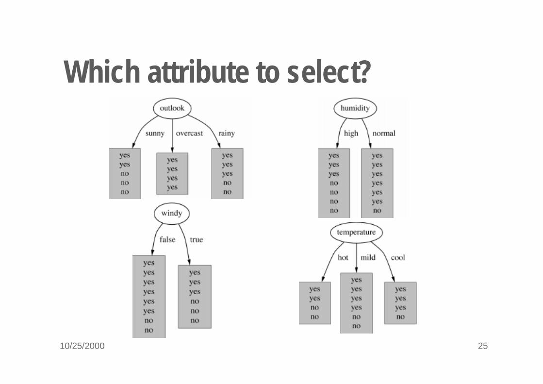
Which attribute to select?

10/25/2000 26

A criterion for attribute selection� Which is the best attribute?

� The one which will result in the smallest tree

� Heuristic: choose the attribute that produces the “purest” nodes

� Popular impurity criterion: information gain� Information gain increases with the average purity

of the subsets that an attribute produces

� Strategy: choose attribute that results in greatest information gain

10/25/2000 27

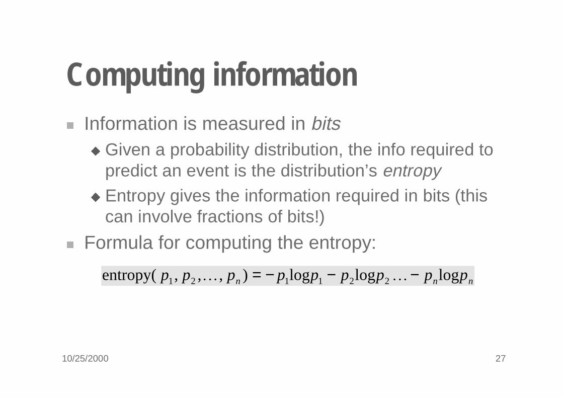
Computing information� Information is measured in bits

� Given a probability distribution, the info required to predict an event is the distribution’s entropy

� Entropy gives the information required in bits (this can involve fractions of bits!)

� Formula for computing the entropy:

nnn ppppppppp logloglog),,,entropy( 221121 −−−= ��

10/25/2000 28

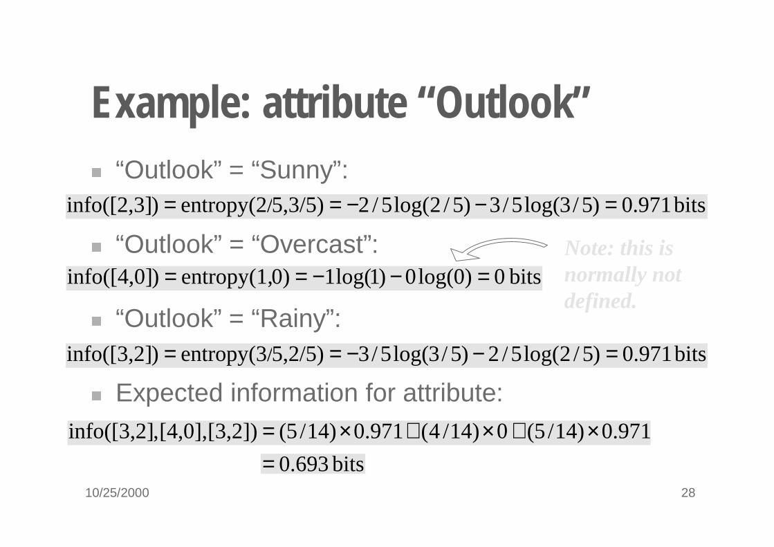
Example: attribute “Outlook” � “Outlook” = “Sunny”:

� “Outlook” = “Overcast”:

� “Outlook” = “Rainy”:

� Expected information for attribute:

bits 971.0)5/3log(5/3)5/2log(5/25,3/5)entropy(2/)info([2,3] =−−==

bits 0)0log(0)1log(10)entropy(1,)info([4,0] =−−==

bits 971.0)5/2log(5/2)5/3log(5/35,2/5)entropy(3/)info([3,2] =−−==

Note: this isnormally notdefined.

971.0)14/5(0)14/4(971.0)14/5([3,2])[4,0],,info([3,2] ×+×+×=bits 693.0=

10/25/2000 29

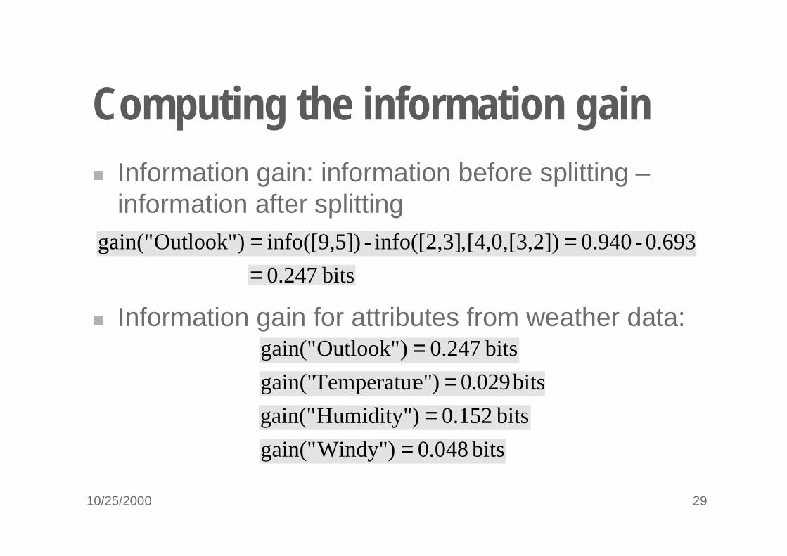
Computing the information gain� Information gain: information before splitting –

information after splitting

� Information gain for attributes from weather data:

0.693-0.940[3,2])[4,0,,info([2,3]-)info([9,5])Outlook"gain(" ==bits 247.0=

bits 247.0)Outlook"gain(" =bits 029.0)e"Temperaturgain(" =

bits 152.0)Humidity"gain(" =bits 048.0)Windy"gain(" =

10/25/2000 30

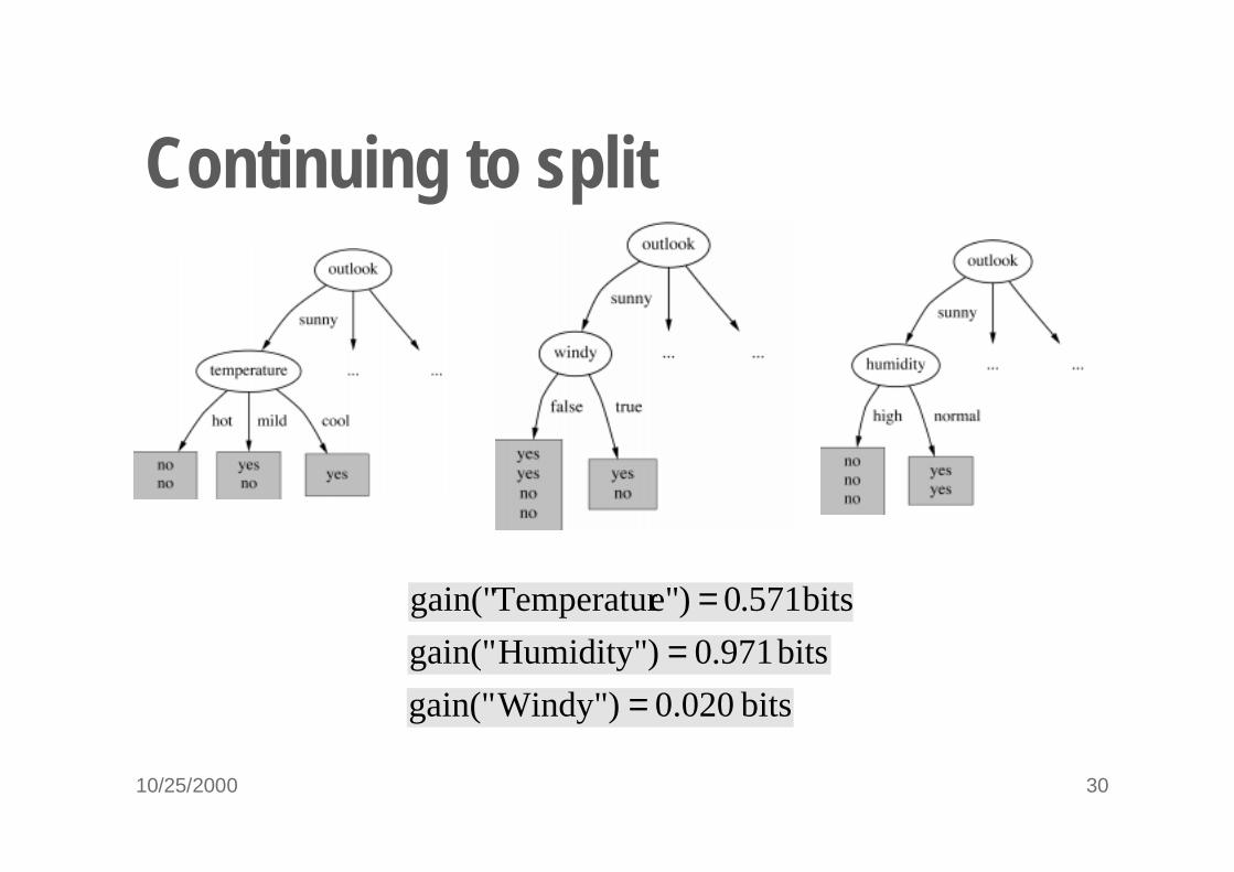
Continuing to split

bits 571.0)e"Temperaturgain(" =bits 971.0)Humidity"gain(" =

bits 020.0)Windy"gain(" =

10/25/2000 31

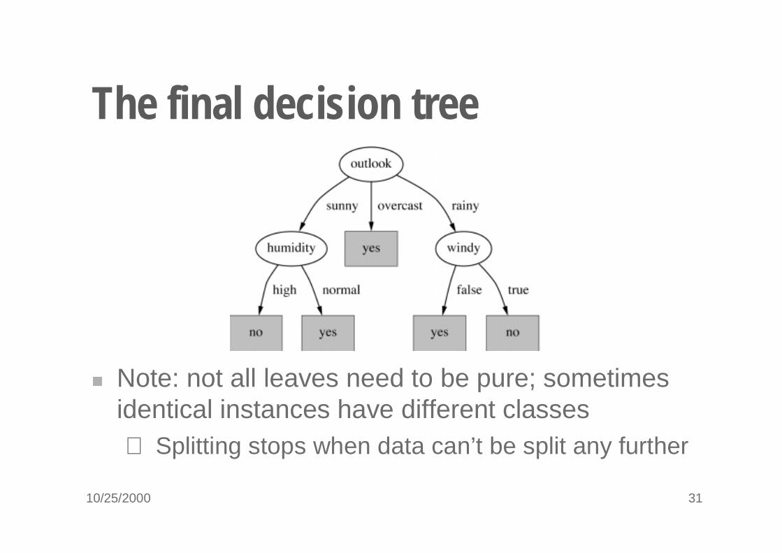
The final decision tree

� Note: not all leaves need to be pure; sometimes identical instances have different classes⇒ Splitting stops when data can’t be split any further

10/25/2000 32

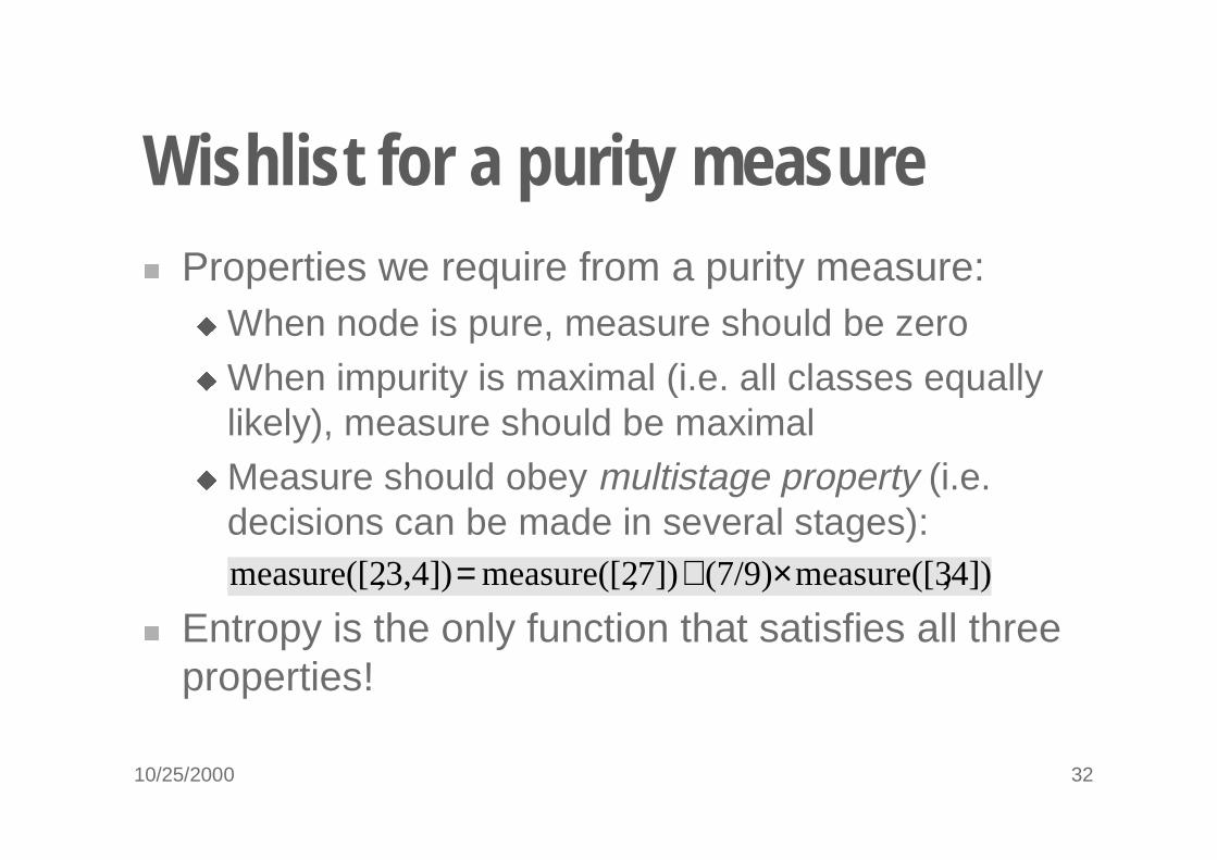
Wishlist for a purity measure� Properties we require from a purity measure:

� When node is pure, measure should be zero

� When impurity is maximal (i.e. all classes equally likely), measure should be maximal

� Measure should obey multistage property (i.e. decisions can be made in several stages):

� Entropy is the only function that satisfies all three properties!

,4])measure([3(7/9),7])measure([2,3,4])measure([2 ×+=

10/25/2000 33

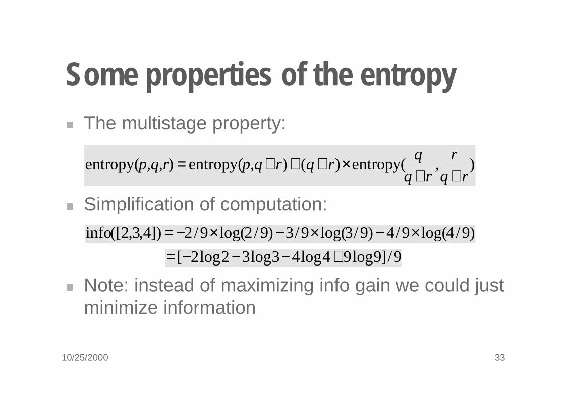
Some properties of the entropy� The multistage property:

� Simplification of computation:

� Note: instead of maximizing info gain we could just minimize information

)entropy()()entropy()entropy(rq

r,

rq

qrqrp,qp,q,r

++×+++=

)9/4log(9/4)9/3log(9/3)9/2log(9/2])4,3,2([info ×−×−×−=9/]9log94log43log32log2[ +−−−=

10/25/2000 34

Highly-branching attributes� Problematic: attributes with a large number of

values (extreme case: ID code)� Subsets are more likely to be pure if there is a

large number of values⇒ Information gain is biased towards choosing

attributes with a large number of values⇒ This may result in overfitting (selection of an

attribute that is non-optimal for prediction)

� Another problem: fragmentation

10/25/2000 35

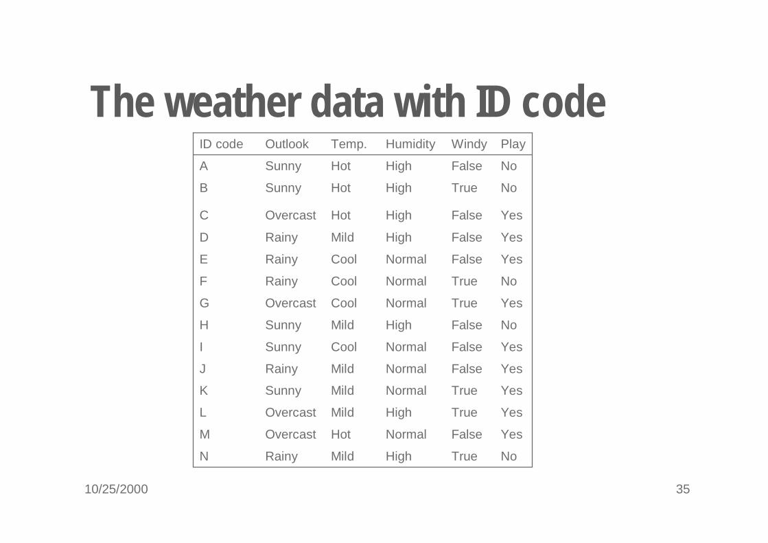
The weather data with ID code

N

M

L

K

J

I

H

G

F

E

D

C

B

A

ID code

NoTrueHighMildRainy

YesFalseNormalHotOvercast

YesTrueHighMildOvercast

YesTrueNormalMildSunny

YesFalseNormalMildRainy

YesFalseNormalCoolSunny

NoFalseHighMildSunny

YesTrueNormalCoolOvercast

NoTrueNormalCoolRainy

YesFalseNormalCoolRainy

YesFalseHighMildRainy

YesFalseHighHot Overcast

NoTrueHigh Hot Sunny

NoFalseHighHotSunny


10/25/2000 36

Tree stump for ID code attribute

� Entropy of split:

⇒ Information gain is maximal for ID code (namely 0.940 bits)

bits 0)info([0,1])info([0,1])info([0,1])code" ID"(info =+++= �

10/25/2000 37

The gain ratio� Gain ratio: a modification of the information gain

that reduces its bias� Gain ratio takes number and size of branches into

account when choosing an attribute� It corrects the information gain by taking the

intrinsic information of a split into account

� Intrinsic information: entropy of distribution of instances into branches (i.e. how much info do we need to tell which branch an instance belongs to)

10/25/2000 38

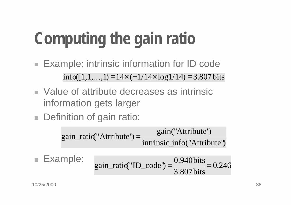
Computing the gain ratio� Example: intrinsic information for ID code

� Value of attribute decreases as intrinsic information gets larger

� Definition of gain ratio:

� Example:

bits 807.3)14/1log14/1(14),1[1,1,(info =×−×=�

)Attribute"info("intrinsic_)Attribute"gain("

)Attribute"("gain_ratio =

246.0bits 3.807bits 0.940

)ID_code"("gain_ratio ==

10/25/2000 39

Gain ratios for weather data

0.021Gain ratio: 0.029/1.3620.156Gain ratio: 0.247/1.577

1.362Split info: info([4,6,4])1.577 Split info: info([5,4,5])

0.029Gain: 0.940-0.911 0.247 Gain: 0.940-0.693

0.911Info:0.693Info:

TemperatureOutlook

0.049Gain ratio: 0.048/0.9850.152Gain ratio: 0.152/1

0.985Split info: info([8,6])1.000 Split info: info([7,7])

0.048Gain: 0.940-0.892 0.152Gain: 0.940-0.788

0.892Info:0.788Info:

WindyHumidity

10/25/2000 40

More on the gain ratio� “Outlook” still comes out top� However: “ID code” has greater gain ratio

� Standard fix: ad hoc test to prevent splitting on that type of attribute

� Problem with gain ratio: it may overcompensate� May choose an attribute just because its intrinsic

information is very low� Standard fix: only consider attributes with greater

than average information gain

10/25/2000 41

Discussion� Algorithm for top-down induction of decision trees

(“ID3”) was developed by Ross Quinlan� Gain ratio just one modification of this basic

algorithm� Led to development of C4.5, which can deal with

numeric attributes, missing values, and noisy data

� Similar approach: CART� There are many other attribute selection criteria!

(But almost no difference in accuracy of result.)

10/25/2000 42

Covering algorithms� Decision tree can be converted into a rule set

� Straightforward conversion: rule set overly complex

� More effective conversions are not trivial

� Strategy for generating a rule set directly: for each class in turn find rule set that covers all instances in it (excluding instances not in the class)

� This approach is called a covering approach because at each stage a rule is identified that covers some of the instances

10/25/2000 43

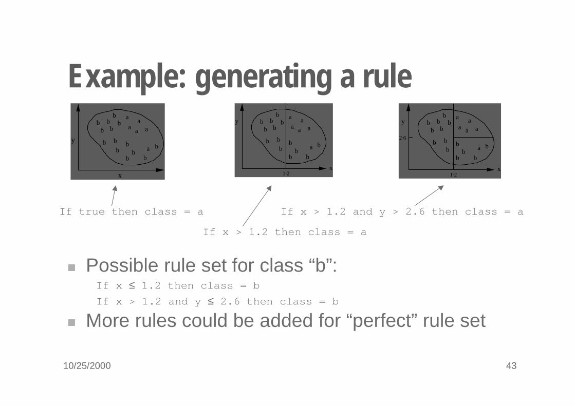
Example: generating a rule

y

x

a

b b

b

b

b

bb

b

b b bb

bb

aa

aa

ay

a

b b

b

b

b

bb

b

b b bb

bb

a a

aa

a

x1·2

y

a

b b

b

b

b

bb

b

b b bb

bb

a a

aa

a

x1·2

2·6

If x > 1.2 then class = a

If x > 1.2 and y > 2.6 then class = aIf true then class = a

� Possible rule set for class “b”:

� More rules could be added for “perfect” rule set

If x ≤ 1.2 then class = b

If x > 1.2 and y ≤ 2.6 then class = b

10/25/2000 44

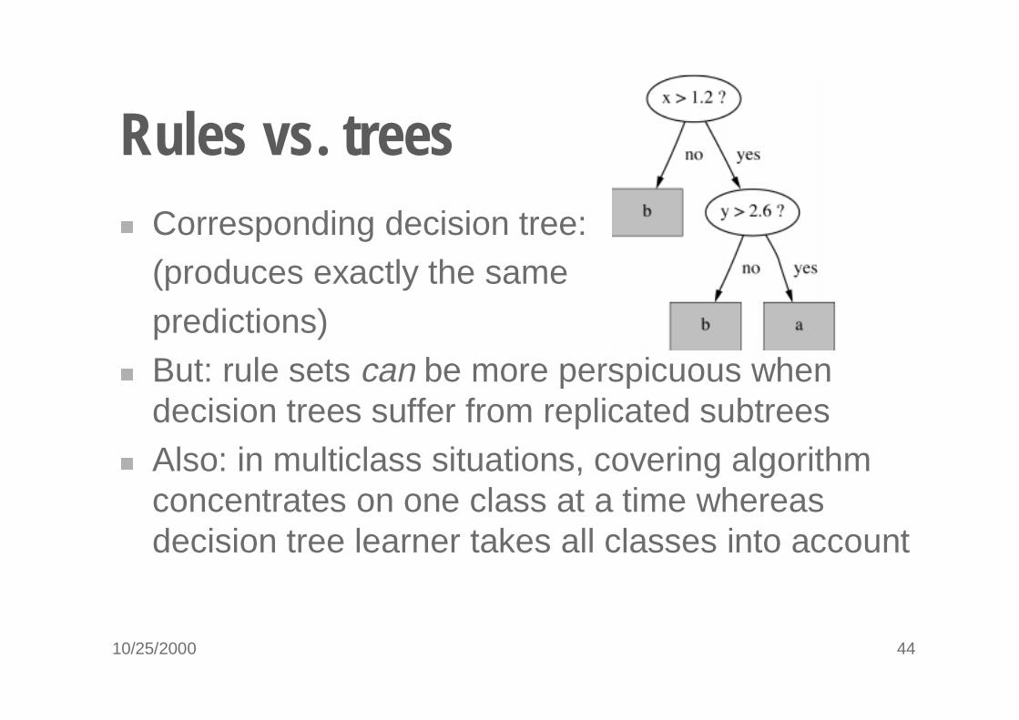
Rules vs. trees� Corresponding decision tree:

(produces exactly the samepredictions)

� But: rule sets can be more perspicuous when decision trees suffer from replicated subtrees

� Also: in multiclass situations, covering algorithm concentrates on one class at a time whereas decision tree learner takes all classes into account

10/25/2000 45

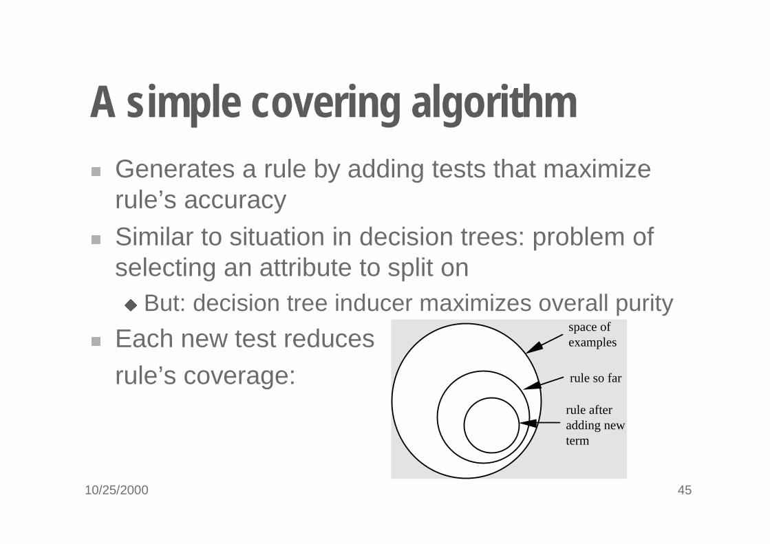
A simple covering algorithm� Generates a rule by adding tests that maximize

rule’s accuracy� Similar to situation in decision trees: problem of

selecting an attribute to split on� But: decision tree inducer maximizes overall purity

� Each new test reducesrule’s coverage:

space of examples

rule so far

rule after adding new term

10/25/2000 46

Selecting a test� Goal: maximizing accuracy

� t: total number of instances covered by rule

� p: positive examples of the class covered by rule� t-p: number of errors made by rule⇒ Select test that maximizes the ratio p/t

� We are finished when p/t = 1 or the set of instances can’t be split any further

10/25/2000 47

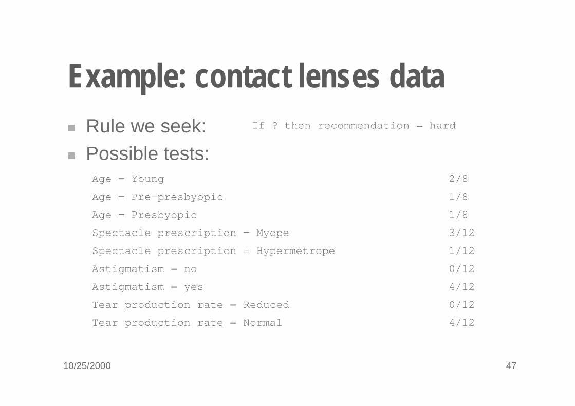
Example: contact lenses data� Rule we seek:� Possible tests:

4/12Tear production rate = Normal

0/12Tear production rate = Reduced

4/12Astigmatism = yes

0/12Astigmatism = no

1/12Spectacle prescription = Hypermetrope

3/12Spectacle prescription = Myope

1/8Age = Presbyopic

1/8Age = Pre-presbyopic

2/8Age = Young

If ? then recommendation = hard

10/25/2000 48

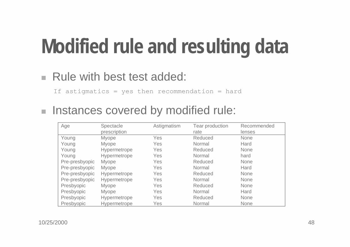
Modified rule and resulting data� Rule with best test added:

� Instances covered by modified rule:

If astigmatics = yes then recommendation = hard

NoneReducedYesHypermetropePre-presbyopic NoneNormalYesHypermetropePre-presbyopicNoneReducedYesMyopePresbyopicHardNormalYesMyopePresbyopicNoneReducedYesHypermetropePresbyopicNoneNormalYesHypermetropePresbyopic

HardNormalYesMyopePre-presbyopicNoneReducedYesMyopePre-presbyopichardNormalYesHypermetropeYoungNoneReducedYesHypermetropeYoungHardNormalYesMyopeYoungNoneReducedYesMyopeYoung

Recommended lenses

Tear production rate

AstigmatismSpectacle prescription

Age

10/25/2000 49

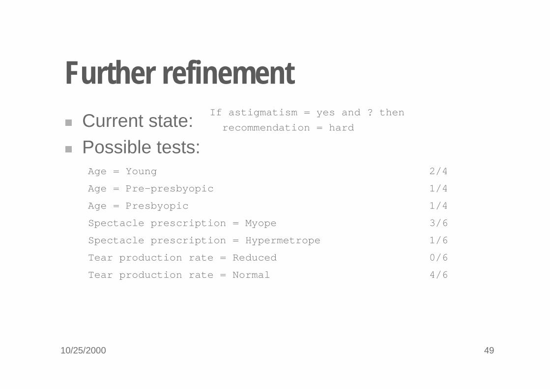
Further refinement� Current state:� Possible tests:

4/6Tear production rate = Normal

0/6Tear production rate = Reduced



1/4Age = Presbyopic


2/4Age = Young

If astigmatism = yes and ? then

recommendation = hard

10/25/2000 50

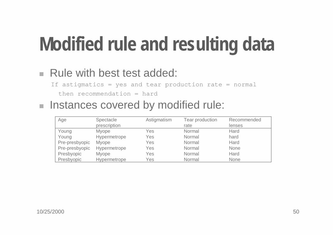
Modified rule and resulting data� Rule with best test added:

� Instances covered by modified rule:

If astigmatics = yes and tear production rate = normal

then recommendation = hard

NoneNormalYesHypermetropePre-presbyopicHardNormalYesMyopePresbyopicNoneNormalYesHypermetropePresbyopic

HardNormalYesMyopePre-presbyopichardNormalYesHypermetropeYoungHardNormalYesMyopeYoung

Recommended lenses

Tear production rate

AstigmatismSpectacle prescription

Age

10/25/2000 51

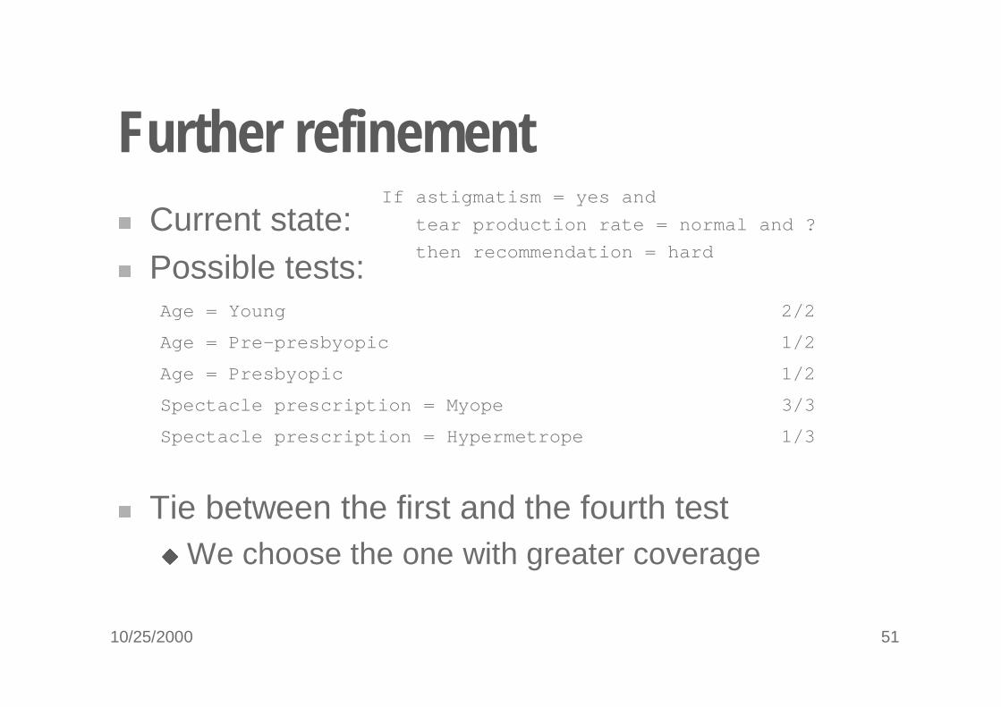
Further refinement� Current state:� Possible tests:

� Tie between the first and the fourth test� We choose the one with greater coverage



1/2Age = Presbyopic


2/2Age = Young

If astigmatism = yes and

tear production rate = normal and ?


10/25/2000 52

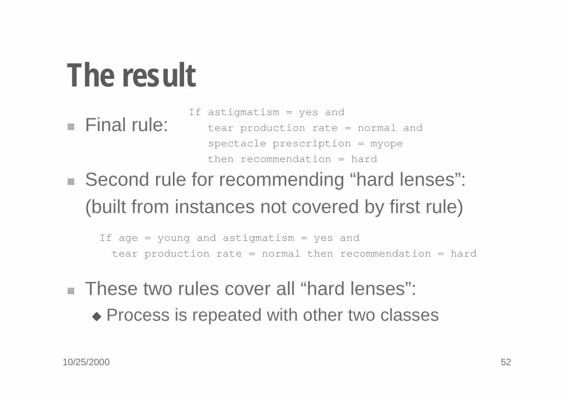
The result� Final rule:

� Second rule for recommending “hard lenses”:(built from instances not covered by first rule)

� These two rules cover all “hard lenses”:� Process is repeated with other two classes

If astigmatism = yes and

tear production rate = normal and

spectacle prescription = myope


If age = young and astigmatism = yes and

tear production rate = normal then recommendation = hard

10/25/2000 53

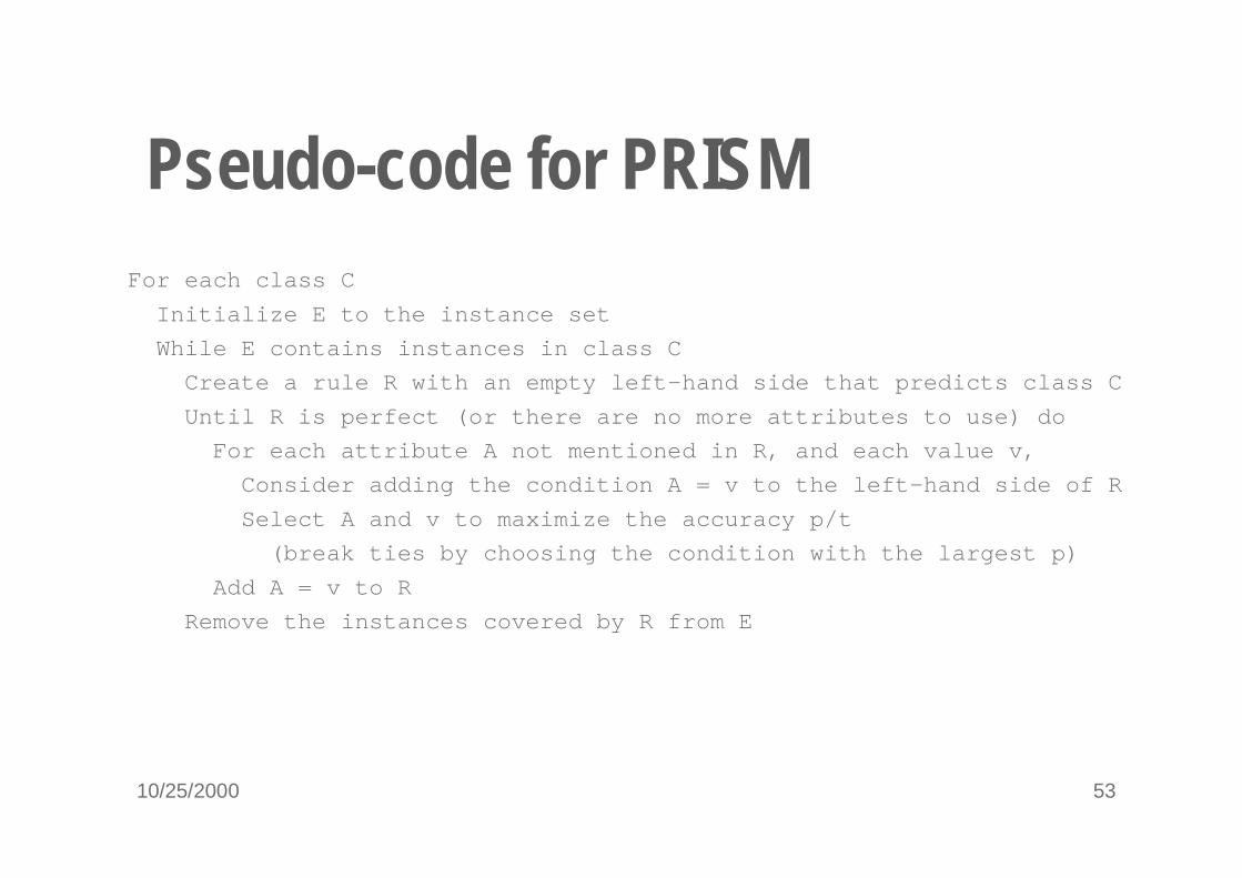
Pseudo-code for PRISMFor each class C

Initialize E to the instance set

While E contains instances in class C

Create a rule R with an empty left-hand side that predicts class C

Until R is perfect (or there are no more attributes to use) do

For each attribute A not mentioned in R, and each value v,

Consider adding the condition A = v to the left-hand side of R

Select A and v to maximize the accuracy p/t

(break ties by choosing the condition with the largest p)

Add A = v to R

Remove the instances covered by R from E

10/25/2000 54

Rules vs. decision lists� PRISM with outer loop removed generates a

decision list for one class� Subsequent rules are designed for rules that are

not covered by previous rules� But: order doesn’t matter because all rules predict

the same class

� Outer loop considers all classes separately� No order dependence implied

� Problems: overlapping rules, default rule required

10/25/2000 55

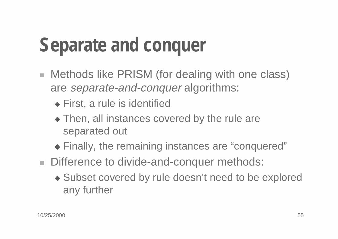
Separate and conquer� Methods like PRISM (for dealing with one class)

are separate-and-conquer algorithms:� First, a rule is identified� Then, all instances covered by the rule are

separated out� Finally, the remaining instances are “conquered”

� Difference to divide-and-conquer methods:� Subset covered by rule doesn’t need to be explored

any further

10/25/2000 56

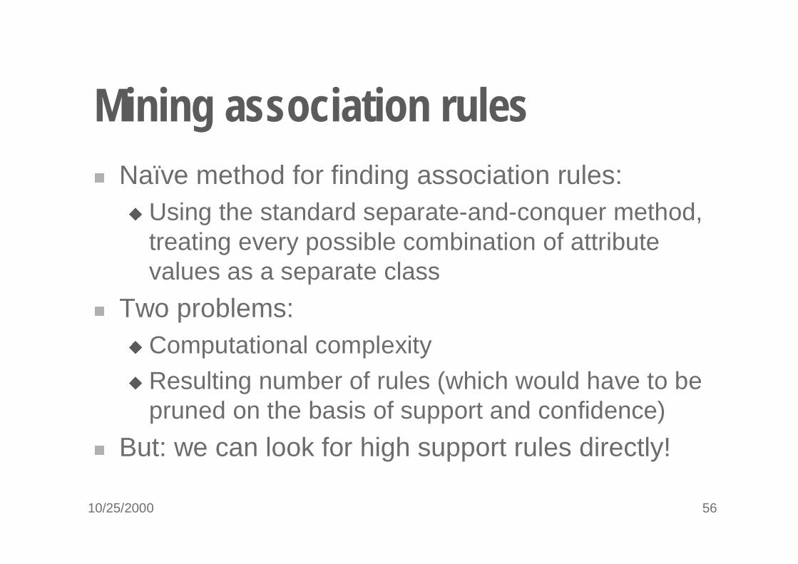
Mining association rules� Naïve method for finding association rules:

� Using the standard separate-and-conquer method, treating every possible combination of attribute values as a separate class

� Two problems:� Computational complexity

� Resulting number of rules (which would have to be pruned on the basis of support and confidence)

� But: we can look for high support rules directly!

10/25/2000 57

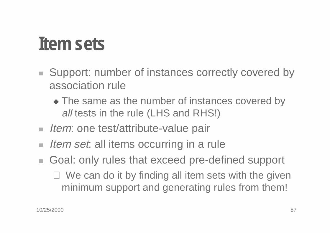
Item sets� Support: number of instances correctly covered by

association rule� The same as the number of instances covered by

all tests in the rule (LHS and RHS!)

� Item: one test/attribute-value pair� Item set: all items occurring in a rule� Goal: only rules that exceed pre-defined support

⇒ We can do it by finding all item sets with the given minimum support and generating rules from them!

10/25/2000 58

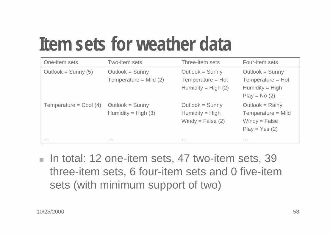
Item sets for weather data

…………

Outlook = Rainy

Temperature = Mild

Windy = False

Play = Yes (2)

Outlook = Sunny

Humidity = High

Windy = False (2)

Outlook = Sunny

Humidity = High (3)

Temperature = Cool (4)

Outlook = Sunny

Temperature = Hot

Humidity = High

Play = No (2)

Outlook = Sunny

Temperature = Hot

Humidity = High (2)

Outlook = Sunny

Temperature = Mild (2)

Outlook = Sunny (5)

Four-item setsThree-item setsTwo-item setsOne-item sets

� In total: 12 one-item sets, 47 two-item sets, 39 three-item sets, 6 four-item sets and 0 five-item sets (with minimum support of two)

10/25/2000 59

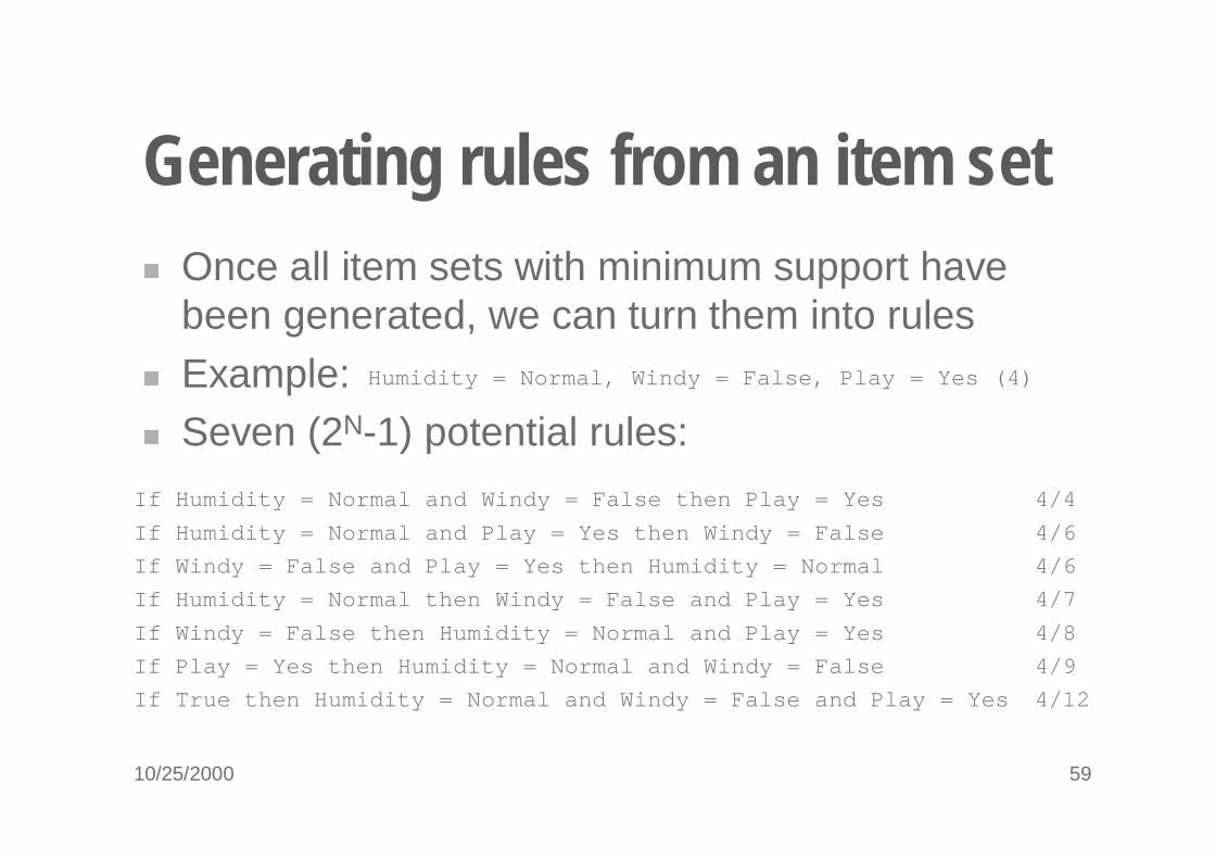
Generating rules from an item set� Once all item sets with minimum support have

been generated, we can turn them into rules� Example:� Seven (2N-1) potential rules:

Humidity = Normal, Windy = False, Play = Yes (4)

4/4

4/6

4/6

4/7

4/8

4/9

4/12

If Humidity = Normal and Windy = False then Play = Yes

If Humidity = Normal and Play = Yes then Windy = False

If Windy = False and Play = Yes then Humidity = Normal

If Humidity = Normal then Windy = False and Play = Yes

If Windy = False then Humidity = Normal and Play = Yes

If Play = Yes then Humidity = Normal and Windy = False

If True then Humidity = Normal and Windy = False and Play = Yes

10/25/2000 60

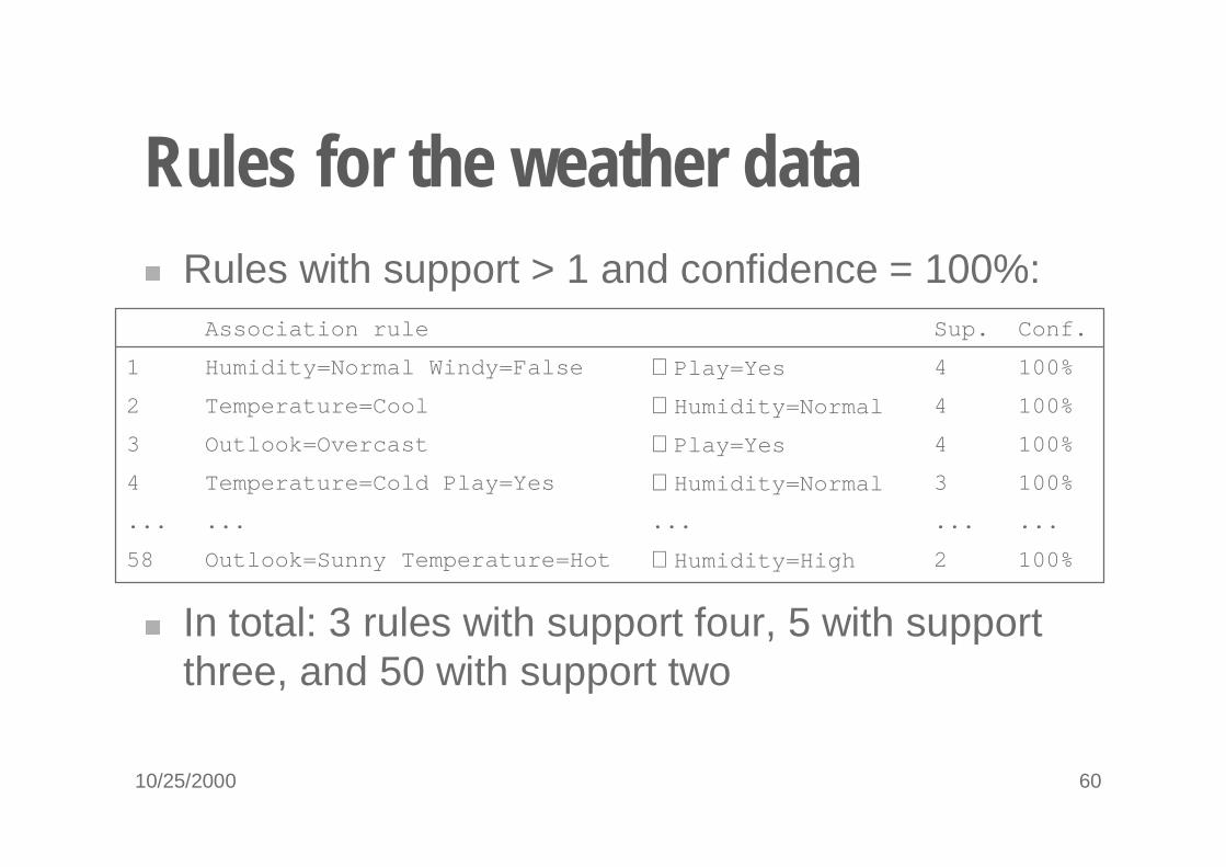
Rules for the weather data� Rules with support > 1 and confidence = 100%:

� In total: 3 rules with support four, 5 with support three, and 50 with support two

100%2⇒Humidity=HighOutlook=Sunny Temperature=Hot58

...............

100%3⇒Humidity=NormalTemperature=Cold Play=Yes4

100%4⇒Play=YesOutlook=Overcast3

100%4⇒Humidity=NormalTemperature=Cool2

100%4⇒Play=YesHumidity=Normal Windy=False1

Association rule Conf.Sup.

10/25/2000 61

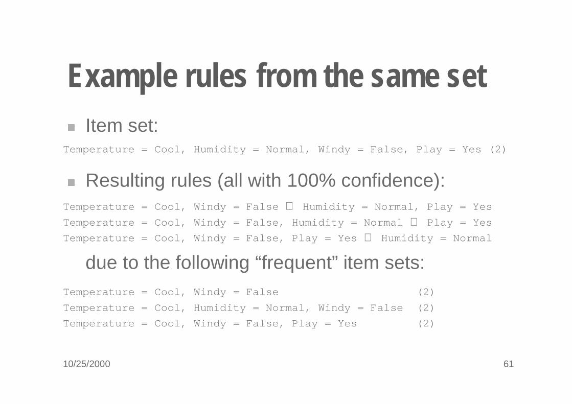
Example rules from the same set� Item set:

� Resulting rules (all with 100% confidence):

due to the following “frequent” item sets:

Temperature = Cool, Humidity = Normal, Windy = False, Play = Yes (2)

Temperature = Cool, Windy = False ⇒ Humidity = Normal, Play = Yes

Temperature = Cool, Windy = False, Humidity = Normal ⇒ Play = Yes

Temperature = Cool, Windy = False, Play = Yes ⇒ Humidity = Normal

Temperature = Cool, Windy = False (2)

Temperature = Cool, Humidity = Normal, Windy = False (2)

Temperature = Cool, Windy = False, Play = Yes (2)

10/25/2000 62

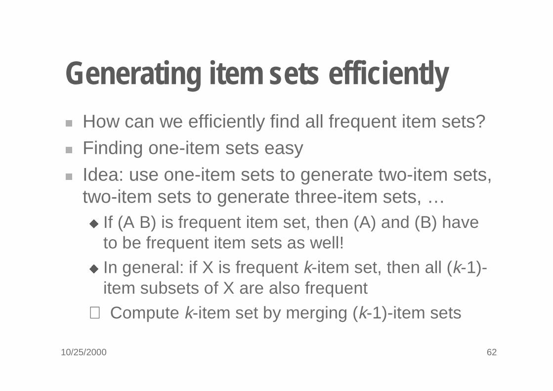
Generating item sets efficiently� How can we efficiently find all frequent item sets?� Finding one-item sets easy� Idea: use one-item sets to generate two-item sets,

two-item sets to generate three-item sets, …� If (A B) is frequent item set, then (A) and (B) have

to be frequent item sets as well!� In general: if X is frequent k-item set, then all (k-1)-

item subsets of X are also frequent

⇒ Compute k-item set by merging (k-1)-item sets

10/25/2000 63

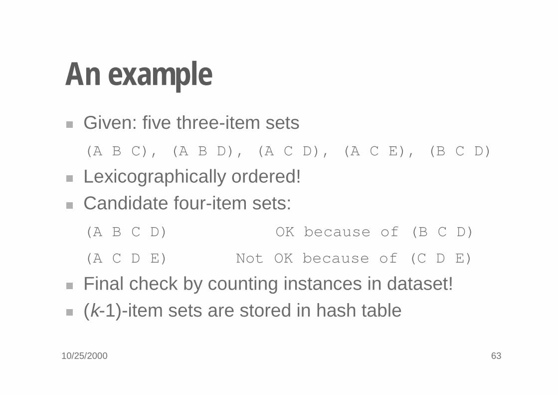
An example� Given: five three-item sets(A B C), (A B D), (A C D), (A C E), (B C D)

� Lexicographically ordered!� Candidate four-item sets:(A B C D) OK because of (B C D)

(A C D E) Not OK because of (C D E)

� Final check by counting instances in dataset!� (k-1)-item sets are stored in hash table

10/25/2000 64

Generating rules efficiently� We are looking for all high-confidence rules

� Support of antecedent obtained from hash table

� But: brute-force method is (2N-1)

� Better way: building (c + 1)-consequent rules from c-consequent ones� Observation: (c + 1)-consequent rule can only hold

if all corresponding c-consequent rules also hold

� Resulting algorithm similar to procedure for large item sets

10/25/2000 65

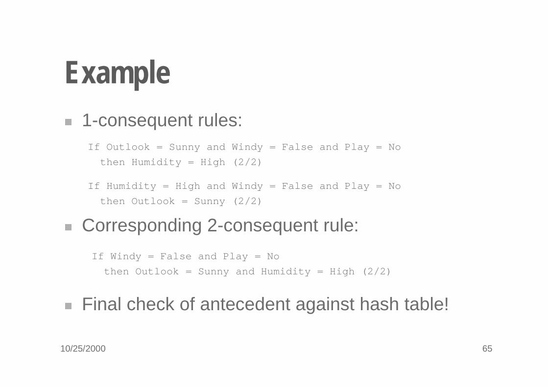
Example� 1-consequent rules:

� Corresponding 2-consequent rule:

� Final check of antecedent against hash table!

If Windy = False and Play = No

then Outlook = Sunny and Humidity = High (2/2)

If Outlook = Sunny and Windy = False and Play = No

then Humidity = High (2/2)

If Humidity = High and Windy = False and Play = No

then Outlook = Sunny (2/2)

10/25/2000 66

Discussion of association rules� Above method makes one pass through the data

for each different size item set� Other possibility: generate (k+2)-item sets just after

(k+1)-item sets have been generated� Result: more (k+2)-item sets than necessary will be

considered but less passes through the data� Makes sense if data too large for main memory

� Practical issue: generating a certain number of rules (e.g. by incrementally reducing min. support)

10/25/2000 67

Other issues� ARFF format very inefficient for typical market

basket data� Attributes represent items in a basket and most

items are usually missing

� Instances are also called transactions� Confidence is not necessarily the best measure

� Example: milk occurs in almost every supermarket transaction

� Other measures have been devised (e.g. lift)

10/25/2000 68

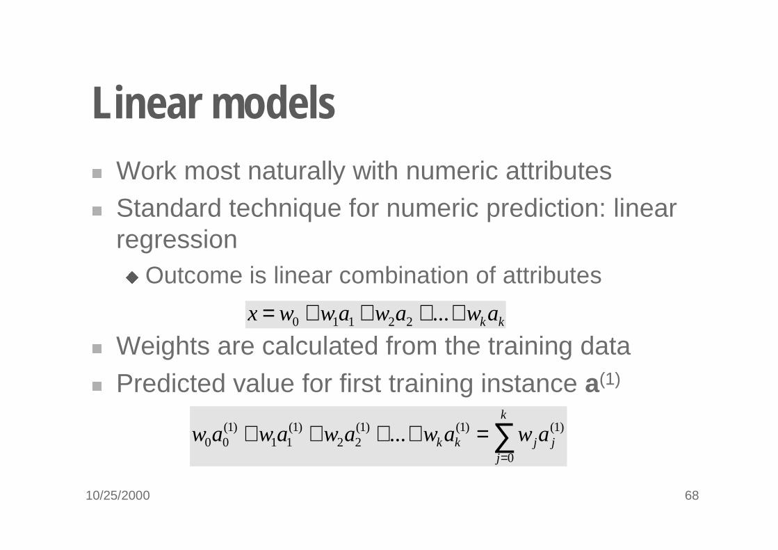
Linear models� Work most naturally with numeric attributes� Standard technique for numeric prediction: linear

regression� Outcome is linear combination of attributes

� Weights are calculated from the training data� Predicted value for first training instance a(1)

kkawawawwx ++++= ...22110

∑=

=++++k

jjjkk awawawawaw

0

)1()1()1(22

)1(11

)1(00 ...

10/25/2000 69

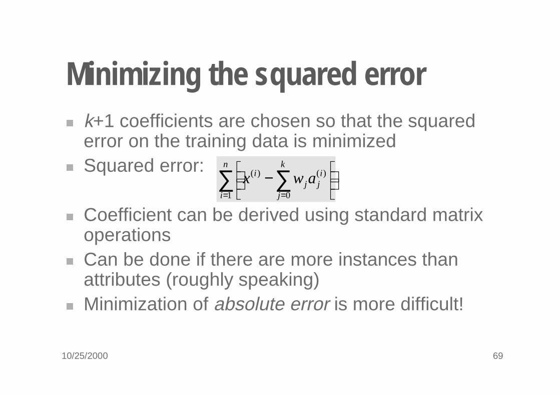
Minimizing the squared error� k+1 coefficients are chosen so that the squared

error on the training data is minimized� Squared error:

� Coefficient can be derived using standard matrix operations

� Can be done if there are more instances than attributes (roughly speaking)

� Minimization of absolute error is more difficult!

∑ ∑= =

−

n

i

k

j

ijj

i awx1 0

)()(

10/25/2000 70

Classification� Any regression technique can be used for

classification� Training: perform a regression for each class,

setting the output to 1 for training instances that belong to class, and 0 for those that don’t

� Prediction: predict class corresponding to model with largest output value (membership value)

� For linear regression this is known as multi-response linear regression

10/25/2000 71

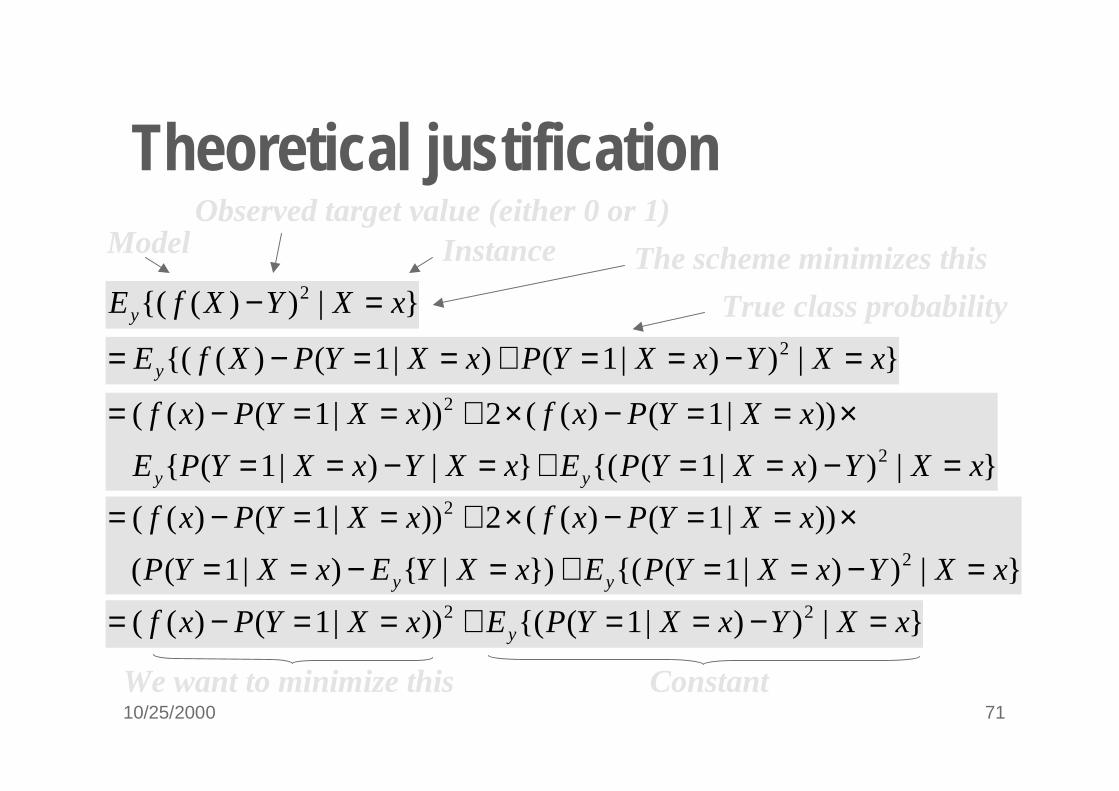
Theoretical justification

}|))({( 2 xXYXfEy =−

}|))|1()|1()({( 2 xXYxXYPxXYPXfEy =−==+==−=

}|))|1({(})|{)|1((

))|1()((2))|1()((2

2

xXYxXYPExXYExXYP

xXYPxfxXYPxf

yy =−==+=−==

×==−×+==−=}|))|1({(}|)|1({

))|1()((2))|1()((2

2

xXYxXYPExXYxXYPE

xXYPxfxXYPxf

yy =−==+=−==

×==−×+==−=

}|))|1({())|1()(( 22 xXYxXYPExXYPxf y =−==+==−=

Model InstanceObserved target value (either 0 or 1)

True class probability

ConstantWe want to minimize this

The scheme minimizes this

10/25/2000 72

Pairwise regression� Another way of using regression for classification:

� A regression function for every pair of classes, using only instances from these two classes

� An output of +1 is assigned to one member of the pair, an output of –1 to the other

� Prediction is done by voting� Class that receives most votes is predicted� Alternative: “don’t know” if there is no agreement

� More likely to be accurate but more expensive

10/25/2000 73

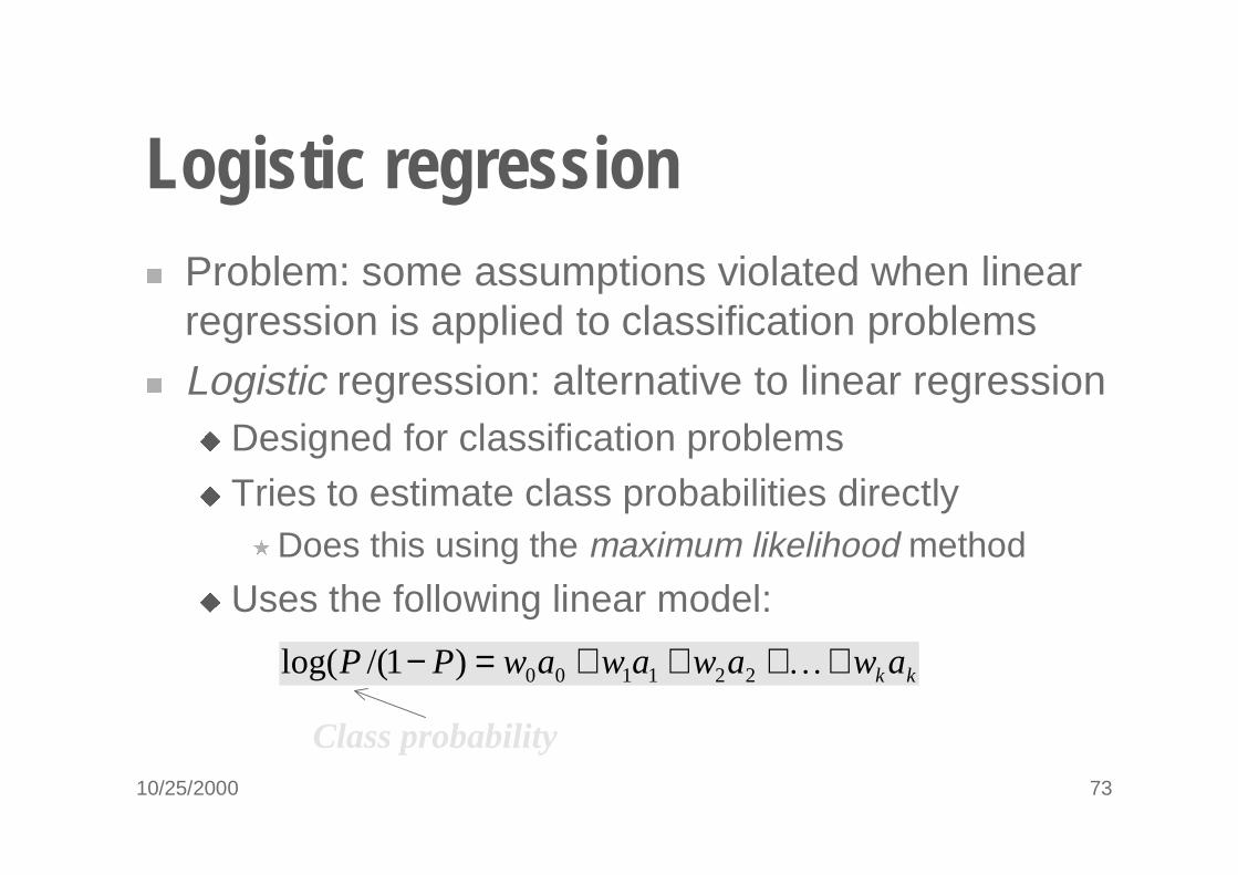
Logistic regression� Problem: some assumptions violated when linear

regression is applied to classification problems� Logistic regression: alternative to linear regression

� Designed for classification problems� Tries to estimate class probabilities directly

�Does this using the maximum likelihood method

� Uses the following linear model:

kk awawawawPP ++++=− �221100)1/(log(

Class probability

10/25/2000 74

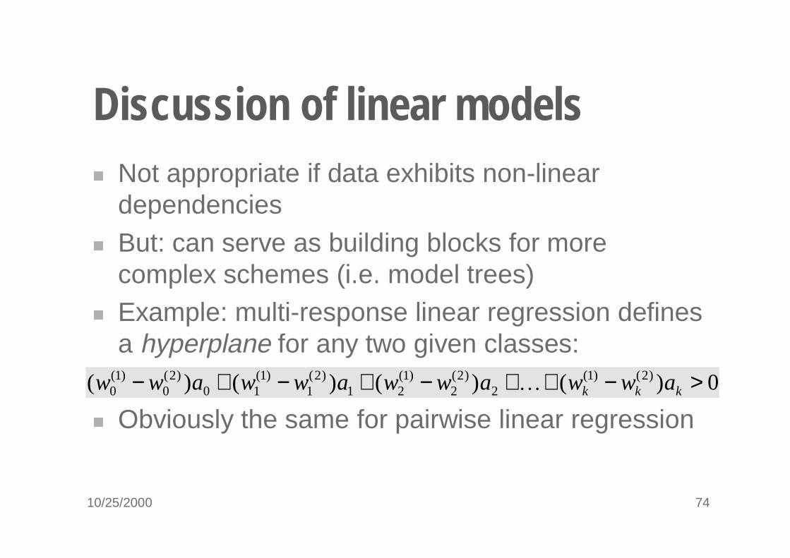
Discussion of linear models� Not appropriate if data exhibits non-linear

dependencies� But: can serve as building blocks for more

complex schemes (i.e. model trees)� Example: multi-response linear regression defines

a hyperplane for any two given classes:

� Obviously the same for pairwise linear regression

0)()()()( )2()1(2

)2(2

)1(21

)2(1

)1(10

)2(0

)1(0 >−++−+−+− kkk awwawwawwaww �

10/25/2000 75

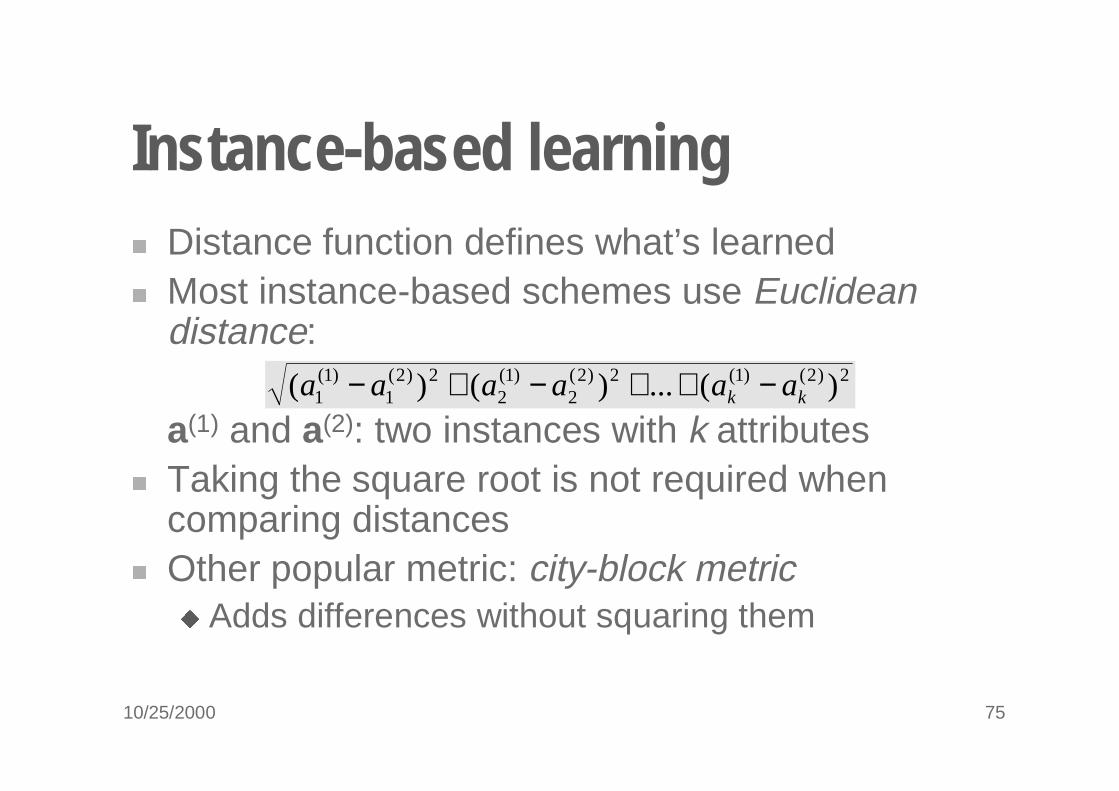
Instance-based learning� Distance function defines what’s learned� Most instance-based schemes use Euclidean

distance:

a(1) and a(2): two instances with k attributes� Taking the square root is not required when

comparing distances� Other popular metric: city-block metric

� Adds differences without squaring them

2)2()1(2)2(2

)1(2

2)2(1

)1(1 )(...)()( kk aaaaaa −++−+−

10/25/2000 76

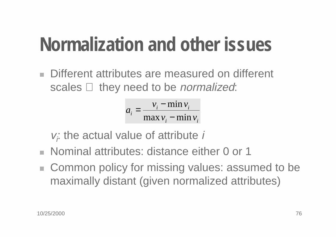
Normalization and other issues� Different attributes are measured on different

scales ⇒ they need to be normalized:

vi: the actual value of attribute i� Nominal attributes: distance either 0 or 1� Common policy for missing values: assumed to be

maximally distant (given normalized attributes)

ii

iii vv

vva

minmaxmin−

−=

10/25/2000 77

Discussion of 1-NN� Often very accurate but also slow: simple version

scans entire training data to derive a prediction� Assumes all attributes are equally important

� Remedy: attribute selection or weights� Possible remedies against noisy instances:

� Taking a majority vote over the k nearest neighbors� Removing noisy instances from dataset (difficult!)

� Statisticians have used k-NN since early 1950s� If n → ∞ and k/n → 0, error approaches minimum

10/25/2000 78

Comments on basic methods� Bayes’ rule stems from his “Essay towards solving

a problem in the doctrine of chances” (1763)� Difficult bit: estimating prior probabilities� Prior-free analysis generates confidence intervals

� Extension of Naïve Bayes: Bayesian Networks� Algorithm for association rules is called APRIORI� Minsky and Papert (1969) showed that linear

classifiers have limitations, e.g. can’t learn XOR� But: combinations of them can (→Neural Networks)

machine learning techniques for data miningtaghi/classes/cap6673/book/ml_part_iv.pdfmachine learning...

Documents