machine learning for the quantified self€¢ prediction of unknown values using the traditional...
TRANSCRIPT
Machine Learning for the Quantified Self
Lecture 7 Reinforcement Learning
Overview
• We have been talking data and making predictions
• What if we want to influence the user? • What intervention/action should we select? • We can use reinforcement learning to figure
this out – Note: not widespread in terms of applications for
the quantified self yet – We discuss the basics, but many improvements
have been made over the years
2
Basics of Reinforcement Learning (1)
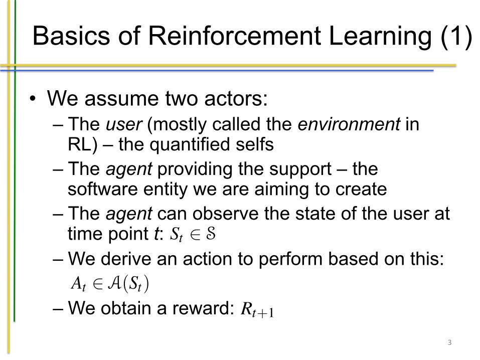
• We assume two actors: – The user (mostly called the environment in
RL) – the quantified selfs – The agent providing the support – the
software entity we are aiming to create – The agent can observe the state of the user at
time point t: – We derive an action to perform based on this:
– We obtain a reward: 3
202 9 Reinforcement Learning to Provide Feedback and Support
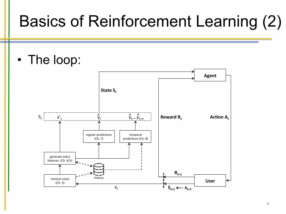
selfers, while the agent is a software entity that decides when and how to supporta user (e.g. the app running on the mobile phone). The agent can observe the stateof the user at a certain time point t, denoted as St 2 S. Connecting to our previouschapters we make the definition of this state a bit more precise. We obtain a datainstance xt from the user at time t that represents the sensor values. We then applythe techniques we have previously discussed to create a representation of the stateof the user based on this sensory data. This includes:
• Removal of noise (cf. Chapter 3).• Enrichment of our original set of features without noise by additional ones (fol-
lowing Chapter 4 and the presence in a certain cluster as explained in Chapter 5),resulting in an enriched set x0t
• Prediction of unknown values using the traditional machine learning techniquesexplained in Chapter 7: yt
• Prediction of unknown (future) values using the machine learning techniquesexplained in Chapter 8, resulting in yt , . . . , yt+n if n time points in the future arepredicted. Note that making predictions for the future can be tricky as we nowintend to influence the future by intervening. We will return to this discussionlater.
removenoise(Ch.3)
generateextrafeatures(Ch.4/5)
regularpredic=ons(Ch.7)
temporalpredic=ons(Ch.8)
x’t yt yt,…yt+nSt
Agent
User
StateSt
RewardRt
xt
Ac0onAt
St+1xt+1
Rt+1
^ ^ ^
history
Fig. 9.1: Our quantified self approach as a Reinforcement Learning Problem (RLloop from [101])
For some approaches we might require a history of measurements (e.g. temporalfeatures and predictions), indicated by the database and dashed arrows in the figure.Together these values form our state St . Based on St the agent can make a decision
9.1 Basic Setting 203
on a certain action At , taken from the set of available actions in the current state, i.e.At 2 A(St). The applied action results in a new state of the user (St+1 obtained viaprocessing xt+1) and a so-called reward Rt+1. The reward is the goal in reinforce-ment learning problems. It can be defined based on the state of the user and maps itto a numerical value. For instance, the overall state of happiness of Bruce at a certaintime point. We are not only interested in the next reward we obtain, but in the totalrewards we expect to accumulate in the future, called a value function. An action tosupport Bruce might for example not have an immediate effect while it does turn outto be best in terms of future rewards. In reinforcement learning we try to find whatis called a policy, expressing which action to perform in what state. Policies aredeemed suitable when the application of the policy results in a lot of rewards overtime (i.e. we perform well in terms of the value function). Approaches should strikea good balance between exploration (trying out new actions to see how successfulthey are) and exploitation (applying known successful actions). If we perform toolittle exploration we might never perform a potentially very successful action whileif we never exploit we could end up trying actions that are not appropriate all thetime.
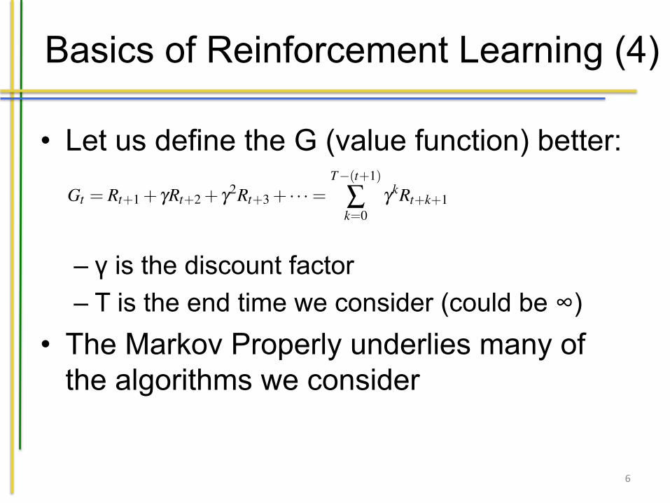
Let us formulate the problem we are facing a bit more precise and formal (yes,expect a good number of formulae to follow shortly). We define the goal Gt at timepoint t by means of the future reward we obtain:
Gt = Rt+1 + gRt+2 + g2Rt+3 + · · ·=T�(t+1)
Âk=0
gkRt+k+1 (9.1)
Here, g is a discount factor for the future reward in the range [0,1]. It indicatesthe relevance of these for the evaluation. T expresses the end time we consider inour system (which can also be •). In case of a value g = 0 we only care aboutthe immediate reward while for a value of g = 1 we care about all future rewards.One important aspect in several approaches we will discuss is that the system wedescribed in Figure 9.1 has the Markov Property. To define this property in a formalway, let us consider our states and rewards. We can express a certain probability thatwe end up in a state St+1 = s with a reward Rt+1 = r based on our entire history:
Pr{Rt+1 = r,St+1 = s|S0,A0,R0, . . . ,St ,At ,Rt} (9.2)
We can also only consider the history of the previous time point without consideringthe reward at the time point:
Pr{Rt+1 = r,St+1 = s|St ,At} (9.3)
We say that the state property has the Markov Property when both probabilities areequal for all rewards r and states s over all time points. In order words, when theprevious state and action contain enough information to assess the probabilities of
9.1 Basic Setting 203
on a certain action At , taken from the set of available actions in the current state, i.e.At 2 A(St). The applied action results in a new state of the user (St+1 obtained viaprocessing xt+1) and a so-called reward Rt+1. The reward is the goal in reinforce-ment learning problems. It can be defined based on the state of the user and maps itto a numerical value. For instance, the overall state of happiness of Bruce at a certaintime point. We are not only interested in the next reward we obtain, but in the totalrewards we expect to accumulate in the future, called a value function. An action tosupport Bruce might for example not have an immediate effect while it does turn outto be best in terms of future rewards. In reinforcement learning we try to find whatis called a policy, expressing which action to perform in what state. Policies aredeemed suitable when the application of the policy results in a lot of rewards overtime (i.e. we perform well in terms of the value function). Approaches should strikea good balance between exploration (trying out new actions to see how successfulthey are) and exploitation (applying known successful actions). If we perform toolittle exploration we might never perform a potentially very successful action whileif we never exploit we could end up trying actions that are not appropriate all thetime.
Let us formulate the problem we are facing a bit more precise and formal (yes,expect a good number of formulae to follow shortly). We define the goal Gt at timepoint t by means of the future reward we obtain:
Gt = Rt+1 + gRt+2 + g2Rt+3 + · · ·=T�(t+1)
Âk=0
gkRt+k+1 (9.1)
Here, g is a discount factor for the future reward in the range [0,1]. It indicatesthe relevance of these for the evaluation. T expresses the end time we consider inour system (which can also be •). In case of a value g = 0 we only care aboutthe immediate reward while for a value of g = 1 we care about all future rewards.One important aspect in several approaches we will discuss is that the system wedescribed in Figure 9.1 has the Markov Property. To define this property in a formalway, let us consider our states and rewards. We can express a certain probability thatwe end up in a state St+1 = s with a reward Rt+1 = r based on our entire history:
Pr{Rt+1 = r,St+1 = s|S0,A0,R0, . . . ,St ,At ,Rt} (9.2)
We can also only consider the history of the previous time point without consideringthe reward at the time point:
Pr{Rt+1 = r,St+1 = s|St ,At} (9.3)
We say that the state property has the Markov Property when both probabilities areequal for all rewards r and states s over all time points. In order words, when theprevious state and action contain enough information to assess the probabilities of
Basics of Reinforcement Learning (2)
• The loop:
4
202 9 Reinforcement Learning to Provide Feedback and Support
selfers, while the agent is a software entity that decides when and how to supporta user (e.g. the app running on the mobile phone). The agent can observe the stateof the user at a certain time point t, denoted as St 2 S. Connecting to our previouschapters we make the definition of this state a bit more precise. We obtain a datainstance xt from the user at time t that represents the sensor values. We then applythe techniques we have previously discussed to create a representation of the stateof the user based on this sensory data. This includes:
• Removal of noise (cf. Chapter 3).• Enrichment of our original set of features without noise by additional ones (fol-
lowing Chapter 4 and the presence in a certain cluster as explained in Chapter 5),resulting in an enriched set x0t
• Prediction of unknown values using the traditional machine learning techniquesexplained in Chapter 7: yt
• Prediction of unknown (future) values using the machine learning techniquesexplained in Chapter 8, resulting in yt , . . . , yt+n if n time points in the future arepredicted. Note that making predictions for the future can be tricky as we nowintend to influence the future by intervening. We will return to this discussionlater.
removenoise(Ch.3)
generateextrafeatures(Ch.4/5)
regularpredic=ons(Ch.7)
temporalpredic=ons(Ch.8)
x’t yt yt,…yt+nSt
Agent
User
StateSt
RewardRt
xt
Ac0onAt
St+1xt+1
Rt+1
^ ^ ^
history
Fig. 9.1: Our quantified self approach as a Reinforcement Learning Problem (RLloop from [101])
For some approaches we might require a history of measurements (e.g. temporalfeatures and predictions), indicated by the database and dashed arrows in the figure.Together these values form our state St . Based on St the agent can make a decision
Basics of Reinforcement Learning (3)
• We do not strive for immediate reward only, but rewards we accumulate in the future, called the value function
• A policy maps a state to an action (when to do what)
• We should balance exploration and exploitation
5
Basics of Reinforcement Learning (4)
• Let us define the G (value function) better:
– γ is the discount factor – T is the end time we consider (could be ∞)
• The Markov Properly underlies many of the algorithms we consider
6
9.1 Basic Setting 203
on a certain action At , taken from the set of available actions in the current state, i.e.At 2 A(St). The applied action results in a new state of the user (St+1 obtained viaprocessing xt+1) and a so-called reward Rt+1. The reward is the goal in reinforce-ment learning problems. It can be defined based on the state of the user and maps itto a numerical value. For instance, the overall state of happiness of Bruce at a certaintime point. We are not only interested in the next reward we obtain, but in the totalrewards we expect to accumulate in the future, called a value function. An action tosupport Bruce might for example not have an immediate effect while it does turn outto be best in terms of future rewards. In reinforcement learning we try to find whatis called a policy, expressing which action to perform in what state. Policies aredeemed suitable when the application of the policy results in a lot of rewards overtime (i.e. we perform well in terms of the value function). Approaches should strikea good balance between exploration (trying out new actions to see how successfulthey are) and exploitation (applying known successful actions). If we perform toolittle exploration we might never perform a potentially very successful action whileif we never exploit we could end up trying actions that are not appropriate all thetime.
Let us formulate the problem we are facing a bit more precise and formal (yes,expect a good number of formulae to follow shortly). We define the goal Gt at timepoint t by means of the future reward we obtain:
Gt = Rt+1 + gRt+2 + g2Rt+3 + · · ·=T�(t+1)
Âk=0
gkRt+k+1 (9.1)
Here, g is a discount factor for the future reward in the range [0,1]. It indicatesthe relevance of these for the evaluation. T expresses the end time we consider inour system (which can also be •). In case of a value g = 0 we only care aboutthe immediate reward while for a value of g = 1 we care about all future rewards.One important aspect in several approaches we will discuss is that the system wedescribed in Figure 9.1 has the Markov Property. To define this property in a formalway, let us consider our states and rewards. We can express a certain probability thatwe end up in a state St+1 = s with a reward Rt+1 = r based on our entire history:
Pr{Rt+1 = r,St+1 = s|S0,A0,R0, . . . ,St ,At ,Rt} (9.2)
We can also only consider the history of the previous time point without consideringthe reward at the time point:
Pr{Rt+1 = r,St+1 = s|St ,At} (9.3)
We say that the state property has the Markov Property when both probabilities areequal for all rewards r and states s over all time points. In order words, when theprevious state and action contain enough information to assess the probabilities of

Markov Property
• We can express a probability of ending up in a state with a reward based on the entire history:
• We can also define it based on the previous state and action only:
• If the probabilities are equal we satisfy the property • True for the quantified self?
7
9.1 Basic Setting 203
on a certain action At , taken from the set of available actions in the current state, i.e.At 2 A(St). The applied action results in a new state of the user (St+1 obtained viaprocessing xt+1) and a so-called reward Rt+1. The reward is the goal in reinforce-ment learning problems. It can be defined based on the state of the user and maps itto a numerical value. For instance, the overall state of happiness of Bruce at a certaintime point. We are not only interested in the next reward we obtain, but in the totalrewards we expect to accumulate in the future, called a value function. An action tosupport Bruce might for example not have an immediate effect while it does turn outto be best in terms of future rewards. In reinforcement learning we try to find whatis called a policy, expressing which action to perform in what state. Policies aredeemed suitable when the application of the policy results in a lot of rewards overtime (i.e. we perform well in terms of the value function). Approaches should strikea good balance between exploration (trying out new actions to see how successfulthey are) and exploitation (applying known successful actions). If we perform toolittle exploration we might never perform a potentially very successful action whileif we never exploit we could end up trying actions that are not appropriate all thetime.
Let us formulate the problem we are facing a bit more precise and formal (yes,expect a good number of formulae to follow shortly). We define the goal Gt at timepoint t by means of the future reward we obtain:
Gt = Rt+1 + gRt+2 + g2Rt+3 + · · ·=T�(t+1)
Âk=0
gkRt+k+1 (9.1)
Here, g is a discount factor for the future reward in the range [0,1]. It indicatesthe relevance of these for the evaluation. T expresses the end time we consider inour system (which can also be •). In case of a value g = 0 we only care aboutthe immediate reward while for a value of g = 1 we care about all future rewards.One important aspect in several approaches we will discuss is that the system wedescribed in Figure 9.1 has the Markov Property. To define this property in a formalway, let us consider our states and rewards. We can express a certain probability thatwe end up in a state St+1 = s with a reward Rt+1 = r based on our entire history:
Pr{Rt+1 = r,St+1 = s|S0,A0,R0, . . . ,St ,At ,Rt} (9.2)
We can also only consider the history of the previous time point without consideringthe reward at the time point:
Pr{Rt+1 = r,St+1 = s|St ,At} (9.3)
We say that the state property has the Markov Property when both probabilities areequal for all rewards r and states s over all time points. In order words, when theprevious state and action contain enough information to assess the probabilities of
MDP (1)
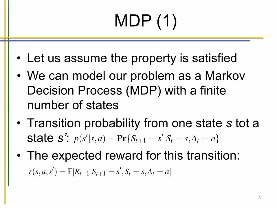
• Let us assume the property is satisfied • We can model our problem as a Markov
Decision Process (MDP) with a finite number of states
• Transition probability from one state s tot a state s’:
• The expected reward for this transition:
8
204 9 Reinforcement Learning to Provide Feedback and Support
moving to a next state properly. If we think of a game of chess, this property is sat-isfied if we know all the pieces on the board and the movement of one piece as thatis all information that is relevant for the game, the entire history is not. Is the prop-erty likely to hold for the quantified self? Good question, which highly depends onthe amount of sensory data obtained, and the problem we aim to tackle. It is highlylikely that it will not be satisfied for quite some cases. A lot of approaches do makethis assumption though, and they often consider the problem as a finite Markov de-cision process (finite MDP) with the hefty assumption of a finite number of statesand actions. Given our input space (where we typically have lots of numerical val-ues) we cannot expect this for our case, but there are ways around this, namely tomap our space to finite domains. We will turn to this later.
Assuming our problem to be a finite MDP though, we define the probability ofmoving to a next state s0 from a state s with action a, referred to as the transitionprobability:
p(s0|s,a) = Pr{St+1 = s0|St = s,At = a} (9.4)
We express the expected reward:
r(s,a,s0) = E[Rt+1|St+1 = s0,St = s,At = a] (9.5)
This formulates our problem in a very nice way. To give a concrete example,of p(s0|s,a) imagine Bruce in a depressed state, we provide Bruce with a message”cheer up” and predict the probability that Bruce will not longer be depressed atthe next time step. Furthermore, we calculate the expected reward r(s,a,s0) for thatoutcome, which will be high as we move to a non-depressed state.
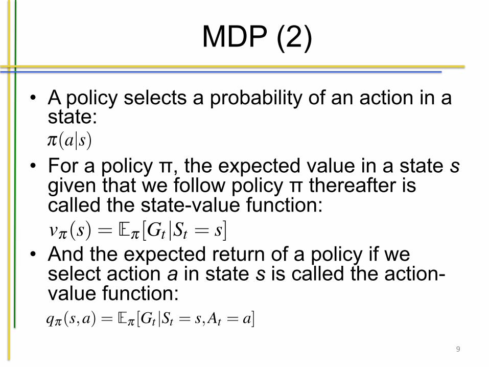
The final aspect we need to fully formulate our problem is the policy p , i.e.when to perform what action. Each policy assigns a probability to a certain availableaction a in a given state s: p(a|s). Given the assumptions we have previously made,the expected value of our policy p in a state s would then be:
vp(s) = Ep [Gt |St = s] (9.6)
And we define the expected return of our policy p after having selected an action ain state s first:
qp(s,a) = Ep [Gt |St = s,At = a] (9.7)
We are interested in finding the policy (or policies) p⇤ that provides the highest valuein all states:
204 9 Reinforcement Learning to Provide Feedback and Support
moving to a next state properly. If we think of a game of chess, this property is sat-isfied if we know all the pieces on the board and the movement of one piece as thatis all information that is relevant for the game, the entire history is not. Is the prop-erty likely to hold for the quantified self? Good question, which highly depends onthe amount of sensory data obtained, and the problem we aim to tackle. It is highlylikely that it will not be satisfied for quite some cases. A lot of approaches do makethis assumption though, and they often consider the problem as a finite Markov de-cision process (finite MDP) with the hefty assumption of a finite number of statesand actions. Given our input space (where we typically have lots of numerical val-ues) we cannot expect this for our case, but there are ways around this, namely tomap our space to finite domains. We will turn to this later.
Assuming our problem to be a finite MDP though, we define the probability ofmoving to a next state s0 from a state s with action a, referred to as the transitionprobability:
p(s0|s,a) = Pr{St+1 = s0|St = s,At = a} (9.4)
We express the expected reward:
r(s,a,s0) = E[Rt+1|St+1 = s0,St = s,At = a] (9.5)
This formulates our problem in a very nice way. To give a concrete example,of p(s0|s,a) imagine Bruce in a depressed state, we provide Bruce with a message”cheer up” and predict the probability that Bruce will not longer be depressed atthe next time step. Furthermore, we calculate the expected reward r(s,a,s0) for thatoutcome, which will be high as we move to a non-depressed state.
The final aspect we need to fully formulate our problem is the policy p , i.e.when to perform what action. Each policy assigns a probability to a certain availableaction a in a given state s: p(a|s). Given the assumptions we have previously made,the expected value of our policy p in a state s would then be:
vp(s) = Ep [Gt |St = s] (9.6)
And we define the expected return of our policy p after having selected an action ain state s first:
qp(s,a) = Ep [Gt |St = s,At = a] (9.7)
We are interested in finding the policy (or policies) p⇤ that provides the highest valuein all states:
MDP (2)
• A policy selects a probability of an action in a state:
• For a policy π, the expected value in a state s
given that we follow policy π thereafter is called the state-value function:
• And the expected return of a policy if we select action a in state s is called the action-value function:
9
204 9 Reinforcement Learning to Provide Feedback and Support
moving to a next state properly. If we think of a game of chess, this property is sat-isfied if we know all the pieces on the board and the movement of one piece as thatis all information that is relevant for the game, the entire history is not. Is the prop-erty likely to hold for the quantified self? Good question, which highly depends onthe amount of sensory data obtained, and the problem we aim to tackle. It is highlylikely that it will not be satisfied for quite some cases. A lot of approaches do makethis assumption though, and they often consider the problem as a finite Markov de-cision process (finite MDP) with the hefty assumption of a finite number of statesand actions. Given our input space (where we typically have lots of numerical val-ues) we cannot expect this for our case, but there are ways around this, namely tomap our space to finite domains. We will turn to this later.
Assuming our problem to be a finite MDP though, we define the probability ofmoving to a next state s0 from a state s with action a, referred to as the transitionprobability:
p(s0|s,a) = Pr{St+1 = s0|St = s,At = a} (9.4)
We express the expected reward:
r(s,a,s0) = E[Rt+1|St+1 = s0,St = s,At = a] (9.5)
This formulates our problem in a very nice way. To give a concrete example,of p(s0|s,a) imagine Bruce in a depressed state, we provide Bruce with a message”cheer up” and predict the probability that Bruce will not longer be depressed atthe next time step. Furthermore, we calculate the expected reward r(s,a,s0) for thatoutcome, which will be high as we move to a non-depressed state.
The final aspect we need to fully formulate our problem is the policy p , i.e.when to perform what action. Each policy assigns a probability to a certain availableaction a in a given state s: p(a|s). Given the assumptions we have previously made,the expected value of our policy p in a state s would then be:
vp(s) = Ep [Gt |St = s] (9.6)
And we define the expected return of our policy p after having selected an action ain state s first:
qp(s,a) = Ep [Gt |St = s,At = a] (9.7)
We are interested in finding the policy (or policies) p⇤ that provides the highest valuein all states:
MDP (3)
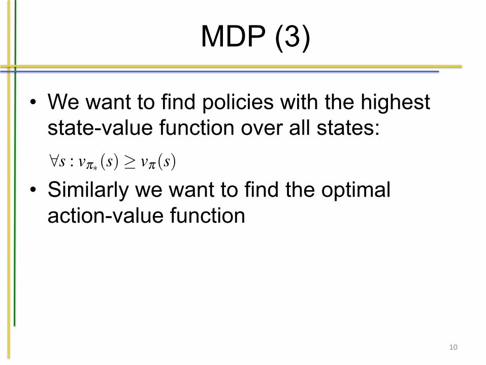
• We want to find policies with the highest state-value function over all states:
• Similarly we want to find the optimal action-value function
10
9.1 Basic Setting 205
8s : vp⇤(s)� vp(s) (9.8)
The value is denoted as v⇤(s). Similarly, we define the optimal value function:q⇤(s,a) given our optimal policies p⇤. Well, the stage is set. We have treated allthe fundamentals.
Fig. 9.2: Example Reinforcement Learning Problem for Bruce
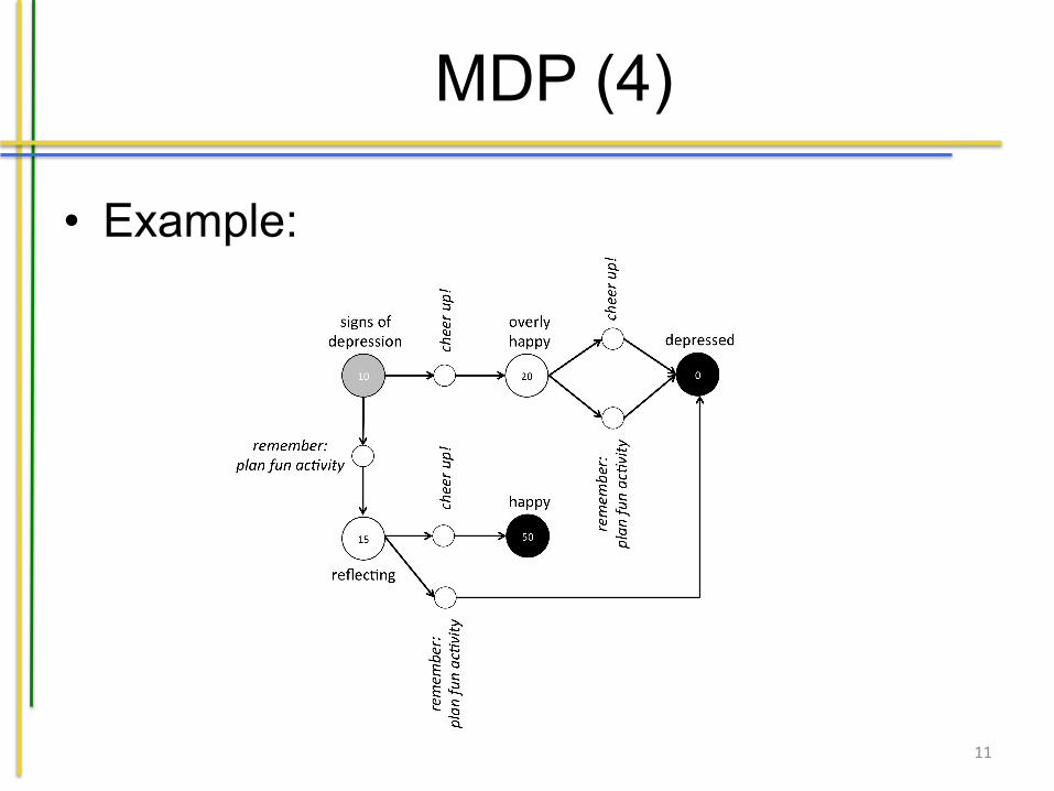
Let us consider a simple example to understand matters a bit better. Figure 9.2shows such an example. We assume that the state resulting from an action is com-pletely deterministic in this case. The figure shows an overview of the relevant statesof Bruce (i.e. S) related to his depression problem. They are presented by the largecircles. We have an initial state (signs of depression), two intermediate states (overlyhappy and reflecting) and two terminal states: depressed and happy. Obviously wedo not mean Bruce will cease to exist when he falls into a depression, but givenhis history he will likely be advised to seek human counseling which is beyond thescope of our system. In a happy state there is no need to support Bruce any longeruntil our friend shows signs of depression yet again. In each state, we have the sametwo actions at our disposal (A(S) is the same for all S 2 S). The first action asksBruce to remember to plan fun activities, something he should recollect from priortherapies. The second option is to give Bruce a boast by providing him the messagecheep up!. The figure expresses the transitions between states based on these actionsby means of arrows with a small circle representing the action, e.g. when we per-form the action cheer up! in the signs of depression state, Bruce moves to the overlyhappy state. Each state also shows the reward it gives. What would be the optimal
MDP (4)
• Example:
11
9.1 Basic Setting 205
8s : vp⇤(s)� vp(s) (9.8)
The value is denoted as v⇤(s). Similarly, we define the optimal action-value function:q⇤(s,a) given our optimal policies p⇤. Well, the stage is set. We have treated all thefundamentals.
Fig. 9.2: Example Reinforcement Learning Problem for Bruce
Let us consider a simple example to understand matters a bit better. Figure 9.2shows such an example. We assume that the state resulting from an action is com-pletely deterministic in this case. The figure shows an overview of the relevant statesof Bruce (i.e. S) related to his depression problem. They are presented by the largecircles. We have an initial state (signs of depression), two intermediate states (overlyhappy and reflecting) and two terminal states: depressed and happy. Obviously wedo not mean Bruce will cease to exist when he falls into a depression, but givenhis history he will likely be advised to seek human counseling which is beyond thescope of our system. In a happy state there is no need to support Bruce any longeruntil our friend shows signs of depression yet again. In each state, we have the sametwo actions at our disposal (A(S) is the same for all S 2 S). The first action asksBruce to remember to plan fun activities, something he should recollect from priortherapies. The second option is to give Bruce a boast by providing him the messagecheep up!. The figure expresses the transitions between states based on these actionsby means of arrows with a small circle representing the action, e.g. when we per-form the action cheer up! in the signs of depression state, Bruce moves to the overlyhappy state. Each state also shows the reward it gives. What would be the optimal
One Step Sarsa (1)
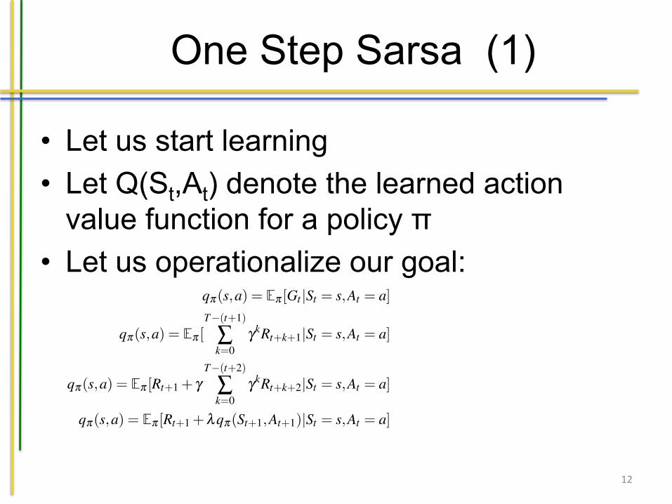
• Let us start learning • Let Q(St,At) denote the learned action
value function for a policy π • Let us operationalize our goal:
12
206 9 Reinforcement Learning to Provide Feedback and Support
policy for our initial state in this case? Well, assuming that we only consider thereward of the next state it would be selecting cheer up! resulting in the highest im-mediate reward of 20. In the long run however (if we only look ahead one additionaltime point) the obvious choice is to select remember: plan fun activity as we can getBruce in the happy state after one more action then. Now how do we find such apolicy p? We will look into that now.
9.2 One-Step Sarsa Temporal Difference Learning
In the first approach we are going to discuss we assume that we can make a tableof the situations versus the possible actions. This algorithm is based on [94]. Wedo not assume complete knowledge on the environment making the temporal differ-ence based approach most suitable. It allows for online learning (i.e learning fromexperiences as we go along) while still using information we obtained in the past.Our goal is to learn a policy that gives us appropriate actions given a certain state,also called a control problem. An alternative is to learn the valuing of a state (whichwe will not consider in the remainder of this chapter). Let Q(St ,At) denote the valueof the state-action pair for a policy p . This represents how appropriate action At isin situation St given our policy p , i.e. how suitable a transition is between states.For instance, how appropriate the action to say ”cheer up” for a depressed Bruce is.Remember that we have previously defined qp(s,a). We can alter this definition abit, by saying that instead of looking at the goal G(t) (i.e. the future rewards), welook at the reward we obtain in the next state and the state-action value of our policygiven the next state. We derive a new definition as follows:
qp(s,a) = Ep [Gt |St = s,At = a] (9.9)
qp(s,a) = Ep [T�(t+1)
Âk=0
gkRt+k+1|St = s,At = a] (9.10)
qp(s,a) = Ep [Rt+1 + gT�(t+2)
Âk=0
gkRt+k+2|St = s,At = a] (9.11)
qp(s,a) = Ep [Rt+1 +lqp(St+1,At+1)|St = s,At = a] (9.12)
We want to create an estimate of the value of an action At in a situation St given ourpolicy p . We define this estimate as Q(St ,At). Based on our previous derivation wedefine Q(St ,At) as:
Q(St ,At) Q(St ,At)+a(Rt+1 + gQ(St+1,At+1)�Q(St ,At)) (9.13)
One Step Sarsa (2)
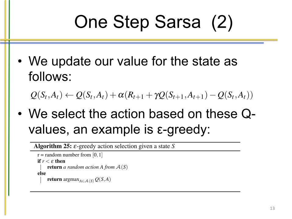
• We update our value for the state as follows:
• We select the action based on these Q-values, an example is ε-greedy:
13
206 9 Reinforcement Learning to Provide Feedback and Support
policy for our initial state in this case? Well, assuming that we only consider thereward of the next state it would be selecting cheer up! resulting in the highest im-mediate reward of 20. In the long run however (if we only look ahead one additionaltime point) the obvious choice is to select remember: plan fun activity as we can getBruce in the happy state after one more action then. Now how do we find such apolicy p? We will look into that now.
9.2 One-Step Sarsa Temporal Difference Learning
In the first approach we are going to discuss we assume that we can make a tableof the situations versus the possible actions. This algorithm is based on [94]. Wedo not assume complete knowledge on the environment making the temporal differ-ence based approach most suitable. It allows for online learning (i.e learning fromexperiences as we go along) while still using information we obtained in the past.Our goal is to learn a policy that gives us appropriate actions given a certain state,also called a control problem. An alternative is to learn the valuing of a state (whichwe will not consider in the remainder of this chapter). Let Q(St ,At) denote the valueof the state-action pair for a policy p . This represents how appropriate action At isin situation St given our policy p , i.e. how suitable a transition is between states.For instance, how appropriate the action to say ”cheer up” for a depressed Bruce is.Remember that we have previously defined qp(s,a). We can alter this definition abit, by saying that instead of looking at the goal G(t) (i.e. the future rewards), welook at the reward we obtain in the next state and the state-action value of our policygiven the next state. We derive a new definition as follows:
qp(s,a) = Ep [Gt |St = s,At = a] (9.9)
qp(s,a) = Ep [T�(t+1)
Âk=0
gkRt+k+1|St = s,At = a] (9.10)
qp(s,a) = Ep [Rt+1 + gT�(t+2)
Âk=0
gkRt+k+2|St = s,At = a] (9.11)
qp(s,a) = Ep [Rt+1 +lqp(St+1,At+1)|St = s,At = a] (9.12)
We want to create an estimate of the value of an action At in a situation St given ourpolicy p . We define this estimate as Q(St ,At). Based on our previous derivation wedefine Q(St ,At) as:
Q(St ,At) Q(St ,At)+a(Rt+1 + gQ(St+1,At+1)�Q(St ,At)) (9.13)
9.2 One-Step Sarsa Temporal Difference Learning 207
This expresses that the new value for an state-action pair is the old value plus afactor a times the difference between the reward at the next time step and the valueof the next state-action pair with the old state-action pair value.
Once we have these values for a policy p we still need to decide on what actionA 2 A(St) to select. Various action selection approaches are available, includingone called e-greedy. In the e-greedy approach we select a random action with prob-ability e to allow for exploration, while in all other cases we select the action withthe highest value. This is formalized in Algorithm 25.
Algorithm 25: e-greedy action selection given a state Sr = random number from [0,1]if r < e then
return a random action A from A(S)else
return argmaxA2A(S) Q(S,A)
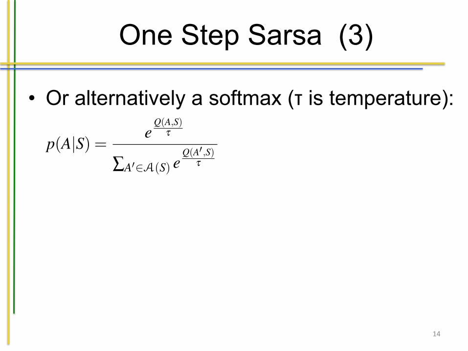
An alternative action selection mechanism is the softmax approach. The probabilityof selecting an actions A in situation S is defined as:
p(A|S) = eQ(A,S)
t
ÂA02A(S) eQ(A0 ,S)
t
(9.14)
Here, t expresses a temperature, similar to simulated annealing that we have treatedbefore. t has a value > 0. The lower the temperature, the more we select based onthe value for Q(A,S). The higher, the more we select in a random way. We can startwith a high temperature (doing more exploration) and lower the temperature as wegather more experiences (exploitation).
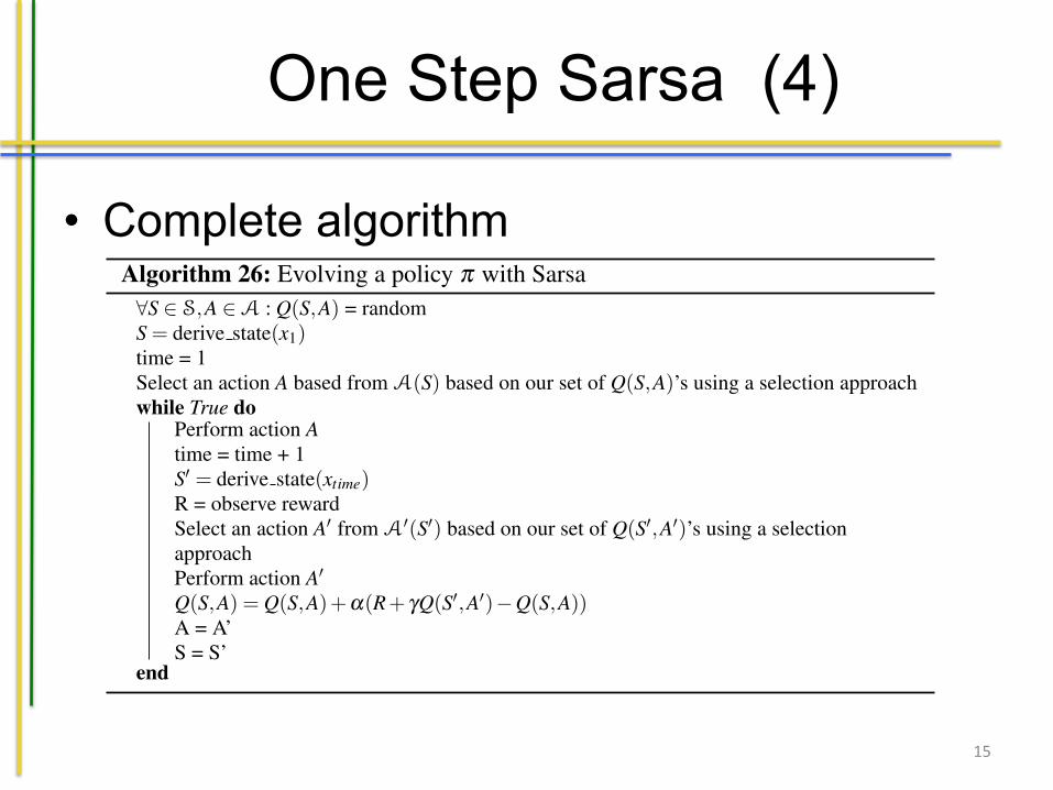
Given the selection method, we will explain the Sarsa algorithm to adjust thepolicy (note that we leave out some details with respect to the Markov model for thesake of simplicity). The algorithm is shown in Algorithm 26. We randomly assigna value for Q(S,A) in the initial phase. We start by deriving the state S from ourinitial set of sensory values x1 and select an action based on some action selectionmechanism and our values for all actions given the situation Q(S,A). We performthe action, and collect sensory data again to form state S0. We also observe the re-ward R. In this new situation, we select a next action A0. We can now update ourvalue of Q(S,A). We set the action A to our new action A0, the situation S to S0 andcontinue in our loop by executing the action, observing the new situation S0, etcetera.
Let us return to our previous example of Bruce. We eventually end up with theQ-values shown in Table 9.1. Note that we only show states where we can perform
One Step Sarsa (3)
• Or alternatively a softmax (τ is temperature):
14
9.2 One-Step Sarsa Temporal Difference Learning 207
This expresses that the new value for an state-action pair is the old value plus afactor a times the difference between the reward at the next time step and the valueof the next state-action pair with the old state-action pair value.
Once we have these values for a policy p we still need to decide on what actionA 2 A(St) to select. Various action selection approaches are available, includingone called e-greedy. In the e-greedy approach we select a random action with prob-ability e to allow for exploration, while in all other cases we select the action withthe highest value. This is formalized in Algorithm 25.
Algorithm 25: e-greedy action selection given a state Sr = random number from [0,1]if r < e then
return a random action A from A(S)else
return argmaxA2A(S) Q(S,A)
An alternative action selection mechanism is the softmax approach. The probabilityof selecting an actions A in situation S is defined as:
p(A|S) = eQ(A,S)
t
ÂA02A(S) eQ(A0 ,S)
t
(9.14)
Here, t expresses a temperature, similar to simulated annealing that we have treatedbefore. t has a value > 0. The lower the temperature, the more we select based onthe value for Q(A,S). The higher, the more we select in a random way. We can startwith a high temperature (doing more exploration) and lower the temperature as wegather more experiences (exploitation).
Given the selection method, we will explain the Sarsa algorithm to adjust thepolicy (note that we leave out some details with respect to the Markov model for thesake of simplicity). The algorithm is shown in Algorithm 26. We randomly assigna value for Q(S,A) in the initial phase. We start by deriving the state S from ourinitial set of sensory values x1 and select an action based on some action selectionmechanism and our values for all actions given the situation Q(S,A). We performthe action, and collect sensory data again to form state S0. We also observe the re-ward R. In this new situation, we select a next action A0. We can now update ourvalue of Q(S,A). We set the action A to our new action A0, the situation S to S0 andcontinue in our loop by executing the action, observing the new situation S0, etcetera.
Let us return to our previous example of Bruce. We eventually end up with theQ-values shown in Table 9.1. Note that we only show states where we can perform
One Step Sarsa (4)
• Complete algorithm
15
208 9 Reinforcement Learning to Provide Feedback and Support
Algorithm 26: Evolving a policy p with Sarsa8S 2 S,A 2A : Q(S,A) = randomS = derive state(x1)time = 1Select an action A based from A(S) based on our set of Q(S,A)’s using a selection approachwhile True do
Perform action Atime = time + 1S0 = derive state(xtime)R = observe rewardSelect an action A0 from A0(S0) based on our set of Q(S0,A0)’s using a selectionapproachPerform action A0
Q(S,A) = Q(S,A)+a(R+ gQ(S0,A0)�Q(S,A))A = A’S = S’
end
Table 9.1: Q(S,A) values for the Bruce case
cheer up! (cu) remember: plan fun ac-tivity (pfa)
signs of depression (sod) 0 50
overly happy (oh) 0 0
reflecting (ref) 50 0
actions, thereby omitting the terminal states. Let us consider one example Q-value,namely Q(sod, p f a) (considering the abbreviations noted in the table). Given ourequation for the Q-values (assuming e �greedy) we compute that:
Q(sod, p f a) = Q(sod, p f a)+a(15+ gQ(re f ,cu)�Q(sod, p f a)) (9.15)
Which results in a value of 50.We now have a simple approach to decide on feedback and support for our quan-
tified selfs. However, more sophistical approaches are present that help to improvethis simple algorithm. We will discuss these next.
9.3 Q-learning
Q-learning is certainly one of the most well-known reinforcement learning ap-proaches and was introduced in [111]. In Q-learning we follow roughly the same
One Step Sarsa (5)
• For Sarsa, we pick our actions in the same way at each step
• This is called on-policy
16
Q-Learning (1)
• For Q-learning, we do not perform the next action before updating our Q-values
• We just assume that we select the highest value in the next state
• Off-policy approach
17
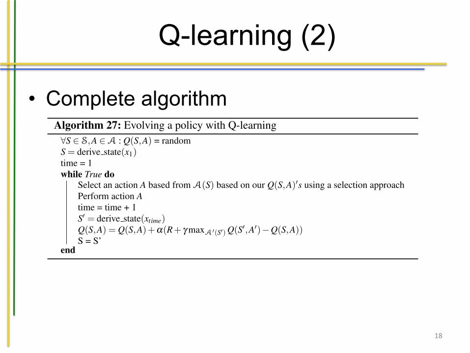
Q-learning (2)
• Complete algorithm
18
9.4 Sarsa(l ) and Q(l ) 209
approaches as we have seen in Sarsa. However, while in Sarsa we updated our val-ues for Q(S,A) based on the value of the selected action in the next state S0 usingthe same policy (e.g. e-greedy), for Q-learning we directly select the action that hasthe highest value for the next state. This simplifies our algorithm, as we can see be-low. The approach is sometimes called off-policy to reflect that we apply a differentpolicy for the calculation of the new value of Q(S,A) compared to the one we useto select the actual action A. Sarsa is an on-policy approach as we use the same forboth cases.
Algorithm 27: Evolving a policy with Q-learning8S 2 S,A 2A : Q(S,A) = randomS = derive state(x1)time = 1while True do
Select an action A based from A(S) based on our Q(S,A)0s using a selection approachPerform action Atime = time + 1S0 = derive state(xtime)Q(S,A) = Q(S,A)+a(R+ g maxA0(S0) Q(S0,A0)�Q(S,A))S = S’
end
9.4 Sarsa(l ) and Q(l )
We are going to extend the approaches we have just considered. In our simple Sarsaand Q-learning approaches we lacked a concept that was able to identify what ac-tions we had taken in the past that contributed to the current state. This would allowus to put blame or credit to those choices we made before instead of just lookingone step forward (hence, our previous name). These are so-called eligibility traces.Assume Zt(s,a) represents the eligibility trace at time point t for state s with actiona. The value for the trace is defined as:
Zt(s,a) =
(glZt�1 +1 if s = St ^a = At
glZt�1 otherwise(9.16)
The combined factors g (as seen before) and l determine how quickly the historyof the eligibility trace decays. We add 1 to the eligibility trace of a state if thestate occurred, and 0 otherwise. How do we incorporate this? Well, we update ourequation for calculating Q(S,A). For Sarsa this becomes:
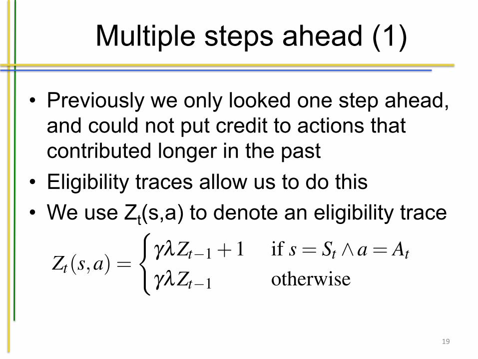
Multiple steps ahead (1)
• Previously we only looked one step ahead, and could not put credit to actions that contributed longer in the past
• Eligibility traces allow us to do this • We use Zt(s,a) to denote an eligibility trace
19
9.4 Sarsa(l ) and Q(l ) 209
approaches as we have seen in Sarsa. However, while in Sarsa we updated our val-ues for Q(S,A) based on the value of the selected action in the next state S0 usingthe same policy (e.g. e-greedy), for Q-learning we directly select the action that hasthe highest value for the next state. This simplifies our algorithm, as we can see be-low. The approach is sometimes called off-policy to reflect that we apply a differentpolicy for the calculation of the new value of Q(S,A) compared to the one we useto select the actual action A. Sarsa is an on-policy approach as we use the same forboth cases.
Algorithm 27: Evolving a policy with Q-learning8S 2 S,A 2A : Q(S,A) = randomS = derive state(x1)time = 1while True do
Select an action A based from A(S) based on our Q(S,A)0s using a selection approachPerform action Atime = time + 1S0 = derive state(xtime)Q(S,A) = Q(S,A)+a(R+ g maxA0(S0) Q(S0,A0)�Q(S,A))S = S’
end
9.4 Sarsa(l ) and Q(l )
We are going to extend the approaches we have just considered. In our simple Sarsaand Q-learning approaches we lacked a concept that was able to identify what ac-tions we had taken in the past that contributed to the current state. This would allowus to put blame or credit to those choices we made before instead of just lookingone step forward (hence, our previous name). These are so-called eligibility traces.Assume Zt(s,a) represents the eligibility trace at time point t for state s with actiona. The value for the trace is defined as:
Zt(s,a) =
(glZt�1 +1 if s = St ^a = At
glZt�1 otherwise(9.16)
The combined factors g (as seen before) and l determine how quickly the historyof the eligibility trace decays. We add 1 to the eligibility trace of a state if thestate occurred, and 0 otherwise. How do we incorporate this? Well, we update ourequation for calculating Q(S,A). For Sarsa this becomes:
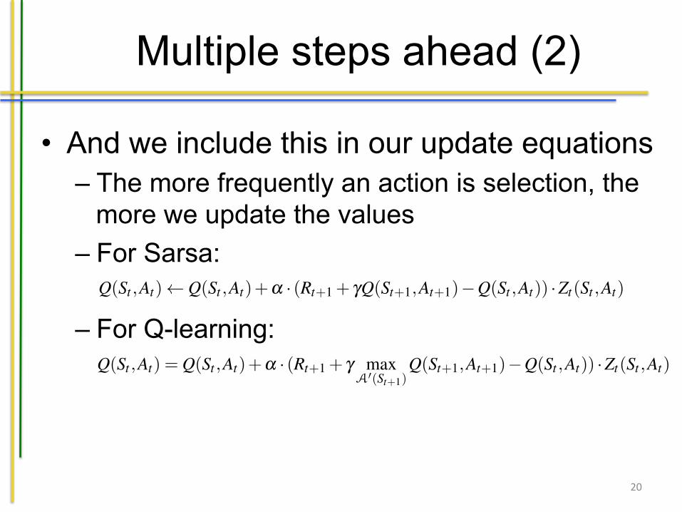
Multiple steps ahead (2)
• And we include this in our update equations – The more frequently an action is selection, the
more we update the values – For Sarsa:
– For Q-learning:
20
210 9 Reinforcement Learning to Provide Feedback and Support
Q(St ,At) Q(St ,At)+a · (Rt+1 + gQ(St+1,At+1)�Q(St ,At)) ·Zt(St ,At) (9.17)
Here, we see that changes in the Q-value depend on the value of the eligibility trace.If the state-action pair is more eligible (i.e. in our history the pair has been appliedmore frequently) the magnitude of the update is increased. We can simply plug thisinto our learning algorithm we have defined before. For Q-learning the new equationbecomes:
Q(St ,At) = Q(St ,At)+a · (Rt+1 + g maxA0(St+1)
Q(St+1,At+1)�Q(St ,At)) ·Zt(St ,At)
(9.18)
9.5 Approximate Solutions
So far we have assumed a value Q(S,A) for each combination, but this is not veryrealistic in our quantified self setting. We are likely to have a lot of different statesand hopefully also have quite some opportunities to provide a form of support orfeedback (in other words: actions). Hence, we somehow need to learn a model thatpredicts the value Q(S,A) in a situation S for a given action A. Well, luckily wehave seen a lot of these models before in our previous chapters. We can see eachobservation of a state S and an action A with a value Q(S,A) as an instance of alearning problem with Q(S,A) as our target. Assume we have a matrix of weightsw that represents a model for our predictions. For instance, the weights of a neuralnetworks. Assuming our model is represented as f (St ,At ,w) giving a prediction forQ(St ,At) we can define the error as:
ÂS2S,A2A
q(Q(S,A)� f (S,A,w))2 (9.19)
In case we do not have instances for all cases we obviously only consider thecases we have information about. We can apply this model to estimate the value forQ(S,A) in our algorithms, and update the model after each state change.
9.6 Discretizing the State Space
One final aspect we will devote some attention to ways to discretize the state space.We could have an infinite state space in our quantified self setting, and we would liketo create useful representations of states. If we just consider all possible values forthe activity level of Arnold we would already be lost with our previous approaches.For this purpose, the U-tree algorithm (cf. [106]) can be used. Note that we slightly
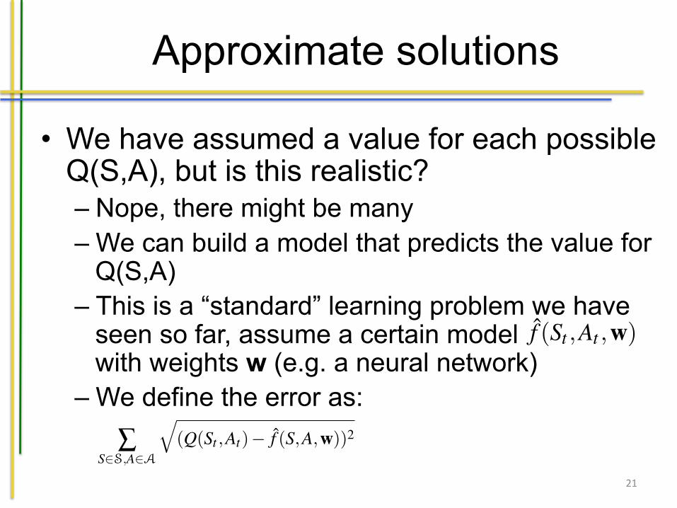
Approximate solutions
• We have assumed a value for each possible Q(S,A), but is this realistic? – Nope, there might be many – We can build a model that predicts the value for
Q(S,A) – This is a “standard” learning problem we have
seen so far, assume a certain model with weights w (e.g. a neural network)
– We define the error as:
21
210 9 Reinforcement Learning to Provide Feedback and Support
Q(St ,At) Q(St ,At)+a · (Rt+1 + gQ(St+1,At+1)�Q(St ,At)) ·Zt(St ,At) (9.17)
Here, we see that changes in the Q-value depend on the value of the eligibility trace.If the state-action pair is more eligible (i.e. in our history the pair has been appliedmore frequently) the magnitude of the update is increased. We can simply plug thisinto our learning algorithm we have defined before. For Q-learning the new equationbecomes:
Q(St ,At) = Q(St ,At)+a · (Rt+1 + g maxA0(St+1)
Q(St+1,At+1)�Q(St ,At)) ·Zt(St ,At)
(9.18)
9.5 Approximate Solutions
So far we have assumed a value Q(S,A) for each combination, but this is not veryrealistic in our quantified self setting. We are likely to have a lot of different statesand hopefully also have quite some opportunities to provide a form of support orfeedback (in other words: actions). Hence, we somehow need to learn a model thatpredicts the value Q(S,A) in a situation S for a given action A. Well, luckily wehave seen a lot of these models before in our previous chapters. We can see eachobservation of a state S and an action A with a value Q(S,A) as an instance of alearning problem with Q(S,A) as our target. Assume we have a matrix of weightsw that represents a model for our predictions. For instance, the weights of a neuralnetworks. Assuming our model is represented as f (St ,At ,w) giving a prediction forQ(St ,At) we can define the error as:
ÂS2S,A2A
q(Q(St ,At)� f (S,A,w))2 (9.19)
In case we do not have instances for all cases we obviously only consider thecases we have information about. We can apply this model to estimate the value forQ(S,A) in our algorithms, and update the model after each state change.
9.6 Discretizing the State Space
One final aspect we will devote some attention to ways to discretize the state space.We could have an infinite state space in our quantified self setting, and we would liketo create useful representations of states. If we just consider all possible values forthe activity level of Arnold we would already be lost with our previous approaches.For this purpose, the U-tree algorithm (cf. [106]) can be used. Note that we slightly
Handling continuous values in the state space (1)
• Final part: – We have states represented by continuous
values, what then? – We have an infinite state space – We need to discretize this – We can use the U-tree algorithm for this purpose
22
Handling continuous values in the state space (2)
• How does it work? – We build a state tree, that maps our continuous values to
a state – We start with a single leaf – We collect data for a while – For all attributes Xi we try different splits based on the
(sorted) values we have collected – We test whether the splits result in a significant difference
in Q-values using the Kolmogorov Smirnov test – We select the attribute with the lowest p-value and split
on it (if below 0.05) – We continue collecting data again and repeat the
procedure per leaf
23