Machine Learning Enhancement of Storm-Scale Ensemble ProbabilisticQuantitative Precipitation Forecasts

DAVID JOHN GAGNE II

School of Meteorology, University of Oklahoma, Norman, Oklahoma

AMY MCGOVERN

School of Computer Science, University of Oklahoma, Norman, Oklahoma

MING XUE

Center for Analysis and Prediction of Storms, and School of Meteorology, University of Oklahoma, Norman, Oklahoma

(Manuscript received 11 September 2013, in final form 25 April 2014)

ABSTRACT

Probabilistic quantitative precipitation forecasts challenge meteorologists due to the wide variability of

precipitation amounts over small areas and their dependence on conditions at multiple spatial and temporal

scales. Ensembles of convection-allowing numerical weather prediction models offer a way to produce im-

proved precipitation forecasts and estimates of the forecast uncertainty. Thesemodels allow for the prediction

of individual convective storms on the model grid, but they often displace the storms in space, time, and

intensity, which results in added uncertainty. Machine learning methods can produce calibrated probabilistic

forecasts from the raw ensemble data that correct for systemic biases in the ensemble precipitation forecast

and incorporate additional uncertainty information from aggregations of the ensemble members and addi-

tional model variables. This study utilizes the 2010 Center for Analysis and Prediction of Storms Storm-Scale

Ensemble Forecast system and the National Severe Storms Laboratory National Mosaic & Multi-Sensor

Quantitative Precipitation Estimate as input data for training logistic regressions and random forests to

produce a calibrated probabilistic quantitative precipitation forecast. The reliability and discrimination of the

forecasts are compared through verification statistics and a case study.

1. Introduction

Most flooding fatalities occur due to flash floods, in

which waters rise and fall rapidly due to concentrated

rainfall over a small area (Ashley and Ashley 2008). The

first step to anticipating flash floods is quantitative fore-

casting of the amount, location, and timing of precipitation.

These quantitative precipitation forecasts are challenging

due to the wide variability of precipitation amounts over

small areas, the dependence of precipitation amounts on

processes at a wide range of scales, and the dependence of

extreme precipitation on any precipitation actually oc-

curring (Bremnes 2004; Ebert 2001; Doswell et al. 1996).

Recent advances in numerical modeling and machine

learning are working to address these challenges.

Numerical weather prediction (NWP)models are now

being run experimentally at 4-km horizontal grid spacing,

or storm scale, allowing for the formation of individual

convective cells without a convective parameterization

scheme. These models better represent storm processes

and output hourly predictions, but they have the chal-

lenge of correctly placing and timing the precipitation

compared to models with coarser grid spacing and tem-

poral resolution.Anensemble of storm-scaleNWPmodels

can provide improved estimates of uncertainty compared

to coarser ensembles due to better sampling of the spa-

tiotemporal errors associated with individual storms

(Clark et al. 2009). As each ensemble member produces

predictions of precipitation and precipitation ingredients,

the question then becomes how best to combine those

predictions into the most accurate and useful consensus

guidance.

The final product should highlight areas most likely to

be impacted by heavy rain and also provide an uncertainty

Corresponding author address:David JohnGagne II, 120DavidL.

Boren Blvd., Ste. 5900, Norman, OK 73072.

E-mail: djgagne@ou.edu

1024 WEATHER AND FORECAST ING VOLUME 29

DOI: 10.1175/WAF-D-13-00108.1

� 2014 American Meteorological Society

estimate for that impact. Probabilistic quantitative pre-

cipitation forecasts (PQPFs) incorporate both of these

qualities. A good PQPF should have reliable probabili-

ties, such that a 40% chance of rain verifies 40% of the

time over a large sample (Murphy 1977). PQPFs should

also discriminate between extreme and trace precipitation

events consistently, so most extreme events occur with

higher probabilities, and most trace precipitation events

are associated with low probabilities. Since individual

ensemble members may be biased in different situations,

a simple count of the ensemble members that exceed

a threshold will often result in unreliable forecasts that

discriminate poorly. Incorporating trends from past

forecasts and additional information from other model

variables can offset these biases and produce an en-

hanced PQPF.

Ensemble weather prediction (Toth and Kalnay 1993;

Tracton and Kalnay 1993; Molteni et al. 1996) has re-

quired various forms of statistical postprocessing to pro-

duce accurate precipitation forecasts and uncertainty

estimates from the ensembles, but most previous studies

used coarser ensembles and longer forecast windows for

calibration. The rank histogram method (Hamill and

Colucci 1997) showed that ensemble precipitation fore-

casts tended to be underdispersive. Linear regression

calibration methods have shown some skill improve-

ments in Hamill and Colucci (1998), Eckel and Walters

(1998), Krishnamurti et al. (1999), and Ebert (2001). Hall

et al. (1999), Koizumi (1999), and Yuan et al. (2007) ap-

plied neural networks to precipitation forecasts and

found increases in performance over linear regression.

Logistic regression, a transform of a linear regression to

fit an S-shaped curve ranging from 0 to 1, has shown

more promise, as in Applequist et al. (2002), which

tested linear regression, logistic regression, neural net-

works, and genetic algorithms on 24-h PQPFs and found

that logistic regression consistently outperformed the

other methods. Hamill et al. (2004, 2008) also utilized

the logistic regression with an extended training period

for added skill.

Storm-scale ensemble precipitation forecasts have been

postprocessed with smoothing algorithms that produce

reliable probabilities within longer forecast windows.

Clark et al. (2011) applied smoothing algorithms at dif-

ferent spatial scales to the Storm-Scale Ensemble Fore-

cast (SSEF) of precipitation and compared verification

scores. Johnson and Wang (2012) compared the skill of

multiple calibration methods on neighborhood and

object-based probabilistic forecasts from the 2009 SSEF.

Marsh et al. (2012) applied a Gaussian kernel density

estimation function to the National Severe Storms Lab-

oratory (NSSL) 4-kmWeather Research and Forecasting

Model (WRF) to derive probabilities from deterministic

forecasts. These methods are helpful for predicting

larger-scale events but smooth out the threats from ex-

treme precipitation in individual convective cells. Gagne

et al. (2012) took the first step in examining howmultiple

machine learning approaches performed in producing

probabilistic, deterministic, and quantile precipitation

forecasts over the central United States at individual

grid points.

The purpose of this paper is to analyze PQPF pre-

dictions produced by multiple machine learning tech-

niques incorporating data from the Center for Analysis

and Prediction of Storms (CAPS) 2010 SSEF system

(Xue et al. 2011; Kong et al. 2011). In addition to the

choice of algorithm, some variations in the algorithm

setups are also examined. The strengths and weaknesses

of the machine learning algorithms are shown through

the analysis of verification statistics, variables chosen by

the machine learning models, and a case study. This

paper expands upon the work presented in Gagne et al.

(2012) by including statistics for the eastern United

States, a larger training set more representative of the

precipitation probabilities, a different case study day

with comparisons of multiple runs, multiple precip-

itation thresholds, andmore physical justification for the

performance of the machine learning algorithms.

2. Data

a. Ensemble data

The CAPS SSEF system (Xue et al. 2011; Kong et al.

2011) provides the input data for the machine learning

algorithms. The 2010 SSEF consists of 19 individual

model members from the Advanced Research WRF

(ARW), 5 members from the WRF Nonhydrostatic

Mesoscale Model (NMM), and 2 members from the

CAPS Advanced Research Prediction System (ARPS;

Xue et al. 2000, 2001, 2003). Each member has a varied

combination of microphysics schemes, land surface

models, and planetary boundary layer schemes. The

SSEF ran every weekday at 0000 UTC in support of the

2010NationalOceanic andAtmosphericAdministration/

Hazardous Weather Testbed Spring Experiment (Clark

et al. 2012), which ran from 3 May to 18 June, for a total

of 34 runs. The SSEF provides hourly model output over

the contiguous United States at 4-km horizontal grid

spacing out to 30 h. Of the 26 members, the 14 members

included initial condition perturbations derived from the

National Centers for Environmental Prediction Short

Range Ensemble Forecast (SREF; Du et al. 2006) mem-

bers, and only they are included in our postprocessing

procedure. The 12 other members used the same control

initial conditions although with different physics options

andmodels; designed to examine forecast sensitivities to

AUGUST 2014 GAGNE ET AL . 1025

physics parameterizations, they do not contain the full

set of initial conditions and model uncertainties and are

therefore excluded from our study.

b. Verification data

A radar-based verification dataset was used as the

verifying observations for the SSEF. The National Mo-

saic & Multi-Sensor Quantitative Precipitation Estima-

tion (NMQ; Vasiloff et al. 2007) derives precipitation

estimates from the reflectivity data of the Next Gener-

ation Weather Radar (NEXRAD) network. The esti-

mates are made on a grid with 1-km horizontal spacing

over the conterminous United States (CONUS). The

original grid has been bilinearly interpolated onto the

same grid as the SSEF.

c. Data selection and aggregation

The relative performance of any machine learning al-

gorithm is conditioned on the distribution of its training

data. The sampling scheme for the SSEF is conditioned

on the constraints of 34 ensemble runs over a short,

homogenous time period with 840 849 grid points from

each of the 30 time steps. The short training period and

large number of grid points preclude training a single

model at each grid point, so a regional approach was

used.

The SSEF domain was split into thirds (280 283 points

per time step), and points were selected with a uniform

random sample from each subdomain in areas with

quality radar coverage. The gridded Radar Quality In-

dex (RQI; Zhang et al. 2011) was evaluated at each grid

point to determine the trustworthiness of the verifica-

tion data. Points with an RQI . 0 were located within

the useful range of a NEXRAD radar and included in

the sampling. For points with precipitation values less

than 0.25mm, 0.04% were sampled, and for points with

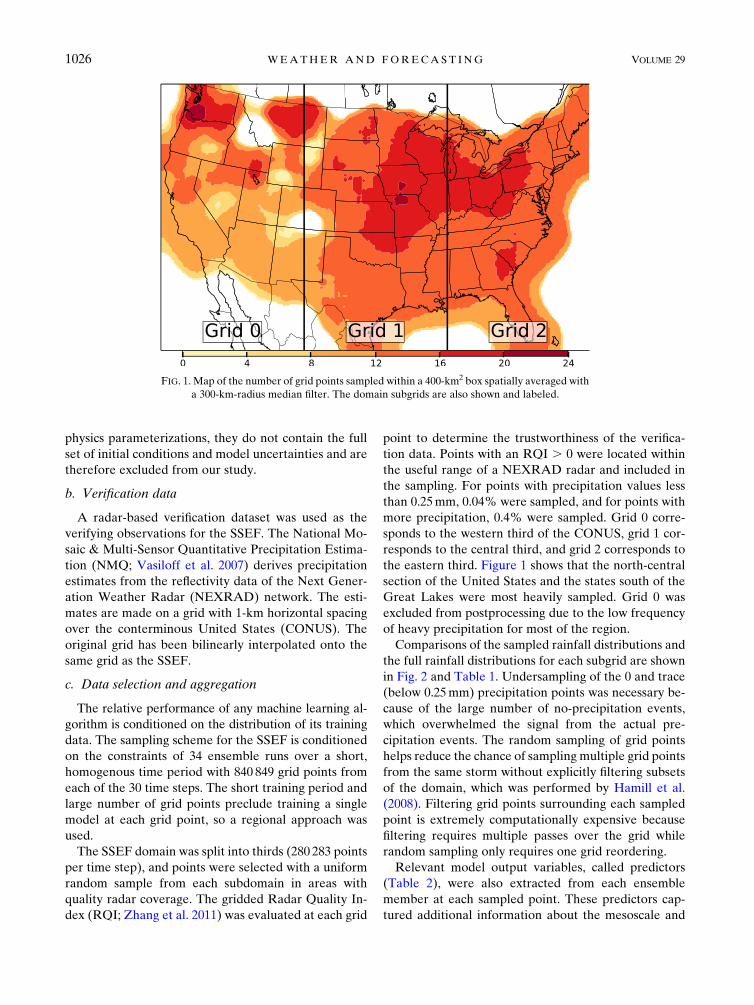
more precipitation, 0.4% were sampled. Grid 0 corre-

sponds to the western third of the CONUS, grid 1 cor-

responds to the central third, and grid 2 corresponds to

the eastern third. Figure 1 shows that the north-central

section of the United States and the states south of the

Great Lakes were most heavily sampled. Grid 0 was

excluded from postprocessing due to the low frequency

of heavy precipitation for most of the region.

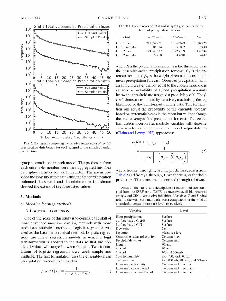
Comparisons of the sampled rainfall distributions and

the full rainfall distributions for each subgrid are shown

in Fig. 2 and Table 1. Undersampling of the 0 and trace

(below 0.25mm) precipitation points was necessary be-

cause of the large number of no-precipitation events,

which overwhelmed the signal from the actual pre-

cipitation events. The random sampling of grid points

helps reduce the chance of sampling multiple grid points

from the same storm without explicitly filtering subsets

of the domain, which was performed by Hamill et al.

(2008). Filtering grid points surrounding each sampled

point is extremely computationally expensive because

filtering requires multiple passes over the grid while

random sampling only requires one grid reordering.

Relevant model output variables, called predictors

(Table 2), were also extracted from each ensemble

member at each sampled point. These predictors cap-

tured additional information about the mesoscale and

FIG. 1. Map of the number of grid points sampled within a 400-km2 box spatially averaged with

a 300-km-radius median filter. The domain subgrids are also shown and labeled.

1026 WEATHER AND FORECAST ING VOLUME 29

synoptic conditions in each model. The predictors from

each ensemble member were then aggregated into four

descriptive statistics for each predictor. The mean pro-

vided themost likely forecast value, the standard deviation

estimated the spread, and the minimum and maximum

showed the extent of the forecasted values.

3. Methods

a. Machine learning methods

1) LOGISTIC REGRESSION

One of the goals of this study is to compare the skill of

more advanced machine learning methods with more

traditional statistical methods. Logistic regression was

used as the baseline statistical method. Logistic regres-

sions are linear regression models in which a logit

transformation is applied to the data so that the pre-

dicted values will range between 0 and 1. Two formu-

lations of logistic regression were used: simple and

multiple. The first formulation uses the ensemble-mean

precipitation forecast expressed as

p(R$ t j x1)51

11 e2(b01b

1x1), (1)

whereR is the precipitation amount, t is the threshold, x1 is

the ensemble-mean precipitation forecast, b0 is the in-

tercept term, and b1 is the weight given to the ensemble-

mean precipitation forecast. Observed precipitation with

an amount greater than or equal to the chosen threshold is

assigned a probability of 1, and precipitation amounts

below the threshold are assigned a probability of 0. The b

coefficients are estimated by iterativelymaximizing the log

likelihood of the transformed training data. This formula-

tion will adjust the probability of the ensemble forecast

based on systematic biases in the mean but will not change

the areal coverage of the precipitation forecasts. The second

formulation incorporates multiple variables with stepwise

variable selection similar to standardmodel output statistics

(Glahn and Lowry 1972) approaches:

p(R$ t j x1, x2, . . . , xn)

51

11 exp

"2

b01 �

N

n51

bnxn

!# , (2)

where from x1 through xn are the predictors chosen from

Table 2 and from b1 through bn are the weights for those

predictors. The terms are determined through a forward

TABLE 1. Frequencies of total and sampled grid points for the

different precipitation thresholds.

Grid 0–0.25mm 0.25–6mm 6mm

Grid 1 total 218 052 271 13 062 623 1 884 725

Grid 1 sampled 86 704 51 802 7490

Grid 2 total 194 343 572 10 923 189 1 137 694

Grid 2 sampled 77 210 43 218 4497

TABLE 2. The names and descriptions of model predictors sam-

pled from the SSEF runs. CAPE is convective available potential

energy, and CIN is convective inhibition. Variables U and V wind

refer to the west–east and south–north components of the wind at

a particular constant-pressure level, respectively.

Variable Level

Hour precipitation Surface

Surface-based CAPE Surface

Surface-based CIN Surface

Dewpoint 2m

Pressure Mean sea level

Composite radar reflectivity Column max

Precipitable water Column sum

Height 700mb

U wind 700mb

V wind 700 and 500mb

Specific humidity 850, 700, and 500mb

Temperature 2m, 850mb, 700mb, and 500mb

Hour max reflectivity Column and time max

Hour max upward wind Column and time max

Hour max downward wind Column and time max

FIG. 2. Histogram comparing the relative frequencies of the full

precipitation distribution for each subgrid to the sampled rainfall

distributions.

AUGUST 2014 GAGNE ET AL . 1027

selection process that finds the set of up to 15 terms that

minimize the Akaike information criterion (Akaike

1974), which rewards goodness of fit but penalizes for

large numbers of terms. This approach does produce the

best-fit regressionmodel given the available parameters,

but the searching process can take extensive time given

the large dimensionality of the training set. The gener-

alized linear model (glm) and stepwise variable selec-

tion (step) functions in theR statistical package are used

to generate the logistic regressions. A more detailed

description of logistic regression and the fitting process

can be found in James et al. (2013).

2) RANDOM FOREST

A nonparametric, nonlinear alternative to linear re-

gression is the classification and regression decision tree

(Breiman 1984). Decision trees recursively partition a

multidimensional dataset into successively smaller sub-

domains by selecting variables and decision thresholds

that maximize a dissimilarity metric. At each node in the

tree, every predictor is evaluated with the dissimilarity

metric, and the predictor and threshold with the highest

metric value are selected as the splitting criteria for that

node. After enough partitions, each subdomain is simi-

lar enough that the prediction can be approximated with

a single value. The primary advantages of decision trees

are that they can be human readable and perform vari-

able selection as part of the model growing process. The

disadvantages lie in the brittleness of the trees. Trees can

undergo significant structural shifts due to small varia-

tions in the training dataset, which results in large error

variance.

Random forests (Breiman 2001) consist of an en-

semble of classification and regression trees (Breiman

1984) with two key modifications. First, the training data

cases are bootstrap resampled with replacement for

each tree in the ensemble. Second, a random subset of

the predictors is selected for evaluation at each node.

The final prediction from the forest is the mean of the

predicted probabilities from each tree. Random forests

can produce both probabilistic and regression predictions

through thismethod. The random forest method contains

a few advantages that often lead to performance increases

over traditional regression methods. The averaging of the

results from multiple trees produces a smoother range of

values than individual decision trees while also reducing

the sensitivity of the model predictions to minor differ-

ences in the training set (Strobl et al. 2008). The random

selection of predictors within the tree-building process

allows for less optimal predictors to be included in the

model and increases the likelihood of the discovery of

interaction effects among predictors that would be

missed by the stepwise selection method used in logistic

regression (Strobl et al. 2008). Random forests have

been shown to improve predictive performance on mul-

tiple problem domains in meteorology, including storm

classification (Gagne et al. 2009), aviation turbulence

(Williams 2013), and wind energy forecasting (Kusiak

and Verma 2011). For this project, we used the R ran-

domForest library, which implements the original ap-

proach (Breiman 2001). For the parameter settings, we

chose to use 100 trees, aminimumnode size of 20, and the

default values for all other parameters. A more detailed

description of the random forest method can be found in

James et al. (2013).

In addition to gains in performance, the random forest

methodology can also be used to rank the importance of

each input variable (Breiman 2001). Variable impor-

tance is computed by first calculating the accuracy of

each tree in the forest on classifying the cases that were

not selected for training, known as the out-of-bag cases.

Within the out-of-bag cases, the values of each variable

are randomly rearranged, or permuted, and those cases

are then reevaluated by each tree. The mean variable

importance score is then the difference in prediction

accuracy on the out-of-bag cases averaged over all trees.

Variable importance scores can vary randomly among

forests trained on the same dataset, so the variable im-

portance scores from each of the 34 forests trained for

cross validation were averaged together for a more ro-

bust ranking.

b. Evaluation methods

Two scores were used to assess the probabilistic

forecasts. The Brier skill score (BSS; Brier 1950) is one

method used to evaluate probabilistic forecasts. The

Brier skill score can be decomposed into three terms

(Murphy 1973):

BSS5

1

N�K

k51

nk(ok 2o)221

N�K

k51

nk(pk2 ok)2

o(12 o), (3)

where N is the number of forecasts, K is the number of

probability bins, nk is the number of forecasts in each

probability bin, ok is the observed relative frequency for

each bin, o is the climatological frequency, and pk is the

forecast probability for a particular bin k. The first term

in the numerator describes the resolution of the forecast

probability, which should bemaximized and increases as

the observed relative frequency differs more from cli-

matology. The second term in the numerator describes

the reliability of the forecast probability, which should

be minimized and decreases with smaller differences

between the forecast probability and observed relative

frequency. The denominator term is the uncertainty,

1028 WEATHER AND FORECAST ING VOLUME 29

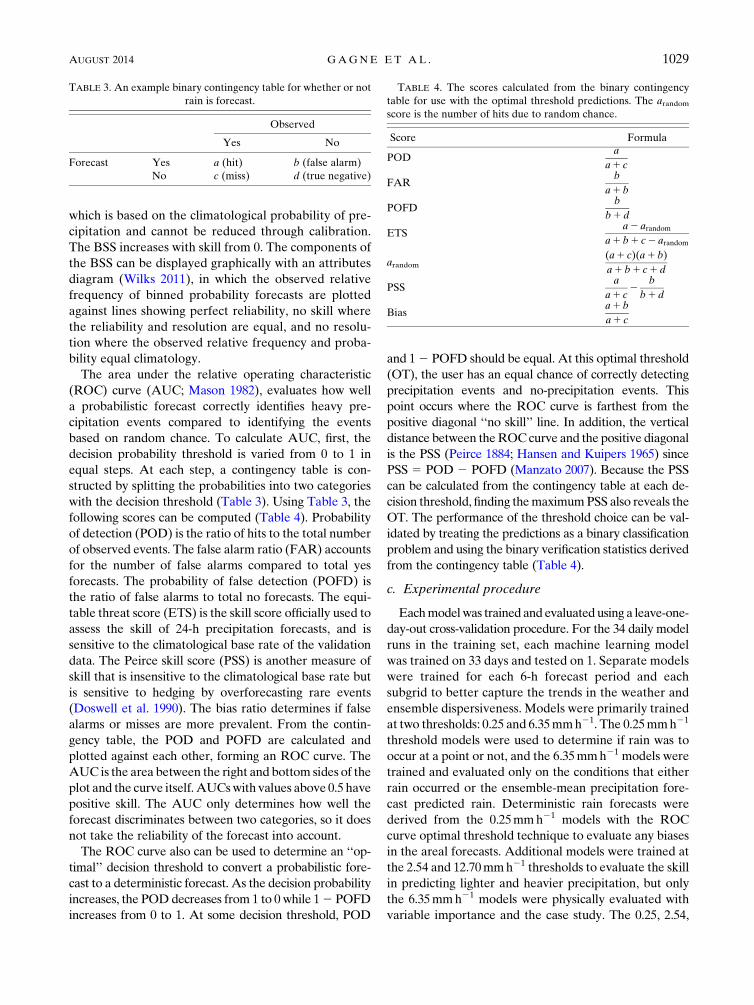
which is based on the climatological probability of pre-

cipitation and cannot be reduced through calibration.

The BSS increases with skill from 0. The components of

the BSS can be displayed graphically with an attributes

diagram (Wilks 2011), in which the observed relative

frequency of binned probability forecasts are plotted

against lines showing perfect reliability, no skill where

the reliability and resolution are equal, and no resolu-

tion where the observed relative frequency and proba-

bility equal climatology.

The area under the relative operating characteristic

(ROC) curve (AUC; Mason 1982), evaluates how well

a probabilistic forecast correctly identifies heavy pre-

cipitation events compared to identifying the events

based on random chance. To calculate AUC, first, the

decision probability threshold is varied from 0 to 1 in

equal steps. At each step, a contingency table is con-

structed by splitting the probabilities into two categories

with the decision threshold (Table 3). Using Table 3, the

following scores can be computed (Table 4). Probability

of detection (POD) is the ratio of hits to the total number

of observed events. The false alarm ratio (FAR) accounts

for the number of false alarms compared to total yes

forecasts. The probability of false detection (POFD) is

the ratio of false alarms to total no forecasts. The equi-

table threat score (ETS) is the skill score officially used to

assess the skill of 24-h precipitation forecasts, and is

sensitive to the climatological base rate of the validation

data. The Peirce skill score (PSS) is another measure of

skill that is insensitive to the climatological base rate but

is sensitive to hedging by overforecasting rare events

(Doswell et al. 1990). The bias ratio determines if false

alarms or misses are more prevalent. From the contin-

gency table, the POD and POFD are calculated and

plotted against each other, forming an ROC curve. The

AUC is the area between the right and bottom sides of the

plot and the curve itself.AUCswith values above 0.5 have

positive skill. The AUC only determines how well the

forecast discriminates between two categories, so it does

not take the reliability of the forecast into account.

The ROC curve also can be used to determine an ‘‘op-

timal’’ decision threshold to convert a probabilistic fore-

cast to a deterministic forecast. As the decision probability

increases, the PODdecreases from 1 to 0 while 12 POFD

increases from 0 to 1. At some decision threshold, POD

and 12 POFD should be equal. At this optimal threshold

(OT), the user has an equal chance of correctly detecting

precipitation events and no-precipitation events. This

point occurs where the ROC curve is farthest from the

positive diagonal ‘‘no skill’’ line. In addition, the vertical

distance between theROCcurve and the positive diagonal

is the PSS (Peirce 1884; Hansen and Kuipers 1965) since

PSS 5 POD 2 POFD (Manzato 2007). Because the PSS

can be calculated from the contingency table at each de-

cision threshold, finding themaximumPSS also reveals the

OT. The performance of the threshold choice can be val-

idated by treating the predictions as a binary classification

problem and using the binary verification statistics derived

from the contingency table (Table 4).

c. Experimental procedure

Eachmodelwas trained and evaluated using a leave-one-

day-out cross-validation procedure. For the 34 daily model

runs in the training set, each machine learning model

was trained on 33 days and tested on 1. Separate models

were trained for each 6-h forecast period and each

subgrid to better capture the trends in the weather and

ensemble dispersiveness. Models were primarily trained

at two thresholds: 0.25 and 6.35mmh21. The 0.25mmh21

threshold models were used to determine if rain was to

occur at a point or not, and the 6.35mmh21 models were

trained and evaluated only on the conditions that either

rain occurred or the ensemble-mean precipitation fore-

cast predicted rain. Deterministic rain forecasts were

derived from the 0.25mmh21 models with the ROC

curve optimal threshold technique to evaluate any biases

in the areal forecasts. Additional models were trained at

the 2.54 and 12.70mmh21 thresholds to evaluate the skill

in predicting lighter and heavier precipitation, but only

the 6.35mmh21 models were physically evaluated with

variable importance and the case study. The 0.25, 2.54,

TABLE 3. An example binary contingency table for whether or not

rain is forecast.

Observed

Yes No

Forecast Yes a (hit) b (false alarm)

No c (miss) d (true negative)

TABLE 4. The scores calculated from the binary contingency

table for use with the optimal threshold predictions. The arandomscore is the number of hits due to random chance.

Score Formula

PODa

a1 c

FARb

a1b

POFDb

b1 d

ETSa2 arandom

a1b1 c2 arandom

arandom(a1 c)(a1b)

a1b1 c1d

PSSa

a1 c2

b

b1d

Biasa1b

a1 c

AUGUST 2014 GAGNE ET AL . 1029

6.35, and 12.70mmh21 values were chosen because they

correspond to the 0.01, 0.1, 0.25, and 0.5 in. h21 thresh-

olds, respectively, that are used for determining trace and

heavy precipitation amounts. The probabilities shown in

the case study are the joint probabilities of precipitation

greater than or equal to 6.35 and 0.25mmh21. They were

calculated by multiplying the conditional probability of

precipitation greater than or equal to 6.35mmh21 with

the probability of precipitation greater than or equal to

0.25mmh21.

4. Results

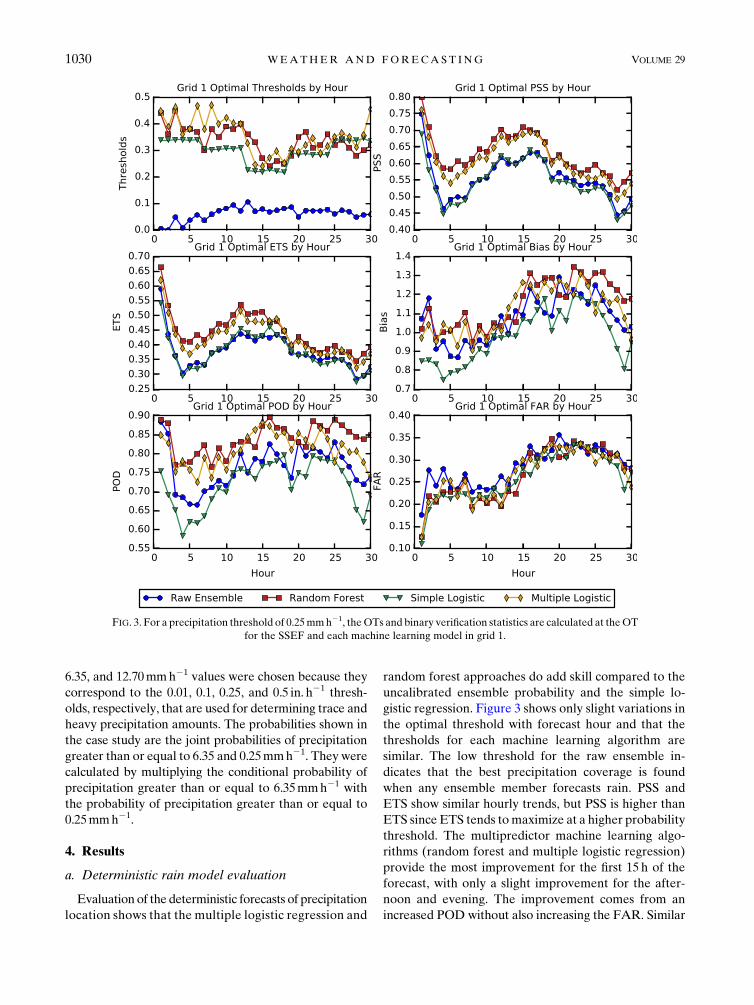
a. Deterministic rain model evaluation

Evaluation of the deterministic forecasts of precipitation

location shows that the multiple logistic regression and

random forest approaches do add skill compared to the

uncalibrated ensemble probability and the simple lo-

gistic regression. Figure 3 shows only slight variations in

the optimal threshold with forecast hour and that the

thresholds for each machine learning algorithm are

similar. The low threshold for the raw ensemble in-

dicates that the best precipitation coverage is found

when any ensemble member forecasts rain. PSS and

ETS show similar hourly trends, but PSS is higher than

ETS since ETS tends tomaximize at a higher probability

threshold. The multipredictor machine learning algo-

rithms (random forest and multiple logistic regression)

provide the most improvement for the first 15 h of the

forecast, with only a slight improvement for the after-

noon and evening. The improvement comes from an

increased POD without also increasing the FAR. Similar

FIG. 3. For a precipitation threshold of 0.25mmh21, theOTs and binary verification statistics are calculated at theOT

for the SSEF and each machine learning model in grid 1.

1030 WEATHER AND FORECAST ING VOLUME 29

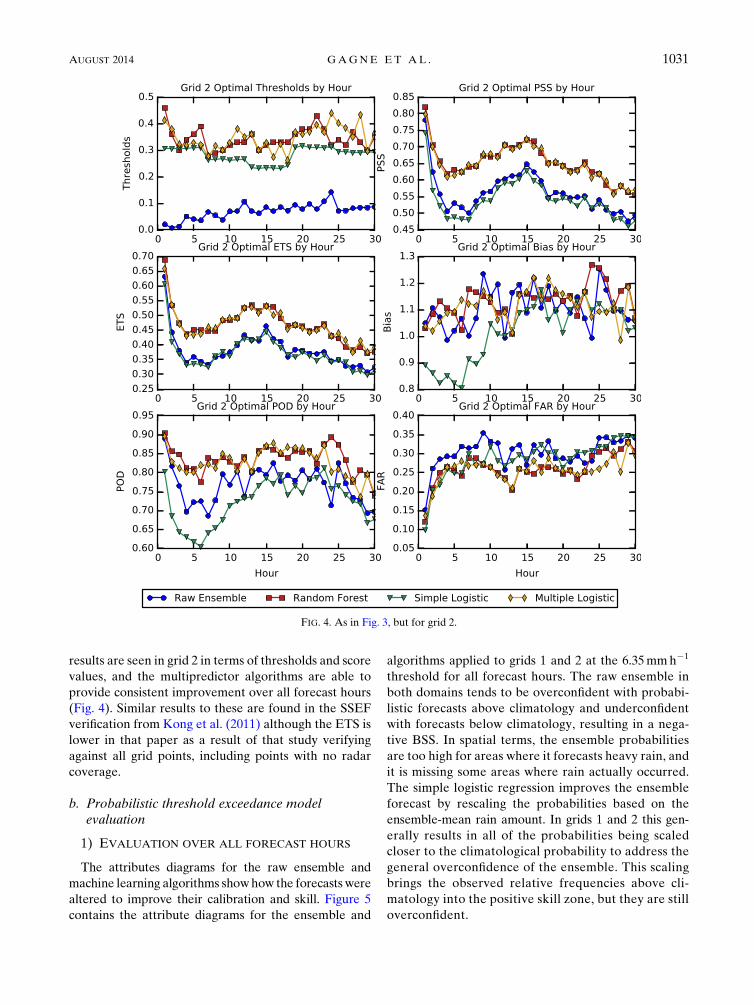
results are seen in grid 2 in terms of thresholds and score

values, and the multipredictor algorithms are able to

provide consistent improvement over all forecast hours

(Fig. 4). Similar results to these are found in the SSEF

verification from Kong et al. (2011) although the ETS is

lower in that paper as a result of that study verifying

against all grid points, including points with no radar

coverage.

b. Probabilistic threshold exceedance modelevaluation

1) EVALUATION OVER ALL FORECAST HOURS

The attributes diagrams for the raw ensemble and

machine learning algorithms showhow the forecasts were

altered to improve their calibration and skill. Figure 5

contains the attribute diagrams for the ensemble and

algorithms applied to grids 1 and 2 at the 6.35mmh21

threshold for all forecast hours. The raw ensemble in

both domains tends to be overconfident with probabi-

listic forecasts above climatology and underconfident

with forecasts below climatology, resulting in a nega-

tive BSS. In spatial terms, the ensemble probabilities

are too high for areas where it forecasts heavy rain, and

it is missing some areas where rain actually occurred.

The simple logistic regression improves the ensemble

forecast by rescaling the probabilities based on the

ensemble-mean rain amount. In grids 1 and 2 this gen-

erally results in all of the probabilities being scaled

closer to the climatological probability to address the

general overconfidence of the ensemble. This scaling

brings the observed relative frequencies above cli-

matology into the positive skill zone, but they are still

overconfident.

FIG. 4. As in Fig. 3, but for grid 2.

AUGUST 2014 GAGNE ET AL . 1031

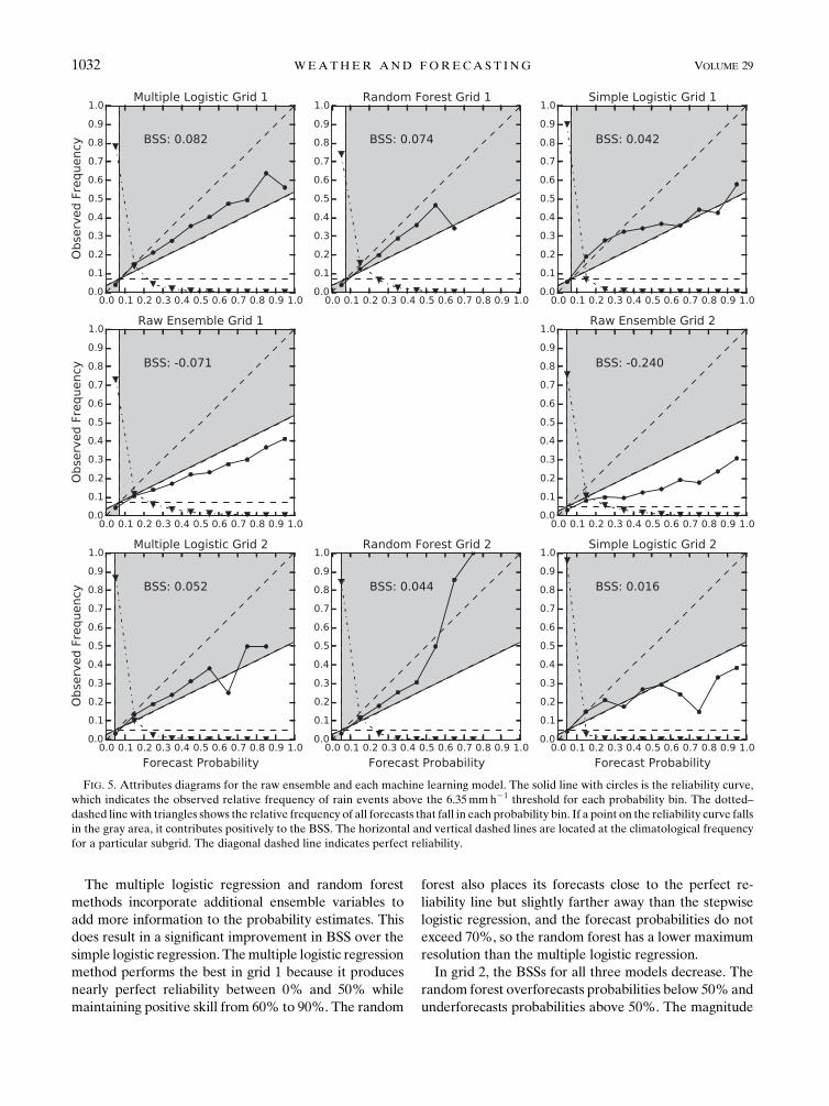
The multiple logistic regression and random forest

methods incorporate additional ensemble variables to

add more information to the probability estimates. This

does result in a significant improvement in BSS over the

simple logistic regression. Themultiple logistic regression

method performs the best in grid 1 because it produces

nearly perfect reliability between 0% and 50% while

maintaining positive skill from 60% to 90%. The random

forest also places its forecasts close to the perfect re-

liability line but slightly farther away than the stepwise

logistic regression, and the forecast probabilities do not

exceed 70%, so the random forest has a lower maximum

resolution than the multiple logistic regression.

In grid 2, the BSSs for all three models decrease. The

random forest overforecasts probabilities below 50%and

underforecasts probabilities above 50%. The magnitude

FIG. 5. Attributes diagrams for the raw ensemble and each machine learning model. The solid line with circles is the reliability curve,

which indicates the observed relative frequency of rain events above the 6.35mmh21 threshold for each probability bin. The dotted–

dashed linewith triangles shows the relative frequency of all forecasts that fall in each probability bin. If a point on the reliability curve falls

in the gray area, it contributes positively to the BSS. The horizontal and vertical dashed lines are located at the climatological frequency

for a particular subgrid. The diagonal dashed line indicates perfect reliability.

1032 WEATHER AND FORECAST ING VOLUME 29

of the underforecasting may be overestimated because of

the small number of high probability forecasts. The

multiple logistic regression method performs better with

the lower-probability forecasts but has negative skill with

the higher probabilities. This poorer performancemay be

due to having fewer heavy rain events in grid 2 during the

study time period.

The ROC curves show that the multiple-predictor

machine learning algorithms enhance the discrimination

abilities of the ensemble. The raw ensembles in both

subgrids have slightly positive skill in terms of AUC

(Fig. 6). At the optimal PSS threshold, the raw en-

semble detects only 67% of heavy rain events (POD) in

grid 1, and 86% of its positive forecasts are false alarms

(FAR). In grid 2, the detection ability is worse, with

a 66%POD and a 91%FAR. Bias scores greater than 1

indicate a larger proportion of false alarms than misses.

Since the simple logistic regression rescales the pre-

dictions over a smaller probability range, it has a

slightly lower AUC than does the raw ensemble. Its

optimal threshold is higher than the raw ensemble, so it

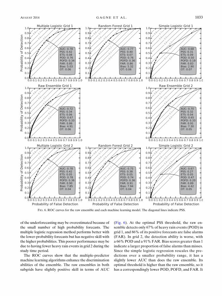
has a correspondingly lower POD, POFD, and FAR. It

FIG. 6. ROC curves for the raw ensemble and each machine learning model. The diagonal lines indicate PSS.

AUGUST 2014 GAGNE ET AL . 1033

also has a smaller bias score at the optimal threshold.

The multiple logistic regression and random forest

have a much larger AUC and POD and similar FAR

compared to the raw ensemble. The multiple logistic

regression and random forest approaches have very

similar scores with only slight differences in their

POFD, FAR, and bias. The same relationships hold in

grid 2 except that there is a slightly larger difference in

the scores of the multiple logistic regression and ran-

dom forest methods. The overall scores are also slightly

lower for grid 2, which is likely due to the lower fre-

quency of convective precipitation events in the train-

ing dataset.

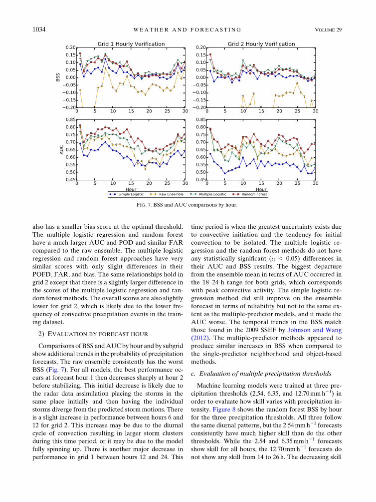
2) EVALUATION BY FORECAST HOUR

Comparisons of BSS andAUCby hour and by subgrid

show additional trends in the probability of precipitation

forecasts. The raw ensemble consistently has the worst

BSS (Fig. 7). For all models, the best performance oc-

curs at forecast hour 1 then decreases sharply at hour 2

before stabilizing. This initial decrease is likely due to

the radar data assimilation placing the storms in the

same place initially and then having the individual

storms diverge from the predicted stormmotions. There

is a slight increase in performance between hours 6 and

12 for grid 2. This increase may be due to the diurnal

cycle of convection resulting in larger storm clusters

during this time period, or it may be due to the model

fully spinning up. There is another major decrease in

performance in grid 1 between hours 12 and 24. This

time period is when the greatest uncertainty exists due

to convective initiation and the tendency for initial

convection to be isolated. The multiple logistic re-

gression and the random forest methods do not have

any statistically significant (a , 0.05) differences in

their AUC and BSS results. The biggest departure

from the ensemble mean in terms of AUC occurred in

the 18–24-h range for both grids, which corresponds

with peak convective activity. The simple logistic re-

gression method did still improve on the ensemble

forecast in terms of reliability but not to the same ex-

tent as the multiple-predictor models, and it made the

AUC worse. The temporal trends in the BSS match

those found in the 2009 SSEF by Johnson and Wang

(2012). The multiple-predictor methods appeared to

produce similar increases in BSS when compared to

the single-predictor neighborhood and object-based

methods.

c. Evaluation of multiple precipitation thresholds

Machine learning models were trained at three pre-

cipitation thresholds (2.54, 6.35, and 12.70mmh21) in

order to evaluate how skill varies with precipitation in-

tensity. Figure 8 shows the random forest BSS by hour

for the three precipitation thresholds. All three follow

the same diurnal patterns, but the 2.54mmh21 forecasts

consistently have much higher skill than do the other

thresholds. While the 2.54 and 6.35mmh21 forecasts

show skill for all hours, the 12.70mmh21 forecasts do

not show any skill from 14 to 26 h. The decreasing skill

FIG. 7. BSS and AUC comparisons by hour.

1034 WEATHER AND FORECAST ING VOLUME 29

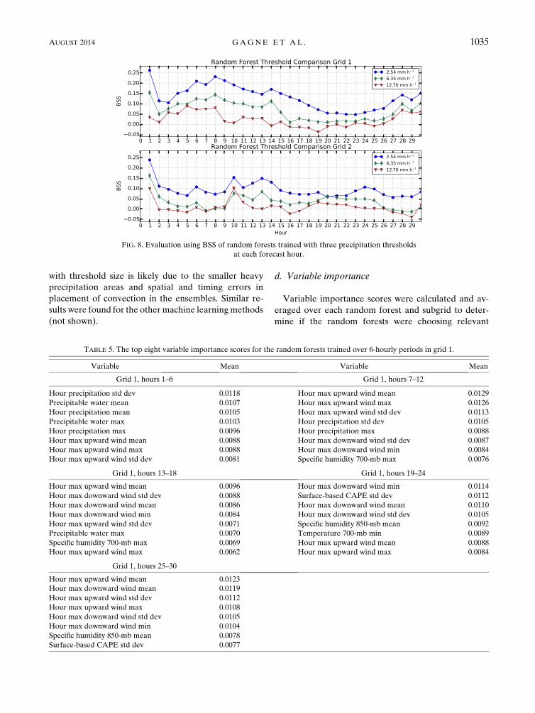
with threshold size is likely due to the smaller heavy

precipitation areas and spatial and timing errors in

placement of convection in the ensembles. Similar re-

sults were found for the other machine learningmethods

(not shown).

d. Variable importance

Variable importance scores were calculated and av-

eraged over each random forest and subgrid to deter-

mine if the random forests were choosing relevant

TABLE 5. The top eight variable importance scores for the random forests trained over 6-hourly periods in grid 1.

Variable Mean Variable Mean

Grid 1, hours 1–6 Grid 1, hours 7–12

Hour precipitation std dev 0.0118 Hour max upward wind mean 0.0129

Precipitable water mean 0.0107 Hour max upward wind max 0.0126

Hour precipitation mean 0.0105 Hour max upward wind std dev 0.0113

Precipitable water max 0.0103 Hour precipitation std dev 0.0105

Hour precipitation max 0.0096 Hour precipitation max 0.0088

Hour max upward wind mean 0.0088 Hour max downward wind std dev 0.0087

Hour max upward wind max 0.0088 Hour max downward wind min 0.0084

Hour max upward wind std dev 0.0081 Specific humidity 700-mb max 0.0076

Grid 1, hours 13–18 Grid 1, hours 19–24

Hour max upward wind mean 0.0096 Hour max downward wind min 0.0114

Hour max downward wind std dev 0.0088 Surface-based CAPE std dev 0.0112

Hour max downward wind mean 0.0086 Hour max downward wind mean 0.0110

Hour max downward wind min 0.0084 Hour max downward wind std dev 0.0105

Hour max upward wind std dev 0.0071 Specific humidity 850-mb mean 0.0092

Precipitable water max 0.0070 Temperature 700-mb min 0.0089

Specific humidity 700-mb max 0.0069 Hour max upward wind mean 0.0088

Hour max upward wind max 0.0062 Hour max upward wind max 0.0084

Grid 1, hours 25–30

Hour max upward wind mean 0.0123

Hour max downward wind mean 0.0119

Hour max upward wind std dev 0.0112

Hour max upward wind max 0.0108

Hour max downward wind std dev 0.0105

Hour max downward wind min 0.0104

Specific humidity 850-mb mean 0.0078

Surface-based CAPE std dev 0.0077

FIG. 8. Evaluation using BSS of random forests trained with three precipitation thresholds

at each forecast hour.

AUGUST 2014 GAGNE ET AL . 1035

variables and how the choice of variables was affected

by region. Variable importance is indicative of how

randomizing the value of each variable affects the ran-

dom forest performance. This process accounts for how

often a variable is used in the model, the depth of the

variable in the tree, and the number of cases that transit

through the branch containing that variable, but the

importance score cannot be decomposed into those

factors. The top eight variable importance scores for the

random forests trained on each 6-h period in grid 1 are

shown in Table 5. In the first 6 h, all of the top five vari-

ables are aggregations of the hour precipitation or pre-

cipitable water, with the rest being hourmaximum upward

wind. In this time period, the ensemble members are very

similar, so there is great overlap among the precipitation

regions. By hours 7–12, the maximum upward wind be-

comes more dominant in the rankings, although the pre-

cipitation maximum and standard deviation are still found

among the top five variables. Vertical velocities become

the most common feature in hours 13–18 with only pre-

cipitablewater and specific humidity contributingmoisture

information. For hours 19–30, the standard deviation of

surface-based CAPE appears, which is likely associated

with the presence of nearby boundaries.

The grid 2 variable importance scores (Table 6) high-

light the greater importance of moisture and lower im-

portance of vertical velocities in the eastern United States.

The predicted precipitation is again only important in

hours 1–12, but the precipitable water and specific hu-

midity show high importance through the entire forecast

period. Upward and downward winds are in the rankings

for each time period, but they tend to be toward the bot-

tom of the top eight. Surface-based CAPE is also impor-

tant in the later hours of the forecasts, but the mean and

maximum are selected instead of the standard deviation.

e. Case study: 13 May 2010

The case of 13 May 2010 illustrates the spatial charac-

teristics, strengths, and weaknesses of the precipitation

forecasts from the SSEF and the machine learning

methods. Since SSEF is run through forecast hour 30,

the last six forecast hours of one run overlap with the

first six hours of the next run. This overlap allows for the

comparison of two runs on the same observations and

illustrates the effects of lead time on the forecast prob-

abilities. Figure 9 shows the distribution of the observed

1-h precipitation at 0200 UTC 13 May. The bulk of the

precipitation originates from a broken line of discrete

TABLE 6. The top eight variable importance scores for the random forests trained over 6-hourly periods in grid 2.

Variable Mean Variable Mean

Grid 2, hours 1–6 Grid 2, hours 7–12

Hour precipitation mean 0.0116 Precipitable water mean 0.0111

Precipitable water mean 0.0114 Precipitable water min 0.0085

Precipitable water min 0.0104 Precipitable water max 0.0079

Precipitable water max 0.0097 Hour max upward wind mean 0.0077

Hour max upward wind mean 0.0094 Hour max upward wind std dev 0.0066

Hour max reflectivity mean 0.0091 Hour precipitation mean 0.0065

Hour max upward wind max 0.0082 Hour precipitation std dev 0.0062

Hour precipitation max 0.0080 Hour max upward wind max 0.0062

Grid 2, hours 13–18 Grid 2, hours 19–24

Precipitable water mean 0.0077 Specific humidity 850-mb mean 0.0162

Hour max upward wind mean 0.0075 Specific humidity 850-mb max 0.0128

Specific humidity 850-mb mean 0.0065 Hour max upward wind mean 0.0110

Precipitable water min 0.0065 Surface-based CAPE max 0.0106

Precipitable water max 0.0056 Surface-based CAPE mean 0.0103

Temperature 700-mb mean 0.0056 Hour max upward wind std dev 0.0101

Hour max upward wind max 0.0055 Hour max downward wind mean 0.0098

Temperature 500-mb min 0.0054 Hour max upward wind max 0.0090

Grid 2, hours 25–30

Specific humidity 850-mb mean 0.0114

Hour max upward wind mean 0.0094

Precipitable water mean 0.0084

Specific humidity 850-mb max 0.0083

Hour precipitation std dev 0.0072

Hour max upward wind max 0.0071

Hour max downward wind mean 0.0070

Surface-based CAPE max 0.0069

1036 WEATHER AND FORECAST ING VOLUME 29

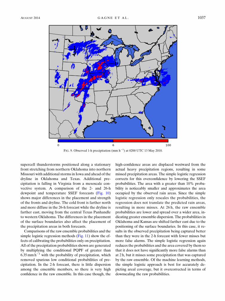
supercell thunderstorms positioned along a stationary

front stretching from northern Oklahoma into northern

Missouri with additional storms in Iowa and ahead of the

dryline in Oklahoma and Texas. Additional pre-

cipitation is falling in Virginia from a mesoscale con-

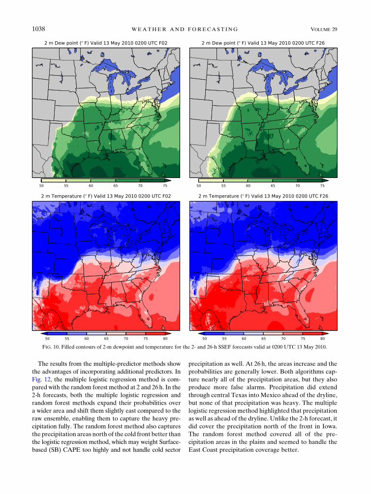
vective system. A comparison of the 2- and 26-h

dewpoint and temperature SSEF forecasts (Fig. 10)

shows major differences in the placement and strength

of the fronts and dryline. The cold front is farther north

and more diffuse in the 26-h forecast while the dryline is

farther east, moving from the central Texas Panhandle

to western Oklahoma. The differences in the placement

of the surface boundaries also affect the placement of

the precipitation areas in both forecasts.

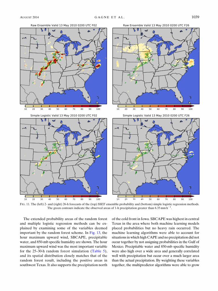
Comparisons of the raw ensemble probabilities and the

simple logistic regression methods (Fig. 11) show the ef-

fects of calibrating the probabilities only on precipitation.

All of the precipitation probabilities shown are generated

by multiplying the conditional PQPF of greater than

6.35mmh21 with the probability of precipitation, which

removed spurious low conditional probabilities of pre-

cipitation. In the 2-h forecast, there is little dispersion

among the ensemble members, so there is very high

confidence in the raw ensemble. In this case though, the

high-confidence areas are displaced westward from the

actual heavy precipitation regions, resulting in some

missed precipitation areas. The simple logistic regression

corrects for this overconfidence by lowering the SSEF

probabilities. The area with a greater than 10% proba-

bility is noticeably smaller and approximates the area

occupied by the observed rain areas. Since the simple

logistic regression only rescales the probabilities, the

regression does not translate the predicted rain areas,

resulting in more misses. At 26 h, the raw ensemble

probabilities are lower and spread over a wider area, in-

dicating greater ensemble dispersion. The probabilities in

Oklahoma and Kansas are shifted farther east due to the

positioning of the surface boundaries. In this case, it re-

sults in the observed precipitation being captured better

than they were in the 2-h forecast with fewer misses but

more false alarms. The simple logistic regression again

reduces the probabilities and the area covered by them so

that it does not have significantly more false alarms than

at 2 h, but it misses some precipitation that was captured

by the raw ensemble. Of the machine learning methods,

the simple logistic approach is best for accurately de-

picting areal coverage, but it overcorrected in terms of

downscaling the raw probabilities.

FIG. 9. Observed 1-h precipitation (mm h21) at 0200 UTC 13 May 2010.

AUGUST 2014 GAGNE ET AL . 1037

The results from the multiple-predictor methods show

the advantages of incorporating additional predictors. In

Fig. 12, the multiple logistic regression method is com-

pared with the random forest method at 2 and 26h. In the

2-h forecasts, both the multiple logistic regression and

random forest methods expand their probabilities over

a wider area and shift them slightly east compared to the

raw ensemble, enabling them to capture the heavy pre-

cipitation fully. The random forest method also captures

the precipitation areas north of the cold front better than

the logistic regression method, which may weight Surface-

based (SB) CAPE too highly and not handle cold sector

precipitation as well. At 26 h, the areas increase and the

probabilities are generally lower. Both algorithms cap-

ture nearly all of the precipitation areas, but they also

produce more false alarms. Precipitation did extend

through central Texas into Mexico ahead of the dryline,

but none of that precipitation was heavy. The multiple

logistic regression method highlighted that precipitation

as well as ahead of the dryline. Unlike the 2-h forecast, it

did cover the precipitation north of the front in Iowa.

The random forest method covered all of the pre-

cipitation areas in the plains and seemed to handle the

East Coast precipitation coverage better.

FIG. 10. Filled contours of 2-m dewpoint and temperature for the 2- and 26-h SSEF forecasts valid at 0200 UTC 13 May 2010.

1038 WEATHER AND FORECAST ING VOLUME 29

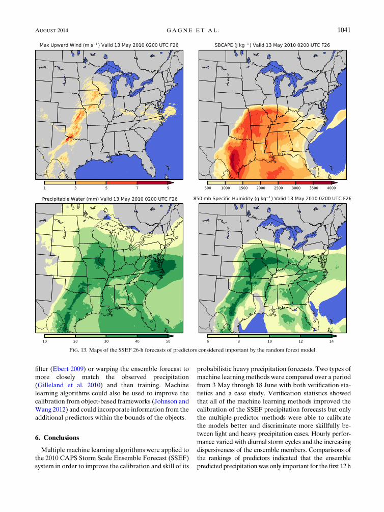
The extended probability areas of the random forest

and multiple logistic regression methods can be ex-

plained by examining some of the variables deemed

important by the random forest scheme. In Fig. 13, the

hour maximum upward wind, SBCAPE, precipitable

water, and 850-mb specific humidity are shown. The hour

maximum upward wind was the most important variable

for the 25–30-h random forest simulation (Table 5),

and its spatial distribution closely matches that of the

random forest result, including the positive areas in

southwest Texas. It also supports the precipitation north

of the cold front in Iowa. SBCAPEwas highest in central

Texas in the area where both machine learning models

placed probabilities but no heavy rain occurred. The

machine learning algorithms were able to account for

situations inwhichhighCAPEandnoprecipitationdid not

occur together by not assigning probabilities in the Gulf of

Mexico. Precipitable water and 850-mb specific humidity

were also high over a wide area and generally correlated

well with precipitation but occur over a much larger area

than the actual precipitation. By weighting these variables

together, the multipredictor algorithms were able to grow

FIG. 11. The (left) 2- and (right) 26-h forecasts of the (top) SSEF ensemble probability and (bottom) simple logistic regression methods.

The green contours indicate the observed areas of 1-h precipitation greater than 6.35mmh21.

AUGUST 2014 GAGNE ET AL . 1039

the forecasted area to include points at which the mix of

ingredients was favorable for precipitation.

5. Discussion

The results of the machine learning postprocessing of

storm-scale ensemble precipitation forecasts displayed

not only improvements to the forecasts but also some of

the limitations of the ensemble, the algorithms, and the

gridpoint-based framework. First, the postprocessing

model performance is constrained by the information

available from the ensemble. If most of the ensemble

members are predicting precipitation in the wrong place

or not at all, and the environmental conditions are also

displaced, then the machine learning algorithm will not

be able to provide much additional skill. Second, the

machine learning model will only make predictions

based on the range of cases it has previously seen. For

higher rain thresholds, the algorithms will need more

independent samples in order to make skilled pre-

dictions.Third, the gridpoint framework does not fully

account for the spatial information and error in the en-

semble. The spatial error could be incorporated further

by smoothing the verification grid with a neighborhood

FIG. 12. As in Fig. 11, but for (top) multiple logistic regression and (bottom) random forest methods.

1040 WEATHER AND FORECAST ING VOLUME 29

filter (Ebert 2009) or warping the ensemble forecast to

more closely match the observed precipitation

(Gilleland et al. 2010) and then training. Machine

learning algorithms could also be used to improve the

calibration from object-based frameworks (Johnson and

Wang 2012) and could incorporate information from the

additional predictors within the bounds of the objects.

6. Conclusions

Multiple machine learning algorithms were applied to

the 2010 CAPS Storm Scale Ensemble Forecast (SSEF)

system in order to improve the calibration and skill of its

probabilistic heavy precipitation forecasts. Two types of

machine learning methods were compared over a period

from 3 May through 18 June with both verification sta-

tistics and a case study. Verification statistics showed

that all of the machine learning methods improved the

calibration of the SSEF precipitation forecasts but only

the multiple-predictor methods were able to calibrate

the models better and discriminate more skillfully be-

tween light and heavy precipitation cases. Hourly perfor-

mance varied with diurnal storm cycles and the increasing

dispersiveness of the ensemble members. Comparisons of

the rankings of predictors indicated that the ensemble

predicted precipitationwas only important for the first 12h

FIG. 13. Maps of the SSEF 26-h forecasts of predictors considered important by the random forest model.

AUGUST 2014 GAGNE ET AL . 1041

of the model runs. After that period, the upward wind and

atmospheric moisture variables became better indicators

of the placement of precipitation. The case study showed

that the multiple-predictor machine learning methods

could shift the probability maxima to better match the

actual precipitation areas, but they would also produce

more false alarm areas in the process. For shorter-term

forecasts, the false corrections were made without a sig-

nificant increase in the false alarm area. Calibrating the

probabilities with only ensemble rainfall predictions re-

sults in predicted areas that are too small and still displaced

from the observed precipitation. The multiple-predictor

machine learning algorithms did prove especially benefi-

cial in that situation. Ultimately, machine learning tech-

niques can provide an enhancement to precipitation

forecasts by consistently maximizing the potential of the

available information.

Acknowledgments. Special thanks go to DJGII’s mas-

ter’s committee members: Fanyou Kong and Michael

Richman. Zac Flamig provided assistance with the NMQ

data. CAPS SSEF forecasts were supported by a grant

(NWSPO-2010-201696) from the NOAA Collaborative

Science, Technology, and Applied Research (CSTAR)

Program and the forecasts were produced at the National

Institute for Computational Science (http://www.nics.

tennessee.edu/). Scientists at CAPS, including Fanyou

Kong, Kevin Thomas, Yunheng Wang, and Keith

Brewster contributed to the design and production of the

CAPS ensemble forecasts. This study was funded by the

NSF Graduate Research Fellowship under Grant

2011099434 and byNSFGrantAGS-0802888. The editor,

Michael Baldwin, and the two anonymous reviewers

provided very helpful feedback that strengthened the

quality of the paper.

REFERENCES

Akaike, H., 1974: A new look at the statistical model identifica-

tion. IEEE Trans. Autom. Control, 19, 716–723, doi:10.1109/

TAC.1974.1100705.

Applequist, S., G. E. Gahrs, R. L. Pfeffer, and X. Niu, 2002:

Comparison of methodologies for probabilistic quantitative

precipitation forecasting. Wea. Forecasting, 17, 783–799,

doi:10.1175/1520-0434(2002)017,0783:COMFPQ.2.0.CO;2.

Ashley, S. T., andW. S. Ashley, 2008: Flood fatalities in the United

States. J. Appl. Meteor. Climatol., 47, 805–818, doi:10.1175/

2007JAMC1611.1.

Breiman, L., 1984: Classification and Regression Trees.Wadsworth

International Group, 358 pp.

——, 2001: Random forests. Mach. Learn., 45, 5–32, doi:10.1023/

A:1010933404324.

Bremnes, J. B., 2004: Probabilistic forecasts of precipitation in

terms of quantiles using NWP model output. Mon. Wea.

Rev., 132, 338–347, doi:10.1175/1520-0493(2004)132,0338:

PFOPIT.2.0.CO;2.

Brier, G. W., 1950: Verification of forecasts expressed in terms

of probability. Mon. Wea. Rev., 78, 1–3, doi:10.1175/

1520-0493(1950)078,0001:VOFEIT.2.0.CO;2.

Clark, A. J., W. A. Gallus Jr., M. Xue, and F. Kong, 2009: A com-

parison of precipitation forecast skill between small convection-

allowing and large convection-parameterizing ensembles.Wea.

Forecasting, 24, 1121–1140, doi:10.1175/2009WAF2222222.1.

——, and Coauthors, 2011: Probabilistic precipitation forecast skill

as a function of ensemble size and spatial scale in a convection-

allowing ensemble.Mon.Wea. Rev., 139, 1410–1418, doi:10.1175/

2010MWR3624.1.

——, and Coauthors, 2012: An overview of the 2010 Hazardous

Weather Testbed Experimental Forecast Program Spring

Experiment. Bull. Amer. Meteor. Soc., 93, 55–74, doi:10.1175/

BAMS-D-11-00040.1.

Doswell, C. A., III, R. Davies-Jones, and D. L. Keller, 1990: On

summary measures of skill in rare event forecasting based on

contingency tables. Wea. Forecasting, 5, 576–585, doi:10.1175/

1520-0434(1990)005,0576:OSMOSI.2.0.CO;2.

——,H. E. Brooks, andR.A.Maddox, 1996: Flash flood forecasting:

An ingredients-based methodology. Wea. Forecasting, 11, 560–

581, doi:10.1175/1520-0434(1996)011,0560:FFFAIB.2.0.CO;2.

Du, J., J. McQueen, G. DiMego, Z. Toth, D. Jovic, B. Zhou, and

H. Chuang, 2006: New dimension of NCEP Short-Range En-

semble Forecasting (SREF) system: Inclusion of WRF mem-

bers. Preprints, WMO Expert Team Meeting on Ensemble

Prediction System, Exeter, United Kingdom, WMO. [Avail-

able online at http://www.emc.ncep.noaa.gov/mmb/SREF/

reference.html.]

Ebert, E. E., 2001: Ability of a poor man’s ensemble to predict

the probability and distribution of precipitation. Mon. Wea.

Rev., 129, 2461–2480, doi:10.1175/1520-0493(2001)129,2461:

AOAPMS.2.0.CO;2.

——, 2009: Neighborhood verification: A strategy for rewarding

close forecasts. Wea. Forecasting, 24, 1498–1510, doi:10.1175/

2009WAF2222251.1.

Eckel, F. A., and M. K. Walters, 1998: Calibrated probabilistic

quantitative precipitation forecasts based on the MRF

ensemble. Wea. Forecasting, 13, 1132–1147, doi:10.1175/

1520-0434(1998)013,1132:CPQPFB.2.0.CO;2.

Gagne, D. J., II, A. McGovern, and J. Brotzge, 2009: Classification

of convective areas using decision trees. J. Atmos. Oceanic

Technol., 26, 1341–1353, doi:10.1175/2008JTECHA1205.1.

——, ——, and M. Xue, 2012: Machine learning enhancement of

storm scale ensemble precipitation forecasts. Proc. Conf. on

Intelligent Data Understanding,Boulder, CO, IEEE-CIS, 39–46.

Gilleland, E., and Coauthors, 2010: Spatial forecast verification:

Image warping. NCAR Tech. Rep. NCAR/TN-4821STR, 23

pp. [Available online at http://nldr.library.ucar.edu/repository/

assets/technotes/TECH-NOTE-000-000-000-850.pdf.]

Glahn, H. R., and D. A. Lowry, 1972: The use of model output

statistics (MOS) in objective weather forecasts. J. Appl. Me-

teor., 11, 1203–1211, doi:10.1175/1520-0450(1972)011,1203:

TUOMOS.2.0.CO;2.

Hall, T., H. E. Brooks, and C. A. Doswell III, 1999: Precip-

itation forecasting using a neural network. Wea. Fore-

casting, 14, 338–345, doi:10.1175/1520-0434(1999)014,0338:

PFUANN.2.0.CO;2.

Hamill, T.M., and S. J.Colucci, 1997:Verification ofEta–RSMshort-

range ensemble forecasts. Mon. Wea. Rev., 125, 1312–1327,

doi:10.1175/1520-0493(1997)125,1312:VOERSR.2.0.CO;2.

1042 WEATHER AND FORECAST ING VOLUME 29

——, and ——, 1998: Evaluation of Eta–RSM ensemble probabi-

listic precipitation forecasts. Mon. Wea. Rev., 126, 711–724,

doi:10.1175/1520-0493(1998)126,0711:EOEREP.2.0.CO;2.

——, J. S. Whitaker, and X. Wei, 2004: Ensemble reforecasting:

Improving medium-range forecast skill using retrospective

forecasts. Mon. Wea. Rev., 132, 1434–1447, doi:10.1175/

1520-0493(2004)132,1434:ERIMFS.2.0.CO;2.

——, R. Hagedorn, and J. S. Whitaker, 2008: Probabilistic forecast

calibration using ECMWF and GFS ensemble reforecasts. Part

II: Precipitation. Mon. Wea. Rev., 136, 2620–2632, doi:10.1175/

2007MWR2411.1.

Hansen, A. W., and W. J. A. Kuipers, 1965: On the relationship

between the frequency of rain and various meteorological

parameters. Meded. Verh., 81, 2–15.

James, G., D. Witten, T. Hastie, and R. Tibshirani, 2013: An

Introduction to Statistical Learning with Applications in

R. Springer, 430 pp.

Johnson, A., and X. Wang, 2012: Verification and calibration of

neighborhood and object-based probabilistic precipitation fore-

casts from a multimodel convection-allowing ensemble. Mon.

Wea. Rev., 140, 3054–3077, doi:10.1175/MWR-D-11-00356.1.

Koizumi, K., 1999: An objective method tomodify numerical model

forecasts with newly given weather data using an artificial

neural network. Wea. Forecasting, 14, 109–118, doi:10.1175/

1520-0434(1999)014,0109:AOMTMN.2.0.CO;2.

Kong, F., and Coauthors, 2011: Evaluation of CAPS multi-model

storm-scale ensemble forecast for the NOAA HWT 2010

spring experiment. 25th Conf. on Severe Local Storms, Seattle,

WA, Amer. Meteor. Soc., P4.18. [Available online at https://

ams.confex.com/ams/25SLS/techprogram/paper_175822.htm.]

Krishnamurti, T. N., C. M. Kishtawal, T. E. LaRow, D. R.

Bachiochi, Z. Zhang, C. E. Williford, S. Gadgil, and

S. Surendran, 1999: Improved weather and seasonal climate

forecasts from multimodel superensemble. Science, 285,1548–1550, doi:10.1126/science.285.5433.1548.

Kusiak, A., and A. Verma, 2011: Prediction of status patterns of

wind turbines: A data-mining approach. J. Sol. Energy Eng.,

133, 011008, doi:10.1115/1.4003188.

Manzato, A., 2007: A note on themaximumPeirce skill score.Wea.

Forecasting, 22, 1148–1154, doi:10.1175/WAF1041.1.

Marsh, P. T., J. S. Kain, V. Lakshmanan, A. J. Clark, N. Hitchens,

and J. Hardy, 2012: A method for calibrating deterministic

forecasts of rare events. Wea. Forecasting, 27, 531–538,

doi:10.1175/WAF-D-11-00074.1.

Mason, I., 1982: Amodel for assessment of weather forecasts.Aust.

Meteor. Mag., 30, 291–303.

Molteni, F., R. Buizza, T. N. Palmer, and T. Petroliagis, 1996: The

ECMWF Ensemble Prediction System: Methodology and

validation.Quart. J. Roy.Meteor. Soc., 122, 73–119, doi:10.1002/qj.49712252905.

Murphy, A. H., 1973: A new vector partition of the proba-

bility score. J. Appl. Meteor., 12, 595–600, doi:10.1175/

1520-0450(1973)012,0595:ANVPOT.2.0.CO;2.

——, 1977: The value of climatological, categorical, and proba-

bilistic forecasts in the cost–loss ratio situation. Mon. Wea.

Rev., 105, 803–816, doi:10.1175/1520-0493(1977)105,0803:

TVOCCA.2.0.CO;2.

Peirce, C. S., 1884: The numerical measure of the success of pre-

dictions. Science, 4, 453–454, doi:10.1126/science.ns-4.93.453-a.

Strobl, C., A.-L. Boulesteix, T. Kneib, T. Augustin, and A. Zeileis,

2008: Conditional variable importance for random forests.

BMC Bioinf., 9, 307, doi:10.1186/1471-2105-9-307.

Toth, Z., and E. Kalnay, 1993: Ensemble forecasting at NMC:

The generation of perturbations. Bull. Amer. Meteor.

Soc., 74, 2317–2330, doi:10.1175/1520-0477(1993)074,2317:

EFANTG.2.0.CO;2.

Tracton,M. S., andE.Kalnay, 1993:Operational ensemble prediction

at the National Meteorological Center: Practical aspects. Wea.

Forecasting, 8, 379–398, doi:10.1175/1520-0434(1993)008,0379:

OEPATN.2.0.CO;2.

Vasiloff, S., and Coauthors, 2007: Improving QPE and very short

term QPF: An initiative for a community-wide integrated ap-

proach. Bull. Amer. Meteor. Soc., 88, 1899–1911, doi:10.1175/

BAMS-88-12-1899.

Wilks, D. S., 2011: Statistical Methods in the Atmospheric Sciences.

3rd ed. Academic Press, 676 pp.

Williams, J. K., 2013: Using random forests to diagnose aviation tur-

bulence.Mach. Learn., 95, 51–70, doi:10.1007/s10994-013-5346-7.

Xue, M., K. K. Droegemeier, and V. Wong, 2000: The Advanced

Regional Prediction System (ARPS)—A multiscale non-

hydrostatic atmospheric simulation and prediction model.

Part I: Model dynamics and verification.Meteor. Atmos. Phys.,

75, 161–193, doi:10.1007/s007030070003.——, and Coauthors, 2001: The Advanced Regional Prediction

System (ARPS)—A multiscale nonhydrostatic atmospheric

simulation and prediction model. Part II: Model physics and

applications. Meteor. Atmos. Phys., 76, 143–165, doi:10.1007/

s007030170027.

——, D. Wang, J. Gao, K. Brewster, and K. K. Droegemeier,

2003: The Advanced Regional Prediction System (ARPS),

storm-scale numerical weather prediction and data assimi-

lation. Meteor. Atmos. Phys., 82, 139–170, doi:10.1007/

s00703-001-0595-6.

——, and Coauthors, 2011: CAPS realtime storm-scale ensemble

and convection-resolving high-resolution forecasts for the

NOAAHazardousWeather Testbed 2010 SpringExperiment.

25th Conf. on Severe Local Storms, Seattle, WA, Amer. Me-

teor. Soc., 7B.3. [Available online at https://ams.confex.com/

ams/pdfpapers/176056.pdf.]

Yuan, H., X. Gao, S. L. Mullen, S. Sorooshian, J. Du, and H. H.

Juang, 2007: Calibration of probabilistic quantitative pre-

cipitation forecasts with an artificial neural network. Wea.

Forecasting, 22, 1287–1303, doi:10.1175/2007WAF2006114.1.

Zhang, J., Y. Qi, K. Howard, C. Langston, and B. Kaney, 2011: Radar

quality index (RQI)—A combined measure of beam blockage

andVPReffects in a national network.Proc.Eighth Int. Symp. on

Weather Radar andHydrology,Exeter, UnitedKingdom, IAHS

Publ. 351, 388–393. [Available online at http://iahs.info/

uploads/dms/15970.351%20Abstracts%2074.pdf.]

AUGUST 2014 GAGNE ET AL . 1043