machine learning algorithms and their application to ore ...machine learning algorithms and their...

J. Intelligent Learning Systems & Applications, 2010, 2: 86-96 doi:10.4236/jilsa.2010.22012 Published Online May 2010 (http://www.SciRP.org/journal/jilsa)

Copyright © 2010 SciRes. JILSA

Machine Learning Algorithms and Their Application to Ore Reserve Estimation of Sparse and Imprecise Data

Sridhar Dutta1, Sukumar Bandopadhyay2, Rajive Ganguli3, Debasmita Misra4

1Mining Engineer and MineSight Specialist, Mintec, Inc. & MineSight® Applications, Tucson, USA; 2Mining Engineering, Fair-banks, USA; 3Mining Engineering, University of Alaska Fairbanks, Fairbanks, USA; 4Geological Engineering, University of Alaska Fairbanks, Fairbanks, USA. Email: [email protected], sbandopadhyay, [email protected], [email protected] Received November 2nd, 2009; revised January 6th, 2010; accepted January 15th, 2010.

ABSTRACT

Traditional geostatistical estimation techniques have been used predominantly by the mining industry for ore reserve estimation. Determination of mineral reserve has posed considerable challenge to mining engineers due to the geo-logical complexities of ore body formation. Extensive research over the years has resulted in the development of several state-of-the-art methods for predictive spatial mapping, which could be used for ore reserve estimation; and recent ad-vances in the use of machine learning algorithms (MLA) have provided a new approach for solving the problem of ore reserve estimation. The focus of the present study was on the use of two MLA for estimating ore reserve: namely, neural networks (NN) and support vector machines (SVM). Application of MLA and the various issues involved with using them for reserve estimation have been elaborated with the help of a complex drill-hole dataset that exhibits the typical properties of sparseness and impreciseness that might be associated with a mining dataset. To investigate the accuracy and applicability of MLA for ore reserve estimation, the generalization ability of NN and SVM was compared with the geostatistical ordinary kriging (OK) method. Keywords: Machine Learning Algorithms, Neural Networks, Support Vector Machine, Genetic Algorithms, Supervised

1. Introduction

Estimation of ore reserve is essentially one of the most important platforms upon which a successful mining op-eration is planned and designed. Reserve estimation is a statistical problem and involves determination of the value (or quantity) of the ore in unsampled areas from a set of sample data (usually drill-hole samples) X1, X2, X3, …. Xn collected at specific locations within a deposit. During this process, it is assumed that the samples used to infer the unknown population or underlying function responsible for the data are random and independent of each other. Since the accuracy of grade estimation is one of the key factors for effective mine planning, design, and grade control, estimation methodologies have un-dergone a great deal of improvement, keeping pace with the advancement of technology. There are a number of methodologies [1-6] that can be used for ore reserve estima-tion. The merits and demerits associated with these methodologies determine their application for a particu-

lar scenario. The most common and widely used methods are the traditional geostatistical estimation techniques of kriging. Typically, the previously mentioned criteria of randomness and independence among the samples are rarely observed. The samples are correlated spatially, and this spatial relationship is incorporated in the traditional geostatistical estimation procedure. The resulting infor-mation is contained in a tool known as the “variogram function,” which describes both graphically and numeri-cally the continuity of mineralization within a deposit. The information can also be used to study the anisot-ropies, zones of influence, and variability of ore grade values in the deposit. Although kriging estimators find a wide range of application in several fields, their estima-tion ability depends largely on the quality of usable data. Usable data applies to the presence of good and sufficient data to map the spatial correlation structure. Their per-formance is also appreciably better when a linear rela-tionship exists between the input and output patterns. In real life, however, this is extremely unlikely. Even though

Machine Learning Algorithms and Their Application to Ore Reserve Estimation of Sparse and Imprecise Data 87

there are a number of kriging versions, such as log-nor-mal kriging and indicator kriging that apply certain spe-cific transformations to capture nonlinear relationships, they may not be efficient enough to capture the broad nature of spatial nonlinearity.

Modernization and recent developments in computing technologies have produced several machine learning algorithms (MLA), for example, neural networks (NN) and support vector machines (SVM), that operate non- linearly. These artificial MLA learn the underlying func-tional relationship inherently present in the data from the samples that are made available to them. The attractive-ness of these nonlinear estimators lies in their ability to work in a black-box manner. Given sufficient data and appropriate training, they can learn the relationship be-tween input patterns (such as coordinates) and output patterns (such as ore grades) in order to generalize and interpolate ore grades for areas between drill holes. With this approach, no assumptions must be made about fac-tors or relationships of ore grade spatial variations, such as linearity, between boreholes.

This study investigated ore-reserve estimation capa-bilities of NN and SVM in the Nome gold deposit under data-sparse conditions. The performance of these MLA is validated by comparing results with the traditional ordi-nary kriging (OK) technique. Several issues pertaining to model development are also addressed. Various es-timation errors, namely, root mean square error (RMSE), mean absolute error (MAE), bias or mean error (ME), and Pearson’s correlation coefficient, were used as mea-sures to assess the relative performance of all the models.

2. Nome Gold Deposit and Data Sparseness

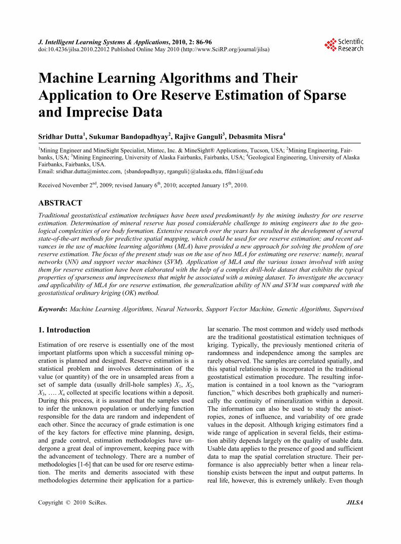
The Nome district is located on the south shore of the Seward Peninsula roughly at latitude 64°30’N and lon-gitude 165°30’W. It is 840 km west of Fairbanks and 860 km northwest of Anchorage (Figure 1). Placer gold at Nome was discovered in 1898. Gold and antimony have been produced from lode deposits in this district, and tungsten concentrates have been produced from re-sidual material above the scheelite-bearing lodes near Nome. Other valuable metals, including iron, copper, bismuth, molybdenum, lead, and zinc, are also reported in the Nome district.

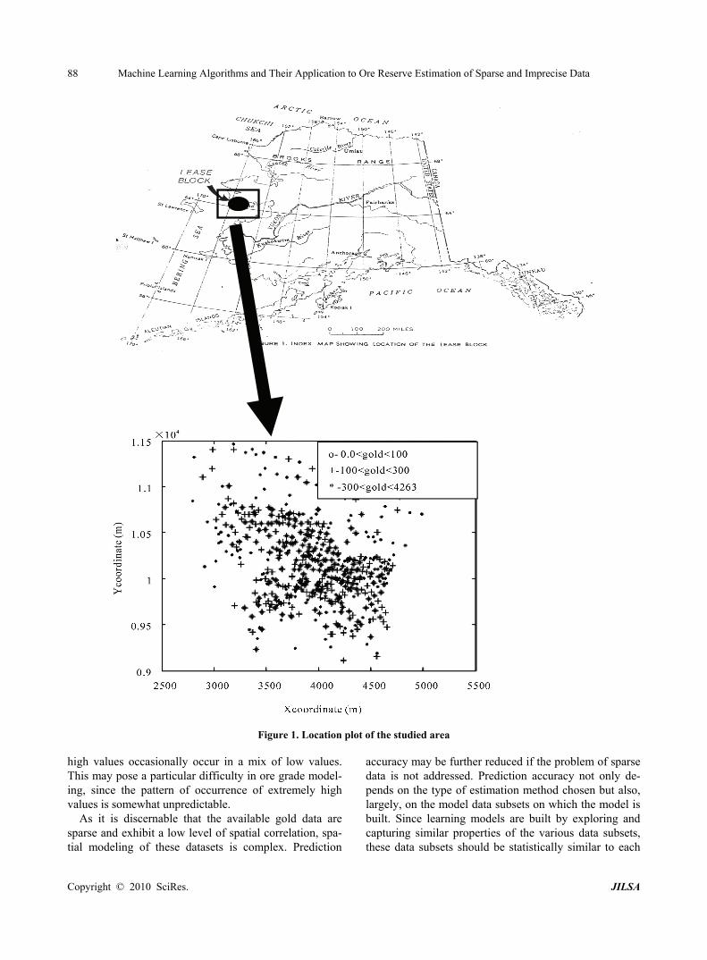
[7] and [8] studied the Nome ore deposit and presented an excellent summary regarding its origins by chroni-cling their exploration and speculating on the chronology of events in the complex regional glacial history that al-lowed the formation and preservation of the deposit. Apart from the research just mentioned, several inde-pendent agencies have carried out exploration work in this area over the last few decades. Figure 2 shows the

composition of the offshore placer gold deposit. Alto-gether, around 3500 exploration drill holes have been made available by the various sampling explorations in the 22,000-acre Nome district. The lease boundary is arbitrarily divided into nine blocks named Coho, Halibut, Herring, Humpy, King, Pink, Red, Silver, and Tomcod. These blocks represent a significant gold resource in the Nome area that could be mined economically.

The present study was conducted in the Red block of the Nome deposit. Four hundred ninety-seven drill-hole samples form the data used for the investigation. Al-though the length of each segment of core sample col-lected from bottom sediment of the sea floor varied con-siderably, the cores were sampled at roughly 1 m inter-vals. On average, each hole was drilled to a depth of 30 m underneath the sea floor. Even though a database com-piled from the core samples of each drill hole was made available, an earlier study by [9] revealed that most of the gold is concentrated within the top 5 m of bottom sedi-ment of the sea floor. As a result, raw drill-hole samples were composited of the first 5 m of sea floor bottom sediment. These drill-hole composites were eventually used for ore grade modeling using NN, SVM, and Geo-statistics.

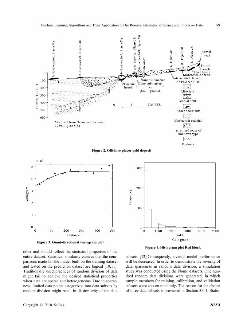
Preliminary statistical analysis conducted on drill-hole composites from the Red block displayed a significantly large grade variation, with a mean and standard deviation of 440.17 mg/m3 and 650.58 mg/m3, respectively. The coefficient of variation is greater than one, which indi-cates the presence of extreme values in the dataset. Spa-tial variability of the dataset was studied and character-ized through a variography study. Figure 3 presents a spatial plot showing an omni-directional variogram for gold concentration in the data set. From the variogram plot, it can be observed that there is a small amount of the regional component. Large proportions of spatial variability occur from the nugget effect, indicating the presence of a poor spatial correlation structure in the de-posit over the study area. Poor spatial correlation, in general, tends to suggest that prediction accuracy for this deposit might not be reliable. Hence, borehole data are sparse for reserve estimation, considering the high spatial variation of ore grade that is commonly associated with placer gold deposit. A histogram plot of the gold data is presented in Figure 4. The histogram plot illustrates that the gold values are positively skewed. A log-normal dis-tribution may be a suitable fit to the data. Visual por-trayal of the histogram plot also reveals that the gold datasets are composed of a large proportion of low values and a small proportion of extremely high values. Closer inspection of the spatial distribution of high and low gold-grade values portrays a distinct spatial characteristic of the deposit. For example, the high values do not ex-

ibit any regular trend. Instead, one or two extremely h



Figure 1. Location plot of the studied area high values occasionally occur in a mix of low values. This may pose a particular difficulty in ore grade model-ing, since the pattern of occurrence of extremely high values is somewhat unpredictable.

As it is discernable that the available gold data are sparse and exhibit a low level of spatial correlation, spa-tial modeling of these datasets is complex. Prediction

accuracy may be further reduced if the problem of sparse data is not addressed. Prediction accuracy not only de-pends on the type of estimation method chosen but also, largely, on the model data subsets on which the model is built. Since learning models are built by exploring and capturing similar properties of the various data subsets, these data subsets should be statistically similar to each



Figure 2. Offshore placer gold deposit

Figure 3. Omni-directional variogram plot other and should reflect the statistical properties of the entire dataset. Statistical similarity ensures that the com-parisons made for the model built on the training dataset and tested on the prediction dataset are logical [10,11]. Traditionally used practices of random division of data might fail to achieve the desired statistical properties when data are sparse and heterogeneous. Due to sparse-ness, limited data points categorized into data subsets by random division might result in dissimilarity of the data

Figure 4. Histogram plot Red block subsets [12].Consequently, overall model performance will be decreased. In order to demonstrate the severity of data sparseness in random data division, a simulation study was conducted using the Nome datasets. One hun-dred random data divisions were generated, in which sample members for training, calibration, and validation subsets were chosen randomly. The reason for the choice of three data subsets is presented in Section 3.0.1. Statis-



tical similarity tests of the three data subsets, using analysis of variance (ANOVA) and Wald tests were conducted. Data division was based on a consideration of all the attributes associated with the deposit, namely, the x-coordinate, y-coordinate, water-table depth, and gold concentration. The results of the simulation study made obvious the fact that almost one-quarter of the data divi-sions are bad during random division of data due to the existing sparseness. This figure can be regarded as quite significant. The unreliability of random data division is further explored through inspection of a bad data division. A statistical summary for one of the arbitrarily selected random data divisions for the dataset is presented in Ta-ble 1. From the table, it is seen that both the mean and standard deviation values are significantly different. Therefore, careful subdivision of data during model de-velopment is essential. Various methodologies were in-vestigated in this regard for proper data subdivision un-der such a modeling framework, including the applica-tion of genetic algorithms (GA) [3,5,13,14] and Koho-nen networks [11,14]. A detailed description of the the-ory and working principle of these methodologies can be found in any NN literature [15,16].

3. Nome Gold Reserve Estimation

When estimating ore grade, northing, easting, and wa-ter-table depth were considered as input variables, and gold grade associated with drill-hole composites up to a depth of 5 m of sea floor was considered an output vari-able. The next few sections describe the application of NN and SVM to ore reserve estimation, along with vari-ous issues that arose while using NN and SVM for ore reserve modeling.

3.1 NN for Grade Estimation

Neural networks form a computational structure inspired by the study of biological neural processing. This structure exhibits certain brain-like capabilities, including per- ception, pattern recognition, and pattern prediction in a variety of situations. As with the brain, information processing is done in parallel using a network of “neurons.” As a result, NN have capabilities that go beyond algo-rithmic programming and work exceptionally well for nonlinear input-output mapping. It is this property of nonlinear mapping that makes NN appealing for ore grade estimation.

There is a fundamental difference in the principles of OK and NN. While OK utilizes information from local samples only, NN utilize information from all of the samples. Ordinary Kriging is regarded as a local estima-tion technique, whereas NN are global estimation tech-niques. If any nonlinear spatial trend is present in a de-posit, it is expected that the NN will capture it reasonably

well. The basic mechanisms of NN have been discussed at length in the literature [15,17]. A brief discussion of NN theory is presented below to provide an overview of the topic.

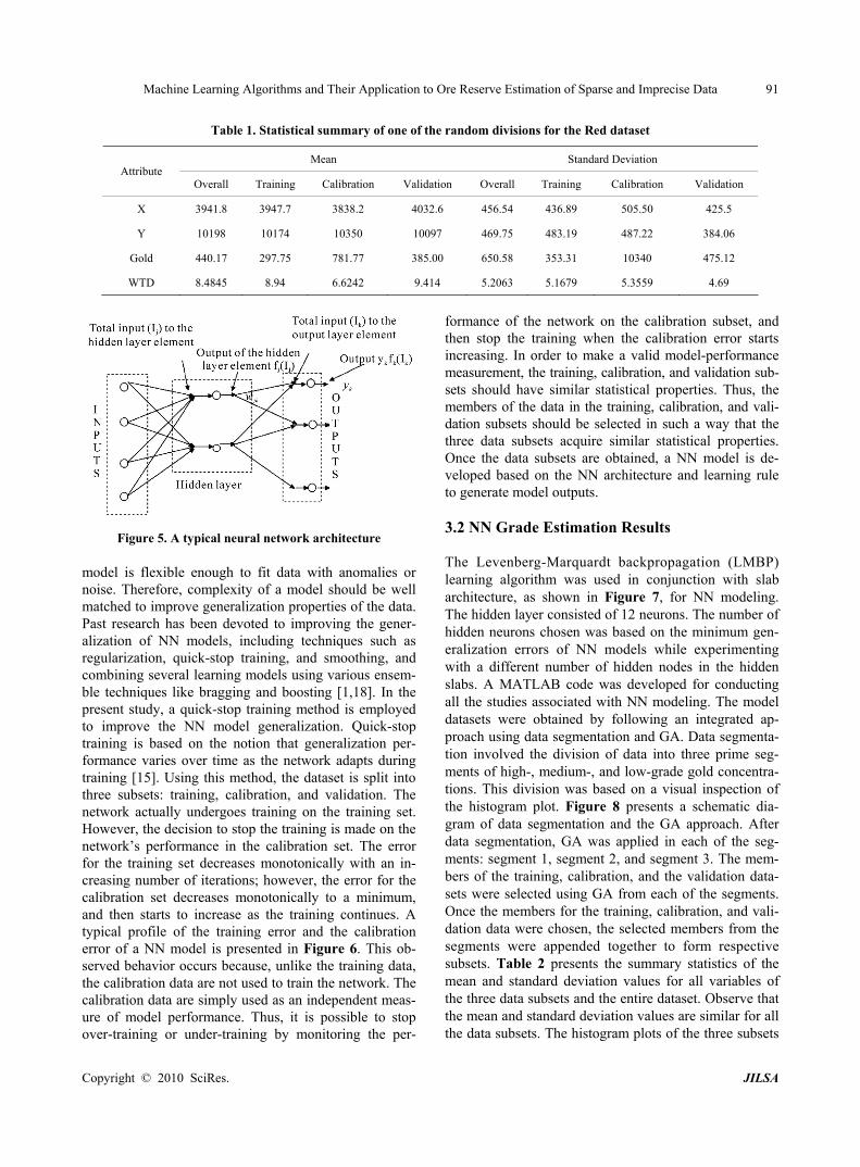
In NN, information is processed through several in- terconnected layers, where each layer is simply repre- sented by a group of elements designated as neurons. Basic NN architecture is made of an input layer consisting of inputs, one or more hidden layers consisting of a number of neurons, and the output layer consisting of outputs. Typical network architecture, having three layers, is presented in Figure 5. Note that while the input layer and the output layer have a fixed number of elements for a given problem, the number of elements in the hidden layer is arbitrary. The basic functioning of NN involves a manipulation of the elements in the input layer and the hidden layer by a weighing function to generate network output. The goodness of the resulting output (how realistic it is) depends upon how each element in the layers is weighted to capture the underlying phe- nomenon. As it is apparent that the weights associated with the interconnections largely decide output accuracy, they must be determined in such a way as to result in minimal error. The process of determination of weights is called learning or training during which, depending upon the output, NN adjust weights iteratively based on their contribution to the error. This process of propagating the effect of the error onto all the weights is called back-propagation. It is during the process of learning that NN map the patterns pre-existing in the data by reflecting the changes in data fluctuations in a spatial coordinate. The sample dataset for a given deposit is used for this pur- pose. Therefore, given the spatial coordinates and other relevant attributes as input and the grade attribute as output, NN will be able to generate a mapping function through a set of connection weights between the input and output. Hence, output, O, of a neural network can be regarded as a function of inputs, X, and connection weights, W: O = (X), where is a mapping function. Training of NN involves finding a good mapping func-tion that maps the input-output patterns correctly. This is done, as previously described, by adjusting connection weights between the neurons of a network, using a suitable learning algorithm while simultaneously fixing the network architecture and activation function.

An additional criterion for optimization of the NN ar-chitecture is to choose the network with minimal gener-alization error. The main goal of NN modeling is not to generate an exact fit to the training data, but to generalize a model that will represent the underlying characteristics of a process. A simple model may result in poor gener-alization, since it can not take into account all the intrica-ies present in the data. On the other hand, a too-complex c



Table 1. Statistical summary of one of the random divisions for the Red dataset

Mean Standard Deviation Attribute

Overall Training Calibration Validation Overall Training Calibration Validation

X 3941.8 3947.7 3838.2 4032.6 456.54 436.89 505.50 425.5

Y 10198 10174 10350 10097 469.75 483.19 487.22 384.06

Gold 440.17 297.75 781.77 385.00 650.58 353.31 10340 475.12

WTD 8.4845 8.94 6.6242 9.414 5.2063 5.1679 5.3559 4.69

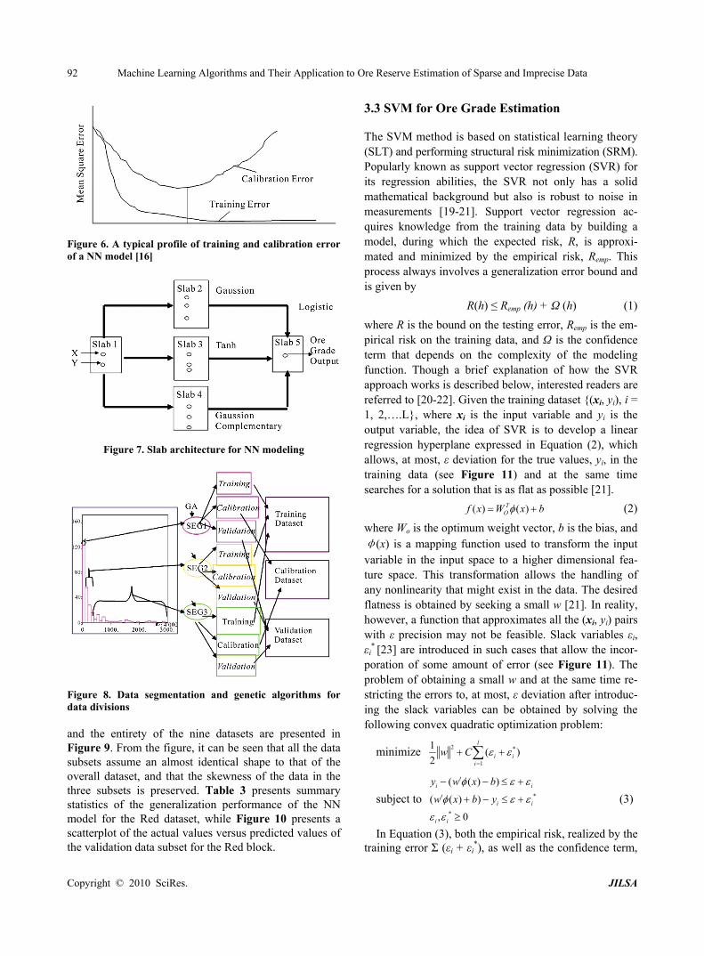
Figure 5. A typical neural network architecture model is flexible enough to fit data with anomalies or noise. Therefore, complexity of a model should be well matched to improve generalization properties of the data. Past research has been devoted to improving the gener-alization of NN models, including techniques such as regularization, quick-stop training, and smoothing, and combining several learning models using various ensem-ble techniques like bragging and boosting [1,18]. In the present study, a quick-stop training method is employed to improve the NN model generalization. Quick-stop training is based on the notion that generalization per-formance varies over time as the network adapts during training [15]. Using this method, the dataset is split into three subsets: training, calibration, and validation. The network actually undergoes training on the training set. However, the decision to stop the training is made on the network’s performance in the calibration set. The error for the training set decreases monotonically with an in-creasing number of iterations; however, the error for the calibration set decreases monotonically to a minimum, and then starts to increase as the training continues. A typical profile of the training error and the calibration error of a NN model is presented in Figure 6. This ob-served behavior occurs because, unlike the training data, the calibration data are not used to train the network. The calibration data are simply used as an independent meas-ure of model performance. Thus, it is possible to stop over-training or under-training by monitoring the per-

formance of the network on the calibration subset, and then stop the training when the calibration error starts increasing. In order to make a valid model-performance measurement, the training, calibration, and validation sub-sets should have similar statistical properties. Thus, the members of the data in the training, calibration, and vali-dation subsets should be selected in such a way that the three data subsets acquire similar statistical properties. Once the data subsets are obtained, a NN model is de-veloped based on the NN architecture and learning rule to generate model outputs.

3.2 NN Grade Estimation Results

The Levenberg-Marquardt backpropagation (LMBP) learning algorithm was used in conjunction with slab architecture, as shown in Figure 7, for NN modeling. The hidden layer consisted of 12 neurons. The number of hidden neurons chosen was based on the minimum gen-eralization errors of NN models while experimenting with a different number of hidden nodes in the hidden slabs. A MATLAB code was developed for conducting all the studies associated with NN modeling. The model datasets were obtained by following an integrated ap-proach using data segmentation and GA. Data segmenta-tion involved the division of data into three prime seg-ments of high-, medium-, and low-grade gold concentra-tions. This division was based on a visual inspection of the histogram plot. Figure 8 presents a schematic dia-gram of data segmentation and the GA approach. After data segmentation, GA was applied in each of the seg-ments: segment 1, segment 2, and segment 3. The mem-bers of the training, calibration, and the validation data-sets were selected using GA from each of the segments. Once the members for the training, calibration, and vali-dation data were chosen, the selected members from the segments were appended together to form respective subsets. Table 2 presents the summary statistics of the mean and standard deviation values for all variables of the three data subsets and the entire dataset. Observe that the mean and standard deviation values are similar for all the data subsets. The histogram plots of the three subsets



Figure 6. A typical profile of training and calibration error of a NN model [16]

Figure 7. Slab architecture for NN modeling

Figure 8. Data segmentation and genetic algorithms for data divisions and the entirety of the nine datasets are presented in Figure 9. From the figure, it can be seen that all the data subsets assume an almost identical shape to that of the overall dataset, and that the skewness of the data in the three subsets is preserved. Table 3 presents summary statistics of the generalization performance of the NN model for the Red dataset, while Figure 10 presents a scatterplot of the actual values versus predicted values of the validation data subset for the Red block.

3.3 SVM for Ore Grade Estimation

The SVM method is based on statistical learning theory (SLT) and performing structural risk minimization (SRM). Popularly known as support vector regression (SVR) for its regression abilities, the SVR not only has a solid mathematical background but also is robust to noise in measurements [19-21]. Support vector regression ac-quires knowledge from the training data by building a model, during which the expected risk, R, is approxi-mated and minimized by the empirical risk, Remp. This process always involves a generalization error bound and is given by

R(h) ≤ Remp (h) + Ω (h) (1)

where R is the bound on the testing error, Remp is the em-pirical risk on the training data, and Ω is the confidence term that depends on the complexity of the modeling function. Though a brief explanation of how the SVR approach works is described below, interested readers are referred to [20-22]. Given the training dataset (xi, yi), i = 1, 2,….L, where xi is the input variable and yi is the output variable, the idea of SVR is to develop a linear regression hyperplane expressed in Equation (2), which allows, at most, ε deviation for the true values, yi, in the training data (see Figure 11) and at the same time searches for a solution that is as flat as possible [21].

( ) ( )TOf x W x b (2)

where Wo is the optimum weight vector, b is the bias, and φ(x) is a mapping function used to transform the input variable in the input space to a higher dimensional fea-ture space. This transformation allows the handling of any nonlinearity that might exist in the data. The desired flatness is obtained by seeking a small w [21]. In reality, however, a function that approximates all the (xi, yi) pairs with ε precision may not be feasible. Slack variables εi, εi

* [23] are introduced in such cases that allow the incor-poration of some amount of error (see Figure 11). The problem of obtaining a small w and at the same time re-stricting the errors to, at most, ε deviation after introduc-ing the slack variables can be obtained by solving the following convex quadratic optimization problem:

minimize 2 *

1

1( )

2

l

i ii

w C

subject to *

*

( ( ) )

( ( ) )

, 0

ti i

ti

i i

y w x b

w x b y i

(3)

In Equation (3), both the empirical risk, realized by the training error Σ (εi + εi

*), as well as the confidence term,




93

Table 2. Statistical summary of data division using GA (Red)

Mean Standard Deviation Attribute

Overall Training Calibration Validation Overall Training Calibration Validation

X 3941.8 3950 3935.6 3931.6 456.54 456.6 457.6 458.6

Y 10198 10194 10218 10186 469.75 471.2 467.2 472.4

Gold 440.17 461.99 418.46 418.59 650.58 673.97 627.89 628.8

WTD 8.4845 8.38 8.63 8.54 5.2063 5.23 5.19 5.19

Figure 11. The soft margin loss settings for linear SVM [21] realized by the ||w||2 term (expressed by Equation (1)) are minimized. An optimum hyperplane is obtained by solv-ing the above minimization problem employing the Kha-rush-Kuhn-Tucker (KKT) conditions [24] which results in minimum generalization error. The final formulation to obtain the SVR model predictions is given by

Figure 9. Histogram plot of Red dataset *

1

*

1

( ) ( ) ( ) ( )

( ) ( , )

i

i

l

i ii

l

i ii

f x x x b

K x x b

(4)

Table 3. Generalization performance of the models for the Red block

Statistics SVM NN OK

Mean Error -8.1 -1.30 33.54

Mean Absolute Error

341.2 351.50 353.02

Root Mean Squared Error 563.13 564.34 565.23

R2 0.234 0.191 0.193

where i, i* are the weights corresponding to individual

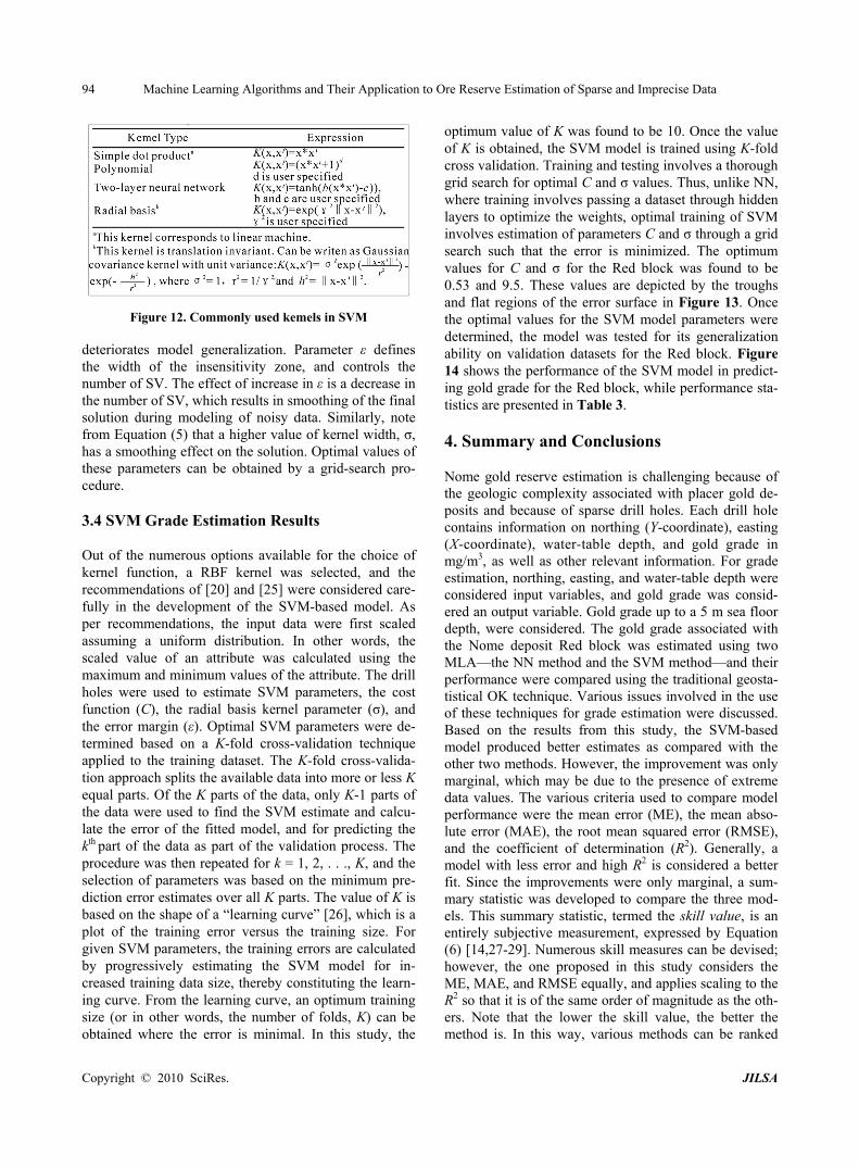
input patterns, K(xi, x) is a user-defined kernel function, and b is the bias parameter. Figure 12 presents a list of commonly used kernels. The most commonly used ker-nel function is an isotropic Gaussian RBF defined by

2

22( , )ix x

iK x x e

(5)

where σ is the kernel bandwidth. The solution of this optimization problem might result in zero weight for some input patterns and non-zero weight for the rest. The patterns with zero weight are redundant and are insig-nificant to the model structure. On the other hand, input patterns with non-zero weights are termed support vec-tors (SV), and they are vital to obtaining model predic-tions. As the number of support vectors increases, so does model complexity. The main parameters that influ-ence SVR model performance are the C, σ, and ε. Pa-rameter C is a trade-off between empirical risk and the weight vector norm ||w||. It decreases empirical risk but, at the same time, increases model complexity, which

Figure 10. Actual vs. predicted for the validation data of Red block


Figure 12. Commonly used kemels in SVM deteriorates model generalization. Parameter ε defines the width of the insensitivity zone, and controls the number of SV. The effect of increase in ε is a decrease in the number of SV, which results in smoothing of the final solution during modeling of noisy data. Similarly, note from Equation (5) that a higher value of kernel width, σ, has a smoothing effect on the solution. Optimal values of these parameters can be obtained by a grid-search pro-cedure.

3.4 SVM Grade Estimation Results

Out of the numerous options available for the choice of kernel function, a RBF kernel was selected, and the recommendations of [20] and [25] were considered care-fully in the development of the SVM-based model. As per recommendations, the input data were first scaled assuming a uniform distribution. In other words, the scaled value of an attribute was calculated using the maximum and minimum values of the attribute. The drill holes were used to estimate SVM parameters, the cost function (C), the radial basis kernel parameter (σ), and the error margin (ε). Optimal SVM parameters were de-termined based on a K-fold cross-validation technique applied to the training dataset. The K-fold cross-valida-tion approach splits the available data into more or less K equal parts. Of the K parts of the data, only K-1 parts of the data were used to find the SVM estimate and calcu-late the error of the fitted model, and for predicting the kth part of the data as part of the validation process. The procedure was then repeated for k = 1, 2, . . ., K, and the selection of parameters was based on the minimum pre-diction error estimates over all K parts. The value of K is based on the shape of a “learning curve” [26], which is a plot of the training error versus the training size. For given SVM parameters, the training errors are calculated by progressively estimating the SVM model for in-creased training data size, thereby constituting the learn-ing curve. From the learning curve, an optimum training size (or in other words, the number of folds, K) can be obtained where the error is minimal. In this study, the

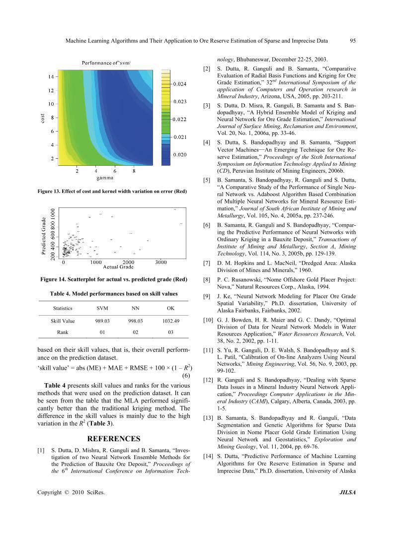
optimum value of K was found to be 10. Once the value of K is obtained, the SVM model is trained using K-fold cross validation. Training and testing involves a thorough grid search for optimal C and σ values. Thus, unlike NN, where training involves passing a dataset through hidden layers to optimize the weights, optimal training of SVM involves estimation of parameters C and σ through a grid search such that the error is minimized. The optimum values for C and σ for the Red block was found to be 0.53 and 9.5. These values are depicted by the troughs and flat regions of the error surface in Figure 13. Once the optimal values for the SVM model parameters were determined, the model was tested for its generalization ability on validation datasets for the Red block. Figure 14 shows the performance of the SVM model in predict-ing gold grade for the Red block, while performance sta-tistics are presented in Table 3.

4. Summary and Conclusions

Nome gold reserve estimation is challenging because of the geologic complexity associated with placer gold de-posits and because of sparse drill holes. Each drill hole contains information on northing (Y-coordinate), easting (X-coordinate), water-table depth, and gold grade in mg/m3, as well as other relevant information. For grade estimation, northing, easting, and water-table depth were considered input variables, and gold grade was consid-ered an output variable. Gold grade up to a 5 m sea floor depth, were considered. The gold grade associated with the Nome deposit Red block was estimated using two MLA—the NN method and the SVM method—and their performance were compared using the traditional geosta-tistical OK technique. Various issues involved in the use of these techniques for grade estimation were discussed. Based on the results from this study, the SVM-based model produced better estimates as compared with the other two methods. However, the improvement was only marginal, which may be due to the presence of extreme data values. The various criteria used to compare model performance were the mean error (ME), the mean abso-lute error (MAE), the root mean squared error (RMSE), and the coefficient of determination (R2). Generally, a model with less error and high R2 is considered a better fit. Since the improvements were only marginal, a sum-mary statistic was developed to compare the three mod-els. This summary statistic, termed the skill value, is an entirely subjective measurement, expressed by Equation (6) [14,27-29]. Numerous skill measures can be devised; however, the one proposed in this study considers the ME, MAE, and RMSE equally, and applies scaling to the R2 so that it is of the same order of magnitude as the oth-ers. Note that the lower the skill value, the better the method is. In this way, various methods can be ranked



Figure 13. Effect of cost and kernel width variation on error (Red)

Figure 14. Scatterplot for actual vs. predicted grade (Red)

Table 4. Model performances based on skill values

Statistics SVM NN OK

Skill Value 989.03 998.03 1032.49

Rank 01 02 03

based on their skill values, that is, their overall perform-ance on the prediction dataset.

‘skill value’ = abs (ME) + MAE + RMSE + 100 × (1 – R2) (6)

Table 4 presents skill values and ranks for the various methods that were used on the prediction dataset. It can be seen from the table that the MLA performed signifi-cantly better than the traditional kriging method. The difference in the skill values is mainly due to the high variation in the R2 (Table 3).

REFERENCES [1] S. Dutta, D. Mishra, R. Ganguli and B. Samanta, “Inves-

tigation of two Neural Network Ensemble Methods for the Prediction of Bauxite Ore Deposit,” Proceedings of the 6th International Conference on Information Tech-

nology, Bhubaneswar, December 22-25, 2003.

[2] S. Dutta, R. Ganguli and B. Samanta, “Comparative Evaluation of Radial Basis Functions and Kriging for Ore Grade Estimation,” 32nd International Symposium of the application of Computers and Operation research in Mineral Industry, Arizona, USA, 2005, pp. 203-211.

[3] S. Dutta, D. Misra, R. Ganguli, B. Samanta and S. Ban-dopadhyay, “A Hybrid Ensemble Model of Kriging and Neural Network for Ore Grade Estimation,” International Journal of Surface Mining, Reclamation and Environment, Vol. 20, No. 1, 2006a, pp. 33-46.

[4] S. Dutta, S. Bandopadhyay and B. Samanta, “Support Vector Machines—An Emerging Technique for Ore Re-serve Estimation,” Proceedings of the Sixth International Symposium on Information Technology Applied to Mining (CD), Peruvian Institute of Mining Engineers, 2006b.

[5] B. Samanta, S. Bandopadhyay, R. Ganguli and S. Dutta, “A Comparative Study of the Performance of Single Neu-ral Network vs. Adaboost Algorithm Based Combination of Multiple Neural Networks for Mineral Resource Esti-mation,” Journal of South African Institute of Mining and Metallurgy, Vol. 105, No. 4, 2005a, pp. 237-246.

[6] B. Samanta, R. Ganguli and S. Bandopadhyay, “Compar-ing the Predictive Performance of Neural Networks with Ordinary Kriging in a Bauxite Deposit,” Transactions of Institute of Mining and Metallurgy, Section A, Mining Technology, Vol. 114, No. 3, 2005b, pp. 129-139.

[7] D. M. Hopkins and L. MacNeil, “Dredged Area: Alaska Division of Mines and Minerals,” 1960.

[8] P. C. Rusanowski, “Nome Offshore Gold Placer Project: Nova,” Natural Resources Corp., Alaska, 1994.

[9] J. Ke, “Neural Network Modeling for Placer Ore Grade Spatial Variability,” Ph.D. dissertation, University of Alaska Fairbanks, Fairbanks, 2002.

[10] G. J. Bowden, H. R. Maier and G. C. Dandy, “Optimal Division of Data for Neural Network Models in Water Resources Application,” Water Resources Research, Vol. 38, No. 2, 2002, pp. 1-11.

[11] S. Yu, R. Ganguli, D. E. Walsh, S. Bandopadhyay and S. L. Patil, “Calibration of On-line Analyzers Using Neural Networks,” Mining Engineering, Vol. 56, No. 9, 2003, pp. 99-102.

[12] R. Ganguli and S. Bandopadhyay, “Dealing with Sparse Data Issues in a Mineral Industry Neural Network Appli-cation,” Proceedings Computer Applications in the Min-eral Industry (CAMI), Calgary, Alberta, Canada, 2003, pp. 1-5.

[13] B. Samanta, S. Bandopadhyay and R. Ganguli, “Data Segmentation and Genetic Algorithms for Sparse Data Division in Nome Placer Gold Grade Estimation Using Neural Network and Geostatistics,” Exploration and Mining Geology, Vol. 11, 2004, pp. 69-76.

[14] S. Dutta, “Predictive Performance of Machine Learning Algorithms for Ore Reserve Estimation in Sparse and Imprecise Data,” Ph.D. dissertation, University of Alaska




96

Fairbanks, Fairbanks, 2006.

[15] M. T. Hagan, H. B. Demuth and M. Beale, “Neural Net-work Design,” PWS Publishing Company, Boston, MA, 1995.

[16] S. Haykins, “Neural Networks: A Comprehensive Foun-dation,” 2nd Edition, Prentice Hall, New Jersey, 1999.

[17] C. M. Bishop, “Neural Networks for Pattern Recogni-tion,” Clarendon Press, Oxford, 1995.

[18] S. Dutta and R. Ganguli, “Application of Boosting Algo-rithm in Neural Network Based Ash Measurement Using Online Ash Analyzers,” 32nd International Symposium of the Application of Computers and Operation Research in Mineral Industry, Arizona, USA, 2005b.

[19] V. Kecman, “Learning and Soft Computing: Support Vector Machines, Neural Network and Fuzzy Logic Models,” MIT Publishers, USA, 2000.

[20] V. Kecman, “Support Vector Machines Basics—An In-troduction Only,” University of Auckland, School of En-gineering Report, New Zealand, 2004.

[21] A. J. Smola and B. Scholkopf, “A Tutorial on Support Vector Regression,” Statistics and Computing, Vol. 14, No. 3, 2004, pp. 199-222.

[22] V. Vapnik, “Statistical Learning Theory,” John Wiley and Sons, New York, 1998.

[23] C. Cortes, and V. Vapnik, “Support Vector Networks,”

Machine Learning, Vol. 20, No. 3, 1995, pp. 273-297.

[24] R. E. Miller, “Optimization-Foundations and Applica-tions,” John Wiley and Sons, New York, 2000.

[25] C. C. Chang and C. Lin, “LIBSVM: A Library for Sup-port Vector Machines,” 2001. Internet Available: http:// www.csie.ntu.edu.tw/~cjlin/libsvm

[26] T. Hastie, R. Tibshirani and J. Friedman, “The Elements of Statistical Learning Theory—Data Mining, Inference and Prediction,” Springer, New York, 2001.

[27] G. Dubois, “European Report on Automatic Mapping Algorithms for Routine and Emergency Monitoring Data,” Office for Official Publications of the European Commu-nities, Luxembourg, 2005.

[28] S. Dutta, R. Ganguli and B. Samanta, “Investigation of two Neural Network Methods in an Automatic Mapping Exercise,” Journal of Applied GIS, Vol. 1, No. 2, 2005a, pp. 1-19.

[29] S. Dutta, R. Ganguli and B. Samanta, “Investigation of two Neural Network Methods in an Automatic Aapping Exercise,” In: G. Dubois, Ed., European Report on Automatic Mapping Algorithms for Routine and Emer-gency Monitoring Data. Report on the Spatial Interpola-tion Comparison (SIC 2004) Exercise, Office for Official Publications of the European Communities, Luxembourg, 2005c.

machine learning algorithms and their application to ore ...machine learning algorithms and their...

Documents