machine learning 2. logistic regression and lda · machine learning machine learning 2. logistic...
TRANSCRIPT
Machine Learning
Machine Learning
2. Logistic Regression and LDA
Lars Schmidt-Thieme
Information Systems and Machine Learning Lab (ISMLL)Institute for Business Economics and Information Systems
& Institute for Computer ScienceUniversity of Hildesheim
http://www.ismll.uni-hildesheim.de
Lars Schmidt-Thieme, Information Systems and Machine Learning Lab (ISMLL), Institute BW/WI & Institute for Computer Science, University of HildesheimCourse on Machine Learning, winter term 2007 1/40
Machine Learning
1. The Classification Problem
2. Logistic Regression
3. Multi-category Targets
4. Linear Discriminant Analysis
Lars Schmidt-Thieme, Information Systems and Machine Learning Lab (ISMLL), Institute BW/WI & Institute for Computer Science, University of HildesheimCourse on Machine Learning, winter term 2007 1/40
Machine Learning / 1. The Classification Problem
Classification / Supervised Learning
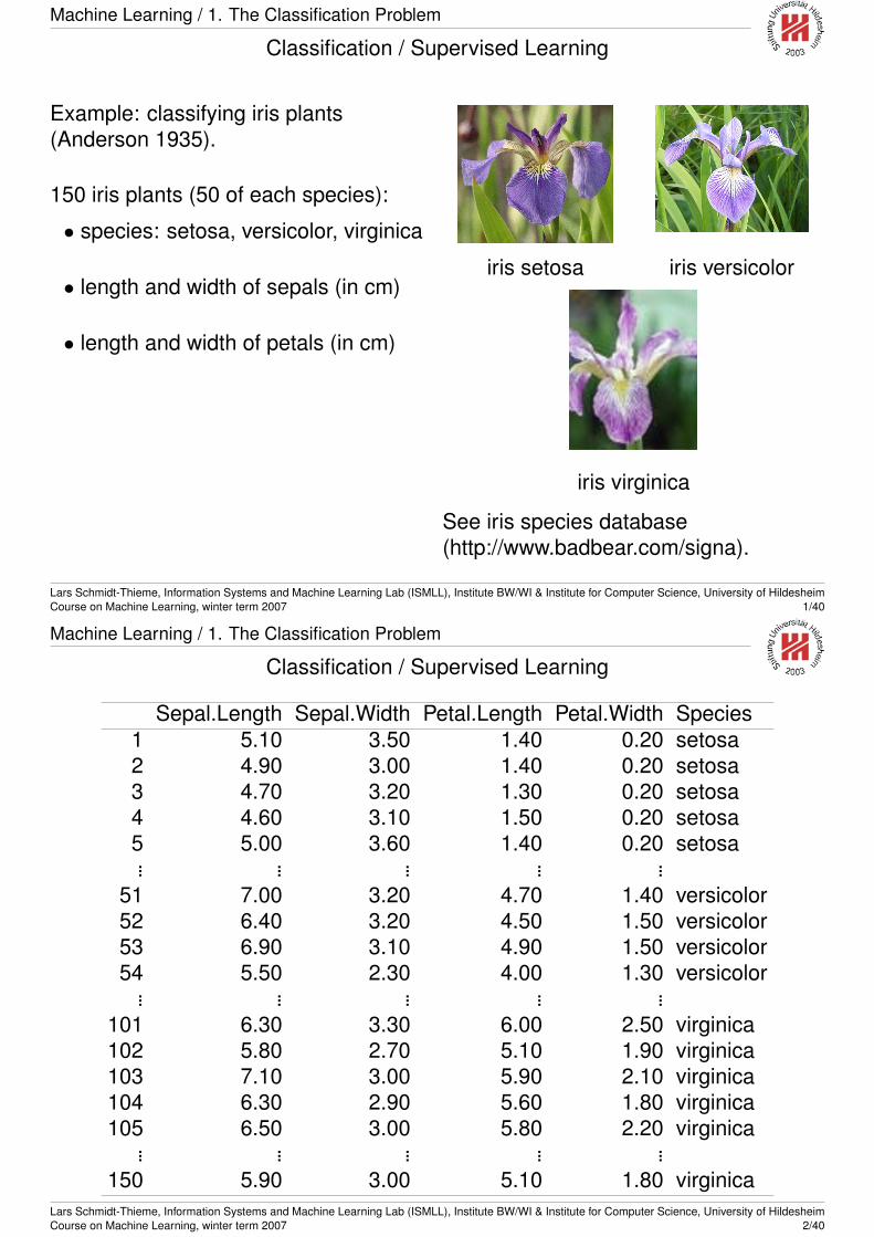
Example: classifying iris plants(Anderson 1935).
150 iris plants (50 of each species):
• species: setosa, versicolor, virginica
• length and width of sepals (in cm)
• length and width of petals (in cm)
iris setosa iris versicolor
iris virginica
See iris species database(http://www.badbear.com/signa).
Lars Schmidt-Thieme, Information Systems and Machine Learning Lab (ISMLL), Institute BW/WI & Institute for Computer Science, University of HildesheimCourse on Machine Learning, winter term 2007 1/40
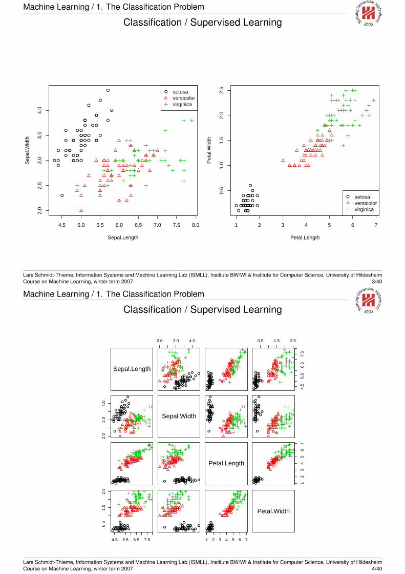
Machine Learning / 1. The Classification Problem
Classification / Supervised Learning
Sepal.Length Sepal.Width Petal.Length Petal.Width Species1 5.10 3.50 1.40 0.20 setosa2 4.90 3.00 1.40 0.20 setosa3 4.70 3.20 1.30 0.20 setosa4 4.60 3.10 1.50 0.20 setosa5 5.00 3.60 1.40 0.20 setosa... ... ... ... ...
51 7.00 3.20 4.70 1.40 versicolor52 6.40 3.20 4.50 1.50 versicolor53 6.90 3.10 4.90 1.50 versicolor54 5.50 2.30 4.00 1.30 versicolor
... ... ... ... ...101 6.30 3.30 6.00 2.50 virginica102 5.80 2.70 5.10 1.90 virginica103 7.10 3.00 5.90 2.10 virginica104 6.30 2.90 5.60 1.80 virginica105 6.50 3.00 5.80 2.20 virginica
... ... ... ... ...150 5.90 3.00 5.10 1.80 virginica
Lars Schmidt-Thieme, Information Systems and Machine Learning Lab (ISMLL), Institute BW/WI & Institute for Computer Science, University of HildesheimCourse on Machine Learning, winter term 2007 2/40
Machine Learning / 1. The Classification Problem
Classification / Supervised Learning
●
●
●
●
●
●
● ●
●
●
●
●
●●
●
●
●
●
●●
●
●
●
●
●
●
●
●
●
●
●
●
●
●
●
●
●
●
●
●
●
●
●
●
●
●
●
●
●
●
4.5 5.0 5.5 6.0 6.5 7.0 7.5 8.0
2.0
2.5
3.0
3.5
4.0
Sepal.Length
Sep
al.W
idth
● setosaversicolorvirginica
●●● ●●
●
●
●●
●
●●
●●
●
●●
● ●●
●
●
●
●
●●
●
●● ●●
●
●
●●●●
●
● ●
●●
●
●
●
●
●●●●
1 2 3 4 5 6 70.
51.
01.
52.
02.
5
Petal.Length
Pet
al.W
idth
● setosaversicolorvirginica
Lars Schmidt-Thieme, Information Systems and Machine Learning Lab (ISMLL), Institute BW/WI & Institute for Computer Science, University of HildesheimCourse on Machine Learning, winter term 2007 3/40
Machine Learning / 1. The Classification Problem
Classification / Supervised Learning
Sepal.Length
2.0 3.0 4.0
●●
●●
●
●
●
●
●
●
●
●●
●
● ●
●
●
●
●
●
●
●
●
●● ●
●●
●●
●●
●
●●
●
●
●
●●
● ●
● ●
●
●
●
●
● ●●●●
●
●
●
●
●
●
●
●●
●
●●
●
●
●
●
●
●
●
●
●●●●●
●●
●●
●
●●
●
●
●
●●
●●
●●
●
●
●
●
●
0.5 1.5 2.5
4.5
5.5
6.5
7.5
●●●●
●
●
●
●
●
●
●
●●
●
● ●
●
●
●
●
●
●
●
●
●● ●●●
●●
●●
●
●●
●
●
●
●●
●●
●●
●
●
●
●
●
2.0
3.0
4.0
●
●
●●
●
●
● ●
●
●
●
●
●●
●
●
●
●
●●
●
●●
●●
●
●●●
●●
●
●●
●●
●●
●
●●
●
●
●
●
●
●
●
●
● Sepal.Width●
●
●●
●
●
●●
●
●
●
●
●●
●
●
●
●
●●
●
●●
●●
●
●●●
●●
●
●●
●●
●●
●
●●
●
●
●
●
●
●
●
●
●
●
●
●●
●
●
●●
●
●
●
●
●●
●
●
●
●
●●
●
●●
●●
●
●●●
●●
●
●●
●●
●●
●
●●
●
●
●
●
●
●
●
●
●
●●●● ●
●● ●● ● ●●
●● ●
●●●
●●
●●
●
●●
●●●●●● ●● ●●
● ●●●●
●●●●●
●●
● ●● ●● ●● ●
●●●● ● ●●
●● ●
●●●
●●
●●
●
●●
● ●●●●● ● ●●●● ●●●
●●● ●●
●
●●
● ●●
Petal.Length
12
34
56
7
●●●●●
●●●●●●●●
●●●●●
●●
●●
●
●●● ●●●●● ●●●●●●
●●●
●●●●
●
●●●●●
4.5 5.5 6.5 7.5
0.5
1.5
2.5
●●●● ●
●●
●●●
●●●●
●
●●● ●●
●
●
●
●
●●
●
●●●●
●
●●●● ●
●● ●
●●●
●
●●
●● ●● ●● ●● ●
●●●●
●●●
●●●
●●● ●●
●
●
●
●
●●
●
●●●●
●
●●●● ●
●● ●
●●●
●
●●
●● ●●
1 2 3 4 5 6 7
●●●●●
●●●●●●●●●
●
●●●●●
●
●
●
●
●●
●
●●●●
●
●●●●●●●●●●●
●
●●●●●●
Petal.Width
Lars Schmidt-Thieme, Information Systems and Machine Learning Lab (ISMLL), Institute BW/WI & Institute for Computer Science, University of HildesheimCourse on Machine Learning, winter term 2007 4/40
Machine Learning
1. The Classification Problem
2. Logistic Regression
3. Multi-category Targets
4. Linear Discriminant Analysis
Lars Schmidt-Thieme, Information Systems and Machine Learning Lab (ISMLL), Institute BW/WI & Institute for Computer Science, University of HildesheimCourse on Machine Learning, winter term 2007 5/40
Machine Learning / 2. Logistic Regression
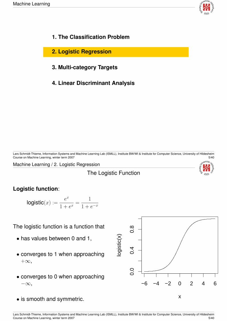
The Logistic Function
Logistic function:
logistic(x) :=ex
1 + ex=
1
1 + e−x
The logistic function is a function that
• has values between 0 and 1,
• converges to 1 when approaching+∞,
• converges to 0 when approaching−∞,
• is smooth and symmetric.
−6 −4 −2 0 2 4 6
0.0
0.4
0.8
x
logi
stic
(x)
Lars Schmidt-Thieme, Information Systems and Machine Learning Lab (ISMLL), Institute BW/WI & Institute for Computer Science, University of HildesheimCourse on Machine Learning, winter term 2007 5/40
Machine Learning / 2. Logistic Regression
The Logit Function
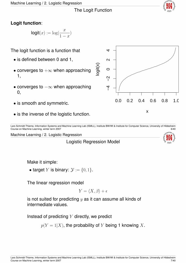
Logit function:
logit(x) := log(x
1− x)
The logit function is a function that
• is defined between 0 and 1,
• converges to +∞ when approaching1,
• converges to −∞ when approaching0,
• is smooth and symmetric.
• is the inverse of the logistic function.
0.0 0.2 0.4 0.6 0.8 1.0
−4
−2
02
4x
logi
t(x)
Lars Schmidt-Thieme, Information Systems and Machine Learning Lab (ISMLL), Institute BW/WI & Institute for Computer Science, University of HildesheimCourse on Machine Learning, winter term 2007 6/40
Machine Learning / 2. Logistic Regression
Logistic Regression Model
Make it simple:
• target Y is binary: Y := {0, 1}.
The linear regression model
Y = 〈X, β〉 + ε
is not suited for predicting y as it can assume all kinds ofintermediate values.
Instead of predicting Y directly, we predict
p(Y = 1|X), the probability of Y being 1 knowing X.
Lars Schmidt-Thieme, Information Systems and Machine Learning Lab (ISMLL), Institute BW/WI & Institute for Computer Science, University of HildesheimCourse on Machine Learning, winter term 2007 7/40
Machine Learning / 2. Logistic Regression
Logistic Regression Model
But linear regression is also not suited for predicting probabilities,as its predicted values are principially unbounded.
Use a trick and transform the unbounded target by a function thatforces it into the unit interval [0, 1], e.g., the logistic function.
Logistic regression model:
p(Y = 1 |X) = logistic(〈X, β〉) + ε =e∑n
i=1 βiXi
1 + e∑n
i=1 βiXi+ ε
Lars Schmidt-Thieme, Information Systems and Machine Learning Lab (ISMLL), Institute BW/WI & Institute for Computer Science, University of HildesheimCourse on Machine Learning, winter term 2007 8/40
Machine Learning / 2. Logistic Regression
A Naive Estimator
A naive estimator could fit the linear regression model to Y(treated as continous target) directly, i.e.,
Y = 〈X, β〉 + ε
and then post-process the linear prediction via
p(Y = 1 |X) = logistic(Y ) = logistic(〈X, β〉) =e∑n
i=1 βiXi
1 + e∑n
i=1 βiXi
But
• β have the property to give minimal RSS for Y ,but what properties do the p(Y = 1 |X) have?
• A probabilistic interpretation requires normal errors for Y ,which is not adequate as Y is bounded to [0, 1].
Lars Schmidt-Thieme, Information Systems and Machine Learning Lab (ISMLL), Institute BW/WI & Institute for Computer Science, University of HildesheimCourse on Machine Learning, winter term 2007 9/40
Machine Learning / 2. Logistic Regression
Maximum Likelihood Estimator
As fit criterium, again the likelihood is used.
As Y is binary, it has a Bernoulli distribution:
Y |X = Bernoulli(p(Y = 1 |X))
Thus, the conditional likelihood function is:
LcondD (β) =
n∏i=1
p(Y = yi |X = xi; β)
=
n∏i=1
p(Y = 1 |X = xi; β)yi(1− p(Y = 1 |X = xi; β))1−yi
Lars Schmidt-Thieme, Information Systems and Machine Learning Lab (ISMLL), Institute BW/WI & Institute for Computer Science, University of HildesheimCourse on Machine Learning, winter term 2007 10/40
Machine Learning / 2. Logistic Regression
Background: Gradient Descent
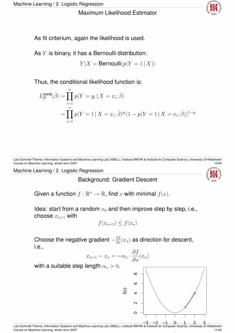
Given a function f : Rn → R, find x with minimal f (x).
Idea: start from a random x0 and then improve step by step, i.e.,choose xn+1 with
f (xn+1) ≤ f (xn)
Choose the negative gradient −∂f∂x(xn) as direction for descent,
i.e.,
xn+1 − xn = −αn ·∂f
∂x(xn)
with a suitable step length αn > 0.
−3 −2 −1 0 1 2 3
02
46
8
x
f(x)
●
Lars Schmidt-Thieme, Information Systems and Machine Learning Lab (ISMLL), Institute BW/WI & Institute for Computer Science, University of HildesheimCourse on Machine Learning, winter term 2007 11/40
Machine Learning / 2. Logistic Regression
Background: Gradient Descent / Example
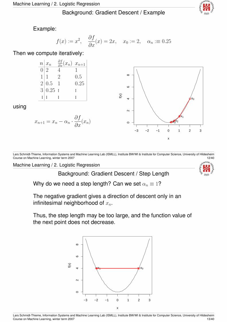
Example:
f (x) := x2,∂f
∂x(x) = 2x, x0 := 2, αn :≡ 0.25
Then we compute iteratively:
n xn∂f∂x(xn) xn+1
0 2 4 11 1 2 0.52 0.5 1 0.253 0.25 ... ...... ... ... ...
using
xn+1 = xn − αn ·∂f
∂x(xn)
−3 −2 −1 0 1 2 30
24
68
x
f(x)
● x0
● x1
● x2● x3
Lars Schmidt-Thieme, Information Systems and Machine Learning Lab (ISMLL), Institute BW/WI & Institute for Computer Science, University of HildesheimCourse on Machine Learning, winter term 2007 12/40
Machine Learning / 2. Logistic Regression
Background: Gradient Descent / Step Length
Why do we need a step length? Can we set αn ≡ 1?
The negative gradient gives a direction of descent only in aninfinitesimal neighborhood of xn.
Thus, the step length may be too large, and the function value ofthe next point does not decrease.
−3 −2 −1 0 1 2 3
02
46
8
x
f(x)
● x0● x1
Lars Schmidt-Thieme, Information Systems and Machine Learning Lab (ISMLL), Institute BW/WI & Institute for Computer Science, University of HildesheimCourse on Machine Learning, winter term 2007 13/40
Machine Learning / 2. Logistic Regression
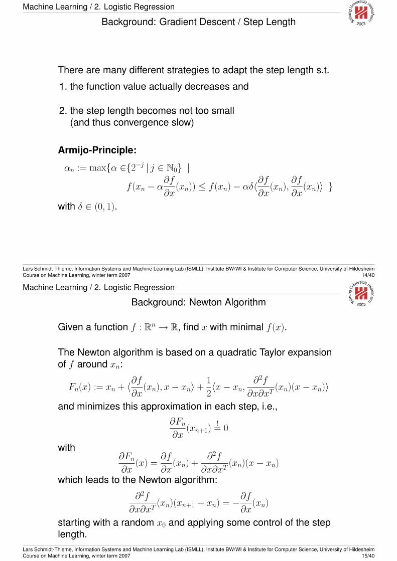
Background: Gradient Descent / Step Length
There are many different strategies to adapt the step length s.t.
1. the function value actually decreases and
2. the step length becomes not too small(and thus convergence slow)
Armijo-Principle:
αn := max{α ∈{2−j | j ∈ N0} |
f (xn − α∂f
∂x(xn)) ≤ f (xn)− αδ〈∂f
∂x(xn),
∂f
∂x(xn)〉 }
with δ ∈ (0, 1).
Lars Schmidt-Thieme, Information Systems and Machine Learning Lab (ISMLL), Institute BW/WI & Institute for Computer Science, University of HildesheimCourse on Machine Learning, winter term 2007 14/40
Machine Learning / 2. Logistic Regression
Background: Newton Algorithm
Given a function f : Rn → R, find x with minimal f (x).
The Newton algorithm is based on a quadratic Taylor expansionof f around xn:
Fn(x) := xn + 〈∂f
∂x(xn), x− xn〉 +
1
2〈x− xn,
∂2f
∂x∂xT(xn)(x− xn)〉
and minimizes this approximation in each step, i.e.,∂Fn
∂x(xn+1)
!= 0
with∂Fn
∂x(x) =
∂f
∂x(xn) +
∂2f
∂x∂xT(xn)(x− xn)
which leads to the Newton algorithm:
∂2f
∂x∂xT(xn)(xn+1 − xn) = −∂f
∂x(xn)
starting with a random x0 and applying some control of the steplength.
Lars Schmidt-Thieme, Information Systems and Machine Learning Lab (ISMLL), Institute BW/WI & Institute for Computer Science, University of HildesheimCourse on Machine Learning, winter term 2007 15/40
Machine Learning / 2. Logistic Regression
Newton Algorithm for the Loglikelihood
LcondD (β) =
n∏i=1
p(Y = 1 |X = xi; β)yi(1− p(Y = 1 |X = xi; β))1−yi
log LcondD (β) =
n∑i=1
yi log p(Y = 1 |X = xi; β) + (1− yi) log(1− p(Y = 1 |X = xi; β))
=
n∑i=1
yi log(e〈xi,β〉
1 + e〈xi,β〉) + (1− yi) log(1− e〈xi,β〉
1 + e〈xi,β〉)
=
n∑i=1
yi(〈xi, β〉 − log(1 + e〈xi,β〉)) + (1− yi) log(1
1 + e〈xi,β〉)
=
n∑i=1
yi(〈xi, β〉 − log(1 + e〈xi,β〉)) + (1− yi)(− log(1 + e〈xi,β〉))
=
n∑i=1
yi〈xi, β〉 − log(1 + e〈xi,β〉)
Lars Schmidt-Thieme, Information Systems and Machine Learning Lab (ISMLL), Institute BW/WI & Institute for Computer Science, University of HildesheimCourse on Machine Learning, winter term 2007 16/40
Machine Learning / 2. Logistic Regression
Newton Algorithm for the Loglikelihood
log LcondD (β) =
n∑i=1
yi〈xi, β〉 − log(1 + e〈xi,β〉)
∂LcondD (β)
∂β=
n∑i=1
yixi −1
1 + e〈xi,β〉e〈xi,β〉xi
=
n∑i=1
xi(yi − p(Y = 1 |X = xi; β))
=XT (y − p)
with
p :=
p(Y = 1 |X = x1; β))...
p(Y = 1 |X = xn; β))
Lars Schmidt-Thieme, Information Systems and Machine Learning Lab (ISMLL), Institute BW/WI & Institute for Computer Science, University of HildesheimCourse on Machine Learning, winter term 2007 17/40
Machine Learning / 2. Logistic Regression
Newton Algorithm for the Loglikelihood
∂LcondD (β)
∂β=XT (y − p)
∂2LcondD (β)
∂β∂βT=
n∑i=1
−xip(Y = 1 |X = xi; β)(1− p(Y = 1 |X = xi; β))xTi
=−n∑
i=1
xixTi p(Y = 1 |X = xi; β)(1− p(Y = 1 |X = xi; β))
=−XTWX
with
W :=
q(x1; β)(1− q(x1; β)) 0 . . . 0
0 . . . 0... . . . ...0 . . . . . . q(xn; β)(1− q(xn; β))
and q(x; β) := P (Y = 1 |X = x; β).
Lars Schmidt-Thieme, Information Systems and Machine Learning Lab (ISMLL), Institute BW/WI & Institute for Computer Science, University of HildesheimCourse on Machine Learning, winter term 2007 18/40
Machine Learning / 2. Logistic Regression
Newton Algorithm for the Loglikelihood
Newton algorithm:
∂2 log L
∂β∂βT(βn)(βn+1 − βn) =− ∂ log L
∂β(βn)
−XTWX(βn+1 − βn) =−XT (y − p)
XTWXβn+1 =XTW(Xβn + W−1(y − p))
Equivalent to a weighted least squares of the “adjusted response”
z := Xβn + W−1(y − p)
on X known as iteratively reweighted least squares (IRLS).
IRLS typically is started at β(0) := 0and uses constant step length 1.
Lars Schmidt-Thieme, Information Systems and Machine Learning Lab (ISMLL), Institute BW/WI & Institute for Computer Science, University of HildesheimCourse on Machine Learning, winter term 2007 19/40
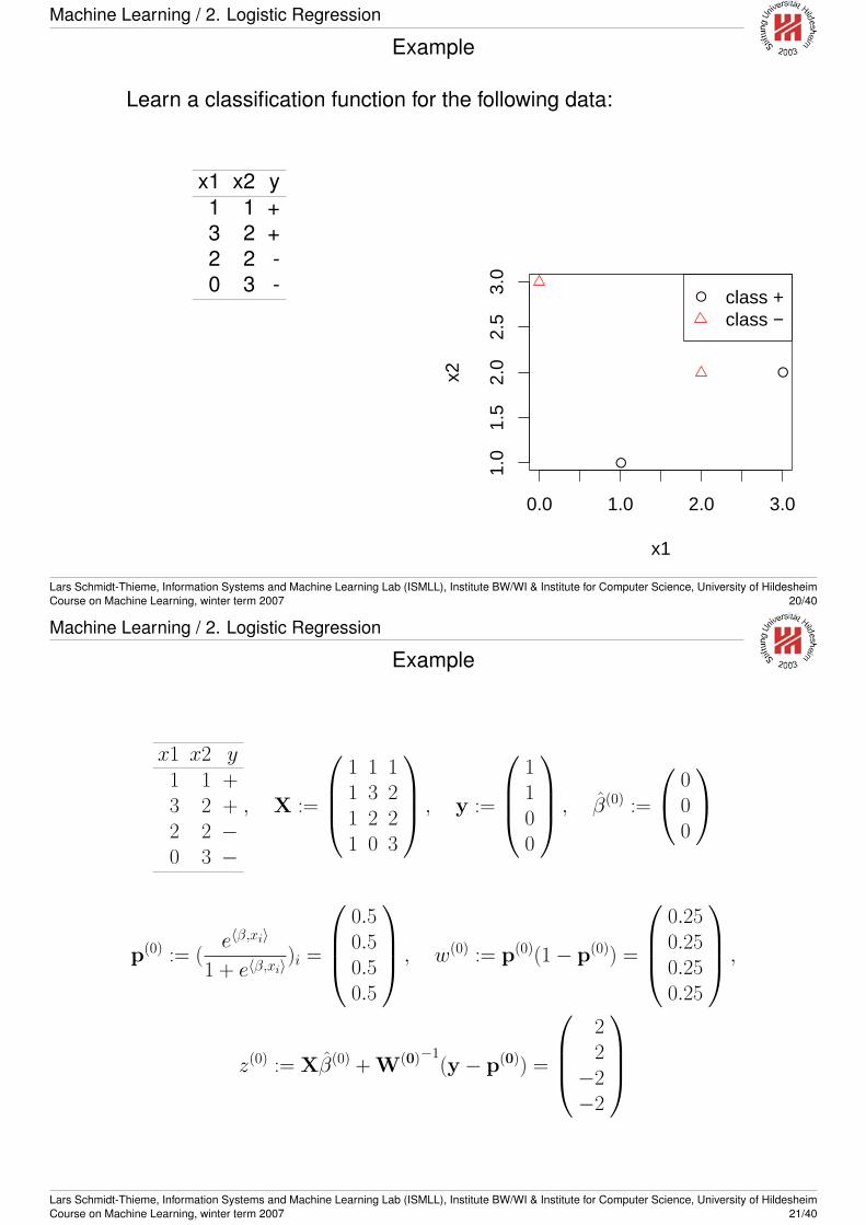
Machine Learning / 2. Logistic Regression
Example
Learn a classification function for the following data:
x1 x2 y1 1 +3 2 +2 2 -0 3 -
●
●
0.0 1.0 2.0 3.01.
01.
52.
02.
53.
0
x1
x2
● class +class −
Lars Schmidt-Thieme, Information Systems and Machine Learning Lab (ISMLL), Institute BW/WI & Institute for Computer Science, University of HildesheimCourse on Machine Learning, winter term 2007 20/40
Machine Learning / 2. Logistic Regression
Example
x1 x2 y1 1 +3 2 +2 2 −0 3 −
, X :=
1 1 11 3 21 2 21 0 3
, y :=
1100
, β(0) :=
000
p(0) := (e〈β,xi〉
1 + e〈β,xi〉)i =
0.50.50.50.5
, w(0) := p(0)(1− p(0)) =
0.250.250.250.25
,
z(0) := Xβ(0) + W(0)−1(y − p(0)) =
22
−2−2
Lars Schmidt-Thieme, Information Systems and Machine Learning Lab (ISMLL), Institute BW/WI & Institute for Computer Science, University of HildesheimCourse on Machine Learning, winter term 2007 21/40
Machine Learning / 2. Logistic Regression
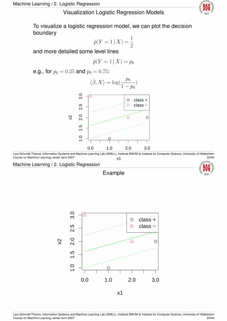
Visualization Logistic Regression Models
To visualize a logistic regression model, we can plot the decisionboundary
p(Y = 1 |X) =1
2and more detailed some level lines
p(Y = 1 |X) = p0
e.g., for p0 = 0.25 and p0 = 0.75:
〈β, X〉 = log(p0
1− p0)
●
●
0.0 1.0 2.0 3.0
1.0
1.5
2.0
2.5
3.0
x1
x2
● class +class −
Lars Schmidt-Thieme, Information Systems and Machine Learning Lab (ISMLL), Institute BW/WI & Institute for Computer Science, University of HildesheimCourse on Machine Learning, winter term 2007 22/40
Machine Learning / 2. Logistic Regression
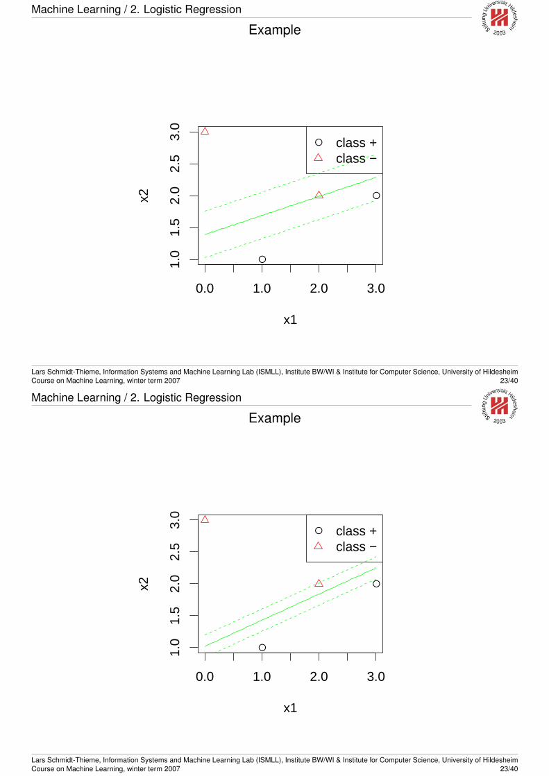
Example
●
●
0.0 1.0 2.0 3.0
1.0
1.5
2.0
2.5
3.0
x1
x2
● class +class −
Lars Schmidt-Thieme, Information Systems and Machine Learning Lab (ISMLL), Institute BW/WI & Institute for Computer Science, University of HildesheimCourse on Machine Learning, winter term 2007 23/40
Machine Learning / 2. Logistic Regression
Example
●
●
0.0 1.0 2.0 3.0
1.0
1.5
2.0
2.5
3.0
x1
x2● class +
class −
Lars Schmidt-Thieme, Information Systems and Machine Learning Lab (ISMLL), Institute BW/WI & Institute for Computer Science, University of HildesheimCourse on Machine Learning, winter term 2007 23/40
Machine Learning / 2. Logistic Regression
Example
●
●
0.0 1.0 2.0 3.0
1.0
1.5
2.0
2.5
3.0
x1
x2
● class +class −
Lars Schmidt-Thieme, Information Systems and Machine Learning Lab (ISMLL), Institute BW/WI & Institute for Computer Science, University of HildesheimCourse on Machine Learning, winter term 2007 23/40
Machine Learning / 2. Logistic Regression
Example
●
●
0.0 1.0 2.0 3.0
1.0
1.5
2.0
2.5
3.0
x1
x2● class +
class −
Lars Schmidt-Thieme, Information Systems and Machine Learning Lab (ISMLL), Institute BW/WI & Institute for Computer Science, University of HildesheimCourse on Machine Learning, winter term 2007 23/40
Machine Learning / 2. Logistic Regression
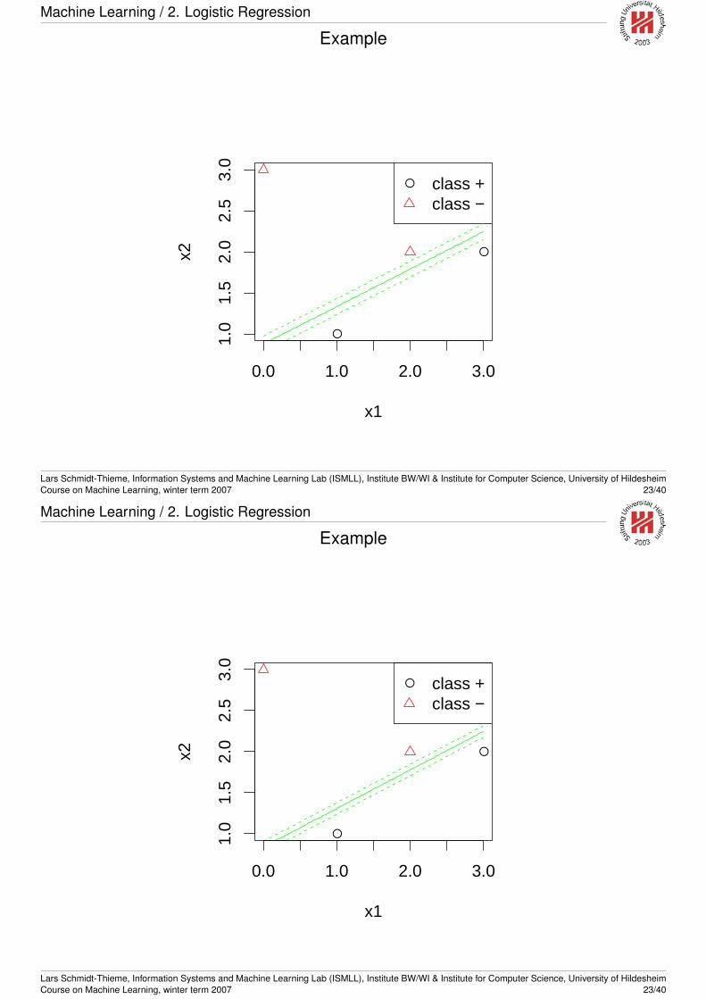
Example
●
●
0.0 1.0 2.0 3.0
1.0
1.5
2.0
2.5
3.0
x1
x2
● class +class −
Lars Schmidt-Thieme, Information Systems and Machine Learning Lab (ISMLL), Institute BW/WI & Institute for Computer Science, University of HildesheimCourse on Machine Learning, winter term 2007 23/40

Machine Learning / 2. Logistic Regression
Example
●
●
0.0 1.0 2.0 3.0
1.0
1.5
2.0
2.5
3.0
x1
x2● class +
class −
Lars Schmidt-Thieme, Information Systems and Machine Learning Lab (ISMLL), Institute BW/WI & Institute for Computer Science, University of HildesheimCourse on Machine Learning, winter term 2007 23/40
Machine Learning / 2. Logistic Regression
Example
●
●
0.0 1.0 2.0 3.0
1.0
1.5
2.0
2.5
3.0
x1
x2
● class +class −
Lars Schmidt-Thieme, Information Systems and Machine Learning Lab (ISMLL), Institute BW/WI & Institute for Computer Science, University of HildesheimCourse on Machine Learning, winter term 2007 23/40
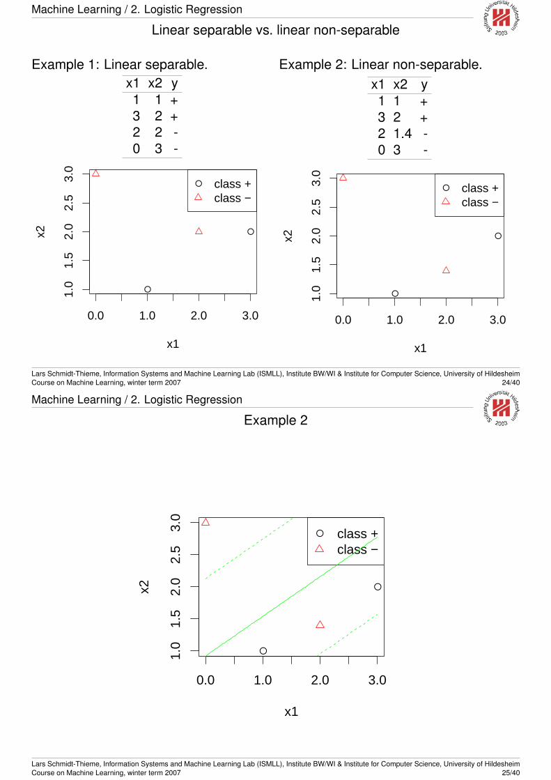
Machine Learning / 2. Logistic Regression
Linear separable vs. linear non-separable
Example 1: Linear separable.x1 x2 y1 1 +3 2 +2 2 -0 3 -
●
●
0.0 1.0 2.0 3.0
1.0
1.5
2.0
2.5
3.0
x1
x2
● class +class −
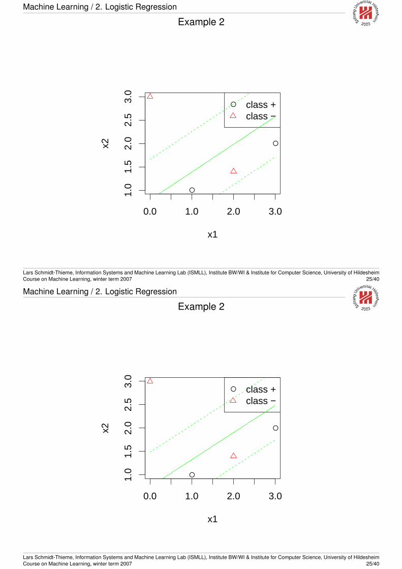
Example 2: Linear non-separable.x1 x2 y1 1 +3 2 +2 1.4 -0 3 -
●
●
0.0 1.0 2.0 3.01.
01.
52.
02.
53.
0
x1
x2
● class +class −
Lars Schmidt-Thieme, Information Systems and Machine Learning Lab (ISMLL), Institute BW/WI & Institute for Computer Science, University of HildesheimCourse on Machine Learning, winter term 2007 24/40
Machine Learning / 2. Logistic Regression
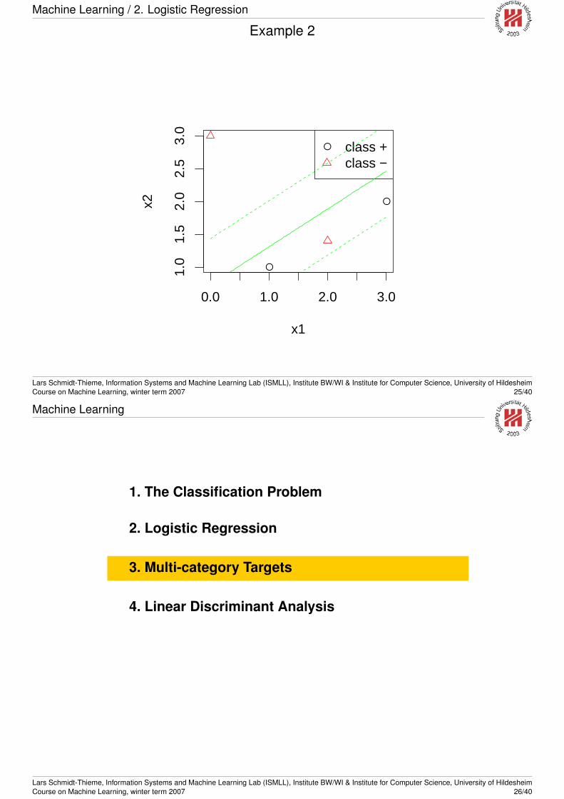
Example 2
●
●
0.0 1.0 2.0 3.0
1.0
1.5
2.0
2.5
3.0
x1
x2
● class +class −
Lars Schmidt-Thieme, Information Systems and Machine Learning Lab (ISMLL), Institute BW/WI & Institute for Computer Science, University of HildesheimCourse on Machine Learning, winter term 2007 25/40
Machine Learning / 2. Logistic Regression
Example 2
●
●
0.0 1.0 2.0 3.0
1.0
1.5
2.0
2.5
3.0
x1
x2● class +
class −
Lars Schmidt-Thieme, Information Systems and Machine Learning Lab (ISMLL), Institute BW/WI & Institute for Computer Science, University of HildesheimCourse on Machine Learning, winter term 2007 25/40
Machine Learning / 2. Logistic Regression
Example 2
●
●
0.0 1.0 2.0 3.0
1.0
1.5
2.0
2.5
3.0
x1
x2
● class +class −
Lars Schmidt-Thieme, Information Systems and Machine Learning Lab (ISMLL), Institute BW/WI & Institute for Computer Science, University of HildesheimCourse on Machine Learning, winter term 2007 25/40
Machine Learning / 2. Logistic Regression
Example 2
●
●
0.0 1.0 2.0 3.0
1.0
1.5
2.0
2.5
3.0
x1
x2● class +
class −
Lars Schmidt-Thieme, Information Systems and Machine Learning Lab (ISMLL), Institute BW/WI & Institute for Computer Science, University of HildesheimCourse on Machine Learning, winter term 2007 25/40
Machine Learning
1. The Classification Problem
2. Logistic Regression
3. Multi-category Targets
4. Linear Discriminant Analysis
Lars Schmidt-Thieme, Information Systems and Machine Learning Lab (ISMLL), Institute BW/WI & Institute for Computer Science, University of HildesheimCourse on Machine Learning, winter term 2007 26/40

Machine Learning / 3. Multi-category Targets
Binary vs. Multi-category Targets
Binary Targets / Binary Classification:prediction of a nominal target variable with 2 levels/values.
Example: spam vs. non-spam.
Multi-category Targets / Multi-class Targets / PolychotomousClassification:prediction of a nominal target variable with more than 2levels/values.
Example: three iris species; 10 digits; 26 letters etc.
Lars Schmidt-Thieme, Information Systems and Machine Learning Lab (ISMLL), Institute BW/WI & Institute for Computer Science, University of HildesheimCourse on Machine Learning, winter term 2007 26/40
Machine Learning / 3. Multi-category Targets
Compound vs. Monolithic Classifiers
Compound models• built from binary submodels,
• different types of compound models employ different sets ofsubmodels:1-vs-rest (aka 1-vs-all)1-vs-last
1-vs-1 (Dietterich and Bakiri 1995; aka pairwise classification)DAG
• using error-correcting codes to combine component models.
• also ensembles of compound models are used(Frank and Kramer 2004).
Monolithic models (aka "‘one machine"’ (Rifkin and Klautau 2004))• trying to solve the multi-class target problem intrinsically
• examples: decision trees, special SVMs, etc.Lars Schmidt-Thieme, Information Systems and Machine Learning Lab (ISMLL), Institute BW/WI & Institute for Computer Science, University of HildesheimCourse on Machine Learning, winter term 2007 27/40
Machine Learning / 3. Multi-category Targets
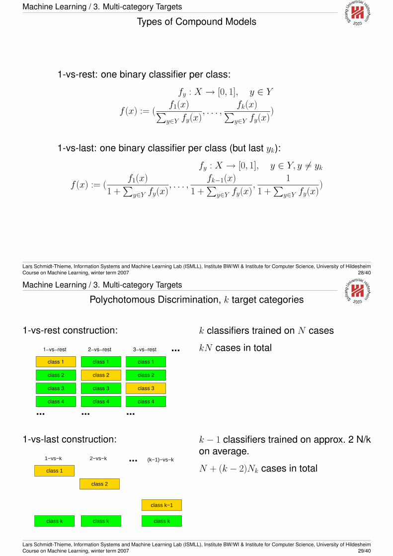
Types of Compound Models
1-vs-rest: one binary classifier per class:
fy : X → [0, 1], y ∈ Y
f (x) := (f1(x)∑
y∈Y fy(x), . . . ,
fk(x)∑y∈Y fy(x)
)
1-vs-last: one binary classifier per class (but last yk):
fy : X → [0, 1], y ∈ Y, y 6= yk
f (x) := (f1(x)
1 +∑
y∈Y fy(x), . . . ,
fk−1(x)
1 +∑
y∈Y fy(x),
1
1 +∑
y∈Y fy(x))
Lars Schmidt-Thieme, Information Systems and Machine Learning Lab (ISMLL), Institute BW/WI & Institute for Computer Science, University of HildesheimCourse on Machine Learning, winter term 2007 28/40
Machine Learning / 3. Multi-category Targets
Polychotomous Discrimination, k target categories
1-vs-rest construction:
class 1
class 2
class 3
class 4
class 1
class 2
class 3
class 4
class 2
class 3
class 4
class 1
2−vs−rest
...
3−vs−rest
...
1−vs−rest
...
...
k classifiers trained on N cases
kN cases in total
1-vs-last construction:
class 2
class 1
class k class k class k
class k−1
2−vs−k1−vs−k (k−1)−vs−k...
k − 1 classifiers trained on approx. 2 N/kon average.
N + (k − 2)Nk cases in total
Lars Schmidt-Thieme, Information Systems and Machine Learning Lab (ISMLL), Institute BW/WI & Institute for Computer Science, University of HildesheimCourse on Machine Learning, winter term 2007 29/40
Machine Learning / 3. Multi-category Targets
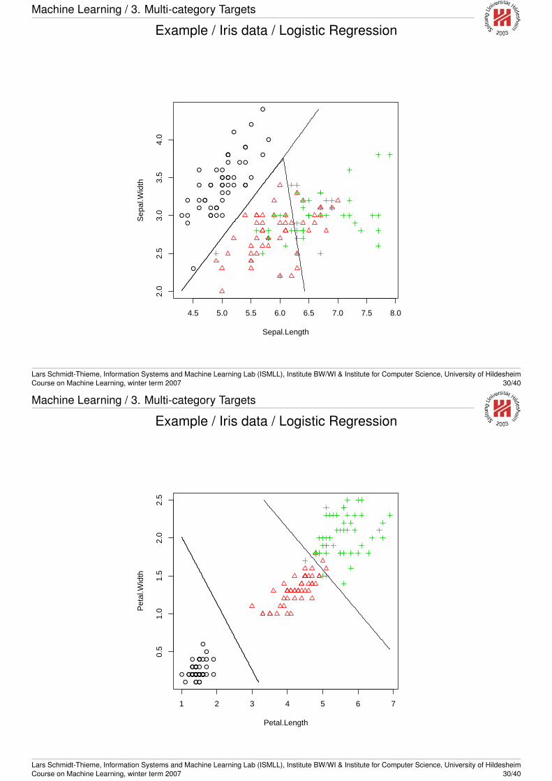
Example / Iris data / Logistic Regression
●
●
●
●
●
●
● ●
●
●
●
●
●●
●
●
●
●
●●
●
●
●
●
●
●
●
●
●
●
●
●
●
●
●
●
●
●
●
●
●
●
●
●
●
●
●
●
●
●
4.5 5.0 5.5 6.0 6.5 7.0 7.5 8.0
2.0
2.5
3.0
3.5
4.0
Sepal.Length
Sep
al.W
idth
Lars Schmidt-Thieme, Information Systems and Machine Learning Lab (ISMLL), Institute BW/WI & Institute for Computer Science, University of HildesheimCourse on Machine Learning, winter term 2007 30/40
Machine Learning / 3. Multi-category Targets
Example / Iris data / Logistic Regression
●●● ●●
●
●
●●
●
●●
●●
●
●●
● ●●
●
●
●
●
●●
●
●● ●●
●
●
●●●●
●
● ●
●●
●
●
●
●
●●●●
1 2 3 4 5 6 7
0.5
1.0
1.5
2.0
2.5
Petal.Length
Pet
al.W
idth
Lars Schmidt-Thieme, Information Systems and Machine Learning Lab (ISMLL), Institute BW/WI & Institute for Computer Science, University of HildesheimCourse on Machine Learning, winter term 2007 30/40
Machine Learning
1. The Classification Problem
2. Logistic Regression
3. Multi-category Targets
4. Linear Discriminant Analysis
Lars Schmidt-Thieme, Information Systems and Machine Learning Lab (ISMLL), Institute BW/WI & Institute for Computer Science, University of HildesheimCourse on Machine Learning, winter term 2007 31/40
Machine Learning / 4. Linear Discriminant Analysis
Assumptions
In discriminant analysis, it is assumed that
• cases of a each class k are generated according to someprobabilities
πk = p(Y = k)
and
• its predictor variables are generated by a class-specificmultivariate normal distribution
X|Y = k ∼ N (µk, Σk)
i.e.pk(x) :=
1
(2π)d2 |Σk|
12
e−12〈x−µk,Σ−1(x−µk)〉
Lars Schmidt-Thieme, Information Systems and Machine Learning Lab (ISMLL), Institute BW/WI & Institute for Computer Science, University of HildesheimCourse on Machine Learning, winter term 2007 31/40
Machine Learning / 4. Linear Discriminant Analysis
Decision Rule
Discriminant analysis predicts as follows:
Y |X = x := argmaxk πkpk(x) = argmaxk δk(x)
with the discriminant functions
δk(x) := −1
2log |Σk| −
1
2〈x− µk, Σ
−1k (x− µk)〉 + log πk
Here,〈x− µk, Σ
−1k (x− µk)〉
is called the Mahalanobis distance of x and µk.
Thus, discriminant analysis can be described as prototypemethod, where
• each class k is represented by a prototype µk and
• cases are assigned the class with the nearest prototype.
Lars Schmidt-Thieme, Information Systems and Machine Learning Lab (ISMLL), Institute BW/WI & Institute for Computer Science, University of HildesheimCourse on Machine Learning, winter term 2007 32/40
Machine Learning / 4. Linear Discriminant Analysis
Maximum Likelihood Parameter Estimates
The maximum likelihood parameter estimates are as follows:
nk :=
n∑i=1
I(yi = k), with I(x = y) :=
{1, if x = y0, else
πk :=nk
n
µk :=1
nk
∑i:yi=k
xi
Σk :=1
nk
∑i:yi=k
(xi − µk)(xi − µk)T
Lars Schmidt-Thieme, Information Systems and Machine Learning Lab (ISMLL), Institute BW/WI & Institute for Computer Science, University of HildesheimCourse on Machine Learning, winter term 2007 33/40
Machine Learning / 4. Linear Discriminant Analysis
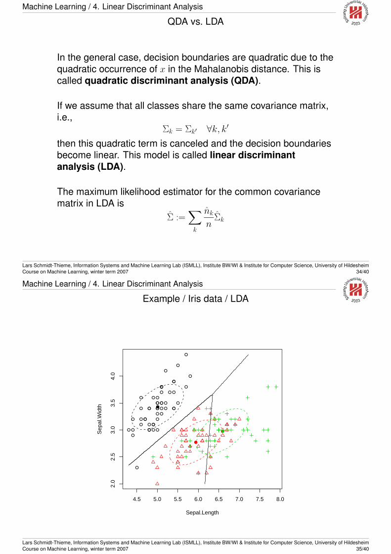
QDA vs. LDA
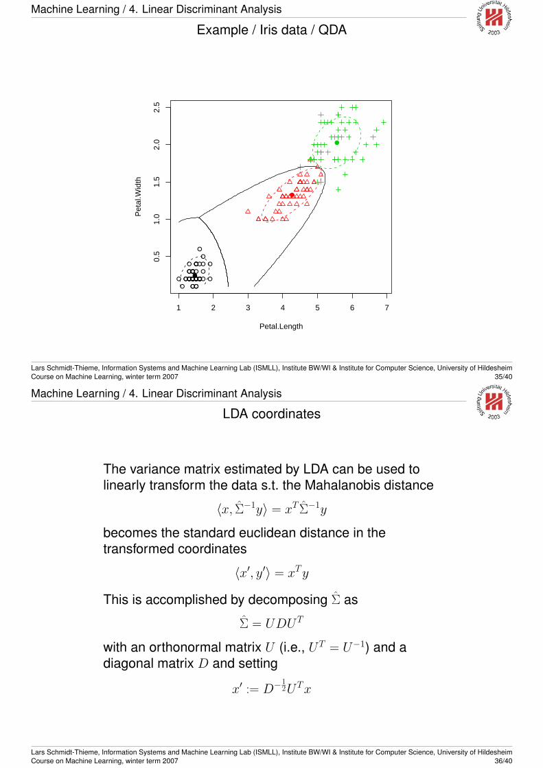
In the general case, decision boundaries are quadratic due to thequadratic occurrence of x in the Mahalanobis distance. This iscalled quadratic discriminant analysis (QDA).
If we assume that all classes share the same covariance matrix,i.e.,
Σk = Σk′ ∀k, k′
then this quadratic term is canceled and the decision boundariesbecome linear. This model is called linear discriminantanalysis (LDA).
The maximum likelihood estimator for the common covariancematrix in LDA is
Σ :=∑
k
nk
nΣk
Lars Schmidt-Thieme, Information Systems and Machine Learning Lab (ISMLL), Institute BW/WI & Institute for Computer Science, University of HildesheimCourse on Machine Learning, winter term 2007 34/40
Machine Learning / 4. Linear Discriminant Analysis
Example / Iris data / LDA
●
●
●
●
●
●
● ●
●
●
●
●
●●
●
●
●
●
●●
●
●
●
●
●
●
●
●
●
●
●
●
●
●
●
●
●
●
●
●
●
●
●
●
●
●
●
●
●
●
4.5 5.0 5.5 6.0 6.5 7.0 7.5 8.0
2.0
2.5
3.0
3.5
4.0
Sepal.Length
Sep
al.W
idth ●
●
●
Lars Schmidt-Thieme, Information Systems and Machine Learning Lab (ISMLL), Institute BW/WI & Institute for Computer Science, University of HildesheimCourse on Machine Learning, winter term 2007 35/40
Machine Learning / 4. Linear Discriminant Analysis
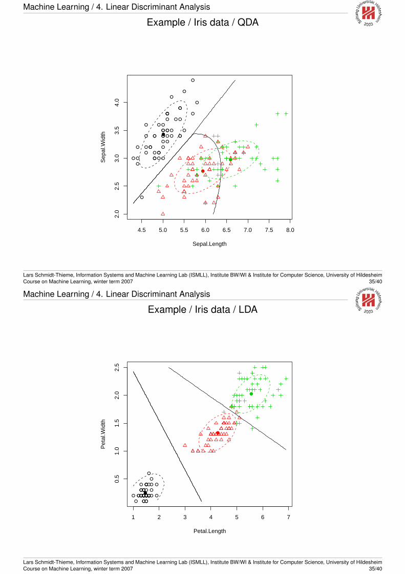
Example / Iris data / QDA
●
●
●
●
●
●
● ●
●
●
●
●
●●
●
●
●
●
●●
●
●
●
●
●
●
●
●
●
●
●
●
●
●
●
●
●
●
●
●
●
●
●
●
●
●
●
●
●
●
4.5 5.0 5.5 6.0 6.5 7.0 7.5 8.0
2.0
2.5
3.0
3.5
4.0
Sepal.Length
Sep
al.W
idth ●
●
●
Lars Schmidt-Thieme, Information Systems and Machine Learning Lab (ISMLL), Institute BW/WI & Institute for Computer Science, University of HildesheimCourse on Machine Learning, winter term 2007 35/40
Machine Learning / 4. Linear Discriminant Analysis
Example / Iris data / LDA
●●● ●●
●
●
●●
●
●●
●●
●
●●
● ●●
●
●
●
●
●●
●
●● ●●
●
●
●●●●
●
● ●
●●
●
●
●
●
●●●●
1 2 3 4 5 6 7
0.5
1.0
1.5
2.0
2.5
Petal.Length
Pet
al.W
idth
●
●
●
Lars Schmidt-Thieme, Information Systems and Machine Learning Lab (ISMLL), Institute BW/WI & Institute for Computer Science, University of HildesheimCourse on Machine Learning, winter term 2007 35/40
Machine Learning / 4. Linear Discriminant Analysis
Example / Iris data / QDA
●●● ●●
●
●
●●
●
●●
●●
●
●●
● ●●
●
●
●
●
●●
●
●● ●●
●
●
●●●●
●
● ●
●●
●
●
●
●
●●●●
1 2 3 4 5 6 7
0.5
1.0
1.5
2.0
2.5
Petal.Length
Pet
al.W
idth
●
●
●
Lars Schmidt-Thieme, Information Systems and Machine Learning Lab (ISMLL), Institute BW/WI & Institute for Computer Science, University of HildesheimCourse on Machine Learning, winter term 2007 35/40
Machine Learning / 4. Linear Discriminant Analysis
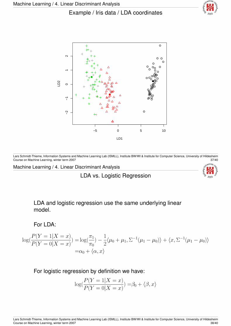
LDA coordinates
The variance matrix estimated by LDA can be used tolinearly transform the data s.t. the Mahalanobis distance
〈x, Σ−1y〉 = xT Σ−1y
becomes the standard euclidean distance in thetransformed coordinates
〈x′, y′〉 = xTy
This is accomplished by decomposing Σ as
Σ = UDUT
with an orthonormal matrix U (i.e., UT = U−1) and adiagonal matrix D and setting
x′ := D−12UTx
Lars Schmidt-Thieme, Information Systems and Machine Learning Lab (ISMLL), Institute BW/WI & Institute for Computer Science, University of HildesheimCourse on Machine Learning, winter term 2007 36/40
Machine Learning / 4. Linear Discriminant Analysis
Example / Iris data / LDA coordinates
●
●
●
●
●
●
●
●
● ●
●
●
●
●
●
●
●
●
●●
●
●
●
●
●
●
●
●●
●
●
●
●
●
●
●
●
●
●
●
●
●
●
●
●
●
●
●
●
●
−5 0 5 10
−2
−1
01
2
LD1
LD2 ●
●
●
Lars Schmidt-Thieme, Information Systems and Machine Learning Lab (ISMLL), Institute BW/WI & Institute for Computer Science, University of HildesheimCourse on Machine Learning, winter term 2007 37/40
Machine Learning / 4. Linear Discriminant Analysis
LDA vs. Logistic Regression
LDA and logistic regression use the same underlying linearmodel.
For LDA:
log(P (Y = 1|X = x)
P (Y = 0|X = x)) = log(
π1
π0)− 1
2〈µ0 + µ1, Σ
−1(µ1 − µ0)〉 + 〈x, Σ−1(µ1 − µ0)〉
=α0 + 〈α, x〉
For logistic regression by definition we have:
log(P (Y = 1|X = x)
P (Y = 0|X = x)) =β0 + 〈β, x〉
Lars Schmidt-Thieme, Information Systems and Machine Learning Lab (ISMLL), Institute BW/WI & Institute for Computer Science, University of HildesheimCourse on Machine Learning, winter term 2007 38/40
Machine Learning / 4. Linear Discriminant Analysis
LDA vs. Logistic Regression
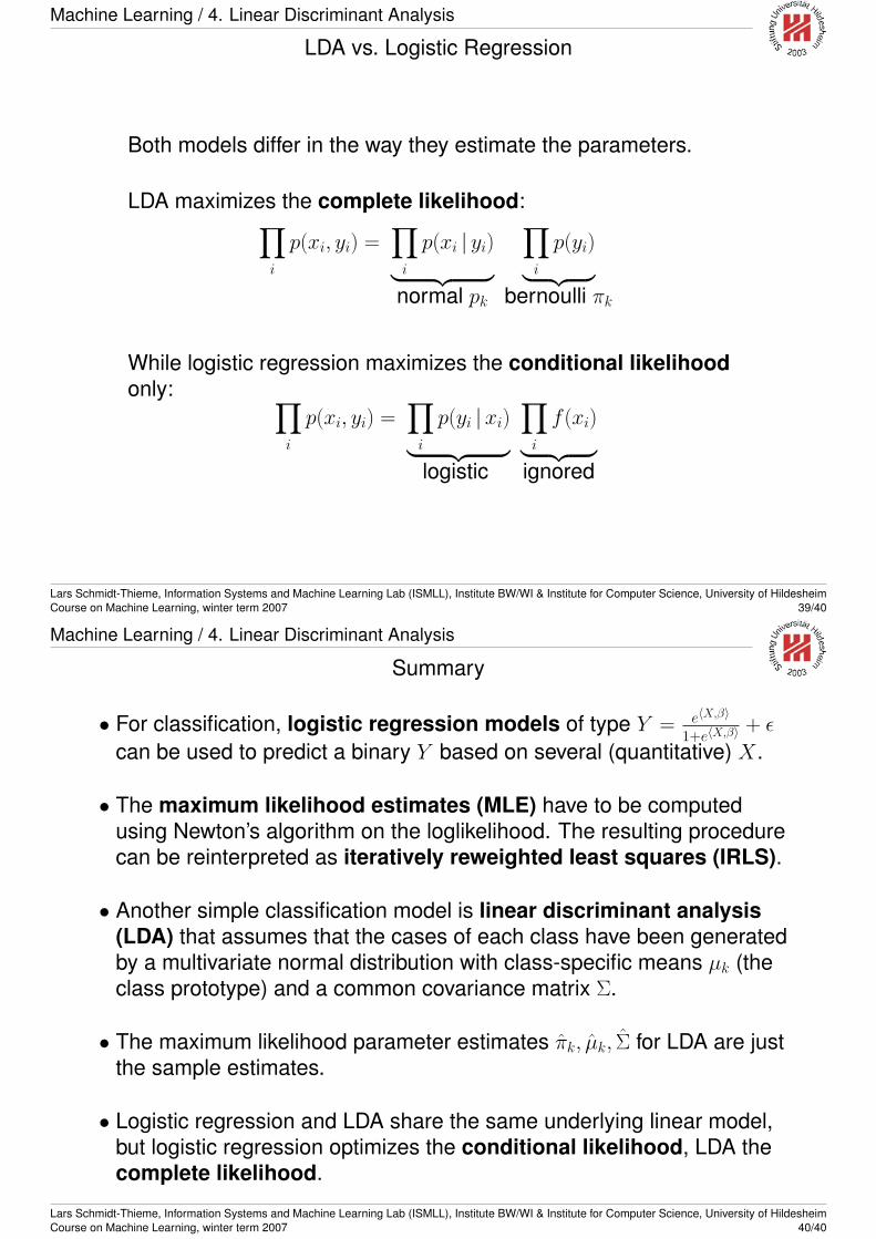
Both models differ in the way they estimate the parameters.
LDA maximizes the complete likelihood:∏i
p(xi, yi) =∏
i
p(xi | yi)︸ ︷︷ ︸∏
i
p(yi)︸ ︷︷ ︸normal pk bernoulli πk
While logistic regression maximizes the conditional likelihoodonly: ∏
i
p(xi, yi) =∏
i
p(yi |xi)︸ ︷︷ ︸∏
i
f (xi)︸ ︷︷ ︸logistic ignored
Lars Schmidt-Thieme, Information Systems and Machine Learning Lab (ISMLL), Institute BW/WI & Institute for Computer Science, University of HildesheimCourse on Machine Learning, winter term 2007 39/40
Machine Learning / 4. Linear Discriminant Analysis
Summary
• For classification, logistic regression models of type Y = e〈X,β〉
1+e〈X,β〉 + ε
can be used to predict a binary Y based on several (quantitative) X.
• The maximum likelihood estimates (MLE) have to be computedusing Newton’s algorithm on the loglikelihood. The resulting procedurecan be reinterpreted as iteratively reweighted least squares (IRLS).
• Another simple classification model is linear discriminant analysis(LDA) that assumes that the cases of each class have been generatedby a multivariate normal distribution with class-specific means µk (theclass prototype) and a common covariance matrix Σ.
• The maximum likelihood parameter estimates πk, µk, Σ for LDA are justthe sample estimates.
• Logistic regression and LDA share the same underlying linear model,but logistic regression optimizes the conditional likelihood, LDA thecomplete likelihood.
Lars Schmidt-Thieme, Information Systems and Machine Learning Lab (ISMLL), Institute BW/WI & Institute for Computer Science, University of HildesheimCourse on Machine Learning, winter term 2007 40/40