macanova users' guide -...
TRANSCRIPT
This file consists of Chapter 3 of MacAnova User’s Guide by Gary W. Oehlert andChristopher Bingham, issued as Technical Report Number 617, School of Statistics,University of Minnesota, revised April 1998, describing Version 4.06 of MacAnova.
This manual is Copyright © 1998 Gary W. Oehlert and Christopher Bingham, all rightsreserved.
Fonts used in this manual are Palatino, Courier, and Symbol.
For information concerning MacAnova, write University of Minnesota, Department ofApplied Statistics, 352 Classroom Office Building, 1994 Buford Avenue, St. Paul, MN55108-6042.
3-0
MacAnova Version 4.06
3. Linear Models
3.1 Introduction to GLM commands One of MacAnova’s greatest strengths is thevariety of commands that perform linear model related computations. Some of themore important are the following:
anova() Unweighted and weighted analysis of variancemanova() Unweighted and weighted multivariate analysis of
varianceregress() Unweighted and weighted simple linear and
multiple regressionscreen() Multiple regression model selectionrobust() Robust regression and ANOVAlogistic() Logistic regressionprobit() Probit regressionpoisson() Poisson regression and log linear model fittingglmfit() Generalized linear model fitting with a variety of
distributions and “links”.
Functions fastanova() and ipf() provide alternatives to anova() and poisson(),respectively, that may be faster in some circumstances.
Some of these commands, such as regress(), anova() and manova(), estimate or fitlinear models ; others such as poisson() and logistic() fit generalized linearmodels (GLM’s). For convenience, we refer to all these commands as GLMcommands , even those that fit truly linear models.
Chapter 10 is almost entirely devoted to examples of the use of GLM commands. Hencethere are relatively few examples in this chapter.
All GLM commands have certain features in common. Chief among these is thespecification of a linear model by a quoted string or CHARACTER variable such as"yield=block+variety+tillage+variety.tillage" or "y=x1+x2+x3+x4". SeeSec. 3. 4.
Another commonality is that all GLM commands create certain variables as side-effects (Sec. 3.6). One of the more important of these is the CHARACTER variableSTRMODEL whose value is the model specification used in the most recent GLMcommand. If you don’t specify a model and STRMODEL exists, GLM commands use themodel specified by STRMODEL.
Other side effect variables created by most GLM commands are SS (sums of squares ordeviances for each term), DF (degrees of freedom), RESIDUALS (response – fitted values)and HII (leverages).
Before a GLM command starts its computations, any side effect variables left over fromprevious linear model commands are deleted. If youwant to retain them, assign themto new variables (residuals1 <- RESIDUALS) before running another GLM com-mand.
In addition, there are several keyword phrases some or all the GLM commands have in
3-1
MacAnova Version 4.06
common (Sec. 3.7).
Sometimes you may want to run a GLM command just to compute the side effectvariables, and don’t want to see the usual output, perhaps because you have seen itbefore. If you use keyword phrase print:F as an argument to any GLM commandexcept screen(), most of the usual output is suppressed. If you use silent:T, alloutput except error messages is suppressed. In both cases the side effect variables suchas RESIDUALS are computed.
The MacAnova interface to all these procedures reflects an underlying similarityamong GLM models. We begin with a discussion of regression and ANOVA, the twomost important methodologies; the other GLM models are postponed to the end ofthis section.
3.2 Response and independent variables in linear models A linear model, includingregression and ANOVA, always has a response variable (also called a dependentvariable or target variable). We refer to the response variable symbolically as Y. Y isassumed to be the sum of a predictable part and an unpredictable part or randomerror. The essence of a linear model is that the predictable part is a linear combinationof one or more other variables (sometimes called the independent variables, predictorvariables or carrier variables) which we refer to here collectively as X-variables.
The random error is always assumed to have zero mean and, in the most commoncase, to have constant variance. This implies that the predictable part is the expectationE[Y]. For the usual regression and ANOVA hypothesis tests and confidenceprocedures to be exact, normal errors are required.
By a linear combination of X-variables X1 ,X2 ,..., Xk , we mean that the predictable partof Y (expectation of Y) has the form
E[Y] = 0 + 1X1 + 2X2 +... + kXk or E[Y] = 1X1 + 2X2 +... + kXk
The first form can be included in the second, if we define X1 to be the variable with 1 asits value for every case. The ’s are referred to as linear model coefficients.Coefficient 0 is the constant term which is often called theintercept and sometimesthe other j’s are called slopes. The random error is simply
e = Y – ( 0 + 1X1 + 2X2 +... + kXk )
Data consist of n cases, with values for Y and the X-variables for each case.regress() and anova() fit a linear model to data using the least squares criterion.This amounts to finding values for the coefficients j of the X-variables so that
Yi − 0 − 1Xi1 − 2Xi 2 −... − kXik( )i
∑ 2,
the sum of squared differences between the observed Y values and the estimatedpredictable part, is as small as possible. For weighted analyses, with weights {W i},
W i Yi − 0 − 1Xi1 − 2Xi 2 −... − kXik( )
i∑ 2
3-2
MacAnova Version 4.06
is minimized. This is appropriate when the variance of the random error for case i isof the form 2/W i, that is the weights are inversely proportional to the errorvariances.
Generalized linear models such as logistic or Poisson regression also involve a fit basedon a linear combination of X-variables, but the expectation of the dependent variable isa (usually) non-linear function of the linear combination. See Chapter 4.
3.3 Variates and factors Although both regression and ANOVA are based on linearmodels, they differ in the type of X-variables used. In regression, the X-variables areusually directly measured or observed numerical variables such as temperature,income or age. In MacAnova, such variables are called variates. In ANOVA, on theother hand, the X-variables code for the levels of categories, for example, treatmentgroups or the blocks in a designed experiment. They may also code the combined levelsof two or more categories. In MacAnova, this distinction is reflected in the fact that forregress(), we specify the actual X-variables to be used, while in anova(), we specifyvariables containing the category levels as positive integers and leave it to MacAnovato figure out how to code the levels in one or more X-variables. Typically to code klevels of a category, MacAnova uses k internally generated X-variables. We callvariables that specify category levels factors to distinguish them from variates.
Since factors and variates are both REAL vectors, function factor() is used to mark avector so that most GLM commands will consider it to be a factor. That is, a REALvector is a variate unless it is specifically declared to be a factor by factor(). Forexample, suppose in a medical experiment involving 7 patients with 4 treatments, A, B,C, D and E, the treatments were assigned as follows:
Patient 1 2 3 4 5 6 7
Treatment A D D C C D B
We create a factor treatment encoding this information by
Cmd> levels <- vector(1,4,4,3,3,4,2) #1=A,2=B,3=C,4=D
Cmd> treatment <- factor(levels)
Cmd> list(levels,treatment) # only treatment is a factorlevels REAL 7 treatment REAL 7 FACTOR with 4 levels
In most subsequent use of treatment GLM model such as "sleep=treatment", it willbe recognized as specifying levels of a factor. However, regress(), screen() andanova() immediately following regress() treat all model variables, includingfactors, as variates.
A subscripted factor remains a factor with the same number of factor levels.
Cmd> treatment1 <- treatment[treatment!=4]; list(treatment1)treatment1 REAL 4 FACTOR with 4 levels
Another way to create a factor is makefactor(values). This transforms the REAL orCHARACTER vector values to a factor with integer levels 1, 2, ... m , where m is thenumber of unique elements in values. The levels assigned by makefactor preserve
3-3
MacAnova Version 4.06
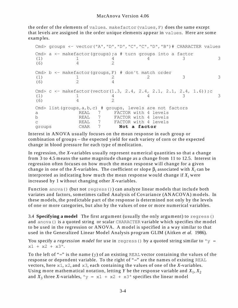
the order of the elements of values. makefactor(values,F) does the same exceptthat levels are assigned in the order unique elements appear in values. Here are someexamples.
Cmd> groups <- vector("A","D","D","C","C","D","B")# CHARACTER values
Cmd> a <- makefactor(groups);a # turn groups into a factor(1) 1 4 4 3 3(6) 4 2
Cmd> b <- makefactor(groups,F) # don't match order(1) 1 2 2 3 3(6) 2 4
Cmd> c <- makefactor(vector(1.3, 2.4, 2.4, 2.1, 2.1, 2.4, 1.6));c(1) 1 4 4 3 3(6) 4 2
Cmd> list(groups,a,b,c) # groups, levels are not factorsa REAL 7 FACTOR with 4 levelsb REAL 7 FACTOR with 4 levelsc REAL 7 FACTOR with 4 levelsgroups CHAR 7 Not a factor
Interest in ANOVA usually focuses on the mean response in each group orcombination of groups – the expected yield for each variety of corn or the expectedchange in blood pressure for each type of medication.
In regression, the X-variables usually represent numerical quantities so that a changefrom 3 to 4.5 means the same magnitude change as a change from 11 to 12.5. Interest inregression often focuses on how much the mean response will change for a givenchange in one of the X-variables. The coefficient or slope i associated with Xi can beinterpreted as indicating how much the mean response would change if Xi wereincreased by 1 without changing other X-variables.
Function anova() (but not regress()) can analyze linear models that include bothvariates and factors, sometimes called Analysis of Covariance (ANACOVA) models. Inthese models, the predictable part of the response is determined not only by the levelsof one or more categories, but also by the values of one or more numerical variables.
3.4 Specifying a model The first argument (usually the only argument) to regress()and anova() is a quoted string or scalar CHARACTER variable which specifies the modelto be used in the regression or ANOVA. A model is specified in a way similar to thatused in the Generalized Linear Model Analysis program GLIM (Aitken et al. 1986).
You specify a regression model for use in regress() by a quoted string similar to "y =x1 + x2 + x3".
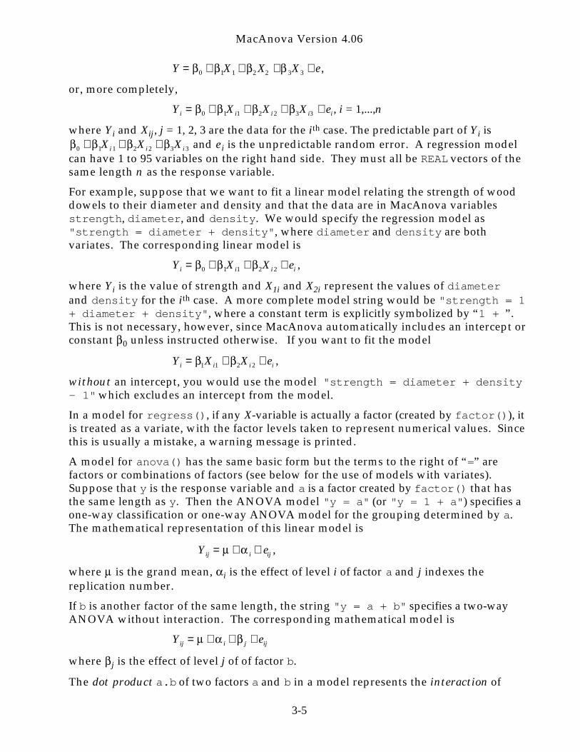
To the left of “=” is the name (y) of an existing REAL vector containing the values of theresponse or dependent variable. To the right of “=” are the names of existing REALvectors, here x1, x2, and x3, each containing the values of one of the X-variables.Using more mathematical notation, letting Y be the response variable and X1, X2and X3 three X-variables, "y = x1 + x2 + x3" specifies the linear model
3-4
MacAnova Version 4.06
Y = 0 + 1X1 + 2 X2 + 3X3 + e ,
or, more completely,
Yi = 0 + 1Xi1 + 2Xi 2 + 3Xi3 + ei , i = 1,...,n
where Yi and Xij , j = 1, 2, 3 are the data for the ith case. The predictable part of Yi is
0 + 1Xi 1 + 2Xi 2 + 3Xi 3 and e i is the unpredictable random error. A regression modelcan have 1 to 95 variables on the right hand side. They must all be REAL vectors of thesame length n as the response variable.
For example, suppose that we want to fit a linear model relating the strength of wooddowels to their diameter and density and that the data are in MacAnova variablesstrength, diameter, and density. We would specify the regression model as"strength = diameter + density", where diameter and density are bothvariates. The corresponding linear model is
Yi = 0 + 1Xi1 + 2Xi 2 + ei ,
where Yi is the value of strength and X1i and X2i represent the values of diameterand density for the ith case. A more complete model string would be "strength = 1+ diameter + density", where a constant term is explicitly symbolized by “1 + ”.This is not necessary, however, since MacAnova automatically includes an intercept orconstant 0 unless instructed otherwise. If you want to fit the model
Yi = 1Xi1 + 2Xi 2 + ei ,
without an intercept, you would use the model "strength = diameter + density- 1" which excludes an intercept from the model.
In a model for regress(), if any X-variable is actually a factor (created by factor()), itis treated as a variate, with the factor levels taken to represent numerical values. Sincethis is usually a mistake, a warning message is printed.
A model for anova() has the same basic form but the terms to the right of “=” arefactors or combinations of factors (see below for the use of models with variates).Suppose that y is the response variable and a is a factor created by factor() that hasthe same length as y. Then the ANOVA model "y = a" (or "y = 1 + a") specifies aone-way classification or one-way ANOVA model for the grouping determined by a.The mathematical representation of this linear model is
Yij = + i + eij ,
where is the grand mean, i is the effect of level i of factor a and j indexes thereplication number.
If b is another factor of the same length, the string "y = a + b" specifies a two-wayANOVA without interaction. The corresponding mathematical model is
Yij = + i + j + eij
where j is the effect of level j of of factor b.
The dot product a.b of two factors a and b in a model represents the interaction of
3-5
MacAnova Version 4.06
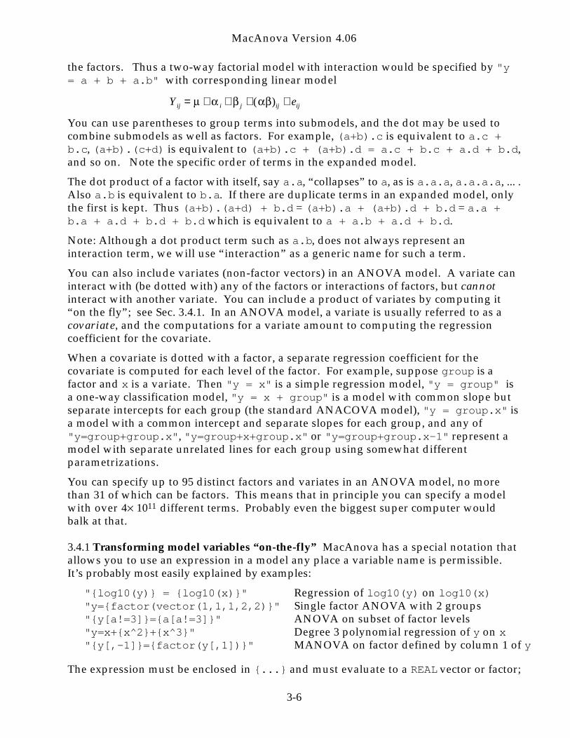
the factors. Thus a two-way factorial model with interaction would be specified by "y= a + b + a.b" with corresponding linear model
Yij = + i + j + ( )ij + eij
You can use parentheses to group terms into submodels, and the dot may be used tocombine submodels as well as factors. For example, (a+b).c is equivalent to a.c +b.c, (a+b).(c+d) is equivalent to (a+b).c + (a+b).d = a.c + b.c + a.d + b.d,and so on. Note the specific order of terms in the expanded model.
The dot product of a factor with itself, say a.a, “collapses” to a, as is a.a.a, a.a.a.a, ... .Also a.b is equivalent to b.a. If there are duplicate terms in an expanded model, onlythe first is kept. Thus (a+b).(a+d) + b.d = (a+b).a + (a+b).d + b.d = a.a +b.a + a.d + b.d + b.d which is equivalent to a + a.b + a.d + b.d.
Note: Although a dot product term such as a.b, does not always represent aninteraction term, we will use “interaction” as a generic name for such a term.
You can also include variates (non-factor vectors) in an ANOVA model. A variate caninteract with (be dotted with) any of the factors or interactions of factors, but cannotinteract with another variate. You can include a product of variates by computing it“on the fly”; see Sec. 3.4.1. In an ANOVA model, a variate is usually referred to as acovariate, and the computations for a variate amount to computing the regressioncoefficient for the covariate.
When a covariate is dotted with a factor, a separate regression coefficient for thecovariate is computed for each level of the factor. For example, suppose group is afactor and x is a variate. Then "y = x" is a simple regression model, "y = group" isa one-way classification model, "y = x + group" is a model with common slope butseparate intercepts for each group (the standard ANACOVA model), "y = group.x" isa model with a common intercept and separate slopes for each group, and any of"y=group+group.x", "y=group+x+group.x" or "y=group+group.x-1" represent amodel with separate unrelated lines for each group using somewhat differentparametrizations.
You can specify up to 95 distinct factors and variates in an ANOVA model, no morethan 31 of which can be factors. This means that in principle you can specify a modelwith over 4 1011 different terms. Probably even the biggest super computer wouldbalk at that.
3.4.1 Transforming model variables “on-the-fly” MacAnova has a special notation thatallows you to use an expression in a model any place a variable name is permissible.It’s probably most easily explained by examples:
"{log10(y)} = {log10(x)}" Regression of log10(y) on log10(x)"y={factor(vector(1,1,1,2,2)}" Single factor ANOVA with 2 groups"{y[a!=3]}={a[a!=3]}" ANOVA on subset of factor levels"y=x+{x^2}+{x^3}" Degree 3 polynomial regression of y on x"{y[,-1]}={factor(y[,1])}" MANOVA on factor defined by column 1 of y
The expression must be enclosed in {...} and must evaluate to a REAL vector or factor;
3-6
MacAnova Version 4.06
on the left side of “=” it can evaluate to a REAL matrix. The expression can be arbitrarilycomplicated and can even consist of several commands separated by semicolons, inwhich case the value of {...} is the value of the last expression. It is an error for the{...} expression to run a GLM command such as regress() or anova().
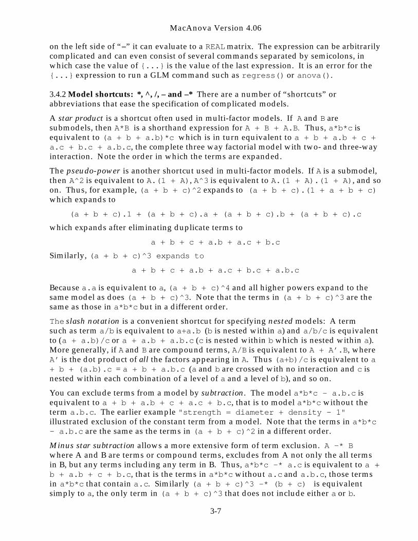
3.4.2 Model shortcuts: *, ^, /, – and –* There are a number of “shortcuts” orabbreviations that ease the specification of complicated models.
A star product is a shortcut often used in multi-factor models. If A and B aresubmodels, then A*B is a shorthand expression for A + B + A.B. Thus, a*b*c isequivalent to (a + b + a.b)*c which is in turn equivalent to a + b + a.b + c +a.c + b.c + a.b.c, the complete three way factorial model with two- and three-wayinteraction. Note the order in which the terms are expanded.
The pseudo-power is another shortcut used in multi-factor models. If A is a submodel,then A^2 is equivalent to A.(1 + A), A^3 is equivalent to A.(1 + A).(1 + A), and soon. Thus, for example, (a + b + c)^2 expands to (a + b + c).(1 + a + b + c)which expands to
(a + b + c).1 + (a + b + c).a + (a + b + c).b + (a + b + c).c
which expands after eliminating duplicate terms to
a + b + c + a.b + a.c + b.c
Similarly, (a + b + c)^3 expands to
a + b + c + a.b + a.c + b.c + a.b.c
Because a.a is equivalent to a, (a + b + c)^4 and all higher powers expand to thesame model as does (a + b + c)^3. Note that the terms in (a + b + c)^3 are thesame as those in a*b*c but in a different order. The slash notation is a convenient shortcut for specifying nested models: A termsuch as term a/b is equivalent to a+a.b (b is nested within a) and a/b/c is equivalentto (a + a.b)/c or a + a.b + a.b.c (c is nested within b which is nested within a).More generally, if A and B are compound terms, A/B is equivalent to A + A’.B, whereA’ is the dot product of all the factors appearing in A. Thus (a+b)/c is equivalent to a+ b + (a.b).c = a + b + a.b.c (a and b are crossed with no interaction and c isnested within each combination of a level of a and a level of b), and so on.
You can exclude terms from a model by subtraction. The model a*b*c - a.b.c isequivalent to a + b + a.b + c + a.c + b.c, that is to model a*b*c without theterm a.b.c. The earlier example "strength = diameter + density - 1"illustrated exclusion of the constant term from a model. Note that the terms in a*b*c- a.b.c are the same as the terms in (a + b + c)^2 in a different order.
Minus star subtraction allows a more extensive form of term exclusion. A -* Bwhere A and B are terms or compound terms, excludes from A not only the all termsin B, but any terms including any term in B. Thus, a*b*c -* a.c is equivalent to a +b + a.b + c + b.c, that is the terms in a*b*c without a.c and a.b.c, those termsin a*b*c that contain a.c. Similarly (a + b + c)^3 -* (b + c) is equivalentsimply to a, the only term in (a + b + c)^3 that does not include either a or b.
3-7
MacAnova Version 4.06
3.4.3 Polynomial and periodic regressions There are additional shortcuts for polynomialand periodic regression. Again these are best illustrated by example:
"y=P4(u)" "y={u}+{(u)^2}+{(u)^3}+{(u)^4}""y=P3(sqrt(x))" "y={sqrt(x)}+{(sqrt(x))^2}+{(sqrt(x))^3}""y=C2(2*PI*hour/24)" "y={cos(2*PI*hour/24)}+{sin(2*PI*hour/24)}+
{cos(2*(2*PI*hour/24))}+{sin(2*(2*PI*hour/24))}
Pn(expr) expands to a sum of n {...} terms (see Sec. 3.4.1) each of which evaluatesto a power of expr. Its primary purpose is to make polynomial regression easier. SeeSec. 10.6 for an example of the use of Pn(expr).
Cn(expr) expands to a sum of n pairs of {...} terms. Pair j evaluates to{cos(j*(expr))}+{sin(j*(expr))}. Typically, as in the example above, expr is alinear function of a variable containing time determinations. In that case,"y=Cn (expr)" is a model specifying a periodic regression. Specifically, if tt is a REALvector of times, y is a REAL vector of responses with y[i] determined at time tt[i]and Per a positive REAL scalar, then "y=Cn(2*PI*tt/Per)" is an periodic regressionmodel with period Per containing cosine and sine terms with periods Per, Per/2, ...,Per/n . When the value of option angles is "degrees", use "y=Cn(360*tt/Per)";when option angles is "cycles", use "y=Cn(tt/Per)".
3.5 Error terms All sums of squares and degrees of freedom that are not contained inany model term are combined into a term usually named ERROR1. Since someANOVA models, such as split plot models, have more than one error term, it is aconvenience to be able to specify other terms as error terms.
Any simple term (a factor or variate or a single dot product of factors or variates) maybe relabeled as an error term by enclosing it in E(). This will affect only the labelling ofthe term in the output, and the numbering of other error terms. Sums of squares arecomputed as usual. For example, anova("y = a + b + a.b") and anova("y = a +b + E(a.b)") specify identical computations, but the term that was labelled a.b in thefirst is labelled ERROR1 in the second and the final line is labelled ERROR2 instead ofERROR1. Following a linear model command, certain commands such as contrast()(see Sec. 3.16) and secoefs() (see Sec. 3.13) allow you to specify which error term is tobe used in computing standard errors. In addition, if you use either fstats:T orpvalues:T on anova(), the denominator of the F-test for each term is taken from thenext following error term.
3-8
MacAnova Version 4.06
3.6 Side effect variables Both regress() and anova() set several side-effect variables:Name Type ContentsSTRMODEL CHARACTER scalar The model usedDEPVNAME CHARACTER scalar The name of the response variableTERMNAMES CHARACTER vector The names of the terms in the modelSS REAL vector Sums of squares for each term in the modelDF REAL vector Degrees of freedom for each term in the
modelRESIDUALS REAL vector Residuals from the model fitHII REAL vector The leverages – the diagonal elements of the
hat matrix H = X( ′ X X)−1 ′ X or, for weightedanalysis, H = X( ′ X WX)−1 ′ X W , where W isdiagonal matrix of weights.
Side effect variables set by regress() but not by anova():
COEF REAL vector The regression coefficientsXTXINV REAL matrix ( ′ X X )−1, where X is the matrix whose
columns are the independent variables,including a constant column if there is anintercept, or ( ′ X WX)−1 , for weightedanalyses.
Side effect variable set by regress() or anova() when weights are specified:
WTDRESIDUALS REAL vector W i residuals from the model fit
All side-effect variables except STRMODEL are deleted at the start of each use ofregress(), anova() or any GLM command. If you want to save a side effect variable,you should assign it to a variable with a different name (for example, residuals <-RESIDUALS) before running another GLM command.
The elements of HII are useful, among other reasons, because V[ri] = (1 - h ii) 2, where
ri is the ith residual (V[ W i ri] = (1 - h ii) 2 for weighted analysis).
3.7 GLM keywords Another area of commonality among the various GLM commandsis the use of keywords. Here is a summary of the keyword phrases shared by more thanone GLM command.
Keyword Phrase Limitations and brief descriptionprint:F All GLM commands. Directs that most of the output to the screen
is suppressed, although side effect variables are created.
silent:T All GLM commands but screen(). Directs that all output excepterror messages is suppressed; only side effect variables arecomputed.
coefs:F All GLM commands but screen(), regress(), fastanova(),ipf(), robust(). Directs that no computation of coefficients or ageneralized inverse to ′ X X is done. Except in the case of balanced
3-9
MacAnova Version 4.06
ANOVA, coefs() and secoefs() cannot be used to retrievecoefficients later. coefs:F can’t be used with marginal:T.
fstats:T regress(), anova(), manova(), robust(). Directs that F-statistics and P values are computed and printed. Thedenominator is the mean square for the next following termwhose name is of the form ERROR1, ERROR2, .... For manova(),ANOVA tables with F-statistics are given separately for eachvariable and printing of the SS/SP matrices is suppressed.fstats:F suppresses F-statistics when they might otherwise beprinted.
pvals:T All GLM commands except screen(). Directs that F or 2 Pvalues are computed and printed for F-statistics, t-statistics, anddeviances. pvals:F suppresses P values when they mightotherwise be printed.
wts:vec anova(), manova(), regress(). Specifies a REAL vector to beweights:vec used as weights. Keywords wts and weights are synonyms.
marginal:T anova(), manova(), robust(). Specifies that SS (or SS/SPmatrices) are computed marginally. When there are no emptycells, and sometimes when there are, the computed SS or SS/SPare usually equivalent to SAS Type III quantities. marginal:T isnot legal with coefs:F. See Sec. 3.11 for details.
increment:T poisson(), ipf(), logistic(), glmfit(). Specifies that anincremental analysis of deviance table with an entry for each termis to be computed and printed. See Sec. 4.2.3.
offset:vec poisson(), ipf(), robust(). Specifies a REAL vector to be usedas offset vector. See Sec. 4.2.3.
maxit:n fastanova(), poisson(), ipf(), logistic(), robust(),glmfit(). Specifies the maximum number of iterations allowedin fitting. See Sec. 4.2.
eps:smallVal fastanova(), poisson(), ipf(), logistic(), robust(),glmfit(). Specifies the a threshold in relative change ofobjective function for determining when convergence has beenreached. See Sec. 4.2.
You can change the default value behavior of most GLM commands to have fstats:Tand/or pvals:T by setoptions(pvals:T,fstat:T). See Sec. 8.1.3.
3.8 anova() and regress() output Functions regress() and anova() return only aNULL value. Instead, they print out standard summaries of their actions and create orupdate “side-effect” variables.
The standard output produced by regress() includes the regression coefficients, theirstandard errors and t-statistics, the coefficient of determination R2, the overallregression F-statistic (excluding the constant term), the mean square error, the errordegrees of freedom and the Durbin-Watson statistic. Typing anova() (with no model)
3-10
MacAnova Version 4.06
immediately after regress(Model) prints an ANOVA table for the regression withoutrecomputing anything. When a regression X-variable is a factor, it is still treated as avariate by an immediately following anova(). Since this is likely to be a mistake, awarning message is printed.
Cmd> y <- vector(21.7,23.7,22.2,28.5,22.6,25.9,28.7,27.7,27.2,27.8)
Cmd> x1 <- run(10); x2 <- vector(run(3),run(3),run(4))
Cmd> regress("y=x1+x2")Model used is y=x1+x2 Coef StdErr tCONSTANT 23.526 1.3755 17.103x1 0.91683 0.21766 4.2122x2 -1.3492 0.63808 -2.1145
N: 10, MSE: 2.7982, DF: 7, R^2: 0.71736Regression F(2,7): 8.8831, Durbin-Watson: 3.0707To see the ANOVA table type 'anova()'
The Durbin-Watson statistic has the form
(ri + 1 − ri)2
i = 1
m −1
∑ri
2
i =1
m
∑, where ri is the ith residual
ri = Yi − ˆ 0 − ˆ
1X i1 − ˆ 2X i2 − ... − ˆ
k Xik among the m cases with no MISSING data and non-zero case weights, if any. In the case of a weighted regression ri is the ith weighted
residual ri = Wi (Yi − ˆ 0 − ˆ
1Xi1 − ˆ 2 Xi2 − ... − ˆ
kX ik) . The Durbin-Watson statistic may beused to test for independence of normal residuals against a first order autoregressivemodel.
Cmd> # anova() immediately after regress() pertains to regression
Cmd> anova() Model used is y=x1+x2WARNING: summaries are sequential DF SS MSCONSTANT 1 6553.6 6553.6x1 1 37.202 37.202x2 1 12.511 12.511ERROR1 7 19.587 2.7982
The line labelled CONSTANT is associated with the intercept 0 and the line labelledERROR1 is used to estimate the error variance. Note that the MS value in the ERROR1line is the MSE value in the regress() output. Whether or not there is an intercept inthe model, the regression F-statistic (8.8831 in the example) tests the hypothesisH0: 1= 2=...= k = 0, that is that the variates are unrelated to the response. Thewarning “summaries are sequential” indicates that the successive SS values in thelines for x1 and x2 are computed sequentially. In this case 37.202 is the sum of squaresassociated with fitting X1 in addition to the constant term and 12.511 is the sum ofsquares associated with fitting X2 in addition to the constant term and X1. This last issometimes described as the sum of squares for X2 after fitting X1.
3-11
MacAnova Version 4.06
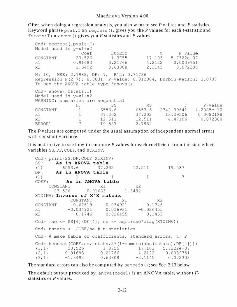
Often when doing a regression analysis, you also want to see P values and F-statistics.Keyword phrase pval:T on regress(), gives you the P values for each t-statistic andfstats:T on anova() gives you F-statistics and P values.
Cmd> regress(,pvals:T)Model used is y=x1+x2 Coef StdErr t P-ValueCONSTANT 23.526 1.3755 17.103 5.7322e-07x1 0.91683 0.21766 4.2122 0.0039751x2 -1.3492 0.63808 -2.1145 0.072308
N: 10, MSE: 2.7982, DF: 7, R^2: 0.71736Regression F(2,7): 8.8831, P-value: 0.012004, Durbin-Watson: 3.0707To see the ANOVA table type 'anova()'
Cmd> anova(,fstats:T)Model used is y=x1+x2WARNING: summaries are sequential DF SS MS F P-valueCONSTANT 1 6553.6 6553.6 2342.09641 4.2085e-10x1 1 37.202 37.202 13.29506 0.0082188x2 1 12.511 12.511 4.47106 0.072308ERROR1 7 19.587 2.7982
The P values are computed under the usual assumption of independent normal errorswith constant variance.
It is instructive to see how to compute P values for each coefficient from the side effectvariables SS, DF, COEF, and XTXINV.
Cmd> print(SS,DF,COEF,XTXINV)SS: As in ANOVA table(1) 6553.6 37.202 12.511 19.587DF: As in ANOVA table(1) 1 1 1 7COEF: As in ANOVA table CONSTANT x1 x2 23.526 0.91683 -1.3492XTXINV: Inverse of X'X matrix CONSTANT x1 x2CONSTANT 0.67619 -0.034921 -0.1746x1 -0.034921 0.016931 -0.026455x2 -0.1746 -0.026455 0.1455
Cmd> mse <- SS[4]/DF[4]; se <- sqrt(mse*diag(XTXINV))
Cmd> tstats <- COEF/se # t-statistics
Cmd> # make table of coefficients, standard errors, t, P
Cmd> hconcat(COEF,se,tstats,2*(1-cumstu(abs(tstats),DF[4])))(1,1) 23.526 1.3755 17.103 5.7322e-07(2,1) 0.91683 0.21766 4.2122 0.0039751(3,1) -1.3492 0.63808 -2.1145 0.072308
The standard errors can also be computed by secoefs(); see Sec. 3.13 below.
The default output produced by anova(Model) is an ANOVA table, without F-statistics or P values.
3-12
MacAnova Version 4.06
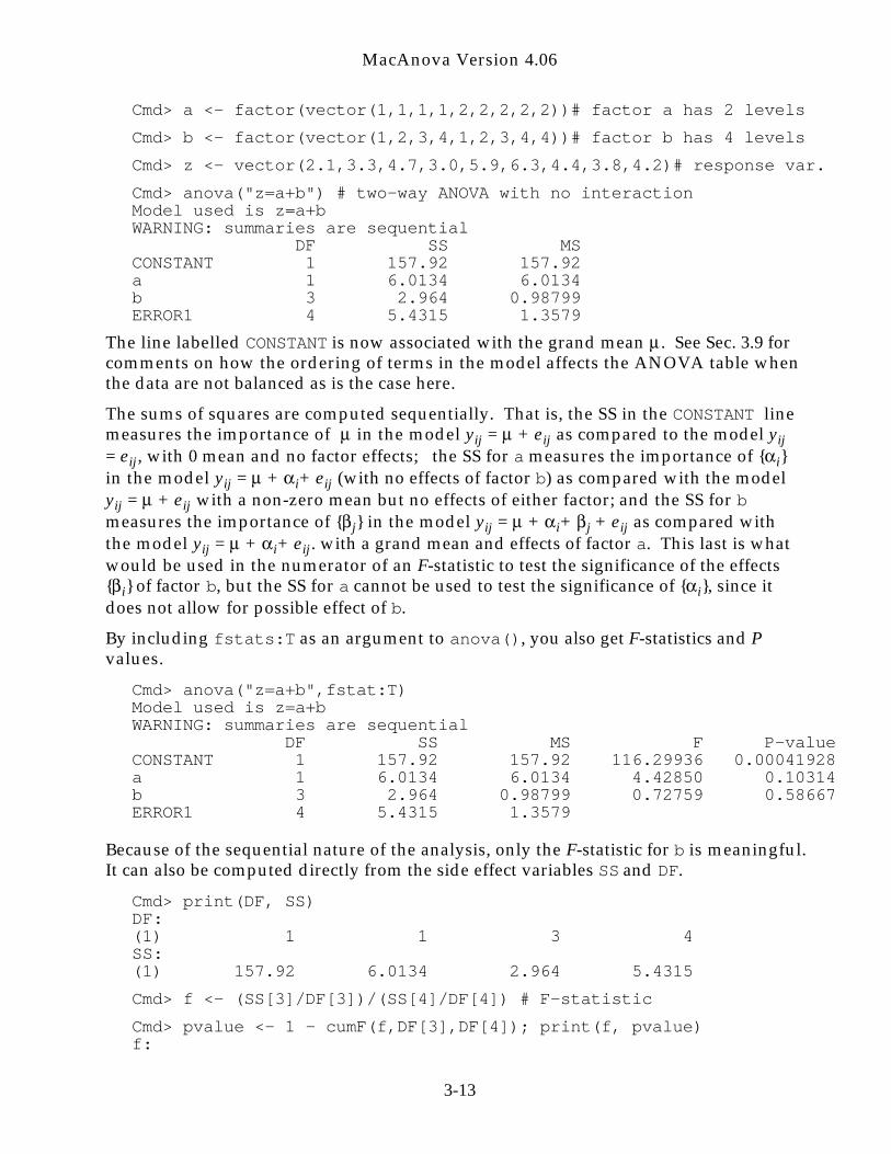
Cmd> a <- factor(vector(1,1,1,1,2,2,2,2,2))# factor a has 2 levels
Cmd> b <- factor(vector(1,2,3,4,1,2,3,4,4))# factor b has 4 levels
Cmd> z <- vector(2.1,3.3,4.7,3.0,5.9,6.3,4.4,3.8,4.2)# response var.
Cmd> anova("z=a+b") # two-way ANOVA with no interactionModel used is z=a+bWARNING: summaries are sequential DF SS MSCONSTANT 1 157.92 157.92a 1 6.0134 6.0134b 3 2.964 0.98799ERROR1 4 5.4315 1.3579
The line labelled CONSTANT is now associated with the grand mean . See Sec. 3.9 forcomments on how the ordering of terms in the model affects the ANOVA table whenthe data are not balanced as is the case here.
The sums of squares are computed sequentially. That is, the SS in the CONSTANT linemeasures the importance of in the model yij = + e ij as compared to the model yij= e ij , with 0 mean and no factor effects; the SS for a measures the importance of { i}in the model yij = + i+ e ij (with no effects of factor b) as compared with the modelyij = + e ij with a non-zero mean but no effects of either factor; and the SS for bmeasures the importance of { j} in the model yij = + i+ j + e ij as compared withthe model yij = + i+ e ij . with a grand mean and effects of factor a. This last is whatwould be used in the numerator of an F-statistic to test the significance of the effects{ i} of factor b, but the SS for a cannot be used to test the significance of { i}, since itdoes not allow for possible effect of b.
By including fstats:T as an argument to anova(), you also get F-statistics and Pvalues.
Cmd> anova("z=a+b",fstat:T)Model used is z=a+bWARNING: summaries are sequential DF SS MS F P-valueCONSTANT 1 157.92 157.92 116.29936 0.00041928a 1 6.0134 6.0134 4.42850 0.10314b 3 2.964 0.98799 0.72759 0.58667ERROR1 4 5.4315 1.3579
Because of the sequential nature of the analysis, only the F-statistic for b is meaningful.It can also be computed directly from the side effect variables SS and DF.
Cmd> print(DF, SS)DF:(1) 1 1 3 4SS:(1) 157.92 6.0134 2.964 5.4315
Cmd> f <- (SS[3]/DF[3])/(SS[4]/DF[4]) # F-statistic
Cmd> pvalue <- 1 - cumF(f,DF[3],DF[4]); print(f, pvalue)f:
3-13
MacAnova Version 4.06
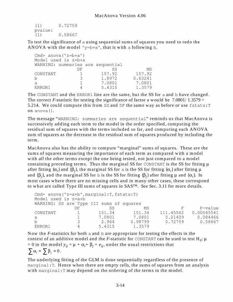
(1) 0.72759pvalue:(1) 0.58667
To test the significance of a using sequential sums of squares you need to redo theANOVA with the model "y=b+a", that is with a following b.
Cmd> anova("z=b+a")Model used is z=b+aWARNING: summaries are sequential DF SS MSCONSTANT 1 157.92 157.92b 3 1.8972 0.63241a 1 7.0801 7.0801ERROR1 4 5.4315 1.3579
The CONSTANT and the ERROR1 line are the same, but the SS for a and b have changed.The correct F-statistic for testing the significance of factor a would be 7.0801/1.3579 =5.214. We could compute this from SS and DF the same way as before or use fstats:Ton anova().
The message “WARNING: summaries are sequential” reminds us that MacAnova issuccessively adding each term to the model in the order specified, computing theresidual sum of squares with the terms included so far, and computing each ANOVAsum of squares as the decrease in the residual sum of squares produced by including theterm.
MacAnova also has the ability to compute “marginal” sums of squares. These are thesums of squares measuring the importance of each term as compared with a modelwith all the other terms except the one being tested, not just compared to a modelcontaining preceding terms. Thus the marginal SS for CONSTANT is the SS for fitting after fitting { i} and { j}, the marginal SS for a is the SS for fitting { i} after fitting and { j}, and the marginal SS for b is the SS for fitting { j} after fitting and { i}. Inmost cases where there are no missing cells and in many other cases, these correspondto what are called Type III sums of squares in SAS™. See Sec. 3.11 for more details.
Cmd> anova("z=a+b",marginal:T,fstats:T)Model used is z=a+bWARNING: SS are Type III sums of squares DF SS MS F P-valueCONSTANT 1 151.34 151.34 111.45562 0.00045541a 1 7.0801 7.0801 5.21409 0.084466b 3 2.964 0.98799 0.72759 0.58667ERROR1 4 5.4315 1.3579
Now the F-statistics for both a and b are appropriate for testing the effects in thecontext of an additive model and the F-statistic for CONSTANT can be used to test H0: = 0 in the model yij = + i+ j + e ij , under the usual restrictions that
i = j = 0∑∑ .
The underlying fitting of the GLM is done sequentially regardless of the presence ofmarginal:T. Hence when there are empty cells, the sums of squares from an analysiswith marginal:T may depend on the ordering of the terms in the model.
3-14

MacAnova Version 4.06
3.9 Balanced and unbalanced data A data set is balanced for a given model if (a) themodel contains only factors, and (b) for each pair of simple terms in the model (afterexpanding “*”, “/”, “/*” and “^”), all combinations of levels of factors that appear inone term with levels of factors that appear in the other term occur equally often in thedata set. In particular, when a design is a main effect design, that is one with nointeractions, all levels of each combination of two factors occurs equally often. A dataset is completely balanced for a model when all combinations of levels of factorsin the model occur equally often. This implies the the data set is balanced for anymodel involving only these factors, with or without interactions.
The ANOVA data in the example in the Sec. 3.8 is not balanced for the model "y = a +b" since there is only 1 observation when both factors a and b are at level 2, while thereare 2 observations at all other combinations of the factors.
Balance is important because, when it is present, the order of terms in a modelspecification has much less effect on the values of the computed sums of squares. Forexample, if every combination of factors a and b appears equally often in a data set sothat it is balanced for any model involving only a and b, then anova("y=a+b") andanova("y=b+a") produce the identical sums of squares for both a and b, although in adifferent order. Even for balanced data, some results may depend on the order or termsbecause of the sequential nature of the basic computations. For instance,anova("y=a.b+a") produces different sums of squares from anova("y=a+a.b").However, as long as no term follows a term in which it is “included”, the order ofterms will not affect the sums of squares when the data are balanced for the design.
When MacAnova recognizes balance of a data set for a model, anova() computes thesums of squares analogously to the usual hand method taught in many text books. Forlarge data sets this can be much faster than the method used for data sets that are notbalanced.
MacAnova recognizes balance only in a few situations. First, MacAnova neverrecognizes balance when there are any MISSING values or when any weights areprovided (see Sec. 3.23), even when the data would be balanced after deleting the caseswith MISSING data. Beyond this limitation, MacAnova recognizes only balanced maineffect only designs such as Latin squares, and completely balanced designs. You canalways tell whether Macanova recognized balance: If the message WARNING:summaries are sequential is printed, MacAnova did not consider the data to bebalanced. Even in this case, if the data are actually balanced, the values of the sums ofsquares do not depend on the order of terms.
Note that if any variate (as opposed to a factor) is in the model, the data are notbalanced. In a weighted ANOVA (Sec. 3.23) or non-least squares analysis (Chapter 4),the data are never considered to be balanced.
Any data set which is not balanced for a model is unbalanced. When this is the case,the sum of squares for any term in the model may be different for different orderings ofthe terms in the model. This was the case with unbalanced ANOVA example in Sec.3.8
As described in Sec. 3.8, when a data set is not balanced for a model, MacAnovanormally computes sequential sums of squares, where each successive SS represents
3-15
MacAnova Version 4.06
the improvement in model fit (as measured by reduction in the residual sum ofsquares) obtained by adding the term to the model containing only the preceding terms.In terms familiar to SAS users, MacAnova computes Type I sums of squares.
As also mentioned in Sec. 3.8, using marginal:T forces the computation of marginalsums of squares for which the SS for each term is intended to measure the contributionto the fit of that term when added to all the other terms. When there are no emptycells, and sometimes when there are, these are SAS Type III sums of squares. There issome controversy as to when these SS are appropriate in models with interactions.
When there are missing cells, the marginal SS may not be identical to Type III sums ofsquares as computed by SAS. In technical terms, each marginal SS is a quadratic formin all the estimated coefficients associated with a term as they were estimatedsequentially by Gram-Schmidt orthogonalization of the X-variables in the order ofterms given in the model. When the expectations of these estimated coefficients are 0,then each SS is distributed as 2 2, assuming normality of errors and constantvariance 2 . Since the coefficients computed by coefs() (see Sec. 3.13) are linearcombinations of these estimates, the SS can be used in an F test to test the nullhypothesis that their expectations are all 0. See Section 3.11 for more details on how themarginal SS are computed.
3.10 Parametrization and degrees of freedom (advanced topic) In its computationsMacAnova uses a variant of the classical (Scheffé) parametrization of factor effects.Consider a two factor model with factors B and C which have b and c levels,respectively.
The grand mean or intercept is associated with an X-variable consisting of all 1’s.
There are b X-variables that code for B – the constant variable containing all 1’s and,for i = 1,...,b–1, variables with 1’s for the cases (rows) in group i, –1’s for the cases ingroup b, and 0’s for other groups. Note that the first of these is the same as the X-variable coding the constant term.
Similarly, there are c X-variables that code for C – a vector of all 1’s and c–1 vectors of1’s, –1’s and 0’s.
The X-variables coding for B.C interaction are the bc pairwise products of the X-variables coding for B and C. Because the set of B and C X-variables include theconstant vector, the set of products includes copies of the constant vector and of all theB and C X-variables.
In a model with 3 or more factors, the X-variables coding for three-way interactions arethree-way products and so on.
Any variate X enters directly as an X-variable, and an interaction such as B.C.X iscoded by the product of X and the bc X-variables coding for B.C.
Note that when there are factors in the model some X-variables are redundant and thefull set is not of “full rank.” For example, in the X-variables associated with the model"y=b+c", the constant X-variable not only codes for the CONSTANT term, but is alsopresent among the X-variables that code for levels of b and those that code for levels of
3-16
MacAnova Version 4.06
c. However, when an X-variable generated from a factor is obviously a duplicate ofone encountered earlier MacAnova recognizes its redundant status, and henceforthignores it.
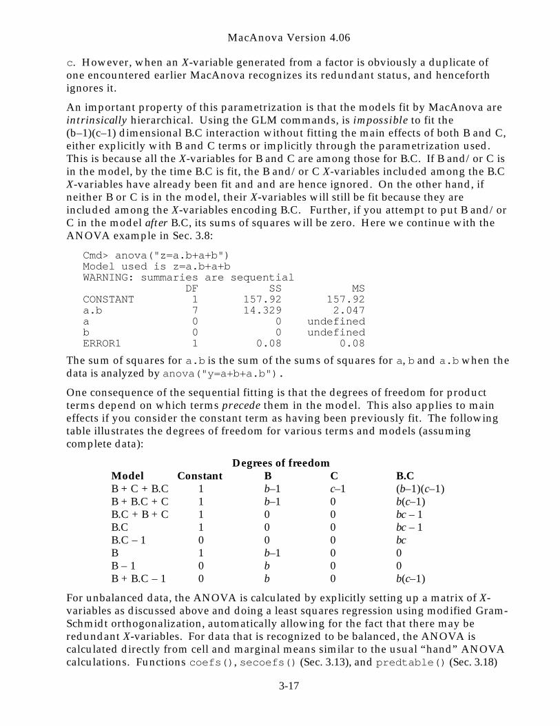
An important property of this parametrization is that the models fit by MacAnova areintrinsically hierarchical. Using the GLM commands, is impossible to fit the(b–1)(c–1) dimensional B.C interaction without fitting the main effects of both B and C,either explicitly with B and C terms or implicitly through the parametrization used.This is because all the X-variables for B and C are among those for B.C. If B and/or C isin the model, by the time B.C is fit, the B and/or C X-variables included among the B.CX-variables have already been fit and and are hence ignored. On the other hand, ifneither B or C is in the model, their X-variables will still be fit because they areincluded among the X-variables encoding B.C. Further, if you attempt to put B and/orC in the model after B.C, its sums of squares will be zero. Here we continue with theANOVA example in Sec. 3.8:
Cmd> anova("z=a.b+a+b")Model used is z=a.b+a+bWARNING: summaries are sequential DF SS MSCONSTANT 1 157.92 157.92a.b 7 14.329 2.047a 0 0 undefinedb 0 0 undefinedERROR1 1 0.08 0.08
The sum of squares for a.b is the sum of the sums of squares for a, b and a.b when thedata is analyzed by anova("y=a+b+a.b").
One consequence of the sequential fitting is that the degrees of freedom for productterms depend on which terms precede them in the model. This also applies to maineffects if you consider the constant term as having been previously fit. The followingtable illustrates the degrees of freedom for various terms and models (assumingcomplete data):
Degrees of freedomModel Constant B C B.CB + C + B.C 1 b–1 c–1 (b–1)(c–1)B + B.C + C 1 b–1 0 b(c–1)B.C + B + C 1 0 0 bc – 1B.C 1 0 0 bc – 1B.C – 1 0 0 0 bcB 1 b–1 0 0B – 1 0 b 0 0B + B.C – 1 0 b 0 b(c–1)
For unbalanced data, the ANOVA is calculated by explicitly setting up a matrix of X-variables as discussed above and doing a least squares regression using modified Gram-Schmidt orthogonalization, automatically allowing for the fact that there may beredundant X-variables. For data that is recognized to be balanced, the ANOVA iscalculated directly from cell and marginal means similar to the usual “hand” ANOVAcalculations. Functions coefs(), secoefs() (Sec. 3.13), and predtable() (Sec. 3.18)
3-17
MacAnova Version 4.06
can be used to recover the regression coefficients, estimated cell means, and treatmenteffects.
Another consequence of sequential fitting is that “marginal” sums of squares maydepend on the order of terms in the model. See Sec. 3.11
3.11 Marginal (Type III) sums of squares (advanced topic) As mentioned above, there isan alternative to computing sequential sums of square in linear models. When youuse keyword phrase marginal:T on regress(), anova() or manova(), the basiccomputational method remains the same but the side effect variable SS (and theprinted SS or SS/SP for anova() and manova()) is computed differently. Thecoefficients of the X-variables as described in Sec. 3.10 are computed sequentially in theorder of terms in the model. The SS for each term is then computed as follows.
Let ˆ
j be the vector of estimated coefficients associated with term j and let Cj be thematrix consisting of the rows and columns of (X’X)-1 corresponding to term j. Then
the marginal sum of squares for term j is SSj = ˆ j′C−1 ˆ
j . If Cj is singular because ofaliasing, the generalized inverse of Cj, obtained by setting aliased rows and columns to0 and inverting the remaining rows and columns, is used instead of Cj
-1. Assuming
independent normal errors and constant variance 2, when E[ ˆ
j ] = 0, SSj is distributedas 2
f2 where f is the degrees of freedom in the term. When there is aliasing such as
may occur when there are empty cells, ˆ
j may depend on the order of terms and henceSSj will, too. When there is no aliasing and the terms are entered in an order such thatno term comes later than another term that “contains” it (for examples, a.b.c containsa, b, c, a.b, a.c and b.c), the marginal sums of squares are the same as SAS Type IIIsums of squares.
See Sec. 3.8 for an example of the computation of marginal sums of squares.
3.12 Cell by cell statistics using tabs() and cellstats() When a, b, and c are factors (or justREAL vectors with positive integer values) and all the same length as REAL vector y,tabs(y,a,b,c) computes cell-by-cell means, variances, and counts for for each cell ofthe three-dimensional table defined by the levels of a, b and c, without assuming anyparticular model. Similarly, tabs(y,a) and tabs(y,a,b) compute statistics for thetables defined by just a and just a and b, which are one- and two-dimensional marginaltables of the 3-way table. You can include up to 31 factors in the argument list as long asthey all have have the same length. If there are any MISSING values in a cell defined bythe factors, they are not included in the count.
The output of tabs() is a structure with components mean, var, and count. Whenthere are k integer vectors a, b, ... defining the marginals, each component is a k -dimensional array (vector or matrix when k is 1 or 2). Often a, b, ... are factors createdby factor() that are used in an ANOVA model, but that need not be the case. Whenyou don’t want all three components you can specify exactly the ones you want usingkeyword phrases mean:T, var:T, or count:T. For example, tabs(y,a,b,count:T)gives only the number of non-MISSING elements in each cell defined by the levels of aand b. Keyword phrase n:T can be used instead of count:T, although the
3-18
MacAnova Version 4.06
corresponding component in the result will still be named count.
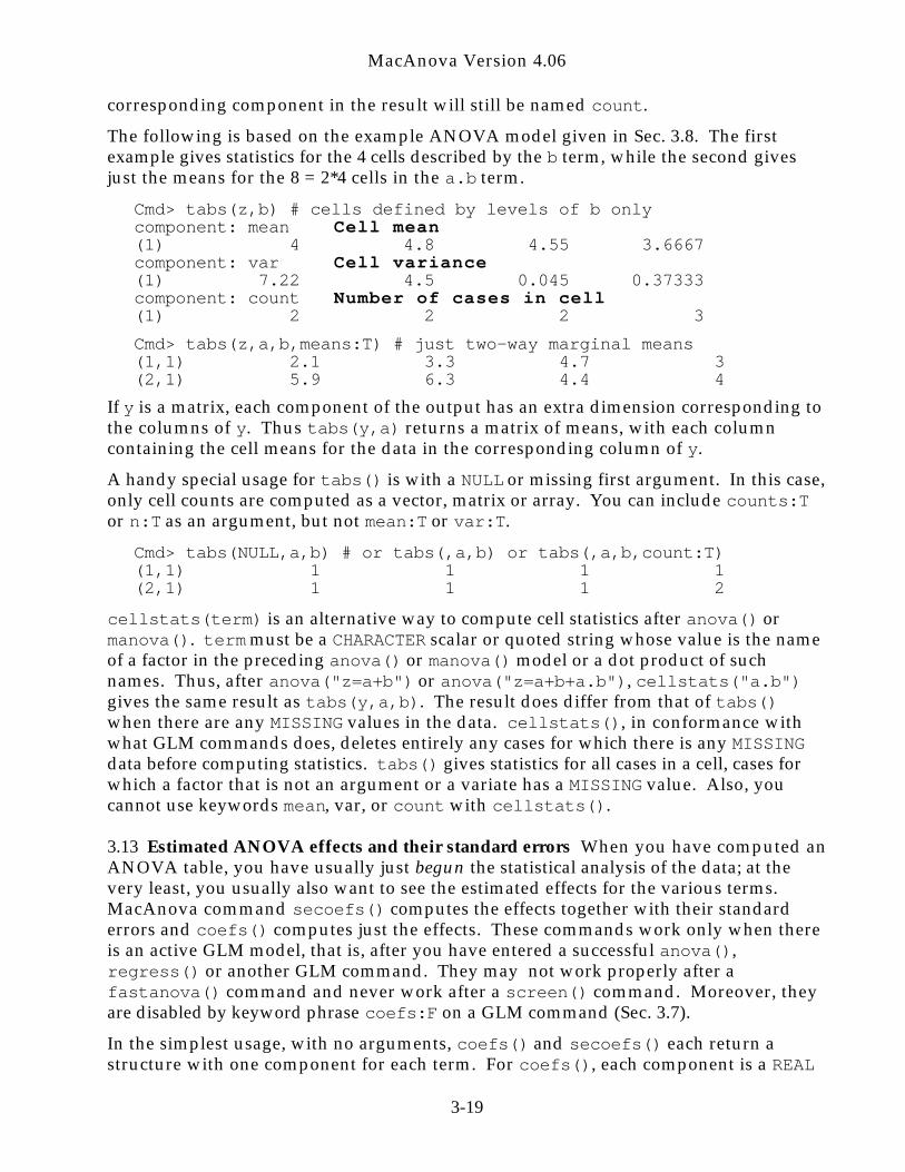
The following is based on the example ANOVA model given in Sec. 3.8. The firstexample gives statistics for the 4 cells described by the b term, while the second givesjust the means for the 8 = 2*4 cells in the a.b term.
Cmd> tabs(z,b) # cells defined by levels of b onlycomponent: mean Cell mean(1) 4 4.8 4.55 3.6667component: var Cell variance(1) 7.22 4.5 0.045 0.37333component: count Number of cases in cell(1) 2 2 2 3
Cmd> tabs(z,a,b,means:T) # just two-way marginal means(1,1) 2.1 3.3 4.7 3(2,1) 5.9 6.3 4.4 4
If y is a matrix, each component of the output has an extra dimension corresponding tothe columns of y. Thus tabs(y,a) returns a matrix of means, with each columncontaining the cell means for the data in the corresponding column of y.
A handy special usage for tabs() is with a NULL or missing first argument. In this case,only cell counts are computed as a vector, matrix or array. You can include counts:Tor n:T as an argument, but not mean:T or var:T.
Cmd> tabs(NULL,a,b) # or tabs(,a,b) or tabs(,a,b,count:T)(1,1) 1 1 1 1(2,1) 1 1 1 2
cellstats(term) is an alternative way to compute cell statistics after anova() ormanova(). term must be a CHARACTER scalar or quoted string whose value is the nameof a factor in the preceding anova() or manova() model or a dot product of suchnames. Thus, after anova("z=a+b") or anova("z=a+b+a.b"), cellstats("a.b")gives the same result as tabs(y,a,b). The result does differ from that of tabs()when there are any MISSING values in the data. cellstats(), in conformance withwhat GLM commands does, deletes entirely any cases for which there is any MISSINGdata before computing statistics. tabs() gives statistics for all cases in a cell, cases forwhich a factor that is not an argument or a variate has a MISSING value. Also, youcannot use keywords mean, var, or count with cellstats().
3.13 Estimated ANOVA effects and their standard errors When you have computed anANOVA table, you have usually just begun the statistical analysis of the data; at thevery least, you usually also want to see the estimated effects for the various terms.MacAnova command secoefs() computes the effects together with their standarderrors and coefs() computes just the effects. These commands work only when thereis an active GLM model, that is, after you have entered a successful anova(),regress() or another GLM command. They may not work properly after afastanova() command and never work after a screen() command. Moreover, theyare disabled by keyword phrase coefs:F on a GLM command (Sec. 3.7).
In the simplest usage, with no arguments, coefs() and secoefs() each return astructure with one component for each term. For coefs(), each component is a REAL
3-19
MacAnova Version 4.06
vector, array, or matrix containing the estimated coefficients for that term; forsecoefs() each component is itself a structure with components coefs and secontaining the estimated coefficients and their standard errors. If there are no degreesof freedom for error because of insufficient replication, all elements of se are MISSING.
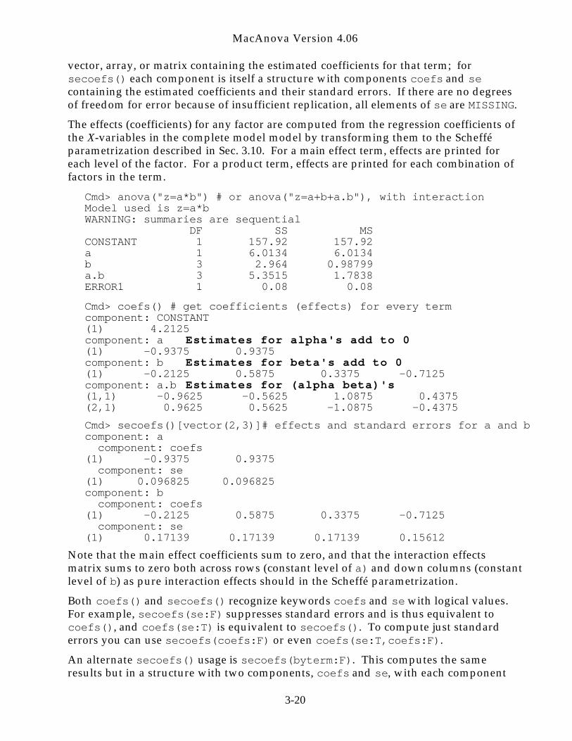
The effects (coefficients) for any factor are computed from the regression coefficients ofthe X-variables in the complete model model by transforming them to the Schefféparametrization described in Sec. 3.10. For a main effect term, effects are printed foreach level of the factor. For a product term, effects are printed for each combination offactors in the term.
Cmd> anova("z=a*b") # or anova("z=a+b+a.b"), with interactionModel used is z=a*bWARNING: summaries are sequential DF SS MSCONSTANT 1 157.92 157.92a 1 6.0134 6.0134b 3 2.964 0.98799a.b 3 5.3515 1.7838ERROR1 1 0.08 0.08
Cmd> coefs() # get coefficients (effects) for every termcomponent: CONSTANT(1) 4.2125component: a Estimates for alpha's add to 0(1) -0.9375 0.9375component: b Estimates for beta's add to 0(1) -0.2125 0.5875 0.3375 -0.7125component: a.b Estimates for (alpha beta)'s(1,1) -0.9625 -0.5625 1.0875 0.4375(2,1) 0.9625 0.5625 -1.0875 -0.4375
Cmd> secoefs()[vector(2,3)]# effects and standard errors for a and bcomponent: a component: coefs(1) -0.9375 0.9375 component: se(1) 0.096825 0.096825component: b component: coefs(1) -0.2125 0.5875 0.3375 -0.7125 component: se(1) 0.17139 0.17139 0.17139 0.15612
Note that the main effect coefficients sum to zero, and that the interaction effectsmatrix sums to zero both across rows (constant level of a) and down columns (constantlevel of b) as pure interaction effects should in the Scheffé parametrization.
Both coefs() and secoefs() recognize keywords coefs and se with logical values.For example, secoefs(se:F) suppresses standard errors and is thus equivalent tocoefs(), and coefs(se:T) is equivalent to secoefs(). To compute just standarderrors you can use secoefs(coefs:F) or even coefs(se:T,coefs:F).
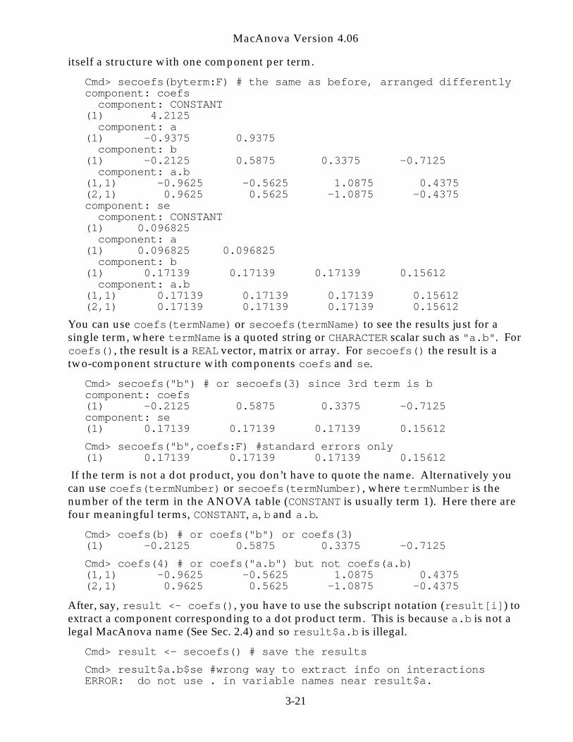
An alternate secoefs() usage is secoefs(byterm:F). This computes the sameresults but in a structure with two components, coefs and se, with each component
3-20
MacAnova Version 4.06
itself a structure with one component per term.
Cmd> secoefs(byterm:F) # the same as before, arranged differentlycomponent: coefs component: CONSTANT(1) 4.2125 component: a(1) -0.9375 0.9375 component: b(1) -0.2125 0.5875 0.3375 -0.7125 component: a.b(1,1) -0.9625 -0.5625 1.0875 0.4375(2,1) 0.9625 0.5625 -1.0875 -0.4375component: se component: CONSTANT(1) 0.096825 component: a(1) 0.096825 0.096825 component: b(1) 0.17139 0.17139 0.17139 0.15612 component: a.b(1,1) 0.17139 0.17139 0.17139 0.15612(2,1) 0.17139 0.17139 0.17139 0.15612
You can use coefs(termName) or secoefs(termName) to see the results just for asingle term, where termName is a quoted string or CHARACTER scalar such as "a.b". Forcoefs(), the result is a REAL vector, matrix or array. For secoefs() the result is atwo-component structure with components coefs and se.
Cmd> secoefs("b") # or secoefs(3) since 3rd term is bcomponent: coefs(1) -0.2125 0.5875 0.3375 -0.7125component: se(1) 0.17139 0.17139 0.17139 0.15612
Cmd> secoefs("b",coefs:F) #standard errors only(1) 0.17139 0.17139 0.17139 0.15612
If the term is not a dot product, you don’t have to quote the name. Alternatively youcan use coefs(termNumber) or secoefs(termNumber), where termNumber is thenumber of the term in the ANOVA table (CONSTANT is usually term 1). Here there arefour meaningful terms, CONSTANT, a, b and a.b.
Cmd> coefs(b) # or coefs("b") or coefs(3)(1) -0.2125 0.5875 0.3375 -0.7125
Cmd> coefs(4) # or coefs("a.b") but not coefs(a.b)(1,1) -0.9625 -0.5625 1.0875 0.4375(2,1) 0.9625 0.5625 -1.0875 -0.4375
After, say, result <- coefs(), you have to use the subscript notation (result[i]) toextract a component corresponding to a dot product term. This is because a.b is not alegal MacAnova name (See Sec. 2.4) and so result$a.b is illegal.
Cmd> result <- secoefs() # save the results
Cmd> result$a.b$se #wrong way to extract info on interactionsERROR: do not use . in variable names near result$a.
3-21
MacAnova Version 4.06
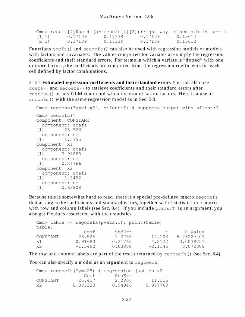
Cmd> result[4]$se # (or result[4][2]);right way, since a.b is term 4(1,1) 0.17139 0.17139 0.17139 0.15612(2,1) 0.17139 0.17139 0.17139 0.15612
Functions coefs() and secoefs() can also be used with regression models or modelswith factors and covariates. The values computed for variates are simply the regressioncoefficients and their standard errors. For terms in which a variate is “dotted” with oneor more factors, the coefficients are computed from the regression coefficients for eachcell defined by factor combinations.
3.13.1 Estimated regression coefficients and their standard errors You can also usecoefs() and secoefs() to retrieve coefficients and their standard errors afterregress() or any GLM command when the model has no factors. Here is a use ofsecoefs() with the same regression model as in Sec. 3.8.
Cmd> regress("y=x1+x2", silent:T) # suppress output with silent:T
Cmd> secoefs()component: CONSTANT component: coefs(1) 23.526 component: se(1) 1.3755component: x1 component: coefs(1) 0.91683 component: se(1) 0.21766component: x2 component: coefs(1) -1.3492 component: se(1) 0.63808
Because this is somewhat hard to read, there is a special pre-defined macro regcoefsthat arranges the coefficients and standard errors, together with t-statistics in a matrixwith row and column labels (see Sec. 8.4). If you include pvals:T as an argument, youalso get P values associated with the t-statistics.
Cmd> table <- regcoefs(pvals:T); print(table)table: Coef StdErr t P-ValueCONSTANT 23.526 1.3755 17.103 5.7322e-07x1 0.91683 0.21766 4.2122 0.0039751x2 -1.3492 0.63808 -2.1145 0.072308
The row and column labels are part of the result returned by regcoefs() (see Sec. 8.4).
You can also specify a model as an argument to regcoefs:
Cmd> regcoefs("y=x2") # regression just on x2 Coef StdErr tCONSTANT 25.417 2.2866 11.115x2 0.083333 0.94946 0.087769
3-22
MacAnova Version 4.06
When the response is multivariate (See. Sec. 3.22), regcoefs returns a structure witheach component having this form for one of the variables.
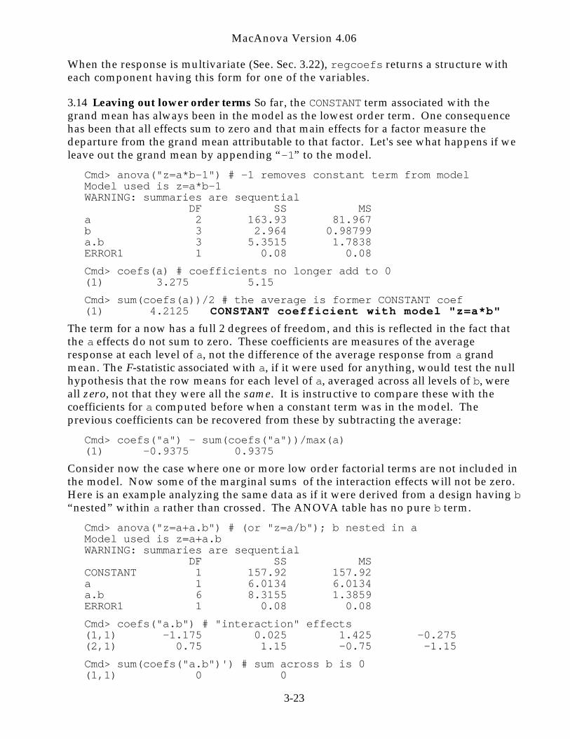
3.14 Leaving out lower order terms So far, the CONSTANT term associated with thegrand mean has always been in the model as the lowest order term. One consequencehas been that all effects sum to zero and that main effects for a factor measure thedeparture from the grand mean attributable to that factor. Let's see what happens if weleave out the grand mean by appending “-1” to the model.
Cmd> anova("z=a*b-1") # -1 removes constant term from modelModel used is z=a*b-1WARNING: summaries are sequential DF SS MSa 2 163.93 81.967b 3 2.964 0.98799a.b 3 5.3515 1.7838ERROR1 1 0.08 0.08
Cmd> coefs(a) # coefficients no longer add to 0(1) 3.275 5.15
Cmd> sum(coefs(a))/2 # the average is former CONSTANT coef(1) 4.2125 CONSTANT coefficient with model "z=a*b"
The term for a now has a full 2 degrees of freedom, and this is reflected in the fact thatthe a effects do not sum to zero. These coefficients are measures of the averageresponse at each level of a, not the difference of the average response from a grandmean. The F-statistic associated with a, if it were used for anything, would test the nullhypothesis that the row means for each level of a, averaged across all levels of b, wereall zero , not that they were all the same . It is instructive to compare these with thecoefficients for a computed before when a constant term was in the model. Theprevious coefficients can be recovered from these by subtracting the average:
Cmd> coefs("a") - sum(coefs("a"))/max(a)(1) -0.9375 0.9375
Consider now the case where one or more low order factorial terms are not included inthe model. Now some of the marginal sums of the interaction effects will not be zero.Here is an example analyzing the same data as if it were derived from a design having b“nested” within a rather than crossed. The ANOVA table has no pure b term.
Cmd> anova("z=a+a.b") # (or "z=a/b"); b nested in aModel used is z=a+a.bWARNING: summaries are sequential DF SS MSCONSTANT 1 157.92 157.92a 1 6.0134 6.0134a.b 6 8.3155 1.3859ERROR1 1 0.08 0.08
Cmd> coefs("a.b") # "interaction" effects(1,1) -1.175 0.025 1.425 -0.275(2,1) 0.75 1.15 -0.75 -1.15
Cmd> sum(coefs("a.b")') # sum across b is 0(1,1) 0 0
3-23
MacAnova Version 4.06
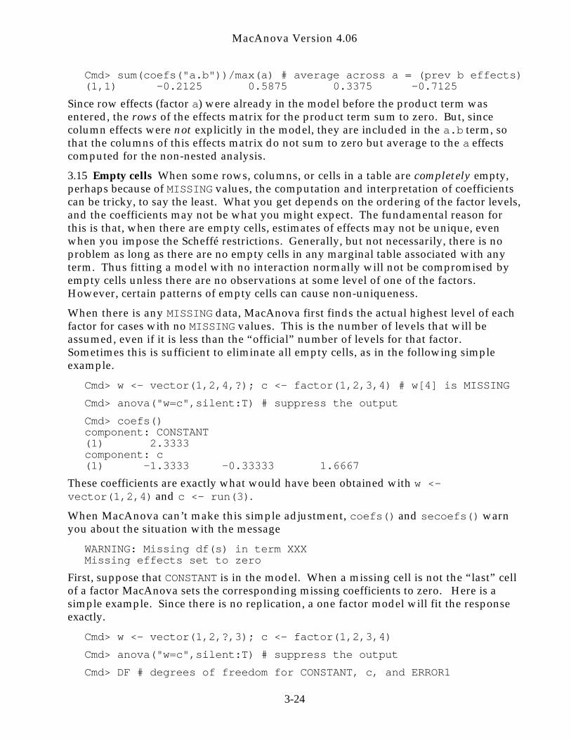
Cmd> sum(coefs("a.b"))/max(a) # average across a = (prev b effects)(1,1) -0.2125 0.5875 0.3375 -0.7125
Since row effects (factor a) were already in the model before the product term wasentered, the rows of the effects matrix for the product term sum to zero. But, sincecolumn effects were not explicitly in the model, they are included in the a.b term, sothat the columns of this effects matrix do not sum to zero but average to the a effectscomputed for the non-nested analysis.
3.15 Empty cells When some rows, columns, or cells in a table are completely empty,perhaps because of MISSING values, the computation and interpretation of coefficientscan be tricky, to say the least. What you get depends on the ordering of the factor levels,and the coefficients may not be what you might expect. The fundamental reason forthis is that, when there are empty cells, estimates of effects may not be unique, evenwhen you impose the Scheffé restrictions. Generally, but not necessarily, there is noproblem as long as there are no empty cells in any marginal table associated with anyterm. Thus fitting a model with no interaction normally will not be compromised byempty cells unless there are no observations at some level of one of the factors.However, certain patterns of empty cells can cause non-uniqueness.
When there is any MISSING data, MacAnova first finds the actual highest level of eachfactor for cases with no MISSING values. This is the number of levels that will beassumed, even if it is less than the “official” number of levels for that factor.Sometimes this is sufficient to eliminate all empty cells, as in the following simpleexample.
Cmd> w <- vector(1,2,4,?); c <- factor(1,2,3,4) # w[4] is MISSING
Cmd> anova("w=c",silent:T) # suppress the output
Cmd> coefs()component: CONSTANT(1) 2.3333component: c(1) -1.3333 -0.33333 1.6667
These coefficients are exactly what would have been obtained with w <-vector(1,2,4) and c <- run(3).
When MacAnova can’t make this simple adjustment, coefs() and secoefs() warnyou about the situation with the message
WARNING: Missing df(s) in term XXXMissing effects set to zero
First, suppose that CONSTANT is in the model. When a missing cell is not the “last” cellof a factor MacAnova sets the corresponding missing coefficients to zero. Here is asimple example. Since there is no replication, a one factor model will fit the responseexactly.
Cmd> w <- vector(1,2,?,3); c <- factor(1,2,3,4)
Cmd> anova("w=c",silent:T) # suppress the output
Cmd> DF # degrees of freedom for CONSTANT, c, and ERROR1
3-24
MacAnova Version 4.06
(1) 1 2 0
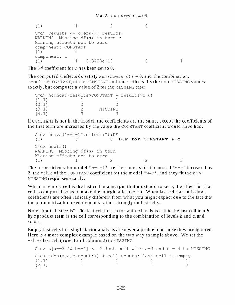
Cmd> results <- coefs(); resultsWARNING: Missing df(s) in term cMissing effects set to zerocomponent: CONSTANT(1) 2component: c(1) -1 3.3438e-19 0 1
The 3rd coefficient for c has been set to 0.
The computed c effects do satisfy sum(coefs(c)) = 0, and the combination,results$CONSTANT, of the CONSTANT and the c effects fits the non-MISSING valuesexactly, but computes a value of 2 for the MISSING case:
Cmd> hconcat(results$CONSTANT + results$c,w)(1,1) 1 1(2,1) 2 2(3,1) 2 MISSING(4,1) 3 3
If CONSTANT is not in the model, the coefficients are the same, except the coefficients ofthe first term are increased by the value the CONSTANT coefficient would have had.
Cmd> anova("w=c-1",silent:T);DF(1) 3 0 D.F for CONSTANT & c
Cmd> coefs()WARNING: Missing df(s) in term Missing effects set to zero(1) 1 2 2 3
The a coefficients for model "w=c-1" are the same as for the model "w=c" increased by2, the value of the CONSTANT coefficient for the model "w=c", and they fit the non-MISSING responses exactly.
When an empty cell is the last cell in a margin that must add to zero, the effect for thatcell is computed so as to make the margin add to zero. When last cells are missing,coefficients are often radically different from what you might expect due to the fact thatthe parametrization used depends rather strongly on last cells.
Note about “last cells”: The last cell in a factor with b levels is cell b, the last cell in a bby c product term is the cell corresponding to the combination of levels b and c, andso on.
Empty last cells in a single factor analysis are never a problem because they are ignored.Here is a more complex example based on the two way example above. We set thevalues last cell ( row 3 and column 2) to MISSING.
Cmd> z[a==2 && b==4] <- ? #set cell with a=2 and b = 4 to MISSING
Cmd> tabs(z,a,b,count:T) # cell counts; last cell is empty(1,1) 1 1 1 1(2,1) 1 1 1 0
3-25
MacAnova Version 4.06
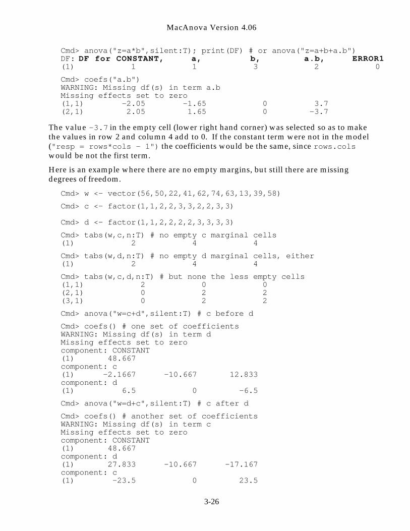
Cmd> anova("z=a*b",silent:T); print(DF) # or anova("z=a+b+a.b")DF: DF for CONSTANT, a, b, a.b, ERROR1(1) 1 1 3 2 0
Cmd> coefs("a.b")WARNING: Missing df(s) in term a.bMissing effects set to zero(1,1) -2.05 -1.65 0 3.7(2,1) 2.05 1.65 0 -3.7
The value -3.7 in the empty cell (lower right hand corner) was selected so as to makethe values in row 2 and column 4 add to 0. If the constant term were not in the model("resp = rows*cols - 1") the coefficients would be the same, since rows.colswould be not the first term.
Here is an example where there are no empty margins, but still there are missingdegrees of freedom.
Cmd> w <- vector(56,50,22,41,62,74,63,13,39,58)
Cmd> c <- factor(1,1,2,2,3,3,2,2,3,3)
Cmd> d <- factor(1,1,2,2,2,2,3,3,3,3)
Cmd> tabs(w,c,n:T) # no empty c marginal cells(1) 2 4 4
Cmd> tabs(w,d,n:T) # no empty d marginal cells, either(1) 2 4 4
Cmd> tabs(w,c,d,n:T) # but none the less empty cells(1,1) 2 0 0(2,1) 0 2 2(3,1) 0 2 2
Cmd> anova("w=c+d",silent:T) # c before d
Cmd> coefs() # one set of coefficientsWARNING: Missing df(s) in term dMissing effects set to zerocomponent: CONSTANT(1) 48.667component: c(1) -2.1667 -10.667 12.833component: d(1) 6.5 0 -6.5
Cmd> anova("w=d+c",silent:T) # c after d
Cmd> coefs() # another set of coefficientsWARNING: Missing df(s) in term cMissing effects set to zerocomponent: CONSTANT(1) 48.667component: d(1) 27.833 -10.667 -17.167component: c(1) -23.5 0 23.5
3-26
MacAnova Version 4.06
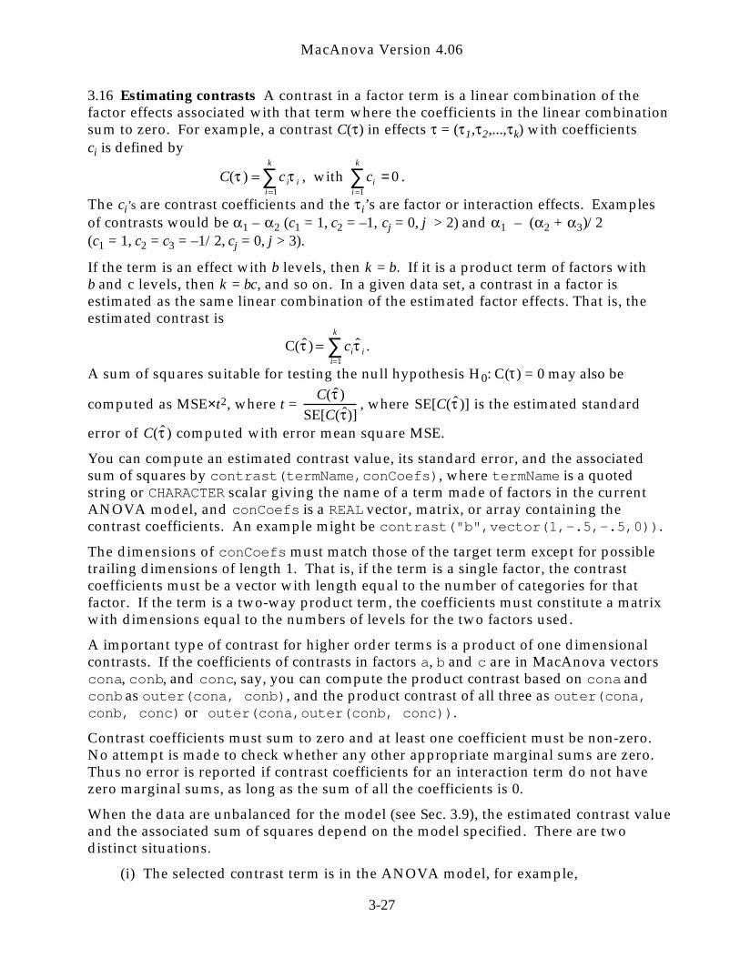
3.16 Estimating contrasts A contrast in a factor term is a linear combination of thefactor effects associated with that term where the coefficients in the linear combinationsum to zero. For example, a contrast C( ) in effects = ( 1, 2,..., k) with coefficientsci is defined by
C( ) c i ii 1
k
∑ , with ci = 0i 1
k
∑ .
The ci’s are contrast coefficients and the i’s are factor or interaction effects. Examplesof contrasts would be 1 – 2 (c1 = 1, c2 = –1, cj = 0, j > 2) and 1 – ( 2 + 3)/2(c1 = 1, c2 = c3 = –1/2, cj = 0, j > 3).
If the term is an effect with b levels, then k = b. If it is a product term of factors withb and c levels, then k = bc, and so on. In a given data set, a contrast in a factor isestimated as the same linear combination of the estimated factor effects. That is, theestimated contrast is
C( ˆ ) ciˆ
ii 1
k
∑ .
A sum of squares suitable for testing the null hypothesis H0: C(τ) = 0 may also be
computed as MSE×t2, where t = C( ˆ )
SE[C( ˆ )], where SE[C( ˆ )] is the estimated standard
error of C( ˆ ) computed with error mean square MSE.
You can compute an estimated contrast value, its standard error, and the associatedsum of squares by contrast(termName,conCoefs), where termName is a quotedstring or CHARACTER scalar giving the name of a term made of factors in the currentANOVA model, and conCoefs is a REAL vector, matrix, or array containing thecontrast coefficients. An example might be contrast("b",vector(1,-.5,-.5,0)).
The dimensions of conCoefs must match those of the target term except for possibletrailing dimensions of length 1. That is, if the term is a single factor, the contrastcoefficients must be a vector with length equal to the number of categories for thatfactor. If the term is a two-way product term, the coefficients must constitute a matrixwith dimensions equal to the numbers of levels for the two factors used.
A important type of contrast for higher order terms is a product of one dimensionalcontrasts. If the coefficients of contrasts in factors a, b and c are in MacAnova vectorscona, conb, and conc, say, you can compute the product contrast based on cona andconb as outer(cona, conb), and the product contrast of all three as outer(cona,conb, conc) or outer(cona,outer(conb, conc)).
Contrast coefficients must sum to zero and at least one coefficient must be non-zero.No attempt is made to check whether any other appropriate marginal sums are zero.Thus no error is reported if contrast coefficients for an interaction term do not havezero marginal sums, as long as the sum of all the coefficients is 0.
When the data are unbalanced for the model (see Sec. 3.9), the estimated contrast valueand the associated sum of squares depend on the model specified. There are twodistinct situations.
(i) The selected contrast term is in the ANOVA model, for example,
3-27
MacAnova Version 4.06
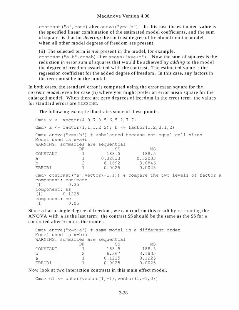
contrast("a",cona) after anova("y=a+b"). In this case the estimated value isthe specified linear combination of the estimated model coefficients, and the sumof squares is that for deleting the contrast degree of freedom from the modelwhen all other model degrees of freedom are present.
(ii) The selected term is not present in the model, for example,contrast("a.b",conab) after anova("y=a+b"). Now the sum of squares is thereduction in error sum of squares that would be achieved by adding to the modelthe degree of freedom associated with the contrast. The estimated value is theregression coefficient for the added degree of freedom. In this case, any factors inthe term must be in the model.
In both cases, the standard error is computed using the error mean square for thecurrent model , even for case (ii) where you might prefer an error mean square for theenlarged model. When there are zero degrees of freedom in the error term, the valuesfor standard errors are MISSING.
The following example illustrates some of these points.
Cmd> x <- vector(4.9,7.3,5.6,5.2,7.7)
Cmd> a <- factor(1,1,1,2,2); b <- factor(1,2,3,1,2)
Cmd> anova("x=a+b") # unbalanced because not equal cell sizesModel used is x=a+bWARNING: summaries are sequential DF SS MSCONSTANT 1 188.5 188.5a 1 0.32033 0.32033b 2 6.1692 3.0846ERROR1 1 0.0025 0.0025
Cmd> contrast("a",vector(-1,1)) # compare the two levels of factor acomponent: estimate(1) 0.35component: ss(1) 0.1225component: se(1) 0.05
Since a has a single degree of freedom, we can confirm this result by re-running theANOVA with a as the last term; the contrast SS should be the same as the SS for acomputed after b enters the model.
Cmd> anova("x=b+a") # same model in a different orderModel used is x=b+aWARNING: summaries are sequential DF SS MSCONSTANT 1 188.5 188.5b 2 6.367 3.1835a 1 0.1225 0.1225ERROR1 1 0.0025 0.0025
Now look at two interaction contrasts in this main effect model.
Cmd> c1 <- outer(vector(1,-1),vector(1,-1,0))
3-28
MacAnova Version 4.06
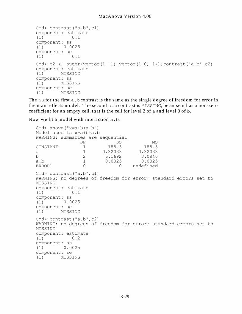
Cmd> contrast("a.b",c1)component: estimate(1) 0.1component: ss(1) 0.0025component: se(1) 0.1
Cmd> c2 <- outer(vector(1,-1),vector(1,0,-1));contrast("a.b",c2)component: estimate(1) MISSINGcomponent: ss(1) MISSINGcomponent: se(1) MISSING
The SS for the first a.b contrast is the same as the single degree of freedom for error inthe main effects model. The second a.b contrast is MISSING, because it has a non-zerocoefficient for an empty cell, that is the cell for level 2 of a and level 3 of b.
Now we fit a model with interaction a.b.
Cmd> anova("x=a+b+a.b")Model used is x=a+b+a.bWARNING: summaries are sequential DF SS MSCONSTANT 1 188.5 188.5a 1 0.32033 0.32033b 2 6.1692 3.0846a.b 1 0.0025 0.0025ERROR1 0 0 undefined
Cmd> contrast("a.b",c1)WARNING: no degrees of freedom for error; standard errors set toMISSINGcomponent: estimate(1) 0.1component: ss(1) 0.0025component: se(1) MISSING
Cmd> contrast("a.b",c2)WARNING: no degrees of freedom for error; standard errors set toMISSINGcomponent: estimate(1) 0.2component: ss(1) 0.0025component: se(1) MISSING
3-29
MacAnova Version 4.06
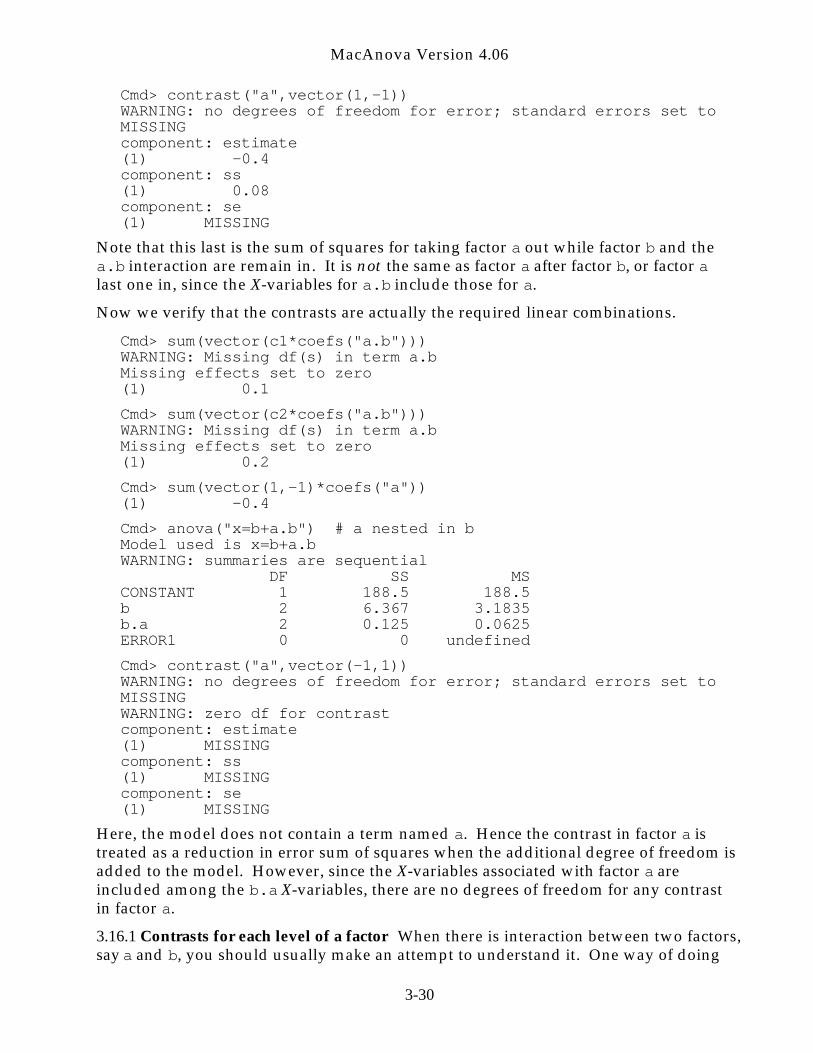
Cmd> contrast("a",vector(1,-1))WARNING: no degrees of freedom for error; standard errors set toMISSINGcomponent: estimate(1) -0.4component: ss(1) 0.08component: se(1) MISSING
Note that this last is the sum of squares for taking factor a out while factor b and thea.b interaction are remain in. It is not the same as factor a after factor b, or factor alast one in, since the X-variables for a.b include those for a.
Now we verify that the contrasts are actually the required linear combinations.
Cmd> sum(vector(c1*coefs("a.b")))WARNING: Missing df(s) in term a.bMissing effects set to zero(1) 0.1
Cmd> sum(vector(c2*coefs("a.b")))WARNING: Missing df(s) in term a.bMissing effects set to zero(1) 0.2
Cmd> sum(vector(1,-1)*coefs("a"))(1) -0.4
Cmd> anova("x=b+a.b") # a nested in bModel used is x=b+a.bWARNING: summaries are sequential DF SS MSCONSTANT 1 188.5 188.5b 2 6.367 3.1835b.a 2 0.125 0.0625ERROR1 0 0 undefined
Cmd> contrast("a",vector(-1,1))WARNING: no degrees of freedom for error; standard errors set toMISSINGWARNING: zero df for contrastcomponent: estimate(1) MISSINGcomponent: ss(1) MISSINGcomponent: se(1) MISSING
Here, the model does not contain a term named a. Hence the contrast in factor a istreated as a reduction in error sum of squares when the additional degree of freedom isadded to the model. However, since the X-variables associated with factor a areincluded among the b.a X-variables, there are no degrees of freedom for any contrastin factor a.
3.16.1 Contrasts for each level of a factor When there is interaction between two factors,say a and b, you should usually make an attempt to understand it. One way of doing
3-30
MacAnova Version 4.06
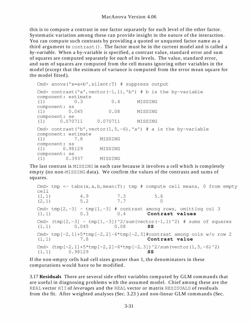
this is to compute a contrast in one factor separately for each level of the other factor.Systematic variation among these can provide insight in the nature of the interaction.You can compute such contrasts by providing a quoted or unquoted factor name as athird argument to contrast(). The factor must be in the current model and is called aby-variable. When a by-variable is specified, a contrast value, standard error and sumof squares are computed separately for each of its levels. The value, standard error,and sum of squares are computed from the cell means ignoring other variables in themodel (except that the estimate of variance is computed from the error mean square forthe model fitted).
Cmd> anova("x=a+b",silent:T) # suppress output
Cmd> contrast("a",vector(-1,1),"b") # b is the by-variablecomponent: estimate(1) 0.3 0.4 MISSINGcomponent: ss(1) 0.045 0.08 MISSINGcomponent: se(1) 0.070711 0.070711 MISSING
Cmd> contrast("b",vector(1,5,-6),"a") # a is the by-variablecomponent: estimate(1) 7.8 MISSINGcomponent: ss(1) 0.98129 MISSINGcomponent: se(1) 0.3937 MISSING
The last contrast is MISSING in each case because it involves a cell which is completelyempty (no non-MISSING data). We confirm the values of the contrasts and sums ofsquares.
Cmd> tmp <- tabs(x,a,b,mean:T); tmp # compute cell means, 0 from emptycell(1,1) 4.9 7.3 5.6(2,1) 5.2 7.7 0
Cmd> tmp[2,-3] - tmp[1,-3] # contrast among rows, omitting col 3(1,1) 0.3 0.4 Contrast values
Cmd> (tmp[2,-3] - tmp[1,-3])^2/sum(vector(-1,1)^2) # sums of squares(1,1) 0.045 0.08 SS
Cmd> tmp[-2,1]+5*tmp[-2,2]-6*tmp[-2,3]#contrast among cols w/o row 2(1,1) 7.8 Contrast value
Cmd> (tmp[-2,1]+5*tmp[-2,2]-6*tmp[-2,3])^2/sum(vector(1,5,-6)^2)(1,1) 0.98129 SS
If the non-empty cells had cell sizes greater than 1, the denominators in thesecomputations would have to be modified.
3.17 Residuals There are several side effect variables computed by GLM commands thatare useful in diagnosing problems with the assumed model. Chief among these are theREAL vector HII of leverages and the REAL vector or matrix RESIDUALS of residualsfrom the fit. After weighted analyses (Sec. 3.23 ) and non-linear GLM commands (Sec.
3-31
MacAnova Version 4.06
4.2.4, 4.2.5, 4.2.6, 4.3), RESIDUALS is still computed, but its role in diagnostic proceduresis taken by WTDRESIDUALS.
RESIDUALS contains the residuals Yi − ˆ Y i where ˆ Y i is the estimated predictable part of
the response variable for case i. RESIDUALS is usually a vector but may be a matrixafter manova(). After a weighted regression, ANOVA or MANOVA, row i of
WTDRESIDUALS is Wi (Yi − ˆ Y i) where W i is the weight for case i..
HII is a vector containing the diagonal elements of X( ′ X X)−1 ′ X , the so called hatmatrix, where X is the matrix of all the non-redundant X-variables. You cancompute the standard errors of fitted values by sqrt(HII*mse), the standard errors ofprediction by sqrt((1 + HII)*mse), and the estimated standard deviations ofestimated residuals by sqrt((1 - HII)*mse). Here mse is the mean square errorcomputed as the error sum of square divided by the error degrees of freedom. After aweighted analysis, HII consists of the diagonal elements of X( ′ X WX)−1 ′ X W , where W isthe diagonal matrix of weights.
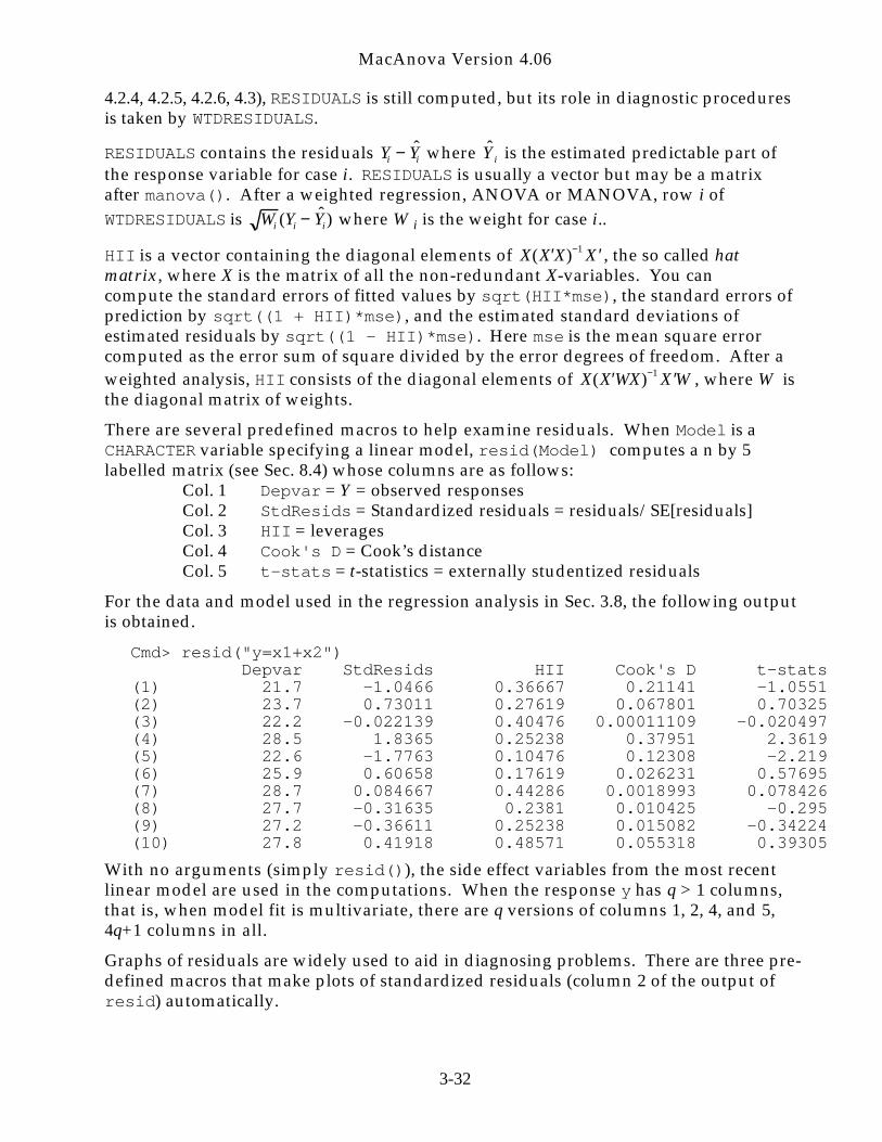
There are several predefined macros to help examine residuals. When Model is aCHARACTER variable specifying a linear model, resid(Model) computes a n by 5labelled matrix (see Sec. 8.4) whose columns are as follows:
Col. 1 Depvar = Y = observed responsesCol. 2 StdResids = Standardized residuals = residuals/SE[residuals]Col. 3 HII = leveragesCol. 4 Cook's D = Cook’s distanceCol. 5 t-stats = t-statistics = externally studentized residuals
For the data and model used in the regression analysis in Sec. 3.8, the following outputis obtained.
Cmd> resid("y=x1+x2") Depvar StdResids HII Cook's D t-stats(1) 21.7 -1.0466 0.36667 0.21141 -1.0551(2) 23.7 0.73011 0.27619 0.067801 0.70325(3) 22.2 -0.022139 0.40476 0.00011109 -0.020497(4) 28.5 1.8365 0.25238 0.37951 2.3619(5) 22.6 -1.7763 0.10476 0.12308 -2.219(6) 25.9 0.60658 0.17619 0.026231 0.57695(7) 28.7 0.084667 0.44286 0.0018993 0.078426(8) 27.7 -0.31635 0.2381 0.010425 -0.295(9) 27.2 -0.36611 0.25238 0.015082 -0.34224(10) 27.8 0.41918 0.48571 0.055318 0.39305
With no arguments (simply resid()), the side effect variables from the most recentlinear model are used in the computations. When the response y has q > 1 columns,that is, when model fit is multivariate, there are q versions of columns 1, 2, 4, and 5,4q+1 columns in all.
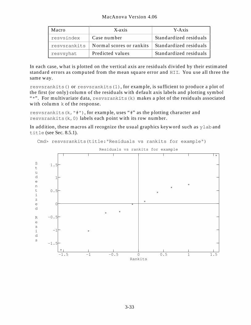
Graphs of residuals are widely used to aid in diagnosing problems. There are three pre-defined macros that make plots of standardized residuals (column 2 of the output ofresid) automatically.
3-32
MacAnova Version 4.06
Macro X-axis Y-Axis
resvsindex Case number Standardized residuals
resvsrankits Normal scores or rankits Standardized residuals
resvsyhat Predicted values Standardized residuals
In each case, what is plotted on the vertical axis are residuals divided by their estimatedstandard errors as computed from the mean square error and HII. You use all three thesame way.
resvsrankits() or resvsrankits(1), for example, is sufficient to produce a plot ofthe first (or only) column of the residuals with default axis labels and plotting symbol“*”. For multivariate data, resvsrankits(k) makes a plot of the residuals associatedwith column k of the response.
resvsrankits(k,"#"), for example, uses “#” as the plotting character andresvsrankits(k,0) labels each point with its row number.
In addition, these macros all recognize the usual graphics keyword such as ylab andtitle (see Sec. 8.5.1).
Cmd> resvsrankits(title:"Residuals vs rankits for example")
-1.5
-1
-0.5
0
0.5
1
1.5
-1.5 -1 -0.5 0 0.5 1 1.5
Residuals vs rankits for example
Rankits
Studentized Resids
*
*
*
*
*
*
*
**
*
3-33
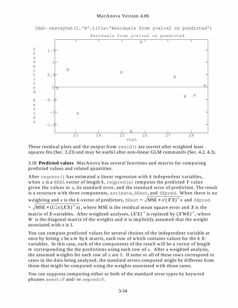
MacAnova Version 4.06
Cmd> resvsyhat(1,"R",title:"Residuals from y=x1+x2 vs predicted")
-1.5
-1
-0.5
0
0.5
1
1.5
23 24 25 26 27 28
Residuals from y=x1+x2 vs predicted
Yhat
Studentized Resids
R
R
R
R
R
R
R
RR
R
These residual plots and the output from resid() are correct after weighted leastsquares fits (Sec. 3.23) and may be useful after non-linear GLM commands (Sec. 4.2, 4.3).
3.18 Predicted values MacAnova has several functions and macros for computingpredicted values and related quantities.
After regress() has estimated a linear regression with k independent variables,when x is a REAL vector of length k , regpred(x) computes the predicted Y valuegiven the values in x, its standard error, and the standard error of prediction. The resultis a structure with three components, estimate, SEest, and SEpred. When there is no
weighting and x is the k -vector of predictors, SEest = MSE × ′ x ( ′ X X)−1 x and SEpred
= MSE × (1+ ′ x ( ′ X X)−1 x) , where MSE is the residual mean square error and X is the
matrix of X-variables. After weighted analyses, ( ′ X X)− 1 is replaced by ( ′ X WX)− 1 , whereW is the diagonal matrix of the weights and it is implicitly assumed that the weightassociated with x is 1.
You can compute predicted values for several choices of the independent variable atonce by letting x be a m by k matrix, each row of which contains values for the k X-variables. In this case, each of the components of the result will be a vector of lengthm corresponding the the predictions using each row of x. After a weighted analysis,the assumed weights for each row of x are 1. If some or all of these rows correspond tocases in the data being analyzed, the standard errors computed might be different fromthose that might be computed using the weights associated with those cases.
You can suppress computing either or both of the standard error types by keywordphrases seest:F and/or sepred:F.
3-34
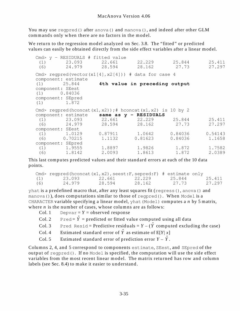
MacAnova Version 4.06
You may use regpred() after anova() and manova(), and indeed after other GLMcommands only when there are no factors in the model.
We return to the regression model analyzed on Sec. 3.8. The “fitted” or predictedvalues can easily be obtained directly from the side effect variables after a linear model.
Cmd> y - RESIDUALS # fitted value (1) 23.093 22.661 22.229 25.844 25.411 (6) 24.979 28.594 28.162 27.73 27.297
Cmd> regpred(vector(x1[4],x2[4])) # data for case 4component: estimate(1) 25.844 4th value in preceding outputcomponent: SEest(1) 0.84036component: SEpred(1) 1.872
Cmd> regpred(hconcat(x1,x2));# hconcat(x1,x2) is 10 by 2component: estimate same as y - RESIDUALS (1) 23.093 22.661 22.229 25.844 25.411 (6) 24.979 28.594 28.162 27.73 27.297component: SEest (1) 1.0129 0.87911 1.0642 0.84036 0.54143 (6) 0.70215 1.1132 0.81623 0.84036 1.1658component: SEpred (1) 1.9555 1.8897 1.9826 1.872 1.7582 (6) 1.8142 2.0093 1.8613 1.872 2.0389
This last computes predicted values and their standard errors at each of the 10 datapoints.
Cmd> regpred(hconcat(x1,x2),seest:F,sepred:F) # estimate only(1) 23.093 22.661 22.229 25.844 25.411(6) 24.979 28.594 28.162 27.73 27.297
yhat is a predefined macro that, after any least squares fit (regress(), anova() andmanova()), does computations similar to those of regpred(). When Model is aCHARACTER variable specifying a linear model, yhat(Model) computes a n by 5 matrix,where n is the number of cases, whose columns are as follows:
Col. 1 Depvar = Y = observed response
Col. 2 Pred = ̂ Y = predicted or fitted value computed using all data
Col. 3 Pred Resid = Predictive residuals = Y – ( ̂ Y computed excluding the case)
Col. 4 Estimated standard error of ̂ Y as estimate of E[Y|x]
Col. 5 Estimated standard error of prediction error Y – ̂ Y .
Columns 2, 4, and 5 correspond to components estimate, SEest, and SEpred of theoutput of regpred(). If no Model is specified, the computation will use the side effectvariables from the most recent linear model. The matrix returned has row and columnlabels (see Sec. 8.4) to make it easier to understand.
3-35
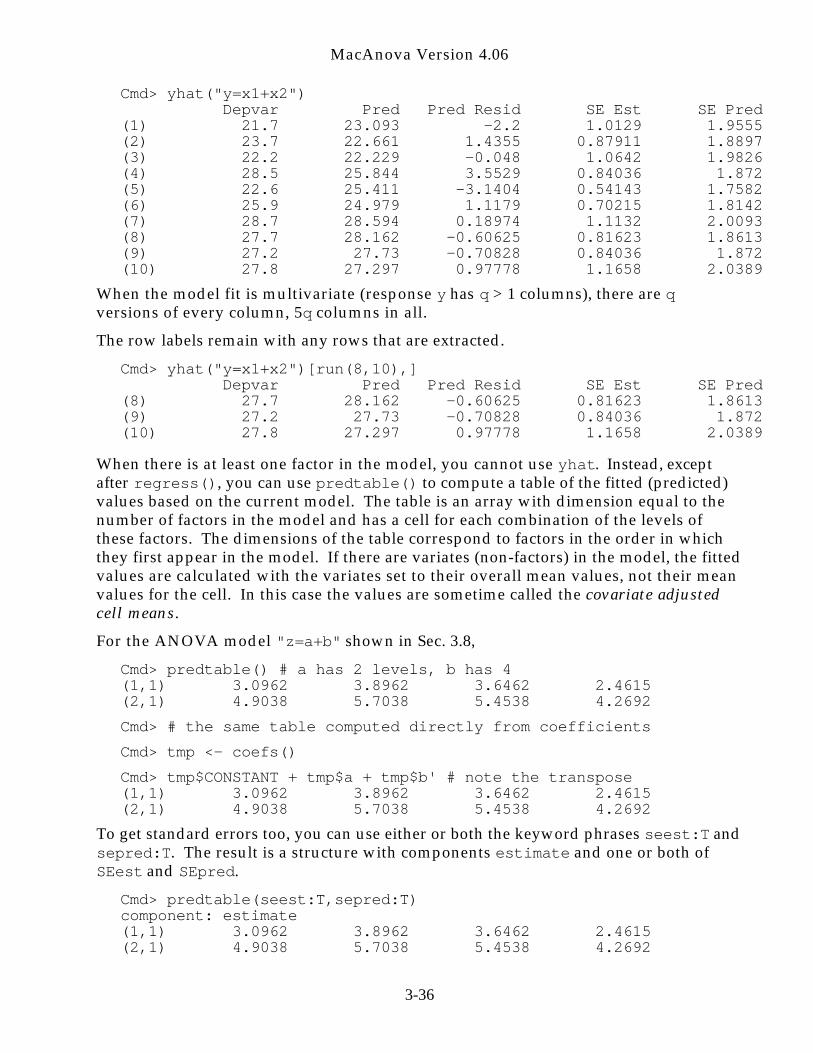
MacAnova Version 4.06
Cmd> yhat("y=x1+x2") Depvar Pred Pred Resid SE Est SE Pred(1) 21.7 23.093 -2.2 1.0129 1.9555(2) 23.7 22.661 1.4355 0.87911 1.8897(3) 22.2 22.229 -0.048 1.0642 1.9826(4) 28.5 25.844 3.5529 0.84036 1.872(5) 22.6 25.411 -3.1404 0.54143 1.7582(6) 25.9 24.979 1.1179 0.70215 1.8142(7) 28.7 28.594 0.18974 1.1132 2.0093(8) 27.7 28.162 -0.60625 0.81623 1.8613(9) 27.2 27.73 -0.70828 0.84036 1.872(10) 27.8 27.297 0.97778 1.1658 2.0389
When the model fit is multivariate (response y has q > 1 columns), there are qversions of every column, 5q columns in all.
The row labels remain with any rows that are extracted.
Cmd> yhat("y=x1+x2")[run(8,10),] Depvar Pred Pred Resid SE Est SE Pred(8) 27.7 28.162 -0.60625 0.81623 1.8613(9) 27.2 27.73 -0.70828 0.84036 1.872(10) 27.8 27.297 0.97778 1.1658 2.0389
When there is at least one factor in the model, you cannot use yhat. Instead, exceptafter regress(), you can use predtable() to compute a table of the fitted (predicted)values based on the current model. The table is an array with dimension equal to thenumber of factors in the model and has a cell for each combination of the levels ofthese factors. The dimensions of the table correspond to factors in the order in whichthey first appear in the model. If there are variates (non-factors) in the model, the fittedvalues are calculated with the variates set to their overall mean values, not their meanvalues for the cell. In this case the values are sometime called the covariate adjustedcell means .
For the ANOVA model "z=a+b" shown in Sec. 3.8,
Cmd> predtable() # a has 2 levels, b has 4(1,1) 3.0962 3.8962 3.6462 2.4615(2,1) 4.9038 5.7038 5.4538 4.2692
Cmd> # the same table computed directly from coefficients
Cmd> tmp <- coefs()
Cmd> tmp$CONSTANT + tmp$a + tmp$b' # note the transpose(1,1) 3.0962 3.8962 3.6462 2.4615(2,1) 4.9038 5.7038 5.4538 4.2692
To get standard errors too, you can use either or both the keyword phrases seest:T andsepred:T. The result is a structure with components estimate and one or both ofSEest and SEpred.
Cmd> predtable(seest:T,sepred:T)component: estimate(1,1) 3.0962 3.8962 3.6462 2.4615(2,1) 4.9038 5.7038 5.4538 4.2692
3-36
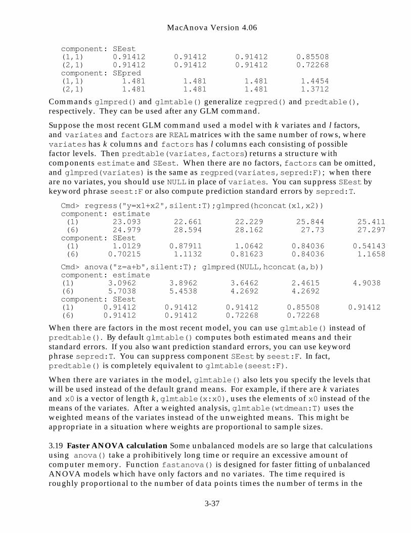
MacAnova Version 4.06
component: SEest(1,1) 0.91412 0.91412 0.91412 0.85508(2,1) 0.91412 0.91412 0.91412 0.72268component: SEpred(1,1) 1.481 1.481 1.481 1.4454(2,1) 1.481 1.481 1.481 1.3712
Commands glmpred() and glmtable() generalize regpred() and predtable(),respectively. They can be used after any GLM command.
Suppose the most recent GLM command used a model with k variates and l factors,and variates and factors are REAL matrices with the same number of rows, wherevariates has k columns and factors has l columns each consisting of possiblefactor levels. Then predtable(variates,factors) returns a structure withcomponents estimate and SEest. When there are no factors, factors can be omitted,and glmpred(variates) is the same as regpred(variates,sepred:F); when thereare no variates, you should use NULL in place of variates. You can suppress SEest bykeyword phrase seest:F or also compute prediction standard errors by sepred:T.
Cmd> regress("y=x1+x2",silent:T);glmpred(hconcat(x1,x2))component: estimate (1) 23.093 22.661 22.229 25.844 25.411 (6) 24.979 28.594 28.162 27.73 27.297component: SEest (1) 1.0129 0.87911 1.0642 0.84036 0.54143 (6) 0.70215 1.1132 0.81623 0.84036 1.1658
Cmd> anova("z=a+b",silent:T); glmpred(NULL,hconcat(a,b))component: estimate(1) 3.0962 3.8962 3.6462 2.4615 4.9038(6) 5.7038 5.4538 4.2692 4.2692component: SEest(1) 0.91412 0.91412 0.91412 0.85508 0.91412(6) 0.91412 0.91412 0.72268 0.72268
When there are factors in the most recent model, you can use glmtable() instead ofpredtable(). By default glmtable() computes both estimated means and theirstandard errors. If you also want prediction standard errors, you can use keywordphrase sepred:T. You can suppress component SEest by seest:F. In fact,predtable() is completely equivalent to glmtable(seest:F).
When there are variates in the model, glmtable() also lets you specify the levels thatwill be used instead of the default grand means. For example, if there are k variatesand x0 is a vector of length k , glmtable(x:x0), uses the elements of x0 instead of themeans of the variates. After a weighted analysis, glmtable(wtdmean:T) uses theweighted means of the variates instead of the unweighted means. This might beappropriate in a situation where weights are proportional to sample sizes. 3.19 Faster ANOVA calculation Some unbalanced models are so large that calculationsusing anova() take a prohibitively long time or require an excessive amount ofcomputer memory. Function fastanova() is designed for faster fitting of unbalancedANOVA models which have only factors and no variates. The time required isroughly proportional to the number of data points times the number of terms in the
3-37
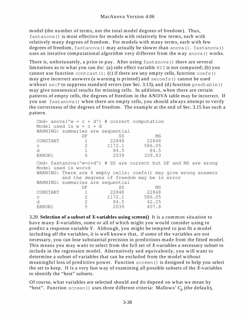
MacAnova Version 4.06
model (the number of terms, not the total model degrees of freedom). Thus,fastanova() is most effective for models with relatively few terms, each withrelatively many degrees of freedom. For models with many terms, each with fewdegrees of freedom, fastanova() may actually be slower than anova(). fastanova()uses an iterative computational algorithm very different from the way anova() works.
There is, unfortunately, a price to pay. After using fastanova() there are severallimitations as to what you can do: (a) side effect variable HII is not computed; (b) youcannot use function contrast(); (c) if there are any empty cells, function coefs()may give incorrect answers (a warning is printed) and secoefs() cannot be usedwithout se:F to suppress standard errors (see Sec. 3.13); and (d) function predtable()may give nonsensical results for missing cells. In addition, when there are certainpatterns of empty cells, the degrees of freedom in the ANOVA table may be incorrect. Ifyou use fastanova() when there are empty cells, you should always attempt to verifythe correctness of the degrees of freedom. The example at the end of Sec. 3.15 has such apattern.
Cmd> anova("w = c + d") # correct computationModel used is w = c + dWARNING: summaries are sequential DF SS MSCONSTANT 1 22848 22848c 2 1172.1 586.05d 1 84.5 84.5ERROR1 6 2039 339.83
Cmd> fastanova("w=c+d") # SS are correct but DF and MS are wrongModel used is w=c+dWARNING: There are 4 empty cells; coefs() may give wrong answers and the degrees of freedom may be in errorWARNING: summaries are sequential DF SS MSCONSTANT 1 22848 22848c 2 1172.1 586.05d 2 84.5 42.25ERROR1 5 2039 407.8
3.20 Selection of a subset of X-variables using screen() It is a common situation tohave many X-variables, some or all of which might you would consider using topredict a response variable Y. Although, you might be tempted to just fit a modelincluding all the variables, it is well known that, if some of the variables are notnecessary, you can lose substantial precision in predictions made from the fitted model.This means you may want to select from the full set of X-variables a necessary subset toinclude in the regression model. Alternatively and equivalently, you will want todetermine a subset of variables that can be excluded from the model withoutmeaningful loss of predictive power. Function screen() is designed to help you selectthe set to keep. It is a very fast way of examining all possible subsets of the X-variablesto identify the “best” subsets.
Of course, what variables are selected should and do depend on what we mean by“best”. Function screen() uses three different criteria: Mallows’ Cp (the default),
3-38
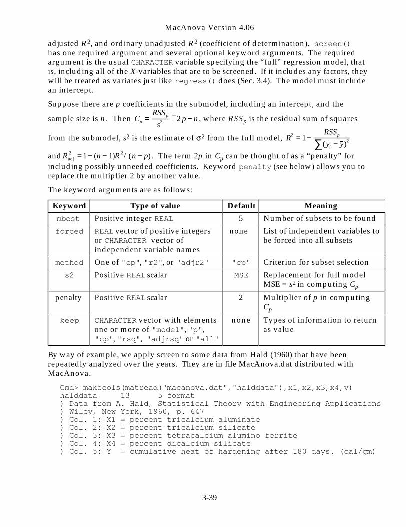
MacAnova Version 4.06
adjusted R2, and ordinary unadjusted R2 (coefficient of determination). screen()has one required argument and several optional keyword arguments. The requiredargument is the usual CHARACTER variable specifying the “full” regression model, thatis, including all of the X-variables that are to be screened. If it includes any factors, theywill be treated as variates just like regress() does (Sec. 3.4). The model must includean intercept.
Suppose there are p coefficients in the submodel, including an intercept, and the
sample size is n . Then Cp =RSSp
s2 + 2 p − n , where RSSp is the residual sum of squares
from the submodel, s2 is the estimate of 2 from the full model, R2 = 1−RSSp
(yi − y )2∑and Radj
2 = 1− (n − 1)R2/(n − p) . The term 2p in Cp can be thought of as a “penalty” forincluding possibly unneeded coefficients. Keyword penalty (see below) allows you toreplace the multiplier 2 by another value.
The keyword arguments are as follows:
Keyword Type of value Default Meaning
mbest Positive integer REAL 5 Number of subsets to be found
forced REAL vector of positive integersor CHARACTER vector ofindependent variable names
none List of independent variables tobe forced into all subsets
method One of "cp", "r2", or "adjr2" "cp" Criterion for subset selection
s2 Positive REAL scalar MSE Replacement for full modelMSE = s2 in computing Cp
penalty Positive REAL scalar 2 Multiplier of p in computingCp
keep CHARACTER vector with elementsone or more of "model", "p","cp", "rsq", "adjrsq" or "all"
none Types of information to returnas value
By way of example, we apply screen to some data from Hald (1960) that have beenrepeatedly analyzed over the years. They are in file MacAnova.dat distributed withMacAnova.
Cmd> makecols(matread("macanova.dat","halddata"),x1,x2,x3,x4,y)halddata 13 5 format) Data from A. Hald, Statistical Theory with Engineering Applications) Wiley, New York, 1960, p. 647) Col. 1: X1 = percent tricalcium aluminate) Col. 2: X2 = percent tricalcium silicate) Col. 3: X3 = percent tetracalcium alumino ferrite) Col. 4: X4 = percent dicalcium silicate) Col. 5: Y = cumulative heat of hardening after 180 days. (cal/gm)
3-39
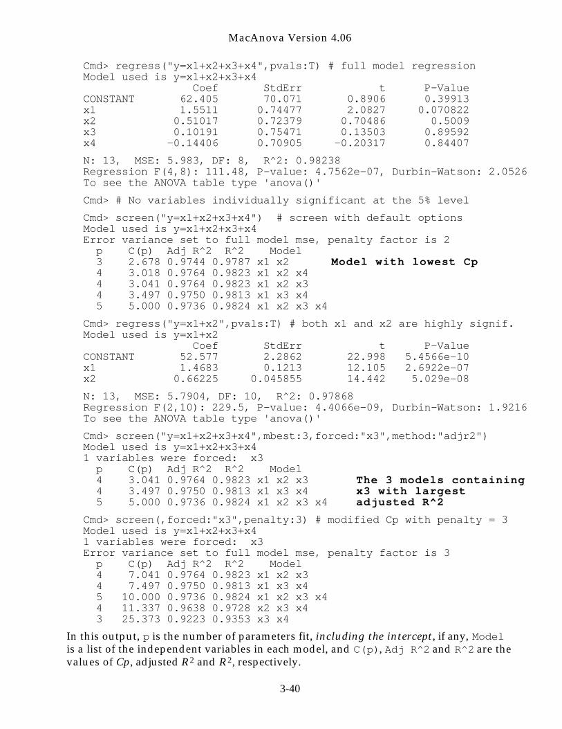
MacAnova Version 4.06
Cmd> regress("y=x1+x2+x3+x4",pvals:T) # full model regressionModel used is y=x1+x2+x3+x4 Coef StdErr t P-ValueCONSTANT 62.405 70.071 0.8906 0.39913x1 1.5511 0.74477 2.0827 0.070822x2 0.51017 0.72379 0.70486 0.5009x3 0.10191 0.75471 0.13503 0.89592x4 -0.14406 0.70905 -0.20317 0.84407
N: 13, MSE: 5.983, DF: 8, R^2: 0.98238Regression F(4,8): 111.48, P-value: 4.7562e-07, Durbin-Watson: 2.0526To see the ANOVA table type 'anova()'
Cmd> # No variables individually significant at the 5% level
Cmd> screen("y=x1+x2+x3+x4") # screen with default optionsModel used is y=x1+x2+x3+x4Error variance set to full model mse, penalty factor is 2 p C(p) Adj R^2 R^2 Model 3 2.678 0.9744 0.9787 x1 x2 Model with lowest Cp 4 3.018 0.9764 0.9823 x1 x2 x4 4 3.041 0.9764 0.9823 x1 x2 x3 4 3.497 0.9750 0.9813 x1 x3 x4 5 5.000 0.9736 0.9824 x1 x2 x3 x4
Cmd> regress("y=x1+x2",pvals:T) # both x1 and x2 are highly signif.Model used is y=x1+x2 Coef StdErr t P-ValueCONSTANT 52.577 2.2862 22.998 5.4566e-10x1 1.4683 0.1213 12.105 2.6922e-07x2 0.66225 0.045855 14.442 5.029e-08
N: 13, MSE: 5.7904, DF: 10, R^2: 0.97868Regression F(2,10): 229.5, P-value: 4.4066e-09, Durbin-Watson: 1.9216To see the ANOVA table type 'anova()'
Cmd> screen("y=x1+x2+x3+x4",mbest:3,forced:"x3",method:"adjr2")Model used is y=x1+x2+x3+x41 variables were forced: x3 p C(p) Adj R^2 R^2 Model 4 3.041 0.9764 0.9823 x1 x2 x3 The 3 models containing 4 3.497 0.9750 0.9813 x1 x3 x4 x3 with largest 5 5.000 0.9736 0.9824 x1 x2 x3 x4 adjusted R^2
Cmd> screen(,forced:"x3",penalty:3) # modified Cp with penalty = 3Model used is y=x1+x2+x3+x41 variables were forced: x3 Error variance set to full model mse, penalty factor is 3 p C(p) Adj R^2 R^2 Model 4 7.041 0.9764 0.9823 x1 x2 x3 4 7.497 0.9750 0.9813 x1 x3 x4 5 10.000 0.9736 0.9824 x1 x2 x3 x4 4 11.337 0.9638 0.9728 x2 x3 x4 3 25.373 0.9223 0.9353 x3 x4
In this output, p is the number of parameters fit, including the intercept, if any, Modelis a list of the independent variables in each model, and C(p), Adj R^2 and R^2 are thevalues of Cp , adjusted R2 and R2, respectively.
3-40
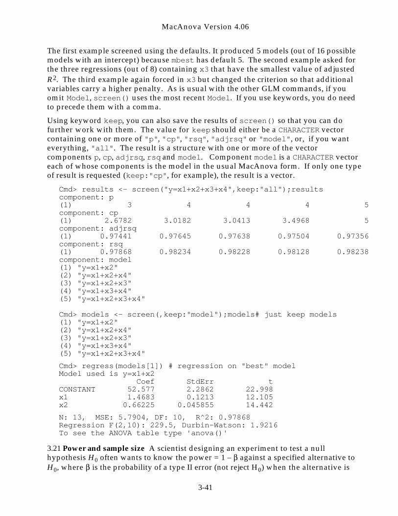
MacAnova Version 4.06
The first example screened using the defaults. It produced 5 models (out of 16 possiblemodels with an intercept) because mbest has default 5. The second example asked forthe three regressions (out of 8) containing x3 that have the smallest value of adjustedR2. The third example again forced in x3 but changed the criterion so that additionalvariables carry a higher penalty. As is usual with the other GLM commands, if youomit Model, screen() uses the most recent Model. If you use keywords, you do needto precede them with a comma.
Using keyword keep, you can also save the results of screen() so that you can dofurther work with them. The value for keep should either be a CHARACTER vectorcontaining one or more of "p", "cp", "rsq", "adjrsq" or "model", or, if you wanteverything, "all". The result is a structure with one or more of the vectorcomponents p, cp, adjrsq, rsq and model. Component model is a CHARACTER vectoreach of whose components is the model in the usual MacAnova form. If only one typeof result is requested (keep:"cp", for example), the result is a vector.
Cmd> results <- screen("y=x1+x2+x3+x4",keep:"all");resultscomponent: p(1) 3 4 4 4 5component: cp(1) 2.6782 3.0182 3.0413 3.4968 5component: adjrsq(1) 0.97441 0.97645 0.97638 0.97504 0.97356component: rsq(1) 0.97868 0.98234 0.98228 0.98128 0.98238component: model(1) "y=x1+x2"(2) "y=x1+x2+x4"(3) "y=x1+x2+x3"(4) "y=x1+x3+x4"(5) "y=x1+x2+x3+x4"
Cmd> models <- screen(,keep:"model");models# just keep models(1) "y=x1+x2"(2) "y=x1+x2+x4"(3) "y=x1+x2+x3"(4) "y=x1+x3+x4"(5) "y=x1+x2+x3+x4"
Cmd> regress(models[1]) # regression on "best" modelModel used is y=x1+x2 Coef StdErr tCONSTANT 52.577 2.2862 22.998x1 1.4683 0.1213 12.105x2 0.66225 0.045855 14.442
N: 13, MSE: 5.7904, DF: 10, R^2: 0.97868Regression F(2,10): 229.5, Durbin-Watson: 1.9216To see the ANOVA table type 'anova()'
3.21 Power and sample size A scientist designing an experiment to test a nullhypothesis H0 often wants to know the power = 1 – against a specified alternative toH0, where is the probability of a type II error (not reject H0) when the alternative is
3-41

MacAnova Version 4.06
true. Such a scientist may also want to determine the minimum sample size requiredso that the test will have power at least 1 – , where is given.
In almost every case, the power of a test depends on (i) the size of the experiment asmeasured by the number of replicates, (ii) the variance 2 of an individual observationand (iii) the extent of departure from H0 of the alternative. The last two interact intheir effect since the determining quantity is usually the departure from the nullhypothesis relative to the size of .
MacAnova provides three functions to make power and sample size computations forlinear models. power() and samplesize() are adapted to the analysis of variance ofdata from a completely randomized design (one-way ANOVA) or from a randomizedblock design (two-way ANOVA). power2() is applicable to more general designs. Theyall assume independent normal errors with constant 2.
The default usage of power() is power(noncen,ngrp,alpha,nrep), where allarguments are REAL. Argument noncen is a “noncentrality” type parameter thatspecifies the departure from the null hypothesis relative to 2. Specifically
noncen =
i2
i= 1
k
∑ / 2 ,
where k = ngrp, the number of treatments or groups; argument alpha is the size(significance or level) of the test to be used; and argument nrep is the number ofreplicates, that is, the number of units receiving each treatment. The returned value isthe power of the usual F-test for this experimental design, as computed from the non-central F-distribution.
Suppose we have 4 treatment groups, and are planning to use an F-test withsignificance level = 0.01, and we believe the noncentrality parameter is about 5. Wecompute the power for the cases when we use 5 experimental units for treatments andwhen we use 4.
Cmd> vector(power(5,4,.01,5), power(5,4,.01,4))(1) 0.8555 0.66879
We see that if we used 5 experimental units per groups the power would be .856, while4 per group would yield power of only .679. Actually the arguments to power() can bevectors, as long as all non-scalar arguments have the same length. Thus we cancompute power for several sample sizes with a single command:
Cmd> power(5,4,.01,run(4,9)) # power for sample sizes 4 through 9(1) 0.66879 0.8555 0.94585 0.98197 0.99454(6) 0.99847
Function samplesize() is a sort of inverse to power(). It has the same first threearguments, noncen, ngrp, and alpha, but its fourth argument is pwr, the requiredpower = 1 – . It returns the smallest group size giving power at least pwr. Unlikepower(), samplesize() does not accept vector arguments. Let’s find the minimumnumber of replicates required for power ≥ .80 ( ≤ .20) and power ≥ .95 ( ≤ .05) for the5 group example.
Cmd> vector(samplesize(5,4,.01,.8),samplesize(5,4,.01,.95))(1) 5 7 Sample sizes for power .80 & .95
3-42
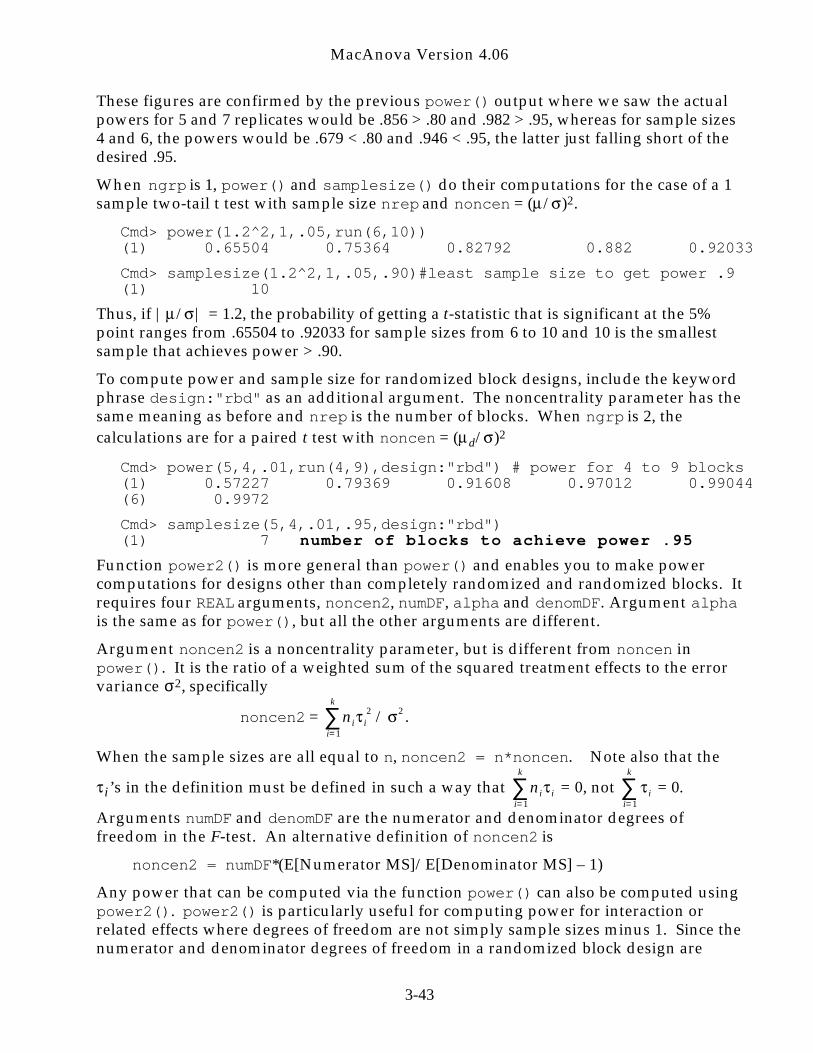
MacAnova Version 4.06
These figures are confirmed by the previous power() output where we saw the actualpowers for 5 and 7 replicates would be .856 > .80 and .982 > .95, whereas for sample sizes4 and 6, the powers would be .679 < .80 and .946 < .95, the latter just falling short of thedesired .95.
When ngrp is 1, power() and samplesize() do their computations for the case of a 1sample two-tail t test with sample size nrep and noncen = ( / )2.
Cmd> power(1.2^2,1,.05,run(6,10))(1) 0.65504 0.75364 0.82792 0.882 0.92033
Cmd> samplesize(1.2^2,1,.05,.90)#least sample size to get power .9(1) 10
Thus, if | / | = 1.2, the probability of getting a t-statistic that is significant at the 5%point ranges from .65504 to .92033 for sample sizes from 6 to 10 and 10 is the smallestsample that achieves power > .90.
To compute power and sample size for randomized block designs, include the keywordphrase design:"rbd" as an additional argument. The noncentrality parameter has thesame meaning as before and nrep is the number of blocks. When ngrp is 2, thecalculations are for a paired t test with noncen = ( d/ )2
Cmd> power(5,4,.01,run(4,9),design:"rbd") # power for 4 to 9 blocks(1) 0.57227 0.79369 0.91608 0.97012 0.99044(6) 0.9972
Cmd> samplesize(5,4,.01,.95,design:"rbd")(1) 7 number of blocks to achieve power .95
Function power2() is more general than power() and enables you to make powercomputations for designs other than completely randomized and randomized blocks. Itrequires four REAL arguments, noncen2, numDF, alpha and denomDF. Argument alphais the same as for power(), but all the other arguments are different.
Argument noncen2 is a noncentrality parameter, but is different from noncen inpower(). It is the ratio of a weighted sum of the squared treatment effects to the errorvariance σ2, specifically
noncen2 =
ni i2
i= 1
k
∑ / 2 .
When the sample sizes are all equal to n, noncen2 = n*noncen. Note also that the
i ’s in the definition must be defined in such a way that
ni ii= 1
k
∑ = 0, not
ii= 1
k
∑ = 0.
Arguments numDF and denomDF are the numerator and denominator degrees offreedom in the F-test. An alternative definition of noncen2 is
noncen2 = numDF*(E[Numerator MS]/E[Denominator MS] – 1)
Any power that can be computed via the function power() can also be computed usingpower2(). power2() is particularly useful for computing power for interaction orrelated effects where degrees of freedom are not simply sample sizes minus 1. Since thenumerator and denominator degrees of freedom in a randomized block design are
3-43
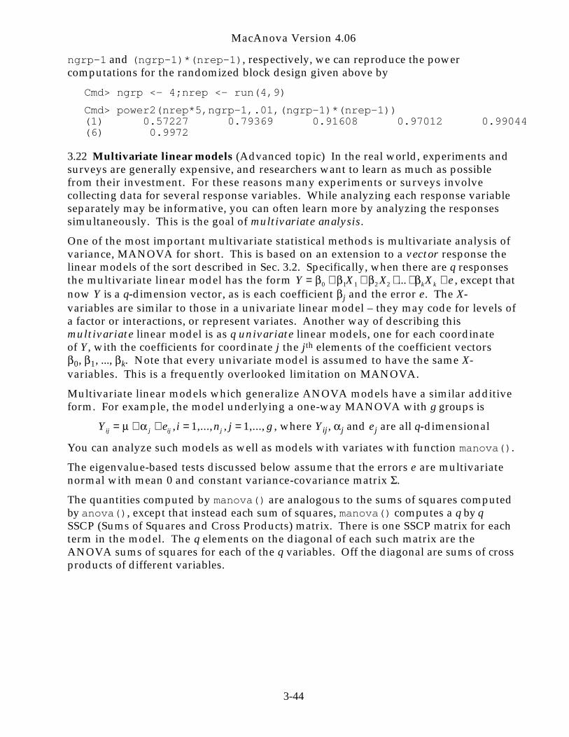
MacAnova Version 4.06
ngrp-1 and (ngrp-1)*(nrep-1), respectively, we can reproduce the powercomputations for the randomized block design given above by
Cmd> ngrp <- 4;nrep <- run(4,9)
Cmd> power2(nrep*5,ngrp-1,.01,(ngrp-1)*(nrep-1))(1) 0.57227 0.79369 0.91608 0.97012 0.99044(6) 0.9972
3.22 Multivariate linear models (Advanced topic) In the real world, experiments andsurveys are generally expensive, and researchers want to learn as much as possiblefrom their investment. For these reasons many experiments or surveys involvecollecting data for several response variables. While analyzing each response variableseparately may be informative, you can often learn more by analyzing the responsessimultaneously. This is the goal of multivariate analysis.
One of the most important multivariate statistical methods is multivariate analysis ofvariance, MANOVA for short. This is based on an extension to a vector response thelinear models of the sort described in Sec. 3.2. Specifically, when there are q responsesthe multivariate linear model has the form Y = 0 + 1X1 + 2 X2 +... + kXk + e , except thatnow Y is a q-dimension vector, as is each coefficient j and the error e . The X-variables are similar to those in a univariate linear model – they may code for levels ofa factor or interactions, or represent variates. Another way of describing thismultivariate linear model is as q univariate linear models, one for each coordinateof Y, with the coefficients for coordinate j the jth elements of the coefficient vectors
0, 1, ..., k. Note that every univariate model is assumed to have the same X-variables. This is a frequently overlooked limitation on MANOVA.
Multivariate linear models which generalize ANOVA models have a similar additiveform. For example, the model underlying a one-way MANOVA with g groups is
Yij = + j + eij ,i = 1,...,nj , j = 1,..., g , where Yij , j and e j are all q-dimensional
You can analyze such models as well as models with variates with function manova().
The eigenvalue-based tests discussed below assume that the errors e are multivariatenormal with mean 0 and constant variance-covariance matrix .
The quantities computed by manova() are analogous to the sums of squares computedby anova(), except that instead each sum of squares, manova() computes a q by qSSCP (Sums of Squares and Cross Products) matrix. There is one SSCP matrix for eachterm in the model. The q elements on the diagonal of each such matrix are theANOVA sums of squares for each of the q variables. Off the diagonal are sums of crossproducts of different variables.
3-44
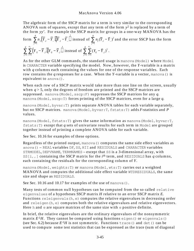
MacAnova Version 4.06
The algebraic form of the SSCP matrix for a term is very similar to the correspondingANOVA sum of squares, except that any term of the form y2 is replaced by a term ofthe form yy’. For example the SSCP matrix for groups in a one-way MANOVA has the
form
n j Y .j − Y ..( )j =1
g
∑ Y . j −Y ..( )′ instead of nj (Y . j − Y .. )2
j =1
g
∑ and the error SSCP has the form
Y ij − Y . j( ) Yij − Y . j( )′
i =1
n j
∑j =1
g
∑ instead of (Yij − Y . j )2
i =1
n j
∑j =1
g
∑ .
As for the other GLM commands, the standard usage is manova(Model) where Modelis CHARACTER variable specifying the model. Now, however, the Y-variable is a matrixwith q columns each containing the values for one of the response variables. Eachrow contains the q responses for a case. When the Y-variable is a vector, manova() isequivalent to anova().
When each row of a SSCP matrix would take more than one line on the screen, usuallywhen q > 5, only the degrees of freedom are printed and the SSCP matrices aresuppressed. manova(Model,sscp:F) suppresses the SSCP matrices for any q.manova(Model,sscp:T) forces printing of the SSCP matrices, even for a large q.
manova(Model,byvar:T) prints separate ANOVA tables for each variable separately,but no SSCP matrices. manova(Model,byvar:T,fstats:T) adds F-statistics and Pvalues.
manova(Model,fstats:T) gives the same information as manova(Model,byvar:T,fstats:T) except that q sets of univariate results for each term in Model are groupedtogether instead of printing a complete ANOVA table for each variable.
See Sec. 10.16 for examples of these options.
Regardless of the printed output, manova() computes the same side effect variables asanova() – REAL variables DF, SS, HII and RESIDUALS and CHARACTER variablesSTRMODEL, DEPVNAME, TERMNAMES – except that SS is a 3-dimensional array, withSS[i,,] containing the SSCP matrix for the ith term, and RESIDUALS has q columns,each containing the residuals for the corresponding column of Y.
manova(Model,weights:T) or manova(Model,wts:T) carries out a weightedMANOVA and computes the additional side effect variable WTDRESIDUALS, the samesize and shape as RESIDUALS.
See Sec. 10.16 and 10.17 for examples of the use of manova().
Many tests of common null hypotheses can be computed from the so called relativeeigenvalues of a hypotheses SSCP matrix H relative to an error SSCP matrix E.Functions releigenvals(h,e) computes the relative eigenvalues in decreasing orderand releigen(h,e) computes both the relative eigenvalues and relative eigenvectors.Here h and e are square matrices of the same size with e positive definite.
In brief, the relative eigenvalues are the ordinary eigenvalues of the nonsymmetricmatrix E-1H. They cannot be computed using functions eigen() or eigenvals()(see Sec. 6.2) because E-1H is not symmetric. Functions trace() and det() can beused to compute some test statistics that can be expressed as the trace (sum of diagonal
3-45
MacAnova Version 4.06
elements) of E-1H or as a determinant such as det(I + E-1H). It is beyond the scopeof this manual to summarize the tests but see Sec. 10.16 for an example where theWilks, Hotelling and Pillai statistics are computer. See Sec. 6.2.3 for details onreleigen().
After you have run manova(), you can examine the model further using the samefunctions and macros used after anova(). To extract model coefficients and/or theirstandard errors for all terms or a specified term, you can use coefs(), coefs(term),secoefs() or secoefs(term) (see Sec. 3.13, 3.13.1). The coefficients and standarderrors have an extra dimension of length q as compared to their univariatecounterparts. For example, coefs("CONSTANT") returns a 1 by q vector. You caninclude an additional positive integer argument in these functions (for example,secoefs("a.b",2)) to specify which response variable to compute coefficients for.
If there are no factors in the model, you can also use macro regcoefs (Sec. 3.13.1) toobtain coefficients and their standard errors. By default, regcoefs() returns astructure, each component of which is a matrix containing coefficients, their standarderrors and t-statistics for one column of the response. regcoefs(pvals:T) adds acolumn of P values to each component. regcoefs(byvar:T) returns a matrix with qcolumns of coefficients, q columns of standard errors, and so on.
After manova(), contrast() (see Sec. 3.16) computes a q by q SSCP matrix with 1degree of freedom instead of a SS, plus q-dimensional vectors of contrast estimates andtheir standard errors, one for each response variable. The rules for subtractive versusadditive sums of squares are exactly as for univariate ANOVA, substituting SSCP forSS. You can use predtable() or glmtable() (Sec. 3.18) to get a table of predictedvalues. Cell by cell statistics can also be computed using tabs() or cellstats().Alternatively, you can use regpred() or glmpred() to compute estimated means andtheir standard errors for specified values of the variates and or factors.
Macros resid (Sec. 3.17) and yhat (Sec. 3.18) work after manova(), except that there areq columns each of standardized residuals, Cook's distances, predicted values, and theirstandard errors. Macros resvsrankits, resvsindex, and resvsyhat also work. Forexample, simply resvsrankits() or resvsrankits(1) makes a rankit plot ofresiduals from the first column of Y, while resvsrankits(3) makes such a plot forcolumn 3.
Let B = 1 2 3 … k[ ]′, be the k by q matrix of linear model coefficients,
including the constant term, if any. Each row i’ of B consists of q coefficients for asingle X-variable in the model, one coefficient for each response variable. Thecontrasts computed by contrast() are ultimately of the form c B, where c is a 1 by krow vector that specifies a linear combination of the rows of B. Alternatively, theycan be considered as q univariate contrasts, one for each column of Y, all computedusing the same coefficients c.
3-46
MacAnova Version 4.06
In a repeated measures analysis, you may be interested in hypotheses concerningcontrasts among the columns of B, that is, among coefficients associated withdifferent response variables. Such hypotheses can be tested using matrices obtained bypre- and post-multiplying the hypothesis and error SSCP matrices by matrices whosecolumns consist of vectors of contrast coefficients. For example, in single-sample
profile analysis with model yj = + e j, j = 1, . . ., n , where 1 2 3 … q[ ] ’,
one hypothesis of interest is H0: 1 = 2 = . . . = q. This can be expressed as C = 0,
where C is the q-1 by q matrix
1 −1 0 … 0
1 0 −1 … 0
… … … … …1 0 0 … −1
. If H and E are the SSCP
matrices associated with the CONSTANT and ERROR1 terms, obtained bymanova("y=1"),then CHC’ and CEC’ are appropriate hypothesis and error matricesfor testing H0: C = 0.
3.23 Weighted analyses Weighted regression analysis, weighted ANOVA or weightedMANOVA may be appropriate when some observations have greater intrinsicvariability than others. This is the situation, for example, when you all you have areaverages of original data, plus knowledge of the sample sizes, that is, the number oforiginal data values that were included in each average. Here you would want toweight each case (average) proportional to its original sample size. In other situations,you may have estimates of the variances for each case. In that case you would want toweight inversely proportional to the variances, that is, use the reciprocals of thevariances as weights. In addition, there are a number of estimation problems that canbe solved by iterated weighted analysis, where the results from each analysis are usedto compute new weights for a new analysis, the process continuing until estimates donot change meaningfully.
You can carry out weighted analyses with weights w, where w is a non-negative REALvector, by including weights:w or wts:w as an argument after Model in regress(),anova(), or manova(). Typical usage for a regression, weighting by the reciprocal ofthe variance for each case might be regress("y=x1+x2",weights:1/sd^2), where sdis a vector of estimated standard deviations for each case.
Analyses are performed assuming that each case has variance inversely proportional toits weight; that is, the variance of case i is 2/w i. All sums of squares (and crossproducts in the case of manova()) are given on the 2 scale, that is, after multiplying
the data by wi . In fact, the computations are entirely equivalent to those done by anunweighted analysis without a constant term, when the data for the ith case, including
Yi and all Xij’s, including the constant, are multiplied by wi .
Two sets of residuals are computed and saved as side-effects for a weighted analysis.The first, RESIDUALS, is simply the vector or matrix of responses Yi minus their valuesas predicted from the model fit. The second, WTDRESIDUALS, is sqrt(w)* RESIDUALS.If the weighting has been appropriate, its elements should have approximately constant
3-47
MacAnova Version 4.06
variance 2. You should use WTDRESIDUALS rather than RESIDUALS in any outlierand influence diagnostic procedures. Macros resid, yhat, resvsindex,resvsrankits, and resvsyhat all use WTDRESIDUALS after a weighted analysis.
The REAL vector HII of leverages is also computed and is what would be obtained by an
unweighted analysis based on X-variables and responses multiplied wi .
Any cases with zero case weight are completely removed from the regression. Inparticular this means that zero case weight observations are not counted in degrees offreedom. Any MISSING weight is treated as if it were 0.
The functions coefs() (Sec. 3.13), predtable() (Sec. 3.18), and contrast() (Sec. 3.16)are available after weighted least squares operations.
Historical note: Commands wtanova(), wtmanova() and wtregress() were formerlyused for weighted analyses. They are still available but their use is deprecated.
3.24 Retrieving information about a GLM analysis (advanced topic) Although themost important results of regression, ANOVA and other GLM analyses are eitherprinted or saved as side effect variables, other results of the computation are availableonly by calling certain functions. In addition to coefs(), secoefs() (see Sec. 3.13),predtable() and regpred() (Sec. 3.18), you can use functions modelvars(),varnames(), xvariables(), xrows() and modelinfo() to retrieve various quantitiesthat were computed but neither printed nor saved in variables. For example, if yourmodel includes factors, you can obtain the actual X-variables used to code the factorlevels (see Sec. 3.10). After non-regression GLM commands such as anova(), whenXTXINV is not created as a side effect variable, you can retrieve ( ′ X X )−1. And, even if theprevious GLM command specified dependent or independent variables that weretemporary variables and hence no longer available, modelvars() can retrieve them.In addition, modelinfo() can be used to test for the existence of an active GLM model.
3.24.1 modelvars() and varnames() You use modelvars() to retrieve the variablesappearing in the preceding model. It works even when the original variables havebeen deleted. You control what you get by specifying keyword phrases or variablenumbers. modelvars(x:T) and modelvars(y:T) retrieve the variables to the rightand left of “=” in the current model specification, respectively.modelvars(factors:T) and modelvars(variates:T) retrieve the factors andvariates, respectively, on the right hand side of the model. modelvars(all:T)returns a matrix whose columns are all the variables, in the model, starting with thedependent variable (variable on left side of the model). Finally,modelvars(vector(i1,i2,...)), where i1, i2, ... are non-negative integers,retrieves variables by number, where 0 specifies the dependent variable (variable to leftof “=”).
For example, after regress("yield=x1+x2+x3+x4+x5"), both modelvars(y:T) andmodelvars(0) return the response variable yield, both modelvars(x:T) andmodelvars(variates:T) return hconcat(x1,x2,x3,x4,x5), andmodelvars(vector(2,4,5,0)) returns hconcat(x2,x4,x5,y).
After anova("y=x+a+b+a.b+c"), where x is a variate and a, b and c are factors,
3-48
MacAnova Version 4.06
modelvars(vector(1,4)) returns hconcat(x,c), modelvars(x:T) returnshconcat(x,a,b,c), modelvars(variates:T) returns x, andmodelvars(factors:T) returns hconcat(a,b,c).
You can also use modelvars() to extract the variables from a model specified by aquoted string or CHARACTER scalar as second argument. Thus, for example,modelvars(factors:T,"y=x+a+b+c+a.b") returns hconcat(a,b).
modelvars() can also be used to determine whether a model has a constant term andthe number of factors or variates in a model by using hasconst:T, nfactors:T ornvariates:T as first argument. You use nx:T to determine the total number ofvariables on the right hand side of the model. For example, when a and b are factorsand x is a variate, modelvars(hasconst:T,"y=x+a+b+a.x") returns True,modelvars(nfactors:T,"y=x+a+b+a.x") returns 2, modelvars(nvariates:T,"y=x+a+b+a.x") returns 1 and modelvars(nx:T,"y=x+a+b+a.x") returns 3.
varnames() with with no argument returns as a CHARACTER vector the names of theall the variables in the active GLM model, starting with the reponse variable. If there isno active model, the names of the variables in STRMODEL, if it exists, are returned. Themodel should not contain any variables computed “on the fly” (Sec. 3.4.1) or anypolynomial or periodic regression shortcuts (Sec. 3.4.3).
varnames(Model), where Model is a CHARACTER scalar or quoted string, returns thenames of the variables in Model. No checking is done to confirm that the model is ofthe correct form except for checking that no names have length greater than 12characters.
Cmd> regress("yield=x1+x2+x3+x4+x5", silent:T)
Cmd> varnames()(1) "yield"(2) "x1"(3) "x2"(4) "x3"(5) "x4"(6) "x5"
Cmd> varnames("y=a+b")(1) "y"(2) "a"(3) "b"
3.24.2 xvariables() You use xvariables() to compute the X-variables (see Sec. 3.2 and3.10) used by MacAnova. These do not include any redundant X-variables that arealways ignored by the GLM commands (see Sec. 3.10) although it will include any X-variables that happen to be aliased with earlier X-variables. After any GLM command,xvariables(), with no argument, returns the X-variables for the current GLM modelas a matrix with one column for each X-variable. If the model has a constant term(intercept), one of the columns, usually the first, will be all 1’s. If Model is a quotedstring or CHARACTER scalar representing a model, xvariables(Model) computes theX-variables associated with Model.
By default, if there are any MISSING values in dependent variable or any of the variates
3-49

MacAnova Version 4.06
or factors (or weights, after a weighted analysis), the corresponding row of the X-variable matrix is set to 0. If you include missing:? as an extra argument, such rowswill be set to MISSING.
It is important to recognize the difference between modelvars() and xvariables(). Ifa model contains factors, modelvars() returns the actual factors in the model, whilethe latter returns the variables encoding the factors.
Cmd> y <- vector(70.9,78.2,74.8,63.3,68.4,74.2,54.6); x <- run(7)
Cmd> a <- factor(vector(1,2,3,1,2,3,3))
Cmd> b <- factor(vector(1,1,1,2,2,2,2))
Cmd> anova("y=x+a+b")Model used is y=x+a+bWARNING: summaries are sequential DF SS MSCONSTANT 1 33520 33520x 1 143.1 143.1a 2 109.58 54.789b 1 113.1 113.1ERROR1 2 23.08 11.54
Cmd> modelvars(x:T) # retrieves hconcat(x,a,b)(1,1) 1 1 1(2,1) 2 2 1(3,1) 3 3 1(4,1) 4 1 2(5,1) 5 2 2(6,1) 6 3 2(7,1) 7 3 2
Cmd> xvariables()(1,1) 1 1 1 0 1(2,1) 1 2 0 1 1(3,1) 1 3 -1 -1 1(4,1) 1 4 1 0 -1(5,1) 1 5 0 1 -1(6,1) 1 6 -1 -1 -1(7,1) 1 7 -1 -1 -1
Column 1 of the xvariables() output encodes the constant term, column 2 is thesame as x, columns 3 and 4 encode factor a and column 5 encodes factor b.
3.24.3 xrows() xrows(Variates,Factors) computes rows of a matrix of X-variablescorresponding to variate values in Variates and factor levels in Factors, using theinformation saved by the preceding GLM command.
Let nvar be the number of variates in the model in the model and nfac be the numberof factors.
Variates should either be a REAL vector with length(Variates) = nvar , or a REALmatrix with ncols(Variates) = nvar . When there are no variates in the model, usexrows(NULL,Factors).
Factors should either be a REAL vector with length(Factors) = nfac, or a REAL
3-50
MacAnova Version 4.06
matrix with ncols(Factors) = nfac. All the elements of Factors should be positiveintegers not exceeding the maximum level for each factor. When there are no factorsin the model, use xrows(Variates,NULL) or simply xrows(Variates).
Let N v be 1 when Variates is a vector and nrows(Variates) otherwise. Similarly,let N f be 1 when Factors is a vector and nrows(Factors) otherwise. Then if N v ≠N f, you must have either N v = 1 or N f = 1 and the value of Variates or Factors isused for every row of the output.
The result is a REAL matrix with max(N v, N f) rows. Each row consists of the values ofthe X-variables (design matrix) corresponding to that row of Variates and Factors.
Cmd> xrows(6,vector(2,2)) # same model as above(1,1) 1 6 0 1 -1
After anova("y=x1+x2+a*b"), xrows(hconcat(x1,x2),hconcat(a,b)) isequivalent to xvariables().
After regress("y=x1+x2"), xrows(hconcat(x1,x2)) %*% COEF is equivalent toregpred(x0,seest:F,sepred:F).
3.24.4 modelinfo() Function modelinfo() can return a wide variety of informationabout the most recent GLM model. You specify what it should return by keywordphrases of the form what:T, where what is one of all, aliased, bitmodel, coefs,colcounts, distrib, link, parameters, scale, sigmahat, strmodel, termnames,weights, xtxinv, xvars or y.
modelinfo(all:T) returns everything. To suppress specific items with all:T, use, forexample, modelinfo(all:T,y:F,xvars:F).
When more than one item is requested, modelinfo() returns a structure withcomponents matching these keywords. Any component that is not available (forexample, sigmahat after any GLM command except robust()) is set to NULL.
You cannot use modelinfo() after fastanova(), ipf() or screen().
Normally, using modelinfo() is an error when there was no preceding GLMcommand. However, if nomodelok:T is an argument, when there is no active modelmodelinfo() returns NULL without printing an error message. Thus you can test forthe existence of an active model by
Cmd> if(isnull(modelinfo(strmodel:T,nomodelok:T))){..do something..} # see Sec. 9.4.2 for isnull()
Here is a description of what each option returns. The preceding GLM command isanova("y=x+a+b") analyzing the data in Sec. 3.24.2.
xvars:TThe matrix of X-variables associated with the active model, that is, the same as theoutput of xvariables() (Sec. 3.24.2). As with xvariables(), you can use keywordphrase missing:? to force values for cases with any MISSING data or weights to beMISSING. The default value is 0.
y:TThe dependent variable in the model (variable to the left of “=”). modelinfo(y:T) is
3-51
MacAnova Version 4.06
thus equivalent to modelvars(0) and modelvars(y:T) (Sec. 3.24.1).
weights:TA REAL vector containing the weights associated with each case. When no weightswere specified, either explicitly or implicitly, this is a vector of 1's. Otherwise it iseither the vector wts from regress(Model,weights:wts), anova(Model,weights:wts), or manova(Model,weights:wts) (Sec. 3.23), or the implicit weightsfrom the final iteration of the iterative GLM commands such as poisson(),logistic(), or robust() (Sec. 4.2, 4.3). The value for any case with MISSING data orweight is always zero.
Cmd> modelinfo(weights:T)(1) 1 1 1 1 1(6) 1 1
parameters:TThe REAL vector containing parameters for the response variable for each case. It’svalue is different from NULL only after logistic(), probit() (Sec. 4.2.4) orglmfit(model,distrib:"binomial",...) (Sec. 4.2.6) when its value is the vectoror sample sizes for each case.
coefs:TThe vector of coefficients of the X-variables in the model fitted (Sec. 3.2, 3.10).Coefficients corresponding to aliased X-variables (those that are linearly dependenton previous X-variables) are set to zero. After manova() the result is a matrix withthe same number of columns as the dependent variable. When there are factors inthe model, the coefficients will differ from the factor effects computed by coefs() andsecoefs(). You can compute the fitted values of the response bymodelinfo(xvars:T) %*% modelinfo(coefs:T).
Cmd> modelinfo(coefs:T)(1) 130.78 -16.9 -21.433 1.6667 -22.35
Cmd> coefs() # variate coefficients and factor effectscomponent: CONSTANT(1) 130.78component: x(1) -16.9component: a(1) -21.433 1.6667 19.767component: b(1) -22.35 22.35
scale:TA REAL factor or factors by which the square roots of the diagonals of ( ′ X X )−1 or
( ′ X WX )−1 may be multiplied so as to obtain estimated standard errors for theestimated coefficients returned by modelinfo(coefs:T). After iterative GLMcommands such as logistic() or poisson(), the scale value will be the defaultvalue (usually 1), unless it was changed by keyword scale on the GLM command.
After other GLM commands, including robust(), the value will be SSError /dfError ,where dferror and SSerror come from the final line of the ANOVA table. After
3-52
MacAnova Version 4.06
manova(), the value will be the vector diag[SSCPError ]/dfError .
Cmd> @s <- modelinfo(scale:T);vector(@s,@s^2) #compare with ANOVA(1) 3.3971 11.54
sigmahat:TThe robust estimate of printed after an approximate ANOVA table computed byrobust(). After any other GLM command modelinfo(sigmahat:T) returns NULL.Note that this value should not be used in computing standard errors; usemodelinfo(scale:T) instead. See above.
xtxinv:TThe matrix ( ′ X X )−1 computed from the non-aliased X-variables. The row andcolumn corresponding to any aliased X-variable is set to zero. If the previous GLMcommand specified weights either explicitly (weights:wts on anova(), regress(),or manova()) or implicitly (iterative GLM commands such as poisson() orlogistic()) the matrix computed is ( ′ X WX )−1 , where W is the diagonal matrix ofthe weights. After robust(), the matrix computed is ( ′ X X )−1, ignoring the implicitweights. You can obtain the weights by modelinfo(weights:T) (see above).
Cmd> modelinfo(xtxinv:T)(1,1) 21.75 -6 -6.5833 -0.58333 -9.5833(2,1) -6 1.6667 1.8333 0.16667 2.6667(3,1) -6.5833 1.8333 2.3333 -1.6274e-16 2.9167(4,1) -0.58333 0.16667 -1.6274e-16 0.33333 0.25(5,1) -9.5833 2.6667 2.9167 0.25 4.4167
colcount:TA vector of integers containing the numbers of X-variables as returned byxvariables() or modelinfo(xvar:T) associated with each term in the activemodel, including any aliased X-variables. You can compute the indices of first X-variable associated with each term by autoreg(1,modelinfo(colcount:T)) whichcalculates cumulative sums. When no X-variables are aliased with earlier X-variables, the value of modelinfo(colcount:T) should be the same as side effectvariables DF excluding the error degrees of freedom.
Cmd> modelinfo(colcount:T) # since no aliasing, same as DF[-5](1) 1 1 2 1
aliased:TA LOGICAL vector whose length is the number of X-variables in the model(ncols(xvariables()). The ith element is True if and only if the ith X-variable isaliased with (linearly depending on) previous X-variables. When there is no aliasingevery element should be False.
Cmd> modelinfo(aliased:T) # no aliasing in current model(1) F F F F F
distrib:TA CHARACTER scalar containing the name of the assumed distribution of thedependent variable. It has value "normal" after anova(), regress() and manova(),value "poisson" after poisson(), value "binomial" after logistic() andprobit(), value "unknown" after robust() and the value of keyword distrib afterglmfit().
3-53
MacAnova Version 4.06
Cmd> modelinfo(distrib:T)(1) "normal"
link:TA CHARACTER scalar containing the name of the transformation assumed to berequired for the dependent variable to depend linearly on the X-variables. It hasvalue "identity" after anova(), regress(), manova() and robust(), value"logit" after logistic(), value "log" after poisson(), value "probit" afterprobit(), and the value of keyword link after glmfit().
Cmd> modelinfo(link:T)(1) "identity"
strmodel:TA CHARACTER scalar containing the current model. This will normally be the same asside effect variable STRMODEL.
Cmd> modelinfo(strmodel:T)(1) "y=1+x+a+b"
bitmodel:TA REAL vector or matrix with as many rows as there are terms in the model,including the CONSTANT term, if any, but excluding the final error term. This encodesthe model in a special form. See Sec. 3.24.5 below for details.
termnames:TA CHARACTER vector that is normally identical to side effect variable TERMNAMES. Thisincludes the name of the final error term (usually "ERROR1") and hencelength(modelinfo(termnames:T))-1 is the number of terms in the model,excluding the error term.
Cmd> modelinfo(termnames:T)(1) "CONSTANT"(2) "x"(3) "a"(4) "b"(5) "ERROR1"
all:T
Cmd> result <- modelinfo(all:T); ncomps(result) # 15 components(1) 15
Cmd> compnames(result)[run(3)] # names of 1st 3 components(1) "xvars"(2) "y"(3) "parameters"
3.24.5 Decoding modelinfo(bitmodel:T) The output from modelinfo(bitmodel:T) isa vector or matrix with one row for each term in the model. Every element is aninteger between 0 and 4294967295 = 232 – 1. The bits of the binary representation of thenumber in each row encode the variates and/or factors appearing in the correspondingterm.
Let k be the number of variates and factors in the model. When 1 ≤ k ≤ 32, the result
3-54
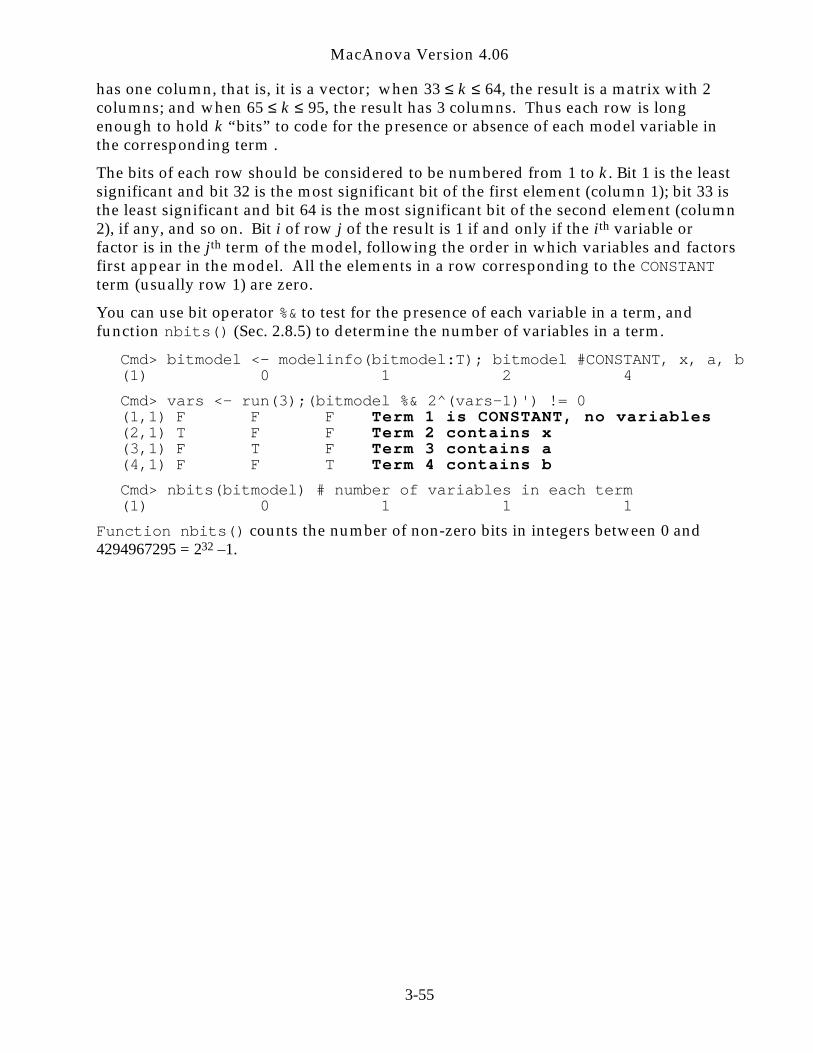
MacAnova Version 4.06
has one column, that is, it is a vector; when 33 ≤ k ≤ 64, the result is a matrix with 2columns; and when 65 ≤ k ≤ 95, the result has 3 columns. Thus each row is longenough to hold k “bits” to code for the presence or absence of each model variable inthe corresponding term .
The bits of each row should be considered to be numbered from 1 to k . Bit 1 is the leastsignificant and bit 32 is the most significant bit of the first element (column 1); bit 33 isthe least significant and bit 64 is the most significant bit of the second element (column2), if any, and so on. Bit i of row j of the result is 1 if and only if the ith variable orfactor is in the jth term of the model, following the order in which variables and factorsfirst appear in the model. All the elements in a row corresponding to the CONSTANTterm (usually row 1) are zero.
You can use bit operator %& to test for the presence of each variable in a term, andfunction nbits() (Sec. 2.8.5) to determine the number of variables in a term.
Cmd> bitmodel <- modelinfo(bitmodel:T); bitmodel #CONSTANT, x, a, b(1) 0 1 2 4
Cmd> vars <- run(3);(bitmodel %& 2^(vars-1)') != 0(1,1) F F F Term 1 is CONSTANT, no variables(2,1) T F F Term 2 contains x(3,1) F T F Term 3 contains a(4,1) F F T Term 4 contains b
Cmd> nbits(bitmodel) # number of variables in each term(1) 0 1 1 1
Function nbits() counts the number of non-zero bits in integers between 0 and4294967295 = 232 –1.
3-55