Modelling Biological Systems with Differential Equations

Rainer Breitling(R.Breitling@bio.gla.ac.uk)

Bioinformatics Research CentreFebruary 2005

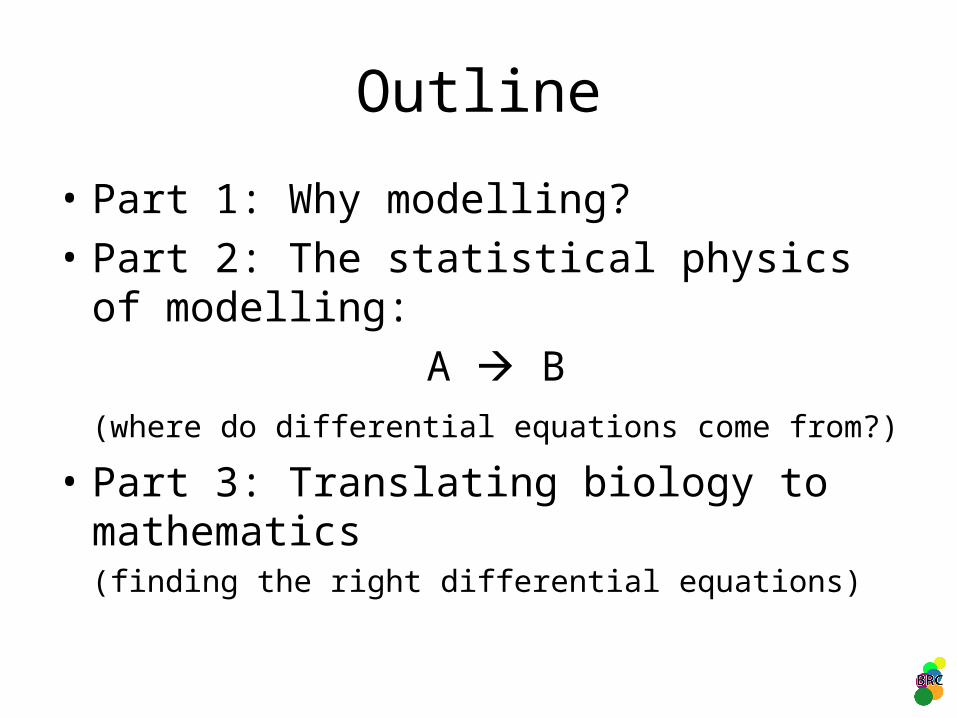
Outline

• Part 1: Why modelling?

• Part 2: The statistical physics of modelling:

A B(where do differential equations come from?)

• Part 3: Translating biology to mathematics(finding the right differential equations)

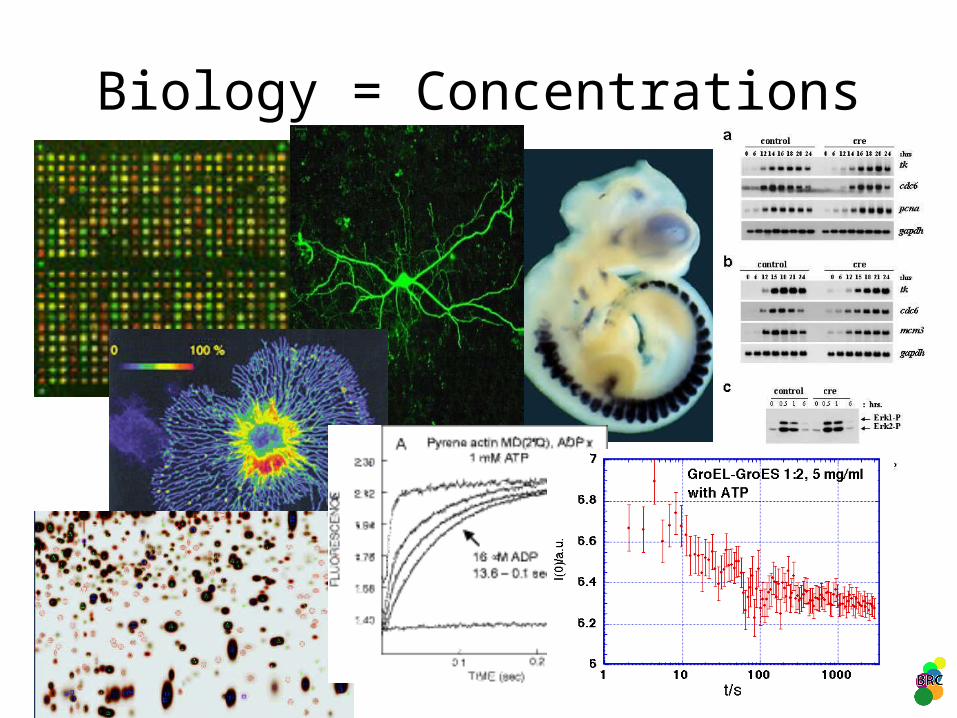
Biology = Concentrations

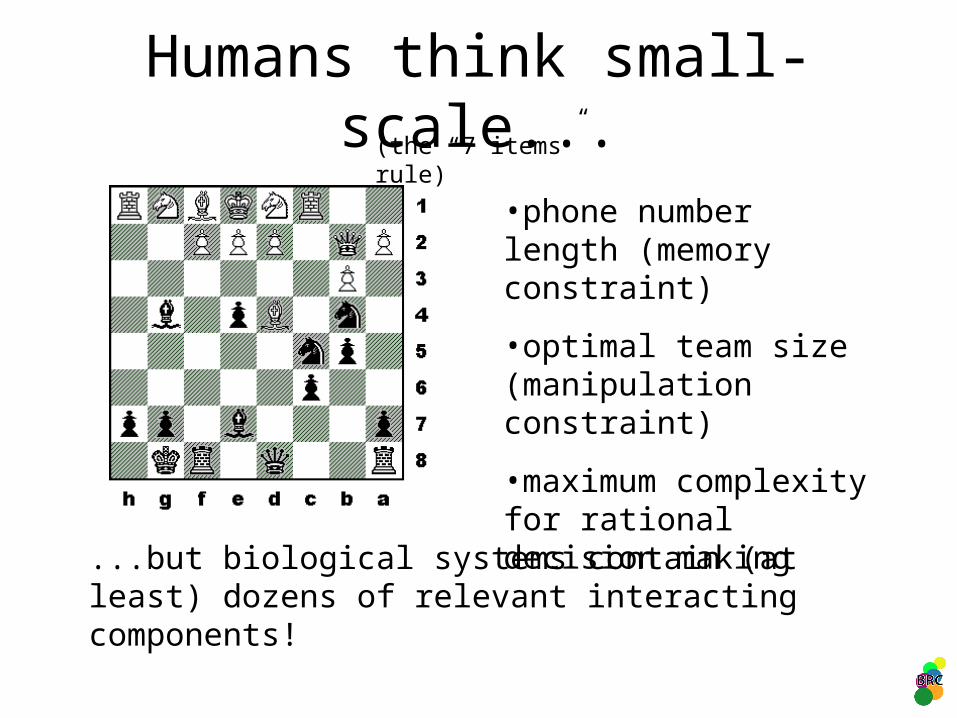
Humans think small-scale...(the “7 items” rule)

...but biological systems contain (at least) dozens of relevant interacting components!

•phone number length (memory constraint)

•optimal team size (manipulation constraint)

•maximum complexity for rational decision making

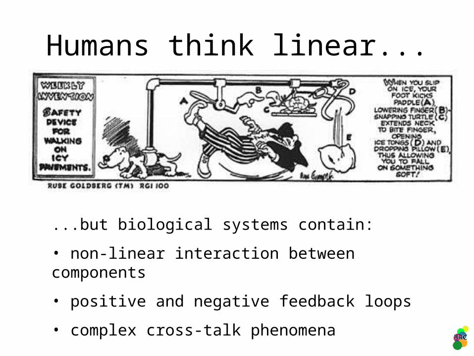
Humans think linear...

...but biological systems contain:

• non-linear interaction between components

• positive and negative feedback loops

• complex cross-talk phenomena

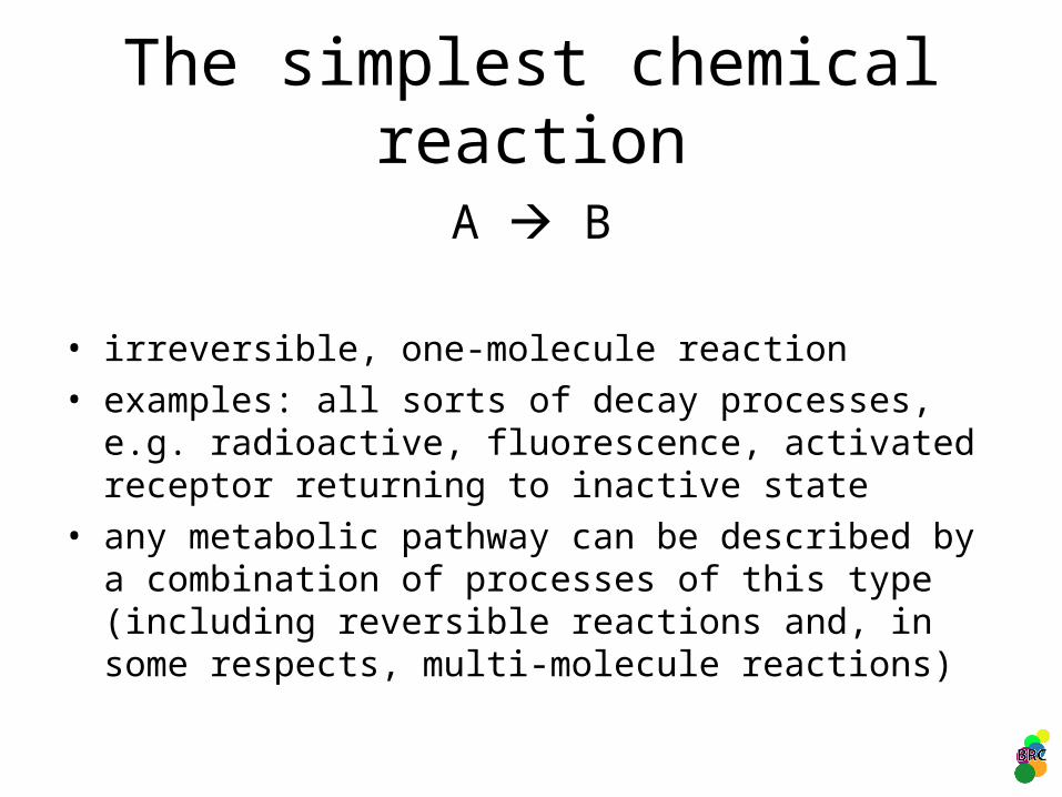
The simplest chemical reaction

A B

• irreversible, one-molecule reaction• examples: all sorts of decay processes, e.g. radioactive,

fluorescence, activated receptor returning to inactive state

• any metabolic pathway can be described by a combination of processes of this type (including reversible reactions and, in some respects, multi-molecule reactions)

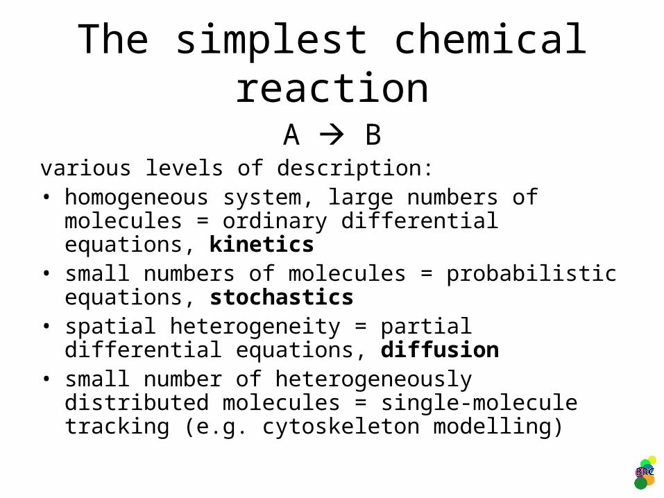
The simplest chemical reaction

A Bvarious levels of description:• homogeneous system, large numbers of molecules =

ordinary differential equations, kinetics• small numbers of molecules = probabilistic equations,

stochastics• spatial heterogeneity = partial differential equations,

diffusion• small number of heterogeneously distributed molecules

= single-molecule tracking (e.g. cytoskeleton modelling)

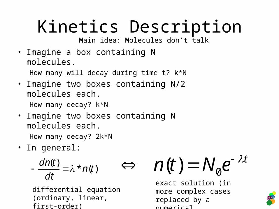
Kinetics Description• Imagine a box containing N molecules.

How many will decay during time t? k*N

• Imagine two boxes containing N/2 molecules each. How many decay? k*N

• Imagine two boxes containing N molecules each.How many decay? 2k*N

• In general:

)(*)(

tndt

tdn

Main idea: Molecules don’t talk

teNtn 0)(differential equation (ordinary, linear, first-order)

exact solution (in more complex cases replaced by a numerical approximation)

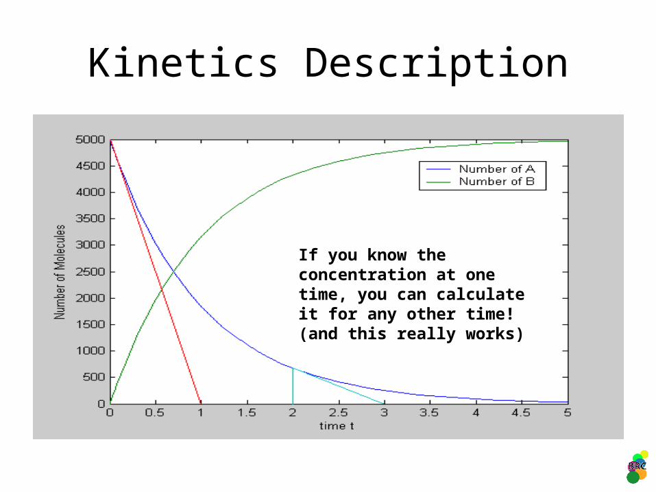
Kinetics Description

If you know the concentration at one time, you can calculate it for any other time! (and this really works)

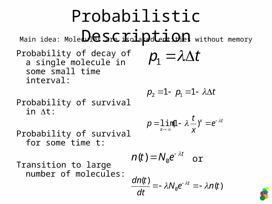
Probabilistic Description

Probability of decay of a single molecule in some small time interval:

Probability of survival in t:

Probability of survival for some time t:

Transition to large number of molecules:

tp 1

tpp 11 12

tx

xe

x

tp

)1(lim

teNtn 0)(

)()(

0 tneNdt

tdn t

or

Main idea: Molecules are isolated entities without memory

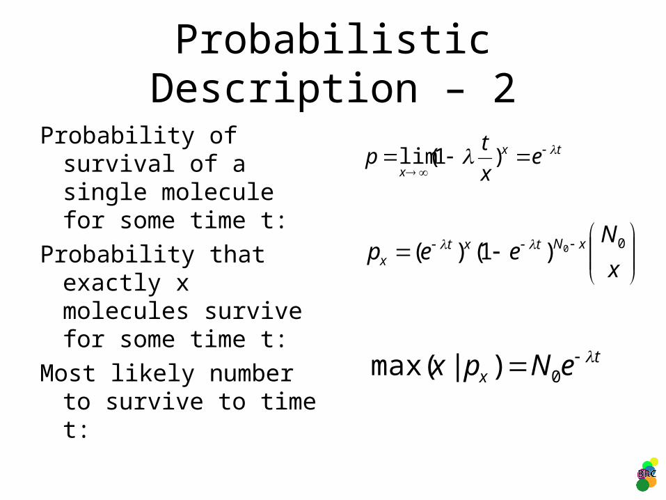
Probabilistic Description – 2

Probability of survival of a single molecule for some time t:

Probability that exactly x molecules survive for some time t:

Most likely number to survive to time t:

tx

xe

x

tp

)1(lim

x

Neep xNtxt

x00)1()(

tx eNpx 0)|max(

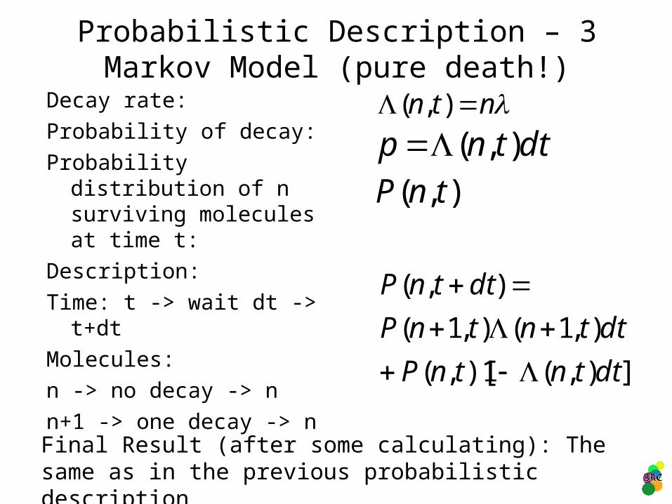
Probabilistic Description – 3Markov Model (pure death!)

Decay rate:

Probability of decay:

Probability distribution of n surviving molecules at time t:

Description:

Time: t -> wait dt -> t+dt

Molecules:

n -> no decay -> n

n+1 -> one decay -> n

ntn ),(

dttnp ),(),( tnP

]),(1)[,(

),1(),1(

),(

dttntnP

dttntnP

dttnP

Final Result (after some calculating): The same as in the previous probabilistic description

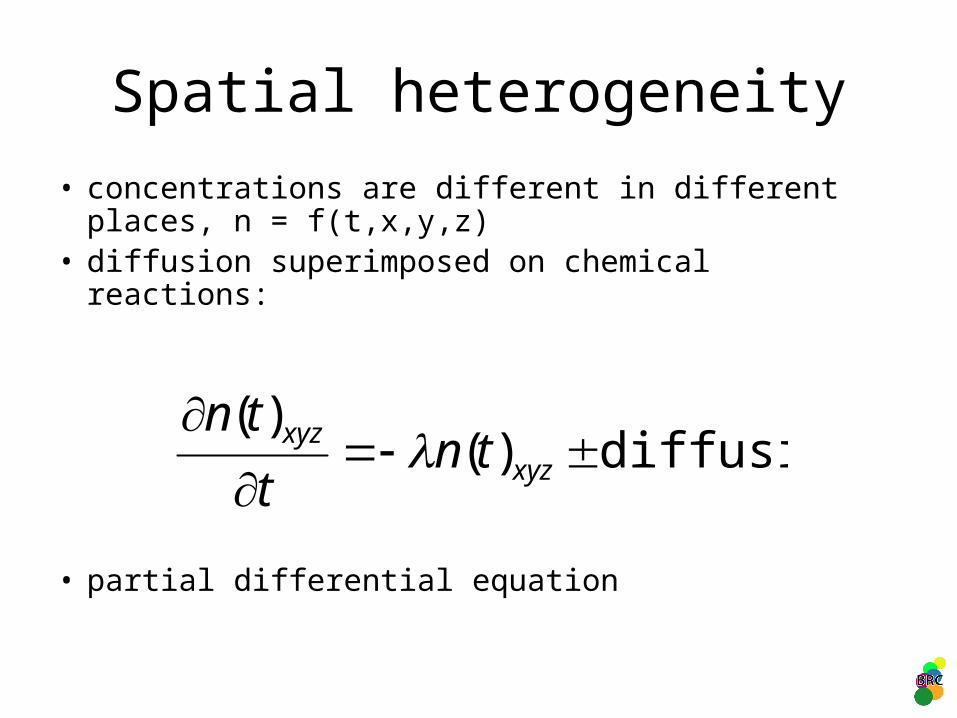
Spatial heterogeneity

• concentrations are different in different places, n = f(t,x,y,z)

• diffusion superimposed on chemical reactions:

• partial differential equation

diffusion)()(

xyz

xyz tnt

tn

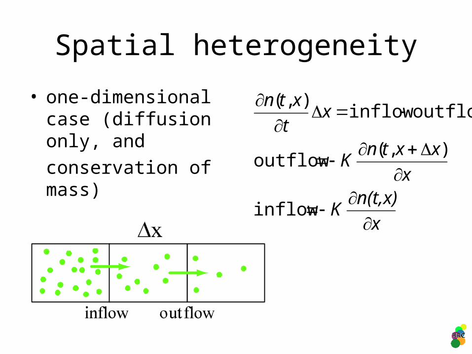
Spatial heterogeneity

• one-dimensional case (diffusion only, and

conservation of mass)

x

n(t,x)K

x

xxtnK

xt

xtn

inflow

),(outflow

outflowinflow),(

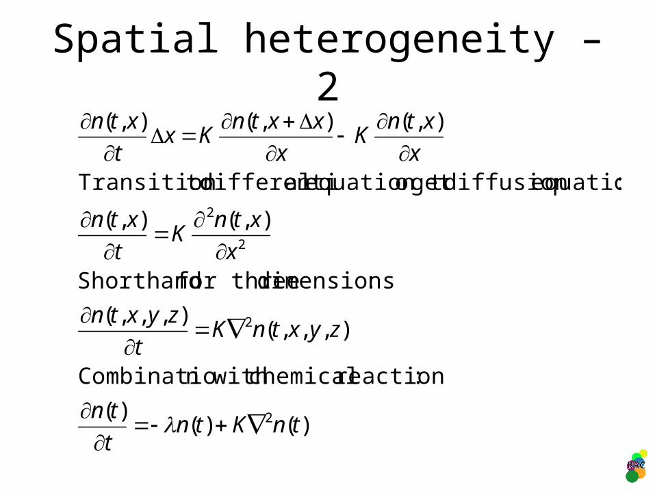
Spatial heterogeneity – 2

)()()(

:reaction chemicaln with Combinatio

),,,(),,,(

:dimensions for three Shorthand

),(),(

:equationdiffusion get oequation t aldifferenti toTransition

),(),(),(

2

2

2

2

tnKtnt

tn

zyxtnKt

zyxtn

x

xtnK

t

xtn

x

xtnK

x

xxtnKx

t

xtn

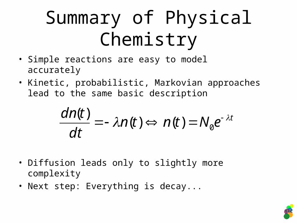
Summary of Physical Chemistry

• Simple reactions are easy to model accurately• Kinetic, probabilistic, Markovian approaches lead to

the same basic description

• Diffusion leads only to slightly more complexity• Next step: Everything is decay...

teNtntndt

tdn 0)()()(

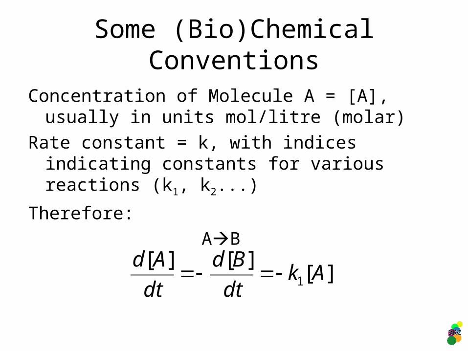
Some (Bio)Chemical Conventions

Concentration of Molecule A = [A], usually in units mol/litre (molar)

Rate constant = k, with indices indicating constants for various reactions (k1, k2...)

Therefore:

AB

][][][

1 Akdt

Bd

dt

Ad

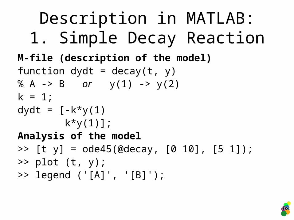
Description in MATLAB:1. Simple Decay Reaction

M-file (description of the model)function dydt = decay(t, y)% A -> B or y(1) -> y(2)k = 1;dydt = [-k*y(1) k*y(1)];Analysis of the model>> [t y] = ode45(@decay, [0 10], [5 1]);>> plot (t, y);>> legend ('[A]', '[B]');

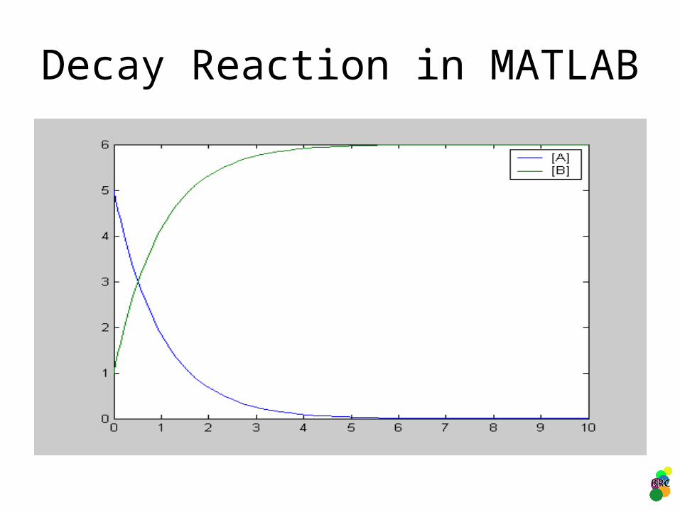
Decay Reaction in MATLAB

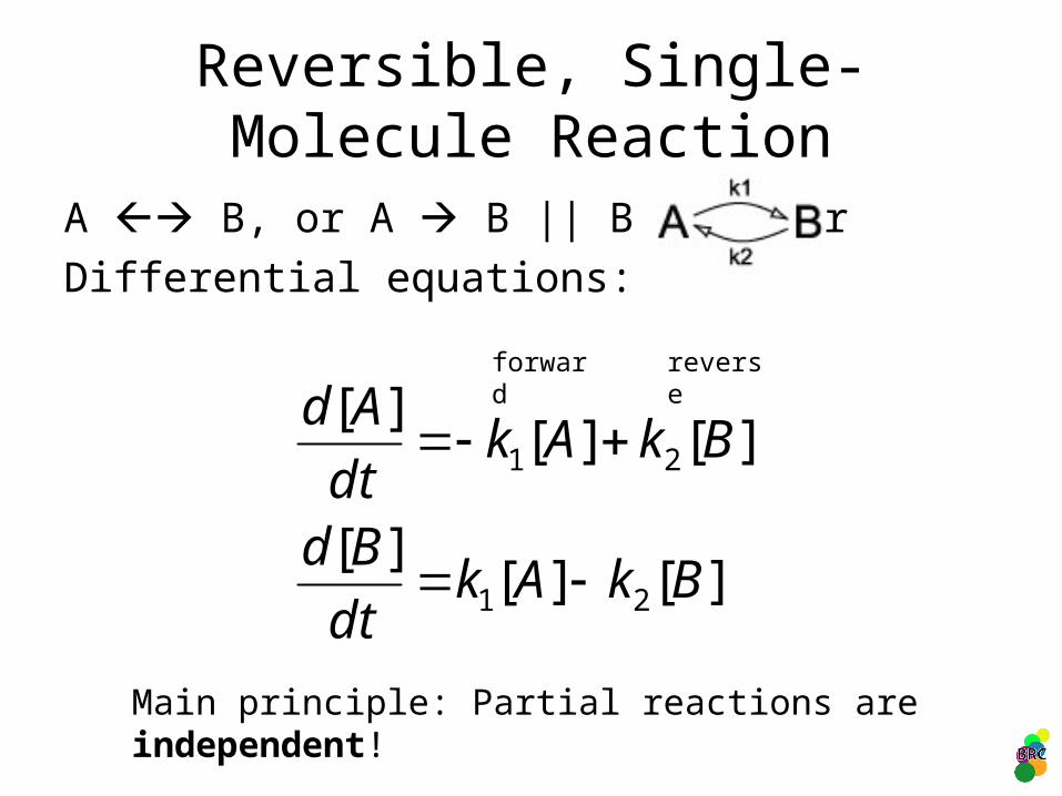
Reversible, Single-Molecule Reaction

A B, or A B || B A, or

Differential equations:

][][][

][][][

21

21

BkAkdt

Bd

BkAkdt

Ad

forward reverse

Main principle: Partial reactions are independent!

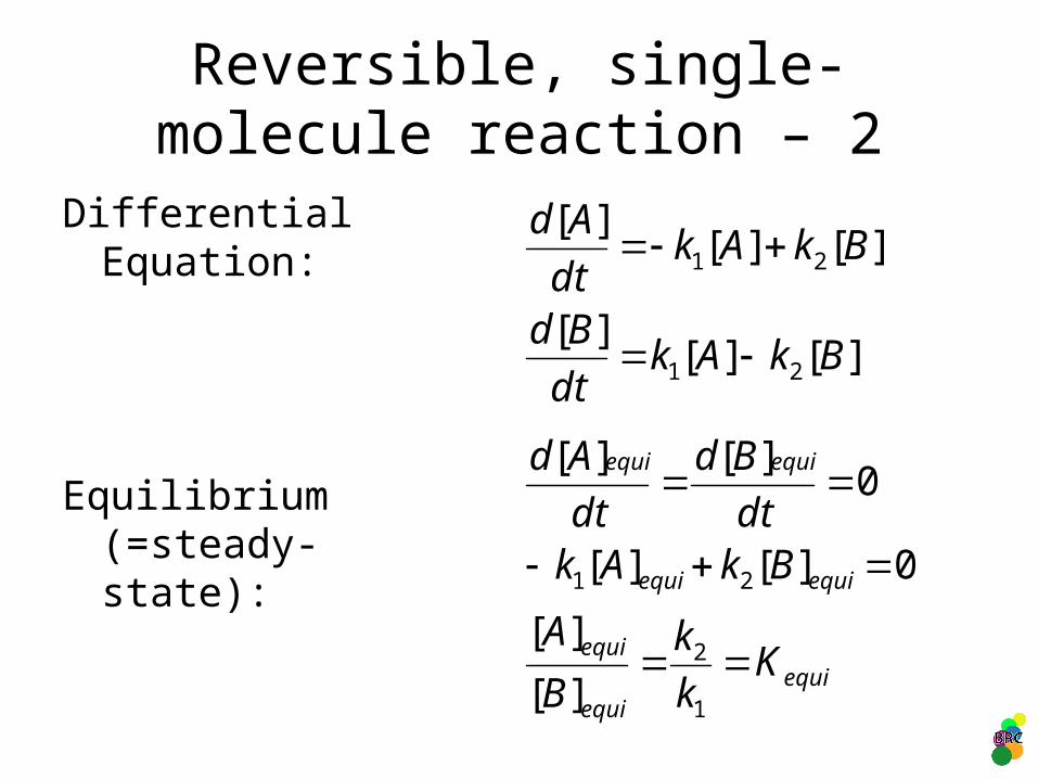
Reversible, single-molecule reaction – 2

Differential Equation:

Equilibrium (=steady-state):

equiequi

equi

equiequi

equiequi

Kk

k

B

A

BkAkdt

Bd

dt

Ad

1

2

21

][

][

0][][

0][][

][][][

][][][

21

21

BkAkdt

Bd

BkAkdt

Ad

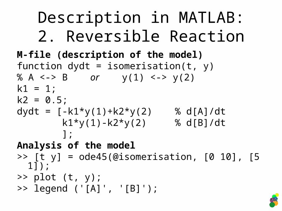
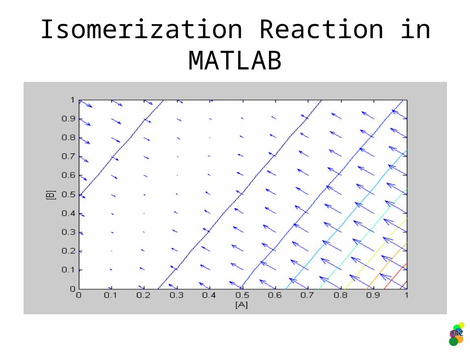
Description in MATLAB:2. Reversible Reaction

M-file (description of the model)function dydt = isomerisation(t, y)% A <-> B or y(1) <-> y(2)k1 = 1;k2 = 0.5;dydt = [-k1*y(1)+k2*y(2) % d[A]/dt k1*y(1)-k2*y(2) % d[B]/dt ];Analysis of the model>> [t y] = ode45(@isomerisation, [0 10], [5 1]);

>> plot (t, y);>> legend ('[A]', '[B]');

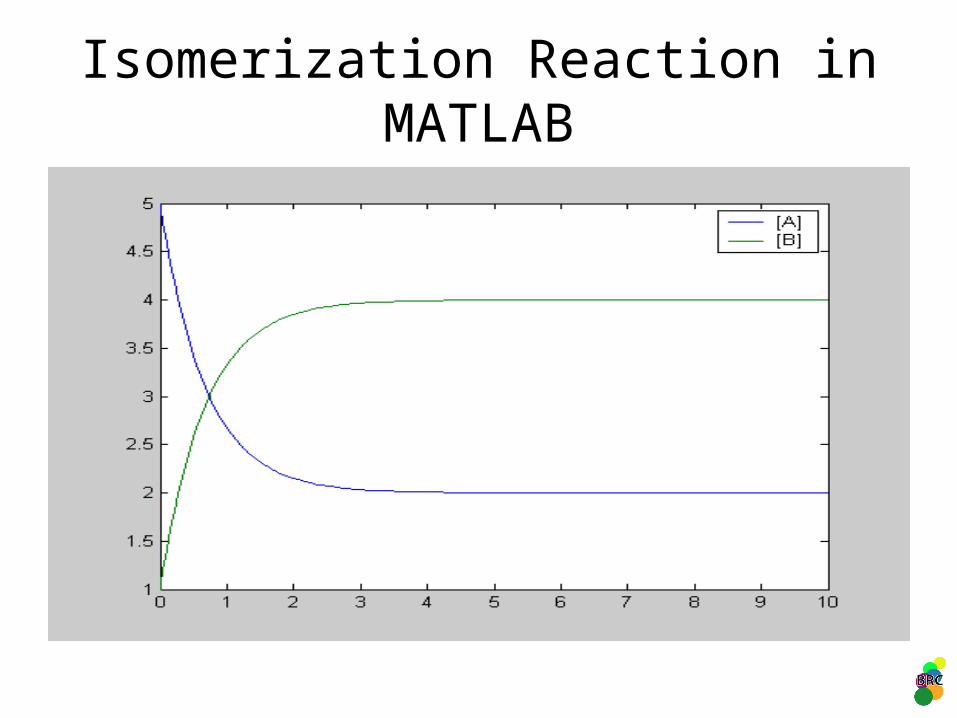
Isomerization Reaction in MATLAB

Isomerization Reaction in MATLAB

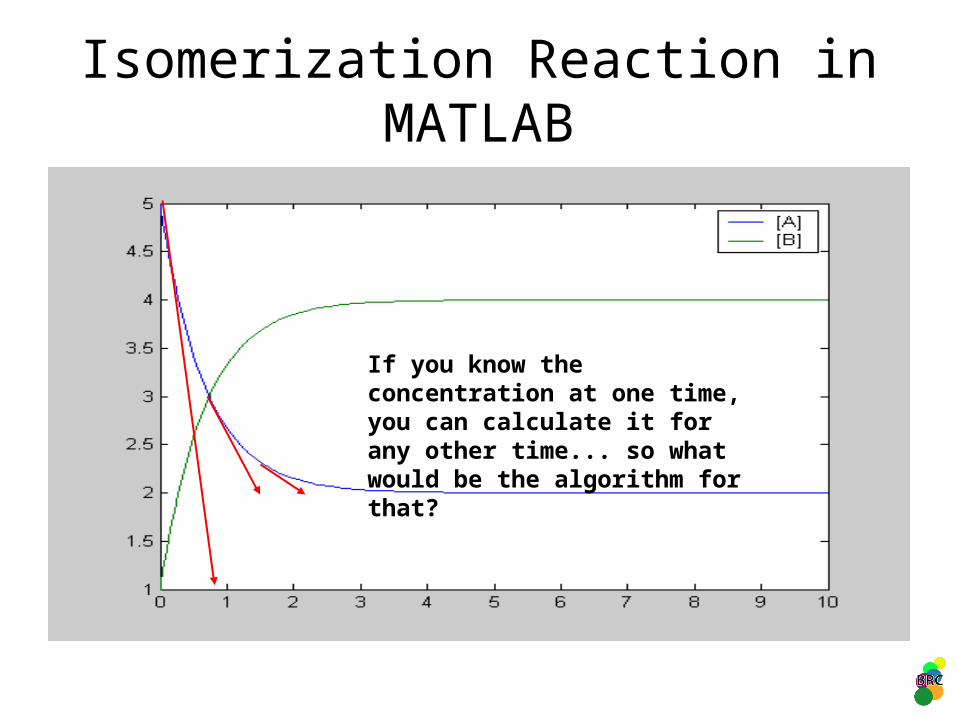
If you know the concentration at one time, you can calculate it for any other time... so what would be the algorithm for that?

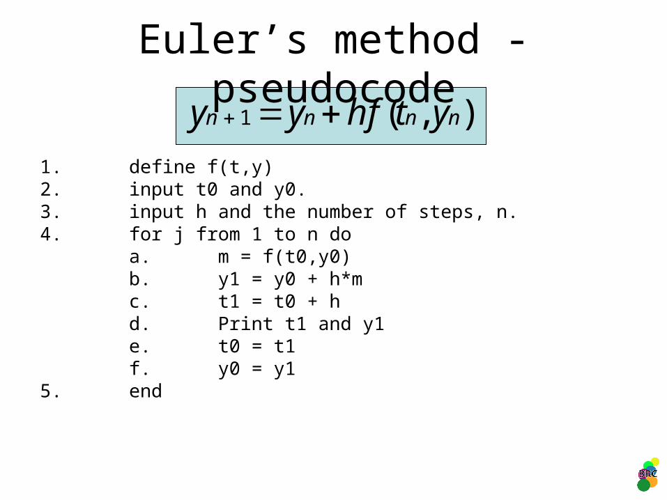
Euler’s method - pseudocode

1. define f(t,y)2. input t0 and y0.3. input h and the number of steps, n.4. for j from 1 to n do a. m = f(t0,y0) b. y1 = y0 + h*m c. t1 = t0 + h d. Print t1 and y1 e. t0 = t1 f. y0 = y15. end

),(1 nnnn ythfyy

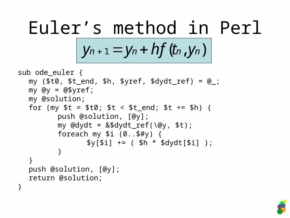
Euler’s method in Perl

sub ode_euler {my ($t0, $t_end, $h, $yref, $dydt_ref) = @_;my @y = @$yref;my @solution;for (my $t = $t0; $t < $t_end; $t += $h) {

push @solution, [@y];my @dydt = &$dydt_ref(\@y, $t);foreach my $i (0..$#y) {

$y[$i] += ( $h * $dydt[$i] );}

}push @solution, [@y];return @solution;

}

),(1 nnnn ythfyy

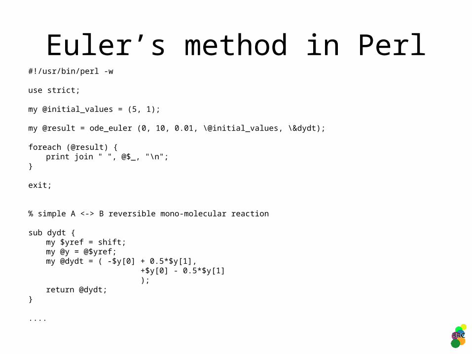
Euler’s method in Perl#!/usr/bin/perl -w

use strict;

my @initial_values = (5, 1);

my @result = ode_euler (0, 10, 0.01, \@initial_values, \&dydt);

foreach (@result) {print join " ", @$_, "\n";

}

exit;

% simple A <-> B reversible mono-molecular reaction

sub dydt {my $yref = shift;my @y = @$yref;my @dydt = ( -$y[0] + 0.5*$y[1],

+$y[0] - 0.5*$y[1]);

return @dydt;}

....

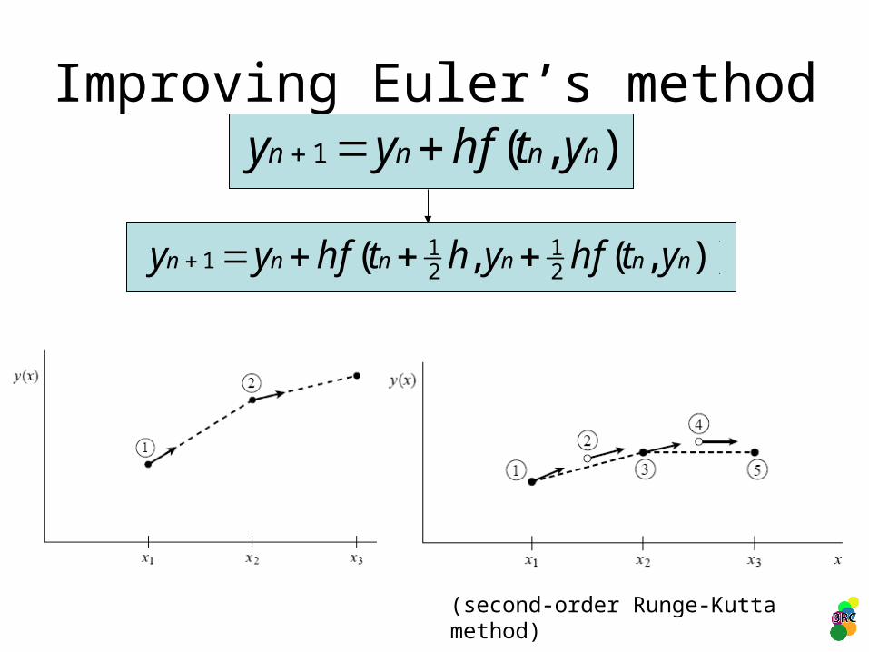
Improving Euler’s method

)),(,( 21

21

1 nnnnnn ythfyhthfyy

),(1 nnnn ythfyy

(second-order Runge-Kutta method)

Isomerization Reaction in MATLAB

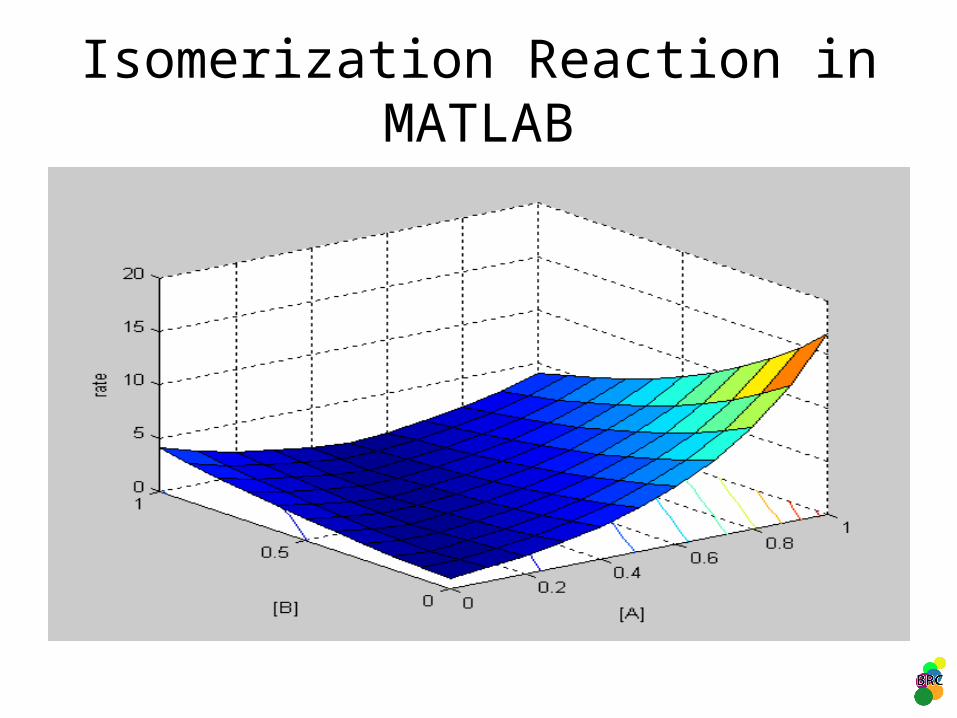
Isomerization Reaction in MATLAB

Irreversible, two-molecule reaction

A+BC

Differential equations:

]][[][

][][][

BAkdt

Addt

Cd

dt

Bd

dt

Ad

Underlying idea: Reaction probability = Combined probability that both [A] and [B] are in a “reactive mood”:

]][[][][)()()( *2

*1 BAkBkAkBpApABp

The last piece of the puzzle

Non-linear!

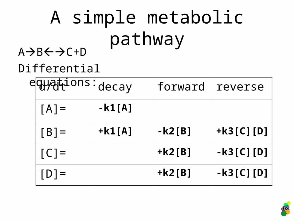
A simple metabolic pathwayABC+D

Differential equations:

d/dt decay forward reverse

[A]= -k1[A]

[B]= +k1[A] -k2[B] +k3[C][D]

[C]= +k2[B] -k3[C][D]

[D]= +k2[B] -k3[C][D]

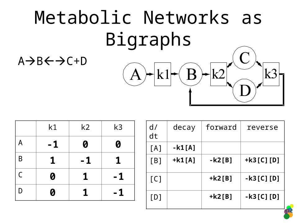
Metabolic Networks as Bigraphs

ABC+D

d/dt decay forward reverse

[A] -k1[A]

[B] +k1[A] -k2[B] +k3[C][D]

[C] +k2[B] -k3[C][D]

[D] +k2[B] -k3[C][D]

k1 k2 k3

A -1 0 0B 1 -1 1C 0 1 -1D 0 1 -1

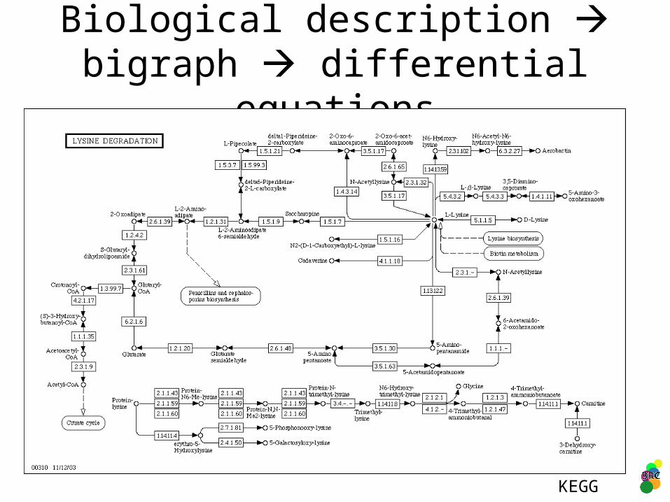
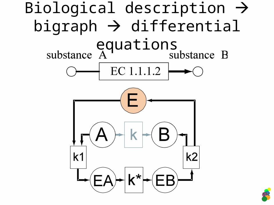
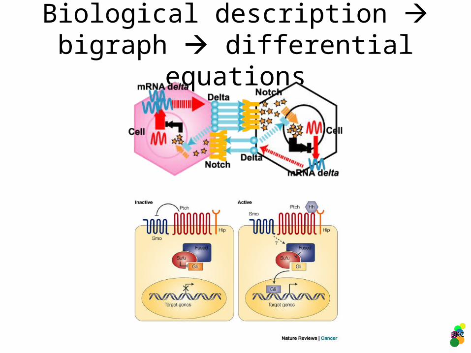
Biological description bigraph differential equations

KEGG

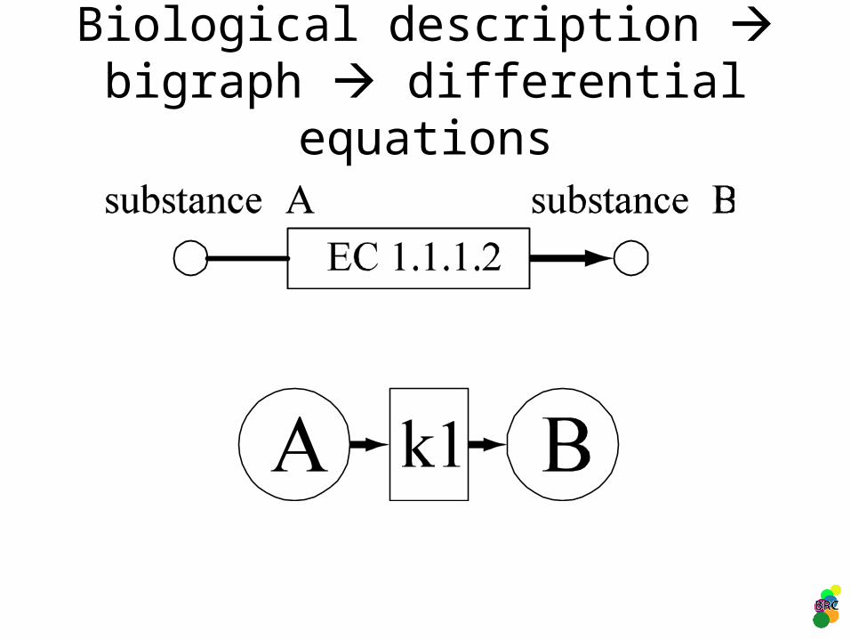
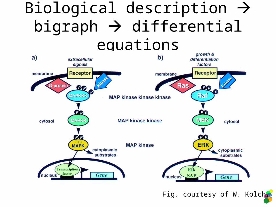
Biological description bigraph differential equations

Biological description bigraph differential equations

Biological description bigraph differential equations

Biological description bigraph differential equations

Fig. courtesy of W. Kolch

Biological description bigraph differential equations

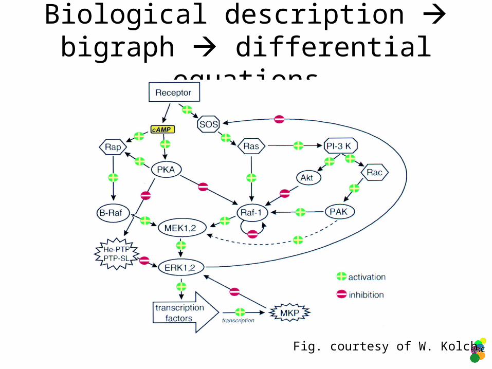
Fig. courtesy of W. Kolch

Biological description bigraph differential equations

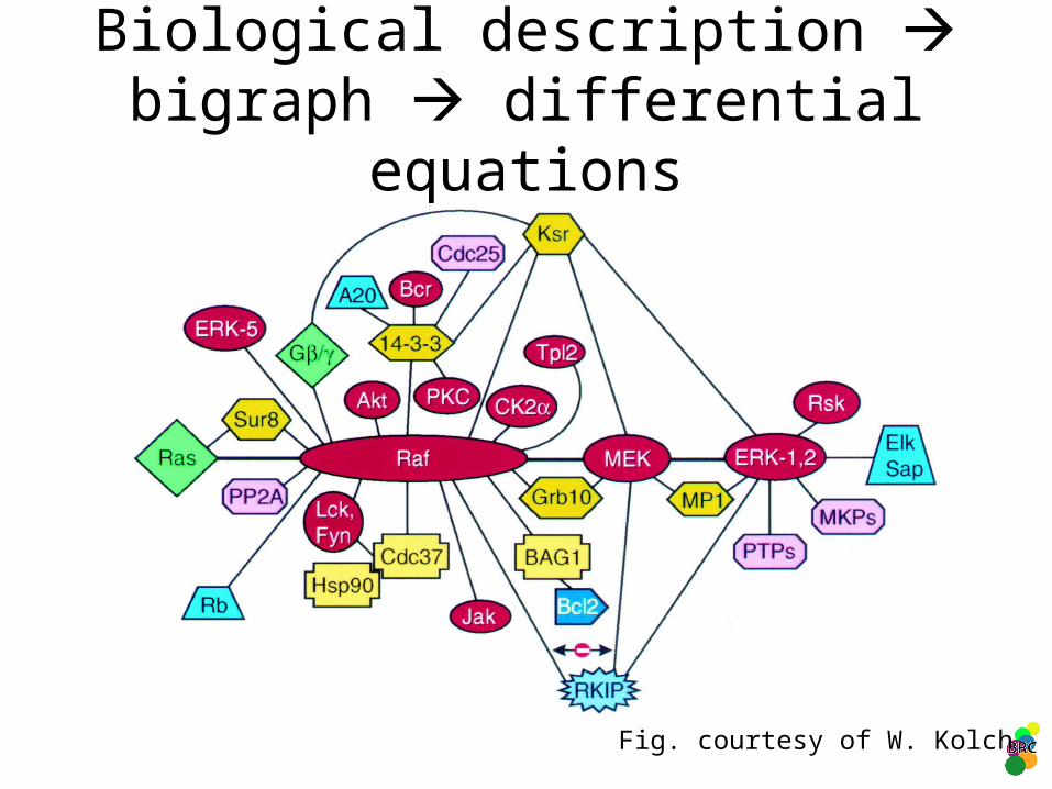
Fig. courtesy of W. Kolch

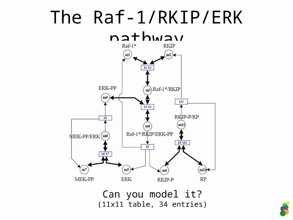
The Raf-1/RKIP/ERK pathway

Can you model it?(11x11 table, 34 entries)

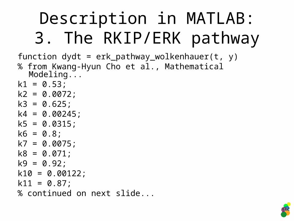
Description in MATLAB:3. The RKIP/ERK pathway

function dydt = erk_pathway_wolkenhauer(t, y)% from Kwang-Hyun Cho et al., Mathematical

Modeling... k1 = 0.53;k2 = 0.0072;k3 = 0.625;k4 = 0.00245;k5 = 0.0315;k6 = 0.8;k7 = 0.0075;k8 = 0.071;k9 = 0.92;k10 = 0.00122;k11 = 0.87;% continued on next slide...

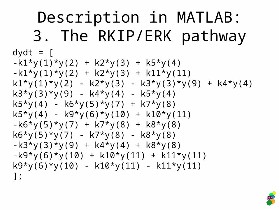
Description in MATLAB:3. The RKIP/ERK pathway

dydt = [-k1*y(1)*y(2) + k2*y(3) + k5*y(4)-k1*y(1)*y(2) + k2*y(3) + k11*y(11)k1*y(1)*y(2) - k2*y(3) - k3*y(3)*y(9) + k4*y(4)k3*y(3)*y(9) - k4*y(4) - k5*y(4)k5*y(4) - k6*y(5)*y(7) + k7*y(8)k5*y(4) - k9*y(6)*y(10) + k10*y(11)-k6*y(5)*y(7) + k7*y(8) + k8*y(8)k6*y(5)*y(7) - k7*y(8) - k8*y(8)-k3*y(3)*y(9) + k4*y(4) + k8*y(8)-k9*y(6)*y(10) + k10*y(11) + k11*y(11)k9*y(6)*y(10) - k10*y(11) - k11*y(11)];

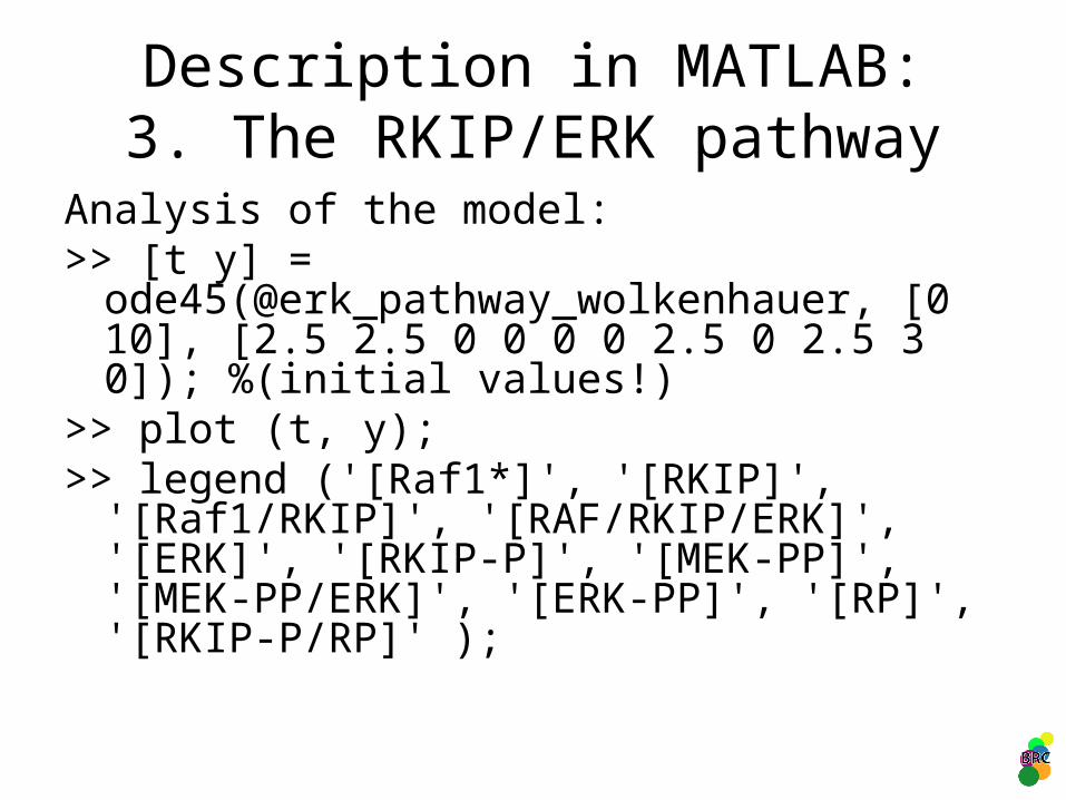
Description in MATLAB:3. The RKIP/ERK pathway

Analysis of the model:>> [t y] = ode45(@erk_pathway_wolkenhauer, [0 10], [2.5 2.5 0 0 0 0 2.5 0 2.5 3 0]); %(initial values!)

>> plot (t, y);>> legend ('[Raf1*]', '[RKIP]', '[Raf1/RKIP]', '[RAF/RKIP/ERK]', '[ERK]', '[RKIP-P]', '[MEK-PP]', '[MEK-PP/ERK]', '[ERK-PP]', '[RP]', '[RKIP-P/RP]' );

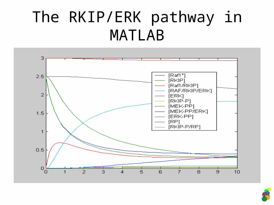
The RKIP/ERK pathway in MATLAB

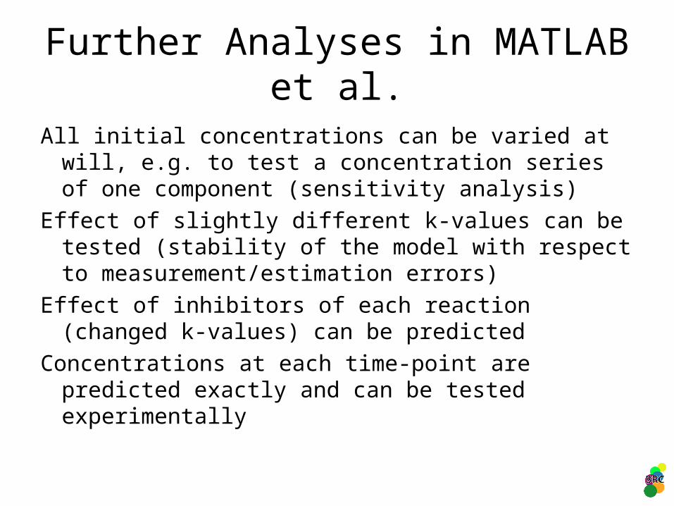
Further Analyses in MATLAB et al.

All initial concentrations can be varied at will, e.g. to test a concentration series of one component (sensitivity analysis)

Effect of slightly different k-values can be tested (stability of the model with respect to measurement/estimation errors)

Effect of inhibitors of each reaction (changed k-values) can be predicted

Concentrations at each time-point are predicted exactly and can be tested experimentally

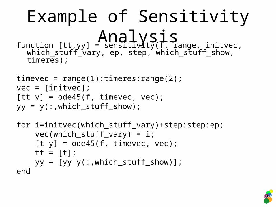
Example of Sensitivity Analysisfunction [tt,yy] = sensitivity(f, range, initvec,

which_stuff_vary, ep, step, which_stuff_show, timeres);

timevec = range(1):timeres:range(2);vec = [initvec];[tt y] = ode45(f, timevec, vec);yy = y(:,which_stuff_show);

for i=initvec(which_stuff_vary)+step:step:ep; vec(which_stuff_vary) = i; [t y] = ode45(f, timevec, vec); tt = [t]; yy = [yy y(:,which_stuff_show)];end

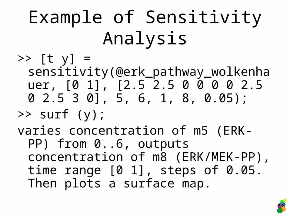
Example of Sensitivity Analysis

>> [t y] = sensitivity(@erk_pathway_wolkenhauer, [0 1], [2.5 2.5 0 0 0 0 2.5 0 2.5 3 0], 5, 6, 1, 8, 0.05);

>> surf (y);varies concentration of m5 (ERK-PP) from

0..6, outputs concentration of m8 (ERK/MEK-PP), time range [0 1], steps of 0.05. Then plots a surface map.

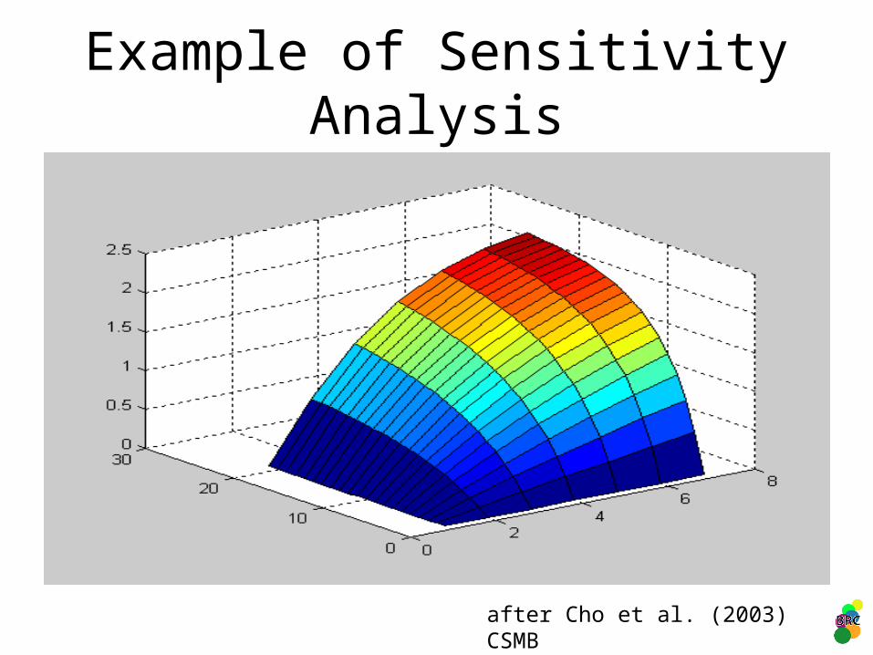
Example of Sensitivity Analysis

after Cho et al. (2003) CSMB

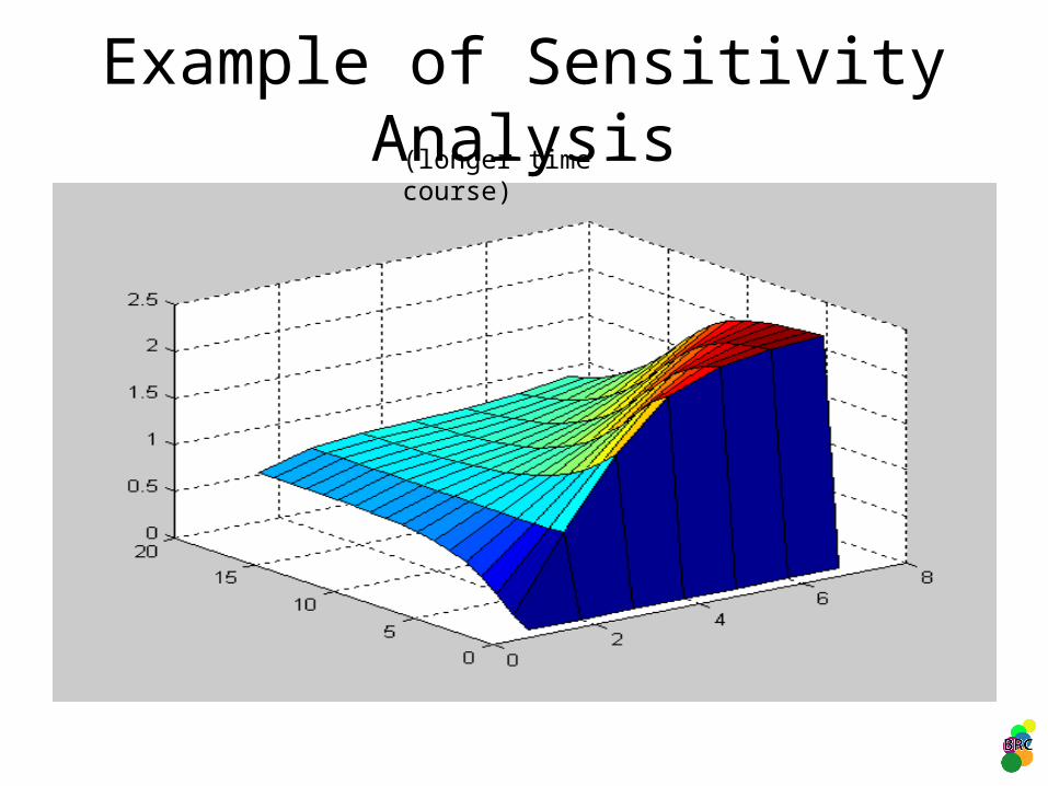
Example of Sensitivity Analysis(longer time course)

Conclusions and Outlook

• differential equations allow exact predictions of systems behaviour in a unified formalism

• modelling = in silico experimentation• difficulties:

– translation from biology• modular model building interfaces, e.g. Gepasi/COPASI, Genomic

Object Net, E-cell, Ingeneue– managing complexity explosion

• pathway visualization and construction software• standardized description language, e.g. Systems Biology Markup

Language (SBML)– lack of biological data

• perturbation-based parameter estimation, e.g. metabolic control analysis (MCA)

• constraints-based modelling, e.g. flux balance analysis (FBA)• semi-quantitative differential equations for inexact knowledge