lstm neural network with emotional analysis for prediction ... · stock opening price being the...

Abstract—Time series forecasting is an important and widely

known topic in the research of statistics, with the forecasting of

stock opening price being the most crucial element in the entire

forecasting process. However, to improve the accuracy of

forecasting the stock opening price is a challenging task,

therefore in this paper, we propose a robust time series learning

model for prediction of stock opening price. The proposed model

consists of two parts, namely the emotional analysis model and

the long short-term memory (LSTM) time series learning model.

Firstly, we use an emotion classifier based on naïve Bayesian to

analyze the data from forums. Secondly, we combine the

emotional data obtained from the previous experiments together

with the actual Behavior Data as the training data for the long

short-term memory time series learning model. Finally, a

satisfactory result can be obtained by training the neural

network. Experimental results show that by treating the stock

exchange data, Shanghai Composite index and emotional data as

the input variables can greatly improve the prediction accuracy.

As expected, an outstanding prediction performance has been

obtained from proposed model as it outperforms traditional

neural network. The proposed model is expected to be a

promising method in the realm of stock opening price prediction

where the data are non-linear, long-term dependent and

influenced by noise and many other factors.

Index Terms—stock forecasting, LSTM, emotional analysis,

time series

I. INTRODUCTION

IME series forecasting is an interdisciplinary research

program which has some useful applications in a

numerous of other research fields. In the financial area, time

series forecasting can help people make a wise plan and

decision so as to reduce the risk of investment. In a time series,

time is usually an important variable used for making

decisions and predictions. When we use time series to predict

the trend of the future, we need to utilize detailed historical

data over a period of time to understand it. Researchers

usually use historical data to predict various future events,

such as the forecast of stock prices and changes of product

sales.

Many traditional methods based on statistics are proposed

for time series learning. These methods include linear

regression [1], Moving Average (MA) and Auto-regression

(AR). Box and Jenkins [2] proposed Auto-regression Moving

Qun Zhuge is with the School of Computer Engineering and Science,

Shanghai University, 200444 China (e-mail: [email protected]).

Lingyu Xu is professor with the School of Computer Engineering and

Science, Shanghai University, 200444 China (e-mail: [email protected]).

Gaowei Zhang is with the school of Computer Engineering and Science,

Shanghai University, 200444 China (e-mail:[email protected]).

Average (ARMA) model that can deal with the sequence, part

of which is Auto-regression while another part is Moving

Average. Auto-regression Integrated Moving Average

(ARIMA) model [2] is capable of dealing with non-stationary

time series. Engle [3] established Auto-regressive

Conditional Heteroskedasticity (ARCH) model, which can

simulate the variation of time series variable. Thereafter,

Bolleralev [4] proposed Generalized Autoregressive

Conditional Heteroskedasticity (GARCH) model, which is

particularly suitable for the analysis and prediction of

volatility. These methods are widely used in the field of time

series predictions and can achieve a good predictive effect

when the time series is Gauss distribution. Some other

traditional methods are also used for time series forecasting.

Elaal et al. introduced multivariate-factors fuzzy time series

forecasting model based on fuzzy clustering to handle

real-world multivariate forecasting problems [5]. Khalil

Khiabani and Saeed Reza Aghabozorgi presented hybrid

forecast model based on the particle swarm optimization and

k-means clustering to solve time series forecasting problems

[6]. However, there are still a few drawbacks regarding the

previously mentioned models where they are not able to take

the unstable and non-stationary factors of the stock

forecasting into account [7].

Artificial neural network (ANN) [8] is one of the most

accurate methods to predict stock trends. So far, ANN has

been widely used in stock forecasting [9]. Shen, Guo, Wu, and

Wu [10] predict stock indices of Shanghai Stock Exchange

with the model of radial basis function neural network.

Huarng and Yu [11] used back-propagation neural network to

predict stock price. Some researchers regard stock price as

time series [12], [13] and use short-term memory model

Recurrent Neural Network (RNN) to forecast time series [14],

[15].

Based on the findings above, these models exist three main

disadvantages. (1) The traditional time series models use

historical stock data as the input variables. However, the price

of stock is affected by a large number of factors, such as

market conditions and environmental influences. The direct

use of complex historical data in the traditional time series

models has a tendency to reduce the forecasting ability and

therefore the final results. Therefore, many researchers tend to

reduce the complexity of the original data, for instance,

principal component analysis (PCA) is proposed so that the

original data break down into simpler elements or higher

correlated variables to improve the ability of the predicting

models. (2) These models only take the historical trade data as

input variables, but not considering the impacts of the

environment of the stock on the forecasting, such as the

LSTM Neural Network with Emotional Analysis

for Prediction of Stock Price

Qun Zhuge, Lingyu Xu and Gaowei Zhang

T

Engineering Letters, 25:2, EL_25_2_09

(Advance online publication: 24 May 2017)

______________________________________________________________________________________

emotional tendency of investors. (3) Some researchers do not

regard stock price variables as a time series and consider them

as discrete variations. Other researchers even consider stock

price variations as a time series, but they believe the memory

of time series is either short or fixed. Yet, as seen above, the

long-term dependence problems are not well handled.

To overcome the drawbacks above, we propose a robust

time series learning model for predictions of stock opening

price. The proposed model consists of two models: the

emotional analysis model and the long short-term memory

(LSTM) time series learning model. Research shows that

network information can be used to predict product sales,

brand awareness and presidential election, etc. Mishne and

Rijke [16] used the number of the blog comments to calculate

box office whereas Schumaker and Chen [17] studied the

correlation between financial news and stock prices. Long

Short-Term Memory (LSTM) is a variant of RNN and proves

to be demonstrating good performances in time series

learning as LSTM can maintain contextual information as

well as temporal behaviors of events. In this paper, we

integrate data from network public opinions and actual

behavior data as a high dimension input time series, and

propose a new time series model based on long short-term

memory. This new model trains the input data to deduce the

price of the stock.

We use corresponding network of public opinions data to

establish emotion classifier based on naïve Bayes. Then, we

post the information of shares into the emotion classifier to

get the emotional data on stock. After that, we combine the

emotional data and the actual behavior data to establish a high

dimension time series. Finally, we train the model so that it is

capable of predicting the results from the original data.

Experimental results suggest that the proposed model can

achieve significant effectiveness in stock forecasting.

The remaining parts of this paper is organized as the

following: Section 2 will describe the related studies. Section

3 will briefly introduce the basic definitions of the new model

where Section 4 introduces the time series learning based on

LSTM. Section 5 shows and discusses the experimental

results. Finally, conclusions are made in Section 6.

II. RELATED WORK

Predicting stock price is an exciting and challenging

research [18]. Many time series forecasting models have been

proposed to be used for stock forecasting. First of all, we will

review the application of ANN in stock forecasting because

many studies show that ANN outperforms statistical

regression models [19] and discriminant analysis [20]. Wang,

Zou, Su, Li, & Chaudhry [21] proposed a time series

prediction model based on ARIMA and ANN. In another

study, Rout, Majhi, Majhi, and Panda [22] developed a model

by ARIMA and differential evolution based on trainings of

ANN. In a recent study, Yi, Jin, John, and Shouyang [23] used

ARIMA and ANN to predict the financial volatility. These

models are combined with statistical and ANN. At the same

time there are a number of studies conducted in a bid to

optimize the parameters of ANN. Kim and Ahn [24] tried to

find a global optimal solution of ANN. Chen, Fan, Chen, and

Wei [25] designed experiments on ANN’s parameters

optimization in stock forecasting.

Furthermore, many Neural Networks for time series have

been brought into the use of stock forecasting. Chen, Leung,

and Daouk [26] used probabilistic neural network (PNN) to

predict the direction of index return. Huarng and Yu [27] used

BP neural network to forecast stock price. In another research,

Hsu [28] used BP neural network and feature selection as well

as genetic programming to solve the problems of stock price

forecasting. In the latest studies, Time series model RNN with

short-term memory is widely used. Hsieh, Hsiao, and Yeh [29]

merged wavelet transforms and RNN based on artificial bee

colony algorithm to predict stock markets.

III. DEFINITION OF MODEL

Stock market can be seen as a group decision making

system, subject to external (Network Public Opinion) as well

as internal (Actual Behavior) constraints. Therefore, the

whole system can be divided into two space. One space is

Network Public Opinion Data Space (OS) and the other space

is Actual Behavior Data Space (BS).

A. Actual Behavior Data Space

The data we choose is composed of various attributes of

each stock and Shanghai Stock Composite Index (SCI). We

define the BS:

S S S SBS={Time,Member,Price ,High ,Low ,Close }

S S S SH SH{Chg ,%Chg ,%Turnover ,Close ,High }

SH SH SH SH{Low ,Price ,Chg ,%Chg } (1)

Where Time denotes the trading time of the listing

Corporation’s shares, Member denotes the ticker of the listing

Corporation’s shares, SPrice denotes the opening price of

stock at Time , SHigh denotes maximum price of stock at

Time, SLow denotes minimum price of the stock at Time,

CloseS denotes closing price of the stock at Time, ChgS

denotes change amount of stock at Time, %ChgS denotes

change rate of stock at Time, %TurnoverS denotes turnover

rate of stock at Time, SHClose denotes closing price of

Shanghai Composite Index at Time, SHHigh denotes

maximum price of Shanghai Composite Index at Time,

SHLow denotes minimum price of Shanghai Composite Index

at Time, SHPrice denotes opening price of Shanghai

Composite Index at Time, SHChg denotes change amount of

Shanghai Composite Index at Time, SH%Chg denotes change

rate of Shanghai Composite Index at Time.

B. Network Public Opinion Data Space

The outstanding feature of the Internet is to connect each

isolated computer into the network, so as to realize the high

speed transmission and sharing of global information. There

is a lot of network evaluation information in the network

public opinion space, which often contains a lot of emotional

tendency, so we generally call it information emotional

tendency. Information emotional tendency has the following

characteristics: 1) Memory. Investor sentiment information

both has the special features of the financial information and

has the semantic features of the text information. Once this



______________________________________________________________________________________

information appears in the network public opinion, it will

leave traces in the network space, so it can be stored and be

remembered. 2) Spontaneity. As the subjective evaluation and

self-judgment of the information of the stock market and

listing Corporation, the investor sentiment in the network

space of public opinion is the spontaneous behavior of the

investors. This spontaneous generation, spontaneous

communication and spontaneous acceptance allow us to get a

more pure investor sentiment that is not affected by other

information. 3) Interactivity. The network evaluation

information in the network public opinion space both has the

objective description of all kinds of information and has the

subjective judgment of investors. The interactive process in

the network public opinion space, including investor's

attention, click and reply, makes the mood contained in the

network evaluation information have more tendencies. Due to

the widespread attention of investors, this interaction has an

unprecedented influence on the investor groups. 4)

Representativeness. The opinion of network evaluation

information in network public opinion space is generally

considered as the opinion that is held or recognized by the

information publisher, so this information represents clear

emotional tendencies of different investors. Although the

network public opinion revealed that the emotional focus of

investors is emanative, the object we focus on is concentrated,

which contains all kinds of information about the recent

performance and future development of quoted company. So

we can extract the performance characteristics of the investor

sentiment in the network public opinion space.

The comments information and reply message, which

crawled from the public message forum about the Shanghai

Composite Index of the Eastern wealth network, constitutes

the network of public opinion space. We defined information

of post as Posts, which is a subspace of OS.

Unlike in English, Most of the information from OS is in

the form of Chinese, so there is a space between each word.

For Chinese, we need to divide a sentence into several

meaningful words for further processing. In this paper, we

choose the Chinese lexical analysis system ICTCLAS

(Institute of Computing Technology, Chinese Lexical

Analysis System) to segment each information p in Posts of

OS. Each information p is represented as a collection of

words 1 2p={w ,w ,...,w }n , all of the information can be used to

form a sparse matrix P, whose rows and columns are labeled

with text and glossary, respectively.

Through manually labeled emotional information and

sentiment dictionary, we mark the emotional tendency of

information in the Posts of OS. We can filter out some

irrelevant nouns when dealing with the text information of

OS.

After processing, we can obtain a vector matrix P which is

used for training and the evaluation of the emotion classifier.

In this paper naïve Bayes method is used to set up an emotion

classifier. For the emotion tendency E={positive,negative}

obtained after processing the information 1 2p={w ,w ,...,w }n ,

considering the weight of the characteristics word, the

classification algorithm is as follows:

1

arg max{ ( ) ( | )}j

n

NB j i je E i

E P e P w e

(2)

Where ( )jP e denotes the prior probability of category je ;

( | )i jP w e denotes the posterior probability of the feature

word iw in the category je . For the prior probability ( )jP e , we

use the training corpus which has been correctly labeled to

estimate, and it is defined as:

( )( )

( )j

j

j

je E

n eP e

n e

(3)

Where ( )jn e denotes the number of information that

belongs to the category je .

Posterior probability ( | )i jP w e denotes the probability that

the characteristic word iw appears in the category je . The

ratio of iw 's total weight in the text labeled with je to all the

words' total weight in je is taken as an estimation of ( | )i jP w e .

We use TF-IDF value as the weight. In order to

avoid ( | )i jP w e value to be 0, this paper uses the Laplace

smoothing, so we can calculate the posterior probability as the

formula:

1

( , ) 1( | ) ,

( , )

i j

i j n

i j

i

weight w eP w e

weight w e

(4)

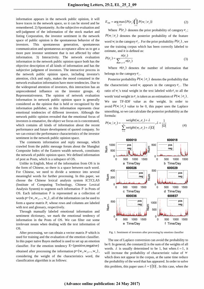
Fig. 1. Sentiment of investors after processing by emotion classifier

The use of Laplace conversion can avoid the probability to

be 0. In general, the constant is the sum of the weights of all

words. is usually determined to be 1, but when 1 , it

will increase the probability of characteristic value of w

which does not appear in the corpus, at the same time reduce

the probability of the word that has appeared. In order to solve

this problem, this paper uses 1 . In this case, when the



______________________________________________________________________________________

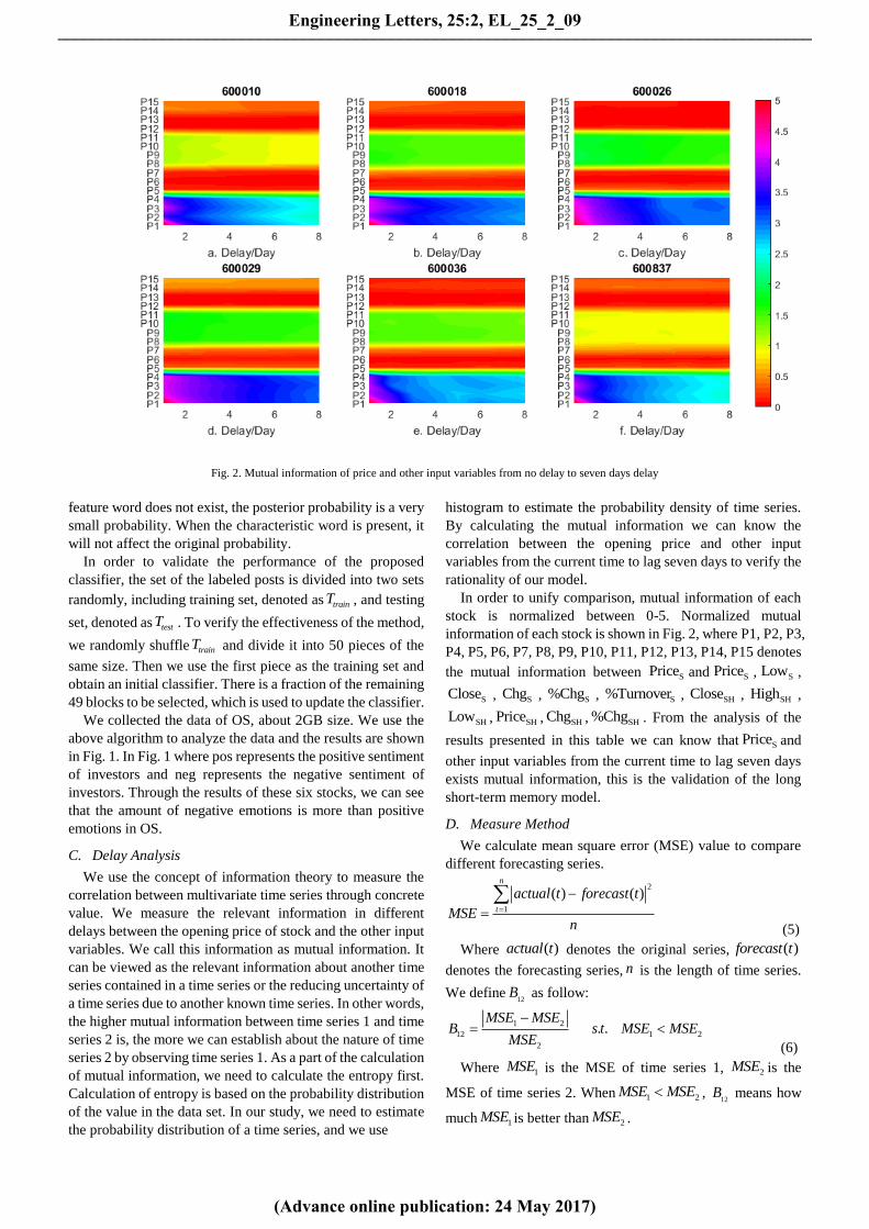
Fig. 2. Mutual information of price and other input variables from no delay to seven days delay

feature word does not exist, the posterior probability is a very

small probability. When the characteristic word is present, it

will not affect the original probability.

In order to validate the performance of the proposed

classifier, the set of the labeled posts is divided into two sets

randomly, including training set, denoted as trainT , and testing

set, denoted as testT . To verify the effectiveness of the method,

we randomly shuffle trainT and divide it into 50 pieces of the

same size. Then we use the first piece as the training set and

obtain an initial classifier. There is a fraction of the remaining

49 blocks to be selected, which is used to update the classifier.

We collected the data of OS, about 2GB size. We use the

above algorithm to analyze the data and the results are shown

in Fig. 1. In Fig. 1 where pos represents the positive sentiment

of investors and neg represents the negative sentiment of

investors. Through the results of these six stocks, we can see

that the amount of negative emotions is more than positive

emotions in OS.

C. Delay Analysis

We use the concept of information theory to measure the

correlation between multivariate time series through concrete

value. We measure the relevant information in different

delays between the opening price of stock and the other input

variables. We call this information as mutual information. It

can be viewed as the relevant information about another time

series contained in a time series or the reducing uncertainty of

a time series due to another known time series. In other words,

the higher mutual information between time series 1 and time

series 2 is, the more we can establish about the nature of time

series 2 by observing time series 1. As a part of the calculation

of mutual information, we need to calculate the entropy first.

Calculation of entropy is based on the probability distribution

of the value in the data set. In our study, we need to estimate

the probability distribution of a time series, and we use

histogram to estimate the probability density of time series.

By calculating the mutual information we can know the

correlation between the opening price and other input

variables from the current time to lag seven days to verify the

rationality of our model.

In order to unify comparison, mutual information of each

stock is normalized between 0-5. Normalized mutual

information of each stock is shown in Fig. 2, where P1, P2, P3,

P4, P5, P6, P7, P8, P9, P10, P11, P12, P13, P14, P15 denotes

the mutual information between SPrice and SPrice , SLow ,

SClose , SChg , S%Chg , S%Turnover , SHClose , SHHigh ,

SHLow , SHPrice , SHChg , SH%Chg . From the analysis of the

results presented in this table we can know that SPrice and

other input variables from the current time to lag seven days

exists mutual information, this is the validation of the long

short-term memory model.

D. Measure Method

We calculate mean square error (MSE) value to compare

different forecasting series.

2

1

( ) ( )n

t

actual t forecast t

MSEn

(5)

Where ( )actual t denotes the original series, ( )forecast t

denotes the forecasting series, n is the length of time series.

We define12

B as follow:

1 2

12 1 2

2

. .MSE MSE

B s t MSE MSEMSE

(6)

Where 1MSE is the MSE of time series 1, 2MSE is the

MSE of time series 2. When 1 2MSE MSE , 12

B means how

much 1MSE is better than 2MSE .



______________________________________________________________________________________

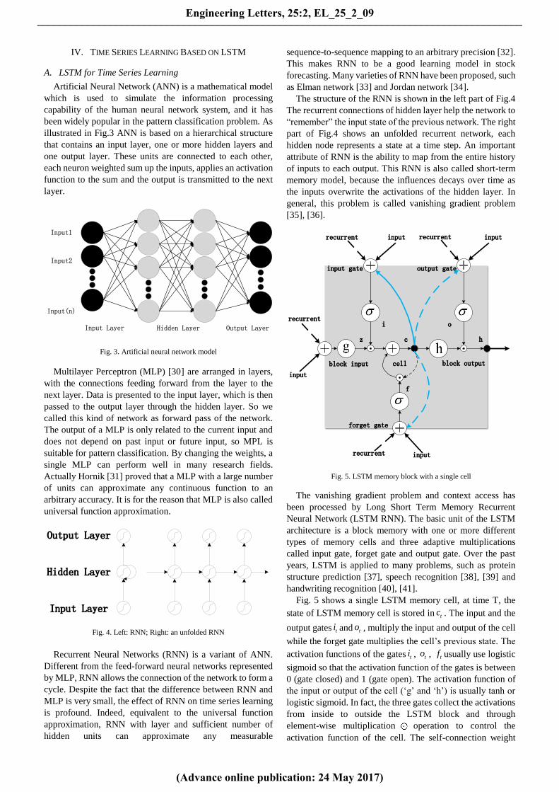
IV. TIME SERIES LEARNING BASED ON LSTM

A. LSTM for Time Series Learning

Artificial Neural Network (ANN) is a mathematical model

which is used to simulate the information processing

capability of the human neural network system, and it has

been widely popular in the pattern classification problem. As

illustrated in Fig.3 ANN is based on a hierarchical structure

that contains an input layer, one or more hidden layers and

one output layer. These units are connected to each other,

each neuron weighted sum up the inputs, applies an activation

function to the sum and the output is transmitted to the next

layer.

Input1

Input(n)

Input2

Input Layer Hidden Layer Output Layer

Fig. 3. Artificial neural network model

Multilayer Perceptron (MLP) [30] are arranged in layers,

with the connections feeding forward from the layer to the

next layer. Data is presented to the input layer, which is then

passed to the output layer through the hidden layer. So we

called this kind of network as forward pass of the network.

The output of a MLP is only related to the current input and

does not depend on past input or future input, so MPL is

suitable for pattern classification. By changing the weights, a

single MLP can perform well in many research fields.

Actually Hornik [31] proved that a MLP with a large number

of units can approximate any continuous function to an

arbitrary accuracy. It is for the reason that MLP is also called

universal function approximation.

Output Layer

Hidden Layer

Input Layer

Fig. 4. Left: RNN; Right: an unfolded RNN

Recurrent Neural Networks (RNN) is a variant of ANN.

Different from the feed-forward neural networks represented

by MLP, RNN allows the connection of the network to form a

cycle. Despite the fact that the difference between RNN and

MLP is very small, the effect of RNN on time series learning

is profound. Indeed, equivalent to the universal function

approximation, RNN with layer and sufficient number of

hidden units can approximate any measurable

sequence-to-sequence mapping to an arbitrary precision [32].

This makes RNN to be a good learning model in stock

forecasting. Many varieties of RNN have been proposed, such

as Elman network [33] and Jordan network [34].

The structure of the RNN is shown in the left part of Fig.4

The recurrent connections of hidden layer help the network to

“remember” the input state of the previous network. The right

part of Fig.4 shows an unfolded recurrent network, each

hidden node represents a state at a time step. An important

attribute of RNN is the ability to map from the entire history

of inputs to each output. This RNN is also called short-term

memory model, because the influences decays over time as

the inputs overwrite the activations of the hidden layer. In

general, this problem is called vanishing gradient problem

[35], [36].

cell

cz h

recurrent

recurrent recurrent

recurrent input

input

input

input

output gateinput gate

i o

block input block output

f

forget gate

Fig. 5. LSTM memory block with a single cell

The vanishing gradient problem and context access has

been processed by Long Short Term Memory Recurrent

Neural Network (LSTM RNN). The basic unit of the LSTM

architecture is a block memory with one or more different

types of memory cells and three adaptive multiplications

called input gate, forget gate and output gate. Over the past

years, LSTM is applied to many problems, such as protein

structure prediction [37], speech recognition [38], [39] and

handwriting recognition [40], [41].

Fig. 5 shows a single LSTM memory cell, at time T, the

state of LSTM memory cell is stored in tc . The input and the

output gates ti and to , multiply the input and output of the cell

while the forget gate multiplies the cell’s previous state. The

activation functions of the gates ti , to , tf usually use logistic

sigmoid so that the activation function of the gates is between

0 (gate closed) and 1 (gate open). The activation function of

the input or output of the cell (‘g’ and ‘h’) is usually tanh or

logistic sigmoid. In fact, the three gates collect the activations

from inside to outside the LSTM block and through

element-wise multiplication operation to control the

activation function of the cell. The self-connection weight



______________________________________________________________________________________

usually be 1, unless any outside interference, the state tc can

be constant from one time to another.

When a LSTM memory cell is at time t, the activation

function of the hidden layer is calculated as follows:

tx and th are the input and the output of LSTM block at

time t. zW , iW , fW and oW represent the input weight matrices

of the block input, input gate, forget gate and output gate,

zR , iR , fR and oR are the recurrent weight matrices of the

block input, input gate, forget gate and output gate.

ib , fb , cb and ob are the bias of the block input, input gate,

forget gate and output gate. represents element-wise

multiplication.

Block input: 1( )t z t z t zz g W x R h b (7)

Input gate: 1 1( )t i t i t i t ii W x R y p c b (8)

Forget gate: 1 1( )t f t f t f t ff W x R h p c b (9)

Cell state: 1t t t t tc i h f c (10)

Output gate: 1( )t o t o t o t oo W x R h p c b (11)

Block output: tanh( )t t th o c (12)

In fact, the role of the input gate is to control the input

signal that can change the state of the memory cell or block it.

The function of the output gate is to allow the state of memory

cell to have an effect on the other units or prevent it. The

forget gate is the self-connection of the memory cell so as to

let the cell remember or forget previous state. Due to the

multiplicative gates, LSTM can access more context

information than RNN, which alleviate the vanishing gradient

problem.

Hidden

Input

Output

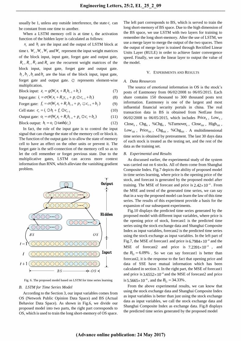
Fig. 6. The proposed model based on LSTM for time series learning

B. LSTM for Time Series Model

According to the Section 3, our input variables comes from

OS (Network Public Opinion Data Space) and BS (Actual

Behavior Data Space). As shown in Fig.6, we divide our

proposed model into two parts, the right part corresponds to

OS, which is used to train the long short-memory of OS space.

The left part corresponds to BS, which is served to train the

long short-memory of BS space. Due to the high dimension of

the BS space, we use LSTM with two layers for training to

remember the long short-memory. After the use of LSTM, we

use a merge layer to merge the output of the two spaces. Then

the output of merge layer is trained through Rectified Linear

Units Layer (RULE) in order to achieve faster convergence

speed. Finally, we use the linear layer to output the value of

the model.

V. EXPERIMENTS AND RESULTS

A. Data Resources

The source of emotional information in OS is the stock’s

posts of Eastmoney from 06/02/2008 to 06/05/2015. Each

share contains 150 thousand to 300 thousand posts text

information. Eastmoney is one of the largest and most

influential financial security portals in china. The real

transaction data in BS is obtained from NetEase from

06/02/2008 to 06/05/2015, which includes SPrice , SLow ,

SClose , SChg , S%Chg , S%Turnover , SHClose , SHHigh ,

SHLow , SHPrice , SHChg , SH%Chg . A multidimensional

time series is obtained by pretreatment. The last 30 days data

of each stock is treated as the testing set, and the rest of the

data as the training set.

B. Experimental and Results

As discussed earlier, the experimental study of the system

was carried out on 6 stocks. All of them come from Shanghai

Composite Index. Fig.7 depicts the ability of proposed model

in time series learning, where price is the opening price of the

stock, and forecast is generated by the proposed model after

training. The MSE of forecast and price is 42.42 10 . From

the MSE and trend of the generated time series, we can say

that in a way the proposed model can learn the law of this time

series. The results of this experiment provide a basis for the

expansion of our subsequent experiments.

Fig.10 displays the predicted time series generated by the

proposed model with different input variables, where price is

the opening price of stock, forecast1 is the predicted time

series using the stock exchange data and Shanghai Composite

Index as input variables, forecast2 is the predicted time series

using the stock exchange as input variables. In the left part of

Fig.7, the MSE of forecast1 and price is 46.7984 10 and the

MSE of forecast2 and price is 47.2391 10 , and

the 12 6.09%B . So we can say forecast1 is better than

forecast2, it is the response to the fact that opening price and

data of SSE have mutual information which has been

calculated in section 3. In the right part, the MSE of forecast1

and price is 43.6552 10 and the MSE of forecast2 and price

is 45.5665 10 , and the 12 34.33%B .

From the above experimental results, we can know that

using the stock exchange data and Shanghai Composite Index

as input variables is better than just using the stock exchange

data as input variables, we call the stock exchange data and

Shanghai Composite Index as exchange data. Fig.8 displays

the predicted time series generated by the proposed model



______________________________________________________________________________________

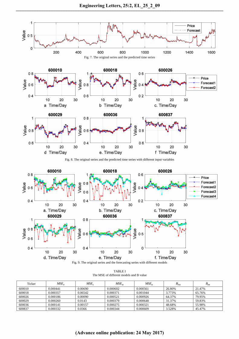
Fig. 7. The original series and the predicted time series

Fig. 8. The original series and the predicted time series with different input variables

Fig. 9. The original series and the forecasting series with different models

TABLE I

The MSE of different models and B value

Ticker PMSE SMSE

MMSE RMSE

PMB PRB

600010 0.000441 0.00690 0.000602 0.000561 26.80% 21.47%

600018 0.000357 0.06542 0.000371 0.001044 3.773% 65.76%

600026 0.000186 0.00090 0.000521 0.000926 64.37% 79.95%

600029 0.000260 0.0143 0.000379 0.000648 31.37% 59.83%

600036 0.000141 0.00157 0.000275 0.000321 48.68% 55.98%

600837 0.000332 0.0366 0.000344 0.000609 3.528% 45.47%



______________________________________________________________________________________

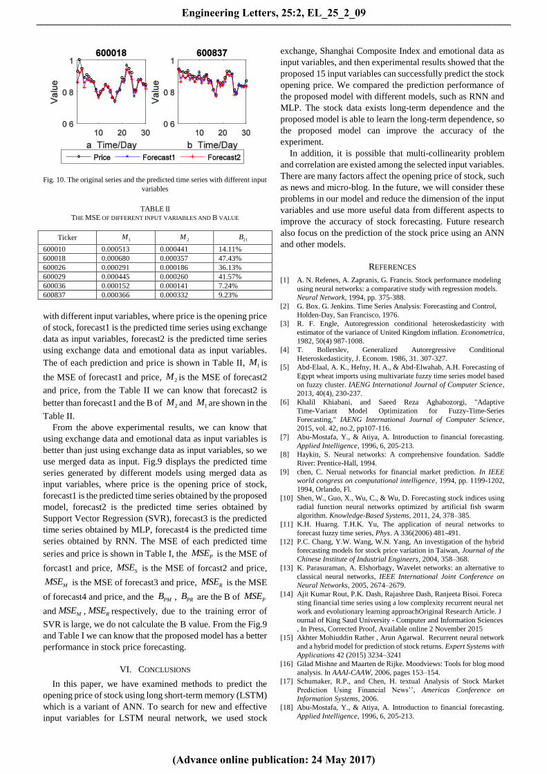
Fig. 10. The original series and the predicted time series with different input

variables

TABLE II

THE MSE OF DIFFERENT INPUT VARIABLES AND B VALUE

Ticker 1M 2M

21B

600010 0.000513 0.000441 14.11%

600018 0.000680 0.000357 47.43%

600026 0.000291 0.000186 36.13%

600029 0.000445 0.000260 41.57%

600036 0.000152 0.000141 7.24%

600837 0.000366 0.000332 9.23%

with different input variables, where price is the opening price

of stock, forecast1 is the predicted time series using exchange

data as input variables, forecast2 is the predicted time series

using exchange data and emotional data as input variables.

The of each prediction and price is shown in Table II, 1M is

the MSE of forecast1 and price, 2M is the MSE of forecast2

and price, from the Table II we can know that forecast2 is

better than forecast1 and the B of 2M and 1M are shown in the

Table II.

From the above experimental results, we can know that

using exchange data and emotional data as input variables is

better than just using exchange data as input variables, so we

use merged data as input. Fig.9 displays the predicted time

series generated by different models using merged data as

input variables, where price is the opening price of stock,

forecast1 is the predicted time series obtained by the proposed

model, forecast2 is the predicted time series obtained by

Support Vector Regression (SVR), forecast3 is the predicted

time series obtained by MLP, forecast4 is the predicted time

series obtained by RNN. The MSE of each predicted time

series and price is shown in Table I, the PMSE is the MSE of

forcast1 and price, SMSE is the MSE of forcast2 and price,

MMSE is the MSE of forecast3 and price, RMSE is the MSE

of forecast4 and price, and the PMB , PRB are the B of PMSE

and MMSE , RMSE respectively, due to the training error of

SVR is large, we do not calculate the B value. From the Fig.9

and Table I we can know that the proposed model has a better

performance in stock price forecasting.

VI. CONCLUSIONS

In this paper, we have examined methods to predict the

opening price of stock using long short-term memory (LSTM)

which is a variant of ANN. To search for new and effective

input variables for LSTM neural network, we used stock

exchange, Shanghai Composite Index and emotional data as

input variables, and then experimental results showed that the

proposed 15 input variables can successfully predict the stock

opening price. We compared the prediction performance of

the proposed model with different models, such as RNN and

MLP. The stock data exists long-term dependence and the

proposed model is able to learn the long-term dependence, so

the proposed model can improve the accuracy of the

experiment.

In addition, it is possible that multi-collinearity problem

and correlation are existed among the selected input variables.

There are many factors affect the opening price of stock, such

as news and micro-blog. In the future, we will consider these

problems in our model and reduce the dimension of the input

variables and use more useful data from different aspects to

improve the accuracy of stock forecasting. Future research

also focus on the prediction of the stock price using an ANN

and other models.

REFERENCES

[1] A. N. Refenes, A. Zapranis, G. Francis. Stock performance modeling

using neural networks: a comparative study with regression models.

Neural Network, 1994, pp. 375-388.

[2] G. Box. G. Jenkins. Time Series Analysis: Forecasting and Control,

Holden-Day, San Francisco, 1976.

[3] R. F. Engle, Autoregression conditional heteroskedasticity with

estimator of the variance of United Kingdom inflation. Econometrica,

1982, 50(4) 987-1008.

[4] T. Bollerslev, Generalized Autoregressive Conditional

Heteroskedasticity, J. Econom. 1986, 31. 307-327.

[5] Abd-Elaal, A. K., Hefny, H. A., & Abd-Elwahab, A.H. Forecasting of

Egypt wheat imports using multivariate fuzzy time series model based

on fuzzy cluster. IAENG International Journal of Computer Science,

2013, 40(4), 230-237.

[6] Khalil Khiabani, and Saeed Reza Aghabozorgi, "Adaptive

Time-Variant Model Optimization for Fuzzy-Time-Series

Forecasting," IAENG International Journal of Computer Science,

2015, vol. 42, no.2, pp107-116.

[7] Abu-Mostafa, Y., & Atiya, A. Introduction to financial forecasting.

Applied Intelligence, 1996, 6, 205-213.

[8] Haykin, S. Neural networks: A comprehensive foundation. Saddle

River: Prentice-Hall, 1994.

[9] chen, C. Nerual networks for financial market prediction. In IEEE

world congress on computational intelligence, 1994, pp. 1199-1202,

1994, Orlando, Fl.

[10] Shen, W., Guo, X., Wu, C., & Wu, D. Forecasting stock indices using

radial function neural networks optimized by artificial fish swarm

algorithm. Knowledge-Based Systems, 2011, 24, 378–385.

[11] K.H. Huarng. T.H.K. Yu, The application of neural networks to

forecast fuzzy time series, Phys. A 336(2006) 481-491.

[12] P.C. Chang, Y.W. Wang, W.N. Yang, An investigation of the hybrid

forecasting models for stock price variation in Taiwan, Journal of the

Chinese Institute of Industrial Engineers, 2004, 358–368.

[13] K. Parasuraman, A. Elshorbagy, Wavelet networks: an alternative to

classical neural networks, IEEE International Joint Conference on

Neural Networks, 2005, 2674–2679.

[14] Ajit Kumar Rout, P.K. Dash, Rajashree Dash, Ranjeeta Bisoi. Foreca

sting financial time series using a low complexity recurrent neural net

work and evolutionary learning approachOriginal Research Article. J

ournal of King Saud University - Computer and Information Sciences

, In Press, Corrected Proof, Available online 2 November 2015

[15] Akhter Mohiuddin Rather , Arun Agarwal. Recurrent neural network

and a hybrid model for prediction of stock returns. Expert Systems with

Applications 42 (2015) 3234–3241

[16] Gilad Mishne and Maarten de Rijke. Moodviews: Tools for blog mood

analysis. In AAAI-CAAW, 2006, pages 153–154.

[17] Schumaker, R.P., and Chen, H. textual Analysis of Stock Market

Prediction Using Financial News’’, Americas Conference on

Information Systems, 2006.

[18] Abu-Mostafa, Y., & Atiya, A. Introduction to financial forecasting.

Applied Intelligence, 1996, 6, 205-213.



______________________________________________________________________________________

[19] A.N. Refenes, A. Zapranis, G. Francis, Stock performance modeling

using neural networks: a comparative study with regression models,

Neural Networks, 1994, 375–388.

[20] Yoo, Y. n, G. Swales, T.M. Margavio, A comparison of discriminate

analysis versus artificial neural networks, Journal of the Operations

Research Society, 1993, 51–60.

[21] Wang, L., Zou, H., Su, J., Li, L., & Chaudhry, S. An ARIMA-ANN

hybrid model for time series forecasting. Systems Research and

Behavioral Science, 2013, 30, 244–259.

[22] Rout, M., Majhi, B., Majhi, R., & Panda, G. Forecasting of currency

exchange rates using an adaptive ARMA model with differential

evolution based training. Journal of King Saud University-Computer

and Information Sciences, 2014, 26, 7–18.

[23] Yi, X., Jin, X., John, L., & Shouyang, W. A multiscale modeling

approach incorporating ARIMA and ANNS for financial market

volatility forecasting. Journal of Systems Science and Complexity,

2014, 27, 225–236.

[24] Kim, K., & Ahn, H. Simultaneous optimization of artificial neural

networks for financial forecasting. Applied Intelligence, 2012, 36,

887–898.

[25] Chen, M., Fan, M., Chen, Y., & Wei, H. Design of experiments on

neural network’s parameters optimization for time series forecasting in

stock markets. Neural Network World, 2013, 23, 369–393.

[26] A.S. Chen, M.T. Leung, H. Daouk, Application of neural networks to

an emerging financial market: forecasting and trading the Taiwan

stock index, Computers and Operations Research, 2003, 901–923.

[27] K.H. Huarng. T.H.K. Yu, The application of neural networks to

forecast fuzzy time series, Phys. A 336 (2006) 481-491.

[28] Hsu, V. A hybrid procedure with feature selection for resolving

stock/futures price forecasting problems. Neural Computing and

Applications, 2013, 22, 651–671.

[29] Hsieh, T., Hsiao, H., & Yeh, W. Forecasting stock markets using

wavelet transforms and recurrent neural networks: An integrated

system based on artificial bee colony algorithm. Applied Soft

Computing, 2011, 11, 2510–2525.

[30] Rumelhart, G. E. Hinton, and R. J. Williams. Learning Internal

Representations by Error Propagation, pages 318-362. MIT Press,

1986.

[31] HORNIK, K., STINCHCOMBE, M., and WHITE, H., Multila y er F

eedforw ard Net w orks are Univ ersal Appro ximators, Neural

Networks, 1989, 2, pp. 359-366.

[32] Hammer. On the Approximation Capability of Recurrent Neural

Networks. Neurocomputing, 2000, 31(1-4):107-123.

[33] J. L. Elman. Finding Structure in Time. Cognitive Science, 1990

14:179–211.

[34] M. I. Jordan. Attractor dynamics and parallelism in a connectionist

sequential machine, 1990, pages 112–127. IEEE Press.

[35] Hochreiter. Unrersuchungen zu Dynamischen Neuronalen Netzen.

PhD thesis, Institut fur Informatik, Technische Universitat Munchen,

1991.

[36] Hochreiter, Y. Bengio, P. Frasconi, and J. Schmidhuber. Gradient Flow

in Recurrent Nets: the Difficulty of Learning Long-term Dependencies.

In S. C. Kermer and J. F. kolen, editors, A Field Guide to Dynamical

Recurrent Neural Networks. IEEE Press, 2001a.

[37] S. Hochreiter, M. Heusel, and K. Obermayer, “Fast model-based

protein homology detection without alignment,” Bioinformatics, 2007

vol. 23, no. 14, pp. 1728–1736.

[38] A. Graves and J. Schmidhuber, “Framewise phoneme classification

with bidirectional LSTM networks,” in Proceedings of the

International Joint Conference on Neural Networks, vol. 4. IEEE, 2005,

pp. 2047–2052.

[39] A. Graves, S. Fern andez, F. Gomez, and J. Schmidhuber,

“Connectionist temporal classification: Labelling unsegmented

sequence data with recurrent neural networks,” in Proceedings of the

23rd International Conference on Machine Learning. ACM, 2006, pp.

369–376.

[40] M. Liwicki, A. Graves, H. Bunke, and J. Schmidhuber, “A novel

approach to on-line handwriting recognition based on bidirectional

long short-term memory networks,” in Proceedings of 9th International

Conference on Document Analysis and Recognition, vol. 1, 2007, pp.

367–371.

[41] A. Graves, M. Liwicki, H. Bunke, J. Schmidhuber, and S. Fern andez,

“ Unconstrained on-line handwriting recognition with recurrent

neural networks,” in Advances in Neural Information Processing

Systems, 2008, pp. 577–584.

Qun Zhuge received his bachelor degree in College Mathematics and

Information Science, Wenzhou University. Now, he is a master degree

candidate of School of Computer Engineering and Science, Shanghai

University. His main research area is intelligent information processing.



______________________________________________________________________________________

lstm neural network with emotional analysis for prediction ... · stock opening price being the...

Documents