lssper: solving the resource-constrained project scheduling problem with large neighbourhood search

Annals of Operations Research 131, 237–257, 2004 2004 Kluwer Academic Publishers. Manufactured in The Netherlands.

LSSPER: Solving the Resource-Constrained ProjectScheduling Problem with Large Neighbourhood Search

MIREILLE PALPANT, CHRISTIAN ARTIGUES and PHILIPPE MICHELONLaboratoire d’Informatique d’Avignon, 339, chemin des meinajariès, Agroparc, BP 1228, 84911 AvignonCedex 9, France

Abstract. This paper presents the Local Search with SubProblem Exact Resolution (LSSPER) methodbased on large neighbourhood search for solving the resource-constrained project scheduling problem(RCPSP). At each step of the method, a subpart of the current solution is fixed while the other part de-fines a subproblem solved externally by a heuristic or an exact solution approach (using either constraintprogramming techniques or mathematical programming techniques). Hence, the method can be seen asa hybrid scheme. The key point of the method deals with the choice of the subproblem to be optimized.In this paper, we investigate the application of the method to the RCPSP. Several strategies for generat-ing the subproblem are proposed. In order to evaluate these strategies, and, also, to compare the wholemethod with current state-of-the-art heuristics, extensive numerical experiments have been performed. Theproposed method appears to be very efficient.

Keywords: resource-constrained project scheduling problem, large neighbourhood search

1. Introduction

The problem of searching a given neighbourhood of an NP-hard problem can be itselfdefined as a combinatorial optimization problem. In this paper we consider the neigh-bourhood of a solution to an n variables NP-hard problem P as the set of solutions toa p variables subproblem obtained directly from P by fixing n − p variables to theircurrent value. With no restrictive assumption on p, finding the best neighbour is likelyto be itself an NP-hard problem and the number of neighbours is exponential in p.

When p is small enough, an exhaustive enumeration of the neighbours can beperformed but the so-defined neighbourhood is unlikely to contain interesting feasiblesolutions. In this paper we consider larger values of p, presumably defining a (very)large neighbourhood, and we search for the best neighbour with an implicit enumerationtechnique or a heuristic.

Successful applications of large neighbourhood search (LNS) are available in theliterature for various problems. For the quadratic assignment problem (QAP), the MI-MAUSA method designed by Mautor and Michelon (1997) builds at each iteration a re-duced QAP and solves it by branch and bound. For the vehicle routing problem (VRP),Shaw (1998), Gendreau, Pesant, and Rousseau (2002), and recently Bent and Henten-ryck (2001), consider the removal of several customer visits and re-insert them by usinglimited discrepancy search (LDS). The latter succeeds in improving best published so-lutions of standard VRP instances with time windows. In (Taillard and Voss, 2002),

238 PALPANT, ARTIGUES AND MICHELON

Taillard and Voss propose a general algorithm (POPMUSIC) in which subproblems arebuilt from subparts of the solution. A survey of very large scale neighbourhood searchtechniques can be found in (Ahuja et al., 2002).

In this paper, we consider the resource-constrained project scheduling problem(RCPSP) in which a set of activities has to be scheduled, subject to precedence con-straints and resource limitations with the objective to minimise the total project durationor makespan. This problem has received special attention in the last decades because ofits relative generality and its numerous practical applications (see (Brucker et al., 1999;Kolisch and Padman, 2001) for recent surveys). Furthermore it is particularly hard to at-tack. Thus, the best exact methods proposed so far are unable to solve some benchmarkinstances consisting of 60 activities and 4 resources.

The use of LNS for solving scheduling problems is not new. Indeed, the shift-ing bottleneck heuristic, initially designed by Adams, Balas, and Zawack (1988), isone of the most popular heuristics to solve the famous job-shop problem (JSP) andsome of its extensions including multiresource operations, multipurpose machines, setuptimes and deadlines (see for instance (Balas et al., 1998; Schutten, 1998)). In the shift-ing bottleneck heuristic, the neighbourhood is defined by deriving a one-machine sub-problem from the current solution. The best neighbour is then found by solving thisproblem exactly. For the classical JSP, other LNS heuristics using various subproblemgeneration and resolution schemes have been proposed in (Applegate and Cook, 1991;Baptiste, Le Pape, and Nuijten, 1995; Caseau and Laburthe, 1999). The latter approachis the forget-and-extend heuristic of Caseau and Laburthe which has obtained excel-lent results on hard job-shop instances. The neighbourhood is defined by keeping theprocessing order of operations, either belonging to a variable set of resources (as for theshuffling procedure of Applegate and Cook (1991)), or scheduled in a variable temporalslice. Hence different neighbourhood types are considered for diversification purposes.The corresponding subproblems are solved by LDS combined with the powerful con-straint propagation “shaving” technique. Some LNS methods have also been proposedrecently for other scheduling problems such as the single machine total weighed tardi-ness (Congram, Potts, and Van de Velde, 2002), parallel machines (Frangioni, Scutellà,and Necciari, 2004) and unrelated machines (Sourd, 2001) problems.

Despite the success of LNS methods for (job-shop) scheduling, to the best of ourknowledge no heuristic of this type for the RCPSP has been proposed yet though it isan extension of the JSP. To fill this gap, we propose in this paper a new LNS methodfor the RCPSP. This method differs from the ones cited above by the way it explores theneighbourhood. Indeed, we concentrate our efforts on the generation of the subproblem,leaving its resolution to a commercial solver. The size of the subproblem self-adapts tothe time spent by the solver to provide the solution. These features give our method apractical interest since it is designed with almost no assumption on the method used toexplore the neighbourhood.

In section 2, we briefly describe the principles of the used LNS method in a generalcontext. In section 3, we propose a solution approach for the RCPSP based on the LNS

LSSPER 239

method. In section 4, we conclude by discussing the computational results obtained onstandard benchmark instances.

2. General description of the method

Let us consider the resolution of a general optimisation problem

P : minX∈X

f (X), with X = (x1, . . . , xn).

Throughout the paper, a capital letter (e.g., X) denotes a vector of decision variableswhereas an overline capital letter (e.g., X) represents a vector of values of the corre-sponding variables.

The proposed LNS metaheuristic is widely inspired by the MIMAUSA method ofMautor and Michelon (1997, 2001). It aims at alternating intensification and diversifica-tion phases (Glover and Laguna, 1997) in the search of solutions.

Intensification phases consist of exploring deeply a given subset of the feasibleregion X by solving successive subproblems. Thus, at each iteration s, a subproblem �s

of size p is generated by fixing n −p variables to the value they have in current solution

Xs−1

to P . Solving �s generates a solution Ys

whose extension to global problem P

provides the neighbour solution Xs

of Xs−1

.Conversely, diversification aims at visiting a subset of the feasible region X which

has not been explored yet. It consists in applying a diversification operator to the currentsolution.

The method, which returns final solution X∗, is detailed in figure 1.

Step 1 is assumed to compute (quickly) a feasible solution X0

to P using anyproblem-dependent heuristic. The other major points of the algorithm are developed inthe subsequent subsections:

• the subproblem generation and the auto-adjustment of its size are described in sec-tion 2.1,

• subproblem resolution strategies are discussed in section 2.2,

• the generation of neighbours and additional diversification procedures are presentedin section 2.3.

2.1. A self-adapting subproblem construction

At each iteration s, a subproblem of varying size p

�s: minY∈Y

g(Y ), with Y = (y1, . . . , yp),

is constructed by using problem P and its current solution Xs−1

. Roughly, the construc-tion method consists in selecting p � n variables xi1 , . . . , xip (renamed y1, . . . , yp) of


Begin

1. Compute an initial solution X0

to problem P

2. Set X∗

:= X0, s := 1

3. Initialise p

4. Repeat

5. Generate a subproblem �s of size p using P and its current solution Xs−1

6. Solve �s within a maximum time limit H and store actual resolution time t s

7. If a solution Ys

to �s is obtained then8. Compute new solution X

sby extending Y

s

9. Else

10. Set Xs

:= Xs−1

11. End If12. If f (X

s) < f (X

∗) then

13. Set X∗

:= Xs

14. End If15. If the diversification condition is verified then16. Modify X

sby a diversification operator

17. End If18. Adjust p by using statistics on t s, . . . , t s−q

19. s := s + 120. Until stop criterion is metEnd

Figure 1. General algorithm of the proposed method.

P and in replacing in the constraints of P the n − p remaining variables xip+1 , . . . , xin

by their current values xip+1 , . . . , xin .Any feasible solution Y of subproblem �s has to be such that Z verifying zi1 =

y1, . . . , zip = yp and zip+1 = xip+1 , . . . , zin = xin is a feasible solution of P . Let Y∗

denote the optimal solution of �s and let Z∗

denote the corresponding extension to P .Objective function g is such that f (Z

∗) � f (X).

A stronger alternative consists of considering additional constraints such that forany feasible solution Y of subproblem �s , f (Z) � f (X). In such a case, any feasible

solution of subproblem �s can be obviously extended to obtain a neighbour Xs

of Xs−1

for problem P verifying f (Xs) � f (X

s−1).

The auto-adjustment of size p is related to statistics on q consecutive values oft s , . . . , t s−q, q � 1, where t s denotes the time spent at iteration s to solve subproblem�s . If t s tends to increase, then p is decreased, until a lower bound p is reached. If t s

tends to decrease, the size of the subproblem is increased, until p = n.Once p is determined, the selection of the p variables results from a problem-

dependent analysis of the constraints of P with the objective to ensure that:

LSSPER 241

• the neighbourhood defined by �s has a “reasonable” size, i.e. contains a large numberof solutions that can be explored by an implicit enumeration method or a heuristic,

• the neighbourhood defined by �s contains promising solutions,

• the feasible region X of P is sufficiently explored by solving consecutive subprob-lems �q , q � 1 (diversification of the search): the p variables must be selected in anon-uniform way.

2.2. Resolution of the subproblem and intensification of the search

Once defined, an attempt to solve the subproblem �s is performed within a maximalallotted time H . We assume the resolution method to be any (external to our method)exact or approximate solution approach for problem �s . If feasible (possibly optimal)solution Y

sto �s is found then the time t s � H spent to obtain it is stored. Otherwise,

t s is set to an arbitrary large value. A large time limit H corresponds to an intensificationof the search since more time is spent in the search of the best solution of �s , i.e. thebest neighbour, and is more likely coupled with the use of an exact method. Conversely,setting H to a small value aims at finding (hopefully) quickly a feasible solution of �s .

2.3. Generation of the neighbour solution and additional diversification of the search

Once a solution Ys

to problem �s has been obtained, solution Xs

has to be generated

by extending Ys

to problem P . The simplest way consists in replacing in Xs−1

valuesxi1 , . . . , xip by values y1, . . . , yp. In practice, some additional improvements can beperformed depending on the problem structure.

Although the varying size of the subproblem and its non-uniform generationscheme bring some diversification to the search, additional diversification procedurescan be used to explore other solution subspaces. These can consist of increasing consid-erably the subproblem size, accepting non improving neighbours, rebuilding new solu-tions from scratch, etc.

3. Application to the resource-constrained project scheduling problem

In this section, we adapt the method presented in section 2 for the resource-constrainedproject scheduling problem. A formulation of this problem is given in section 3.1. In sec-tion 3.2, we give a brief overview of schedule generation schemes, heuristics and meta-heuristics proposed in the literature for the RCPSP. Then, we detail the implementationof the proposed method. The initial solution generation method is given in section 3.3.The subproblem generation and resolution procedures are presented in sections 3.4 and3.5, respectively. Finally, the neighbour generation and the additional diversificationprocedures are described in section 3.6.


3.1. Problem description

In the resource-constrained project scheduling problem, A = {1, . . . , n} denotes the setof activities and R = {1, . . . , m} denotes the set of resources. Each resource k ∈ R

has a limited availability Rk. Each activity i ∈ A has a duration pi � 0 and a requestrik � 0 on each resource k ∈ R. The activities are organised in a project representedby an activity-on-node graph (also called project network) G = {V,E}, where V =A∪{0, n+1} is the set of nodes representing the activities and E is the set of directed arcsrepresenting the precedence constraints. A directed arc (i, j) ∈ E means that activity i

must be completed when activity j starts. 0 and n+ 1 are dummy activities representingthe start and the end of the schedule, respectively. Their processing times and requestsare all set to 0. Node 0 is connected to any activity without predecessor and node n + 1is connected to any activity without successor. The variables of the problem being thestarting times S = (S1, . . . , Sn+1), the RCPSP can be formulated as follows:

(P ) min Sn+1 (1)

Sj � Si + pi ∀(i, j) ∈ E, (2)∑i∈A(τ,S)

rik � Rk ∀k ∈ R,∀τ ∈ {0, . . . , UB} (3)

where S0 = 0 and A(τ, S) is the set of activities in process at time τ in solution S, i.e.verifying Si � τ < Si + pi .

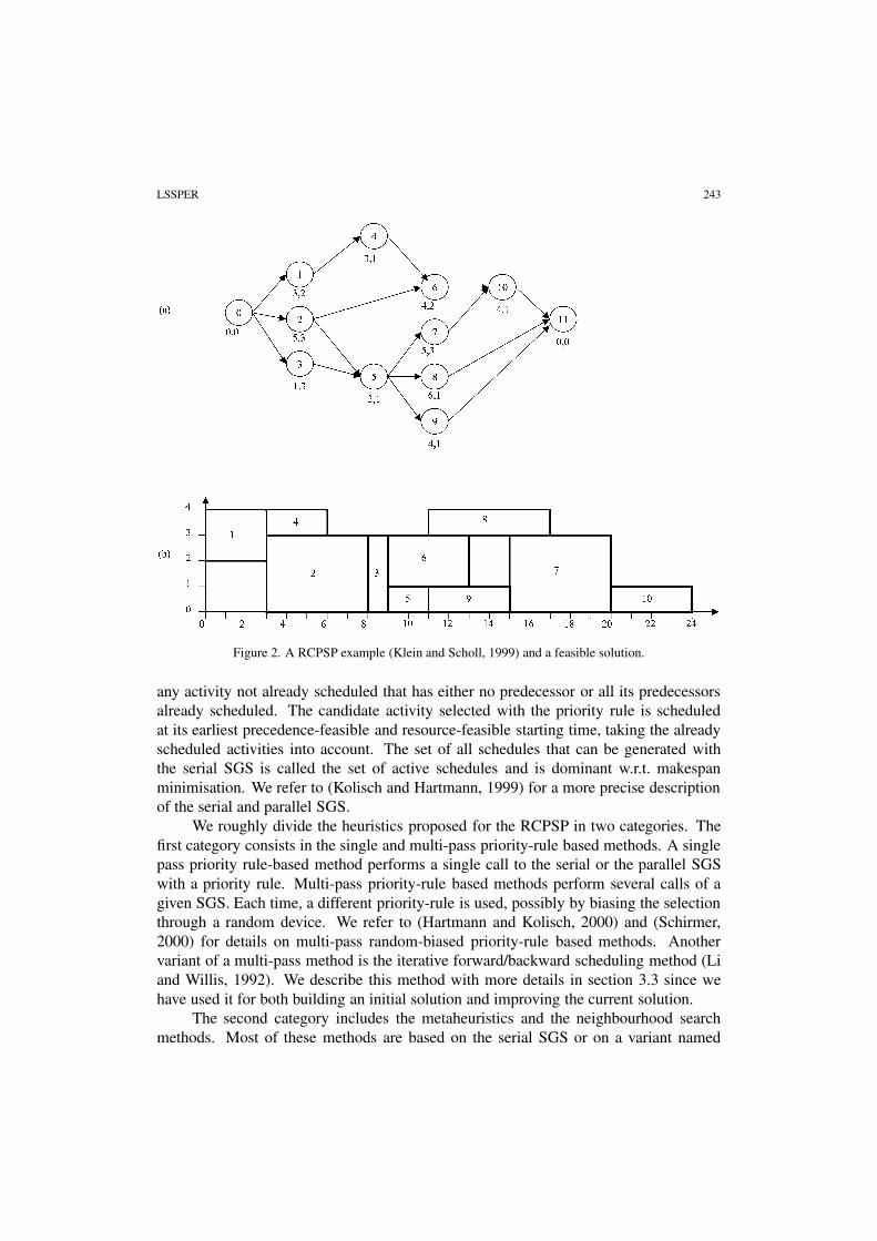
This problem is strongly NP-hard, as an extension of the job-shop problem. Fig-ure 2 displays an example taken from (Klein and Scholl, 1999) with 10 non-dummyactivities and a single resource of 4 units. In part (a) of the figure, the project network isdisplayed. Under each node, the duration and the request of the corresponding activityare given, respectively. In part (b) of the figure, a feasible schedule of makespan 24 isrepresented by way of an extended Gantt chart.

3.2. Schedule generation schemes, metaheuristics and neighbourhoods for the RCPSP

In this section we first give a short overview of the constructive heuristics designed forthe RCPSP. Then, we discuss the different neighbourhoods that have been used so far forthis problem. For a recent state-of-the-art review of heuristics for the RCPSP we refer to(Hartmann and Kolisch, 2000).

The simplest heuristics are constructive. They build a feasible solution startingfrom scratch. A constructive heuristic has generally n steps, where n denotes the num-ber of activities. At each step, a single activity is selected for being scheduled among aset of candidate activities. The way this set is generated and the scheduling process ofthe selected activity are both determined by a schedule generation scheme (SGS). A pri-ority rule generally determines which activity is selected for being scheduled among thecandidate ones.

Two SGS are commonly used in the literature: the parallel SGS and the serialSGS. The serial SGS, used in the present study, puts in the set of candidate activities

LSSPER 243

Figure 2. A RCPSP example (Klein and Scholl, 1999) and a feasible solution.

any activity not already scheduled that has either no predecessor or all its predecessorsalready scheduled. The candidate activity selected with the priority rule is scheduledat its earliest precedence-feasible and resource-feasible starting time, taking the alreadyscheduled activities into account. The set of all schedules that can be generated withthe serial SGS is called the set of active schedules and is dominant w.r.t. makespanminimisation. We refer to (Kolisch and Hartmann, 1999) for a more precise descriptionof the serial and parallel SGS.

We roughly divide the heuristics proposed for the RCPSP in two categories. Thefirst category consists in the single and multi-pass priority-rule based methods. A singlepass priority rule-based method performs a single call to the serial or the parallel SGSwith a priority rule. Multi-pass priority-rule based methods perform several calls of agiven SGS. Each time, a different priority-rule is used, possibly by biasing the selectionthrough a random device. We refer to (Hartmann and Kolisch, 2000) and (Schirmer,2000) for details on multi-pass random-biased priority-rule based methods. Anothervariant of a multi-pass method is the iterative forward/backward scheduling method (Liand Willis, 1992). We describe this method with more details in section 3.3 since wehave used it for both building an initial solution and improving the current solution.

The second category includes the metaheuristics and the neighbourhood searchmethods. Most of these methods are based on the serial SGS or on a variant named


the “list scheduling algorithm” (Kolisch and Hartmann, 1999; Hartmann and Kolisch,2000). Thanks to the dominance property of the set of active schedules, there existsan input priority vector (or an input list L∗ for the variant) of the serial SGS leadingto the optimal schedule. Most of the metaheuristics proposed for the RCPSP (some ofthem being evaluated in (Hartmann and Kolisch, 2000)) take advantage of this prop-erty and restrict the search to priority vectors or to feasible lists. This is for examplethe case of simulated annealing approaches (Lee and Kim, 1996; Cho and Kim, 1997;Bouleimen and Lecocq, 2003), genetic algorithms (Leon and Ramamoorthy, 1995;Lee and Kim, 1996; Hartmann, 1998; Kohlmorgen, Schmeck, and Haase, 1999),tabu search (Pinson, Prins, and Rullier, 1994; Baar, Brucker, and Knust, 1998; Valls,Ballestin, and Quintanilla, 2000; Nonobe and Ibaraki, 1999; Thomas and Salhi, 1998),best fit search (Naphade, Wu, and Storer, 1997), ant colony algorithm (Merkle, Midden-dorf, and Schmeck, 2002). In these approaches, a move computes a neighbour activitylist or a neighbour priority vector. However, it has to be pointed out that for the activitylist as well as for the priority vector representation, the number of neighbour activity lists(or priority vectors) does not necessary reflect the number of actual neighbour solutionsin terms of activity starting times. Indeed, it is well known that several different lists orpriority vectors can lead to the same solution.

Other neighbourhood search methods based on different schedule representationshave been proposed, like the shift vector representation (Sampson and Weiss, 1993),the schedule scheme representation (Baar, Brucker, and Knust, 1998), the disjunctivearc based representation (Bell and Han, 1991) and the activity-on-node/network flowrepresentation (Artigues, Michelon, and Reusser, 2003).

In contrast with these approaches, we focus in this paper on the direct representa-tion of the schedule by the vector of starting times. Indeed, as it will be presented in thenext subsections, this allows to define the search for the best neighbour as a schedulingsubproblem. In this framework, an interesting approach has been used in (Mausser andLawrence, 1997), where the makespan of a given solution is improved by reschedul-ing entirely at each step a block of activities. A block is composed by the activitiesentirely scheduled in a given time slice, as in the Forget and Extend heuristic (Caseauand Laburthe, 1999). The rescheduling of a given block potentially represents a largeneighbourhood. Hence, such a block structure is considered in the present study.

3.3. Generation of an initial solution

In this subsection, we describe how we generate an initial solution S0

for our imple-

mentation of LNS for the RCPSP. S0

is generated with a variant of the iterative for-ward/backward heuristic (Li and Willis, 1992). This heuristic alternates forward andbackward passes of the serial SGS, computing each time a feasible schedule. The for-ward pass computes a solution by applying the serial SGS to the RCPSP problem P ,whereas the backward pass computes a solution by considering its “mirror” problemMP obtained by reversing all arcs of the project network. In our variant, we ensure thateach generated schedule has a makespan non-greater than the previous one, thanks to

LSSPER 245

the selected priority rules. This property together with the stop condition ensures a fastconvergence.

In the first forward pass, we generate a schedule with the serial SGS and theMINLFT priority rule.1 Then we apply iteratively backward and forward passes un-der the following scheme. Let FS (FF) be the start (finish) time vector computed by

the forward pass. We set S0 := FS. The backward pass consists in applying the serial

SGS to MP, by taking as priority vector, FFn+1 − FF. Let BS (BF) be the start (fin-ish) time vector computed by the backward pass. It can be easily shown that we can

set S0 := BF − BF0 without increasing the makespan. Indeed, such a backward pass

amounts to applying a right shift to each activity in the solution FS, in the non increas-ing order of the completion times FF, the right shift being bounded from above by thecurrent makespan.

If the makespan has not been decreased, the process stops. Otherwise, the next for-ward pass consists in applying the serial SGS to P , by taking the new current start time

vector S0

as priority vector. Again, the obtained start time vector FS verifies FSn+1 � S0.

The process iterates until two consecutive forward and backward passes obtain the samemakespan.

3.4. Generation of the subproblem

In contrast with most of the state-of-the-art methods, we do not use any special solu-tion representation such as activity lists, priority vectors or disjunctive graphs. Hencea solution is only represented in terms of a precedence- and resource-feasible start timevector S.

At each iteration s � 1 of the method, the subproblem �s and, consequently, theneighbourhood are defined by a set As ⊆ A of p activities As = {i1, . . . , ip} excludingdummy activities 0 and n+1. Once these p activities have been selected, the subproblem�s can be stated as follows. Each activity j ∈ A \ As being “frozen” at its current start

time value Ss−1j , find a feasible schedule minimising the makespan of the remaining

activities.In practice, freezing the start time of some activities is equivalent to generate a new

RCPSP applying the 3 following steps:

• We build a reduced project network Gs = (As, Es) including only the non-frozenactivities where Es = {(i, j) | i, j ∈ As, (i, j) ∈ E}.

• We modify the resource set R such that the availability Rkτ of each resource k ∈ R

at time period τ reflects the possibly frozen activities in process during τ :

Rkτ = Rk −∑

j∈(A\As)∩A(τ,Ss−1

)

rjk.

• For each activity i ∈ As , we compute recursively a time window [ESi , LSi] by takingthe predecessor(s) and successor(s) of i as well as resource availability into account.


First, we compute earliest and latest start times taking into account precedence con-straints of both frozen and selected activities:

ESpred

i = max{

maxj∈A\As,(j,i)∈E

Ss−1j + pj , max

j∈As,(j,i)∈EsESj + pj

},

LSsucci = min

{min

j∈A\As,(i,j)∈ES

s−1j − pi, min

j∈As,(i,j)∈EsLSj − pi

}.

As it can be seen in the computation of LSsucci , we also force any activity to be com-

pleted at the current makespan value Ss−1n+1.

Second, we right (resp. left) shift the earliest (resp. latest) start time until the activitycan be processed without interruption w.r.t. resource availability:

ESi = min{t | t � ESpred

i ,∀k ∈ R,∀τ = t, . . . , t + pi − 1, Rkτ � rik

},

LSi = max{t | t � LSsucc

i ,∀k ∈ R,∀τ = t, . . . , t + pi − 1, Rkτ � rik

}.

The variables of the subproblem built at iteration s being the starting times(Ss

i1, . . . , Ss

ip), �s can be formulated as follows:

(�s) mini∈As {max Ssi } (4)

Ssi � ESi ∀i ∈ As, (5)

Ssi � LSi ∀i ∈ As, (6)

Ssj � Ss

i + pi ∀(i, j) ∈ Es, (7)∑

i∈As∩A(τ,Ss)

rik � Rkτ ∀k ∈ R,∀τ ∈ {0, . . . , S

s−1n+1

}. (8)

The subproblem �s can be defined as a RCPSP with time windows and varyingresource availability, which makes it in a sense more general than the original problem!It is also easy to verify that any feasible solution of the subproblem can lead to a feasible

new solution Ss

of (P ) by setting Ss

i = Ss−1i ∀i ∈ A \ As . However, S

s

n+1 may bedifferent from objective function value (4). We will see in section 3.6 how neighboursolution S

sis further improved.

In figure 3, the subproblem generation is applied on the current solution of theillustrative example displayed in figure 2, assuming that p is set to 4 and that activitiesAs = {7, 8, 9, 10} have been selected. In part (a) of the figure, the selected activitiesare displayed. Part (b) of the figure displays the computed time windows. Part (c) ofthe figure shows the resource profile after removing the units required by the frozenactivities. Last, part (d) of the figure displays the project network of the subproblem.

We now explain how to determine the number p of activities constituting the sub-problem �s and how the p activities are selected.

As mentioned in section 2.1, the computation of p self-adapts in function of thetime spent to solve the subproblem at the previous iterations. Let H denote the maximumCPU time allotted to the subproblem resolution method. Let t s−1 be the time spent tosolve the subproblem at iteration s − 1. Let t = ∑

q=s−1,...,s−5 tq the total time spent

LSSPER 247

Figure 3. Example of subproblem generation with p = 4.

on the subproblem resolution over the last 5 iterations. We have used the followingempirical rules. If t � H then we set p := p + 2. If H < t � 5H/2 then we setp := p + 1. If 5H/2 < t � 4H then we set p := p − 1. If 4H < t � 5H then we setp := p − 2. No decrease on p is made if a given lower bound p is reached.

To select the p activities, i.e. to build the set As , we have compared in our experi-ments the 5 following possibilities (see section 4):

1. Critical&Random. The p activities are selected randomly but a higher probability isassigned to critical activities. We decide that an activity is critical when it has beenscheduled at the same start times on the last two passes of the forward/backwardmethod.


2. Random&Project Predecessors. The p activities are selected randomly but each timean activity is selected, its immediate predecessor(s) in the project network is (are)also selected.

3. Random&Contiguous Predecessors. The p activities are selected randomly but each

time an activity i is selected, any activity verifying Ss−1j + pj = S

s−1i is selected.

4. Random&All Predecessors. The p activities are selected by combining 2 and 3.

5. Block. A single activity i is randomly selected and included in As . Then, each activity

j contiguous to i or scheduled in parallel with i, (i.e. verifying Ss−1i − pj � S

s−1j �

Si + pi) is included in As in the limit of p activities. If this limit is not reached, weiterate the process from the second, third, . . . , activity added to As . For diversificationpurpose, the activities are considered for being included in As in a predefined randomorder.

For selection methods 2–5, the objective is to generate subproblems having sufficientindependence with the rest of the solutions to make the represented neighbourhood largeenough. Selection scheme 5 can be seen as an adaptation of the methods proposed in(Caseau and Laburthe, 1999; Mausser and Lawrence, 1997). The subproblem displayedin figure 3 is obtained by selection scheme 5, p = 4 and a random selection of activity 7.

The only 3 activities verifying the condition Ss−17 −pj � S

s−1j � S

s−17 + p7 are 8, 9 and

10. Hence any selection order would have lead to this subset of activities for p = 4.

3.5. Solving the subproblem

Our approach consists in evaluating the generality of the proposed method and its ap-plicability in practical situations by leaving the subproblem resolution to a commercialsolver. In our experiments, we have used a constraint programming solver specialized inscheduling and an integer linear programming solver. For the CP solver, constraints aredirectly written since a library of scheduling constraints is available. For the ILP solver,we use an extension of the well-known ILP formulation of Pritsker, Waters, and Wolfe(1969) to time windows and time-varying resource availability. In the model of Pritsker,Waters, and Wolfe, decision variables are the 0–1 variables xiτ = 1 if and only if activityi starts at time τ . In particular, there is a resource constraint per resource and per periodswhich makes easy the extension of the model to non-constant resource availability. Inboth cases, no particular tuning is performed (see section 4). The solver is allotted H

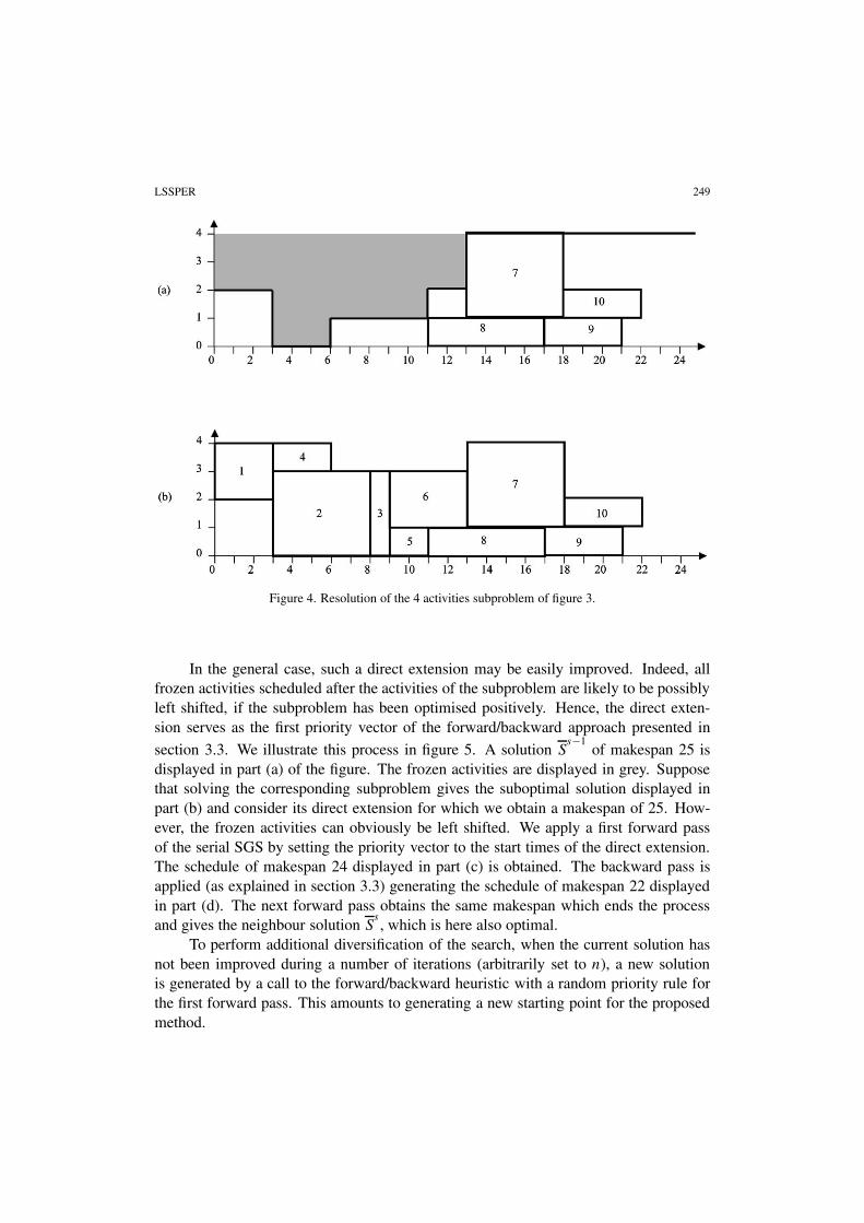
time units and it returns the best solution found (if any) during this time limit.In figure 4 we give in part (b) an example of solution S

sobtained by a direct

extension of the solution returned by the solver (part (a)) for the subproblem of figure 3.In this case, an improved (and optimal) solution of makespan 22 is obtained.

3.6. Neighbour generation and additional diversification

At iteration s, a feasible neighbour solution Ss

of Ss−1

is directly obtained by extendingthe subproblem solution (see section 3.4).

LSSPER 249

Figure 4. Resolution of the 4 activities subproblem of figure 3.

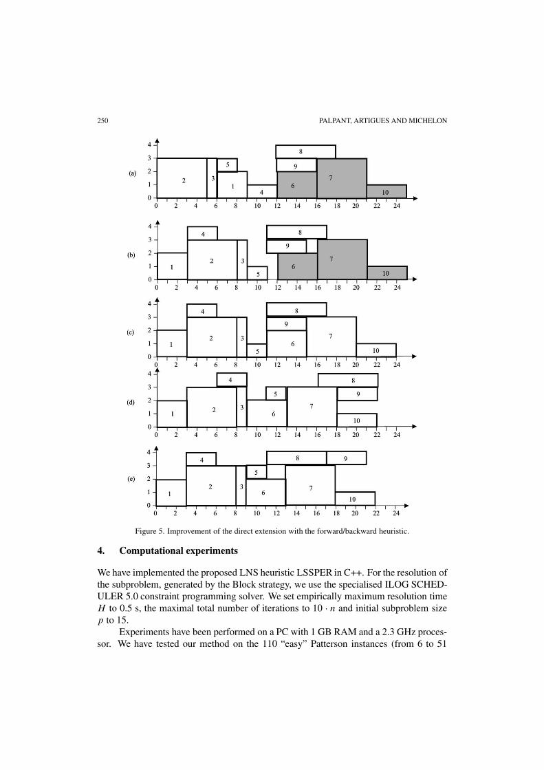
In the general case, such a direct extension may be easily improved. Indeed, allfrozen activities scheduled after the activities of the subproblem are likely to be possiblyleft shifted, if the subproblem has been optimised positively. Hence, the direct exten-sion serves as the first priority vector of the forward/backward approach presented in

section 3.3. We illustrate this process in figure 5. A solution Ss−1

of makespan 25 isdisplayed in part (a) of the figure. The frozen activities are displayed in grey. Supposethat solving the corresponding subproblem gives the suboptimal solution displayed inpart (b) and consider its direct extension for which we obtain a makespan of 25. How-ever, the frozen activities can obviously be left shifted. We apply a first forward passof the serial SGS by setting the priority vector to the start times of the direct extension.The schedule of makespan 24 displayed in part (c) is obtained. The backward pass isapplied (as explained in section 3.3) generating the schedule of makespan 22 displayedin part (d). The next forward pass obtains the same makespan which ends the processand gives the neighbour solution S

s, which is here also optimal.

To perform additional diversification of the search, when the current solution hasnot been improved during a number of iterations (arbitrarily set to n), a new solutionis generated by a call to the forward/backward heuristic with a random priority rule forthe first forward pass. This amounts to generating a new starting point for the proposedmethod.


Figure 5. Improvement of the direct extension with the forward/backward heuristic.

4. Computational experiments

We have implemented the proposed LNS heuristic LSSPER in C++. For the resolution ofthe subproblem, generated by the Block strategy, we use the specialised ILOG SCHED-ULER 5.0 constraint programming solver. We set empirically maximum resolution timeH to 0.5 s, the maximal total number of iterations to 10 · n and initial subproblem sizep to 15.

Experiments have been performed on a PC with 1 GB RAM and a 2.3 GHz proces-sor. We have tested our method on the 110 “easy” Patterson instances (from 6 to 51

LSSPER 251

Table 1Best results of the proposed LNS Search.

Prob. av. (max) �UB av. �LB # best av. (max) CPU av. (max) # sched

PAT 0 (0) – 110/110 1.60 (59) –ALV −0.46 (5.19) 46.24 45/48 232.23 (498) –BL 0.11 (4.17) – 38/39 17.61 (66) –

KSD30 0 (0) – 480/480 10.26 (123) 830 (1120)KSD60 0.22 (3.54) 10.81 413/480 38.78 (223) 1622 (2262)KSD90 0.40 (5.65) 10.29 379/480 61.25 (309) 2441 (3488)

KSD120 1.51 (20.91) 32.41 241/600 207.93 (501) 3396 (5000)

activities) (Patterson, 1984) (PAT), the 39 highly cumulative Baptiste/Le Pape instanceswith 20 activities (Baptiste and Le Pape, 2000) (BL), the 48 Alvarez instances with 103activities (Alvarez-Valdés and Tamarit, 1989) (ALV) and the 2040 Kolisch et al. in-stances with 30, 60, 90 and 120 activities (Kolisch, Sprecher, and Drexl, 1998) (KSD).

Our results are displayed in table 1. For each problem set, we display in the first twocolumns the average/maximal deviation from the optimum or from the best known upperbound and the average deviation from the critical path lower bound for the problemswhose optimal makespans are still unknown. The number of times we obtain the bestsolution, the average/maximal CPU time required and the average/maximal number ofgenerated schedules are indicated in the next columns. This latter value corresponds tothe total number of schedules generated by our method for the resolution of an instance.It sums the number of solutions found by the solver during the subproblem resolutionand the number of schedules computed by the forward/backward heuristic.

For all instances, except for KSD 120 set, the solutions found by LSSPER are onaverage within 0.5% above the best known solutions. At the time of the experiments,we have found new best solutions on the KSD and ALV sets. We still have 14, 9 and 4best known solutions for the KSD 60, 90 and 120 sets,2 respectively. We have solved tooptimality all the Baptiste/Le Pape instances except one. However we need twice moreCPU time to solve these 20 activities instances than for the 30 activities KSD instances.This seems to confirm the hardness of these highly cumulative instances (Baptiste andLe Pape, 2000) whereas some (but not all!) KSD instances are very easy.

To further analyse our results we compare them with current best state-of-the-artheuristics, all limited to 5000 generated schedules, on the KSD instances: the hybridgenetic algorithm of Valls, Ballestin, and Quintanilla (2002), the self-adapting geneticalgorithm of Hartmann (1998), the tabu search method of Nonobe and Ibaraki (1999), thesimulated annealing of Bouleimen and Lecocq (2003) and the random biased samplingmethod of Kolish (1996). Table 2 displays for each method the average deviation abovethe optimum (KSD30) or CPM lower bound (KSD 60, 90, 120).

The results show that our approach is very competitive with the approaches en-countered in the literature. The results on the KSD instances are better than the ones ofall the methods presented here. As for these approaches, the average number of gener-ated schedules does not exceed 5000. However, this has to be tempered by the possibly


Table 2Comparison with state-of-the-art approaches.

Method av. �UB av. �LB av. �LB av. �LB(KSD30) (KSD60) (KSD90) (KSD120)

LSSPER 0 10.81 10.29 32.41Valls et al. (2002) 0.06 11.10 10.46 32.54Hartmann (1998) 0.22 11.70 – 35.39Nonobe, Ibaraki (1999) – – – 35.86Bouleimen, Lecocq (2003) 0.23 11.90 – 37.68Kolish (1996) 1.29 13.23 – 38.75

Table 3Results of the LNS search with an ILP solver for the subproblem resolution.

Prob. av. (max) �UB av. �LB # best av. CPU

KSD30 0.08(3.17) – 457/480 165.04 (1485)KSD60 0.63(7.07) 11.47 371/480 397.39 (2238)

huge number of partial solutions explored by the solver during the search for the optimalsubproblem solution. On the KSD instance j1201_1.sm, the number of fails encounteredduring the search varies from 7 to 20000! This explains the rather large CPU times ofour method.

It can be noted that Valls, Ballestin, and Quintanilla (2002) obtain on the KSD 120set better results (32.04% above CPM) within a smaller amount of time (4.01 secondson average) when they generate 10000 schedules. However we underline the simplicity,the ease of implementation and the generality of our method.

To underline this generality, we replace the CP solver by the ILP CPLEX solver forthe subproblem resolution. The preprocessing made on the ILP is the same as for the CPsolver (see section 3.4). We set the branch and bound process to Depth First Search andwe select the parameter “emphasis on feasibility.” We set the maximum time allotted tothe solver to H := 5 s. The results we obtain on the KSD 30 and 60 sets are displayed intable 3. The table shows that even if the latter parameter increases dramatically the CPUtimes, the average deviation from the best solution is nearly the same as for our bestresults displayed in table 2. This enlightens the practical interest of the approach andseems to indicate that the choice of the subproblem generation method is more crucialthan the method used to solve it, w.r.t. the quality of the obtained solutions.

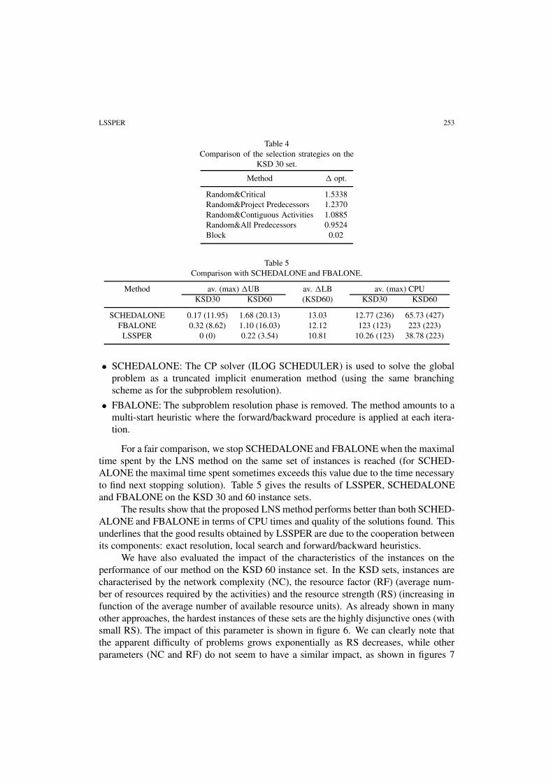
Next, we compare the different selection strategies for the subproblem construc-tion. Table 4 reports the average deviation above the optimal makespan on the KSD30 set obtained by each strategy using ILOG SCHEDULER as subproblem resolutionmethod. The results clearly show that the block strategy outperforms the other ones.

Since our method has several interacting components, we have to compare ourresults with the ones obtained by each component used separately as a resolution method.Namely, we compare our method with the 2 following heuristics:

LSSPER 253

Table 4Comparison of the selection strategies on the

KSD 30 set.

Method � opt.

Random&Critical 1.5338Random&Project Predecessors 1.2370Random&Contiguous Activities 1.0885Random&All Predecessors 0.9524Block 0.02

Table 5Comparison with SCHEDALONE and FBALONE.

Method av. (max) �UB av. �LB av. (max) CPUKSD30 KSD60 (KSD60) KSD30 KSD60

SCHEDALONE 0.17 (11.95) 1.68 (20.13) 13.03 12.77 (236) 65.73 (427)FBALONE 0.32 (8.62) 1.10 (16.03) 12.12 123 (123) 223 (223)

LSSPER 0 (0) 0.22 (3.54) 10.81 10.26 (123) 38.78 (223)

• SCHEDALONE: The CP solver (ILOG SCHEDULER) is used to solve the globalproblem as a truncated implicit enumeration method (using the same branchingscheme as for the subproblem resolution).

• FBALONE: The subproblem resolution phase is removed. The method amounts to amulti-start heuristic where the forward/backward procedure is applied at each itera-tion.

For a fair comparison, we stop SCHEDALONE and FBALONE when the maximaltime spent by the LNS method on the same set of instances is reached (for SCHED-ALONE the maximal time spent sometimes exceeds this value due to the time necessaryto find next stopping solution). Table 5 gives the results of LSSPER, SCHEDALONEand FBALONE on the KSD 30 and 60 instance sets.

The results show that the proposed LNS method performs better than both SCHED-ALONE and FBALONE in terms of CPU times and quality of the solutions found. Thisunderlines that the good results obtained by LSSPER are due to the cooperation betweenits components: exact resolution, local search and forward/backward heuristics.

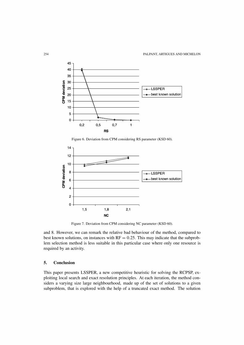
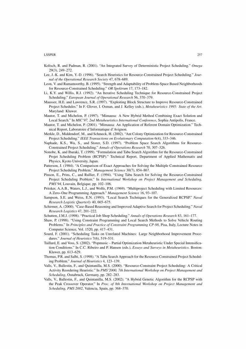
We have also evaluated the impact of the characteristics of the instances on theperformance of our method on the KSD 60 instance set. In the KSD sets, instances arecharacterised by the network complexity (NC), the resource factor (RF) (average num-ber of resources required by the activities) and the resource strength (RS) (increasing infunction of the average number of available resource units). As already shown in manyother approaches, the hardest instances of these sets are the highly disjunctive ones (withsmall RS). The impact of this parameter is shown in figure 6. We can clearly note thatthe apparent difficulty of problems grows exponentially as RS decreases, while otherparameters (NC and RF) do not seem to have a similar impact, as shown in figures 7


Figure 6. Deviation from CPM considering RS parameter (KSD 60).

Figure 7. Deviation from CPM considering NC parameter (KSD 60).

and 8. However, we can remark the relative bad behaviour of the method, compared tobest known solutions, on instances with RF = 0.25. This may indicate that the subprob-lem selection method is less suitable in this particular case where only one resource isrequired by an activity.

5. Conclusion

This paper presents LSSPER, a new competitive heuristic for solving the RCPSP, ex-ploiting local search and exact resolution principles. At each iteration, the method con-siders a varying size large neighbourhood, made up of the set of solutions to a givensubproblem, that is explored with the help of a truncated exact method. The solution

LSSPER 255

Figure 8. Deviation from CPM considering RF parameter (KSD 60).

provided by this partial optimisation is then re-injected into the current solution whichis also post-optimised. The subproblem non-uniform generation procedure, combinedwith periodic re-start of the search, enables to introduce a diversification aspect in theexploration of the search space and to hopefully avoid local optimum.

LSSPER takes place in a more general context where each constituting modulecan be specified independently. Thus, this general method proposes an adaptable globalframework for solving various combinatorial optimisation problems.

Notes

1. The selected activity i has the smallest latest finish time LFi . LFj ’s are computed by backward recursionin the project network (ignoring resources) after assigning LFn+1 to a given upper bound.

2. Results available at http://www.bwl.uni-kiel.de/Prod/psplib/library.html

References

Adams, J., Balas, E., and Zawack, D. (1988). “The Shifting Bottleneck Procedure for Job Shop Scheduling.”Management Science 34, 391–401.

Ahuja, R.K., Ergun, O., Orlin, J.B., and Punnen, A.P. (2002). “A Survey of Very Large-Scale NeighborhoodSearch Techniques.” Discrete Applied Mathematics 123(1–3), 75–102.

Alvarez-Valdés, R. and Tamarit, J.M. (1989). “Heuristic Algorithms for Resource-Constrained ProjectScheduling: A Review and an Empirical Analysis.” In R. Słowinski and J. Weglarz (eds.), Advancesin Projet Scheduling. Amsterdam: Elsevier, pp. 113–134.

Applegate, D. and Cook, B. (1991). “A Computational Study of the Job Shop Scheduling Problem.” ORSAJournal of Computing 3(2), 149–156.

Artigues, C., Michelon, P., and Reusser, S. (2003). “Insertion Techniques for Static and Dynamic Resource-Constrained Project Scheduling.” European Journal of Operational Research 149(2), 249–267.


Baar, T., Brucker, P., and Knust, S. (1998). “Tabu-Search Algorithms and Lower Bounds for the Resource-Constrained Project Scheduling Problem.” In S. Voss, S. Martello, I. Osman, and C. Roucairol (eds.),Metaheuristics: Advances and Trends in Local Search Paradigms for Optimization. Kluwer, pp. 1–18.

Balas, E., Lancia, G., Serafini, P., and Vazacopoulos, A. (1998). “Job Shop Scheduling with Deadlines.”Journal of Combinatorial Optimization 1(4), 329–353.

Baptiste, P. and Le Pape, C. (2000). “Constraint Propagation and Decomposition Techniques for HighlyDisjunctive and Highly Cumulative Project Scheduling Problems.” Constraints 5, 119–139.

Baptiste, P., Le Pape, C., and Nuijten, W. (1995). “Constraint-Based Optimization and Approximation forJob-Shop Scheduling.” In AAAI-SIGMAN Workshop on Intelligent Manufacturing Systems, Montreal.

Bell, C.E. and Han, J. (1991). “A New Heuristic Solution Method in Resource-Constrained Project Schedul-ing.” Naval Research Logistics 38, 315–331.

Bent, R. and Van Hentenryck, P. (2001). “A Two-Stage Hybrid Local Search for the Vehicle Routing Prob-lem with Time Windows.” Technical Report CS-01-06, Brown University.

Bouleimen, K. and Lecocq, H. (2003). “A New Efficient Simulated Annealing Algorithm for the Resource-Constrained Project Scheduling Problem.” European Journal of Operational Research 149(2), 249–267.

Brucker, P., Drexl, A., Möring, R., Neumann, K., and Pesch, E. (1999). “Resource-Constrained ProjectScheduling: Notation, Classification, Models, and Methods.” European Journal of Operational Re-search 112, 3–41.

Caseau, Y. and Laburthe, F. (1999). “Effective Forget-and-Extend Heuristics for Scheduling Problems.”In CP-AI-OR’99, Workshop on Integration of AI and OR Techniques in Constraint Programming forCombinatorial Optimization Problems, Ferrara, Italy.

Cho, J.-H. and Kim, Y.-D. (1997). “A Simulated Annealing Algorithm for Resource Constrained ProjectScheduling Problems.” Journal of the Operational Research Society 48, 735–744.

Congram, R., Potts, C., and Van de Velde, S. (2002). “An Iterated Dynasearch Algorithm for the Single-Machine Total Weighted Tardiness Scheduling Problem.” INFORMS Journal on Computing 14(1), 52–67.

Frangioni, A., Necciari, E., and Scutellà, M.G. (2004). “A Multi-Exchange Neighborhood for MinimumMakespan Machine Scheduling Problems.” Journal of Combinatorial Optimization 8(2), 195–220.

Gendreau, M., Pesant, G., and Rousseau L.-M. (2002). “Using Constraint-Based Operators with VariableNeighborhood Search to Solve the Vehicle Routing Problem with Time Windows.” Journal of Heuristics8(1), 43–58.

Glover, F. and Laguna, M. (1997). Tabu Search. Kluwer Academic.Hartmann, S. (1998). “A Competitive Genetic Algorithm for Resource-Constrained Project Scheduling.”

Naval Research Logistics 45, 733–750.Hartmann, S. (1998). “A Self-Adapting Genetic Algorithm for Project Scheduling Under Resource Con-

straints.” Naval Research Logistics 49, 433–448.Hartmann, S. and Kolisch, R. (2000). “Experimental Evaluation of State-of-the-Art Heuristics for the

Resource-Constrained Project Scheduling Problem.” European Journal of Operational Research 127(2),297–316.

Klein, R. and Scholl, A. (1999). “Computing Lower Bound by Destructive Improvement: An Application toResource-Constrained Project Scheduling.” European Journal of Operational Research 112, 322–346.

Kohlmorgen, U., Schmeck, H., and Haase, F. (1999). “Experiences with Fine-Grained Parallel GeneticAlgorithms.” Annals of Operations Research 90, 203–219.

Kolisch, R. (1996). “Serial and Parallel Resource-Constrained Project Scheduling Methods Revisited: The-ory and Computation.” European Journal of Operational Research 90, 320–333.

Kolisch, R., Sprecher, A., and Drexl, A. (1998). “Benchmark Instances for Project Scheduling Problems.”In J. Weglarz (ed.), Handbook on Recent Advances in Project Scheduling. Kluwer, pp. 197–212.

Kolisch, R. and Hartmann, S. (1999). “Heuristic Algorithms for the Resource-Constrained Project Schedul-ing Problem: Classification and Computational Analysis.” In J. Weglarz (ed.), Project Scheduling: Re-cent Models, Algorithms and Applications. Kluwer, pp. 147–178.

LSSPER 257

Kolisch, R. and Padman, R. (2001). “An Integrated Survey of Deterministic Project Scheduling.” Omega29(3), 249–272.

Lee, J.-K. and Kim, Y.-D. (1996). “Search Heuristics for Resource-Constrained Project Scheduling.” Jour-nal of the Operational Research Society 47, 678–689.

Leon, V. and Ramamoorthy, B. (1995). “Strength and Adaptability of Problem-Space Based Neighborhoodsfor Resource-Constrained Scheduling.” OR Spektrum 17, 173–182.

Li, K.Y. and Willis, R.J. (1992). “An Iterative Scheduling Technique for Resource-Constrained ProjectScheduling.” European Journal of Operational Research 56, 370–379.

Mausser, H.E. and Lawrence, S.R. (1997). “Exploiting Block Structure to Improve Resource-ConstrainedProject Schedules.” In F. Glover, I. Osman, and J. Kelley (eds.), Metaheuristics 1995: State of the Art.Maryland: Kluwer.

Mautor, T. and Michelon, P. (1997). “Mimausa: A New Hybrid Method Combining Exact Solution andLocal Search.” In MIC’97, 2nd Metaheuristics International Conference, Sophia Antipolis, France.

Mautor, T. and Michelon, P. (2001). “Mimausa: An Application of Referent Domain Optimization.” Tech-nical Report, Laboratoire d’Informatique d’Avignon.

Merkle, D., Middendorf, M., and Schmeck, H. (2002). “Ant Colony Optimization for Resource-ConstrainedProject Scheduling.” IEEE Transactions on Evolutionary Computation 6(4), 333–346.

Naphade, K.S., Wu, S., and Storer, S.D. (1997). “Problem Space Search Algorithms for Resource-Constrained Project Scheduling.” Annals of Operations Research 70, 307–326.

Nonobe, K. and Ibaraki, T. (1999). “Formulation and Tabu Search Algorithm for the Resource-ConstrainedProjet Scheduling Problem (RCPSP).” Technical Report, Department of Applied Mathematis andPhysics, Kyoto University, Japan.

Patterson, J. (1984). “A Comparison of Exact Approaches for Solving the Multiple Constrained ResourceProject Scheduling Problem.” Management Science 30(7), 854–867.

Pinson, E., Prins, C., and Rullier, F. (1994). “Using Tabu Search for Solving the Resource-ConstrainedProject Scheduling Problem.” In International Workshop on Project Management and Scheduling,PMS’94, Louvain, Belgique, pp. 102–106.

Pritsker, A.A.B., Waters, L.J., and Wolfe, P.M. (1969). “Multiproject Scheduling with Limited Resources:A Zero–One Programming Approach.” Management Science 16, 93–107.

Sampson, S.E. and Weiss, E.N. (1993). “Local Search Techniques for the Generalized RCPSP.” NavalResearch Logistic Quarterly 40, 665–675.

Schirmer, A. (2000). “Case-Based Reasoning and Improved Adaptive Search for Project Scheduling.” NavalResearch Logistics 47, 201–222.

Schutten, J.M.J. (1998). “Practical Job Shop Scheduling.” Annals of Operations Research 83, 161–177.Shaw, P. (1998). “Using Constraint Programming and Local Search Methods to Solve Vehicle Routing

Problems.” In Principles and Practice of Constraint Programming CP-98, Pisa, Italy, Lecture Notes inComputer Science, Vol. 1520, pp. 417–431.

Sourd, F. (2001). “Scheduling Tasks on Unrelated Machines: Large Neighborhood Improvement Proce-dures.” Journal of Heuristics 7(6), 519–531.

Taillard, E. and Voss, S. (2002). “Popmusic – Partial Optimization Metaheuristic Under Special Intensifica-tion Conditions.” In C.C. Ribeiro and P. Hansen (eds.), Essays and Surveys in Metaheuristics. Boston:Kluwer, pp. 613–629.

Thomas, P.R. and Salhi, S. (1998). “A Tabu Search Approach for the Resource Constrained Project Schedul-ing Problem.” Journal of Heuristics 4, 123–139.

Valls, V., Ballestin, F., and Quintanilla, M.S. (2000). “Resource-Constraint Project Scheduling: A CriticalActivity Reordering Heuristic.” In PMS’2000, 7th International Workshop on Project Management andScheduling, Osnabruck, Germany, pp. 282–283.

Valls, V., Ballestin, F., and Quintanilla, M.S. (2002). “A Hybrid Genetic Algorithm for the RCPSP withthe Peak Crossover Operator.” In Proc. of 8th International Workshop on Project Management andScheduling, PMS 2002, Valencia, Spain, pp. 368–370.

lssper: solving the resource-constrained project scheduling problem with large neighbourhood search

Documents