ls(graph): a constraint-based local search for constraint optimization on trees and paths
TRANSCRIPT

Constraints (2012) 17:357–408DOI 10.1007/s10601-012-9124-0
LS(Graph): a constraint-based local searchfor constraint optimization on trees and paths
Quang Dung Pham · Yves Deville ·Pascal Van Hentenryck
Published online: 12 July 2012© Springer Science+Business Media, LLC 2012
Abstract Constrained optimum tree (COT) and constrained optimum path (COP)problems arise in many real-life applications and are ubiquitous in communicationnetworks. They have been traditionally approached by dedicated algorithms, whichare often hard to extend with side constraints and to apply widely. This paperproposes a constraint-based local search framework for COT/COP applications,bringing the compositionality, reuse, and extensibility at the core of constraint-basedlocal search and constraint programming systems. The modeling contribution is theability to express compositional models for various COT/COP applications at a highlevel of abstraction, while cleanly separating the model and the search procedure.The main technical contribution is a connected neighborhood based on rootedspanning trees to find high-quality solutions to COP problems. This framework isapplied to some COT/COP problems, e.g., the quorumcast routing problem, theedge-disjoint paths problem, and the routing and wavelength assignment with delayside constraints problem. Computational results show the potential importance ofthe approach.
Keywords Combinatorial optimization · Constraint-based local search · Graphs ·Constrained optimum trees · Constrained optimum paths · Quorumcast routing ·Edge-disjoint paths · Routing and wavelength assignment with delay constraints
Q. D. Pham (B)School of Information and Communication Technology,Hanoi University of Science and Technology, Hanoi, Vietname-mail: [email protected]
Y. DevilleUniversité catholique de Louvain, 1348 Louvain-la-Neuve, Belgiume-mail: [email protected]
P. Van HentenryckOptimization Research Group, NICTA, Victoria Research Laboratory,Electrical and Electronic Engineering, The University of Melbourne,Melbourne, VIC 3010, Australiae-mail: [email protected]

358 Constraints (2012) 17:357–408
1 Introduction
Constrained optimum tree (COT) and constrained optimum path (COP) problemsappear in various real-life applications such as telecommunication and transportationnetworks. These problems consist of finding one or more trees (or paths) on a givengraph satisfying some given constraints while minimizing or maximizing an objectivefunction. Some COT problems have been considered and solved in the literature,e.g., Degree Constrained Minimum Spanning Tree (DCMST) [7, 45], BoundedDiameter Minimum Spanning Tree (BDMST) [35], Capacitated Minimum SpanningTree problem (CMST) [3, 56], Minimum Diameter Spanning Tree (MDST) [50],Edge-Weighted k-Cardinality Tree (KCT), [20, 25], Steiner Minimal Tree (SMT)[28, 66], Optimum Communication Spanning Tree problems (OCST) [32], etc. Wealso see many COP problems which have been studied and solved in the liter-ature. For instance, in telecommunication networks, routing problems supportingmultiple services involve the computation of paths minimizing transmission costswhile satisfying bandwidth and delay constraints [15, 27, 30]. Similarly, the problemof establishing routes for connection requests between network nodes is one ofthe basic operations in communication networks and it is typically required thatno two routes interfere with each other due to quality-of-service and survivabilityrequirements. This problem can be modeled as an edge-disjoint paths problem[18]. Most of these COT/COP problems are NP-hard. They are often approachedby dedicated algorithms including exact methods, such as the Lagrangian-basedheuristic [7], the ILP-based algorithm using directed cuts [25], the Lagrangian-basedbranch and bound in [15], and the vertex labeling algorithm from [30]; there are alsometa-heuristic algorithms such as a hybrid evolutionary algorithm [19], ant colonyoptimization [21], and local search [20]. These techniques exploit the structure of theconstraints and the objective functions but are often difficult to extend or reuse.
This paper1 proposes a constraint-based local search (CBLS) [62] framework forCOT/COP applications to support the compositionality, reuse, and extensibility atthe core of CBLS and CP systems. It follows the trend of defining domain-specificCBLS frameworks, capturing modeling abstractions and neighborhoods for classes ofapplications exhibiting significant structures. As is traditional for CBLS, the resultingLS(Graph) framework allows the model to be compositional and easy to extend,and provides a clean separation of concerns between the model and the searchprocedure. Moreover, the framework captures structural moves that are fundamentalin obtaining high-quality solutions for COT/COP applications. The key technicalcontribution underlying this COP framework is a novel connected neighborhood forCOP problems based on rooted spanning trees. More precisely, this COP frameworkincrementally maintains, for each desired elementary path, a rooted spanning treethat specifies the current path and provides an efficient data structure to obtain itsneighboring paths and their evaluations.
The availability of high-level abstractions (the “what”) and the underlyingconnected neighborhood for elementary paths (the “how”) make the LS(Graph)framework particularly appealing for modeling and solving complex COPapplications.
1This paper is an extended version of [54] and is based on the PhD thesis [53].

Constraints (2012) 17:357–408 359
The LS(Graph) framework, implemented in COMET, was evaluated experimen-tally on two classes of applications: COT with the quorumcast routing (QR)problem and COP with the edge-disjoint path (EDP) problems and the routingand wavelength assignment problem with side constraints (RWA-D). In [37], wepresent another application in the domain of traffic engineering in switched ethernetnetworks. The experimental results show the potential of the approach.
1.1 Case studies
We first describe three problems that will be modeled and solved by the LS(Graph)framework.
1.1.1 The quorumcast routing (QR) problem
The quorumcast routing (QR) problem arises in distributed applications [24, 29, 48,63]. Given a weighted undirected graph G = (V, E), to each edge e ∈ E there isassociated a cost w(e). Given a source node r ∈ V, an integral value q, and a set S ⊆ Vof multicast nodes, the quorumcast routing problem consists in finding a minimumcost tree T = (V ′, E′) of G spanning r and q nodes of S. T = (V ′, E′) is a graphsatisfying the following properties:
1. V ′ ⊆ V ∧ E′ ⊆ E.2. T is connected.3. ∃Q ⊆ S such that �Q = q ∧ Q ∪ {r} ⊆ V ′.4. The cost of
T =∑
e∈E′w(e)
is minimal over all subgraphs of G with properties 1–3.
An exact algorithm [48] has also been proposed for solving the QR problem butexperiments were performed on small graphs (e.g., graph with 30 nodes). Threeheuristics have been proposed in [24] including Minimal Cost Path Heuristic (MPH),Improved Minimum Path Heuristic (IMP), and Modified Average Distance Heuris-tic (MAD). Experimental results in that paper show that, among these heuristics, theIMP heuristic produces the best solutions. In [29], a multispace search heuristic hasbeen proposed for solving this problem which gives better results than the IMP andthe MAD heuristics on 12-node networks and 100-node networks.
In [63], the authors considered the QR problem with additional constraintsimposed on the total cumulative delay along the path from s to any destination nodeof Q, and proposed a distributed heuristic algorithm for solving it. Experiments wereconducted on graphs of up to 200 nodes.
In Section 6.1, we propose a simple model in LS(Graph) for this problem usinga tabu search. This example illustrates the expressive power of LS(Graph) where asimple but efficient model can be designed in a few lines. Experimental results showthat our LS(Graph) model gives better results than the standard IMP heuristic.

360 Constraints (2012) 17:357–408
1.1.2 The edge-disjoint paths (EDP) problem
We are given an undirected graph G = (V, E) and a set T = {〈si, ti〉 | i = 1, 2,..., �T; si = ti ∈ V} representing a list of commodities. A subset T ′ ⊆ T, T ′ ={〈si1 , ti1〉, ..., 〈sik , tik〉} is called edp-feasible if there exist mutually edge-disjoint pathsfrom si j to ti j on G, ∀ j = 1, 2, .., k. The EDP problem consists in finding a edp-feasiblesubset of T with maximal cardinality. In other words,
max �T ′ (1)
s.t. T ′ ⊆ T (2)
T ′ is edp-feasible (3)
This problem appears in many applications such as real-time communication,VLSI-design, routing, and admission control in modern networks [8, 23]. The existingtechniques for solving this problem include approximation algorithms [13, 22, 42, 43],greedy approaches [42, 44], and an ant colony optimization (ACO) metaheuristic[18]. It has been shown in [18] that ACO is the start-of-the-art algorithm for thisproblem. In that paper, the ACO algorithm were compared with a simple greedyalgorithm in [42](the multi-start version).
In Section 6.2, we propose two heuristic algorithms applying LS(Graph). Weexperimentally show competitive results compared with the ACO algorithm in [18].This example illustrates how LS(Graph) can be used to implement more complexheuristics.
1.1.3 The routing and wavelength assignment problem with a delay side constraint(RWA-D)
Wavelength division multiplexing (WDM) optical networks [49] provide high band-width communications. The routing and wavelength assignment (RWA) problemis an essential problem on WDM optical networks. The RWA problem can bedescribed as follows. Given a set of requests for all-optical connections, the RWAproblem consists of finding routes from the source nodes to their respective desti-nation nodes and assigning wavelengths to these routes. A condition that must besatisfied is that two routes sharing common edges must be assigned different wave-lengths. Normally, the number of available wavelengths is limited and the numberof requests is high. Two variants of this problem have been studied extensively inthe literature: the minRWA problem aims at minimizing the number of wavelengthused for satisfying all requests, and the maxRWA aims at maximizing the number ofrequests with a given number of wavelengths. Both variants are NP-Hard [26].
In the literature, there have been different techniques proposed for solving theseproblems, e.g.: exact methods based on the ILP formulation [23, 40, 46, 47, 52, 55, 61,65]; heuristic algorithms [11, 12, 31, 67]; and metaheuristics, including tabu search [39,51] and Genetic [4, 10, 38]. These techniques have been tried on realistic networksof small size (networks up to 27 nodes and 70 edges) but involving a large numberof connection requests. RWA with additional constraints has also been considered,e.g., in [5, 64].
In order to show the interest of the modeling framework, we consider theminRWA problem with a side constraint (e.g., a delay constraint) specifying that thecost of each route must be less than or equal to a given value. The point here is not to

Constraints (2012) 17:357–408 361
study a model competitive in comparison with state-of-the-art techniques for classicalRWA problems. Rather, we show the flexibility of this modeling framework, onewhich enables a combination of VarGraph of LS(Graph) with var{int} of COMET.
The formal definition of the problem (called RWA-D) is the following. Givenan undirected weighted graph G = (V, E), each edge e of G has cost c(e) (e.g.,the delay in traversing e). We suppose given a set of connection requests R ={〈s1, t1〉, 〈s2, t2〉, ..., 〈sk, tk〉} and a value D. The RWA-D problem consists of findingroutes pi from si to ti and their wavelengths for all i = 1, 2, ..., k such that:
1. the wavelengths of pi and pj are different if they have common edges, ∀i = j ∈{1, 2, ..., k} (wavelength constraint),
2.∑
e∈pic(e) ≤ D,∀i = 1, 2, ..., k (delay constraint)
3. the number of different wavelengths is minimized (objective function).
In Section 6.3, a local search algorithm and its implementation in LS(Graph) will beproposed for solving the RWA-D problem.
1.2 Contribution
The contributions of this paper are the following:
1. We design and implement a constraint-based local search (CBLS) [62] frame-work, called LS(Graph), for COT/COP applications. It supports the compo-sitionality, reuse, and extensibility at the core of CBLS and CP systems. Theproposed framework can be used as either a black box or a glass box. Theblack box is exploited in the sense that users only need to state the model ina declarative way, with variables, constraints, and an objective function to beoptimized. Built-in search components (e.g., tabu search) are then performedautomatically. The glass box allows users to extend the framework by designingand implementing their own components (e.g., invariants, constraints, objectivefunctions, and search heuristics) and integrating them with the system.
2. The LS(Graph) combines graph variables (i.e., VarTree, VarPath for mod-eling trees and paths in a high-level way) with standard var{int} of COMET,which enables the modeling of various COT/COP applications on graphs forwhich both the topology and scalar values must be determined.
3. A key technical contribution of the paper is a novel connected neighborhoodfor COP problems based on rooted spanning trees. More precisely, the COPframework incrementally maintains, for each desired elementary path, a rootedspanning tree that specifies the current path and provides an efficient datastructure to obtain its neighboring paths and their evaluations.
4. We propose incremental algorithms for implementing some fundamental ab-stractions of the framework. We show that the incrementality does not improvethe theoretical complexity but is efficient in practice.
5. We apply the constructed framework to a COT problems: the quorumcastrouting problem and two COP problems: the edge-disjoint paths problem andthe routing and wavelength assignment problem with delay side constraints onoptical networks. Experimental results show the potential significance of ourapproach from both the programming and the computation stand points. For

362 Constraints (2012) 17:357–408
the first two problems, we show competitive results in comparison with existingtechniques and for the third problem, we show how to solve complex problemsflexibly and easily.
The LS(Graph) framework is open source. The COMET code of LS(Graph)and applications as well as instances experimented in this paper are available athttp://becool.info.ucl.ac.be/lsgraph.
1.3 Outline
The rest of this paper is organized as follows. Section 2 gives the basic definitions andnotations. Section 3 specifies neighborhoods for COT applications and proposes ournovel neighborhoods for COP applications. Section 4 gives an overview of data struc-tures and algorithms for implementing two fundamental and non-trivial abstractionsof the framework. The implementation of the framework in COMET programminglanguage will be introduced in Section 5. Sections 6 presents the application ofthe framework to the resolution of the QR, EDP and RWA-D problems. Finally,Section 7 concludes the paper and gives some future work.
2 Definitions and notations
Graphs Given an undirected graph g, we denote the set of nodes and the set ofedges of g by V(g), E(g) respectively. The degree of a node v (denoted degg(v)) isthe number of incident edges to this edge: degg(v) = �{u | (v, u) ∈ V(g)}.
A graph sg is called subgraph of a graph g if V(sg) ⊆ V(g) and E(sg) ⊆ E(g) andwe denote sg ⊆ g.
A path on g is a sequence of nodes 〈v1, v2, ..., vk〉 (k > 1) in which vi ∈ V(g)
and (vi, vi+1) ∈ E(g),∀i = 1, . . . , k − 1. The nodes v1 and vk are the origin and thedestination of the path. A path is called simple if there is no repeated edge andelementary if there is no repeated node. A cycle is a path in which the origin andthe destination are the same. This paper only considers elementary paths and hencewe use “path” and “elementary path” interchangeably if there is no ambiguity. Agraph is connected if and only if there exists a path from u to v for all u, v ∈ V(g).
Given two paths px = 〈x1, x2, ..., xk〉 and py = 〈y1, y2, ..., yq〉, we denote px + pythe concatenation of these two paths: px + py = 〈x1, x2, ..., xk, y1, y2, ...yq〉 if xk = y1
and px + py = 〈x1, x2, ..., xk = y1, y2, ..., yq〉 if xk = y1.Given paths p, p1, p2, and q,
– V(p) is the set of nodes of p– p1 ∪ p2 (p1 ∩ p2) is the set V(p1) ∪ V(p2) (V(p1) ∩ V(p2)).– x ∈ P is the predicate x ∈ V(p).– s(p), t(p) are, respectively, the starting and terminating nodes of p.– p(u, v) is the subpath of p starting from u and terminating at v (u, v ∈ p and u is
not located after v on p).– spp(x), tpp(x) is the subpath of p from s(p) to x and from x to t(p).– repl(p, q) = spp(s(q)) + q + tpp(t(q)) with s(q), t(q) ∈ p. Intuitively, repl(p, q) is
the path generated by replacing the subpath of p from s(q) to t(q) by q.

Constraints (2012) 17:357–408 363
Fig. 1 Illustrating Property 1
13
z 2
3
45
y
x
8
v11
12
14
Trees A tree is an undirected connected graph containing no cycles. A spanning treetr of an undirected connected graph g is a tree spanning all the nodes of g: V(tr) =V(g) and E(tr) ⊆ E(g). A tree tr is called a rooted tree at r if the node r has beendesignated the root. Each edge of tr is implicitly oriented towards the root. If theedge (u, v) is oriented from u to v, we call v the father of u in tr, which is denoted byfatr(u). Given a rooted tree tr and a node s ∈ V(tr),
– root(tr) denotes the root of tr,– pathtr(v) denotes the path from v to root(tr) on tr. For each node u of pathtr(v),
we say that u dominates v in tr (alternatively, u is a dominator of v, v is adescendant of u) which we denote by u Domtr v. If u does not dominates v ontr, we write u Domtr v.
– pathtr(u, v) denotes the path from u to v in tr (u, v ∈ V(tr)).– ncatr(u, v) denotes the nearest common ancestor of two nodes u and v. In other
words, ncatr(u, v) is the common dominator of u and v such that there is no othercommon dominator of u and v that is a descendant of ncatr(u, v).
– Given a node v ∈ V(tr), we denote by Ttr(v) the subtree of tr rooted at v. Ifv = root(tr), we denote by Ttr(v) the subtree of tr generated by removing Ttr(v)
and the edge (v, fatr(v)) from tr: V(Ttr(v)) = V(tr) \ V(Ttr(v)) and E(Ttr(v)) =E(tr) \ (E(Ttr(v)) ∪ {(v, fatr(v))}).
Property 1 Suppose given a rooted tree tr.
1. Suppose given a node x ∈ V(tr). We have x Domtr y,∀y ∈ V(Ttr(x)). In otherwords, a vertex x of a rooted tree tr dominates all vertices of the subtree of trrooted at x.

364 Constraints (2012) 17:357–408
2. Suppose given two nodes x, y ∈ V(tr) such that x = fatr(y) and two nodes z, v
such that z ∈ V(Ttr(y)), v ∈ V(Ttr(y)). We have ncatr(v, z) = ncatr(v, x). Thisproperty is illustrated in Fig. 1: ncatr(v, z) = ncatr(v, x) = 12.
3 Neighborhoods
This section defines neighborhoods for COT and COP problems. The neighborhoodfor COT applications is based on traditional modification actions on dynamic trees(i.e., trees which can be modified): add, remove, and replace over edges. Our maintechnical contribution for COP applications is to propose a neighborhood structurebased on spanning trees. We first present neighborhoods for COT applications.
3.1 COT neighborhood
A neighborhood of a tree is a set of trees generated by performing modificationactions on the given tree. Given an undirected graph g and a dynamic tree tr of g (trcan be modified such that tr ⊆ g), we specify a set of basic modifications conservingthe tree property. We consider in this framework the following basic modifications.
1. add edge action An edge e = (u, v) ∈ E(g) \ E(tr) can be added to tr if tr isempty, or if there is exactly one node u or v in the tree tr: u ∈ V(tr) XOR v ∈ V(tr).This edge is called an insertable edge. The insertion of this edge implicitly addsits endpoints to tr if they do not exist in tr. The set of insertable edges of tr isdenoted by Inst(tr) and this insertion action is denoted by addEdge(tr, e). Wealso use addEdge(tr, e) to denote the resulting tree. The first basic neighborhoodis the following:
NT1(tr) = {addEdge(tr, e) | e ∈ Inst(tr)}2. remove edge action An edge e = (u, v) ∈ E(tr) can be removed from tr if one
node u or v is a leaf of tr: degtr(u) = 1 ∨ degtr(v) = 1. This edge is called aremovable edge. The removal of this edge thus also removes its endpointsif they are the leaves of tr. The set of removable edges of tr is denoted byRemv(tr) and this removal action is denoted by removeEdge(tr, e). We also useremoveEdge(tr, e) to denote the resulting tree. The second basic neighborhood isdefined as follows:
NT2(tr) = {removeEdge(tr, e) | e ∈ Remv(tr)}3. replace cycle edge action [2] An edge e′ of tr can be replaced by another edge
e = (u, v) ∈ E(g) \ E(tr) with u, v ∈ V(tr) conserving the tree property in thefollowing case: the insertion of e creates a fundamental cycle containing e′ andthe removal of e′ removes the cycle and restores the tree property. The edge e iscalled a replacing edge, and e′ is called a replaceable edge of e. The set of nodes oftr is unchanged by this replacement. We denote by Repl(tr) the set of replacingedges of tr and Repl(tr, e) the set of replaceable edges of the replacing edge e. Weuse replaceEdge(tr, e′, e) to denote both the replacement action and the resultingtree. The third basic neighborhood is defined as follows:
NT3(tr) = {replaceEdge(tr, e′, e) | e ∈ Repl(tr) ∧ e′ ∈ Repl(tr, e)}

Constraints (2012) 17:357–408 365
In practice, we can combine the above basic moves to perform more complexmoves. For instance, we take addEdge(tr, e1) and removeEdge(tr, e2) at hand wheree1 ∈ Remov(tr) and e2 ∈ Inst(tr) and e1 and e2 do not have common endpoint that isthe leaf tr.2 The set of such pairs of 〈e1, e2〉 is denoted by RemvInst(tr). This kind ofneighborhood has been considered in the tabu search algorithm of [20]. The formaldefinition of this neighborhood is
NT1+2(tr) = {addEdge(removeEdge(tr, e2), e1) | 〈e1, e2〉 ∈ RemvInst(tr)}In the following section, we introduce a novel neighborhood for COP applications.
3.2 COP neighborhood
We consider in this paper only elementary paths, i.e., paths having no repeatedvertices. These are those which appear in most COP applications. Our constructedframework also supports the modeling of paths where vertices or edges can berepeated, but this will not be presented here (see more details in [53]).
For COP problems, a neighborhood of a path defines a set of paths that can bereached from the current path. The most general neighborhood of a path p on a givengraph g is defined as the set of paths generated by replacing a subpath of the currentpath by another path on the given graph conserving the path property: N (p) ={repl(p, q) | q ∈ R(p)} in which R(p) is the set of paths q satisfying followingsconditions:
(1) q ∈ g(2) s(q), t(q) ∈ p(3) spp(s(q)) ∩ q = {s(q)}(4) tpp(t(q)) ∩ q = {t(q)}
Conditions (3) and (4) ensure the path property of all elements of N (p) (norepeated vertices are allowed in a path except starting and terminating vertices).3
Unfortunately, such a neighborhood is too large and does not allow being exploredin a generic way. To overcome this difficulty, in this section, we propose a restrictedneighborhood based on rooted spanning trees. This notion can be widely applied andallows users to perform efficient neighborhood explorations.
Related work As far as we know, there exist only a few local search approachesfor COP applications on general graphs. Moreover, these local search algorithmsdo not explicitly describe neighborhood structures. Rather, the authors talk aboutthe moves, which are very specific and sophisticated. Such moves do not enable thecompositionality, modularity, and reuse of the local search programs.
On complete graphs, some local search algorithms have been applied for solvingthe traveling salesman problem [41] or the vehicle routing problem [9, 34]. In theseapproaches, a path is explicitly represented by a sequence of vertices and the neigh-borhood consists of paths generated by changing some vertices of this sequence (e.g.,by removing, inserting, exchanging, or changing the position of some vertices). These
2This condition ensures the preservation of the tree property under the modification action.3By some authors, walks with no repeated vertices are referred to as elementary paths.

366 Constraints (2012) 17:357–408
neighborhood structures cannot be applied to general graphs because a sequence ofvertices can not be guaranteed to always form a path on the given graph.
To obtain a reasonable efficiency, a local search algorithm must maintain incre-mental data structures that allow a fast exploration of this neighborhood and a fastevaluation of the impact of the moves (differentiation). The key novel contributionof our COP framework is to use a rooted spanning tree to represent the currentsolution and its neighborhood. It is based on the observation that, given a spanningtree tr whose root is t, the path from a given node s to t in tr is unique. Moreover, thespanning tree implicitly specifies a set of paths that can be reached from the inducedpath and provides a data structure for evaluating their desirability. The rest of thissection describes the neighborhood in detail. Our COP framework considers bothdirected and undirected graphs, but, to simplify the presentation, only undirectedgraphs are treated.
3.2.1 Rooted spanning trees
Given an undirected graph g and a target node t ∈ V(g), our COP neighborhoodmaintains a spanning tree of g rooted at t. Moreover, since we are interested inelementary paths between a source s and a target t, the data structure also maintainsthe source node s and is called a rooted spanning tree (RST) over (g, s, t). An RSTtr over (g, s, t) specifies a unique path from s to t in g: pathtr(s) = 〈v1, v2, ..., vk〉 inwhich s = v1, t = vk and vi+1 = fatr(vi), ∀i = 1, . . . , k − 1. By maintaining RSTs forCOP problems, our framework avoids an explicit representation of the paths andenables the definition of a connected neighborhood that can be explored efficiently.Indeed, the tree structure directly captures the path structure from a node s to theroot; simple updates to the RST (e.g., an edge replacement) will induce a new pathfrom s to the root. In this framework, we also consider COP applications in whichthe sources and the destinations of the paths are not fixed. Hence, the source s andthe destination (or root) of the RST (g, s, t) can also be changed (but this will not bepresented in this paper, interested readers can refer to the PhD thesis [53]).
Given an RST tr over (g, s, t), we denote by path(tr) the path pathtr(s) which isthe path induced by tr from s to the root t of tr. Given an undirected graph g and apath p on g, we denote by RSTInduce(g,p) the set of RSTs of g, rooted at t(p), whichinduce p.
We define in the following section the neighborhood structure based on edgereplacements. In COP applications, generally, a candidate solution is a set of paths.Each path has its own neighborhood. A neighborhood of a candidate solution is theset of candidate solutions generated by changing some paths of the current candidatesolution with their neighbors. Hence, we present only neighborhoods of one path.
3.2.2 The edge-replacement based neighborhood
We first show in this section how to update an RST tr over (g, s, t) based on edgereplacements to generate a new rooted spanning tree tr′ over (g, s, t) which induces anew path from s to t in g: pathtr′(s) = pathtr(s).
Let tr be an RST over (g, s, t), we consider the third basic neighborhood of tr (seeSection 3.1):
NT3(tr) = {replaceEdge(tr, e′, e) | e ∈ Repl(tr) ∧ e′ ∈ Repl(tr, e)}

Constraints (2012) 17:357–408 367
which is the set of RST of (g, s, t). It is easy to observe that two RSTs tr1 and tr2
over (g, s, t) may induce the same path from s to t. For this reason, we now showhow to compute a subset ERNP1(tr) ⊆ NT3(tr) such that pathtr′(s) = pathtr(s),∀tr′ ∈ERNP1(tr).
We first fix some notations to be used in the following presentation. Given anRST tr over (g, s, t) and a replacing edge e = (u, v), the nearest common ancestorsof s and the two endpoints u, v of e are both located on the path from s to t. Wedenote by lowncatr(e, s) and upncatr(e, s) the nearest common ancestors of s on theone hand and one of the two endpoints of e on the other hand, with the conditionthat upncatr(e, s) dominates lowncatr(e, s). We denote by lowtr(e, s), uptr(e, s) theendpoints of e such that ncatr(s, lowtr(e, s)) = lowncatr(e, s) and ncatr(s, uptr(e, s)) =upncatr(e, s). Figure 2 illustrates these concepts. The left part of the figure depictsthe graph g and the right side depicts an RST tr over (g, s, r). Edge (8,10) is areplacing edge of tr; ncatr(s, 10) = 12 since 12 is the common ancestor of s and 10.ncatr(s, 8) = 7 since 7 is the common ancestor of s and 8. lowncatr((8, 10), s) = 7 andupncatr((8, 10), s) = 12 because 12 Domtr 7; lowtr((8, 10), s) = 8; uptr((8, 10), s) = 10.
We now specify the replacements that induce a new path from s to t.
Proposition 1 Let tr be an RST over (g, s, t), e = (u, v) be a replacing edge of tr, lete′ be a replaceable edge of e, and let tr′ = rep(tr, e′, e). Let su = upncatr(e, s) and sv =lowncatr(e, s). We have that pathtr′(s) = pathtr(s) if and only if
(1) su = sv and(2) e′ ∈ pathtr(sv, su)
A replacing edge e of tr satisfying the condition (1) is called a preferred replacingedge and a replaceable edge e′ of e in tr satisfying condition (2) is called a preferred
s
1 2
3
45
6
7
8
1011
12
t
a. The undirected graph g
s
1 2
3
45
6
7
8 lowtr ((8 , 10) , s )
10 uptr ((8 , 10) , s )11
12upncatr((8 , 10) , s )
lowncatr ((8 , 10) , s )
t
b. A spanning tree tr rooted at t of g
Fig. 2 An example of rooted spanning tree

368 Constraints (2012) 17:357–408
replaceable edge of e. We denote by prefRepl(tr) the set of preferred replacing edgesof tr and by prefRepl(tr, e) the set of preferred replaceable edges of the preferredreplacing edge e on tr. We also denote by rep(tr, e′, e) the action and the resultingRST of replacing a preferred replaceable edge e′ by a preferred replacing edge e onthe RST tr. The edge-replacement based neighborhood (called ER-neighborhood)of an RST tr is defined by
ERNP1(tr) = {tr′ = rep(tr, e′, e) | e ∈ prefRepl(tr), e′ ∈ prefRepl(tr, e)}.The action rep(tr, e′, e) is called an ER-move and is illustrated in Fig. 3. In the currenttree tr (see Fig. 3a), the edge (8,10) is a preferred replacing edge, ncatr(s, 8) = 7,ncatr(s, 10) = 12, lowncatr((8, 10), s) = 7, upncatr((8, 10), s) = 12, lowtr((8, 10), s) = 8and uptr((8, 10), s) = 10. The edges (7,11) and (11,12) are preferred replaceableedges of (8,10) because these edges belong to pathtr(7, 12). The path induced by tr is〈s, 3, 4, 6, 7, 11, 12, t〉. The path induced by tr′ is 〈s, 3, 4, 6, 7, 8, 10, 12, t〉 (see Fig. 3b).
ER-moves ensure that the neighborhood is connected, which is explained in detailin Proposition 2.
Proposition 2 Let tr0 be an RST over (g, s, t) and P be a path from s to t. An RSTinducing P can be reached from tr0 in k ≤ l basic moves, where l is the length of P .
3.2.3 Neighborhood of independent ER-moves
It is possible to consider more complex moves by applying a set of indepen-dent ER-moves. Two ER-moves are independent if the execution of the firstone does not affect the second one and vice versa. The sequence of ER-moves〈rep(tr, e′
1, e1), . . . , rep(tr, e′k, ek)〉, denoted by rep(tr, e′
1, e1, e′2, e2, ..., e′
k, ek), is definedas the application of the sequence of actions 〈rep(tr1, e′
1, e1), rep(tr2, e′2, e2), . . .,
Fig. 3 Illustrating a basicmove
s
1 2
3
45
6
7
8
1011
12
t
a. current tree tr
s
1 2
3
45
6
7
8
1011
12
t
b. tr = rep(tr, (7 , 11) , (8 , 10))

Constraints (2012) 17:357–408 369
rep(trk, e′k, ek)〉, where tr1 = tr and tr j+1 = rep(tr j, e′
j, e j), ∀ j = 1, . . . , k − 1. It is fea-sible if the ER-moves are feasible, i.e., e j ∈ prefRpl(tr j) and e′
j ∈ prefRpl(tr j, e j).
Proposition 3 Consider k ER-moves rep(tr, e′1, e1), . . . , rep(tr, e′
k, ek). If all pos-sible execution sequences of these basic moves are feasible and the edgese′
1, e1, e′2, e2, . . . , e′
k, ek are all dif ferent, then these k ER-moves are independent.
We denote by ERNPk(tr) the set of neighbors of tr obtained by applying kindependent ER-moves. The action of taking a neighbor in ERNPk(tr) is called anER-k-move.
It remains to find some criterion for whether two ER-moves are independent.Given an RST tr over (g, s, t) and two preferred replacing edges e1, e2, we say thate1 dominates e2 in tr, written e1 Domtr e2, if lowncatr(e1, s) dominates upncatr(e2, s).Then, two preferred replacing edges e1 and e2 are independent w.r.t. tr if e1 dominatese2 in tr or e2 dominates e1 in tr.
Proposition 4 Let tr be an RST over (g, s, t), e1 and e2 be two preferred re-placing edges such that e2 Domtr e1, e′
1 ∈ pref Rpl(tr, e1), and e′2 ∈ pref Rpl(tr, e2).
Then rep(tr, e′1, e1) and rep(tr, e′
2, e2) are independent and the path induced byrep(tr,e′
1,e1,e′2,e2) is pathtr(s, v1) + pathtr(u1, v2) + pathtr(u2, t), where the addition sign
denotes path concatenation and v1 = lowtr(e1, s), u1 = uptr(e1, s), v2 = lowtr(e2, s),and u2 = uptr(e2, s).
Figure 4 illustrates a complex move. In tr, the two preferred replacing edgese1 = (1, 5) and e2 = (8, 10) are independent because lowncatr((8, 10), s) = 7, which
s
1 2
3
45
6
7
8
1011
12
t
e2
e1
e2
e1
a. The Current Tree tr (dashed edges are not included)
s
1 2
3
45
6
7
8
1011
12
t
b. tr = rep (tr, (7 , 11) , (8 , 10) , (3 , 4) , (1 , 5))
Fig. 4 Illustrating a Complex Move

370 Constraints (2012) 17:357–408
dominates upncatr((1, 5), s) = 6 in tr. The new path induced by tr′ is 〈s, 3 ,1, 5, 6, 7, 8,10, 12, t〉, which is actually the path pathtr(s, 1) + pathtr(5, 8) + pathtr(10, t).
4 Data structure and algorithms
In this section, we briefly describe the implementation of some fundamental andnon-trivial abstractions and then analyze their complexities.
4.1 VarTree and nearest common ancestors
VarTree(g) is an abstraction representing a dynamic tree over an undirected graphg that can be modified by removing, inserting an edge, or replacing an edge byanother edge. It also allows querying information about the tree. For facilitatingmanipulations on dynamic trees, the trees are implicitly stored as rooted trees.Several well-known data structures have been proposed for representing dynamictrees, for instance, ST-trees [57, 58], topology trees [33], ET-trees [36], top trees[6, 59], and RC-trees [1] (and the references therein). These data structures maintaina forest of dynamic rooted trees, supporting update actions (e.g., link and cut) andsome queries (e.g., minimum (maximum) cost edge, node on a path, nearest commonancestors of two nodes, medians, centers of a tree) in O(log n) time per operationwhere n is the number of vertices of the given graph. These data structures have beenexperimentally studied in [60]. These data structures are dedicated to implementingspecific network algorithms, for instance the maximum flow problem.
In the LS(Graph) framework, it is required to maintain a dynamic rooted treesupporting update actions (i.e., add, remove, replace edges) and different basicqueries such as nearest common ancestors of two nodes, the father of a node, theset of nodes, edges, the set of adjacent edges of a given node. At each step of thelocal search process, the system explores a neighborhood, queries the quality of allneighbors, and chooses one neighbor to move. Usually, the neighborhood is largeand the neighborhood exploration should be as quick as possible. This explorationrequires frequent performances of the above queries over dynamic rooted trees.Queries over dynamic trees should thus be as fast as possible. For this purpose, weuse a direct data structure for the tree by maintaining the father of each node, thesets for storing nodes, and the edges and the adjacent edges of each node of the tree.So the time complexity for each update action is O(n) and the above queries (exceptfor that for the nearest common ancestors) take O(1) instead of O(log n).
Concerning the nearest common ancestors problem, Bender et al. [16] presenteda simple optimal algorithm for trees which is a sequentialized version of the morecomplicated PRAM algorithm of Berkman and Vishkin [17]. An intermediate datastructure is precomputed in O(n); each query nca(u, v) is then computed in O(1)
time. The data structure is based on Euler Tour and the data structure for therange minimum query (RMQ) problem. We apply the data structure of [16] withan incremental implementation. This means we partially update the data structurewhenever the tree is modified (i.e., by adding, removing, or replacing edges) insteadof recomputing it from scratch. This incremental implementation does not improvethe time complexity in the worst case (O(n) for each update action) but it is moreefficient in practice. We have tested this implementation on dynamic trees of size

Constraints (2012) 17:357–408 371
98, 198, 498, 998, of complete graphs of size 100, 200, 500, 1000. For each graph,we generate randomly 20 sequences of 10,000 update actions (adding, removing,replacing edges) conserving the size of the tree. The experimental results show thatthis incremental implementation is about 1.6 times faster than recomputing fromscratch.
4.2 Maintaining weighted distances between vertices on dynamic trees
NodeDistances(vt) is a graph invariant which maintains the weighted distancesbetween all pairs of vertices of a VarTree vt. This invariant allows querying thecost of the path between any pair of nodes in O(1), and thus allows querying thedifferentiations in O(1) in some cases, for instance, querying the change in the costof a path under edge replacement actions. To implement this graph invariant, weuse a direct 2-dimensional data structure dis: dis(u, v) represents the cost of the pathfrom u to v on the current RST tr. The size of this data structure is O(n2) but at anytime of computation, it is maintained and used partially: only those dis(u, v) such thatv dominates u on the current tree tr are considered.
The cost of any two nodes x and y on tr can be queried by Algorithm 1 in O(1)
where line 1 can be queried in O(1).
We now show how to update the dis(x, y) data structure under a local move ontr, viz., rep(tr, (u1, v1), (u2, v2)). Without loss of generality, suppose that v1 Domtr
v2 and u1 Domtr v1 (see an example in Fig. 5). We put S = {x ∈ V(tr) | v1 Domtr
x}. The following elements of the data structure should be updated: dis(x, y),∀x ∈S, y ∈ pathtr(v2, ncatr(x, v2)) ∪ pathtr(u2). The update schema is given in Algorithm2, in which c(u2, v2) is the weighted distance between u2 and v2 in the given graph(see line 6).
The worst case time complexity is O(n2) but it performs more efficiently in prac-tice. We now experimentally analyze the efficiency of incrementality in comparisonwith recomputation from scratch. To do so, we analyze the ratio ri = si−1
Siof data

372 Constraints (2012) 17:357–408
1
2 3
4
5
6
r2
9 10
11
12
z
14 15
16
x
18
r1
20 21
22
23
24
25
26
s
t
r
u1
v1
u2
v2
17
S
current tree tr
Fig. 5 Ilustrating the update of dis(u, v) under the replaceEdge(tr, (u1, v1), (u2, v2)) action
structures to be updated (i.e., dis(u, v)) where Si is the number of elements of dis tobe maintained at each step i of the computation:
Si =∑
v∈V(tri)
ctri(v)
where tri is the tree at step i and ctri(v) is the number of nodes on the path fromv to the root of tri; si is the number of elements of dis to be changed at step iby the incremental version. We look at dynamic trees of size 98, 198, 498, 998 oncomplete graphs of size 100, 200, 500, 1,000. For each graph, we randomly generate20 sequences of 10,000 moves. The experimental results show that the average valueof ri is about 1
10 . Figures 6 and 7 show the number of elements to be updated and thenumber of total elements to be maintained in the last 20 iterations: each iteration is

Constraints (2012) 17:357–408 373
Fig. 6 20 last iterations for a complete graph of size 100
a replace edge action or a sequence of two actions (add and remove edge). It is clearthat in the remove edge action, we do not need to update the data structures, so thenumber of elements to be updated in this action is zero.
Fig. 7 20 last iterations for a complete graph of size 1,000
374 Constraints (2012) 17:357–408
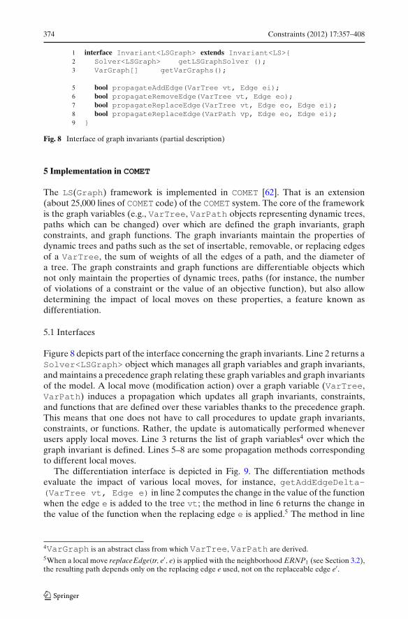
Fig. 8 Interface of graph invariants (partial description)
5 Implementation in COMET
The LS(Graph) framework is implemented in COMET [62]. That is an extension(about 25,000 lines of COMET code) of the COMET system. The core of the frameworkis the graph variables (e.g., VarTree, VarPath objects representing dynamic trees,paths which can be changed) over which are defined the graph invariants, graphconstraints, and graph functions. The graph invariants maintain the properties ofdynamic trees and paths such as the set of insertable, removable, or replacing edgesof a VarTree, the sum of weights of all the edges of a path, and the diameter ofa tree. The graph constraints and graph functions are differentiable objects whichnot only maintain the properties of dynamic trees, paths (for instance, the numberof violations of a constraint or the value of an objective function), but also allowdetermining the impact of local moves on these properties, a feature known asdifferentiation.
5.1 Interfaces
Figure 8 depicts part of the interface concerning the graph invariants. Line 2 returns aSolver<LSGraph> object which manages all graph variables and graph invariants,and maintains a precedence graph relating these graph variables and graph invariantsof the model. A local move (modification action) over a graph variable (VarTree,VarPath) induces a propagation which updates all graph invariants, constraints,and functions that are defined over these variables thanks to the precedence graph.This means that one does not have to call procedures to update graph invariants,constraints, or functions. Rather, the update is automatically performed wheneverusers apply local moves. Line 3 returns the list of graph variables4 over which thegraph invariant is defined. Lines 5–8 are some propagation methods correspondingto different local moves.
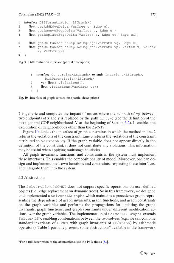
The differentiation interface is depicted in Fig. 9. The differentiation methodsevaluate the impact of various local moves, for instance, getAddEdgeDelta-(VarTree vt, Edge e) in line 2 computes the change in the value of the functionwhen the edge e is added to the tree vt; the method in line 6 returns the change inthe value of the function when the replacing edge e is applied.5 The method in line
4VarGraph is an abstract class from which VarTree, VarPath are derived.5When a local move replaceEdge(tr, e′, e) is applied with the neighborhood ERNP1 (see Section 3.2),the resulting path depends only on the replacing edge e used, not on the replaceable edge e′.
Constraints (2012) 17:357–408 375
Fig. 9 Differentiation interface (partial description)
Fig. 10 Interface of graph constraints (partial description)
7 is generic and computes the impact of moves where the subpath of vp betweentwo endpoints of x and y is replaced by the path 〈x,v,y〉 (see the definition of themost general COP neighborhood N at the beginning of Section 3.2). It enables theexploration of neighborhoods other than the ERNP1.
Figure 10 depicts the interface of graph constraints in which the method in line 2returns the violations of the constraint. Line 3 returns the violations of the constraintattributed to VarGraph vg. If the graph variable does not appear directly in thedefinition of the constraint, it does not contribute any violations. This informationmay be useful when applying multistage heuristics.
All graph invariants, functions, and constraints in the system must implementthese interfaces. This enables the compositionality of model. Moreover, one can de-sign and implement one’s own functions and constraints, respecting these interfaces,and integrate them into the system.
5.2 Abstractions
The Solver<LS> of COMET does not support specific operations on user-definedobjects (i.e., edge replacement on dynamic trees). So in this framework, we designedand implemented a Solver<LSGraph> which maintains a precedence graph repre-senting the dependence of graph invariants, graph functions, and graph constraintson the graph variables and performs the propagations for updating the graphinvariants, graph functions, and graph constraints under different modification ac-tions over the graph variables. The implementation of Solver<LSGraph> extendsSolver<LS>, enabling combinations between the two solvers (e.g., we can combinestandard invariants of COMET with graph invariants of LS(Graph) by arithmeticoperators). Table 1 partially presents some abstractions6 available in the framework
6For a full description of the abstractions, see the PhD thesis [53].

376 Constraints (2012) 17:357–408
Tab
le1
Som
egr
aph
inva
rian
ts,f
unct
ions
and
cons
trai
nts
ofth
efr
amew
ork
(par
tial
desc
ript
ion)
Constraints (2012) 17:357–408 377
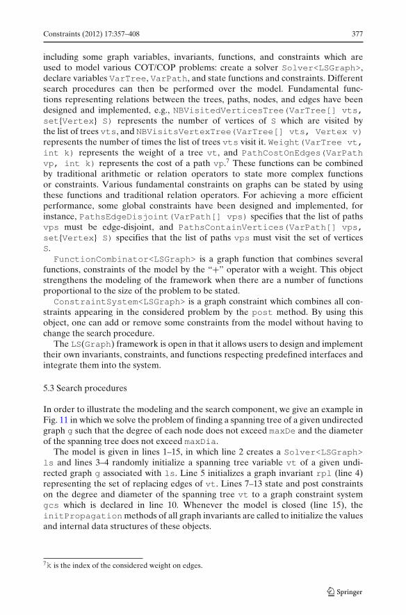
including some graph variables, invariants, functions, and constraints which areused to model various COT/COP problems: create a solver Solver<LSGraph>,declare variables VarTree, VarPath, and state functions and constraints. Differentsearch procedures can then be performed over the model. Fundamental func-tions representing relations between the trees, paths, nodes, and edges have beendesigned and implemented, e.g., NBVisitedVerticesTree(VarTree[] vts,set{Vertex} S) represents the number of vertices of S which are visited bythe list of trees vts, and NBVisitsVertexTree(VarTree[] vts, Vertex v)represents the number of times the list of trees vts visit it. Weight(VarTree vt,int k) represents the weight of a tree vt, and PathCostOnEdges(VarPathvp, int k) represents the cost of a path vp.7 These functions can be combinedby traditional arithmetic or relation operators to state more complex functionsor constraints. Various fundamental constraints on graphs can be stated by usingthese functions and traditional relation operators. For achieving a more efficientperformance, some global constraints have been designed and implemented, forinstance, PathsEdgeDisjoint(VarPath[] vps) specifies that the list of pathsvps must be edge-disjoint, and PathsContainVertices(VarPath[] vps,set{Vertex} S) specifies that the list of paths vps must visit the set of verticesS.FunctionCombinator<LSGraph> is a graph function that combines several
functions, constraints of the model by the “+” operator with a weight. This objectstrengthens the modeling of the framework when there are a number of functionsproportional to the size of the problem to be stated.ConstraintSystem<LSGraph> is a graph constraint which combines all con-
straints appearing in the considered problem by the post method. By using thisobject, one can add or remove some constraints from the model without having tochange the search procedure.
The LS(Graph) framework is open in that it allows users to design and implementtheir own invariants, constraints, and functions respecting predefined interfaces andintegrate them into the system.
5.3 Search procedures
In order to illustrate the modeling and the search component, we give an example inFig. 11 in which we solve the problem of finding a spanning tree of a given undirectedgraph g such that the degree of each node does not exceed maxDe and the diameterof the spanning tree does not exceed maxDia.
The model is given in lines 1–15, in which line 2 creates a Solver<LSGraph>ls and lines 3–4 randomly initialize a spanning tree variable vt of a given undi-rected graph g associated with ls. Line 5 initializes a graph invariant rpl (line 4)representing the set of replacing edges of vt. Lines 7–13 state and post constraintson the degree and diameter of the spanning tree vt to a graph constraint systemgcs which is declared in line 10. Whenever the model is closed (line 15), theinitPropagationmethods of all graph invariants are called to initialize the valuesand internal data structures of these objects.
7k is the index of the considered weight on edges.

378 Constraints (2012) 17:357–408
Fig. 11 Model for bounded diameter and degree constrained spanning tree
The search is given in lines 17–26, which is a simple greedy search. At eachiteration, we explore the NT3 neighborhood and choose the best neighbor w.r.t. thegraph constraint system gcs: we choose a replacing edge ei and a replaceable edgeeo of ei such that the number of violations of gcs is most reduced when eo isreplaced by ei (see method getReplaceEdgeDelta(vt,eo,ei)). Line 23 is thelocal move which induces automatically a propagation to update all graph invariantsand constraints defined over it (e.g., rpl, degreeC, diameterC) thanks to theprecedence graph maintained in ls.
We can see in this example that the model and the search are independent. Onthe one hand, we can state and post other constraints to the graph constraint systemgcs without having to change the search. On the other hand, we can apply differentheuristic local searches in the search component without changing the model.
We now describe one of generic neighborhood explorations. Figure 12 explorethe basic COP neighborhood ERNP1. The quality of a solution is evaluated interms of the number of violations of the Constraint<LSGraph> c. Variablesit and fgb represent the current iteration of the local search and the smallestvalue of the number of violations of the constraint c found so far. All VarPathvps[j] are scanned (lines 7–8). Line 9 retrieves the Invariant<LSGraph> replrepresenting the set of preferred replacing edges of vps[j]. All preferred replacingedges e are scanned in line 10 and line 11 evaluates the quality of the move when

Constraints (2012) 17:357–408 379
Fig. 12 Exploring the ERNP1 neighborhood

380 Constraints (2012) 17:357–408
applying the replacing edge e in term of the variation of the number of violationsof c. Line 13 checks whether e is tabu or the aspiration criterion is reached (i.e.,the move is tabu but it improves the best solution found so far). Lines 31–33 choosea preferred replaceable sel_eo. Lines 36–41 submit a move (lines 36–41) and itsevaluation eval to a Neighborhood N and it will be called later.
Components for a generic tabu search, TabuSearch<LSGraph>, and a greedylocal search, GreedyLocalSearch<LSGraph>, have been implemented forCOT/COP applications. This tabu search component features aspiration criteria withadaptive tabu length (the tabu length can be changed within tb Min and tb Max,depending on the behavior of the search). A full description of the abstractions andgeneric search components can be found in [53].
6 Applications
In this section, we present the application of the LS(Graph) framework to theresolution of three COT/COP problems: the quorumcast routing (QR) problem, theedge-disjoint paths (EDP) problem, and the routing and wavelength assignment withside constraint (RWA-D) problem.
For the first and the third applications (QR and RWA-D), we apply tabu search.Two parameters of tabu search are the length tbl of the tabu lists and maxStable: ifthe best-restart solution8 does not improve in maxStable successive local moves, thenthe search is restarted.
Experiments were performed on XEN virtual machines with 1 core of a CPU IntelCore2 Quad Q6600 @2.40 GHz and 1 GB of RAM.
6.1 The quorumcast routing (QR) problem
6.1.1 Problem statement
Given a weighted undirected graph G = (V, E), each edge e ∈ E is associated with acost w(e). Given a source node r ∈ V, an integral value q, and a set S ⊆ V of multicastnodes, the quorumcast routing problem is to find a minimum cost tree T = (V ′, E′)of G spanning r and q nodes of S. T = (V ′, E′) is a graph satisfying
1. V ′ ⊆ V ∧ E′ ⊆ E,2. T is connected,3. ∃Q ⊆ S such that �Q = q ∧ Q ∪ {r} ⊆ V ′,4. The cost of
T =∑
e∈E′w(e)
is minimum over all subgraphs of G with properties 1–3.
In this section, we present a local search model for solving the QR problem withLS(Graph).
8The best-restart solution is the best solution found for each restart.

Constraints (2012) 17:357–408 381
6.1.2 The model
We propose a tabu search model in LS(Graph) exploring different neighborhoodsfor solving this problem. The model is given in Fig. 13, in which line 1 creates aSolver<LSGraph> and line 2 declares a VarTree tr associated with ls. Lines4–7 state the constraints of the problem where NBVisitedVertices(tr,S) isa Function<LSGraph> representing the number of vertices of S which are inthe tree tr. The constraint posted in line 5 says that the tree tr must contain atleast q vertices of S and the constraint posted in line 6 says that tr must containthe vertex s. Line 9 creates a Model<LSGraph> mod with only one variable tr,the constraint gcs, the objective function to be minimized is the total weight oftr. Line 11 initializes a search component which extends TabuSearch<LSGraph>(see Fig. 14). Lines 12–14 set parameters for the search and line 16 calls the searchprocedure. We now describe the search component in Fig. 14. The variables _cardand _root represent the number of edges of the initial tree and its root computedin the initSolution method. The overriding initSolution method (lines 17–31) constructs the tree in a greedy random way. It clears the tree tr (line 22) andselects randomly a first edge containing _root (lines 23–25). It then iterativelyselects an edge with minimal weight for adding to the constructed tree tr (lines27–30). The exploreNeighborhood method of TabuSearch<LSGraph> is alsooverriden (lines 34–39) with different neighborhoods: NT1 (line 35), NT2 (line 36),NT1+2 (line 37), and NT3 (line 38).
Fig. 13 Tabu search model for the QR problem

382 Constraints (2012) 17:357–408
Fig. 14 The search component for the QR problem

Constraints (2012) 17:357–408 383
6.1.3 Experiments
We compare our tabu model in LS(Graph) with the IMP heuristic, which is the bestheuristic among the three heuristic algorithms in [24]. The original instances and theimplementation of the IMP algorithm are not available. We thus re-implemented theIMP algorithm in COMET and generated new benchmarks.
Problem instances We take six graphs from the benchmark of the KCT problem[20] which are 4-regular graphs of sizes from 50 to 1,000 nodes and six graphs fromthe Steiner tree instances. For each graph of size n, we generate randomly n ∗ tau1
nodes for the set S, the value for q is set to n ∗ tau1 ∗ tau2 with tau1, tau2 ∈ {0.2, 0.5},and the root is set to be node 1.
Results The IMP algorithm and our model in LS(Graph) are executed 20 times foreach problem instance. The time limit for our model is 30 min. From our preliminaryresults, we set tbl to 5 and maxStable to 200. The experimental results are shownin Tables 2 and 3. Columns 3–6 present the average, the minimal, the maximal, andthe standard deviation of the best objective value found in 20 executions. The sameinformation for our model is presented in columns 8–11. Column 7 is the averageexecution time (in seconds) of the IMP algorithm over 20 executions, while column12 presents the average time (in seconds) for finding the best solutions over 20executions of our tabu search model. Table 2 shows that for KCT instances, ourLS(Graph) model finds better solutions than the IMP on average. Moreover, theworst solutions found by our model are, in most cases, even better than the bestsolution found by the IMP (among 20 executions). Table 3 shows that the resultsfound by our model are better than those found by the IMP algorithm on averageexcept for the last four instances (45–48). A comparison of the two algorithms interms of box-and-whiskers plots (see their template presentation in Fig. 15) can befound in Figs. 16, 17, 18, and 19. Two consecutive bars present the results computedby the IMP and the tabu search algorithms on a given instance. The figures show thatfor each algorithm, the variance of the results among the 20 executions is small. Italso shows that, in most instances, the solutions found by our tabu search are betterthan those found by the IMP algorithm.
6.2 The edge-disjoint paths problem
6.2.1 Problem statement
We are given an undirected graph G = (V, E) and a set T = {〈si, ti〉 | i =1, 2, ..., �T; si = ti ∈ V} representing a list of commodities. A subset T ′ ⊆ T, T ′ ={〈si1 , ti1〉, ..., 〈sik , tik〉} is called edp-feasible if there exist mutually edge-disjoint pathsfrom si j to ti j on G, ∀ j = 1, 2, .., k. The EDP problem consists in finding a maximalcardinality edp-feasible subset of T. In other words,
max �T ′ (1)
s.t. T ′ ⊆ T (2)
T ′ is edp-feasible (3)

384 Constraints (2012) 17:357–408
Tab
le2
Exp
erim
enta
lres
ults
onK
CT
inst
ance
s
Inde
xIn
stan
ces
IMP
LS(
Gra
ph)
avg
min
max
std_
dev
avg_
tav
gm
inm
axst
d_de
vav
g_t
1g5
0_20
_20
111
111
111
00.
7811
111
111
10
0.06
2g5
0_20
_50
251
251
251
00.
7824
824
824
80
0.08
3g5
0_50
_20
169
169
169
00.
816
916
916
90
0.09
4g5
0_50
_50
386
386
386
00.
7636
936
936
90
0.22
5g7
5_20
_20
9393
930
1.06
9393
930
0.02
6g7
5_20
_50
358
358
358
01.
0632
832
832
80
1.12
7g7
5_50
_20
207
207
207
01.
0517
517
517
50
0.08
8g7
5_50
_50
630
630
630
01.
0556
4.6
560
568
3.56
181.
819
g100
_20_
2017
817
817
80
1.44
178
178
178
00.
2310
g100
_20_
5052
652
652
60
1.45
524
524
524
02.
3111
g100
_50_
2029
429
429
40
1.51
273
273
273
00.
2812
g100
_50_
5094
894
894
80
1.53
854
854
854
036
.84
13g2
00_2
0_20
428
428
428
07.
1340
240
240
20
32.6
14g2
00_2
0_50
926
926
926
07.
0784
9.6
849
851
0.92
342.
4915
g200
_50_
2048
348
348
30
7.26
468
468
468
08.
0916
g200
_50_
501,
499
1,49
91,
499
07.
351,
411.
451,
403
1,42
45.
8281
6.43
17g4
00_2
0_20
599
599
599
052
.18
556.
655
156
01.
8824
0.46
18g4
00_2
0_50
1,72
4.05
1,70
21,
739
13.9
251
.43
1,61
0.95
1,60
01,
626
7.05
689.
3319
g400
_50_
201,
154.
551,
140
1,16
67.
7551
.61,
010.
651,
005
1,01
84.
358
4.08
20g4
00_5
0_50
3,04
03,
040
3,04
00
52.1
92,
829.
152,
799
2,85
617
.25
845.
5221
g100
0_20
_20
1,83
2.1
1,81
01,
836
9.28
812.
611,
568.
651,
505
1,62
127
.67
584.
7522
g100
0_20
_50
4,76
2.2
4,75
54,
771
7.96
795.
644,
493.
554,
406
4,59
949
.986
9.09
23g1
000_
50_2
02,
743
2,73
32,
746
4.29
801.
062,
487.
22,
429
2,53
327
.04
697.
8524
g100
0_50
_50
7,29
3.85
7,22
97,
361
36.2
881
7.82
7,09
8.95
6,89
17,
372
117.
061,
330.
21

Constraints (2012) 17:357–408 385
Tab
le3
Exp
erim
enta
lres
ults
onst
eine
rin
stan
ces
Inde
xIn
stan
ces
IMP
LS(
Gra
ph)
avg
min
max
std_
dev
avg_
tav
gm
inm
axst
d_de
vav
g_t
25st
einb
4_20
_20
1111
110
0.72
1111
110
026
stei
nb4_
20_5
032
3232
00.
7532
3232
00.
1227
stei
nb4_
50_2
020
.35
2021
0.48
0.74
2020
200
0.08
28st
einb
4_50
_50
52.2
551
530.
770.
7441
4141
00.
2729
stei
nb10
_20_
2019
1919
01
1919
190
0.12
30st
einb
10_2
0_50
2929
290
0.98
2929
290
0.32
31st
einb
10_5
0_20
27.8
2629
1.25
1.03
2222
220
0.16
32st
einb
10_5
0_50
6565
650
0.99
6565
650
2.76
33st
einb
16_2
0_20
1010
100
1.46
1010
100
0.01
34st
einb
16_2
0_50
73.3
569
762.
331.
5561
6161
09.
4635
stei
nb16
_50_
2032
.85
3237
1.19
1.47
3131
310
0.93
36st
einb
16_5
0_50
87.2
585
922.
091.
4882
8282
012
.637
stei
nc6_
20_2
092
.35
8198
4.75
100.
5869
.769
720.
951
4.06
38st
einc
6_20
_50
234.
1522
924
03.
6110
1.77
221.
921
822
51.
7361
4.34
39st
einc
6_50
_20
130.
9512
214
76.
1699
.82
115.
911
311
81.
0937
2.27
40st
einc
6_50
_50
399.
5539
540
73.
1710
3.59
381.
5537
438
73.
2886
6.87
41st
einc
11_2
0_20
43.9
540
471.
9910
2.08
38.7
3839
0.46
481.
5242
stei
nc11
_20_
5011
611
311
91.
5510
2.6
107.
410
710
90.
5880
3.34
43st
einc
11_5
0_20
75.0
570
792.
4810
1.89
67.7
567
690.
6245
544
stei
nc11
_50_
5020
7.25
201
213
2.9
102.
0420
2.45
199
208
2.31
1,00
0.79
45st
einc
16_2
0_20
22.2
521
251.
1310
0.2
23.6
2224
0.66
200.
746
stei
nc16
_20_
5054
.45
5259
1.66
100.
2254
.95
5356
0.74
267.
0147
stei
nc16
_50_
2050
5050
099
.34
50.3
5052
0.56
451
48st
einc
16_5
0_50
125
125
125
010
4.98
140.
2513
314
84.
091,
567.
46

386 Constraints (2012) 17:357–408
Fig. 15 Box-and-Whiskersplot: the X-axis represents thealgorithm and the instance (Adenotes the algorithm and insdenotes the instance) and theY-axis represents the value ofthe objective function
Fig. 16 Comparison betweenIMP and LS(Graph) on KCTinstances
Fig. 17 Comparison betweenIMP and LS(Graph) on KCTinstances

Constraints (2012) 17:357–408 387
Fig. 18 Comparison betweenIMP and LS(Graph) on steinerinstances
Fig. 19 Comparison betweenIMP and LS(Graph) on steinerinstances
In this section, we propose two algorithms based on neighborhood search forsolving the EDP problem by LS(Graph). They are complex heuristics which makeuse of local search in LS(Graph) as sub-routines. We first describe the simple greedyalgorithm SGA [42] because one of our algorithms (detailed later) will apply this assub-procedure (see Algorithm 3).

388 Constraints (2012) 17:357–408
6.2.2 The simple greedy algorithm
This algorithm starts with an empty solution S (line 1). At each iteration j (line 3),it selects a pair T j = 〈s j, t j〉 and tries to find the shortest path Pj from s j to t j in thegraph G1 = (V, E1), initializing the set of edges E1 to be E (line 2). If such a pathexists, it is inserted into S and the set E1 is updated for the next step by removing alledges of the path Pj.
Obviously, the SGA algorithm depends strongly on the order of commoditiesT j considered. The multi-start version of SGA (called MSGA) performs SGAiteratively with different orders of T j to be scanned in T.
In the ACO algorithm of [18], the following criterion is introduced, which quan-tifies the degree of non-disjointness of a solution. S = {P1, P2, ...Pk} (Pj is a pathfrom s j to t j):
C(S) =∑
e∈E
⎛
⎝max{0,∑
P j∈S
ρ j(S, e) − 1}⎞
⎠ ,
where ρ j(S, e) = 1 if e ∈ Pj, and ρ j(S, e) = 0 otherwise. From a solution constructedby ANTs, a solution to the EDP problem is extracted by iteratively removing thepath which has the most edges in common with other paths, until all remaining pathsare mutually edge-disjoint (see Algorithm 4).
In this section, we propose two algorithms based on local search for solvingthis problem: the LS-SGA and the LS-R algorithms. These algorithms performa local search procedure applying the LS(Graph) framework combined with theextraction method (Algorithm 4) and the simple greedy algorithm. These algorithmsmake use of the PathsEdgeDisjoint(P1, P2, ..., Pk) constraint of the LS(Graph)framework saying that the set of paths {P1, P2, ..., Pk} must be edge-disjoint. Thenumber of violations of the PathsEdgeDisjoint(P1, P2, ..., Pk) constraint is definedto be C({P1, P2, ..., Pk}) and the local search algorithms used in our heuristics try tominimize this number.
6.2.3 The LS-SGA algorithm
The LS-SGA algorithm has been proposed in our paper [54]. The main ideaof the LS-SGA algorithm (given in detail in Algorithm 5) is to perform alocal search algorithm aiming at minimizing the number of violations of thePathsEdgeDisjoint(P1, P2, ..., Pk) constraint. The variable S (line 2) stores a setof paths {P1, P2, ..., Pk} connecting all commodities. It is initialized randomly (lines

Constraints (2012) 17:357–408 389
3–5). At each step, we perform a local move. The LocalMove method (line 7)returns true if it finds a move that decreases the number of violations of thePathsEdgeDisjoint(P1, P2, ..., Pk) constraint. If no such move exists, we make somerandom moves (line 22). From a candidate solution S found by the local search, asolution S1 to the EDP problem will be extracted by applying the Extract algorithm(line 9) combined with the SGA algorithm (line 15) on the remaining graph G′′ (thegraph G′′ is obtained by removing all edges E′ (line 12) of the paths extracted bythe Extract algorithm) and the remaining commodities T ′′ (lines 10 and 11). The bestsolution is updated in line 17 and lines 18–20 update some paths of S by the newfound paths of S2.
6.2.4 The LS-R algorithm
The idea is to connect recursively as much as possible the commodities of T (seeAlgorithm 6). The core is the recursive method LS-Recursive in Algorithm 7, whichreceives a graph G and a list of commodities T as input and computes a set ofmaximally edge-disjoint paths connecting the commodities of T. This paths set isthen accumulated in the solution Sol (Sol is a global variable) and all edges visitedby these paths are removed from G for the next recursive call. Line 1 computes a setof edge-disjoint paths by a greedy local search method, GreedyLocalSearch. Lines2–3 update the solution by adding the new found edge-disjoint paths of Si. Lines3–4 compute the set of connected components CC of the graph generated from thecurrent graph by removing all edges E′ of paths of Si. For each graph Gi of these

390 Constraints (2012) 17:357–408
connected components and each set of commodities Ti that belong to Gi, we performrecursively the LS-Recursive method (see lines 6–8).
The implementation of these algorithms in LS(Graph) is given in the PhD thesis[53]. It is more complicated than that of the QR problem: it requires some processing(e.g., removing edges and vertices from a graph, and computing the connectedcomponents of a graph) other than just stating the model and performing the search.
6.2.5 Experiments
Problem instances We tried the two proposed algorithms on three types of bench-mark. The first benchmark contains instances on four graphs provided by Blesa [18].The second benchmark contains instances on some graphs of the Steiner benchmarkfrom the Or-Library [14]. The third benchmark consists of instances on randomplanar graphs. Table 4 gives a description of these graphs.
An instance of the EDP problem consists of a graph and a set of commodities. Theinstances in the original paper [18] are not available. As a result, we base our trialon the instance generator described in [18] and generate new instances as follows.For each graph of the first set, we generate randomly different sets of commoditieswith different sizes, depending on the size of the graph: for each graph of size n, wegenerate randomly two instances9 with 0.10*n, 0.25*n, and 0.40*n commodities. Wedo the same for each Steiner and planar graph but we generate only one instance for
9This is different from what we did in [54], where we randomly generated 20 instances for each rateof commodity. For each instance, the algorithm was executed only once.

Constraints (2012) 17:357–408 391
Table 4 Description of graphsof the benchmarks
Name |V| |E| Degree avg.
bl-wr2-wht2.10-50.rand 500 1,020 4.08bl-wr2-wht2.10-50.sdeg 500 1,020 4.08mesh15×15 225 420 3.73mesh25×25 625 1,200 3.84steinb4.txt 50 100 4.00steinb10.txt 75 150 4.00steinb16.txt 100 200 4.00steinc6.txt 500 1,000 4.00steinc11.txt 500 2,500 10.00steinc16.txt 500 12,500 50.00planar-n50 50 135 5.4planar-n100 100 285 5.7planar-n200 200 583 5.83planar-n500 500 1,477 5.91
each rate of commodity instead of two. Table 5 describes the instances generated,including their numbers of vertices, edges, and the sizes of the commodity sets T.
For comparison, we have reimplemented the ACO algorithm described in [18] inthe COMET programming language. For each problem instance, the three algorithmsACO, LS-SGA, and LS-R are executed 20 times each. Due to the high complexity ofthe problem, we set the time limit to 30 min for each execution. In total, we have 54problem instances and 1,080 executions.
Results The experimental results are shown in Tables 6, 7 and 8. These tables havethe same structure, which is described in what follows. The first column presents theinstance name. Columns 2–5 present the results of the ACO algorithm [18], includingthe average, the minimal and the maximal of the best objective values found in 20executions, and the average time for finding these best objective values. The sameinformation for LS-SGA and LS-R are presented in columns 6–9 and columns 11–14. Column 10 compares the ACO and LS-SGA algorithms in the format a/b wherea is the number of times the ACO algorithm found better solutions than the LS-SGA algorithm and b is the number of time the LS-SGA found better solutionsthan the ACO algorithm in 20 executions. Column 15 presents the same informationas column 10 but for the comparison between the ACO and the LS-R algorithms.A comparison of the two algorithms in terms of box-and-whiskers plots (see theirtemplate presentation in Fig. 15) can be found in Figs. 20, 21, 22, 23, 24, and 25.Three consecutive bars present the results computed by the ACO, LS-SGA, and theLS-R algorithms on a given instance. The figures show that for each algorithm, the
Table 5 Description of instances
Index Name �V �E �T
1 bl-wr2-wht2.10-50.rand.bb_com10_ins1 500 1,020 502 bl-wr2-wht2.10-50.rand.bb_com25_ins1 500 1,020 1253 bl-wr2-wht2.10-50.rand.bb_com40_ins1 500 1,020 2004 bl-wr2-wht2.10-50.rand.bb_com10_ins2 500 1,020 505 bl-wr2-wht2.10-50.rand.bb_com25_ins2 500 1,020 1256 bl-wr2-wht2.10-50.rand.bb_com40_ins2 500 1,020 2007 bl-wr2-wht2.10-50.sdeg.bb_com10_ins1 500 1,020 50

392 Constraints (2012) 17:357–408
Table 5 (continued)
Index Name �V �E �T
8 bl-wr2-wht2.10-50.sdeg.bb_com25_ins1 500 1,020 1259 bl-wr2-wht2.10-50.sdeg.bb_com40_ins1 500 1,020 20010 bl-wr2-wht2.10-50.sdeg.bb_com10_ins2 500 1,020 5011 bl-wr2-wht2.10-50.sdeg.bb_com25_ins2 500 1,020 12512 bl-wr2-wht2.10-50.sdeg.bb_com40_ins2 500 1,020 20013 mesh15×15.bb_com10_ins1 225 420 2214 mesh15×15.bb_com25_ins1 225 420 5615 mesh15×15.bb_com40_ins1 225 420 9016 mesh15×15.bb_com10_ins2 225 420 2217 mesh15×15.bb_com25_ins2 225 420 5618 mesh15×15.bb_com40_ins2 225 420 9019 mesh25×25.bb_com10_ins1 625 1,200 6220 mesh25×25.bb_com25_ins1 625 1,200 15621 mesh25×25.bb_com40_ins1 625 1,200 25022 mesh25×25.bb_com10_ins2 625 1,200 6223 mesh25×25.bb_com25_ins2 625 1,200 15624 mesh25×25.bb_com40_ins2 625 1,200 25025 steinb4.txt_com10_ins1 50 100 526 steinb4.txt_com25_ins1 50 100 1227 steinb4.txt_com40_ins1 50 100 2028 steinb10.txt_com10_ins1 75 150 729 steinb10.txt_com25_ins1 75 150 1830 steinb10.txt_com40_ins1 75 150 3031 steinb16.txt_com10_ins1 100 200 1032 steinb16.txt_com25_ins1 100 200 2533 steinb16.txt_com40_ins1 100 200 4034 steinc6.txt_com10_ins1 500 1,000 5035 steinc6.txt_com25_ins1 500 1,000 12536 steinc6.txt_com40_ins1 500 1,000 20037 steinc11.txt_com10_ins1 500 2,500 5038 steinc11.txt_com25_ins1 500 2,500 12539 steinc11.txt_com40_ins1 500 2,500 20040 steinc16.txt_com10_ins1 500 12,500 5041 steinc16.txt_com25_ins1 500 12,500 12542 steinc16.txt_com40_ins1 500 12,500 20043 planar-n50.ins1.txt_com10_ins1 50 135 544 planar-n50.ins1.txt_com25_ins1 50 135 1245 planar-n50.ins1.txt_com40_ins1 50 135 2046 planar-n100.ins1.txt_com10_ins1 100 285 1047 planar-n100.ins1.txt_com25_ins1 100 285 2548 planar-n100.ins1.txt_com40_ins1 100 285 4049 planar-n200.ins1.txt_com10_ins1 200 583 2050 planar-n200.ins1.txt_com25_ins1 200 583 5051 planar-n200.ins1.txt_com40_ins1 200 583 8052 planar-n500.ins1.txt_com10_ins1 500 1,477 5053 planar-n500.ins1.txt_com25_ins1 500 1,477 12554 planar-n500.ins1.txt_com40_ins1 500 1,477 200
variance of the results among the 20 executions is small. It also shows that, in mostinstances, the solutions found by LS-SGA and LS-R are better than those found bythe ACO algorithm.

Constraints (2012) 17:357–408 393
Tab
le6
Exp
erim
enta
lres
ults
ofth
efi
rstg
raph
sse
t
Ins.
AC
OL
S-SG
AL
S-R
fm
Mt
fm
Mt
τ 1f
mM
tτ 2
114
.814
1613
1.6
15.6
1416
410.
762/
1316
1616
194.
710/
192
31.8
531
3216
5.22
31.4
3032
564.
9910
/332
3232
263.
710/
33
37.8
537
3821
9.56
37.6
3638
322.
966/
237
.937
3823
0.29
1/2
425
.25
2526
95.4
125
.925
2643
4.43
0/13
2626
2615
1.09
0/15
534
.75
3435
97.3
334
.432
3554
4.02
8/4
34.9
534
3530
3.26
0/4
636
.95
3637
185.
1436
.05
3437
422.
1813
/036
.95
3637
293.
271/
17
15.9
515
1689
.24
16.2
516
1752
9.03
0/6
1717
1743
0.99
0/20
835
.835
3667
.08
35.4
534
3653
6.4
8/3
3636
3642
3.68
0/4
933
.65
3334
169.
933
.131
3447
2.56
11/4
3434
3455
7.57
0/7
1019
.219
2040
1.19
19.6
519
2052
2.22
2/11
2020
2044
8.59
0/16
1132
.95
3234
365.
0932
.931
3488
0.04
9/7
33.9
3334
516.
211/
1412
36.5
3537
133
35.7
3537
936.
5711
/237
3737
583.
990/
913
19.6
519
2145
7.46
21.7
521
2264
4.11
0/20
21.5
521
2236
0.53
0/19
1427
.726
2947
0.98
29.8
2931
335.
510/
1932
3133
887.
930/
2015
35.3
3238
871.
2235
.833
3976
3.25
6/10
38.8
3740
960.
970/
2016
17.5
1719
479.
8919
.419
2051
5.65
0/19
19.4
519
2056
8.74
0/18
1729
.228
311,
010.
5231
.730
3348
0.98
0/20
33.0
532
3459
2.96
0/20
1834
3336
750.
5534
.633
3764
9.26
4/13
37.6
3639
910.
630/
2019
32.8
529
3699
6.96
39.1
536
4186
4.6
0/20
4139
4394
6.47
0/20
2045
4249
1,10
4.82
51.9
549
561,
053.
570/
2055
.55
5459
1,11
1.8
0/20
2157
.753
6179
7.14
65.3
6069
950.
870/
2069
.367
721,
520.
610/
2022
30.1
2833
944.
3635
.734
3787
5.12
0/20
37.9
3640
945.
080/
2023
45.6
4448
1,01
5.84
51.3
547
5467
3.59
0/20
54.7
5259
1,04
2.11
0/20
2457
.75
5461
939.
8265
.05
6268
1,40
9.13
0/20
68.8
566
711,
040.
240/
20

394 Constraints (2012) 17:357–408
Tab
le7
Exp
erim
enta
lres
ults
ofth
est
eine
rgr
aphs
set
Ins.
AC
OL
S-SG
AL
S-R
fm
Mt
fm
Mt
τ 1f
mM
tτ 2
255
55
0.01
55
51.
120/
05
55
1.09
0/0
2612
1212
0.44
1212
121.
220/
012
1212
1.4
0/0
2720
2020
51.1
120
2020
5.45
0/0
19.9
1920
2.8
2/0
287
77
0.02
77
71.
350/
07
77
1.16
0/0
2917
.85
1718
96.4
818
1818
13.4
20/
318
1818
5.2
0/3
3024
.35
2326
242.
0426
.25
2627
682.
840/
2027
.327
2850
5.22
0/20
3110
1010
0.25
1010
101.
460/
010
1010
1.52
0/0
3224
.35
2425
364.
9925
2525
93.5
30/
1325
2525
8.86
0/13
3332
.45
3234
658.
2534
.133
3674
7.34
0/19
35.9
535
3764
6.19
0/20
3449
.147
5057
2.75
5050
5018
4.44
0/12
5050
5024
0.75
0/12
3589
.985
9472
8.76
92.2
8710
073
4.88
4/12
104.
9510
210
81,
370.
880/
2036
109.
810
611
792
4.1
112.
0510
611
897
1.4
2/14
121.
411
912
51,
372.
370/
2037
5050
5023
.59
5050
5042
.19
0/0
5050
5037
.64
0/0
3812
3.3
122
125
521.
812
512
512
512
8.49
0/17
125
125
125
262.
380/
1739
194.
2519
019
849
4.64
200
200
200
395.
540/
2020
020
020
047
3.81
0/20
4050
5050
6.89
5050
5055
.12
0/0
5050
5046
.01
0/0
4112
512
512
517
.13
125
125
125
194.
360/
012
512
512
511
3.83
0/0
4220
020
020
045
.32
200
200
200
366.
690/
020
020
020
018
3.32
0/0

Constraints (2012) 17:357–408 395
Tab
le8
Exp
erim
enta
lres
ults
ofth
epl
anar
grap
hsse
t
Ins.
AC
OL
S-SG
AL
S-R
fm
Mt
fm
Mt
τ 1f
mM
tτ 2
435
55
0.03
55
50.
860/
05
55
0.8
0/0
4412
1212
0.16
1212
120.
960/
012
1212
0.97
0/0
4520
2020
36.3
820
2020
25.1
20/
019
.919
2031
.18
2/0
4610
1010
0.12
1010
101.
140/
010
1010
1.07
0/0
4725
2525
20.2
225
2525
7.05
0/0
2525
255.
330/
048
3433
3668
0.72
35.3
3437
813.
560/
1636
3537
698.
880/
1849
2020
2013
.46
2020
204.
060/
020
2020
5.23
0/0
5041
.839
4388
9.07
44.8
543
4798
8.81
0/20
45.9
545
4885
3.18
0/20
5149
.35
4751
790.
6553
.35
5156
1,03
3.97
0/19
55.7
5458
901.
740/
2052
44.9
542
471,
100.
4149
.95
4950
484.
840/
2050
5050
309.
240/
2053
60.9
557
6595
4.35
73.8
570
771,
345.
740/
2078
.277
801,
044.
030/
2054
82.8
578
8612
35.1
393
.95
9199
1,36
6.27
0/20
100.
1597
102
1,45
5.43
0/20

396 Constraints (2012) 17:357–408
Fig. 20 Comparison between the ACO, LS-SGA and LS-R algorithms (part I)
The experiments results show that on average, the LS-R algorithm is better thantwo other algorithms. The LS-SGA algorithm is better than the ACO algorithm. TheLS-SGA finds better solutions than the ACO algorithm in 534 out of 1,080 executionswhile the ACO algorithm finds better solutions in 96 out of 1,080 executions. LS-R finds better solutions than ACO in 614 out of 1,080 executions while the ACOalgorithm finds better solutions than LS-R in 7 out of 1,080 executions.
Fig. 21 Comparison between the ACO, LS-SGA and LS-R algorithms (part II)

Constraints (2012) 17:357–408 397
Fig. 22 Comparison between the ACO, LS-SGA and LS-R algorithms (part III)
6.3 The routing and wavelength assignment problem with delay side constraint(RWA-D)
The last application demonstrates that VarPath variables of LS(Graph) andvar{int} of COMET can easily be combined.
6.3.1 Problem statement
Given an undirected weighted graph G = (V, E), each edge e of G has costc(e) (e.g., the delay in traversing e). Suppose given a set of connection requests
Fig. 23 Comparison between the ACO, LS-SGA and LS-R algorithms (part IV)

398 Constraints (2012) 17:357–408
Fig. 24 Comparison between the ACO, LS-SGA and LS-R algorithms (part V)
R = {〈s1, t1〉, 〈s2, t2〉, ..., 〈sk, tk〉} and a value D. The RWA-D problem consists offinding routes pi from si to ti and their wavelengths for all i = 1, 2, ..., k such that:
1. the wavelengths of pi and pj are different if they have common edges, ∀i = j ∈{1, 2, ..., k} (wavelength constraint),
2.∑
e∈pic(e) ≤ D,∀i = 1, 2, ..., k (delay constraint),
3. the number of different wavelengths is minimized (objective function).
6.3.2 The model
The idea of the proposed algorithm is simple. We iteratively perform a local searchalgorithm for finding a feasible solution to the RWA-D problem with W wavelengths(W = 1, 2, 3, ...) until the first feasible solution is discovered.
Fig. 25 Comparison between the ACO, LS-SGA and LS-R algorithms (part VI)

Constraints (2012) 17:357–408 399
The model is given in Fig. 26. Lines 4–10 initialize all VarPath vps[i] froms[i] to t[i] with the shortest version. Line 11 initializes an array vw wherevw[i] stores the wavelength value for the path vps[i]. The search starts with onewavelength (see line 14). At each step, we try to find a feasible solution to the RWA-D problem by a localsearch procedure (line 16). The search terminates (line 17)if a feasible solution to the RWA-D problem is discovered, otherwise, we increase Wby one (line 19).
The localsearch procedure described in Fig. 27 receives an array of VarPath,a value W of the number of wavelengths, and local search parameters maxIt andmaxT as input. Line 2 creates a Solver<LSGraph> ls and lines 4–6 post allVarPath to it. Line 8 initializes an array var{int} xw, where xw[i] representsthe wavelength assigned to the path vps[i] and is initialized with the valuevw[i]. The domain of xw[i] is 1..W. Line 10 initializes a ConstraintSystem<LSGraph> CS. The first constraint of the RWA-D problem is stated and posted inline 12. Lines 14 and 15 state and post all side constraints (the delay constraint) toCS and line 17 closes the constraint system CS. Line 19 groups all variables vps, xw,and the constraint CS, into a model mod. Line 20 creates a search component whichwill be given in detail in Fig. 28. Lines 22 and 23 set parameters for the search andline 25 performs the search. The value of xw is stored in vw for the next iteration (seelines 27 and 28): all paths vps[i] and their wavelengths xw[i] are conserved forthe next localsearch. The localsearch returns true if a feasible solution tothe RWA-D problem is discovered (lines 30–32).
The search component is given in Fig. 28. It extends the TabuSearch<LSGraph>and receives Lmax (line 3) as parameters for the solution initialization when restart-ing the tabu search. The restartSolution is overriden (lines 13–24) in whichwe initialize the value for the VarPath vps[i] with the shortest version if its
Fig. 26 Model for the RWA-D problem

400 Constraints (2012) 17:357–408
Fig. 27 The local search procedure for the RWA-D problem
cost is greater than Lmax. This aims at quickly satisfying the delay constraint. TheinitSolution is also overriden, which does nothing in order not to change thevalue of the variables computed in the previous step of the search. The search ex-plores two neighborhoods (lines 7–10) (see [53] for details about these neighborhoodexplorations).
6.3.3 Naive greedy algorithm
As far as we know, the RWA-D problem has not been considered before. Inorder to assess the efficiency of our local search, we implement a simple greedyheuristic algorithm for the RWA-D problem (see Algorithm 8). The main idea of

Constraints (2012) 17:357–408 401
Fig. 28 The search component
this greedy heuristic is to find the shortest path10 for each connection request andassigns a wavelength to this connection request in a greedy way without violatingthe wavelength constraint. Variable Sol in line 1 represents the set of paths underconstruction. Variable W (line 2) contains the set of wavelengths used for thepaths which have already been constructed. Variable nb Wavelengths (line 3) is thenumber of wavelengths used. For each connection request 〈si, ti〉 (line 4), we assignthe shortest path Pi to it (line 6). Variable Wi in line 5 represents the candidatewavelengths for Pi. Lines 7–9 remove all impossible wavelengths for Pi from Wi. Ifno wavelength already used is possible for Pi (line 10), then we have to find a newwavelength wi for Pi (lines 11 and 12). If the candidate set Wi is not null, we select
10The shortest path best ensures satisfaction of the delay constraint.

402 Constraints (2012) 17:357–408
randomly a wavelength from Wi and assign it to Pi (line 15). Lines 16 and 17 updatethe solution.
6.3.4 Experiments
We compare our local search model with the naive greedy algorithm described in Al-gorithm 8 (multistart version with 1,000 different orders of 〈si, ti〉 to be considered).
The two algorithms have been tried on different instances (graphs from 16 nodesand 33 edges to 100 nodes and 261 edges and with 10, 20, and 50 connection requestsfor each graph). Due to the complexity of the problem, we set the number ofiterations for the tabu search (the value of maxIt in line 16 of Fig. 26) to 200. Foreach problem instance, the model is executed 20 times. From our preliminary results,we set the length of the tabu lists tbl to 5 and the value of maxStable to 20.
Table 9 shows the experimental results. Column 2 presents the objective valuesfound by the naive greedy algorithm. Columns 3–6 show the minimal, the maximal,and the average of the best objective value found, and the average execution time(in seconds) over 20 runs. The experimental results show that the local search givesbetter solutions than the naive greedy algorithm. Especially when the number ofconnection requests increases (i.e., with 50 connection requests), the results found bythe local search are two or three times better than those found by the naive greedyalgorithm. We can see that the number of wavelengths used increases when thenumber of connection requests increases. Given a number of connection requests,if the size of the graph increases, then the number of wavelengths used decreases dueto the fact that on larger graphs, each link is shared by fewer paths of the solutionfound by the local search and if two paths are completely edge-disjoint, they canbe assigned the same wavelength. For instance, with 50 connection requests, on thegraph of 100 vertices, we needed to use only four wavelengths (line 18), while on thegraph of 16 vertices, we had to use eight wavelengths (line 6).

Constraints (2012) 17:357–408 403
Table 9 Experimental results for the RWA-D problem
Instances Greedy f _ min f _ max f t
arpanet_ca10.ins1 5 2 2 2 2.15arpanet_ca20.ins1 9 6 7 6.05 11.36arpanet_ca50.ins1 16 8 9 8.3 68.35grid_ext_4×4_ca10.ins1 3 2 2 2 1.62grid_ext_4×4_ca20.ins1 9 4 5 4.3 7.16grid_ext_4×4_ca50.ins1 24 8 10 8.55 55.04grid_ext_5×5_ca10.ins1 4 2 2 2 2.43grid_ext_5×5_ca20.ins1 7 2 3 2.95 6.21grid_ext_5×5_ca50.ins1 21 5 8 6.45 54.15grid_ext_6×6_ca10.ins1 3 2 2 2 2.58grid_ext_6×6_ca20.ins1 4 2 3 2.1 6.66grid_ext_6×6_ca50.ins1 20 5 6 5.35 58.99grid_ext_8×8_ca10.ins1 4 2 2 2 3.81grid_ext_8×8_ca20.ins1 9 3 4 3.3 14.61grid_ext_8×8_ca50.ins1 11 4 6 5.15 73.97grid_ext_10×10_ca10.ins1 4 2 4 2.7 9.71grid_ext_10×10_ca20.ins1 8 3 5 4 24.22grid_ext_10×10_ca50.ins1 13 4 6 4.75 105.2
Once again, in the above model, we notice that it is easy to state and post variousbuilt-in COMET constraints over var{int} to the graph constraint system CS, whichshows the flexibility and compositionality of the framework.
7 Conclusion
This paper considered constrained optimum trees and paths (COT/COP) problemswhich arise in many real-life applications. It proposed a domain-specific constraint-based local search (CBLS) framework (called LS(Graph)) for solving COT/COPapplications, enabling models to be high level, compositional, and extensible, andallowing for a clear separation between model and search. The key technical contri-bution to support the COP framework is a novel neighborhood based on a rootedspanning tree that implicitly defines a path between the source and the target andits neighbors, and provides an efficient data structure for differentiation. The paperproved that the neighborhood obtained by swapping edges in this tree is connectedand presented a larger neighborhood involving multiple independent moves. TheLS(Graph) framework, implemented in COMET, was applied to the quorumcastrouting problem, the edge-disjoint paths problem, and the routing and wavelengthassignment problem with side constraints on optical networks. Computational resultsshowed the potential significance of the approach, both from a modeling and acomputational standpoint.
Our future work will focus on the construction of a generic constraint program-ming (CP) framework and a hybrid system combining CP and CBLS for modelingand solving COT/COP problems.
Acknowledgements We would like to thank the reviewers for their helpful comments and sug-gestions. This research is partially supported by the Interuniversity Attraction Poles Programme(Belgian State, Belgian Science Policy) and the FRFC project 2.4504.10 of the Belgian FNRS(National Fund for Scientific Research).

404 Constraints (2012) 17:357–408
Appendix
This appendix presents the proofs of above propositions.
Proof of Proposition 1
Proof The proof is divided into two phases:
1. We show that if the conditions (1) and (2) are satisfied, then pathtr′(s) =pathtr(s).The condition (1) ensures that the selected edge e′ satisfying the condition(2) always exist. It is easy to see that e′ belongs to pathtr(s) and this edge isremoved from that path after taking rep(tr, e′, e). That means e′ does not belongto pathtr′(s). Hence, pathtr′(s) = pathtr(s).
2. We now show that if pathtr′(s) = pathtr(s), then the conditions (1) and (2) aresatisfied.We prove this by refutation. Suppose that su = sv. We denote r = su = sv andr1 = ncatr(u, v). Because r Domtr u and r Domtr v, we have r Domtr ncatr(u, v) =r1 (3).We now show that pathtr(u, v) does not contain any edges that belong topathtr(s).
– If pathtr(u, r1) contains an edge (x, y) (where y = fatr(x)) of pathtr(s), thenwe have x Domtr u and x Domtr s. Hence, x Domtr ncatr(s, u) = r (4).Otherwise, (x, y) ∈ pathtr(u, r1), so r1 Domtr y, and we have r Domtr y(because r Domtr r1) that means r Domtr fatr(x) (5). We see that (4) conflictswith (5). From that, we have the fact that pathtr(u, r1) does not contain anyedges of pathtr(s).
– In the same way we can show that pathtr(v, r1) does not contain any edges ofpathtr(s).
From that, we have pathtr(u, v) which is actually the concatenation ofpathtr(u, r1) and pathtr(v, r1) does not contain any edges of pathtr(s).e′ is a replacable edge that belongs to pathtr(u, v). So after the replacement istaken, no edge of pathtr(s) is removed. Hence, the path from s to the root ofthe tree does not change, that means pathtr′(s) = pathtr(s) (this conflicts with thehypothesis that pathtr′(s) = pathtr(s)). So we have su = sv.We now suppose that e′ (the edge to be removed) does not belong topathtr(su, sv). We can see easily that the path from u to v on tr (pathtr(u, v))is composed by the path from u to su, the path from su to sv and the pathfrom sv to v on tr. So after the replacement is taken, no edge of pathtr(s) isremoved. Hence, pathtr′(s) = pathtr(s) (this conflicts with the hypothesis). So wehave e′ ∈ pathtr(su, sv). ��
Proof of Proposition 2
Proof The proposition is proved by showing how to generate that instance trk. Thiscan be done by Algorithm 9. The idea is to travel the sequence of nodes of P on thecurrent tree tr. Whenever we get stuck (we cannot go from the current node x to thenext node y of P by an edge (x, y) on tr because (x, y) is not in tr), we change tr by

Constraints (2012) 17:357–408 405
replacing (x, y) by a replacable edge of (x, y) that is not traversed. The edge (x, y) inline 7 is a replacing edge of tr because this edge is not in tr but it is an edge of g. Line8 chooses a replacable edge eo of ei that is not in S. This choice is always successfullydone because the set of replacable edges of ei that are not in S is not null (at leastan edge (y, fatr(y)) belongs to this set). Line 9 performs the move that replaces theedge eo by the edge ei on tr. So Algorithm 9 always terminates and returns a rootedspanning tree tr inducing P . Variable S (line 1) stores the set of traversed edges.
��
Proof of Proposition 3
Proof All sequences of these basic moves are executable and the final results havethe same set of edges E(tr) \ {eo1, eo2, ..., eok} ∪ {ei1, ei2, ..., eik}. Thus the result treesof all execution sequences are the same. ��
Proof of Proposition 4
Proof Let x = ncatr(u1, v2), sv1 = ncatr(s, v1), su1 = ncatr(s, u1), sv2 = ncatr(s, v2),su2 = ncatr(s, u2). Because su1 Domtr sv1, sv2 Domtr su1, su2 Domtr sv2, e′
1 belongsto pathtr(sv1, su1) and e′
2 belongs to pathtr(sv2, su2), we have e′1 = e′
2. Otherwise, e2
Dom(tr) e1 and these two edges are not in tr, whereas e′1 and e′
2 are in tr. So e1, e′1, e2, e′
2are all different.We will show that the sequence: rep(tr, e′
1, e1), rep(tr, e′2, e2) is feasible
as follows:Suppose that v′
1, u′1 are endpoints of e′
1 such that u′1 = fatr(v
′1) and let tr1 =
rep(tr, e′1, e1). We have that:
(1) su1 Domtr u′1
(2) su2 Domtr u′1
(3) sv2 Domtr u′1
It is straightfoward to find that Ttr(v′1) does not change after taking rep(tr, e′
1, e1).We can also find that u1, v2, u2 must belong to Ttr(v
′1) (if not, u1, v2, u2
must belong to Ttr(v′1), thus ncatr(s, u1), ncatr(s, v2), ncatr(s, u2) are dominated
by v′1, hence this conflicts with (1)–(3)). Thus ncatr1(s, u2) = ncatr(s, u2) = su2

406 Constraints (2012) 17:357–408
and ncatr1(u1, v2) = ncatr(u1, v2) = x. Moreover, from the Property 1, we havencatr1(s, v2) = ncatr1(u1, v2) = x (4).
Due to the fact that sv2 Domtr1 su1 and su1 Domtr1 u1, we have sv2 Domtr1
u1 (5). From the fact that sv2 Domtr1 v2 and sv2 Domtr1 u1, we have sv2 Domtr1
ncatr1(u1, v2) = x (6). We have e′2 belongs to pathtr(sv2, su2) (7). From (6) and (7)
we have that e′2 belongs to pathtr1(x, su2) (8). From (4) and (8), we have e′
2 ∈pathtr1(ncatr1(s, v2), ncatr1(s, u2). That means e′
2 is still a pref fered replacable edge ofe2 on tr1. So the sequence rep(tr, e′
1, e1), rep(tr, e′2, e2) is feasible.
In similar way, we can prove that the sequence rep(tr, e′2, e2), rep(tr, e′
1, e1) is alsofeasible. Hence, two basic moves rep(tr, e′
1, e1), rep(tr, e′2, e2) are independent. ��
References
1. Acar, U., Blelloch, G., Harper, R., Vittes, J., & Woo, S. (2004). An experimental analysis ofchange propagation in dynamic trees. In Proc 15th SODA (pp. 524–533).
2. Ahuja, R. K., Magnanti, T. L., & Orlin, J. B. (1993). Network f lows: Theory, algorithms, andapplications. Englewood Cliffs: Prentice Hall.
3. Ahuja, R. K., Orlinb, J. B., & Sharma, D. (2003). A composite very large-scale neighborhoodstructure for the capacitated minimum spanning tree problem. Operations Research Letters, 31,185–194.
4. Ali, M., Ramamurthy, B., & Deogun, J. (1999). Genetic algorithm for routing in wdm opticalnetworks with power considerations. Part I: The unicast case. In Proceedings of the 8th IEEEICCCN’99 (pp. 335–340). Boston-Natick, MA, USA.
5. Ali, M., Ramamurthy, B., & Deogun, J. (2000). Routing and wavelength assignment with powerconsiderations in optical networks. Computer Networks, 32, 539–555.
6. Alstrup, S., Holm, J., Lichtenberg, K. D., & Thorup, M. (2005). Maintaining information infully dynamic trees with top trees. ACM Transactions on Algorithms, 1(2), 243–264. doi:10.1145/1103963.1103966.
7. Andrade, R., Lucena, A., & Maculan, N. (2006). Using lagrangian dual information to generatedegree constrained spanning trees. Discrete Applied Mathematics, 154(5), 703–717.
8. Awerbuch, B., Gawlick, R., Leighton, T., & Rabani, Y. (1994). On-line admission control andcircuit routing for high performance computing and communication. In 35th IEEE symposiumon foundations of computer science (FOCS1994) (pp. 412–423).
9. Badeau, P., Gendreau, M., Guertin, F., Potvin, J. Y., & Taillard, E. (1997). A parallel tabu searchheuristic for the vehicle routing problem with time windows. Transportation Research - C, 5,109–122.
10. Banerjee, D., Mehta, V., & Pandey, S. (2004). A genetic algorithm approach for solving therouting and wavelength assignment problem in wdm networks. In 3rd IEEE/IEE internationalconference on networking, ICN’2004 (pp. 70–78). Paris.
11. Banerjee, D., & Mukherjee, B. (2000). Wavelength-routed optical networks: Linear formulation,resource budgeting tradeoffs, and a reconfiguration study. IEEE/ACM Transactions on Network-ing, 8, 598–607.
12. Banerjee, S., Yoo, J., & Chen, C. (1997). Design of wavelength routed optical networks for packetswitched traffic. IEEE Journal of Lightware Technology, 15(9), 1636–1646.
13. Baveja, A., & Srinivasan, A. (2000). Approximation algorithms for disjoint paths and relatedrouting and packing problems. Mathematics of Operations Research, 25(2), 255–280.
14. Beasley, J. E. (2012). Or-library. http://people.brunel.ac.uk/∼mastjjb/jeb/info.html. Accessed 15Nov 2009.
15. Beasley, J. E., & Christofides, N. (1989). An algorithm for the resource constrained shortest pathproblem. Network, 19, 379–394.
16. Bender, M. A., Farach-Colton, M., Pemmasani, G., Skiena, S., & Sumazin, P. (2005). Lowestcommon ancestors in trees and directed acyclic graphs. Journal of Algorithms, 57, 75–94.
17. Berkman, O., & Vishkin, U. (1993). Recursive star-tree parallel data structure. SIAM JournalOn Computing, 22(2), 221–242.

Constraints (2012) 17:357–408 407
18. Blesa, M., & Blum, C. (2007). Finding edge-disjoint paths in networks: An ant colony optimiza-tion algorithm. Journal of Mathematical Modelling and Algorithms, 6(3), 361–391.
19. Blum, C. (2006). A new hybrid evolutionary algorithm for the huge k-cardinality tree problem. InProceedings of the 8th annual conference on genetic and evolutionary computation (pp. 515–522).
20. Blum, C., & Blesa, M. (2005). New metaheuristic approaches for the edge-weighted k-cardinalitytree problem. Computers and Operations Research, 32(6), 1355–1377.
21. Bui, T., & Sundarraj, G. (2004). Ant system for the k-cardinality tree problem. In K. Deb, etal. (Ed.), Proceedings of the genetic and evolutionary computation conference (GECCO 2004)(Vol. 3102, pp. 36–47).
22. Chekuri, C., & Khanna, S. (2003). Edge disjoint paths revisited. In Proceedings of the 14th ACM-SIAM symposium on discrete algorithms (SODA2003) (pp. 628–637).
23. Chen, C., & Banerjee, S. (1996). A new model for optimal routing and wavelength assignment inwavelength division multiplexed optical networks. In INFOCOM 1996 (pp. 164–171).
24. Cheung, S. Y., & Kumar, A. (1994). Efficient quorumcast routing algorithms. In Proceedings ofINFOCOM’94 (pp. 840–847).
25. Chimani, M., Kandyba, M., Ljubic, I., & Mutzel, P. (2009). Obtaining optimal k-cardinality treesfast. ACM Journal of Experimental Algorithmics, 14(2), 5.1–5.23.
26. Chlamtac, I., Ganz, A., & Karmi, G. (1992). Lightpath communications: An approach to highbandwidth optical WANS. IEEE Transactions on Communications, 40(7), 1171–1182.
27. Clímaco, J. C. N., Craveirinha, J. M. F., & Pascoal, M. M. B. (2003). A bicriterion approach forrouting problems in multimedia networks. Networks, 41, 206–220.
28. de Aragão, M., Uchoa, E., & Werneck, R. (2001). Dual heuristics on the exact solution oflarge Steiner problems. In Proceedings of the Brazilian symposium on graphs, algorithms andcombinatorics GRACO’01. Fortaleza.
29. Du, B., Gu, J., Tsang, D., & Wang, W. (1996). Quorumcast routing by multispace search. InProceedings of IEEE Globecom1996 (pp. 1069–1073).
30. Dumitrescu, I., & Boland, N. (2003). Improved preprocessing, labeling and scaling algorithms forthe weight-constrained shortest path problem. Networks, 42, 135–153.
31. Dutta, R., & Rouskas, G. N. (2000). A survey of virtual topology design algorithms for wave-length routed optical networks. Optical Networks, 1(1), 73–89.
32. Fischer, T. (2007). Improved local search for large optimum communication spanning tree prob-lems. In MIC’2007—7th metaheuristics international conference.
33. Frederickson, G. N. (1997). A data structure for dynamically maintaining rooted trees. Journalof Algorithms, 24(1), 37–65.
34. Funke, B., Grünert, T., & Irnich, S. (2005). Local search for vehicle routing and schedulingproblems: Review and conceptual integration. Journal of Heuristics, 11(4), 267–306.
35. Gruber, M., van Hemert, J., & Raidl, G. (2006). Neighborhood searches for the bounded diame-ter minimum spanning tree problem embedded in a VNS, EA, and ACO. In Proceedings of thegenetic and evolutionary computation conference (pp. 1187–1194).
36. Henzinger, M. R., & King, V. (1999). Randomized fully dynamic graph algorithms with polylog-arithmic time per operation. Journal of the ACM, 46(4), 502–516.
37. Ho, V., Francois, P., Deville, Y., Pham, D., & Bonaventure, O. (2010). Using local search fortraffic engineering in switched ethernet networks. In Proceedings of 22nd international teletraf f iccongress (ITC-22). Amsterdam, Netherlands.
38. Hyytia, E. (2004). Resource allocation and performance analysis problems in optical networks.Ph.d. thesis, Dpt. of Electrical and Communications Engineering, Helsinki University of Tech-nology, Helsinki, Sweden.
39. Jaumard, B., Meyer, C., & Yu, X. (2006). How much wavelength conversion allows a reductionin the blocking rate? Journal of Optical Networking, 5(12), 881–900.
40. Jaumard, B., Meyer, C., & Thiongane, B. (2007). Comparison of ILP formulations for the rwaproblem. Optical Switching and Networking, 4, 157–172.
41. Kanellakis, P. C., & Papadimitriou, C. H. (1980). Local search for the asymmetric travelingsalesman problem. Operations Research, 28(5), 1086–1099.
42. Kleinberg, J. (1996). Approximation algorithms for disjoint-paths problems. PhD thesis.Cambridge: MIT Press.
43. Kolliopoulos, S. G., & Stein, C. (2004). Approximating disjoint-path problems using packinginteger programs. Mathematical Programming, 99(1), 63–87.
44. Kolman, P., & Scheideler, C. (2001). Simple on-line algorithms for the maximum disjoint pathsproblem. In 13th ACM symposium on parallel algorithms and architectures (SPAA’01) (pp. 38–47).

408 Constraints (2012) 17:357–408
45. Krishnamoorthy, M., Ernst, A. T., & Sharaiha, Y. M. (2001). Comparison of algorithms for thedegree constrained minimum spanning tree. Journal of Heuristics, 7(6), 587–611.
46. Krishnaswamy, R. M., & Sivarajan, K. N. (2001). Algorithms for routing and wavelength assign-ment based on solutions of LP-relaxations. IEEE Communications Letters, 5(10), 435–437.
47. Lee, K., Kang, K., Lee, T., & Park, S. (2002). An optimization approach to routing and wave-length assignment in wdm all-optical mesh networks without wavelength conversion. ETRIJournal, 24(2), 131–141.
48. Low, C. P. (1998). A fast search algorithm for the quorumcast routing problem. InformationProcessing Letters, 66, 87–92.
49. Mukherjee, B. (2006). Optical WDM networks. Springer.50. Nardelli, E., & Proietti, G. (2001). Finding all the best swaps of a minimum diameter spanning
tree under transient edge failures. Journal of Graph Algorithms and Applications, 5(5), 39–57.51. Noronha, T., & Ribeiro, C. (2006). Routing and wavelength assignment by partition coloring.
European Journal of Operational Research, 171(3), 797–810.52. Ozdaglar, A., & Bersekas, D. (2003). Routing and wavelength assignment in optical networks.
IEEE/ACM Transactions on Networking, 11(2), 259–272.53. Pham, Q. D. (2011) LS(Graph): A constrained-based local search framework for constrained
optimum tree and path problems on graphs. PhD thesis, Université catholique de Louvain.54. Pham, Q. D., Deville, Y., & Hentenryck, P. V. (2010). Constraint-based local search for con-
strained optimum paths problems. In Proceedings of the seventh international conference onintegration of artif icial intelligence and operations research techniques in constraint programming,CPAIOR’2010 (pp. 267–281).
55. Ramaswami, R., & Sivarajan, K. (1995). Routing and wavelength assignment in all-optical net-works. IEEE/ACM Trans Network, 3(5), 489–500.
56. Reimann, M., & Laumanns, M. (2004) A hybrid aco algorithm for the capacitated minimumspanning tree problem. In Proceedings of f irst international workshop on hybrid metaheuristics(pp. 1–10).
57. Sleator, D. D., & Tarjan, R. E. (1983). A data structure for dynamic trees. Journal of Computerand System Sciences, 26(3), 362–391.
58. Sleator, D. D., & Tarjan, R. E. (1985). Self-adjusting binary search trees. Journal of the Associa-tion for Computing Machinery, 32(3), 652–686.
59. Tarjan, R. E., & Werneck, R. F. (2005). Self-adjusting top trees. In Proceedings of the 16th annualACM-SIAM symposium on discrete algorithms (SODA) (pp. 813–822).
60. Tarjan, R. E., & Werneck, R. F. (2009). Dynamic trees in practice. Journal of ExperimentalAlgorithmics (JEA), 14, 4.5:1–4.5:21.
61. Tornatore, M., Maier. G., & Pattavina, A. (2002). Wdm network optimization by ilp based onsource formulation. In Proceedings of IEEE INFOCOM (pp. 1813–1821).
62. Van Hentenryck, P., & Michel, L. (2005). Constraint-based local search. London: MIT Press.63. Wang, B., & Hou, J. C. (2004). An efficient qos routing algorithm for quorumcast communica-
tion. Computer Networks Journal, 44(1), 43–61.64. Ye, Y., Chai, T., Cheng, T., & Lu, C. (2003). Algorithms for the design of wdm translucent optical
networks. Optics Express, 11(22), 2917–2926.65. Yetginer, E., Liu, Z., & Rouskas, G. N. (2010). RWA in WDM rings: An efficient formulation
based on maximal independent set decomposition. In The 17th IEEE workshop on local andmetropolitan area networks (IEEE LANMAN 2010).
66. Zachariasen, M. (1999). Local search for the steiner tree problem in the Euclidean plane.European Journal of Operational Research, 119, 282–300. doi:10.1016/S0377-2217(99)00131-9.
67. Zang, H., Jue, J. P., & Mukherjee, B. (2000). A review of routing and wavelength assignmentapproaches for wavelength-routed optical wdm networks. Optical Networks Magazine, 1(1),47–60.